Grayscale to Hyperspectral at Any Resolution Using a Phase-Only Lens

Abstract

We consider the problem of reconstructing a $H\times W\times 31$ hyperspectral image from a $H\times W$ grayscale snapshot measurement that is captured using a single diffractive optic and a filterless panchromatic photosensor. This problem is severely ill-posed, and we present the first model that is able to produce high-quality results. We train a conditional denoising diffusion model that maps a small grayscale measurement patch to a hyperspectral patch. We then deploy the model to many patches in parallel, using global physics-based guidance to synchronize the patch predictions. Our model can be trained using small hyperspectral datasets and then deployed to reconstruct hyperspectral images of arbitrary size. Also, by drawing multiple samples with different seeds, our model produces useful uncertainty maps. We show that our model achieves state-of-the-art performance on previous snapshot hyperspectral benchmarks where reconstruction is better conditioned. Our work lays the foundation for a new class of high-resolution hyperspectral imagers that are compact and light-efficient. Project Page

1 Introduction

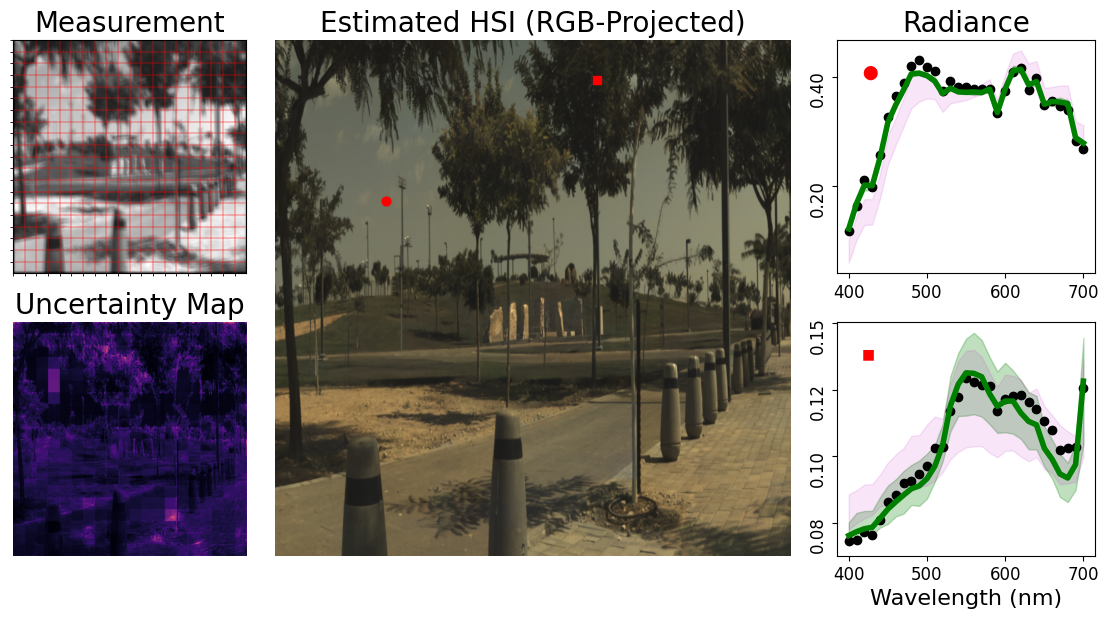
Figure 1: The RGB-projection and two representative spectra of a hyperspectral image reconstructed from the chromatic aberration encoded in a simulated grayscale measurement. Patches of the $1280\times 1280$ measurement are processed in parallel using guided diffusion, and the reconstructed HSI is sampled several times to assess uncertainty. Graphs show model outputs (green), ground truth (black), and ablated model outputs without guidance (magenta).

Snapshot hyperspectral cameras capture detailed spectral information about a scene at a single moment in time. They provide a richer representation than RGB images and are widely used for scientific detection and classification. Snapshot hyperspectral cameras have two coupled parts: an optical assembly that encodes a scene’s spatial and spectral information onto a photosensor, and a digital decoder that reconstructs the hyperspectral image (HSI) from the photosensor’s measurement. They employ three general strategies to make the reconstruction problem more tractable [14]: using complex, multi-stage optics; using a color filter array on the photosensor; and/or using a photosensor that has more pixels than the spatial size of the output HSI.

In this paper, we consider the reconstruction problem for a new, minimalist scenario that is less well-posed and previously unsolved. That is, we aim to reconstruct a hyperspectral image of size $H\times W\times 31$ when the photosensor pixels are unfiltered (grayscale), the number of measurement pixels ($H\times W$) is equal to the number of output pixels, and the optical assembly consists of only a single flat optic, like a diffractive optical element or a metalens. This scenario is interesting because being able to solve its reconstruction problem would enable a new class of snapshot hyperspectral cameras that are more compact and light-efficient. Even though it is severely ill-posed, there is hope that it is not impossible, because a flat optic can induce purposeful chromatic aberration (see Figure 2a) that helps encode spatial-spectral information into the available measurements.

We introduce a model that produces high-quality reconstructions for this inverse problem, and we show that no prior model is able to do so. Our model operates primarily in patches, so it can be trained using small HSIs and their simulated measurements, and then deployed on arbitrarily large ones. In addition, our model provides useful uncertainty maps, as depicted in Figure 1.

Our model succeeds by combining a patch diffusion process with cross-patch, physics-based guidance using the camera’s known optical response. We first train a conditional diffusion model that learns to map small grayscale measurement patches to a distribution of plausible hyperspectral patches. We then deploy this trained model to reconstruct a larger measurement by splitting it into patches, processing each patch in parallel with the diffusion model, and synchronizing the patch predictions using diffusion guidance. The guidance enforces that the collection of patch predictions, when stitched together, compose a full-field HSI that is optically consistent with the full-field measurement.

We test our method extensively in simulation. In addition to producing high-quality results for our minimalist scenario, we find it also performs well for a variety of previous snapshot hyperspectral imaging scenarios, such as CASSI [33], that are better conditioned. This suggests that models similar to ours could be developed for other computational sensing scenarios and modalities, such as depth and polarization. All code and data will be made publicly available. We summarize the contributions of this work as follows.

1. We conduct the first study of snapshot hyperspectral imaging using a filterless photosensor and a single lens, and we provide insight into lens designs for this task.

2. We show that previous models cannot perform well on this task, and we introduce a model that does.

3. We demonstrate the unique ability to process measurements of any size, reconstructing high-resolution HSIs across multiple datasets.

4. We show our model also achieves state-of-the-art performance when used in several other snapshot hyperspectral imaging scenarios that use different sensors and optics.

Figure 2: Forward model. (a) A hyperspectral scene is imaged through a diffractive lens, producing an optically-coded measurement on a filterless photosensor. (b) For a single HSI scene patch, (top) the point-spread function (PSF) induces a distinct blur and shift (bottom) at each wavelength and the measurement patch is the sum over wavelengths. Our patch diffusion model is trained to map a single measurement patch to its HSI scene patch; it must overcome the spatial mixing that occurs between patches.

2 Related Works

HSI Diffusion Models: Recent works have extended the application of diffusion models to HSIs. In aerial remote sensing where hyperspectral datasets are large, unconditioned diffusion models have been successfully trained from scratch to produce deep feature representations for classification [10, 43]. However, for natural scenes, HSI datasets are limited, so prior works have relied on using frozen, pre-trained RGB diffusion models to do plug-and-play HSI restoration [39, 51] and compressed sensing [38]. In our work, we train conditional hyperspectral diffusion models from scratch to better leverage spatial-spectral statistics. We overcome data scarcity by training on patches and reducing model size. To our knowledge, hyperspectral diffusion models have not been previously explored for predicting HSIs from compressed measurements.

Grayscale to Hyperspectral: Reconstructing HSIs from grayscale measurements has been previously achieved using multi-component optical systems such as CASSI [46, 33], which encodes spatial-spectral information with minimal ambiguity using relay lenses, a coded mask, a dispersive prism, and a photosensor with more pixels than those in the output HSI. Recent improvements to the digital decoder, such as incorporating channel-wise attention, have enabled steady improvements to reconstruction quality [47, 34, 33, 24, 23, 7, 9, 52]. Our approach differs in three ways. It replaces the CASSI’s multi-component optics with a flat diffractive element, and it reduces the size of the photosensor to have the same number of pixels as in the output HSI. Also, whereas CASSI decoders process the entire measurement at once, typically at a low spatial resolution, our model processes measurements in patches and so can be deployed on arbitrary measurement sizes.

RGB to Hyperspectral: A related direction explores reconstructing HSIs from measurements captured using a single lens but with a color filter array on the photosensor. The simplest examples use regular photographic lenses and common RGB Bayer filters, with digital decoders that perform spectral upsampling [1, 8, 2, 53]. Other systems use diffractive lenses [27, 54] or optimized color filter arrays [37, 35, 42, 32]. Our approach removes the requirement for a filter array on the photosensor and so increases light efficiency. While our model is designed for the more challenging problem of grayscale to hyperspectral, we find that it performs well for RGB measurements.

Deep-learned Colorization: Broadly, our work can also be seen as addressing a multi-channel generalization of the problem of inferring RGB colorization of grayscale images [55, 31, 25]. Our task similarly requires inverting a many-to-one mapping that can be ambiguous. Whereas previous RGB colorization approaches have used GANs to handle ambiguity [26], we instead use a denoising diffusion model.

3 Methods

A hyperspectral image (HSI) $\textbf{x}\in\mathcal{R}^{H\!\times\!W\!\times\!C}_{\geq 0}$ is defined to be a far-field scene’s undistorted spatial-spectral radiance after it is mapped to the photosensor plane by an ideal lens that is focused at infinity. This representation accounts for geometric magnification and spatial discretization to the sensor’s pixel size. We define the associated measurement $\mathbf{y}\in\mathcal{R}^{H\!\times\!W}_{\geq 0}$ that is induced by a diffractive optical element to be characterized by the element’s shift-invariant, wavelength-dependent point-spread function (PSF) $f(u,v,\lambda)$ via,

$$\mathbf{y}(u,v)\!=\!\mathcal{M}(\mathbf{x})\!=\!\sum_{\lambda}o(\lambda)\cdot f(u,v,\lambda)\!\underset{(u,v)}{*}\!\mathbf{x}(u,v,\lambda),$$ (1)

where $*$ denotes 2D convolution over the spatial dimensions, and $o(\lambda)$ corresponds to the spectral response of a panchromatic photosensor. A measurement is thus a linear optical encoding of a 3D hyperspectral cube to a 2D image, with the PSF inducing purposeful chromatic aberration that helps make the decoding problem more tractable.

In $\S$3.1, we discuss the lens and PSF designs that we use in our simulations. In $\S$3.2 and $\S$3.3, we review denoising diffusion and introduce our patch-based training scheme. Lastly, $\S$3.4 introduces our guided sampling algorithm, which synchronizes the patch predictions to produce full-field HSIs that are optically consistent with an input measurement.

3.1 Optical Encoding

For our optical encoders, we consider the set of spatial-spectral point-spread functions depicted in the middle row of Figure 3. These PSFs vary in the extent to which they spread spectral information across space, producing differently-blurred measurements. Importantly, we choose these PSFs because they can all be implemented by using a diffractive lens known as a metalens–a transparent glass sheet patterned with nanoscale cylinders of equal height and varying widths [30, 28]. The radius of each nanocylinder controls the local phase-delay, and each of the PSFs results from a different arrangement of radii. We computed these PSFs using the wave-optics simulator DFlat [19, 18, 6], which has been extensively validated in previous experiments. This provides confidence that these or comparable PSFs can be realized in future prototypes. Supplement $\S$A.1 provides additional details about our PSF design and simulation process.

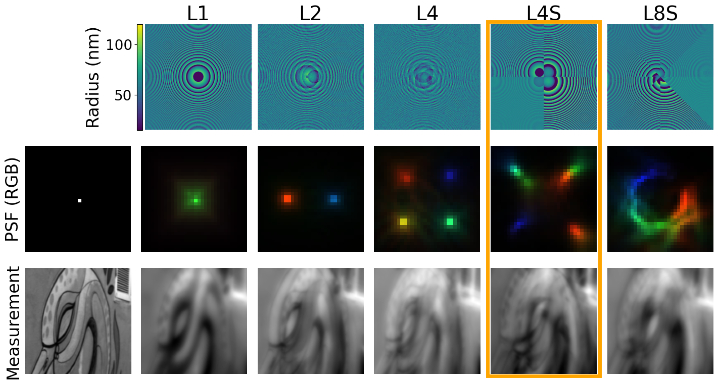
Figure 3: Spectral PSFs (middle row, projected to RGB) that are used in our experiments, each inducing a different type of chromatic smear. For context, we show the ideal achromatic PSF (left) and an example measurement for each PSF (bottom row). All of the PSFs can be fabricated using mature metalens technology, and the top row visualizes the nanocylinder radii pattern that creates each PSF.

3.2 Denoising Diffusion

Given a measurement $\mathbf{y}$, we use a conditional denoising diffusion probabilistic model to sample plausible hyperspectral images $\mathbf{x_{0}}$ from a distribution approximating the data distribution $q(\mathbf{x}|\mathbf{y})$. Following Ho et al. [21], we define a “forward process” $q(\mathbf{x}_{t}|\mathbf{x}_{t-1})\coloneqq\mathcal{N}(\mathbf{x}_{t};\sqrt{1-\beta_{t}}\mathbf{x}_{t-1},\beta_{t}\mathbb{I})$ that corrupts the HSI starting from $\mathbf{x}_{0}$ by adding Gaussian noise according to a variance schedule $\{\beta_{t}\}_{t=1...T}$. Intermediate, noisy HSIs $\mathbf{x}_{t}$ are given by

$$\mathbf{x}_{t}=\sqrt{\alpha_{t}}\mathbf{x}_{0}+\sqrt{1-\alpha_{t}}\mathbf{\epsilon},\mathbf{\epsilon}\sim\mathcal{N}(0,\mathbb{I}),$$ (2)

with $\alpha_{t}=\prod_{s=0}^{t}(1-\beta_{s})$. Assuming a sufficient variance schedule, the latent $\mathbf{x}_{T}$ converges to an isotropic Gaussian distribution for all $\mathbf{x}_{0}$, enabling the subsequent reverse process to be seeded by sampling $\mathbf{x}_{T}\sim\mathcal{N}(0,\mathbb{I})$.

The conditional “reverse process” $q(\mathbf{x}_{t-1}|\mathbf{x}_{t},\mathbf{y})$ is approximated by a neural network that models the Gaussian transition $p_{\theta}(\mathbf{x}_{t-1}|\mathbf{x}_{t},\mathbf{y})\coloneqq\mathcal{N}(\mathbf{x}_{t-1};\mu_{\theta}(\mathbf{x}_{t},t;\mathbf{y}),\beta_{t}\mathbb{I})$. Instead of predicting the posterior mean directly, $\mu_{\theta}$ is parameterized in terms of the noisy input image $\mathbf{x}_{t}$ and a network’s noise prediction $\epsilon_{\theta}(\mathbf{x}_{t},t;\mathbf{y})$. The noise prediction model $\theta$ is then trained by minimizing the error $L(\theta)\coloneqq\mathbb{E}_{x_{0},\mathbf{\epsilon},t}[\|\mathbf{\epsilon}-\mathbf{\epsilon}_{\theta}(\mathbf{x}_{t},t;\mathbf{y})\|^{2}]$, and a reverse diffusion step is computed via:

$$\mathbf{x}_{t-1} =\sqrt{\alpha_{t-1}}\hat{\mathbf{x}}_{0}(\mathbf{x}_{t})+\sqrt{1-\alpha_{t-1}-\sigma_{t}^{2}}\epsilon_{\theta}+w,$$ (3)

$$\hat{\mathbf{x}}_{0}(\mathbf{x}_{t}) =\frac{x_{t}-\sqrt{1-\alpha_{t}}\epsilon_{\theta}}{\sqrt{\alpha_{t}}}.$$

We adopt the DDIM sampling formalism [45], where $\sigma_{t}$ is a time-varying constant that controls the stochasticity of the reverse process and $w\sim\mathcal{N}(0,\sigma_{t})$. Although the forward process is defined for a fixed sequence of length $T$, DDIM samples using a shorter sub-sequence of $[1,...,T]$ to accelerate the generation.

3.3 Patch Training

Instead of denoising full-field HSIs directly, we apply diffusion to patches. For training data, we use captured full-field HSIs from various datasets [1, 2, 40, 11] and prerender the corresponding full-field measurements using Eq. 1. We then train our models using pairs of patches $(\mathbf{x}_{0}^{(i)},\mathbf{y}^{(i)})$ that are randomly cropped from the HSI-measurement pairs. We implement conditioning by concatenation as shown in Figure 4. Training a conditional patch-based model for this task seems challenging because, as shown in Figure 2b, the forward optical process spreads relevant signal outside of the conditional measurement patch. Nonetheless, we find that training leads to efficient and stable convergence.

We max-normalize each measurement patch $\mathbf{y}^{(i)}$ and each ground-truth HSI patch $\mathbf{x}_{0}^{(i)}$, and then we scale each of their values to the usual range $[-1,1]$. This means our model is trained to generate hyperspectral patches that are only accurate up to an unknown scale factor. In Supplement $\S$A.2, we discuss this choice further and show that learning to generate patches with exact scaling is inherently ill-defined. We correct for the unknown per-patch scales during guided sampling, discussed next.

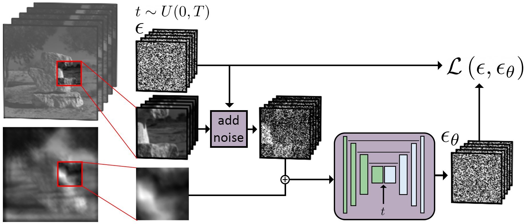
Figure 4: Diffusion training. Patches of fixed size are randomly cropped from ground truth HSIs and their corresponding measurements. A HSI patch is noised to timestep $t$, concatenated with the measurement patch, and passed to the noise prediction model.

3.4 Sampling with PSF Guidance

Applying the denoising formulation in Eq. 3 to patches yields hyperspectral patch predictions $\hat{\mathbf{x}}_{0}^{(i)}$ at intermediary time steps $t$. We can use this to guide the sampling of $\mathbf{x}_{t-1}^{(i)}$ from $\mathbf{x}_{t}^{(i)}$ by enforcing additional constraints on $\hat{\mathbf{x}}_{0}^{(i)}$. Previous works have used this strategy to solve inverse problems [12, 13]. In our work, we use it to enforce that all of the generated hyperspectral patches, when stitched together, produce a full-field HSI that is optically consistent with the full-field measurement according to Eq. 1. Pseudo-code is given in Algorithm 1. Throughout, we use superscript $p$ to denote a $p$-element collection of patches, e.g., $\mathbf{x}_{t}^{p}=\{\mathbf{x}_{t}^{(i)}\}_{i=1,...,p}$.

Algorithm 1 Guided Sampling

1:Initialize $\textbf{x}_{T}^{p}\sim\left\{\mathcal{N}(\textbf{0},\textbf{I})\right\}^{p}$

2:Initialize $\textbf{y}^{p}=\text{Patch}(\textbf{y},p)$

3:while $t>0$ do

4:  $\epsilon_{\theta}^{p}=\text{Model}(\mathbf{x}_{t}^{p},t;\mathbf{y}^{p})$ $\triangleright$ Computed in parallel

5:  for j = 0 to n do $\triangleright$ Guidance loop

6:   $c^{p}_{\text{lsq}}=\min_{c^{p}}\|\mathcal{M}(\text{Stitch}(c^{p}\cdot\hat{\mathbf{x}}^{p}_{0}(\mathbf{x}_{t}^{p})))-\mathbf{y}\|^{2}$

7:   $\mathcal{L}(\mathbf{x}_{t}^{p})=\|\mathcal{M}(\text{Stitch}(c^{p}_{lsq}\cdot\hat{\mathbf{x}}_{0}^{p}(\mathbf{x}_{t}^{p})))-\mathbf{y}\|^{2}$

8:   $\mathbf{x}_{t}^{p}=\mathbf{x}_{t}^{p}-\eta\nabla_{\mathbf{x}_{t}^{p}}\mathcal{L}(\mathbf{x}_{t}^{p})$

9:  end for

10:  $\mathbf{x}_{t-1}^{p}=\text{Denoise}(\mathbf{x}_{t}^{p},\epsilon_{\theta}^{p})$ $\triangleright$ From Eq. (7)

11:end while

12:$\mathbf{x}_{0}=\text{Stitch}(c_{lsq}^{p}\cdot\mathbf{x}_{0}^{p})$

During deployment, a full-field measurement $\mathbf{y}$ is split into a set of non-overlapping patches $\mathbf{y}^{p}$, which are concatenated with per-patch noise samples $\mathbf{x}_{T}^{p}$. The set of patches is processed in parallel to produce the intermediate denoised estimates $\hat{\mathbf{x}}_{0}^{p}$. We define a $\text{Stitch}()$ operator that combines these patch estimates into a full-field HSI, and then we input this estimated HSI to the measurement operation $\mathcal{M}()$ in Eq. 1. We use this rendered measurement in two ways. First, we compute optimal per-patch scale values $c^{p}_{\text{lsq}}\in\mathcal{R}^{p}$ by solving the least-squares problem,

$$c^{p}_{\text{lsq}}=\mathop{\mathrm{argmin}}_{c^{p}}\|\mathcal{M}(\text{Stitch}(c^{p}\cdot\hat{\mathbf{x}}^{p}_{0}(\mathbf{x}_{t}^{p})))-\mathbf{y}\|^{2},$$ (4)

which we do non-iteratively and efficiently for megapixel images by chunking and exploiting sparsity. Then, we rescale the denoised patch estimates via $c_{\text{lsq}}^{p}\cdot\hat{\mathbf{x}}_{0}^{p}$ before computing a guidance loss that measures consistency with the input full-field measurement:

$$\mathcal{L}(\mathbf{x}_{t}^{p},\mathbf{y})=\|\mathcal{M}(\text{Stitch}(c^{p}_{\text{lsq}}\cdot\hat{\mathbf{x}}_{0}^{p}(\mathbf{x}_{t}^{p})))-\mathbf{y}\|^{2}.$$ (5)

This loss guides the denoising updates to all patch predictions by modifying the standard denoising step in Eq. 3 via,

$$\tilde{\mathbf{x}}_{t}^{p} =\mathbf{x}_{t}^{p}-\eta\nabla_{\mathbf{x}_{t}^{p}}\mathcal{L}\left(\mathbf{x}_{t}^{p},\mathbf{y}\right)$$ (6)

$$\mathbf{x}_{t-1}^{p} =\sqrt{\alpha_{t-1}}\hat{\mathbf{x}}_{0}^{p}(\tilde{\mathbf{x}}_{t}^{p})+\sqrt{1-\alpha_{t-1}-\sigma_{t}^{2}}\epsilon_{\theta}^{p}+w^{p}.$$ (7)

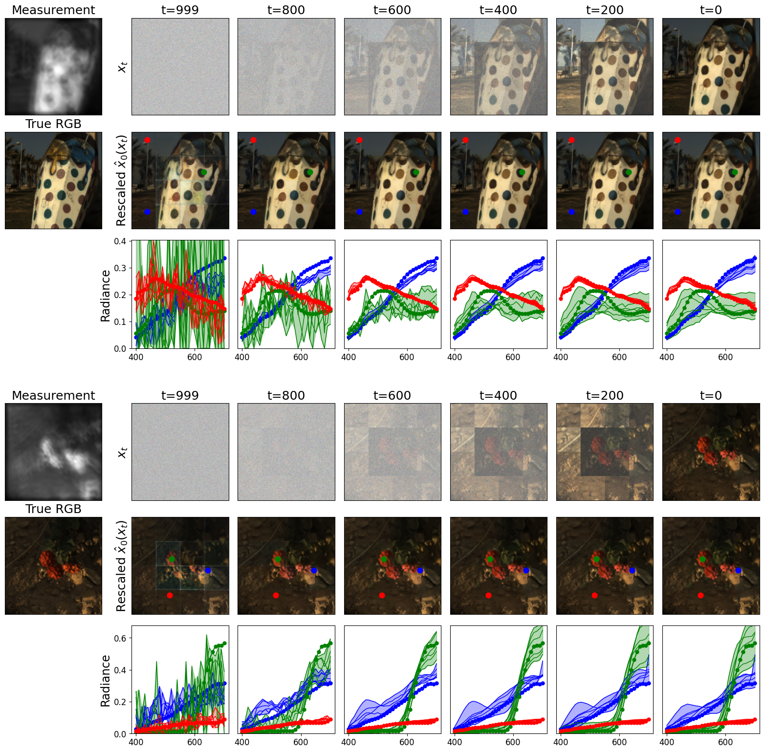
Figure 10: Time evolution of two reconstructed HSIs, sampled with guidance: The measurement is split into $16$ patches and the HSI prediction begins as random Gaussian noise. We display the intermediate patch predictions $\mathbf{x}_{t}^{p}$ and denoised patch estimates $\hat{\mathbf{x}}_{0}^{p}$ after they have been stitched together into the full-field HSIs $\mathbf{x}_{t}$ and $\hat{\mathbf{x}}_{0}$, respectively. The denoised estimates $\hat{\mathbf{x}}_{0}$ are displayed after patch rescaling using the coefficients $c_{\text{lsq}}^{p}$ from Eq. 4 in the main text. The line-plots display the predicted spectral radiance for the three demarcated pixels, with fill denoting the min-max predictions from a batch of samples (starting with different noise seeds). The spectral predictions become more accurate with each denoising timestep.

As is common, we repeat the gradient descent step in Eq. 6 multiple times before the denoising step in Eq. 7. We also find it useful to divide the gradient by its norm before scaling the step-size with $\eta$. An overview of the full sampling scheme is visualized in Figure 5, and we show the time evolution of HSI predictions in Supplement Figure 10.

We highlight that the diffusion model can generate different HSIs from the same measurement, by changing the initial noise seeds $\mathbf{x}_{T}^{p}$. We use this to compute a distribution of plausible inverse solutions by repeating the sampling algorithm multiple times. We then use the variance computed across repeated samples to capture spectral uncertainty. We define per-pixel spatial uncertainty maps from $N$ draws via,

$$\text{Uncertainty}=\sum_{\lambda}\mathrm{Var}\left(\{\mathbf{x}_{0}\}_{i=1}^{N}\right).$$ (8)

Figure 5: A full-field HSI is reconstructed by splitting the input full-field measurement into patches. Measurement patches are concatenated to hyperspectral patch predictions $\mathbf{x}_{T}^{(i)}$, which begin as Gaussian noise. Each hyperspectral patch is denoised to obtain an intermediate prediction $\hat{\mathbf{x}}_{0}^{(i)}$. Guidance comes from stitching these predictions into a full-field HSI, convolving and summing it with the spectral PSF, and comparing the result to the input full-field measurement. After guidance, the intermediate patch predictions are re-noised to the next timestep $t-1$, and the process repeats. We measure pixel-wise uncertainty by running the process several times with different random seeds.

4 Experiments

We evaluate our reconstruction algorithm in simulation considering three different datasets with spatial resolutions ranging from $256\times 256$ up to $1280\times 1536$. Based on our ablation studies reported in $\S$4.1, we use a patch size of 64 pixels for all experiments and render grayscale measurements using the L4S PSF, highlighted in Figure 3. For our denoising network, we adopt a UNet architecture with spatial attention, inspired by the RGB image synthesis models in [36, 21]. In contrast to their networks, we reduce the number of ResBlocks per layer by half while increasing the network depth. More details can be found in Supplement $\S$A.3.

In addition to our minimalist grayscale scenario, we also evaluate performance on other imaging scenarios, including using RGB measurements captured with and without our diffractive lens in $\S$4.1 and measurements captured with CASSI optics in $\S$4.3. Throughout, we sample using 50 DDIM steps and loop the guidance for 10 iterations. Uncertainty and mean spectra are derived by repeating the reconstruction 10 times with different noise seeds. We quantify accuracy with structural similarity (SSIM), peak signal-to-noise ratio (PSNR), and spectral angle (SAM) [50] computed over full hyperspectral images. For our diffusion model, we use the mean HSI averaged over repeated samples as a representative estimate. Additional details for each experiment are given in Supplement $\S$A.4 and we discuss the effect of measurement noise in Supplement $\S$A.5.

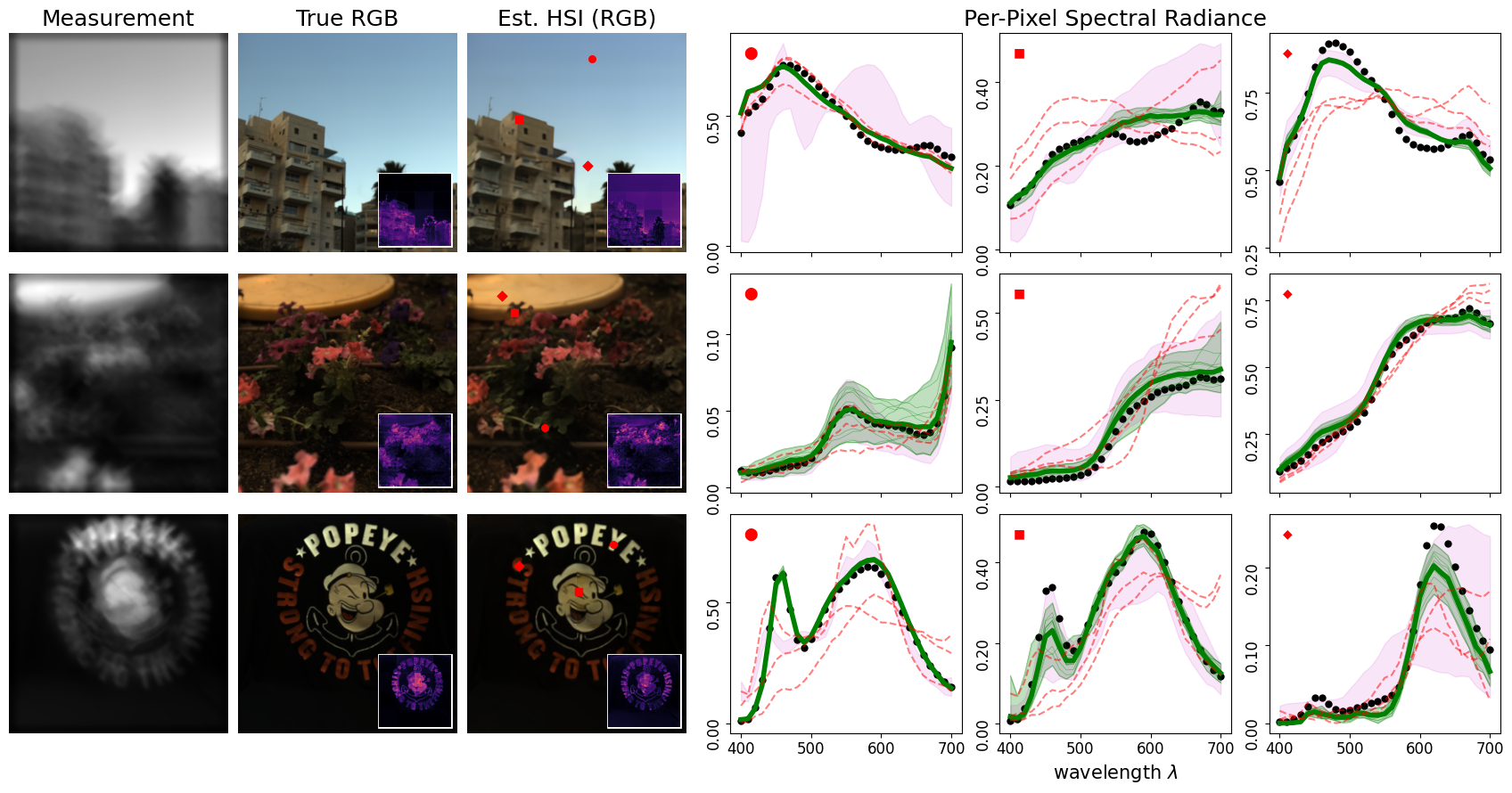
Figure 6: Grayscale-to-HSI reconstructions on the ARAD1K test set using the L4S PSF. True and estimated HSIs are projected to RGB, and insets show the reconstruction error (MSE, second column) and our computed uncertainty maps (third column). Graphs display three spectral profiles at pixel marked in red. Bold green is our model’s mean spectral estimate and black is ground truth. Green fill is the range of our model’s predictions over 10 samples (with guidance) and magenta fill is the same without guidance. Predictions from the three next-best comparison models are shown in dashed red.

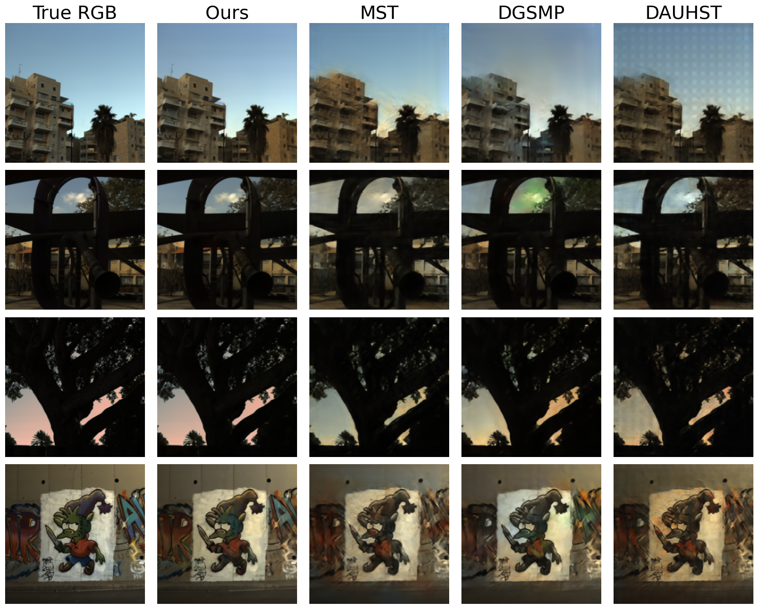
Figure 7: Comparison of our grayscale-to-HSI predictions vs other trained models, viewed in RGB colorspace.

Table 1: Reconstruction performance on the ARAD1K test set using grayscale (filterless) and RGB (Bayer) measurements, processed with our patch-diffusion model and several previous full-field hyperspectral models.

	Filterless + Optic			Bayer + Optic			Bayer
Model	SAM $\downarrow$	SSIM $\uparrow$	PSNR $\uparrow$	SAM $\downarrow$	SSIM $\uparrow$	PSNR $\uparrow$	SAM $\downarrow$	SSIM $\uparrow$	PSNR $\uparrow$
Ours	0.12	0.94	34.34	0.06	0.98	41.23	0.07	0.99	45.31
Ours (no guid.)	0.15	0.90	31.55	0.07	0.97	39.00	0.06	0.99	45.43
DGSMP [24]	0.16	0.88	30.04	0.10	0.95	35.99	0.07	0.99	38.47
MST [8]	0.17	0.87	29.80	0.08	0.97	38.08	0.06	0.99	44.56
DAUHST [9]	0.17	0.86	29.72	0.10	0.95	36.04	0.07	0.99	43.51
HDNet [23]	0.17	0.86	29.34	0.08	0.96	36.53	0.06	0.99	44.17
TSANet [33]	0.20	0.87	29.22	0.14	0.93	33.73	0.13	0.96	37.92
UNet	0.15	0.83	29.12	0.07	0.97	38.08	0.08	0.99	42.93

4.1 Evaluations on the ARAD1K Dataset

We first train and evaluate our model on measurements rendered using the ARAD1K dataset [2], which contains 900/50 train/test HSIs captured in both indoor and outdoor settings. To enable comparisons to previous models that process full-field measurements without patching, we spatially downsample all HSIs in this section to $256\times 256$ and render full-field measurements at that size.

Comparison to Previous Models: We compare our patch-based diffusion model to a variety of alternative hyperspectral models. This includes five previous networks [24, 8, 9, 23, 33] and a single-stage UNet, whose architecture is a copy of the one used in our diffusion backbone. These alternative models map full-field (fixed-resolution) measurements to full-field HSIs. We train all models from scratch on our rendered measurements, adhering to their original training procedures. We introduce as few architectural modifications as possible, such as replacing the forward and adjoint operators with our measurement function.

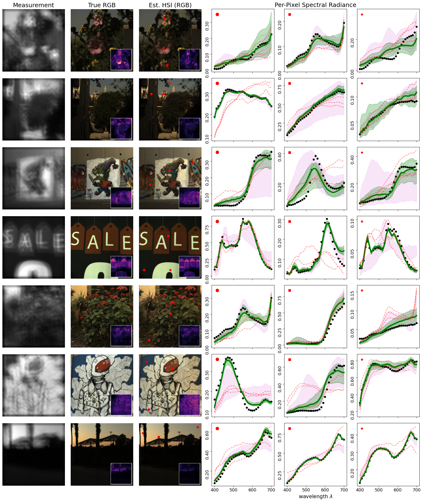
Figure 11: Additional HSI reconstructions on the ARAD1K test set: See caption in Figure 6 of the main text.

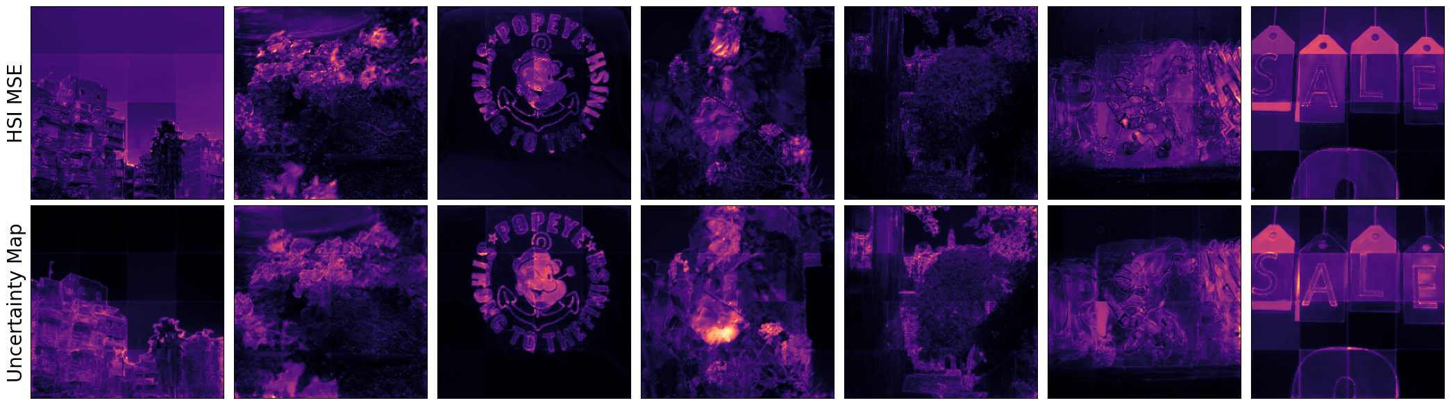
Figure 12: Enlarged MSE and uncertainty maps: These correspond to the insets from Figure 6 in the main text and selected insets from Supplement Figure 11. Images are rescaled with a gamma transformation $I^{\prime}=(I/\text{max}(I))^{0.5}$ to enhance visibility.

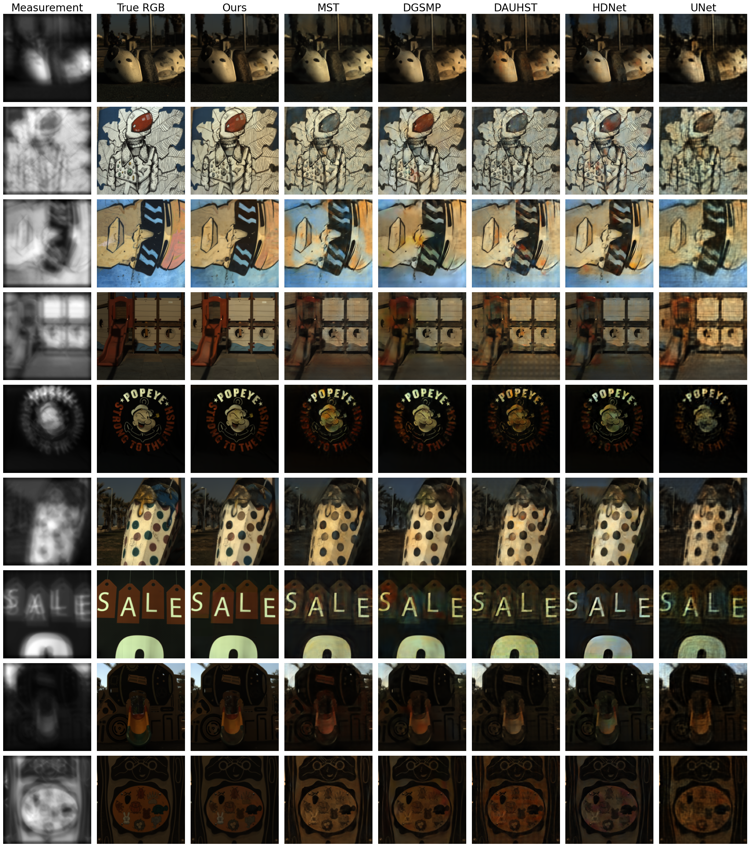
Figure 13: Additional comparisons of our HSI estimates (projected to RGB colorspace) vs other models: See Figure 7 of the main text for other examples.

The grayscale-to-hyperspectral reconstruction results are shown in the left-most column of Table 1 and in Figures 6–7. (See also Supplement Figures 11–13). Our model achieves an average PSNR of $34.34$, which is $4.3$ dB higher than the next best model. We also achieve a substantially higher SSIM than other models ($0.94$ vs. $0.88$), which reflects the large improvement in visual quality when viewing the HSIs projected to RGB space. These results show that our guided diffusion model is the only network capable of solving this problem successfully. It also suggests there is an advantage to concentrating neural capacity into local patches and tying them together with guidance, as opposed to spreading out the neural capacity across larger receptive fields.

Our model also provides uncertainty maps, computed via Eq. 8, that closely mirror the mean-squared error (MSE) between predicted and ground-truth HSIs. (See also Supplement Figure 12). This suggests the uncertainty could be useful for assessing pixel-wise reliability when the model is deployed in the wild. The quantification and use of uncertainty is discussed further in $\S$4.2–4.3.

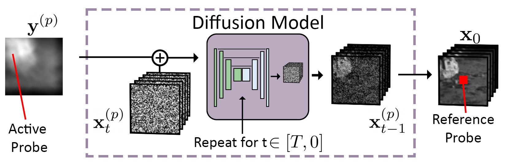
Figure 15: Visualization of the perturbation saliency calculation: We first generate a hyperspectral patch prediction $\mathbf{x}^{(p)}_{0}$, conditioned on the measurement patch $\mathbf{y}^{(p)}$. We then compute the saliency of a pixel $(i,j)$ in a measurement patch (the active probe) relative to a pixel $(r_{x},r_{y})$ in the output (reference probe) by setting that measurement pixel to zero, regenerating the hyperspectral patch prediction, and computing $\Delta\mathbf{x}^{(p)}_{0}(r_{x},r_{y})/\Delta\mathbf{y}^{(p)}(i,j)$. The same noise seed for $x_{T}^{(p)}$ is used with non-stochastic sampling via DDIM.

Model Ablations: Table 2 shows results on the ARAD1K dataset when using variations of our final model. We test a patch size of $32$ pixels instead of $64$, and we try using overlapping patches (Stride) with only the central portion of each patch’s prediction $\hat{\bf x}_{0}^{(i)}$ being used for stitching (Supplement Figure 15). We also test the effect of sampling without guidance (Guid.), which means omitting lines $5$–$9$ in Algorithm 1; and the effect of sampling without the patch-rescaling step, which means setting $c_{\text{lsq}}^{p}=1$ in line $6$. For the latter test, we use a separate diffusion model that was trained without patch normalization (discussed in $\S$3.3). We find that using overlapping patches has little effect when guidance is used but has a larger effect without guidance. This reaffirms that guidance is particularly important for pixels near patch boundaries and that it helps synchronize per-patch predictions. We also find that solving for the patch-rescale constants $c_{\text{lsq}}^{p}$ during sampling is important and results in a significantly higher PSNR. We attribute this performance gap to the ill-conditioning of our guidance loss when both the scale and shape of the spectral estimates are mismatched.

Comparison of Lens Designs: Table 3 evaluates the effect of the PSF design on the reconstruction quality, using the six PSFs displayed in Figure 3. Grayscale measurements are rendered with each, and separate diffusion models are trained for the same number of steps. We find that the reconstruction accuracy improves with greater spatial-spectral mixing but seems to do so asymptotically. From this, we suspect that choosing other PSFs that have a similar spatial extent would not substantially improve the results. To check whether simpler PSFs might result in HSI estimates that are spectrally inaccurate but perceptually plausible when projected to RGB, we project all generated HSI samples to RGB and compute the Fréchet inception distance (FID) [20] against the ground truth projected-RGB images. Interestingly, we find that FID also improves with PSF complexity, suggesting they produce better RGB-projections in addition to better HSIs.

Table 2: Ablation on Filterless + Optic reconstruction. We probe inference without patch rescaling (Resc.) and guidance (Guid.), and for overlapping patches (Stride). See text for more details.

Patch	Stride	Resc.	Guid.	SSIM $\uparrow$	PSNR $\uparrow$
64	32	✓	✓	0.94	34.48
64	-	✓	✓	0.94	34.34
64	32	✓	✗	0.92	32.37
64	-	✓	✗	0.90	31.55
32	-	✓	✓	0.93	33.27
32	-	✓	✗	0.87	29.27
64	-	✗	✓	0.92	31.77
64	-	✗	✗	0.86	27.54

Table 3: Lens Comparison. AIF refers to an all-in-focus lens with no chromatic aberration. All metrics are computed on full HSIs except for FID which is evaluated on RGB projections.

	AIF	L1	L2	L4	L4S	L8S
MSE $\downarrow$	0.15	0.13	0.09	0.04	0.04	0.04
SAM $\downarrow$	0.20	0.17	0.14	0.12	0.12	0.12
SSIM $\uparrow$	0.93	0.92	0.94	0.95	0.95	0.95
PSNR $\uparrow$	29.77	31.01	33.23	34.95	34.86	34.88
FID $\downarrow$	33.77	45.16	21.04	21.89	16.91	16.16

Interpretability: We probe the patch diffusion UNets that are trained for each PSF to examine what they have learned by computing perturbation saliency maps [44]. Given a pixel location $(r_{x},r_{y})$ in an output hyperspectral patch, we define the saliency of each input measurement pixel location $(i,j)$ to be $S(i,j\mid r_{x},r_{y})=\mathbb{E}_{p}\left[\sum_{\lambda}\lvert\partial\mathbf{x}_{0}^{p}(r_{x},r_{y},\lambda)/\partial\mathbf{y}^{p}(i,j)\rvert\right]$. For each diffusion UNet, we compute an approximation to this by setting measurement pixels to zero one-by-one, regenerating the final HSI prediction, and then recording the change in the spectra at the output pixel. No guidance is applied here, and saliency for each UNet is averaged over 20 randomly-drawn patches from its test set. The results are displayed in Figure 8. We find that the saliency maps closely match the structure of the PSF kernels that were used to generate the training data, even though these kernels were otherwise hidden from the model. This suggests that the UNets learn characteristics of the physical process that generates the data. Supplement Figures 15–16 show a visualization of this calculation and additional results where saliency reveals shift-invariance as would be expected from the convolution.

RGB Measurements: In the right two columns of Table 1, we report results from separate experiments for two alternative optical scenarios that have better conditioning. This includes using a Bayer-filtered photosensor with: (1) a diffractive lens that induces the L4S PSF (Bayer+optic) and (2) an ideal all-in-focus lens that induces no chromatic abberation (Bayer). We retrain our patch diffusion model in each case, with the only adjustment being an expansion of the measurement channel dimension from one to three. Again we find that our model provides substantially higher performance than all previous models. Interestingly, we also find that including an optic with a Bayer filter is generally worse than using perfectly focused measurements, and that guidance provides less of a benefit.

4.2 High-Resolution Challenge on ICVL Dataset

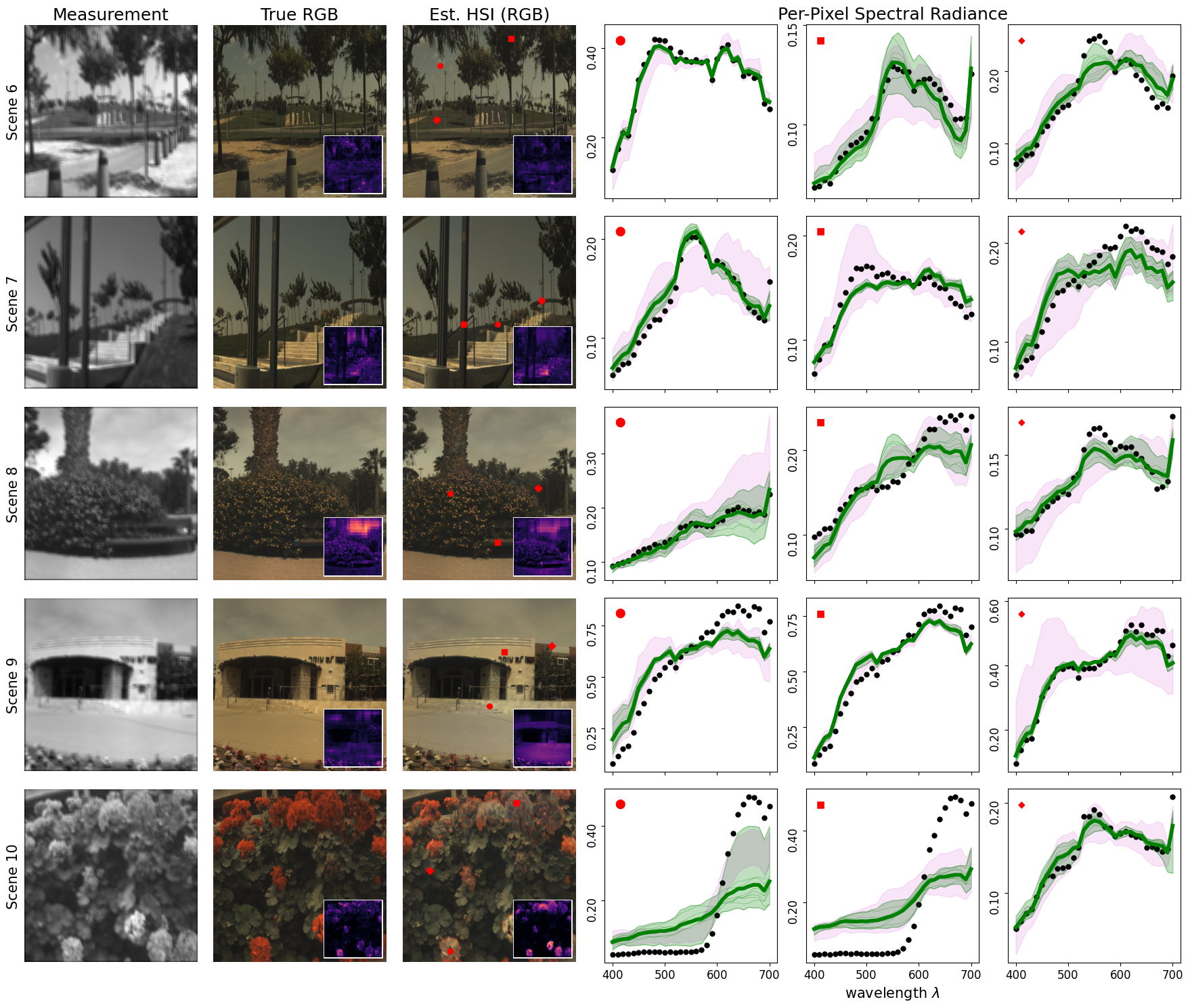
Figure 19: High-resolution 1280x1280 grayscale-to-HSI reconstructions on the ICVL dataset: Test Scenes 6-10. See caption in Supplement Figure 18 for more details.

A key advantage of our patch-based approach is that it enables the processing of arbitrarily large measurements. We demonstrate this by introducing a high-resolution reconstruction challenge. For this, we utilize the ICVL dataset [1], which contains $200$ real-world HSIs captured at a resolution of $1392\times 1300$ pixels. We reserve ten images for the testing set (resized to $1280\times 1280$) and allocate the remaining for training. To account for differences in sharpness between the ICVL and ARAD1K datasets (see Supplement Figure 17), we finetune our model from $\S$4.1 on the training subset, again using the L4S PSF for rendering grayscale measurements. After, we generate our reconstructions by denoising $400$ patches in parallel. Performance metrics for each test image is given in Table 4 and reconstructed HSIs are displayed in Figure 1 and Supplement Figures 18–19.

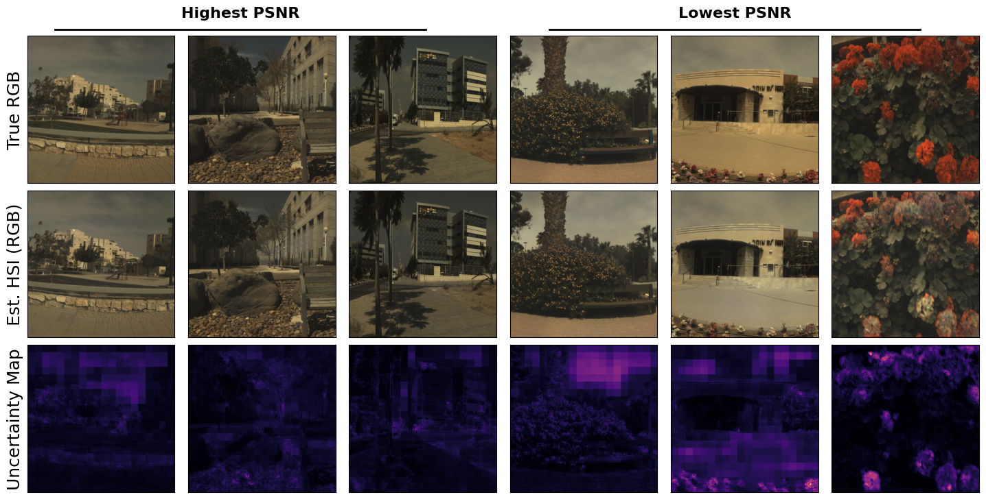
Figure 20: Visualization of uncertainty in ICVL HSI reconstructions: We display the HSI reconstructions (projected to RGB colorspace) with the 3 highest and 3 lowest average PSNR. Uncertainty maps are displayed with the same color scaling across all six images. We show qualitatively that the magnitude of predicted uncertainty accurately reflects the increased error in the estimates.

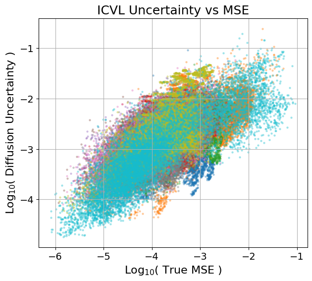
Figure 21: Scatter plot of uncertainty vs true MSE in ICVL HSI reconstructions: We randomly select $10$k pixels from each reconstructed HSI in the test set. Different colors correspond to different test images. We compute a Pearson correlation coefficient of 0.66 confirming that uncertainty is a strong predictor of error.

We find that our model performs well on all but two test scenes, producing HSIs that have minimal differences compared to the ground truth (as can be seen in the RGB projections). We also find that the generated uncertainty maps reasonably predict the failure cases. To further validate this, we compare the reconstruction MSE against the model’s uncertainty for randomly selected pixels and compute a Pearson’s correlation coefficient of $0.66$. This correlation is visualized in Supplemental Figures 20–22.

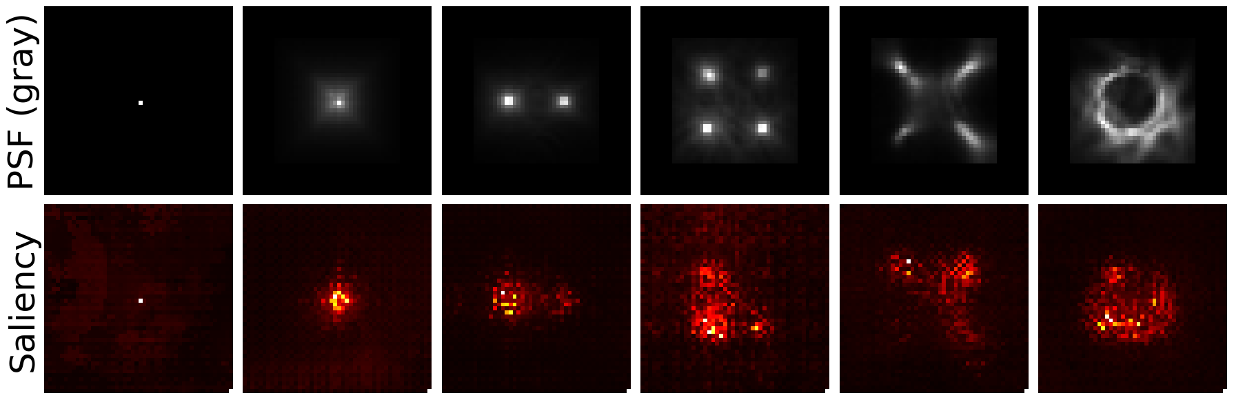
Figure 8: Perturbation Saliency Map: The saliency map highlights pixels in the input measurement patch that most influence the prediction at the center of the output HSI patch. See text for more details. Saliency should align with the PSF kernel used to generate the measurements.

4.3 Application to CASSI Measurements

We show that our patch reconstruction model also performs well when applied to an existing hyperspectral imaging system, specifically CASSI. In this scenario, the optics are more complex and the reconstruction task is better conditioned. To do this, we use the popular benchmark challenge from [33] and reconstruct HSIs of size $256\times 256\times 28$ from coded grayscale measurements of size $256\times 310$. Following prior works, the rendered grayscale measurements are pre-processed with a deshearing operation that extracts and stacks $256\times 256$ crops from the measurement with a stride along the smearing direction, as visualized in Supplement Figure 22. The condition to our diffusion model is then a 64-pixel patch extracted from the $256\times 256\times 28$ co-aligned measurement cube.

We train our diffusion model using HSIs from the CAVE [49] and ARAD1K datasets, and we test our model on the challenge’s $10$ HSIs extracted from the KAIST dataset [47]. A previous state-of-the-art model on this benchmark (outperforming prior algorithms by a large margin) is MST-L [7] with an average PSNR of $35.18$. Our model achieves an average PSNR of $35.46$. Moreover, by using our model’s generated uncertainty maps to exclude the $1\%$ and $5\%$ of pixels with the highest uncertainty values, our model’s average PSNR increases to $36.20$ and $37.31$. See the supplement for a complete table of results (Supplement Table 6) and for visualizations of the reconstructed HSIs (Supplement Figure 23).

Unlike all previous methods proposed for this benchmark, our model has the ability to also reconstruction larger CASSI measurements. Supplement Figure 24 shows $1280\times 1536$ pixel HSIs reconstructed from the KAIST dataset by denoising 480 patches in parallel.

Table 4: Grayscale-to-HSI reconstruction performance on the ICVL $1280\times 1280$ test set. Average metrics: SAM–0.08, SSIM–0.96; PSNR–33.83

Img	1	2	3	4	5	6	7	8	9	10
SAM	0.05	0.06	0.08	0.06	0.12	0.05	0.05	0.05	0.10	0.15
SSIM	0.96	0.97	0.96	0.97	0.96	0.96	0.97	0.96	0.94	0.93
PSNR	36.6	35.8	33.4	36.8	33.1	36.1	37.0	35.3	26.4	27.9

5 Limitations

One key limitation of our current model is its inability to capture long-range correlations across full-field measurements. The guidance step using the PSF enforces only local coherence. Consequently, the model may successfully reconstruct an object in one region of the image while failing to do so in another; this can be observed in the flowers at the bottom of Supplement Figure 19. Related to this, since our grayscale approach relies on chromatic aberration as a cue, the accuracy of individual patch predictions depends on the presence of spatial textures. Another notable limitation is our model’s compute time, as compared to previous single-stage models, when generating full-field HSIs using multiple guidance steps. For example, reconstructing the HSIs in $\S$4.1 on a single GPU takes approximately $59/30/1$ seconds when looping guidance $10/5/0$ times per denoising step.

6 Conclusion

This work introduces a new reconstruction model for snapshot hyperspectral imaging with a minimalist setup—a filterless photosensor and a single flat optic—that would make snapshot hyperspectral imaging more compact, efficient, and accessible. By developing the first diffusion-based model that is tailored to this under-determined scenario, we can produce high-quality HSIs at any spatial resolution using a simple optical configuration. We also demonstrate the versatility of our model by applying it to previous snapshot hyperspectral sensing scenarios that are better determined and achieving state-of-the-art results.

Appendix A Appendix

A.1 PSF Engineering and Metalens Design

Metalenses are designed by patterning fixed-height, transparent nanostructures across the surface of a glass substrate [28]. By carefully choosing the shape of the nanostructure at each location, a metalens can focus incident light of a single wavelength similar to a spherical lens [29, 30]. In contrast to refractive lenses, however, metalenses exhibit greater dispersion. This enables us to engineer distinct point-spread functions (PSFs) that have useful chromatic aberration. In this section, we discuss in detail the method used to generate our metalens designs. Code for all steps is provided in the project repository.

Following the approach of [30], we define a metalens $\mathbf{\Pi}$ as a collection of cylinders with varying radii $r$, arranged on a regular grid of points $\chi$, i.e. $\mathbf{\Pi}=\{r(x,y)\}_{\forall(x,y)\in\chi}$. We consider cylinders made of $\text{TiO}_{2}$, with a fixed height of $600$ nm and a grid spacing of $250$ nm. Given a particular configuration, the transformation that the metalens imparts to normally incident light of wavelength $\lambda$ can be computed by solving Maxwell’s equations for the transmitted field. We denote this mapping as $\Gamma$, which can be approximately evaluated point-by-point and defines a transmittance $t$ and phase delay $\phi$:

$$\Gamma\left(\mathbf{\Pi},x,y,\lambda\right)\approx\Gamma\left(r(x,y),\lambda\right)=t(x,y)e^{i\phi(x,y)}.$$ (9)

Pre-computed solutions for this mapping are displayed in Supplement Figure 9, evaluated for different wavelengths and nanocylinder radii using a finite-difference time-domain field solver [19].

In order to focus an incident plane wave of wavelength $\lambda$, the collection of nanocylinders on the metalens must be designed to induce a spatially-varying phase delay at that wavelength equal to:

$$\psi(x,y;\lambda)=\frac{2\pi}{\lambda}\left(c-\sqrt{d^{2}+(x-\delta u)^{2}+(y-\delta v)^{2}}\right),$$ (10)

where $c=\sqrt{d^{2}+\delta u^{2}+\delta v^{2}}$, $d$ is the axial distance to the photosensor, and $\delta u$ and $\delta v$ are the desired translational offsets of the focal spot.

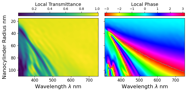
Figure 9: Nanocylinder Optical Response: The colormap displays the local transmittance (left) and phase delay (right) imparted to incident light of wavelength $\lambda$ that passes through a nanocylinder with radius $\in[15,110]$ nm. The phase imparted by a nanocylinder with a particular radius (row in the colormap) changes significantly with wavelength which causes chromatic aberration in the PSFs.

Notably, the wavelength dependence in $\Gamma$ (Eq. 9) generally does not match that in $\psi$ (Eq. 10). Consequently, a metalens configuration that realizes the focusing condition at one target wavelength will inherently fail to satisfy the focusing condition at all other wavelengths. We leverage this fact as a key principle to design PSFs with purposeful chromatic aberration. Specifically, we define an intermediary collection of metalenses that are each optimized to focus light under different conditions (incident wavelengths and focal positions), enumerated by the subscript $j$, via the following objective:

$$\mathbf{\Pi}_{j}=\min\limits_{r(x,y)}\left\|\Gamma\left(r(x,y),\lambda_{j}\right)-e^{i\psi(x,y;\lambda_{j},\delta u_{j},\delta v_{j})}\right\|^{2}.$$ (11)

We then spatially multiplex these intermediary metalenses using a set of orthogonal, binary selection masks $S_{i}$ [4, 16] to produce a final, composite metalens $\tilde{\mathbf{\Pi}}$:

$$\tilde{\mathbf{\Pi}}(x,y)=\sum_{j}S_{j}(x,y)\cdot\mathbf{\Pi}_{j}(x,y).$$ (12)

This process is repeated under different conditions to obtain the collection of composite metalenses evaluated in this work (Figure 3 in the main paper). We consider for our selection masks: (1) angular multiplexing, where each mask $S_{j}$ is set to $1$ for pixels within a particular angular range and $0$ elsewhere, like in metalenses “L4S” and “L8S”; and (2) spatial interleaving, where $S_{j}$ is a random binary mask, like in metalenses “L2” and “L4”.

Throughout, we label composite metalenses according to the number of intermediary metalenses that have been multiplexed. For example, “L2” combines two metalenses while “L4” combines four. We use the letter “S”, as in “L4S”, to denote a large shearing in the PSF, achieved by designing the intermediary lenses to focus off-axis with a large translational shift $\delta u$ and $\delta v$ in Eq. 10.

Finally, given a composite metalens $\tilde{\mathbf{\Pi}}$, we compute its intensity point-spread function $f$ by per-channel field propagation a distance $d$ using the Fresnel diffraction equation [15],

$$\begin{split}f(u,v,\lambda)&=\left\|\iint\Gamma\left(\tilde{\mathbf{\Pi}},x,y,\lambda\right)Q(u,v;x,y)\text{d}x\text{d}y\right\|^{2}\\ Q(u,v;x,y)&=\frac{e^{ikd}}{i\lambda d}\exp\left[\frac{ik}{2d}((x-u)^{2}+(y-v)^{2})\right].\end{split}$$ (13)

We set the distance $d$ (corresponding to the lens-to-sensor distance) to 1 cm and compute the PSF assuming a sensor pixel size of 5 $\mu m$. The spatial extent of the resulting PSFs are approximately fully confined to 64x64 pixels, $\approx$ 320 $\mu m$ in spread. The minimization in Eq. 11 and the propagation in Eq. 13 are computed using the open-source (PyTorch) package DFlat [19, 18]. This package also contains the pre-computed data for the optical mapping $\Gamma(r(x,y),\lambda)$ used in this work and displayed in Supplement Figure 9.

A.2 Patch Normalization during Training

As introduced in $\S$3.3 of the main paper, our diffusion model generates HSI patches, conditioned on measurement patches, that are accurate only up to a scale factor. We note that learning the exact scale for patches is generally challenging. In this section, we discuss the source of this difficulty and our decision to normalize patches during training.

We first consider the full-field HSI $\mathbf{x}$ and its corresponding full-field measurement $\mathbf{y}$, related by the operator $\mathbf{y}=\mathcal{M}(\mathbf{x})$ (Eq. 1 in the main paper). From the perspective of both data standardization and physical interpretation, we require a normalization applied to $\mathbf{x}$ and $\mathbf{y}$.

From a physical perspective, full-field HSIs must be normalized to ensure that HSIs differing only by a global scale factor are considered equivalent. This scale difference can be attributed to variations in the illumination source brightness, which should not influence downstream tasks like classification. Similarly, the measurements must be normalized to ensure that the prediction of a scene’s HSI does not change by altering the exposure time during capture. To address this, we normalize $\mathbf{x}$ and $\mathbf{y}$ by their max values as a pre-processing step. When extracting a pair of patches $\mathbf{x}_{0}^{(i)}$ and $\mathbf{y}^{(i)}$, we would then obtain the training pair:

$$\left(\frac{\mathbf{y}^{(i)}}{\text{max}(\mathbf{y})},\frac{\mathbf{x}^{(i)}_{0}}{\text{max}(\mathbf{x}_{0})}\right).$$ (14)

From the perspective of data standardization, we would require a similar normalization as well. Deep learning models are sensitive to the scale of input features and perform best when both the input and output are normalized to a standard range.

To see the problem with this formulation, however, we can equivalently consider this task in terms of learning from the training pair:

$$\left(\mathbf{y}^{(i)},\frac{{\text{max}(\mathbf{y})}}{\text{max}(\mathbf{x}_{0})}\mathbf{x}^{(i)}_{0}\right).$$ (15)

The target hyperspectral patch has its scale set by the factor $\text{max}(\mathbf{y})/\text{max}(\mathbf{x}_{0})$, which is indeterminable from looking at a measurement patch alone. In other words, the model input $\mathbf{y}^{(i)}$ matches to many target hyperspectral patches of different scales. For this reason, we instead max-normalize the patches directly, which results in the more well-posed training pair:

$$\left(\frac{\mathbf{y}^{(i)}}{\text{max}(\mathbf{y}^{(i)})},\frac{\mathbf{x}^{(i)}_{0}}{\text{max}(\mathbf{x}_{0}^{(i)})}\right).$$ (16)

This formulation satisfies data standardization and removes the scale ambiguity. As discussed in the main text, the optimal per-patch scales can later be identified by comparing the predicted measurement against the camera’s captured measurement.

A.3 Diffusion Model Parameters

We provide additional details for our diffusion model architecture and training schedule here. Our diffusion model utilizes a UNet backbone that is most similar in structure to the early RGB image synthesis models introduced by Ho et al. [21] (see also the PyTorch port by OpenAI in [36]). In contrast to their model, we use one ResBlock per stage instead of two/three. We also increase the UNet depth from four to five stages, meaning the network downsamples five times and then upsamples five times. We conducted several experiments early on and found that deeper models significantly outperformed wider models on this problem.

By introducing this change, we also substantially reduced the number of trainable parameters which helped to prevent over-fitting. In total, our UNet contains $75$M trainable parameters. For comparison, the ImageNet-64 diffusion model in [36] contains $270$M parameters in the UNet and Stable Diffusion 1 (2022) [41] contains approximately $890$M parameters.

In early explorations, we also extensively tested the use of attention applied along the channel dimension. Channel-wise attention is used in all prior hyperspectral neural networks evaluated in $\S$4.1 of the main paper. Broadly, it is also analogous to temporal attention found in most recent video diffusion models [22, 5, 48]. Interestingly, however, we found negligible improvement in performance when adding channel-wise attention to our diffusion UNets. We hypothesize that the spectral correlations in our task are simple enough to be captured fully by the 2D convolution blocks.

We provide a full summary of our model configuration in Supplement Table 5.

Parameter	Value
Beta Scheduler	Linear
Loss	L1 - Epsilon
Timesteps	$1000$
$K_{\text{min}}$-SNR [17]	$5.0$
Input Size	Patch size, $64\times 64$
Input Channels	$\lambda$-dim + $\mathbf{y}$-dim ($31+1$)
Output Channels	$\lambda$-dim ($31$)
Resblocks Per Stage	$1$
Time Embedding	$1024$
Time Embedding Scale+Shift	False
Layer Channels	[$64$, $128$, $256$, $512$, $512$]
Attention	All stages
Attention Head Dim	$32$
Group Norm Dim	$32$
Learning Rate	Cosine ($1\text{e}^{-4}$, $1\text{e}^{-6}$)
Batch Size	$64$
Skip-Connection Convolutions	False
Downsample Convolution	True
EMA	$0.9999$

Table 5: Summary of Model Configuration

A.4 Additional Experiment Details

Training: All models are trained from scratch for 72 hours using a single desktop NVIDIA RTX 3090 (32 GB) or equivalent GPU. Throughout, we apply random horizontal and vertical flip augmentations to the full-field HSIs before rendering measurements and extracting patches.

HSI Evaluation Metrics: We provide the formulas used for computing the evaluation metrics on HSIs. Following, we denote the full-field ground truth HSI as $\mathbf{x}(i,j,\lambda)$ and the reconstructed HSI as $\hat{\mathbf{x}}(i,j,\lambda)$ with shape $(H\times W\times C)$.

Although there are other formulations for PSNR when generalized to HSIs, we choose to follow the definition used in prior grayscale-to-hyperspectral works and compute the mean PSNR via,

$$\text{PSNR}=\frac{1}{C}\sum_{\lambda}10\text{ log}_{10}\left(\frac{\text{max}(\mathbf{x},\hat{\mathbf{x}})}{\frac{1}{HW}\sum_{i,j}(\mathbf{x}-\hat{\mathbf{x}})^{2}}\right).$$ (17)

We define the mean SAM via,

SAM $$=\frac{1}{HW}\sum_{i,j}\theta(i,j)$$ (18)

$$\theta(i,j) =\text{cos}^{-1}\left(\frac{\sum_{\lambda}\mathbf{x}\odot\hat{\mathbf{x}}}{\sqrt{(\sum_{\lambda}\mathbf{x}^{2})(\sum_{\lambda}\hat{\mathbf{x}}^{2}})}\right)$$ (19)

where $\odot$ denotes the Hadamard product. Lastly, we compute mean SSIM for HSIs by computing the standard single-channel 2D SSIM, denoted by operator $\mathcal{S}$, for each wavelength channel and then averaging via,

$$\text{SSIM}=\frac{1}{CHW}\sum_{i,j}\sum_{\lambda}\mathcal{S}(\mathbf{x(:,:,\lambda)},\hat{\mathbf{x}}(:,:,\lambda))$$ (20)

RGB Measurements: In $\S$4.1 of the main paper, we evaluate our reconstruction model when conditioned on three-channel RGB measurements. Each channel is rendered using Eq. 1, where the photosensor’s spectral response $o(\lambda)$ is set to the quantum efficiency of the R, G, and B channels in the Basler Ace 2 camera. Quantum efficiency estimates are taken from [3]. We note that our treatment does not take into account spatial demosaicing, which is necessary when using a Bayer filter mosaic. Consequently, we expect that our results represent an upper bound on performance, as it assumes no information loss when increasing the measurement channels.

ICVL Reconstructions: In $\S$4.2, we conduct experiments using the ICVL HSI dataset [1]. The original HSIs contain $519$ spectral bands, captured at wavelengths ranging from $400-1000$ nm. For our experiment, we keep only $31$ spectral bands between $400-700$ nm, linearly interpolated to 10 nm increments. This is done to match the ARAD1K dataset that is used in $\S$4.1. When finetuning our model, we initialize it with an existing checkpoint and train for an additional 24 hours using a fixed learning rate of $1\text{e}^{-6}$.

We also used the finetuned model to quantitatively analyze the relationship between per-pixel MSE and estimated uncertainty on the test set. To compute the Pearson correlation coefficient within memory constraints, we sampled a subset of $10$k pixels randomly from each reconstructed HSI. The relationship between MSE and uncertainty for these sampled pixels is visualized using color coding in Supplement Figure 22.

CASSI Reconstructions: In $\S$4.3, we train a diffusion model to process measurements captured using CASSI optics. The model is designed to reconstruct $28$ hyperspectral bands evenly spaced between $450$ nm and $650$ nm, following the HSI benchmark challenge proposed in [33]. Our combined training set consists of 32 HSIs from the CAVE dataset and 900 from the ARAD1K dataset, sampled without re-weighting. These HSIs are linearly interpolated to align with the model’s spectral channels.

A.5 Robustness to Measurement Noise

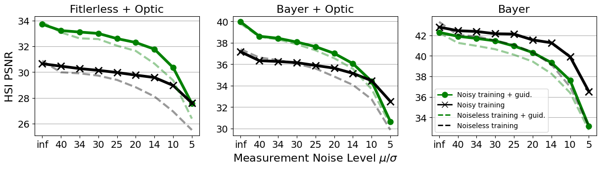
Figure 9: Reconstruction accuracy on the ARAD1K test set when measurements are corrupted with additive Gaussian noise: The amount of Gaussian noise added to each measurement (controlled by the variance $\sigma^{2}$) is tuned such that measurements are captured at fixed SNR$=\text{mean}({\mathbf{y}})/\sigma$. Noisy training means that the diffusion model was finetuned on noisy measurements and noiseless training means the model was only trained on noiseless measurements. Guid. refers to measurement-consistent guidance applied during sampling. See text for more details.

In this section, we show that our hyperspectral reconstruction algorithm performs well even when the captured measurements have significant noise. To demonstrate this, we simulate camera measurements $\mathbf{y}_{\text{noisy}}$ by adding Gaussian noise with variance $\sigma^{2}$ to the noiseless measurements via,

$$\mathbf{y}_{\text{noisy}}=\text{max}\left(\mathcal{M}(\mathbf{x})+\mathcal{N}(0,\sigma^{2}),\ 0\right),$$ (21)

where $\mathcal{M}$ is the noiseless measurement operator defined in Eq. 1 of the main paper. The max operation ensures that negative pixel values are clipped to zero.

To account for the measurement noise during reconstruction, we then modify our guidance loss function to a regularized least-squares loss via,

$$\mathcal{L}(\mathbf{x}_{t}^{p},\mathbf{y}_{\text{noisy}}) =\underset{\text{data fidelity}}{\underbrace{\frac{1}{\sigma^{2}}\|\hat{\mathbf{y}}-\mathbf{y}_{\text{noisy}}\|^{2}}}+\underset{\text{regularization}}{\underbrace{\zeta\text{TV}(\hat{\mathbf{y}})}}$$ (22)

$$\hat{\mathbf{y}} =\mathcal{M}\left(\text{Stitch}(c^{p}_{\text{lsq}}\cdot\hat{\mathbf{x}}_{0}^{p}(\mathbf{x}_{t}^{p}))\right)$$ (23)

The data fidelity term measures the squared error between the predicted observation $\hat{\mathbf{y}}$ and the noisy measurement $\mathbf{y}_{\text{noisy}}$, which is scaled by $1/\sigma^{2}$ to adapt to different noise levels. The TV-regularization term, $\text{TV}(\hat{\mathbf{y}})$, is applied to the predicted observation and discourages the generation of HSIs that reproduce the high-frequency noise in the measurement. This term is particularly effective because the measurements should be smooth due to convolution with the PSF, making the choice of the scaling factor $\zeta$ less sensitive. We set $\zeta$ to a fixed value of $1\text{e}^{2}$.

We investigate the model’s sensitivity to noise by reconstructing HSIs using two variations of our diffusion model: one trained on noiseless measurements and another finetuned on noisy measurements. The sampling process is guided by the regularized loss described above, with the number of guidance loops reduced from $10$ to $4$ (see Algorithm 1). For each test measurement, we adjust the variance $\sigma^{2}$ of the added Gaussian noise to achieve a fixed signal-to-noise ratio (SNR), defined as $\text{SNR}=\mu/\sigma$ where $\mu$ is the mean intensity of the measurement.

In the first variation, we use the models introduced in $\S$4.1 of the main paper, which were trained solely on noiseless measurements. In the second variation, we use models finetuned on noisy training pairs:

$$\left(\frac{\mathbf{y}^{(i)}_{\text{noisy}}}{\text{max}(\mathbf{y}^{(i)}_{\text{noisy}})},\frac{\mathbf{x}^{(i)}_{0}}{\text{max}(\mathbf{x}_{0}^{(i)})}\right).$$ (24)

During finetuning, noise levels are randomly sampled by selecting SNR values uniformly between $10$ and $\inf$ (no noise). We run this training for $24$ hours using a fixed learning rate of $1\text{e}^{-6}$.

We evaluate the reconstruction accuracy by computing the PSNR between the predicted and the ground truth HSIs, as defined in Eq. 17 (same as in the main paper). We test using measurements rendered from the three optical configurations (filterless and Bayer) discussed in $\S$4.1 and using different noise levels with an SNR between $5$ and $\inf$. The results from this study are shown in Figure 9. Each data point represents the average PSNR from 30 different test scenes, each resampled $5$ times. We also present results without guidance for comparison.

Our results show that reconstructions are reasonably robust to measurement noise for all three optical configurations. Moreover, training with noisy measurements improves the reconstruction performance when processing noisy measurements. This benefit is more pronounced when generating samples without guidance. In scenarios where the measurement contains purposeful chromatic aberration (Filterless+optic and Bayer+optic), guidance improves reconstruction results, but its benefits diminish as noise levels increase. When the measurement is highly corrupted (SNR $\approx$ 5), guidance during sampling becomes uninformative and can produce worse results. Notably, when processing all-in-focus RGB measurements (Bayer), guidance offers no improvement at any noise level, consistent to our finding in the main paper for noiseless measurements.

Lastly, we comment on our noise model choice. We evaluate a Gaussian noise model here because our guidance loss, of the form $\nabla_{\mathbf{x}_{t}}\|\mathcal{M}(\hat{\mathbf{x}}_{0}(\mathbf{x_{t}}))-\mathbf{y}_{\text{noisy}}\|^{2}_{2}$, is theoretically optimal for Gaussian noise. We expect to find similar results for other noise models, assuming that the guidance likelihood is appropriately adjusted. For example, with Poisson noise, one can adopt the guidance loss introduced by Chung et al. [12], of the form $\nabla_{\mathbf{x}_{t}}\|\mathcal{M}(\hat{\mathbf{x}}_{0}(\mathbf{x_{t}}))-\mathbf{y}_{\text{noisy}}\|^{2}_{\Lambda}$, where $\|\cdot\|_{\Lambda}$ denotes a particular weighted quadratic norm that is theoretically optimal for Poisson noise.

Figure 14: Visualization of strided patching and stitching: The principle is displayed here with an RGB image for clarity only. We use a patch size of 64x64 pixels and a 32x32 pixel stride. The strided patching is used to split a full-field measurement into overlapping patches. Each patch is passed as a condition to the diffusion model to generate a set of overlapping hyperspectral patch predictions. The stiching mask is used to combine the hyperspectral patch predictions, keeping only the pixels in the center (white) and discarding those in the overlapping region (black).

Figure 16: Additional perturbation saliency maps: We show saliency maps computed for the L8S PSF and diffusion model (similar to the rightmost column in Figure 8 in the main paper), but viewed here for other reference probe locations in the output hyperspectral patch. We find that the saliency aligns well with the PSF kernel and the structure shifts as the reference probe is moved. This property aligns with the shift-invariant rendering equation used to generate the measurement patches.

Figure 17: Comparison of textures in ICVL vs ARAD Patches: We randomly draw and display 20 hyperspectral patches from each dataset (not cherry-picked). We observe that the HSIs in the ICVL dataset are blurrier than in the ARAD1K which causes a domain-shift.

Figure 18: High-resolution 1280x1280 grayscale-to-HSI reconstructions on the ICVL dataset: Test Scenes 1-5. True and estimated HSIs are projected to RGB, and insets show the reconstruction error (MSE, second column) and our computed uncertainty maps (third column). Graphs display three spectral profiles at pixel marked in red. Bold green is our model’s mean spectral estimate and black is ground truth. Green fill is the range of our model’s predictions over 10 samples (with guidance) and magenta fill is the same without guidance.

Figure 22: CASSI measurement model: A scene HSI is modulated by the spatially-varying binary mask. Each wavelength channel is then sheared by a dispersive prism resulting in a wider grayscale measurement. The measurement is then “desheared” and stacked (see main text). The diffusion model is trained with patches randomly cropped from the ground truth HSI and the tiled measurement.

Figure 23: 256x256 grayscale-to-HSI reconstructions on the CASSI benchmark challenge: True and estimated HSIs are projected to RGB colorspace for visualization in the second and third row. To highlight the alignment of uncertainty and reconstruction errors, we overlay the diffusion uncertainty map on top of a grayscale projection of the estimated HSI in the fourth row. Graphs depict spectral radiance predictions for the pixels demarcated in red. Our mean prediction is given in bold green, ground truth in black, and the min-max estimate range with guidance (green) and without guidance (magenta) computed from repeated sampling.

Figure 24: High-resolution 1280x1536 grayscale-to-HSI reconstructions on the KAIST Dataset: We use our diffusion model trained on CASSI measurements to reconstruct HSIs that are substantially larger than in the benchmark challenge. Measurements are split into $480$ patches (denoted by the red grid) which are denoised in parallel. The first row of the ”Hyperspectral Slice” (right) displays our 2D radiance predictions for different spectral bands. The second row displays the ground truth. We find good agreement between the two.

Scene	TSA-Net [33]		DGSMP [24]		MST-S [7]		MST-L [7]		Ours		Ours-$99\%$		Ours-$95\%$
	PSNR	SSIM	PSNR	SSIM	PSNR	SSIM	PSNR	SSIM	PSNR	SSIM	PSNR	SSIM	PSNR	SSIM
1	32.03	0.89	33.26	0.92	34.71	0.93	35.40	0.94	35.60	0.95	36.25	0.96	37.53	0.97
2	31.00	0.86	32.09	0.90	34.45	0.93	35.87	0.94	33.88	0.95	34.51	0.95	35.56	0.96
3	32.25	0.92	33.06	0.93	35.32	0.94	36.51	0.95	37.79	0.95	37.92	0.95	38.17	0.96
4	39.19	0.95	40.54	0.96	41.50	0.97	42.27	0.97	43.15	0.98	44.13	0.99	44.84	0.99
5	29.39	0.88	28.86	0.88	31.90	0.93	32.77	0.95	34.94	0.97	35.64	0.97	37.06	0.98
6	31.44	0.91	33.08	0.94	33.85	0.94	34.80	0.95	34.80	0.96	36.11	0.97	38.17	0.97
7	30.32	0.88	30.74	0.89	32.69	0.91	33.66	0.93	32.29	0.93	32.93	0.93	33.90	0.94
8	29.35	0.89	31.55	0.92	31.69	0.93	32.67	0.95	33.53	0.95	34.98	0.96	37.42	0.97
9	30.01	0.89	31.66	0.91	34.67	0.94	35.39	0.95	36.83	0.95	37.05	0.96	36.88	0.96
10	29.59	0.87	31.44	0.93	31.82	0.93	32.50	0.94	31.80	0.94	32.25	0.95	33.64	0.97
avg	31.46	0.89	32.63	0.92	34.27	0.94	35.18	0.95	35.46	0.95	36.20	0.96	37.31	0.97

Table 6: CASSI reconstruction challenge full table: Comparison of our HSI reconstruction algorithm (trained on 64 pixel patches) vs previous state-of-the-art models (trained on full-size measurements) on ten test images extracted from the KAIST Dataset. Values for other methods are pulled from the recent work [8]. Ours-$X\%$ corresponds to the weighted metrics when keeping the X$\%$ of pixels with the lowest uncertainty, identified using our diffusion model uncertainty map.

References

- Arad and Ben-Shahar [2016] Boaz Arad and Ohad Ben-Shahar. Sparse recovery of hyperspectral signal from natural rgb images. In Computer Vision – ECCV 2016, pages 19–34. Springer International Publishing, 2016.
- Arad et al. [2020] Boaz Arad, Radu Timofte, Ohad Ben-Shahar, Yi-Tun Lin, Graham Finlayson, Shai Givati, et al. Ntire 2020 challenge on spectral reconstruction from an rgb image, 2020.
- Arad et al. [2022] Boaz Arad, Radu Timofte, Rony Yahel, Nimrod Morag, Amir Bernat, Yaqi Wu, Xun Wu, Zhihao Fan, Chenjie Xia, Feng Zhang, Shuai Liu, Yongqiang Li, Chaoyu Feng, Lei Lei, Mingwei Zhang, Kai Feng, Xun Zhang, Jiaxin Yao, Yongqiang Zhao, Suina Ma, Fan He, Yangyang Dong, Shufang Yu, Difa Qiu, Jinhui Liu, Mengzhao Bi, Beibei Song, WenFang Sun, Jiesi Zheng, Bowen Zhao, Yanpeng Cao, Jiangxin Yang, Yanlong Cao, Xiangyu Kong, Jingbo Yu, Yuanyang Xue, and Zheng Xie. Ntire 2022 spectral demosaicing challenge and data set. In 2022 IEEE/CVF Conference on Computer Vision and Pattern Recognition Workshops (CVPRW), pages 881–895, 2022.
- Arbabi et al. [2016] Ehsan Arbabi, Amir Arbabi, Seyedeh Mahsa Kamali, Yu Horie, and Andrei Faraon. Multiwavelength metasurfaces through spatial multiplexing. Scientific Reports, 6:32803, 2016.
- Blattmann et al. [2023] Andreas Blattmann, Robin Rombach, Huan Ling, Tim Dockhorn, Seung Wook Kim, Sanja Fidler, and Karsten Kreis. Align your latents: High-resolution video synthesis with latent diffusion models, 2023.
- Brookshire et al. [2024] Charles Brookshire, Yuxuan Liu, Yuanrui Chen, Wei Ting Chen, and Qi Guo. Metahdr: single shot high-dynamic range imaging and sensing using a multifunctional metasurface. Opt. Express, 32(15):26690–26707, 2024.
- Cai et al. [2022a] Yuanhao Cai, Jing Lin, Xiaowan Hu, Haoqian Wang, Xin Yuan, Yulun Zhang, Radu Timofte, and Luc Van Gool. Mask-guided spectral-wise transformer for efficient hyperspectral image reconstruction. In 2022 IEEE/CVF Conference on Computer Vision and Pattern Recognition (CVPR), pages 17481–17490, 2022a.
- Cai et al. [2022b] Yuanhao Cai, Jing Lin, Zudi Lin, Haoqian Wang, Yulun Zhang, Hanspeter Pfister, Radu Timofte, and Luc Van Gool. Mst++: Multi-stage spectral-wise transformer for efficient spectral reconstruction. In CVPRW, 2022b.
- Cai et al. [2022c] Yuanhao Cai, Jing Lin, Haoqian Wang, Xin Yuan, Henghui Ding, Yulun Zhang, Radu Timofte, and Luc Van Gool. Degradation-aware unfolding half-shuffle transformer for spectral compressive imaging, 2022c.
- Chen et al. [2023] Ning Chen, Jun Yue, Leyuan Fang, and Shaobo Xia. Spectraldiff: A generative framework for hyperspectral image classification with diffusion models. IEEE Transactions on Geoscience and Remote Sensing, 61:1–16, 2023.
- Choi et al. [2017] Inchang Choi, Daniel S. Jeon, Giljoo Nam, Diego Gutierrez, and Min H. Kim. High-quality hyperspectral reconstruction using a spectral prior. ACM Trans. Graph., 36(6), 2017.
- Chung et al. [2024a] Hyungjin Chung, Jeongsol Kim, Michael T. Mccann, Marc L. Klasky, and Jong Chul Ye. Diffusion posterior sampling for general noisy inverse problems, 2024a.
- Chung et al. [2024b] Hyungjin Chung, Byeongsu Sim, Dohoon Ryu, and Jong Chul Ye. Improving diffusion models for inverse problems using manifold constraints, 2024b.
- Ding et al. [2024] Kaiyang Ding, Ming Wang, Mengyuan Chen, Xiaohao Wang, Kai Ni, Qian Zhou, and Benfeng Bai. Snapshot spectral imaging: from spatial-spectral mapping to metasurface-based imaging. Nanophotonics, 13(8):1303–1330, 2024.
- Goodman [2005] J. W. Goodman. Introduction to Fourier Optics. Roberts & Co., Englewood, Colorado, 3rd edition, 2005.
- Guo et al. [2019] Qi Guo, Zhujun Shi, Yao-Wei Huang, Emma Alexander, Cheng-Wei Qiu, Federico Capasso, and Todd Zickler. Compact single-shot metalens depth sensors inspired by eyes of jumping spiders. Proceedings of the National Academy of Sciences, 116(46):22959–22965, 2019.
- Hang et al. [2024] Tiankai Hang, Shuyang Gu, Chen Li, Jianmin Bao, Dong Chen, Han Hu, Xin Geng, and Baining Guo. Efficient diffusion training via min-snr weighting strategy, 2024.
- Hazineh et al. [2023] Dean Hazineh, Soon Wei Daniel Lim, Qi Guo, Federico Capasso, and Todd Zickler. Polarization multi-image synthesis with birefringent metasurfaces. In 2023 IEEE International Conference on Computational Photography (ICCP), pages 1–12, 2023.
- Hazineh et al. [2022] Dean S. Hazineh, Soon Wei Daniel Lim, Zhujun Shi, Federico Capasso, Todd Zickler, and Qi Guo. D-flat: A differentiable flat-optics framework for end-to-end metasurface visual sensor design, 2022.
- Heusel et al. [2017] Martin Heusel, Hubert Ramsauer, Thomas Unterthiner, Bernhard Nessler, and Sepp Hochreiter. GANs trained by a two time-scale update rule converge to a local nash equilibrium. In Advances in Neural Information Processing Systems, pages 6626–6637. Curran Associates, Inc., 2017.
- Ho et al. [2020] Jonathan Ho, Ajay Jain, and Pieter Abbeel. Denoising diffusion probabilistic models, 2020.
- Ho et al. [2022] Jonathan Ho, Tim Salimans, Alexey Gritsenko, William Chan, Mohammad Norouzi, and David J. Fleet. Video diffusion models, 2022.
- Hu et al. [2022] Xiaowan Hu, Yuanhao Cai, Jing Lin, Haoqian Wang, Xin Yuan, Yulun Zhang, Radu Timofte, and Luc Van Gool. Hdnet: High-resolution dual-domain learning for spectral compressive imaging, 2022.
- Huang et al. [2021] Tao Huang, Weisheng Dong, Xin Yuan, Jinjian Wu, and Guangming Shi. Deep gaussian scale mixture prior for spectral compressive imaging, 2021.
- Iizuka et al. [2016] Satoshi Iizuka, Edgar Simo-Serra, and Hiroshi Ishikawa. Let there be color! joint end-to-end learning of global and local image priors for automatic image colorization with simultaneous classification. ACM Trans. Graph., 35(4), 2016.
- Isola et al. [2018] Phillip Isola, Jun-Yan Zhu, Tinghui Zhou, and Alexei A. Efros. Image-to-image translation with conditional adversarial networks, 2018.
- Jeon et al. [2019] Daniel S. Jeon, Seung-Hwan Baek, Shinyoung Yi, Qiang Fu, Xiong Dun, Wolfgang Heidrich, and Min H. Kim. Compact snapshot hyperspectral imaging with diffracted rotation. ACM Transactions on Graphics (Proc. SIGGRAPH 2019), 38(4):117:1–13, 2019.
- Khorasaninejad and Capasso [2017] Mohammadreza Khorasaninejad and Federico Capasso. Metalenses: Versatile multifunctional photonic components. Science, 358(6367):eaam8100, 2017.
- Khorasaninejad et al. [2016a] Mohammadreza Khorasaninejad, Wei Ting Chen, Robert C. Devlin, Jaewon Oh, Alexander Y. Zhu, and Federico Capasso. Metalenses at visible wavelengths: Diffraction-limited focusing and subwavelength resolution imaging. Science, 352(6290):1190–1194, 2016a.
- Khorasaninejad et al. [2016b] M. Khorasaninejad, A. Y. Zhu, C. Roques-Carmes, W. T. Chen, J. Oh, I. Mishra, R. C. Devlin, and F. Capasso. Polarization-insensitive metalenses at visible wavelengths. Nano Letters, 16(11):7229–7234, 2016b.
- Larsson et al. [2017] Gustav Larsson, Michael Maire, and Gregory Shakhnarovich. Learning representations for automatic colorization, 2017.
- Li et al. [2023] Ke Li, Dengxin Dai, and Luc Van Gool. Jointly learning band selection and filter array design for hyperspectral imaging. In 2023 IEEE/CVF Winter Conference on Applications of Computer Vision (WACV), pages 6373–6383, 2023.
- Meng et al. [2020] Ziyi Meng, Jiawei Ma, and Xin Yuan. End-to-end low cost compressive spectral imaging with spatial-spectral self-attention. In European Conference on Computer Vision, 2020.
- Miao et al. [2019] Xin Miao, Xin Yuan, Yunchen Pu, and Vassilis Athitsos. lambda-net: Reconstruct hyperspectral images from a snapshot measurement. In 2019 IEEE/CVF International Conference on Computer Vision (ICCV), pages 4058–4068, 2019.
- Monakhova et al. [2020] Kristina Monakhova, Kyrollos Yanny, Neerja Aggarwal, and Laura Waller. Spectral diffusercam: lensless snapshot hyperspectral imaging with a spectral filter array. Optica, 7(10):1298–1307, 2020.
- Nichol and Dhariwal [2021] Alex Nichol and Prafulla Dhariwal. Improved denoising diffusion probabilistic models, 2021.
- Nie et al. [2018] Shijie Nie, Lin Gu, Yinqiang Zheng, Antony Lam, Nobutaka Ono, and Imari Sato. Deeply learned filter response functions for hyperspectral reconstruction. In 2018 IEEE/CVF Conference on Computer Vision and Pattern Recognition, pages 4767–4776, 2018.
- Pan et al. [2024] Z. Pan, H. Zeng, J. Cao, K. Zhang, and Y. Chen. Diffsci: Zero-shot snapshot compressive imaging via iterative spectral diffusion model. In 2024 IEEE/CVF Conference on Computer Vision and Pattern Recognition (CVPR), pages 25297–25306, Los Alamitos, CA, USA, 2024. IEEE Computer Society.
- Pang et al. [2024] L. Pang, X. Rui, L. Cui, H. Wang, D. Meng, and X. Cao. Hir-diff: Unsupervised hyperspectral image restoration via improved diffusion models. In 2024 IEEE/CVF Conference on Computer Vision and Pattern Recognition (CVPR), pages 3005–3014, Los Alamitos, CA, USA, 2024. IEEE Computer Society.
- Park et al. [2007] Jong-Il Park, Moon-Hyun Lee, Michael D. Grossberg, and Shree K. Nayar. Multispectral imaging using multiplexed illumination. In ICCV, 2007.
- Rombach et al. [2022] Robin Rombach, Andreas Blattmann, Dominik Lorenz, Patrick Esser, and Bjorn Ommer. High-Resolution Image Synthesis with Latent Diffusion Models . In 2022 IEEE/CVF Conference on Computer Vision and Pattern Recognition (CVPR), pages 10674–10685, Los Alamitos, CA, USA, 2022. IEEE Computer Society.
- Salesin et al. [2022] Katherine Salesin, Dario Seyb, Sarah Friday, and Wojciech Jarosz. Diy hyperspectral imaging via polarization-induced spectral filters. In 2022 IEEE International Conference on Computational Photography (ICCP), pages 1–12, 2022.
- Sigger et al. [2024] N. Sigger, Q. T. Vien, S. V. Nguyen, et al. Unveiling the potential of diffusion model-based framework with transformer for hyperspectral image classification. Scientific Reports, 14:8438, 2024.
- Simonyan et al. [2013] Karen Simonyan, Andrea Vedaldi, and Andrew Zisserman. Deep inside convolutional networks: Visualising image classification models and saliency maps. CoRR, abs/1312.6034, 2013.
- Song et al. [2022] Jiaming Song, Chenlin Meng, and Stefano Ermon. Denoising diffusion implicit models, 2022.
- Wagadarikar et al. [2008] Ashwin Wagadarikar, Renu John, Rebecca Willett, and David Brady. Single disperser design for coded aperture snapshot spectral imaging. Appl. Opt., 47(10):B44–B51, 2008.
- Wang et al. [2019] Lizhi Wang, Chen Sun, Ying Fu, Min H. Kim, and Hua Huang. Hyperspectral image reconstruction using a deep spatial-spectral prior. In 2019 IEEE/CVF Conference on Computer Vision and Pattern Recognition (CVPR), pages 8024–8033, 2019.
- Wu et al. [2023] Jay Zhangjie Wu, Yixiao Ge, Xintao Wang, Stan Weixian Lei, Yuchao Gu, Yufei Shi, Wynne Hsu, Ying Shan, Xiaohu Qie, and Mike Zheng Shou. Tune-a-video: One-shot tuning of image diffusion models for text-to-video generation. In Proceedings of the IEEE/CVF International Conference on Computer Vision (ICCV), pages 7623–7633, 2023.
- Yasuma et al. [2010] Fumihito Yasuma, Tomoo Mitsunaga, Daisuke Iso, and Shree K. Nayar. Generalized assorted pixel camera: Postcapture control of resolution, dynamic range, and spectrum. IEEE Transactions on Image Processing, 19(9):2241–2253, 2010.
- Yuhas et al. [1992] Roberta H. Yuhas, Alexander F. H. Goetz, and Joe W. Boardman. Discrimination among semi-arid landscape endmembers using the spectral angle mapper (sam) algorithm. In Summaries of the Third Annual JPL Airborne Geoscience Workshop. JPL, 1992.
- Zeng et al. [2024] H. Zeng, J. Cao, K. Zhang, Y. Chen, H. Luong, and W. Philips. Unmixing diffusion for self-supervised hyperspectral image denoising. In 2024 IEEE/CVF Conference on Computer Vision and Pattern Recognition (CVPR), pages 27820–27830, Los Alamitos, CA, USA, 2024. IEEE Computer Society.
- Zhang et al. [2024] Jiancheng Zhang, Haijin Zeng, Jiezhang Cao, Yongyong Chen, Dengxiu Yu, and Yin-Ping Zhao. Dual prior unfolding for snapshot compressive imaging. In Proceedings of the IEEE/CVF Conference on Computer Vision and Pattern Recognition (CVPR), pages 25742–25752, 2024.
- Zhang et al. [2023a] Lei Zhang, Xiaoyan Luo, Sen Li, and Xiaofeng Shi. R2h-ccd: Hyperspectral imagery generation from rgb images based on conditional cascade diffusion probabilistic models. In IGARSS 2023 - 2023 IEEE International Geoscience and Remote Sensing Symposium, pages 7392–7395, 2023a.
- Zhang et al. [2023b] Qiangbo Zhang, Zeqing Yu, Xinyu Liu, Chang Wang, and Zhenrong Zheng. End-to-end joint optimization of metasurface and image processing for compact snapshot hyperspectral imaging. Optics Communications, 530:129154, 2023b.
- Zhang et al. [2016] Richard Zhang, Phillip Isola, and Alexei A Efros. Colorful image colorization. In ECCV, 2016.