Quasi-normal mode expansions of black hole perturbations: a hyperboloidal Keldysh’s approach

Abstract

We study asymptotic quasinormal mode expansions of linear fields propagating on a black hole background by adopting a Keldysh scheme for the spectral construction of the resonant expansions. This scheme requires to cast quasinormal modes in terms of a non-selfadjoint problem, something achieved by adopting a hyperboloidal scheme for black hole perturbations. The method provides a spectral version of Lax-Phillips resonant expansions, adapted to the hyperboloidal framework, and extends and generalises Ansorg & Macedo black hole quasinormal mode expansions beyond one-dimensional problems. We clarify the role of scalar product structures in the Keldysh construction [25] that prove non-necessary to construct the resonant expansion, in particular providing a unique quasinormal mode time-series at null infinity, but are required to define constant coefficients in the bulk resonant expansion by introducing a notion of ‘size’ (norm). By (numerical) comparison with the time-domain signal for test-bed initial data, we demonstrate the efficiency and accuracy of the Keldysh spectral approach. Indeed, we are able to recover Schwarzschild black hole tails, something that goes beyond the a priori limits of validity of the method and constitutes one of the main results. We also demonstrate the critical role of highly-damped quasinormal mode overtones to accurately account for the early time behaviour. As a by-product of the analysis, we present the Weyl law for the counting of quasinormal modes in black holes with different (flat, De Sitter, anti-De Sitter) asymptotics, as well as the $H^{p}$-Sobolev pseudospectra for the Pöschl-Teller potential.

L T

1 Introduction: quasi-normal (resonant) expansions and black hole ringdown

Resonant or quasi-normal mode (QNM) expansions of scattered fields play a key role in the description of open dissipative systems. They have been used systematically in the physics literature —(at least) since Gamow’s discussion of the $\alpha$ decay [24]— to describe the propagation of a linear field on a given background in terms of a superposition of damped oscillations, where the associated frequencies and time decay scales are characteristic properties of the background. From a mathematical perspective, they admit a sound descrip-tion in the Lax-Phillips and Vainberg scattering theory [40, 60]. In this mathematical setting, the resonant (or QNM) complex frequencies $\omega_{n}$ are characterised in terms of the poles of the meromorphic extension of the resolvent (essentially the Green function) of the wave equation. For concreteness, denoting formally the scattered field as $u(t,x)$ satisfying the following initial value problem of a linear wave equation (written in first-order Schrödinger form)

$$\displaystyle\left\{\begin{array}[]{l}\partial_{t}u=iLu\ ,\\ u(t=0,x)=u_{0}(x)\ ,\end{array}\right.$$ (3)

subject to ‘outgoing’ boundary conditions, the solution $u(t,x)$ can be expanded as an asymptotic series of damped sinusoids (cf. e.g. [57, 69, 19])

$$u(t,x)\sim\sum_{n}{\cal A}_{n}(x)e^{i\omega_{n}t}\ ,$$ (4)

where the complex frequencies $\omega_{n}$’s are the poles of the meromorphic extension of the resolvent of the infinitesimal time generator $L$, i.e. $R_{L}(\omega)=(L-\omega)^{-1}$, and the functions $a_{n}(x)$ are obtained by acting with such resolvent $R_{L}(\omega_{n})$ on the initial data $u_{0}(x)$, that is

$${\cal A}_{n}(x)=R_{L}(\omega_{n})(u_{0})\ .$$ (5)

The series (4) is an asymptotic one, in particular a non-convergent series in the generic case.

1.1 Normal modes in the conservative case

In contrast with this non-conservative (dissipative) situation above, the notion of normal modes in conservative systems provides an orthonormal basis where the solution $u(t,x)$ to the linear dynamics can be expanded. Specifically, given the initial value problem (3) with $L=H$ the selfadjoint time generator of the dynamics, acting in a Hilbert space ${\cal H}$ with scalar product $\langle\cdot,\cdot\rangle_{{}_{G}}$, its eigenfunctions $\hat{v}_{n}$ provide an orthonormal (Hilbert) basis such that the evolution $u(t,x)$ can be written as a convergent series

$$u(t,x)=\sum_{n=0}^{\infty}a_{n}\hat{v}_{n}(x)e^{i\omega_{n}t}\ ,$$ (6)

where

$$a_{n}=\langle\hat{v}_{n},u_{0}\rangle_{{}_{G}}\ ,\ \ \hbox{with}\ \ H\hat{v}_{n}=\omega_{n}\hat{v}_{n}\ ,$$ (7)

with $\omega_{n}$ real and $\langle\hat{v}_{n},\hat{v}_{m}\rangle_{{}_{G}}=\delta_{nm}$. Note that, in contrast with the prescription (4) and (5) for the dissipative case, the determination of the expansion (frequencies $\omega_{n}$’s and expansion coefficients $a_{n}$’s) in the conservative case reduces to a spectral problem. This spectral nature is at the basis of the powerful character of the expansion (6) and ultimately relies on the validity of the spectral theorem for selfadjoint (more generally, ‘normal’) operators.

1.2 Approaches to ‘completeness and orthogonality’ of QNMs in the dissipative case

In the non-selfadjoint (non-normal) case such a spectral theorem is absent and, therefore, no straightforward extension of the spectral approach underlying the normal mode expansion (6) is available. However, the formal comparison between the conservative and dissipative cases has prompted long-standing efforts in the physics literature to rewrite the asymptotic expansion (4) in a form more akin to the series (6), in particular in terms of a spectral problem with generalised eigenfunctions $v_{n}$ subject to QNM ‘outgoing boundary conditions’ that are, in general, non-normalisable. A considerable effort has been devoted to identify appropriate notions of ‘completeness’ and ‘orthogonality’ of the set of such generalised eigenfunctions $v_{n}$’s in this QNM dissipative setting, leading to different prescriptions in the spirit of Eq. (7) for determining the corresponding analogues of the (‘excitation’ [48]) coefficients $a_{n}$.

Specifically, in the gravitational setting and strongly motivated in recent times by the analysis in linear perturbation theory of the ringdown phase of binary black hole mergers, a large body of literature is available. As indicated above, various approaches involving different notions of completeness and orthogonality have been introduced in the literature, not always easily mutually comparable or just simply not compatible (see for instance [14] and [48] and references therein). Although rigorous notions of QNM completeness can be developed for certain potentials, as in the case of the Pöschl-Teller potential studied by Beyer [5], in constrast with the conservative (self-adjoint) case no appropriate general and sound notion of completeness for the expansion (10) is available for generic potentials, as plainly discussed in [61]. As commented above, the roots of this fact can be traced to the loss of spectral theorem in the non-selfadjoint (more precisely, ‘non-normal’) case.

1.3 The Keldysh approach to QNM resonant expansions

In the present work we do not dwell in the discussion above about completeness and orthogonality of the set of QNM functions $v_{n}$. We rather focus on the study of a systematic approach to render the resonant expansion (4) in terms of a proper spectral problem.

An underlying problem of many of the attempts mentioned above to cast resonant expansions in terms of a spectral problem is that the considered ‘generalised eigenfunctions’ are not normalisable, in particular they do not belong a well-controlled Banach space. This hinders the very definition of the QNM frequencies as ‘proper eigenvalues’ of the operator $L$. In contrast with this situation, in those cases in which the operator $L$ can be defined on a Hilbert space ${\cal H}$ (more generally on a Banach space) and QNM frequencies $\omega_{n}$’s can be characterised as proper eigenvalues of $L$, i.e. the $\omega_{n}$ values are (discrete) complex numbers in the point spectrum of $L$ —so the corresponding eigenfunctions are indeed normalisable— then a proper spectral approach can be devised for the resonant expansion (4). This is based in the so-called Keldysh expansion of the resolvent $R_{L}(\omega)$ in terms of the eigenvalue problem of the operator $L$ and its transpose operator $L^{t}$

$$Lv_{n}=\omega_{n}v_{n}\ \ ,\ \ L^{t}\alpha_{n}=\omega_{n}\alpha_{n}\ ,$$ (9)

where $v_{n}$ and $\alpha_{n}$ are usually referred to as right- and left-eigenfunctions of $L$ and, also, as modes and comodes, respectively (note that if $v_{n}$ belong to an linear (Banach) space ${\cal H}$, then $\alpha_{n}$ belong to a dual space ${\cal H}^{*}$). Crucially, they are normalisable (in the norm of the corresponding Banach space ${\cal H}$). As we will see below, the spectral problem (9) permits to expand the resolvent $R_{L}(\omega)$ in terms of $v_{n}$ and $w_{n}$, in such a way that (4) can be rewritten as

$$u(t,x)\sim\sum_{n}\big{(}a_{n}v_{n}(x)\big{)}e^{i\omega_{n}t}\ ,$$ (10)

where the QNM frequencies $\omega_{n}$’s are now proper eigenvalues of $L$, their corresponding QNM functions are the associated (normalisable) eigenfunctions $v_{n}$’s and the expansion coefficients $a_{n}$’s are obtained from the ‘action’ of the comode $w_{n}$ onto the initial data $u_{0}$ in a expression that parallels (see details later) the projection of $u_{0}$ onto $\hat{v}_{n}$ in expression (7) —note that in the selfadjoint (more generally ‘normal’) case ‘modes’ and ‘comodes’ do coincide.

An important point in the previous discussion is that different norms can be envisaged to measure de ‘size’ of modes and comodes, depending of the specific aspect we are studying. This freedom impacts the normalization of the QNMs $v_{n}$ and the value of the coefficients $a_{n}$. What remains invariant however is the product “$a_{n}v_{n}(x)$”, that provides a spectral reconstruction of the function $a_{n}(x)$ in the QNM resonant expansion (4), that is

$${\cal A}_{n}(x)=a_{n}v_{n}(x)\ ,$$ (11)

In essence, this expresion provides a ‘spectral prescription’ for the evaluation of ${\cal A}_{n}(x)$, as an alternative to the action of the resolvent in (5). However, it is a remarkable fact that this change of perspective translates into a powerful and efficient scheme to construct QNM expansions.

1.3.1 The present work: a hyperboloidal Keldysh approach to scattering and QNMs.

In this work we adopt the (spectral) Keldysh approach to QNM (asymptotic) expansions sketched above, revisiting and extending the discussion presented in [25].

A necessary condition to apply such a Keldysh expansion is that the time generator $L$ must be a properly defined non-selfadjoint operator acting in Hilbert (Banach) spaces. There are different manners of fulfilling this condition. A successful approach, used systematically in the calculation of QNMs in different physical and mathematical settings, is the so-called ‘complex scaling’ method (see e.g. [56, 46, 69]). Here he rather adopt a geometrical approach, akin to the discussion of spacetime causality and propagation properties in general relativity, namely the so-called hyperboloidal approach to scattering. In this scheme, spacetime is foliated by constant time spacelike ‘hyperboloidal hypersurfaces’ that asymptotically reach the spacetime regions attained by null rays, namely such hyperboloidal slices are transverse at regular cuts to future null infinity ${I}^{+}$ at large distances and to the event horizon ‘inner boundary’ in the case of black hole spacetimes. Very importantly, QNM eigenfunctions become then normalisable, in stark constrast with QNM functions defined on ‘Cauchy slices’.

In particular, this hyperboloidal procedure provides a geometrical implementation of the outgoing boundary conditions entering in the construction of QNMs, since the characteristics of the associated wave equations (along the light cones) become ‘outgoing’ at ${I}^{+}$ and the event horizon, so no causal degree of freedom can enter the integration domain from the boundary. At an analytical level, when combined with a (coordinate) compactification of the hyperboloidal slices, this approach recasts the boundary conditions into the (bulk) operator, that becomes ‘singular’ in the sense that the principal part appears multiplied by a function vanishing at the boundaries . In concrete terms, enforcing the outgoing boundaries conditions translates into enforcing appropriate (enhanced) regularity of the QNM functions.

In summary, adopting a hyperboloidal approach permits to characterise QNMs as (proper) eigenvalues of a well-defined non-selfadjoint operator, with (normalisable) eigenfunctions belonging to an appropriate Hilbert space. Such an approach to QNM in the BH setting has been pioneered by Warnick in [63] and Ansorg & Macedo in [3] and then further developed in subsequent works (cf. [52, 20, 21, 23, 33, 36, 37, 22, 62, 53] and references therein). In this non-selfadjoint setting, it is natural to consider the Keldysh expansion of the resolvent $R_{L}(\omega)$ of $L$. Exploiting this fact, Ref. [25] proposes precisely an approach to BH QNM resonant expansions built on the Keldysh expansion. In this work we revisit such Keldysh approach to QNM expansions focusing on the following points:

• Keldysh approach to QNM expansions: independence of the scalar product. We refine and extend the spectral approach in [25] for the construction of the version (10) of the asymptotic QNM resonant expansions (4), in particular stressing the fact —not sufficiently discussed in [25]— that such expansion is independent of the chosen scalar product, depending only on the transpose $L^{t}$ of $L$, rather than on its adjoint $L^{\dagger}$.

• Keldysh QNM expansions in BH scattering: an accurate and efficient prescription. We demonstrate numerically the remarkable acuracy of such Keldysh expansions in the BH setting, even with non-convergent asymptotic series and, most unexpectedly, when applying the Keldysh prescription beyond its domain of validity by including not only QNMs but also discrete approximations of the continuous ‘branch cut’ contribution.

Regarding its relation with previosus works, this Keldysh QNM expansion can be seen, on the one hand, as a generalization of the efficient spectral QNM expansions introduced by Ansorg & Macedo in [3]. Indeed, the scheme presented in [3] makes use of a discrete version of the Wronskian to construct the Green function (resolvent) that limits its application essentially to $1+1$ problems, whereas the Keldysh expansion permits a priori to extend the analysis to (odd) space dimensions. On the other hand, this Keldysh expansion connects with the QNM expansions discussed by Joykutty in [36, 37] in the BH scattering context, being precisely defined in terms of modes and comodes of the operator $L$. Following the suggestions in [36, 37], and emphasizing the absence of a fundamental role of a (definite-positive) scalar product in the Keldysh expansion —since the latter ultimately depends only ‘transpose’ (dual pairing) and not ‘adjoint’ (scalar product) notions— it is tantalizing to consider the relation of Keldysh QNM expansions with those QNM expansions proposed and discussed in [26].

The plan of the article is as follows. In section 2 we revisit the Keldysh expansion of the resolvent of a non-selfadjoint operator and apply it to the asymptotic resonant expansions in QNMs of a scattered field. In section 3 we give the elements of the evolution problem of a wave equation in the hyperboloidal scheme and identify the relevant non-selfadjoint infinitesimal time generator for the application of the Keldysh resonant expansion in this setting. Sections 4 and 5 contain the main results of this work. Specifically, in section 4 we implement numerically the hyperboloidal time-evolution by using a pseudo-spectral method and in section 5 we construct the Keldysh QNM resonant expansions demonstrating the remarkably performant spectral re-construction of the time-domain signal and insisting on the recovery of polynomial tails. We present in section 6 a short discussion of regularity aspects of QNMs and what role the scalar product plays the qualitative control of their excitation coefficients. Finally, in section 7 we present our conclusions.

2 Keldysh resonant expansions

In this section we revisit the Keldysh QNM expansion introduced in [25], but performing a crucial shift in the argument and construction: whereas in [25] a central role is endowed to the notion of scalar product in a given Hilbert space, here we will dwell on a more primitive version only involving the notion of a Banach space and its dual.

In Ref. [25] the use of Hilbert spaces and the associated adjoint operator $L^{\dagger}$ of a given operator $L$ were fully justified, since that article focuses on the different implications of the choice of a given scalar product in the discussion of BH QNM instability. However, in the specific context of QNM Keldysh expansions, such emphasis on the additional scalar product structure actually may eclipse the key underlying structures actually responsible of the expansion. In this section we provide such more general and, simultaneously, more basic account of QNM Keldysh expansions constructed on the basis of the transpose $L^{t}$ (and not the adjoint $L^{\dagger}$) operator. The connection with the scalar product can be made at a later stage.

2.1 Keldysh expansion of the resolvent

The construction is based on the notion of right- and left-eigenvectors, or modes and comodes, as defined in Eq. (9), that we rewrite as

$$\left(L-\omega_{n}\;\mathrm{I}\right)v_{n}=0\ \ ,\ \ \left(L^{t}-\omega_{n}\;\mathrm{I}\right)\alpha_{n}=0\ \ ,\ \ v_{n}\in{\cal H},\alpha\in{\cal H}^{*}\ .$$ (12)

In order to fully illustrate the generality of the procedure we consider a more general (in general non-linear) eigenvalue problem.

Following closely [6] (see also [45, 7, 47]), let us consider the application

$$\begin{array}[]{rccc}F:&\Omega&\longrightarrow&{\cal L}({\cal H},{\cal K})\\ &\omega&\mapsto&F(\omega)\end{array},$$ (15)

where $\Omega\in\mathbb{C}$ is a complex domain, ${\cal L}({\cal H},{\cal K})$ is the space of linear operators from the (complex) Banach space ${\cal H}$ into the Banach space ${\cal K}$. For all $\omega\in\Omega$, we assume the operator

$$F(\omega):{\cal H}\longrightarrow{\cal K}\ ,$$ (16)

to be Fredholm of index $0$. Defining the resolvent set $\rho(F)$ of $F$ as the subset of $\Omega$ where $F(\omega)$ is invertible, with inverse $(F(\omega))^{-1}$, we write the resolvent application $F^{-1}$ as

$$\begin{array}[]{rccc}F^{-1}:&\rho(F)\in\Omega&\longrightarrow&\cal{L}(\cal{K},\cal{H})\\ &\omega&\mapsto&(F(\omega))^{-1}\end{array}.$$ (19)

Under the conditions above, the spectrum $\sigma(F)$ of $F$, namely $\sigma(F)=\Omega\backslash\rho(F)$, is a discrete subset of $\Omega$ and the resolvent $F^{-1}$ is a meromorphic function.

Example 1. To fix and illustrate the points above, we note that in the case of the eigenvalue problem (12), the function $F$ is defined just by $F(\omega)=L-\omega\mathrm{I}$. Therefore the function $F^{-1}$ is the standard resolvent $R_{L}(\omega)$ of $L$, that is, $F^{-1}=\left(L-\omega\mathrm{I}\right)^{-1}=R_{L}(\omega)$. Under these assumptions, it follows that $R_{L}(\omega)$ is meromorphic in $\omega$.

We proceed now to discuss the Keldysh expansion. We consider the spaces ${\cal H}^{*}$ and ${\cal K}^{*}$, respectively the dual spaces of ${\cal H}$ and ${\cal K}$, and the transpose application $F^{t}(\omega)$ of $F(\omega)$

$$F(\omega)^{t}:{\cal K}^{*}\longrightarrow{\cal H}^{*}\ ,$$ (20)

defined by duality $\big{(}F(\omega)^{t}(\alpha)\big{)}(v):=\alpha\big{(}F(\omega)(v)\big{)}$ for all $v\in{\cal H}$ and all $\alpha\in{\cal K}^{*}$. Using the notation $\langle\cdot,\cdot\rangle$ for the dual pairing (cf. footnote 1) we rewrite these relations as $\langle F(\omega)^{t}(\alpha),v\rangle=\langle\alpha,F(\omega)(v)\rangle$. We take now a bounded subdomain $\Omega_{o}\subset\Omega$ and consider the ‘eigenvalue problems’ associated with $F(\omega)$ and $F(\omega)^{t}$, for $\omega\in\Omega_{o}$, namely the characterisation of their respective kernels. Under the assumptions above (see details in [7]) eigenvalues $\omega_{n}$ are isolated and we can write [45, 7, 47] the eigenvalue problems

$$F(\omega_{n})v_{n}=0\ \ ,\ \ F(\omega_{n})^{t}\alpha_{n}=0\ \ ,\ \ \hbox{with}\ v_{n}\in{\cal H},\ \alpha_{n}\in{\cal K}^{*}\ .$$ (22)

We assume in addition, for simplicity, that the $\omega_{n}$’s are non-degenerate (simple). Then, using the operator $F^{\prime}(\omega)=\frac{dF}{d\omega}\in{\cal L}({\cal H},{\cal K})$, obtained by deriving $F$ with respect to the spectral parameter $\omega$, we consider $\tilde{v}_{n}$ and $\tilde{\alpha}_{n}$ satisfying the following (relative) normalization

$$\langle\tilde{\alpha}_{n},F^{\prime}(\omega_{n})(\tilde{v}_{n})\rangle=1\ .$$ (23)

With these elements we can write the Keldysh expansion of the resolvent application $F^{-1}$, evaluated at $\omega\in\Omega_{o}\backslash\sigma(F)$, as follows [45, 7]

$$F^{-1}(\omega)=\sum_{\omega_{n}\in\Omega_{o}}\frac{\langle\tilde{\alpha}_{n},\cdot\rangle}{\omega-\omega_{n}}\tilde{v}_{n}+H(\omega)\ \ ,\ \ \hbox{with}\ \langle\tilde{\alpha}_{n},F^{\prime}(\omega_{n})(\tilde{v}_{n})\rangle=1\ .$$ (24)

where $H(\omega)\in{\cal L}({\cal H},{\cal K})$ is holomorphic in $\Omega_{o}$.

We can incorporate the normalization (23) in the expression of the resolvent as follows. Given $\alpha_{n}$ and $v_{n}$ satisfying the eigenvalue problem (22) but not subject to any particular normalization, then the modes $\tilde{v}_{n}$ and comodes $\tilde{\alpha}_{n}$ defined as

$$\tilde{v}_{n}=v_{n}\ \ ,\ \ \tilde{\alpha}_{n} = \frac{1}{\langle\alpha_{n},F^{\prime}(\omega_{n})(v_{n})\rangle}\alpha_{n}\ ,$$

satisfy

$$\langle\tilde{\alpha}_{n},F^{\prime}(\omega_{n})(\tilde{v}_{n})\rangle=\Big{\langle}\frac{1}{\langle\alpha_{n},F^{\prime}(\omega_{n})(v_{n})\rangle}\alpha_{n},F^{\prime}(\omega_{n})(v_{n})\Big{\rangle}=1\ ,$$ (25)

and we can write

$$F^{-1}(\omega)=\sum_{\omega_{n}\in\Omega_{o}}\frac{\langle\alpha_{n},\cdot\rangle}{\langle\alpha_{n},F^{\prime}(\omega_{n})(v_{n})\rangle}\frac{v_{n}}{\omega-\omega_{n}}+H(\omega)\ \ ,\ \ \omega\in\Omega_{o}\setminus\sigma(L)\ .$$ (26)

This expression of $F^{-1}(\omega)$ has the virtue of making explicit the weight $1/\langle\alpha_{n},F^{\prime}(\omega_{n})(v_{n})\rangle$ entering the structure of the resolvant. Note in particular that this expression (60) is invariant under arbitrary rescalings of $v_{n}\in{\cal H}$ and $\alpha_{n}\in{\cal H}^{*}$ so, in contrast with $\tilde{v}_{n}$ and $\tilde{\alpha}_{n}$ in expression (24) of $F^{-1}(\omega)$, $v_{n}$ and $\alpha_{n}$ are not subject to any given normalization.

Example 2. We apply the Keldysh construction of the resolvent to the case of the eigenvalue problem (12), with $F(\omega)=L-\omega\mathrm{I}$ as discussed in the Example 1. Taking into account that $F^{\prime}(\omega)=-\mathrm{I}$, we find as normalisation $\langle\tilde{\alpha}_{n},\tilde{v}_{n}\rangle=-1$. We can then write

$$R_{L}(\omega) = (L-\omega\mathrm{I})^{-1}=\sum_{\omega_{n}\in\Omega_{o}}\frac{\langle\tilde{\alpha}_{n},\cdot\rangle}{\omega-\omega_{n}}\tilde{v}_{n}+H(\omega)$$ (27)

$$= \sum_{\omega_{n}\in\Omega_{o}}\frac{\langle\alpha_{n},\cdot\rangle}{\langle\alpha_{n},F^{\prime}(\omega_{n})(v_{n})\rangle}\frac{v_{n}}{\omega-\omega_{n}}+H(\omega)$$

$$= \sum_{\omega_{n}\in\Omega_{o}}\frac{\langle\alpha_{n},\cdot\rangle}{\langle\alpha_{n},v_{n}\rangle}\frac{v_{n}}{\omega_{n}-\omega}+H(\omega)$$

$$= \sum_{\omega_{n}\in\Omega_{o}}\frac{\langle\alpha_{n},\cdot\rangle}{\omega_{n}-\omega}v_{n}+H(\omega)\ \ ,\ \ \omega\in\Omega_{o}\setminus\sigma(L)\ ,$$

where in the third line we have used $F^{\prime}(\omega)=-\mathrm{I}$ and in the fourth we have chosen $\langle\alpha_{n},v_{n}\rangle=1$. For concreteness, we will make use of the last expression of $R_{L}(\omega)$ in later sections, valid for modes $v_{n}$ and comodes $\alpha_{n}$ satisfying

$$Lv_{n}=\omega_{n}v_{n}\ \ ,\ \ L^{t}\alpha_{n}=\omega_{n}\alpha_{n}\ \ ,\ \ \hbox{with}\ \ \langle\alpha_{n},v_{n}\rangle=1\ .$$ (28)

The resolvent in the (bounded) $\Omega_{o}$ region is then expressed as a finite sum of poles (assuming that the $\omega_{n}$’s do not accumulate in $\Omega_{o}$) plus an analytical operator function $H(\omega)$. This finite sum will play a key role in the assessment of the infinite sum of QNM expansions (10) as an asymptotic expansion and not (in general) a convergent series, in contrast with the selfadjoint (normal) case in (6), as we see in the following subsection.

2.2 Keldysh asymptotic QNM resonant expansions

Let us apply the Keldysh construction of the resolvent to the wave problem, in Schrödinger form, defined in Eq. (3), that we rewrite as

$$\left\{\begin{array}[]{l}\partial_{\tau}u=iLu\ ,\\ u(\tau=0,x)=u_{0}(x)\ \ ,\ \ ||u_{0}||<0\end{array}\right.$$ (29)

denoting by $\tau$ the time parameter (see next section) and using an appropriate norm $||\cdot||$ in the Banach space of initial data. Following closely [25], we adopt a Laplace transform approach to solve (29). Considering $\mathrm{Re}(s)>0$

$$u(s;x):=\big{(}{\cal L}u\big{)}(s;x)=\int_{0}^{\infty}e^{-s\tau}u(\tau,x)d\tau\ ,$$ (30)

and applying it to (29) we obtain

$$s\;u(s;x)-u(\tau=0,x)=iLu(s;x)\ .$$ (31)

Dropping the explicit $s$-dependence and introducing $u(\tau\!=\!0,x)=u_{0}(x)$, from (29) we write

$$\big{(}L+is\big{)}u(s;x)=iu_{o}(x)\ ,$$ (32)

To solve this non-homogeneous equation we need the expression for the resolvent $\big{(}L+is\big{)}^{-1}=R_{L}(-is)$ of $L$, namely

$$u(s;x)=i(L+is)^{-1}u_{0}(x)=iR_{L}(-is)u_{0}\ .$$ (33)

This is the point in which the above-discussed Keldysh’s expansion of the resolvent enters into scene. Using the relation $s=i\omega$, we have $R_{L}(-is)=R_{L}(\omega)$, for $\omega\in\Omega_{o}\setminus\sigma(L)$, so

$$u(s;x)=iR_{L}(-is)u_{0}=iR_{L}(\omega)u_{0}\ \ ,\ \ \omega\in\Omega_{o}\setminus\sigma(L)\ ,$$ (34)

and employing expression (27) for the resolvent with modes and comodes in (28), we write

$$u(s;x) = i\sum_{\omega_{n}\in\Omega_{o}}\frac{\langle\alpha_{n},u_{0}\rangle}{\omega_{n}-\omega}v_{n}+iH(\omega)(u_{0})\ \ ,\ \ \omega\in\Omega_{o}\setminus\sigma(L)$$ (35)

$$= \sum_{s_{n}\in\Omega_{o}}\frac{\langle\alpha_{n},u_{0}\rangle}{s-s_{n}}v_{n}+i\tilde{H}(s)(u_{0})\ \ ,\ \ s\in i\Omega_{o}\setminus\sigma(L)\ ,$$

with $\tilde{H}(s)=H(-i\omega)$ an holomorphic function (and relative normalization $\langle\alpha_{n},v_{n}\rangle=1$).

The time-domain scattered field $u(\tau,x)$ is obtained with the inverse Laplace transform

$$u(\tau,x)=\frac{1}{2\pi i}\int_{c-i\infty}^{c+i\infty}e^{s\tau}u(s;x)ds\ ,$$ (36)

with $c\in\mathbb{R}^{+}$. Considering bounded domains $\Omega$ containing $[c-iR,c+iR]$ with $R\in\mathbb{R}^{+}$, we can write (under the hypothesis of convergence of this limit)

$$u(\tau,x) = \lim_{R\to\infty}\frac{1}{2\pi i}\int_{c-iR}^{c+iR}e^{s\tau}u(s;x)ds$$ (37)

$$= \lim_{R\to\infty}\frac{1}{2\pi i}\int_{c-iR}^{c+iR}e^{s\tau}\Big{(}\sum_{s_{n}\in\Omega_{o}}\frac{\langle\alpha_{n},u_{0}\rangle}{s-s_{n}}v_{n}+i\tilde{H}(s)(u_{0})\Big{)}ds\ .$$

Taking a contour $C$ in the $s\text{-}\mathbb{C}$ complex plane composed by the interval $[c-iR,c+iR]$ closed on the left half-plane by a semi-circle $S$ centered at $c+i0$ and of radius $R$, i.e. $C=[c-iR,c+iR]\cup S$, we denote by $\Omega_{R}$ the domain bounded by $C$ in $s\text{-}\mathbb{C}$. Under the hypotheses in section 2.1, the number of $s_{j}\in\Omega_{R}$ is finite and we can interchange the (finite) sum and the integral

$$u(\tau,x)=\lim_{R\to\infty}\Bigg{(}\sum_{s_{n}\in\Omega_{R}}\frac{1}{2\pi i}\oint_{C}e^{s\tau}\frac{\langle\alpha_{n},u_{0}\rangle}{s-s_{n}}v_{n}ds+\frac{1}{2\pi}\oint_{C}e^{s\tau}\tilde{H}(s)(u_{0})ds\Bigg{)}$$

$$-\lim_{R\to\infty}\Bigg{(}\sum_{s_{n}\in\Omega_{R}}\frac{1}{2\pi i}\int_{S}e^{s\tau}\frac{\langle\alpha_{n},u_{0}\rangle}{s-s_{n}}v_{n}ds+\frac{1}{2\pi}\int_{S}e^{s\tau}\tilde{H}(s)(u_{0})ds\Bigg{)}\ .$$ (38)

The integral of the analytic function $e^{s\tau}\tilde{H}(s)(u_{0})$ along the contour $C$ vanishes. For large enogh $R$, the first term of the integral along the (semi-)circle $S$ also vanishes. On the contrary, the second integral along the semi-circle $S$ does not in general vanish, depending on the particular function $\tilde{H}(s)$. Such last term then produces in general a term $C_{R}(\tau;u_{0})$. Then

$$u(\tau,x) = \lim_{R\to\infty}\Big{(}\sum_{s_{n}\in\Omega_{R}}e^{s_{n}\tau}\langle\alpha_{n},u_{0}\rangle v_{n}+C_{R}(\tau;u_{0})\Big{)}$$ (39)

$$= \lim_{R\to\infty}\Big{(}\sum_{\omega_{n}\in\Omega_{R}}e^{i\omega_{n}\tau}\langle\alpha_{n},u_{0}\rangle v_{n}+C_{R}(\tau;u_{0})\Big{)}\ ,$$

by applying the Cauchy theorem, where in the second line we have used the Fourier rather than the Laplace spectral parameter. The limit in expression (39) does not necessarily exist, in stark contrast with ‘normal’ (in particular selfadjoint) operators where the spectral theorem guarantees it. But, although such a resonant expansion for $u(\tau,x)$ cannot in general be written as a convergent series, as in the selfadjoint (normal) case in Eq. (6), a proper notion of asymptotic QNM resonant expansion does exist. We denote the latter formally as

$$u(\tau,x)\sim\sum_{n}e^{i\omega_{n}\tau}\langle\alpha_{n},u_{0}\rangle v_{n}\ \ ,\ \ \langle\alpha_{n},v_{n}\rangle=1\ .$$ (40)

The meaning of such asymptotic expression is the following. Given a (bounded) domain $\Omega$ in the complex plane, we can always write the exact solution to the evolution problem (29) as

$$u(\tau,x)=\sum_{\omega_{n}\in\Omega}e^{i\omega_{n}\tau}\langle\alpha_{n},u_{0}\rangle v_{n}(x)+E_{\Omega}(\tau;u_{0})(x)\ ,$$ (41)

where note that, under our assumptions, the number of terms in sum is finite. The key point is that the Keldysh expansion (39) permits to find a fine bound of the error $E_{\Omega}(\tau;u_{0})(x)$ made when approximating $u(\tau,x)$ by the finite sum. Specifically, choosing an appropriate norm and defining $a_{\Omega}=\max\{\mathrm{Im}(\omega),\omega\in\Omega\}$ them, from the structure of the integrand $e^{s\tau}\tilde{H}(s)(u_{0})$ in the last term in (2.2),we can estimate the norm of $E_{\Omega}(\tau;u_{0})(x)$ as

$$||E_{\Omega}(\tau;S)||\leq C(a_{\Omega},L)e^{-a_{\Omega}\tau}||u_{0}||\ ,$$ (42)

where $C(a_{\Omega},L)$ is a constant that depends on $a_{\Omega}$ and the evolution operator $L$ but, and this is a key point, not on the initial data $u_{0}$. In those cases where a finite number of QNMs are located in the region $\Omega$ (this will be the case in the black hole potentials we will consider later), we can count the QNMs in $\Omega$ with $n\in\{0,\ldots,N_{\mathrm{QNM}}\}$. We can then emphasize the number of QNMs employed in the approximation of the evolution field $u(\tau,x)$, rather than the considered region $\Omega$ in the complex plane containing those $N_{\mathrm{QNM}}+1$ modes, and rewrite

$$u(\tau,x) = \sum_{n=0}^{N_{\mathrm{QNM}}}e^{i\omega_{n}\tau}\langle\alpha_{n},u_{0}\rangle v_{n}(x)+E_{N_{\mathrm{QNM}}}(\tau;u_{0})$$

with $$||E_{N_{\mathrm{QNM}}}(\tau;u_{0})||\leq C(N_{\mathrm{QNM}},L)e^{-a_{N_{\mathrm{QNM}}}\tau}||u_{0}||\ .$$ (43)

In summary, we can write

$$u(\tau,x)\sim\sum_{n}e^{i\omega_{n}\tau}a_{n}v_{n}(x)\ \ \ ,\ \ \ \hbox{with}\ a_{n}=\langle\alpha_{n},u_{0}\rangle\ ,\ \ \langle\alpha_{n},v_{n}\rangle=1.$$ (44)

This provides the QNM resonant expansion of the propagating field in terms of its initial data. For completeness, we provide the expression of $a_{n}$ when we do not impose $\langle\tilde{w}_{n},\tilde{v}_{n}\rangle=1$ in (27). Repeating steps from (35) by inserting in (34) the expression of $R_{L}(-is)$ in the third line of (27), we finally get

$$a_{n}=\frac{\langle\alpha_{n},u_{0}\rangle}{\langle\alpha_{n},v_{n}\rangle}\ ,$$ (45)

so we can write

$$u(\tau,x)\sim\sum_{n}e^{i\omega_{n}\tau}\frac{\langle\alpha_{n},u_{0}\rangle}{\langle\alpha_{n},v_{n}\rangle}v_{n}(x)\ ,$$ (46)

where no normalisation is imposed on $\alpha_{n}$ and $v_{n}$ and, actually, the expression is explicitly invariant under (independent) rescalings of $\alpha_{n}$ and $v_{n}$.

Remarks. We recapitulate some important point in the construction:

• Generalization of the Ansorg & Macedo QNM expansions. The Keldysh QNM expansion (44) generalizes, to arbitrary dimension and in a general formalism valid for ‘arbitrary’ operators $L$, the one-dimensional QNM expansions introduced and (for the first time) implemented in the BH context by Ansorg & Macedo in  [3] (see also [2, 52]).

• No fundamental role of scalar product in QNM resonant expansions. The Keldysh expansion does not make use of scalar product structures, but only of the notion of duality and the associated transpose operator $L^{t}$, rather than the adjoint $L^{\dagger}$.

• No intrinsic ‘excitation coefficients’ $a_{n}$ in the Keldysh expansion. In the absence of a scalar product (or more generally a norm in ${\cal H}$), only the product “$a_{n}v(x)$” is well-defined. This can be easily seen in expressions (44) and (46). Indeed, if the norm of $v(x)$ is not fixed, we can rescale it by a factor $f\neq 0$. For concreteness, considering expression (44) for $u(\tau,x)$, from the constraint $\langle\alpha_{n},v_{n}\rangle=1$ we must rescale $\alpha_{n}$ by $1/f$, so $a_{n}$ is also rescaled by $1/f$, leaving the product “$a_{n}v(x)$” unchanged . The same conclusion follows, for arbitrary rescalings of $v_{n}$ and $\alpha_{n}$, from the scale invariant expression (46).

• Expansion coefficients $a_{n}$ and choice of scalar product. In contrast with the point above, scalar products (and more generally norms) provide an additional structure permitting to fix the norm of QNMs $v_{n}$’s and, consequently, the associated coefficients $a_{n}$. This is the setting adopted in [25] and we provide now the connection with this latter work.

  Given an operator $L:{\cal H}\to{\cal H}$, its transpose $L^{t}:{\cal H}^{*}\to{\cal H}^{*}$ is defined by its action $L^{t}(\alpha)$ on $\alpha\in{\cal H}^{*}$, with $\langle L^{t}\alpha,v\rangle=L^{t}(\alpha)(v)=\alpha(Lv)=\langle\alpha,Lv\rangle$, $\forall v\in{\cal H}$. If a scalar product $\langle\cdot,\cdot\rangle_{{}_{G}}$ is defined by $G:{\cal H}\times{\cal H}\to\mathbb{C}$, with $\langle v,w\rangle_{{}_{G}}=G(u,w)$, then the (formal) adjoint operator $L^{\dagger}$ is defined by $\langle v,Lw\rangle_{{}_{G}}=\langle L^{\dagger}v,w\rangle_{{}_{G}}$, $\forall v,w\in{\cal H}$. We can write then the associated systems of eigenvalue problems

  $$Lv_{n}=\omega v_{n}\ \ ,\ \ L^{t}\alpha_{n}=\omega\alpha_{n}\ \ ,\ \ v_{n}\in{\cal H},\alpha_{n}\in{\cal H}^{*}\ ,$$ (47)

  and

  $$Lv_{n}=\omega v_{n}\ \ ,\ \ L^{\dagger}w_{n}=\bar{\omega}w_{n}\ \ ,\ \ v_{n},w_{n}\in{\cal H}\ .$$ (48)

  In order to relate these eigenvalue systems, let us note that the scalar product $\langle\cdot,\cdot\rangle_{{}_{G}}$ defines an application $\Phi_{G}:{\cal H}\to{\cal H}^{*}$, with $\Phi_{G}(v)\in{\cal H}^{*}$, for $v\in{\cal H}$ defined by $\Phi_{G}(v)(w)=G(u,v)=\langle v,w\rangle_{{}_{G}}$, $\forall w\in{\cal H}$. Then the modes $\alpha_{n}\in{\cal H}^{*}$ and $w_{n}\in{\cal H}$, respectively in (47) and (48), are related as (cf. B for a justification in the finite rank (matrix) case)

  $$\alpha_{n}=\overline{\Phi_{G}(w_{n})}\ ,$$ (49)

  and it holds

  $$\langle w_{n},v\rangle_{{}_{G}}=\langle\alpha_{n},v\rangle,\ \ \forall v\in{\cal H}\ .$$ (50)

  Applying the latter expression for $v$ given by $v_{n}$ an $u_{0}$, we can write $a_{n}$ in (45) as

  $$a_{n}=\frac{\langle\alpha_{n},u_{0}\rangle}{\langle\alpha_{n},v_{n}\rangle}=\frac{\langle w_{n},u_{0}\rangle_{{}_{G}}}{\langle w_{n},v_{n}\rangle_{{}_{G}}}$$ (51)

  and we can write the asymptotic QNM resonant expansion (44) as (note $\tilde{v}_{n}(x)=v_{n}(x)$)

  $$u(\tau,x) \sim \sum_{n}e^{i\omega_{n}\tau}\frac{\langle w_{n},u_{0}\rangle_{{}_{G}}}{\langle w_{n},v_{n}\rangle_{{}_{G}}}v_{n}(x)$$ (52)

  $$= \sum_{n}e^{i\omega_{n}\tau}\frac{||w_{n}||_{{}_{G}}||v_{n}||_{{}_{G}}}{\langle w_{n},v_{n}\rangle_{{}_{G}}}\Big{\langle}\frac{w_{n}}{||w_{n}||_{{}_{G}}},u_{0}\Big{\rangle}_{{}_{G}}\frac{v_{n}(x)}{||v_{n}||_{{}_{G}}}$$

  $$= \sum_{n}e^{i\omega_{n}\tau}\kappa_{n}\langle\hat{w}_{n},u_{0}\rangle_{{}_{G}}\hat{v}_{n}(x)\ ,$$

  with $\hat{v}_{n}(x)$ and $\hat{w}_{n}(x)$ the modes and comodes normalised in the norm $||\cdot||_{{}_{G}}$ associated with the scalar product $\langle\cdot,\cdot\rangle_{{}_{G}}$, namely $||\hat{v}_{n}||_{{}_{G}}=||\hat{w}_{n}||_{{}_{G}}=1$, and

  $$\kappa_{n}=\frac{||w_{n}||_{{}_{G}}||v_{n}||_{{}_{G}}}{\langle w_{n},v_{n}\rangle_{{}_{G}}}\ ,$$ (53)

  the condition number of the eigenvalue $\omega_{n}$. The expression (52) recovers exactly the Eq. (153) in [25], generalising the expression for the “energy scalar product” $\langle\cdot,\cdot\rangle_{{}_{E}}$ to a general scalar product $\langle\cdot,\cdot\rangle_{{}_{G}}$.

  In summary, the scattered field admits a resonant expansion but the scattering problem by itself does not lead to a meaningful notion of (“excitation”) coefficients in the QNM expansion, either in the Lax-Phillips or the Keldysh version. For the latter, a measure of “large/small” is needed. This is provided by the notion of scalar product (or more generally a norm), in accordance with the strategy adapted in [25].

• General $F(\omega)=0$ problems: the “generalised eigenvalue problem” case. The standard eigenvalue problem (12) is not the only spectral problem $F(\omega)=0$ relevant in the context of QNM expansions. Another one particularly important in the BH setting that we will discuss later is given by the so-called generalised eigenvalue.

  We start by considering the evolution problem

  $$\left\{\begin{array}[]{l}B\partial_{\tau}u=iLu\ ,\\ u(\tau=0,x)=u_{0}(x)\ \ ,\ \ ||u_{0}||<0\end{array}\right.$$ (54)

  Taking the Laplace transform, the analogue of Eq. (55) is the non-homogeneous equation

  $$\big{(}L+isB\big{)}u(s;x)=iBu_{o}(x)\ .$$ (55)

  The homogeneous part, $\big{(}L+isB\big{)}u(s;x)=0$ and using $s=i\omega$, leads to the generalised eigenvalue problem

  $$Lu(\omega;x)=\omega Bu(\omega;x)=0\ \ \longleftrightarrow\big{(}L-\omega B\big{)}u(\omega;x)\ ,$$ (56)

  that we can rewrite as

  $$F(\omega)u(\omega;x)=0\ \ ,\ \ F(\omega)=L-\omega B\ .$$ (57)

  Following exactly the procedure (2.2) we can write

  $$u(\omega;x)=iF^{-1}(\omega)(Bu_{o})\ ,$$ (58)

  and then use Eq. (60) with

  $$F^{\prime}(\omega)=-B\ ,$$ (59)

  to write

  $$F^{-1}(\omega)=\sum_{\omega_{n}\in\Omega_{o}}\frac{\langle\alpha_{n},\cdot\rangle}{\langle\alpha_{n},Bv_{n}\rangle}\frac{v_{n}}{\omega_{n}-\omega}+H(\omega)\ \ ,\ \ \omega\in\Omega_{o}\setminus\sigma(L)\ .$$ (60)

  Finally, taking the inverse Laplace transform (36), we get to the alternative equivalent QNM resonant expansions

  $$u(\tau,x)\sim\sum_{n}e^{i\omega_{n}\tau}\frac{\langle\alpha_{n},Bu_{0}\rangle}{\langle\alpha_{n},Bv_{n}\rangle}v_{n}(x)$$ (61)

  where no particular normalisation is assumed for $\alpha_{n}(x)$ and $v_{n}(x)$ [in particular, one can adopt $\langle\alpha_{n},v_{n}\rangle=1$, in accordance with (40) and (44)] or, alternatively

  $$u(\tau,x)\sim\sum_{n}e^{i\omega_{n}\tau}\langle\alpha_{n},Bu_{0}\rangle v_{n}(x)\ \ ,\ \ \langle\alpha_{n},Bv_{n}\rangle=1\ ,$$ (62)

  by adapting the normalization to the structure of the generalised eigenvalue problem.

3 Hyperboloidal approach to scattering

In this section we present the form of the infinitesimal generator $L$ obtained when using a (compactified) hyperbolic approach to cast in Schrödinger form (3) the scattering problem

$$\left(\frac{\partial^{2}}{\partial\overline{t}^{2}}-\frac{\partial^{2}}{\partial\overline{x}^{2}}+\hat{V}\right)\phi=0\ ,$$ (63)

with initial data $\phi(\overline{t}=0,\overline{x})=\phi_{1}(\overline{x})$ and $\partial_{\overline{t}}\phi(\overline{t}=0,\overline{x})=\phi_{2}(\overline{x})$ in a Cauchy slice, subject to outgoing boundary conditions. For concreteness we focus on the $1+1$-dimensional problem, with $\overline{x}\in]-\infty,\infty[$ and then outgoing boundary conditions at $\overline{x}\to\pm\infty$. The ultimate goal is to illustrate the application of the Keldysh approach to the construction of QNM resonant expansions for scattered fields in such a hyperboloidal scattering problem.

3.1 The evolution problem: perturbations on spherically symmetric black holes

Having stated that generic setting, our specific focus in on the study such QNM resonant expansions in a class of scattering problems consisting in the propagation of a scalar, electromagnetic or gravitational field on a background given by (the domain of outer of communication of) a stationary spherically symmetric BH spacetime, by applying the Keldysh approach in the (compactified) hyperboloidal approach discussed in [66, 67, 63, 3, 52, 33, 49, 50, 68, 42]. We follow the treatment in these references, in particular adopting notation in [33], presenting only the essential elements are referring the reader to such references for further details. We start by considering the spherically symmetric line element

$$ds^{2}=-f(r)dt^{2}+f(r)^{-1}dr^{2}+r^{2}\Omega_{AB}dx^{A}dx^{B}\ ,$$ (64)

with $\Omega_{AB}$ the metric of the unit sphere and $r\in]r_{\mathrm{H}},\infty[$ with $r_{\mathrm{H}}$ the coordinate radius of the BH event horizon. We introduce the tortoise coordinate $r_{*}$, satisfying $dr/dr_{*}=f(r)$, with range $r_{*}\in]-\infty,\infty[$. Making use of the spherical symmetry scalar, electromagnetic or gravitational field perturbations can be written in terms of scalar master functions $\Phi$ that, once rescaled $\Phi=\phi/r$ and decomposed in spherical harmonics components $\phi_{\ell m}$, satisfy

$$\left(\frac{\partial^{2}}{\partial t^{2}}-\frac{\partial^{2}}{\partial r_{*}^{2}}+V_{\ell}\right)\phi_{\ell m}=0\ ,$$ (65)

where the expression $V_{\ell}$ depends on the BH background and on the nature of the field (its spin $s$). Boundary conditions for Eq. (65) in our scattering problem and in this Cauchy formulation are purely outgoing at (spatial) infinity ($r_{*}\to+\infty$) and purely ingoing at the horizon ($r_{*}\to-\infty$). For convenience, we introduce the dimensionless quantities

$$\bar{t}=\frac{t}{\lambda}\ \ ,\ \ \bar{x}=\frac{r_{*}}{\lambda}\ \ ,\ \ \hat{V}_{\ell} =\lambda^{2}V_{\ell},$$ (66)

in terms of a length scale $\lambda$ appropriately chosen in each problem, so Eq. (65) for pertubations on spherically symmetric BHs is cast in the form of the generic wave equation (63) above

$$\left(\frac{\partial^{2}}{\partial\overline{t}^{2}}-\frac{\partial^{2}}{\partial\overline{x}^{2}}+\hat{V}_{\ell}\right)\phi_{\ell m}=0\,.$$ (67)

3.2 Hyperboloidal scheme: outgoing boundary conditions and non-selfadjoint infinitesimal generator $L$

Massless perturbations (in odd space-dimensions) propagate along null characteristics reaching the wave zone modelled by null infinity ${I}^{+}$ at far distances and traversing the event horizon when propagating in a black hole spacetime. Considering first asymptotically flat spacetimes, outgoing boudary conditions are imposed at these respective outer and inner spacetime null boundaries. A natural manner of adapting the evolution problem to this propagation behaviour at the spacetime boundaries consists in choosing a spacetime foliation $\{\Sigma_{\tau}\}$ that is transverse to ${I}^{+}$ and the BH event horizon. From a geometric perspective, null cones are outgoing at the intersection between the slices $\Sigma_{\tau}$ at the spacetime boundaries, enforcing in a geometric manner the outgoing boundary conditions for physical fields . Hyperboloidal foliations, interpolating between the BH horizon and ${I}^{+}$, are therefore a natural setting in our scattering problem (cf. the excellent discussions in [50, 68, 42]).

On the other hand, the choice of such hyperboloidal foliations is particularly interesting in the setting of the Keldysh expansion of the resolvent discussed in section 2. Indeed the outgoing boundary conditions entail a loss of energy, namely a decrease of the norm of the scattered field (in an appropriately chosen norm) in the slice $\Sigma_{\tau}$ and, therefore, the evolution cannot be conservative (unitary) in such foliations. In order words, under the choice of hyperboloidal foliations to describe the time evolution, the enforcement of outgoing boundary conditions in the dynamical problem implies the non-selfadjoint nature of the infinitesimal time generator $L$, when Eq. (67) is written in the first-order form (3).

Hyperboloidal foliations therefore provide a natural setting to apply the Keldysh expansion in scattering problems, namely for the resolvent of the non-selfadjoint operator infinetimal time generator $L$. We sketch now the basic elements to cast the evolution problem in a hyperboloidal slicing (we follow closely the notation in [33], see [50, 68, 42] and references therein for a more extensive discussion). First we consider the coordinate change

$$\begin{cases}\bar{t}=\tau-h(x)\\ \bar{x}=g(x)\end{cases}\ .$$ (68)

The height function $h$ implements the hyperboloidal foliation, in such a way that $\tau=\mathrm{const.}$ slices are spacelike hypersurfaces penetrating the horizon and extending to future null infinity ${I}^{+}$. The function $g$ defines a compactification mapping of $\Sigma_{t}$ that brings (null) infinity at $\bar{x}\to+\infty$ and the horizon at $\bar{x}\to-\infty$ to a finite interval $]a,b[$, namely

$$g\colon]a,b[ \to]-\infty,+\infty[$$

$$x \mapsto\overline{x}=g(x)$$

Adding the points $a$ and $b$ implements the spatial compactification, allowing to incoporate null infinity ${I}^{+}$ and the BH horizon in the spatial domain $[a,b]$. Inserting the change of coordinates (68) into the wave equation (67), we get (we drop the indices $\ell$ and $m$)

$$-\partial^{2}_{\tau}\phi+L_{1}\phi+L_{2}\partial_{\tau}\phi=0\ ,$$ (69)

where the expression of the operators $L_{1}$ and $L_{2}$ are given by

$$L_{1} = \frac{1}{w(x)}\left(\partial_{x}(p(x)\partial_{x})-q(x)\right)$$

$$L_{2} = \frac{1}{w(x)}\left(2\gamma(x)\partial_{x}+\partial_{x}\gamma(x)\right)=\frac{1}{w(x)}\left(\gamma(x)\partial_{x}+\partial_{x}(\gamma(x)\cdot)\right)$$ (70)

with

$$p(x)=\frac{1}{|g^{\prime}|},\quad q(x)=\lambda^{2}|g^{\prime}(x)|V_{\ell},\quad w(x)=\frac{h^{\prime 2}-g^{\prime 2}}{|g^{\prime}|},\quad\gamma(x)=\frac{h^{\prime}}{|g^{\prime}|}\ .$$ (71)

Here $L_{1}$ is a singular Sturm-Liouville operator, with $p(x)$ vanishing at the boundary of the interval, i.e. $p(a)=p(b)=0$. The key consequence of the singular character of $L_{1}$ is that, if we require sufficient regularity on the solutions, then no boundary conditions are allowed to be enforced. Actually, boundary conditions are now encoded in the wave equation itself, corresponding to the evaluation of Eq. (69) at the boundaries $x=a$ and $x=b$. Regarding the $L_{2}$ operator, it is a dissipative term characterizing and enforcing the (outwards) leaking at the boundary, the energy flux of the field at the boundary being proportional to $\gamma$ (cf. [25]). In brief, boundary conditions are in-built in the $L$ operator, the singular character of $L_{1}$ recasting their explicit enforcement into a demand of regularity of the solutions, whereas the dissipative character of $L_{2}$ guarantees their ‘outgoing’ nature. This is the analytic counterpart of the geometric enforcing of outgoing boundary conditions in the hyperboloidal scheme.

As a final step to get the appropriate operator $L$ for the Schrödinder-like equation, we perform a first order reduction in time of the equation (69) by introducing the fields

$$\psi=\partial_{\tau}\phi\ \ ,\ \ u=\begin{pmatrix}\phi\\ \psi\end{pmatrix}\ .$$ (72)

This permits the evolution equation (69) to be cast in the form (3), namely

$$\partial_{\tau}u=iLu\ ,$$ (73)

with the infinitesinal time generator identified as

$$L=\frac{1}{i}\left(\begin{array}[]{c|c}0&1\\ \hline\cr L_{1}&L_{2}\end{array}\right)$$ (76)

with $L_{1}$ and $L_{2}$ given in (3.2). For non-vanishing $L_{2}$ the operator $L$ is non-selfadjoint and this is the starting point for the application of the Keldysh expansion in our hyperboloidal setting.

3.3 QNMs as eigenvalues of the non-selfadjoint operator $L$

The characterization of QNMs can be formally addressed by considering Eq. (63), taking the Fourier transform in time $\overline{t}$ and imposing ‘outgoing’ boundary conditions, leading to

$$\left(-\frac{\partial^{2}}{\partial\overline{x}^{2}}+\hat{V}\right)\phi=\omega\phi\ \ ,\ \ \hbox{plus `outgoing' boundary conditions}\ .$$ (77)

The resulting QNM functions $\phi(\omega)$ associated with each harmonic $e^{i\omega\overline{t}}$ mode have however a singular behaviour (non-bound oscillations) at the boundaries (cf. e.g. the discussion in [42]). Actually no natural Hilbert space is associated with those ‘eigenmode’ solutions. In stark contrast with this, the hyperboloidal framework provides a proper ‘eigenvalue problem’, where eigenfunctions are regular functions at the boundaries. More specifically eigenfunctions belong actually to an appropriate Hilbert space where the infinitesimal time generator $L$ is a proper non-selfadjoint operator [63, 22]. Therefore, we are in the natural setting to apply the Keldysh expansion of the resolvent of $L$.

Concretely, taking the Fourier transform in Eq. (73) with respect to the hyperboloidal time $\tau$ (with convention $\phi(\tau,x)\sim e^{i\omega\tau}$, as in [33]) we get the eigenvalue problem

$$Lu=\omega u\ ,$$ (78)

where boundary conditions are encoded in $L$ as long as solutions are enforced to belong to the appropriate regularity class of functions. Eigenfunctions of this spectral problem are the QNMs. This eigenvalue approach to QNMs has been introduced in [67, 63, 3].

It is worthwhile to note that the QNM eigenfrequencies $\omega_{n}$ of this hyperboloidal (proper) eigenvalue problem are the same that those in the (formal) eigenvalue problem (77), obtained in the Cauchy formulation. The reason is that both the Cauchy time $\overline{t}$ and the hyperboloidal time $\tau$ are (up to the constant $\lambda$) ‘affine’ functions of the stationary Killing vector $t^{a}$, since

$$t^{a}=\partial_{t}=\frac{1}{\lambda}\partial_{\overline{t}}=\frac{1}{\lambda}\partial_{\tau}\ ,$$ (79)

so it holds $\lambda t^{a}(\overline{t})=\lambda t^{a}(\tau)=1$. This is a key consequence of the specific form of the first equation (68), defining the height function $h(x)$.

The eigenvalue approach to QNMs has been subject of mathematical relativity studies aiming at characterising the proper Hilbert space for the eigenfunctions [63, 21, 20, 8, 23, 22, 62], as well of numerical investigations [3, 2, 52], the latter with a particular focus on spectral stability issues by taking advantage of concepts adapted to the spectral theory of non-selfadjoint operators, such as the notion of the pseudospectrum [33, 35, 1, 18, 10, 54, 16, 4, 15, 9, 11, 12]. In the present work, the hyperboloidal QNM spectral problem (78), together with his associated transpose problem, matches the standard spectral problem (12), so we can apply directly the Keldysh expansion of the resolvent discussed in section 2.1.

4 Hyperboloidal time-domain evolution in black hole backgrounds

In this section we consider the resolution of the time evolution, in the hyperboloidal scheme, of the linear wave equation with initial data $u_{0}(x)=(\phi_{0}(x),\psi_{0}(x)=\partial_{\tau}\phi|_{\tau=0}(x)$ on the initial hyperboloidal slice. Namely, we address the initial value problem (29) with $L$ given by the non-selfadjoint operator operator (76), a subject well studied in the literature (cf. resources in [65]). We treat this problem in the spirit of a “proof of principle”, to prepare the comparison with the QNM expansion in the next section 5.

4.1 Cases of study : definitions and basic elements

We start by providing the explicit expression of the hyperboloidal slicing and the differential operator $L$ for the several cases of study we consider below.

4.1.1 A toy model : the Pöschl-Teller case

We follow [33] to study the Pöschl-Teller toy model, corresponding exactly with the Klein-Gordon equation in the static patch of de Sitter spacetime studied in [8]. This case is integrable and can be explicitly solved, in particular providing analytic expressions for its QNMs. Given $V_{0}$ (corresponding to the mass-squared term $m^{2}$ in [8]) and $b>0$, the potential is given by

$$V(\bar{x}) =V_{0}\operatorname{sech}^{2}(\bar{x}/b)\ ,\qquad\bar{x}\in\mathbb{R}\ .$$ (80)

Adopting the hyperboloidal foliation corresponding to the Bizoń-Mach coordinates $(\tau,x)$

$$\begin{cases}\overline{t}=\tau-\frac{b}{2}\log(1-x^{2})\\ \overline{x}=b\operatorname{arctanh}(x)\end{cases}\ ,$$ (81)

and injecting these coordinates into the expression (68), we have

$$p(x) =\frac{1-x^{2}}{b},\qquad w(x) =b,\qquad\gamma(x) =-x,\qquad q(x) =bV_{0}\ ,$$ (82)

which translates into the following differential operators

$$L_{1} =\partial_{x}\left(\frac{1-x^{2}}{b^{2}}\partial_{x}\right)-V_{0}$$ (83)

$$L_{2} =-\frac{1+2x\partial_{x}}{b}\ ,$$ (84)

where we have used the identity $\operatorname{sech}^{2}(\operatorname{arctanh}(x))=1-x^{2}$. With these expressions of $L_{1}$ and $L_{2}$, we develop the equations (69) getting an equation for the field $\phi(x)$. Upon expanding the field into a power series, it can be shown (see appendix of [33]) that enforcing the appropriate regularity condition ($\phi(x)$ is a polynomial in this case) we recover the modes $\phi_{n}(x)$ and the two branches of quasinormal frequencies

$$\omega^{\pm}_{n}=\frac{i}{b}\left(\frac{1}{2}+n\pm\sqrt{\frac{1}{4}-b^{2}V_{0}}\right)\ .$$ (85)

If the expression inside the square root is positive the eigenfrequencies are purely imaginary, whereas if it is negative the two branches $\omega_{n}^{\pm}$ are parallel to the imaginary axis with respectively positive ($\omega_{n}^{+}$) and negative ($\omega^{-}_{n}$) real part (cf. also expressions in [5])

$$\displaystyle\omega^{\pm}_{n}=\begin{cases}i\frac{\frac{1}{2}+n\pm\sqrt{\frac{1}{4}-b^{2}V_{0}}}{b}&\text{ if }b^{2}V_{0}<\frac{1}{4}\\ \pm\frac{\sqrt{b^{2}V_{0}-\frac{1}{4}}}{b}+i\frac{1}{b}\left(\frac{1}{2}+n\right)&\text{ if }b^{2}V_{0}\geq\frac{1}{4}\end{cases}$$ (86)

In these coordinates, the eigenfunctions (namely, the QNMs) are given in terms of the Jacobi polynomials $P_{n}^{(\alpha,\beta)}$, specifically as $\phi_{n}^{\pm}(x)=P_{n}^{(ib\omega_{n}^{\pm},ib\omega_{n}^{\pm})}(x)$ (cf. [33]). This special case of Jacobi polynomials corresponds to the Gegenbauer polynomials $C_{n}^{(\lambda)}(x)=c_{n}P_{n}^{(\lambda-1/2,\lambda-1/2)}(x)$, with $c_{n}$ a constant factor that depends on $n$, so

$$\phi^{\pm}_{n}(x)=C_{n}^{(ib\omega_{n}^{\pm}+1/2)}(x)\ ,$$ (87)

(note that the term $1/2$ exactly cancels the $1/2$ in $(\ref{e:PT_QNMs})$). Then, from $C_{n}^{(\lambda)}(-x)=(-1)^{n}C_{n}^{(\lambda)}(x)$, it follows that the eigenfunction $\phi^{\pm}_{n}(x)$ is an even (odd) function of $x$ if $n$ is even (respectively odd). The knowledge of the properties of the eigenfunctions is particularly useful when studying the effect of a symmetric initial data on the evolution problem (73).

4.1.2 Black hole spacetimes

For black hole spacetimes, we work with $\sigma\in[0,1]$ instead of $x\in[-1,1]$. We start with a line element

$$ds^{2}=-f\left(r\right)dt^{2}+\frac{1}{f(r)}dr^{2}+r^{2}(d\theta^{2}+sin^{2}\theta d\varphi^{2})\ .$$ (88)

Using the definitions of the tortoise coordinate and of the compactification function[35] we have

$$\overline{\sigma}=\frac{r_{*}}{\lambda}=\frac{1}{\lambda}\int^{r(\sigma)}\frac{dr}{f(r)}=g(\sigma)\ ,$$ (89)

with $\lambda$ an appropriate scale in the problem. Then the radial wave equation then reads

$$\left(\frac{\partial^{2}}{\partial\overline{t}^{2}}-\frac{\partial^{2}}{\partial\overline{\sigma}^{2}}+\lambda^{2}V_{\ell}\right)\phi=0$$ (90)

We point out that the expression of $q(x)$ in (71) is simplified due to the presence of a factor $f(r)$ for all these potentials

$$q(\sigma)=\lambda^{2}\lvert g^{\prime}(\sigma)\rvert V_{\ell}(r(\sigma))=\lambda\left\lvert\frac{dr}{d\sigma}\right\rvert\frac{V_{\ell}(r(\sigma))}{f(r(\sigma))}$$ (91)

The potential $V_{\ell}$ depends on the black hole case and the type of the perturbation listed in table 1. In the following sections we provide $h(\sigma)$, the scale $\lambda$ and $r(\sigma)$ for each black hole case. Once we have the expressions for the height function $h(\sigma)$, the compactification function $g(\sigma)$, the scale factor $\lambda$ and the potential $V_{\ell}$ then a straightforward computation gives $p(\sigma)$, $w(\sigma)$, $q(\sigma)$ and $\gamma(\sigma)$ contained within the differential operators $L_{1}$ and $L_{2}$.

Cases	$f(r)$	potential for $s=0,1$ or $2$ axial perturbations	potential for $s=2$ polar perturbations
Pöschl-Teller	$V_{0}\operatorname{sech}^{2}\left(\frac{r}{b}\right)$
Schw.	$1-\frac{2M}{r}$	$f(r)\left(\frac{\ell(\ell+1)}{r^{2}}+(1-s^{2})\frac{2M}{r^{3}}\right)$	$f(r)\frac{2}{r^{3}}\frac{9M^{3}+3c^{2}Mr^{2}+c^{2}(1+c)r^{3}+9M^{2}cr}{(3M+cr)^{2}}$
Schw.-(A)dS	$1-\frac{2M}{r}-\frac{\Lambda r^{2}}{3}$	$f(r)\left[\frac{\ell(\ell+1)}{r^{2}}+(1-s^{2})\left(\frac{2M}{r^{3}}-\frac{2-s}{3}\Lambda\right)\right]$	$\frac{2f(r)}{r^{3}}\frac{9M^{3}+3c^{2}Mr^{2}+c^{2}(1+c)r^{3}+3M^{2}(3cr-\Lambda r^{3})}{(3M+cr)^{2}}$

Table 1: Expressions for the potential in the three cases we cover. In these expressions, the cosmological constant may be positive or negative. We denote $c=\frac{(\ell-1)(\ell+2)}{2}$.

In the following sections we provide $h(\sigma)$, the scale $\lambda$ and $r(\sigma)$ for each black hole case. Once we have the expressions for the height function $h(\sigma)$, the compactification function $g(\sigma)$, the scale factor $\lambda$ and the potential $V_{\ell}$ then a straightforward computation gives $p(\sigma)$, $w(\sigma)$, $q(\sigma)$ and $\gamma(\sigma)$ contained within the differential operators $L_{1}$ and $L_{2}$. The table 2 provides a view of the hyperboloidal approach for all of our cases of study.

Cases	$r(\sigma)$	height function $h$	compactification function $g$	scale $\lambda$
[c] Pöschl-Teller
$V_{0}=b=1$		$\frac{1}{2}\log(1-x^{2})$	$\tanh^{-1}(x)$
[c] Schw.
$M=1$	$2M/\sigma$	$\frac{1}{2}\left(\log\sigma+\log(1-\sigma)-\frac{1}{\sigma}\right)$	$\frac{1}{2}\left(\frac{1}{\sigma}+\log(1-\sigma)-\ln\sigma\right)$	$4M$
[c]Schw.-dS
$M=1$
$\Lambda=0.07$	$r_{+}\sigma+r_{c}(1-\sigma)$	[c] $\frac{1}{4\kappa_{+}r_{+}}\log(1-\sigma)+\frac{1}{4|\kappa_{c}|r_{+}}\log(\sigma)+$
$\frac{1}{4\kappa_{0}r_{+}}\log\left(1+\frac{r_{c}}{r_{0}}+\sigma\frac{r_{+}-r_{c}}{r_{0}}\right)$	[c] $\frac{1}{4\kappa_{+}r_{+}}\log(1-\sigma)-\frac{1}{4|\kappa_{c}|r_{+}}\log(\sigma)+$
$\frac{1}{4\kappa_{0}r_{+}}\log\left(1+\frac{r_{c}}{r_{0}}+\sigma\frac{r_{+}-r_{c}}{r_{0}}\right)$	$2r_{+}$
[c]Schw.-AdS
$r_{h}=R=1$
($\alpha=1$)	$r_{h}/\sigma$	$\frac{1}{3\alpha^{2}+1}\log(1-\sigma)$	[c] $-\frac{\log(\alpha^{2}(\sigma^{2}+\sigma+1)+\sigma^{2})-2\log(1-\sigma)}{2(3\alpha^{2}+1)}$
$-\frac{(6\alpha^{2}+4)\tan^{-1}\left(\frac{\alpha^{2}(2\sigma+1)+2\sigma}{\alpha\sqrt{3\alpha^{2}+4}}\right)}{2\sqrt{3\alpha^{2}+4}\alpha(3\alpha^{2}+1)}$	$r_{h}$

Table 2: Expressions for the height and compactification functions in all of our cases of study as well as the scale and the expression of $r(\sigma)$ when applicable.

4.1.3 The Schwarzschild case.

In the Schwarzschild coordinates we have $f(r)=1-\frac{2M}{r}$, following [35] the compactified coordinate is $r(\sigma)=\frac{2M}{\sigma}$ such that $\sigma=1$ at the horizon and $\sigma=0$ at null infinity and the hyperboloidal slicing associated to the change of coordinates (68) is

$$\begin{cases}h(\sigma)=\frac{1}{2}\left(\log\sigma+\log(1-\sigma)-\frac{1}{\sigma}\right)\\ g(\sigma)=\frac{1}{2}\left(\frac{1}{\sigma}+\log(1-\sigma)-\ln\sigma\right)\end{cases}$$ (92)

The scale $\lambda=4M$ was chosen. One can check the correct implementation of the boundary conditions[8] by verifying $h(\sigma)\sim-g(\sigma)$ near the horizon and $h(\sigma)\sim g(\sigma)$ at future null infinity, so spatial $\tau=\mathrm{const}$ slices asymptote to outgoing null directions. Functions in (71) can then be computed and are given by

$$p(\sigma) =2\sigma^{2}(1-\sigma),\quad w(\sigma) =2(1+\sigma),\quad\gamma(\sigma) =1-2\sigma^{2},\quad q(\sigma) =2(\ell(\ell+1)-3\sigma)$$ (93)

which yield the following differential operators

$$L_{1} =\frac{1}{2(1+\sigma)}[\partial_{\sigma}(2\sigma^{2}(1-\sigma)\partial_{\sigma})-2(\ell(\ell+1)-3\sigma)]$$

$$L_{2} =\frac{1}{2(1+\sigma)}[2(1-2\sigma^{2})\partial_{\sigma}-4\sigma]$$

A key difference with the toy model Pöschl-Teller is the power-law decay of the potential $V_{\ell}$. This translates into the factor $\sigma^{2}$ in $p(\sigma)$ vanishing quadratically at null infinity, in contrast with the term $(1-\sigma)$ vanishing linearly at the horizon. This leads to continuous part of the spectrum along the imaginary axis (corresponding to the ‘branch cut’, absent in Pöschl-Teller) in addition to actual eigenvalues (QNM frequencies). As a consequence, it appears a power-law time decay of the scattered field (at late times) at future null infinity, in contrast to the late exponential time decay when only QNMs are present.

4.1.4 The Schwarzschild-de Sitter case.

Following [27], we write the Schwarzschild asymptotically de Sitter metric, with cosmological constant $\Lambda$, as

$$f(r)=1-\frac{2M}{r}-\frac{\Lambda r^{2}}{3}=-\frac{\Lambda}{3r}(r-r_{+})(r-r_{c})(r+r_{0})$$ (94)

where $r_{+}$, $r_{c}$ are respectively the black hole and the cosmological event horizon (satisfying $r_{+}<r_{c}$) and $r_{0}=r_{c}+r_{+}$. We introduce the compactified radial coordinate $\sigma$ that maps the event horizon $r_{+}$ to $1$ and the cosmological horizon $r_{c}$ to $0$

$$r(\sigma)=r_{+}\left(\sigma+\frac{r_{c}}{r_{+}}(1-\sigma)\right)\in[r_{+},r_{c}]$$ (95)

Following [54] and using the scale $\lambda=2r_{+}$, the hyperboloidal slicing is chosen to be

$$\begin{cases}h(\sigma)=\frac{1}{4\kappa_{+}r_{+}}\log(1-\sigma)+\frac{1}{4|\kappa_{c}|r_{+}}\log(\sigma)+\frac{1}{4\kappa_{0}r_{+}}\log\left(1+\frac{r_{c}}{r_{0}}+\sigma\frac{r_{+}-r_{c}}{r_{0}}\right)\\ g(\sigma)=\frac{1}{4\kappa_{+}r_{+}}\log(1-\sigma)-\frac{1}{4|\kappa_{c}|r_{+}}\log(\sigma)+\frac{1}{4\kappa_{0}r_{+}}\log\left(1+\frac{r_{c}}{r_{0}}+\sigma\frac{r_{+}-r_{c}}{r_{0}}\right)\end{cases}$$ (96)

and is expressed in terms of the 3 surface gravity expressions

$$\begin{cases}\kappa_{+}=\frac{\Lambda}{6r_{+}}(r_{c}-r_{+})(2r_{+}+r_{c})\\ \kappa_{c}=\frac{\Lambda}{6r_{c}}(r_{+}-r_{c})(2r_{c}+r_{+})\\ \kappa_{0}=\frac{\Lambda}{6r_{0}}(r_{c}+2r_{+})(r_{+}+2r_{c})\end{cases}$$ (97)

Only a difference of sign in the $\log\sigma$ term distinguishes the height and the compactification functions $h$ and $g$, this insures that $h(\sigma)\sim-g(\sigma)$ near the black hole horizon and $h(\sigma)\sim g(\sigma)$ at the de Sitter cosmological horizon. The slicing (96) yields the following functions inside (71)

$$p(\sigma) =\frac{{2r_{+}}{\left({r_{c}}-{r_{+}}\right)}}{{L_{dS}}^{2}}\frac{{\left(({r_{c}}-{r_{+}})\sigma-2\,{r_{c}}-{r_{+}}\right)}{\left(\sigma-1\right)}\sigma}{({r_{c}}-{r_{+}})\sigma-{r_{c}}}$$ (98)

$$\gamma(\sigma) =\frac{1}{2\,{r_{c}}+{r_{+}}}\frac{2{r_{c}}({r_{c}}-{r_{+}})\sigma^{2}-(4\,{r_{c}}^{2}+{r_{c}}{r_{+}}+{r_{+}}^{2})\sigma+{r_{c}}(2\,{r_{c}}+{r_{+}})}{({r_{c}}-{r_{+}})\sigma-{r_{c}}}$$ (99)

$$w(\sigma) =-\frac{2{L_{dS}}^{2}{r_{c}}}{({r_{c}}-{r_{+}}){r_{+}}{\left(2\,{r_{c}}+{r_{+}}\right)}^{2}}\frac{r_{c}(r_{c}-{r_{+}})\sigma-{r_{c}}^{2}-{r_{c}}{r_{+}}-{r_{+}}^{2}}{{({r_{c}}-{r_{+}})\sigma-{r_{c}}}}$$ (100)

$$q_{\ell}(\sigma) =-{2r_{+}}{\left({r_{c}}-{r_{+}}\right)}\left(\frac{\ell(\ell+1)}{r(\sigma)^{2}}-\frac{6M}{r(\sigma)^{3}}\right)$$ (101)

Unlike the Schwarzschild case, instead of the ‘branch cut’, actual eigenvalues along corresponding to de Sitter modes are found along the imaginary axis and do not manifest themselves in a power-law tail. In particular, in the discretised version of the operator, the corresponding eigenvalues are convergent, in constrast with the ‘eigenvalues’ corresponding to the ‘branch cut’. These features are consistent with $p(\sigma)$ vanishing linearly at the boundaries $\sigma=0$ and $1$. We do not use analytical formulas for the parameters $r_{c}$, $r_{+}$ and $r_{0}$, we determine these numerically as the roots of the polynomial $rf(r)$.

4.1.5 The Schwarzschild-Anti-de Sitter case.

The Schwarzschild-AdS QNMs and their stability have been studied in [9, 15, 4]. In contrast with the Schwarzschild asymptotically flat or de Sitter cases, the AdS boundary acts like boundary box that, when choosing homogeneous Dirichlet conditions, confines the field in a conservative manner. Dissipation happens only at the event horizon. The function $f(r)$ writes in this case [9]

$$f(r)=1-\frac{r_{s}}{r}+\frac{r^{2}}{R^{2}}=\left(1-\frac{r_{h}}{r}\right)\left(1+\alpha^{2}\left(1+\frac{r}{r_{h}}+\frac{r^{2}}{r_{h}^{2}}\right)\right)\ ,$$ (102)

with $r_{h}$ the event horizon radius, $\alpha=r_{h}/R$ and $r_{s}=r_{h}(1+\alpha^{2})$. We chose $\sigma=\frac{r_{h}}{r}$ that maps $r_{h}$ to $\sigma=1$ and $r\to\infty$ to $\sigma=0$. Upon chosing the scale factor $\lambda=r_{h}$ the hyperboloidal foliation becomes

$$g(\sigma)=-\frac{\log(\alpha^{2}(\sigma^{2}+\sigma+1)+\sigma^{2})-2\log(1-\sigma)}{2(3\alpha^{2}+1)}-\frac{(6\alpha^{2}+4)\tan^{-1}\left(\frac{\alpha^{2}(2\sigma+1)+2\sigma}{\alpha\sqrt{3\alpha^{2}+4}}\right)}{2\sqrt{3\alpha^{2}+4}\alpha(3\alpha^{2}+1)}$$ (103)

$$h(\sigma)=\frac{1}{1+3\alpha^{2}}\log(1-\sigma)$$ (104)

The expression of the differential operator $L_{1}$ and $L_{2}$, namely (3.2), follow from the following expressions for the functions (71)

$$p(\sigma)={\left((1+{\alpha}^{2})\sigma^{2}+{\alpha}^{2}(\sigma+1)\right)}{\left(1-\sigma\right)}$$ (105)

$$\gamma(x)=-\frac{(1+{\alpha}^{2})\sigma^{2}+\alpha(1+{\sigma}^{2})}{1+3\,{\alpha}^{2}}$$ (106)

$$w(\sigma)=\frac{{\left((1+{\alpha}^{2})\sigma^{2}+{\alpha}^{2}\sigma+1+4\,{\alpha}^{2}\right)}{\left((1+{\alpha}^{2})\sigma+1+2\,{\alpha}^{2}\right)}}{{\left((1+{\alpha}^{2})\sigma^{2}+\alpha^{2}(\sigma+1)\right)}{\left(1+3\,{\alpha}^{2}\right)}^{2}}$$ (107)

$$q_{\ell}(\sigma)=\ell(\ell+1)-3(1+\alpha^{2})\ .$$ (108)

The function $p(\sigma)$ vanishes only at the horizon (and actually linearly), thus encoding the outgoing boundary conditions only at $\sigma=1$. In order to impose homogeneous Dirichlet boundary conditions at $\sigma=0$, we introduce the rescaling $u(\sigma,\tau)=\sigma\widetilde{u}(\sigma,\tau)=\left(\begin{array}[]{c}\sigma\widetilde{\phi}\\ \sigma\widetilde{\psi}\end{array}\right)$ that forces $u(\sigma,\tau)$ to vanish at this point, if regularity is enforced on $\widetilde{u}(\sigma)$. The spectral problem is rewritten as a generalized eigenvalue problem

$$\widetilde{L}\widetilde{u}=\lambda B\widetilde{u},$$ (109)

with

$$\widetilde{L} =\frac{1}{i}\left(\begin{array}[]{c|c}0&1\\ \hline\cr\widetilde{L}_{1}&\widetilde{L}_{2}\end{array}\right), \quad\quad B=\left(\begin{array}[]{c|c}1&0\\ \hline\cr 0&\sigma\end{array}\right),$$ (114)

and

$$\widetilde{L}_{1} =\frac{1}{w(\sigma)}\left(\sigma p(\sigma)\partial_{\sigma}^{2}+[\sigma\partial_{\sigma}p+2p(\sigma)]\partial_{\sigma}+\partial_{\sigma}p-\sigma q(\sigma)\right)$$ (115)

$$\widetilde{L}_{2} =\frac{1}{w(\sigma)}\left(2\gamma(\sigma)\sigma\partial_{\sigma}+2\gamma(\sigma)+\sigma\partial_{\sigma}\gamma(\sigma)\right)$$ (116)

4.2 Numerical method

4.2.1 (Chebyshev) Pseudospectral methods.

Most of the numerical (pseudo-spectral) methods we use here are presented in reference [35]. In the footsteps of this work, we use Chebyshev interpolation, namely we approximate a function $f(x)$, with $x\in[-1,1]$ by the Chebyshev’s interpolant $f^{N}(x)$

$$f(x)\approx f^{N}(x)=\frac{c_{0}}{2}+\sum_{i=1}^{N}c_{i}T_{i}(x)=\frac{c_{0}}{2}+\sum_{i=1}^{N}c_{i}\cos(i\arccos(x))\ ,$$ (117)

where the $T_{i}(x)$ are Chebyshev’s polynomials, and the coefficients $c_{i}$ are determined by requiring $f(x_{i})=f^{N}(x_{i})$, over the collocation points $x_{i}$ of the Chebyshev-Lobatto collocation grid $x_{i}=\cos\left(\frac{\pi i}{N}\right)\in[-1,+1]$ for $0\leq i\leq N$ that includes the endpoints $-1$ and $+1$. An affine map $\mu\colon[-1,1]\to[a,b]$ is used to sample the space interval $[a,b]$ in which the compactified coordinate lies.

Thus the discrete counterparts of the scattered field $\phi(\tau=\mathrm{const},x)$ and its time derivative $\psi(\tau=\mathrm{const},x)=\partial_{\tau}\phi(\tau=\mathrm{const},x)$, at constant $\tau$, are $N+1$ vectors, whereas the first-order reduced scattered field $u(\tau=\mathrm{const},x)=(\phi(\tau=\mathrm{const},x),\psi(\tau=\mathrm{const},x))$ and the eigenfunctions $v_{n}(x),w_{n}(x)$ and $\alpha_{n}(x)$ are $2N+2$ vectors (the latter with complex entries). In the following we use “boldface” types to refer to the discrete interpolant of a field, for instance, $\bm{u}$ for the interpolant of $u$. Likewise, the interpolant $\bm{L}$ of the differential operator $L$ is a $(2N+2)\times(2N+2)$ matrix. The interpolant of the derivative operator is obtained by left multiplication by the differentiation matrix $\mathbb{D}$ of the form (cf. [33])

$$(\mathbb{D})_{i,j}=\begin{cases}\vskip 5.69046pt-\frac{2N^{2}+1}{6}\qquad i=j=N\\ \vskip 5.69046pt\frac{2N^{2}+1}{6}\qquad i=j=0\\ \vskip 5.69046pt-\frac{x_{j}}{2(1-x_{j})^{2}}\qquad 0<i=j<N\\ \frac{\xi_{i}}{\xi_{j}}\frac{(-1)^{i-j}}{x_{i}-x_{j}}\qquad i\neq j\end{cases}$$ (118)

with

$$\xi_{i}=\begin{cases}\vskip 5.69046pt2\qquad i\in\{0,N\}\\ 1\qquad i\in\{1,...,N-1\}\end{cases}$$ (119)

Scalar products are discretized through the construction of the Gram matrix, denoted G, corresponding to a given (continuum) scalar product $\langle\cdot,\cdot\rangle_{{}_{G}}$. It is, in full generality, a positive-definite Hermitian matrix (in our case, actually a positive-definite real-symmetric) whose expression relies on an interpolation of the functions $p$, $w$ and $q$ and derivative operator $\mathbb{D}$ on a thinner grid of size $2N+2$ (see Appendix C.3 of [35] for details in the particular case of the so-called “energy scalar product”). The discrete energy scalar is then calculated as

$$\langle\bm{u_{1}},\bm{u_{2}}\rangle_{\textbf{G}}=\bm{u_{1}}^{*}\cdot{\textbf{G}}\cdot\bm{u_{2}}\ ,$$ (120)

where the star sign $(\cdot)^{*}$ stands for the matrix Hermitian conjugate $\overline{(\cdot)}^{t}$. Following section 2, this notation should be distinguished from the one for the dual pairing

$$\langle\bm{\alpha},\bm{v}\rangle={\bm{\alpha}}^{t}\cdot\bm{v}\ ,$$ (121)

which has no subscript. The interpolant of the (formal) adjoint $L^{\dagger}$ of $L$ with respect to the scalar product $\langle\cdot,\cdot\rangle_{{}_{G}}$, namely $\bm{L^{\dagger}}$, satisfies $\langle\bm{u_{1}},\bm{Lu_{2}}\rangle_{\textbf{G}}=\langle\bm{L^{\dagger}u_{1}},\bm{u_{2}}\rangle_{\textbf{G}}$ for any vectors $\bm{u_{1}}$ and $\bm{u_{2}}$. From this it follows

$$\bm{L}^{\dagger}=\bm{{\textbf{G}}}^{-1}\cdot\bm{L}^{*}\cdot\bm{{\textbf{G}}}\ .$$ (122)

The notations introduced in this section are summarized in Table 3.

Table 3: Discretization of variables : names (in “boldface”) and notations

Operator/function	Matrix/vector
$L$	$\bm{L}$
transpose of $L$	$\bm{L}^{t}$
hermitian conjugate $\overline{(\cdot)}^{t}$	$(\cdot)^{*}$
adjoint of $L^{\dagger}$ with respect to $\langle\bm{.},\bm{.}\rangle_{\textbf{G}}$	$\bm{L^{\dagger}}={\textbf{G}}^{-1}\overline{\bm{L}}^{t}{\textbf{G}}$

4.2.2 Method of lines.

We discretise the space interval using Chebyshev pseudospectral methods, representing a field by a vector whose entries are the values of the field at the Chebyshev collocation points $x_{i}$. Then, we replace spatial derivatives by their numerical approximations obtained by acting with $\mathbb{D}$ on the components of the discretised field. This leaves us with one continuous parameter, namely the (hyperboloidal) time variable $\tau$, and the PDE becomes an evolution system of ordinary differential equations (ODE) in $\tau$ for the values of the field at the collocation points. Specifically, noting the column vector

$$\bm{u}(\tau)=(\phi_{0}(\tau),\phi_{1}(\tau),...,\phi_{N-1}(\tau),\phi_{N}(\tau),\psi_{0}(\tau),\psi_{1}(\tau),...,\psi_{N-1}(\tau),\psi_{N}(\tau))^{t}\ ,$$ (123)

the time evolution problem (29) is tranaslated into the following vector ODE for $\bm{u}(\tau)$, with its initial condition $\bm{u_{0}}$

$$\frac{d\bm{u}(\tau)}{d\tau}=i\bm{L}\bm{u}(\tau),\quad\quad \bm{u}(\tau=0)=\bm{u_{0}}.$$ (124)

We use finite difference methods on the time coordinate $\tau$ (other methods can be considered). Since this method is a cornerstone of numerical simulations, we have chosen to use the already highly optimized libraries available and, for the purpose of our work, we use a Julia library as a black box that requires an algorithm (a discretization scheme). This also allows us to control the accuracy (namely ”tolerance”) of the numerical solution.

The method of lines is a general framework and not a detailed recipe, the choice of the discretization method of the operator $L$ is arbitrary and further checks are needed to validate the numerical solution, in particular, we will address how the outgoing or reflective boundary conditions manifest themselves in the numerical solution in a section down below. Let us mention that the time evolution problem for the asymptotically AdS spacetime takes the form

$$\bm{B}\frac{d\widetilde{\bm{u}}(\tau)}{dt}=i\widetilde{\bm{L}}\widetilde{\bm{u}}(\tau),\quad\quad \widetilde{\bm{u}}(\tau=0)=\widetilde{\bm{u}_{0}}.$$ (125)

where $\bm{B}$ is singular, it has the form of a mass matrix differential-algebraic equation (DAE). $\bm{B}$ is sometimes called the mass matrix for historical reasons because it represents the mass of vibrating structures in (generalized) second order problems in mechanics.

4.2.3 Computational issues.

Table 4: Parameters to tune in the present numerical evolutions

Sector	Parameter
Chebyshev-Lobatto grid size	$N$
arbitrary decimal precision	precision
ODE/DAE solver (numerical time evolution)	$dt$ increment
	tolerance
	algorithm

Note. — The decimal precision controls the arithmetic precision of real or complex floating numbers. The solver’s $dt$ is fixed to $10^{-7}$. The precision of the ODE solver is controlled by a parameter named ”tolerance”. Furthermore, the solver requires an algorithm that corresponds to the discretization scheme of the time derivative. We have chosen to exploit Julia’s automatic stiffness detection feature and we figured out that the best choice in terms of accuracy and execution time is (probably) AutoVern9(Rodas5P()).

A key element for the numerical resolution of the spectral problem (and for the computation of the resonant expansion as well) is the computation of eigenvalues with arbitrary precision numerics. Julia is also endowed with a library OrdinaryDiffEq that provides a toolbox to solve differential equations of the form $\frac{d\bm{y}}{dt}=\bm{f}(\bm{y},t)$ where $\bm{y}$ and $\bm{f}(\bm{y},t)$ are real valued column vectors with an initial condition $\bm{y}(t=0)=\bm{y_{0}}$. Although its precision is easy to tune using a parameter called ”tolerance”, the drawback of this method is its computation time. Table 4 shows the main parameters that drive the accuracy of the time evolution and the Keldysh (spectral) expansion. We will consider the ODE solver as a black box that yields a numerical solution. We assimilate the relative and the absolute tolerance parameters to a single tolerance parameter. There also exits a DAE solver for differential problems of the type $\bm{B}\frac{d\bm{y}}{dt}=\bm{f}(\bm{y},t)$, whose scheme is similar the standard ODE solver to the extend that its precision is controlled by the tolerance parameter and one also needs to chose its algorithm. Nonetheless, its time steps are much harder to control.

4.2.4 Initial data test.

Throughout this work we will fix a reference initial condition that depends on the compactified space coordinates $x$ (for Pöschl-Teller) and $\sigma$ (for the black hole cases). We define it on the interval $[-1,+1]$ of the Chebyshev-Lobatto grid as follows

$$u_{0}^{\text{ref.}}(x_{j})=\left(\begin{array}[]{c}e^{-8(x_{j}+0.1)^{2}}\\ 0\end{array}\right),\quad\forall x_{j}=\cos\left(\frac{\pi j}{N}\right)\in[-1,+1],$$ (126)

Figure 1 gives a picture of this initial condition on $[-1,+1]$, in order to sample the interval $[0,1]$, we use $x_{j}=2\sigma_{j}-1$ for $j\in\{0,1,...,N-1,N\}$. The ODE scheme employed in the Pöschl-Teller, Schwarzschild and Schwarzschild-de Sitter cases makes a direct use of the initial condition $u_{0}^{\text{ref.}}$ unlike the AdS case which uses $\widetilde{u_{0}}=u_{0}^{\text{ref.}}$ before rescaling the whole field according to $u(\tau,\sigma)=\sigma\widetilde{u}(\tau,\sigma)$.

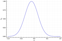
Figure 1: Initial condition $u_{0}^{\text{ref.}}$ depicted on a Chebyshev-Lobatto grid with $500$ points.

4.3 Illustration of the hyperboloidal evolutions: qualitative proof of principle

In order to get some qualitative intuition and illustrate the behaviour of the constructed numerical evolutions of the field $\phi$ in the hyperboloidal scheme, for the four cases of study, we present in Figure 2 the evolution in time $\tau$ of the field evaluated at future null infinity (one endpoint of the grid). In the AdS case we plot the field at the horizon (after rescaling the field by $\sigma$, it only makes sense to show the waveform at the event horizon $\sigma=1$). That is, this is the field an observer at null infinity (or at the horizon in the AdS case) would measure.

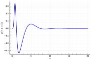
(a) Pöschl-Teller

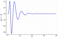
(b) Schwarzschild-dS

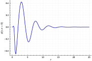
(c) Schwarzschild

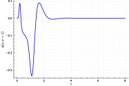
(d) Schwarzschild-AdS

Figure 2: Panels (2a), (2b), (2c) and (2d) are waveforms at future null infinity and at the event horizon for the AdS case (timeseries at a boundary of the Chebyshev-Lobatto grid).

Since the Gaussian initial condition is initially very small at the boundary of the interval, the timeseries is initially flat and close to zero during a very short time, then it increases abruptly, oscillates until it reaches its peak and finally decreases, the signal being dominated at late times by the fundamental mode in the absence of tails (notice the fundamental mode in the Pöschl-Teller case is a constant function of $x$ illustrated later on panel 6a).

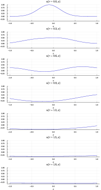
(a) Pöschl-Teller ($V_{0}=b=1$)

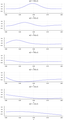
(b) Schwarzschild-AdS ($r_{h}=R=1$)

Figure 3: . Panels (3a) and (3b) show the early time evolution of the field $\phi$ as a function of $x$ (or $\sigma$) at different instants $\tau$. Panel 3b shows the field after its rescaling with $\sigma$ to impose reflexive boundary conditions at $\sigma=0$.

We provide a different view of the field in Figure 3 that aims at verifying a posteriori that the boundary conditions are well-implemented, the field must be purely outgoing at the edges of the interval.

Two observations are in order:

• Pöschl-Teller case We observe that the field is going out in both directions and becomes apparently flat (is dominated by the fundamental mode) after $\tau\approx 1.8$ on 3a, this time corresponds to the minimum of $\phi(x=1,\tau)$ according to 2a.

• Schwarzschild-AdS case The time evolution on panel 3b is obtained using the DAE scheme (125) in particular, the initial condition is different due to the rescaling $u_{0}=\sigma\widetilde{u_{0}}$. Qualitatively, the AdS boundary acts as a box at $\sigma=0$, the amplitude of the signal 2d relative to the maximum of the intial condition on 3b is much higher compared to Pöschl-Teller because it can only dissipate energy at the event horizon.

5 Spectral QNM expansions

After the previous qualitative illustration of the hyperboloidal time evolutions, we now proceed to a systematic study of the comparison of this ‘time-domain’ evolutions with the ‘frequency-domain’ evolutions provided by the asymptotic Keldysh resonant expansions discussed in section 2. We do this for our four cases of study, starting with the numerical construction of spectral elements, namely the QNM frequencies and the QNM functions, as eigenvalues and eigenfunctions on the associated spectral problem, respectively. With these elements at hand, we then proceed to the assessment of the Keldysh expansions by calculating the amplitude coefficients $\mathcal{A}_{n}$ and $a_{n}$, by addressing the contribution of overtones to the waveform and the presence of tails in the Schwarzschild case. The systematic comparison of the time-domain and frequency-domain calculation will serve to assess and validate the latter and, simultaneously, to provide a form of convergence test for the former.

5.1 Keldysh QNM expansion : cases of study

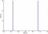
(a) Pöschl-Teller

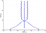
(b) Schwarzschild-dS

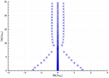
(c) Schwarzschild

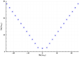
(d) Schwarzschild-AdS

Figure 4: . Panels (4a), (4b), (4c) and (4d) are spectra of the cases of study. These figures are made using $N=500,400,600$ and $400$ respectively.

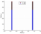
(a) Pöschl-Teller

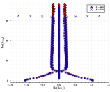
(b) Schwarzschild-dS

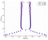
(c) Schwarzschild

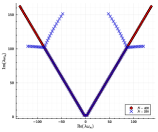
(d) Schwarzschild-AdS

Figure 5: . Panels (5a), (5b), (5c) and (5d) are spectra of the cases of study for different values of $N$.

5.1.1 QNM spectral problem.

In a first step, we solve numerically the spectral problems (9), obtaining the numerical approximations to the QNM frequencies (eigenvalues) $\omega_{n}$, and the numerical approximations $\bm{v}_{n}$ and $\bm{\alpha}_{n}$ to the right- and left-eigenvectors $v_{n}$ and and $\alpha_{n}$, respectively.

As an illustration of the result, Figure 4 provides a spectral follow-up to the time-domain Figures 2 and 3, by presenting a view of the QNM spectra upon which we are going to construct out spectral discussion. Figure 6 shows the first eigenfunctions for the 4 cases of study, we observe that the eigenfunctions reach their maximum at null infinity.

Some general comments are in order:

• Labelling of QNMs. Regarding the labelling of QNMs, given the particular structure of the here studied QNM spectra in the complex plane, each eigenvalue $\omega^{\pm}_{n}$ (in a given QNM branch $\omega^{\pm}_{n}$) is labelled by $n$ and ordered by increasing imaginary part $\mathrm{Im}{\left(\omega_{n}^{\pm}\right)}$.

• General description of spectra. Pöschl-Teller and Schwarzschild panels, respectively panel 4a and panel 4c, simply recover the results in [33]. Even if they are not QNMs, note that in the Schwarzschild case we have kept the eigenvalues corresponding to the discretization of the ‘branch cut’. They do not converge when ‘$N$ increases, but we keep them in the discussion for later convenience. Regarding the asymptotically dS and AdS cases, there is a dependence on the choice of the cosmological constant $\Lambda$. Rather than a systematic study of the dependence on this parameter, we perform here a ‘proof of principle’ calculation by choosing some particular $\Lambda$. In particular, in the asymptotically dS case, the high QNM overtones in panel 4b have a slightly oscillating behavior that depends on the chosen cosmological constant ($\Lambda=0.07$ here). Choosing a higher cosmological constant that is close to the Nariai limit $\Lambda_{\text{Nariai}}=1/9$ seems to reduce these oscillations. Generically speaking, we need to use a high grid size $N$ in the Schwarzschild and Schwarzschild-dS cases so that we can capture the structure of the overtones which are only revealed high in the complex plane.

• Convergence of the QNM frequencies. The convergence of these QNM $\omega_{n}$’, cast as eigenvalues of the appropriate non-selfadjoint operator corresponding to each potential, has been studied in the literature (cf. e.g. [33, 54]). For the purpose of the present discussion, we consider the straightforward (qualitative) test of assessing which $\omega_{n}$’s remain stable when $N$ increases. Specifically, we calculate $\omega_{n}$’s for different resolutions and keep only those that coincide when calculated with the different resolutions. For the sake of clarity in Figure 5 we show the calculation with two different resolutions $N_{1}<N_{2}$, and we keep only those eigenvalues coinciding for both resolutions. Since further increasing the resolution in $N$ does not change the coefficients already stabilised, we take this as a criterion of convergence.

  The Schwarzschild case is however particularly delicate, among our cases of study, something with some impact in the later Keldysh expansion. The branch cut in panel 4c is excluded from the convergence test in panel 5c since these eigenvalues do not converge with $N$ (unlike the de Sitter modes in panel 5b). Their existence seems to heavily influence the actual Schwarzschild QNMs, even those that are not very high in the complex plane. As a consequence, it becomes more subtle to compute a QNM expansion out of a truncated sum of modes that have converged.

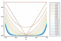
(a) Pöschl-Teller

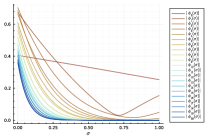
(b) Schwarzschild-dS

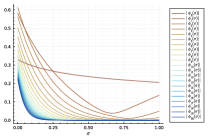
(c) Schwarzschild

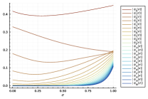
(d) Schwarzschild-AdS

Figure 6: . Panels (6a), (6b), (6c) and (6d) show the first 21 eigenfunctions $\phi_{n}$ for each case of study. The eigenfunctions have been normalized using the energy norm (see 6.1 and [33]).

5.1.2 Calculation of the Keldysh expansion.

Once we have calculated numerically the spectral elements $\omega_{n}$, $v_{n}$ and $\alpha_{n}$, and given our choice of ‘proof of principle’ initial data $u_{0}$, we can make use of the expressions discussed in section 2 and summarised at the end of the article in section 7. Specifically, we have all the elements to make use of later expressions (144 and (148) to construct the Keldysh expansions

$$u(\tau,x) \sim \sum_{n}e^{i\omega_{n}\tau}a_{n}v_{n}(x)=\sum_{n}{\cal A}_{n}(x)e^{i\omega_{n}\tau}\ .$$ (127)

The individual contribution of each quasinormal mode in the Keldysh QNM expansion is therefore given by $\mathcal{A}_{n}(x)e^{i\omega_{n}\tau}=a_{n}v_{n}(x)e^{i\omega_{n}\tau}$. The coefficients $\mathcal{A}_{n}(x)$ are agnostic to the particular prescription in section 2 to compute them (either the use of the transpose $L^{t}$ or rather the adjoint $L^{\dagger}$, the chosen normalisation of $v_{n}$ and $\alpha_{n}$, et cetera), they only depend on the choice of slicing and the compactified coordinate $x$. Conversely, the coefficients $a_{n}$ are independent on $x$ but rely on the normalization of the eigenfunctions $v_{n}$, and therefore on the choice of the scalar product. We will come back to this latter point below in section 6.1 and, at this point, we rather focus on presenting the coefficients ${\cal A}_{n}^{\infty}$ of the time series

$$u(\tau,x_{{I}^{\infty}})\sim\sum_{n}{\cal A}_{n}^{\infty}e^{i\omega_{n}\tau}\ ,$$ (128)

that an observer at null infinity ${I}^{\infty}$ would observe, and that are independent of the chosen hyperboloidal foliation . The interest of the Keldysh approach is that of providing a straight-forward spectral algorithm for calculating the time series (128) for given initial data $u_{0}(x)$:

• Solve the spectral problem: this produces the set $\{\omega_{n},v_{n}(x),\alpha_{n}(x);\forall n\in\mathbb{N}\}$.

• Calculate the coefficients $a_{n}$ of the Keldysh expansion: given $u_{0}(x)$, simply evaluate $a_{n}=\langle\alpha_{n}(x),u_{0}(x)\rangle$.

• Calculate the coefficients ${\cal A}_{n}(x)$ of the Lax-Phillips expansion: simply evaluate ${\cal A}_{n}(x)=a_{n}v_{n}(x)$.

• Evaluate ${\cal A}_{n}^{\infty}$: the coefficients of the time-series (128) are simply given by evaluating ${\cal A}_{n}(x)$ at null infinity, that is ${\cal A}_{n}^{\infty}={\cal A}_{n}(x_{{I}^{\infty}})$.

Such coefficients $\mathcal{A}_{n}^{\infty}$ (corresponding to the considered initial data in (126), illustrated in Figure 1 and giving rise to the time-evolutions in Figures 2 and 3 for the different spacetimes) are presented in in Figure 7, namely their moduli $|\mathcal{A}_{n}^{\infty}|$. Before proceeding to the comparison with the time-domain waveforms, we comment below on the convergence of these $\mathcal{A}_{n}^{\infty}$’s.

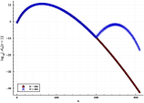
(a) Pöschl-Teller

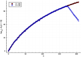
(b) Schwarzschild-dS

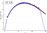
(c) Schwarzschild

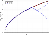
(d) Schwarzschild-AdS

Figure 7: . Panels (7a), (7b), (7c) and (7d) show the modulus of the coefficients $\mathcal{A}_{n}$ at null infinity (or the event horizon in the Schw.-AdS case) for the cases of study. The modes are labelled by $n$ and ordered by increasing imaginary part.

5.1.3 Convergence and growth of coefficients in the Keldysh expansion.

We proceed methodologically as we have done above in section 5.1.1, when considering the convergence of QNM frequencies $\omega_{n}$’s. We focus on the $\mathcal{A}_{n}^{\infty}$ coefficients, although the same analysis can be done for the $a_{n}$’s for a given choice of normalization of $v_{n}$ and $\alpha_{n}$ (see later in section 6.1).

The systematics of the convergence of the $\mathcal{A}_{n}^{\infty}$’s, as the grid resolution $N$ increases, is apparent from Figure 7. As with the QNM frequencies, there is always a clear threshold $n_{T}$ such that for $n<n_{T}$ the $\mathcal{A}_{n}^{\infty}$’s corresponding to two resolutions $N_{1}$ and $N_{2}$ overlap and for $n>n_{T}$ the coefficients split. Specifically, the splitting occur at: i) $n_{T}\approx 200$ for Pöschl-Teller in panel 7a, ii) $n_{T}\approx 172$ for Schwarzschild-dS in panel 7b, iii) $n_{T}\approx 128$ for Schwarzschild in panel 7c, i) $n_{T}\approx 43$ for Schwarzschild-AdS in panel 7d. An important point to note is that, as it is was in the case of the QNM frequencies, the assessment of the convergence of the $\mathcal{A}_{n}^{\infty}$’s for asymptotically flat Schwarzschild is more delicate than in the other cases, as a consequence of the presence of the spurious eigenvalues corresponding to the discretised branch cut, making the construction of the Keldysh resonant expansion more subtle.

We comment now on the growth of the coefficients $\mathcal{A}_{n}^{\infty}$. This, of course, depends critically on the chosen initial data $u_{0}$. Here we consider our ‘reference’ Gaussian initial data in (126) and, therefore, the discussion below is not meant to refer to the generic physical case. This specific case rather provides a ‘proof of principle’ of the concepts and tools we are studying and, in particular, the following discussion is indeed needed for the later comparison with the time-domain results in subsection 5.2.

In the case of Pöschl-Teller in panel 7a, coefficients $\mathcal{A}_{n}^{\infty}$ reach a maximum around $n\approx 125$ and then decrease. In the asymptotically de Sitter and Anti-de Sitter cases, respectively in panel 7b and panel 7d, we get a monotonic increasing profile but we cannot rule out the possibility that the coefficients decrease if the resolution of the grid is high enough to capture overtones higher in the complex plane. Regarding the Schwarzschild case 7c, it exhibits a maximum and a decreasing (averaged) trend as $n$ increases, as in Pöschl-Teller, before the $\mathcal{A}_{n}^{\infty}$’s at different resolutions split in two directions. However, considering individual $\mathcal{A}_{n}^{\infty}$ coefficients, we observe the same type of fluctuations that we had with the spectrum 5c and the individual amplitude coefficients of these high overtones is more difficult to assess.

As commented above, no conclusions about realistic initial data should be drawn. However this test is quite remarkable in the sense that it shows that coefficients $\mathcal{A}_{n}^{\infty}$ can be reliably calculated for data containing very high overtones and that, in spite of theis non-trivial behavior in $n$ (even monotonically increasing, as in the Schwarzschild-dS and Schwarzschild-AdS cases), the convergence properties of the resulting asymptotic series are surprisingly good. Indeed, as we will see below in section 5.2, the comparison with the time-domain signal indicates a very good behaviour of the QNM series, with high overtones playing a key role in the accurate reconstruction at early times. Indeed, the convergence properties of the series are “unexpectedly” good , something that will be studied in detail in [30].

5.2 Comparison between time and frequency domain evolutions

We attain in this section the central point of this work: the direct comparison between the time domain signal, constructed from the direct time integration of Eq. (29), and the spectral QNM expansion (2.2), built for the initial data $u_{0}$ in (29). As already indicated, we stay at a “proof of principle” perspective, providing the basic elements of the comparison and building on the specific initial condition (1) employed in the previous section LABEL:s:time_evol to explore the different black hole asymptotics. A more detailed and extended analysis, in particular concerning larger classes of initial data, is leaved for a future work.

We start from the asymptotic expansion (2.2) and introduce the finite truncated QNM expansion with the first $N_{\mathrm{QNM}}$ QNMs (for each branch $\omega_{n}^{\pm}$), that we denote as $u^{\mathrm{QNM}}(\tau,x)$

$$u^{\mathrm{QNM}}(\tau,x)=\sum_{n=0}^{N_{\mathrm{QNM}}}\mathcal{A}^{\pm}_{n}(x)e^{i\omega^{\pm}_{n}\tau}.$$ (129)

Figure 8 shows the times-series corresponding to the evaluation if $u(\tau,x)$ at null infinity (Pöschl-Teller, Schwarzschild), the cosmological horizon (Schwarzschild-dS) or the horizon (Schwarzschild-AdS) for both the time-domain solutions (in blue) presented in section LABEL:s:time_evol and the corresponding truncated QNM expansions (in red), calculated accordingly to the Keldysh prescription. Regarding the time-domain signal, it corresponds exactly to the panels in Figure 2, but in a logarithmic plot.

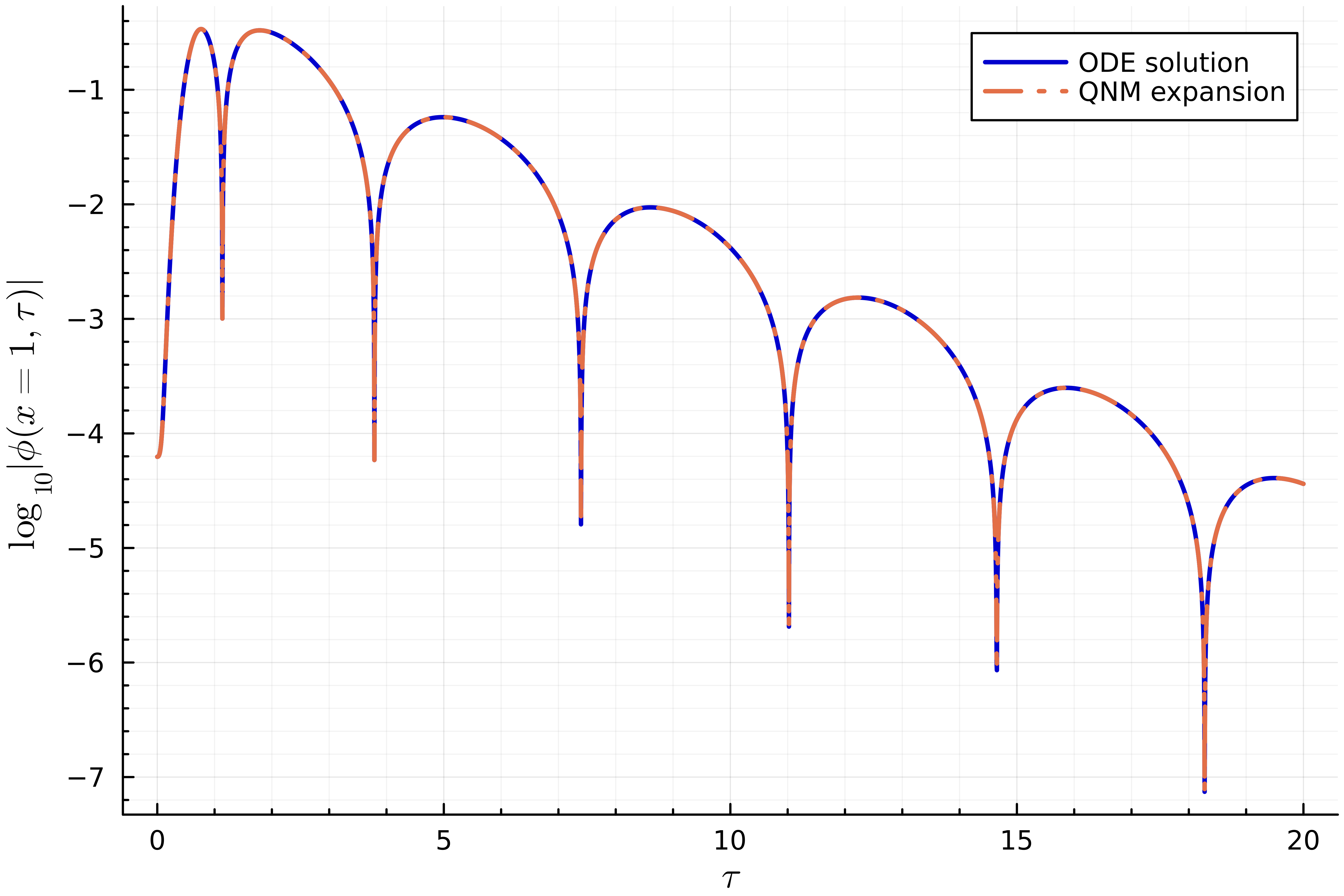
(a) Pöschl-Teller

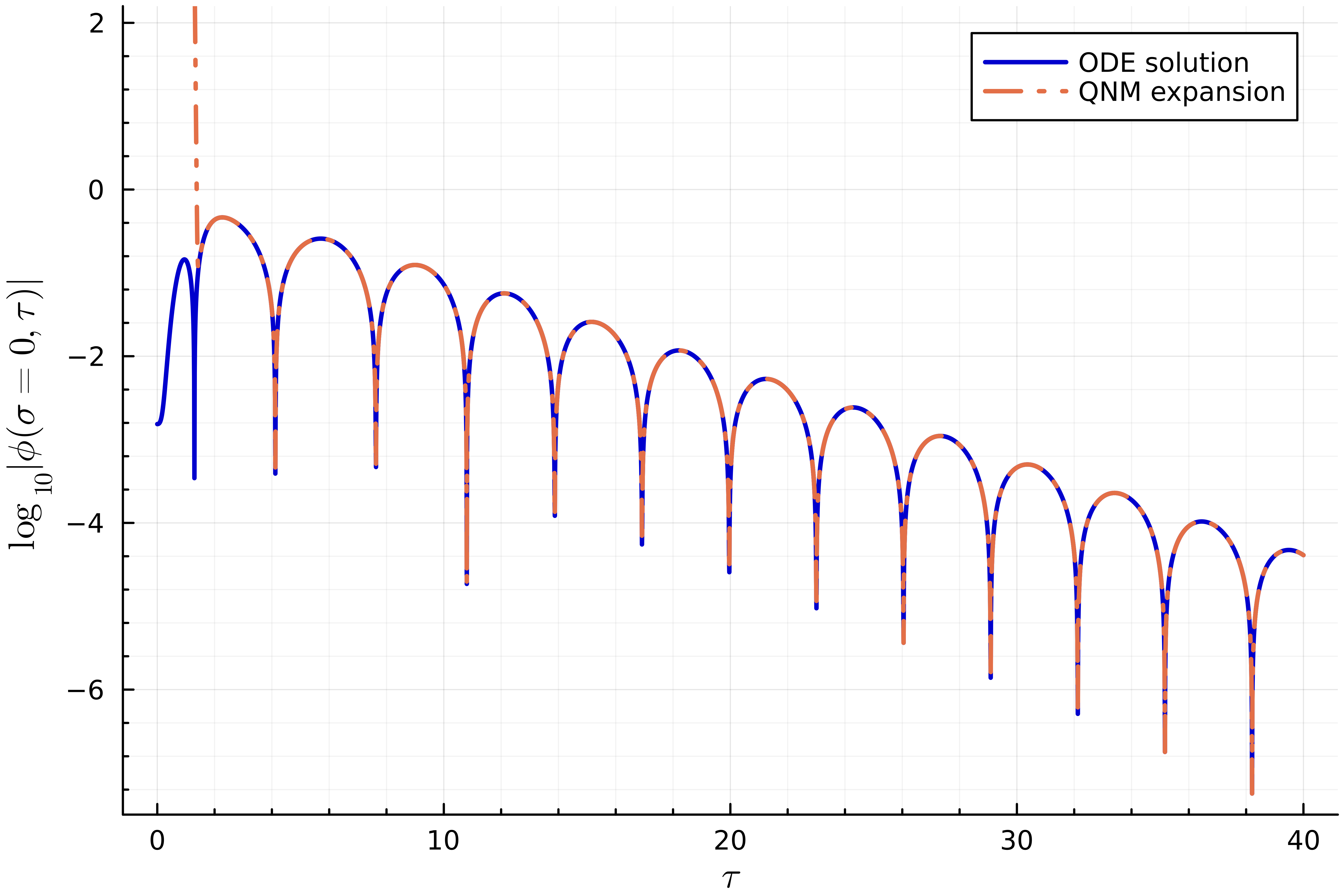
(b) Schwarzschild-dS

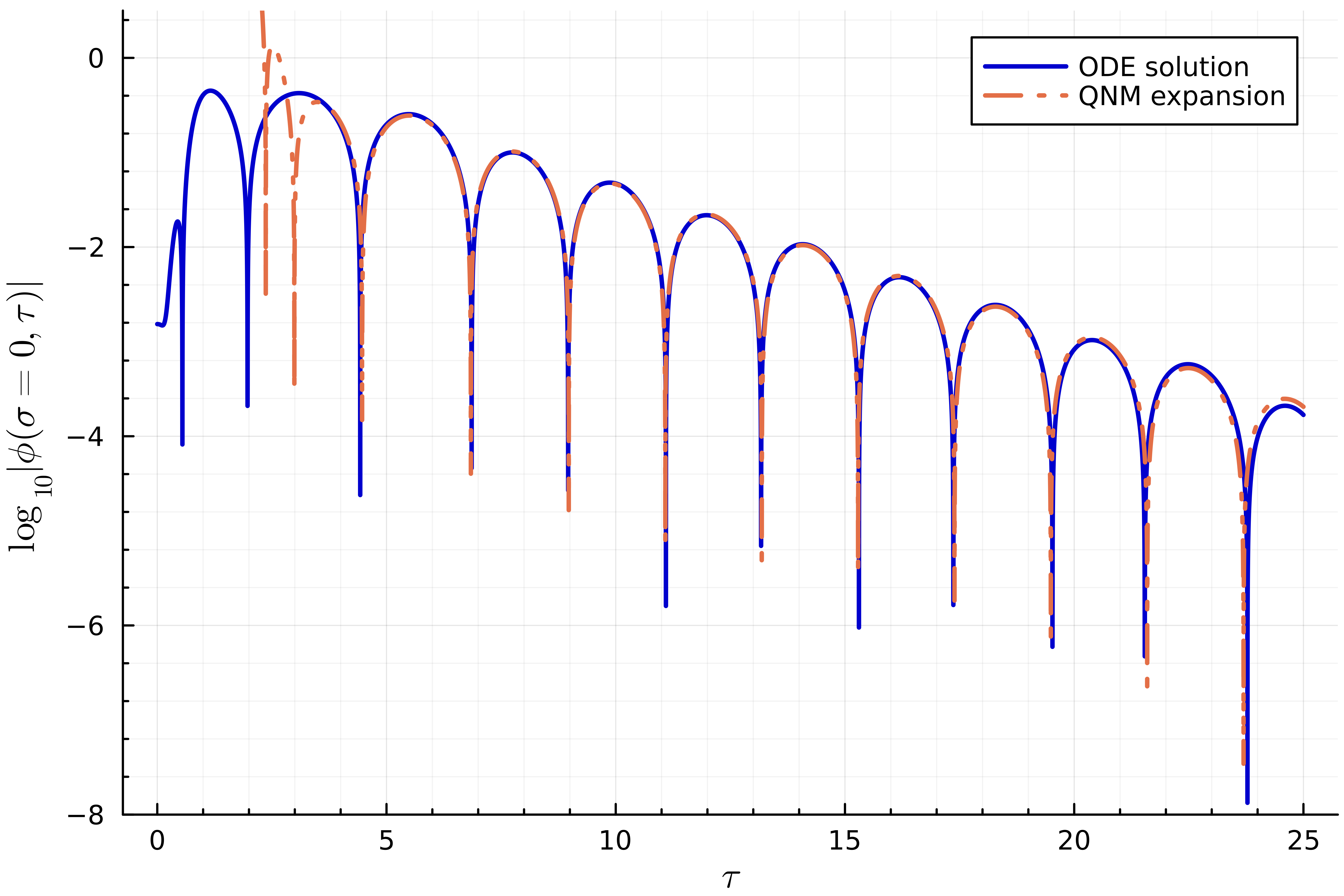
(c) Schwarzschild

(d) Schwarzschild-AdS

Figure 8: . Panels (8a), (8b), (8c) and (8d) show both the ODE/DAE solution and the numerical resonant expansion.

There are two parameters to control the Keldysh QNM expansions in Fig. 8: on the one hand, the number $N_{\mathrm{QNM}}$ determining the QNMs employed in each truncanted QNM expansion (namely $N_{\mathrm{QNM}}+1$ QNMs) and, on the other hand, the size $N$ of the Chebyshev-Lobatto grids employed in the discrete approximations $\bm{u}^{\mathrm{QNM}}$ of $u^{\mathrm{QNM}}$ (namely using $N+1$ Chebyshev-Lobatto collocation points). Regarding $N_{\mathrm{QNM}}$ this is given by the number of QNMs whose coefficients ${\cal A}_{n}^{\infty}$ in Fig. 7 have already converged. Regarding the grid resolution $N$, it corresponds to the finest grid in used Fig. 7. In Fig. 9 we plot the absolute difference between the time domain and QNM time-series, namely $\left|u(\tau,x_{\mathrm{boundary}})-u^{\mathrm{QNM}}(\tau,x_{\mathrm{boundary}})\right|$.

We comment below on the four studied cases :

• Pöschl-Teller case ($N_{\mathrm{QNM}}=310$, $N=500$): the early times times-series is very accurately described by the QNM expansion and the error is always smaller than the tolerance in the time-domain evolution, the first points of the timeseries 9a even suggests that the error might be below $10^{-40}$, which is coherent with the value of the highest correct overtone on 5a.

• Schwarzschild-dS case ($N_{\mathrm{QNM}}=205$, $N=600$): for the chosen number $N_{\mathrm{QNM}}$ of QNMs, the early times of the signal presents a huge error which decreases quickly and gets below the numerical precision of the time-evolution solver. The oscillations appearing in Fig. 9 correspond to artifacts of the discretization scheme of the time derivatives determined when choosing the time-evolution solver’s algorithm.

• Schwarzschild-AdS ($N_{\mathrm{QNM}}=69$, $N=400$): very similar qualitative bevahior to the Schwarzschild-dS case, although with a much faster decay that is captured with a significantly lower number of QNMs

• Schwarzschild ($N_{\mathrm{QNM}}=30$, $N=600$): unlike the previous three cases, the error in the case of Schwarzschild is not limited by the time-domain solver. We will comment this case in more detail below in subsection LABEL:S_tails, in particular when looking at late times when the signal is not dominated by QNMs but by tails. The agreement between the time-domain QNM signal and the truncated QNM expansion is nevertheless very good.

We would like to comment on two features in Figs. 8 and 9. The first one concerns fundamentally Pöschl-Teller, Schwarzschild-dS and Schwarzschild-AdS (but also Schwarzschild in a smaller degree). Specifically, as it can be seen in Figs. 8 and 9, the global agreement between the time-domain and the QNM expansion signals is remarkable. The accurate agreement at late times (or intermediate in the case of Schwarzschild) is expected, since the signal is then controlled by slow-decaying QNMs. More interesting is the fact that, as seen in Fig. 9, such accuracy is maintained during most of the whole signal till quite early times. But the truly remarkable feature is that this agreement can be pushed to even earlier times by adding additional QNMs. We address this point in subsection 5.3. The second point concerns specifically Schwarzschild, namely the only case with a “branch cut”, and the tails at late times. We address this in subsection 5.4

(a) Pöschl-Teller

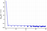
(b) Schwarzschild-dS

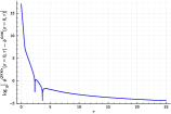
(c) Schwarzschild

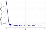
(d) Schwarzschild-AdS

Figure 9: . Panels (9a), (9b), (9c) and (9d) show the difference between the ODE/DAE solution and the numerical resonant QNM expansion. The numerical precision of the solver (the tolerance) is $10^{-20},10^{-15},10^{-15}$ and $10^{-10}$ respectively for the 4 cases under study. We don’t have a precise control over the precision, the solver is a black box for us and it might start with a much high precision for $\tau$ small as the Pöschl-Teller panel suggests.

5.3 The role of overtones: earliest time for the validity of the QNM expansion

As commented above, as we add more and more QNM overtones to the $u^{\mathrm{QNM}}$ in (129) the resulting QNM time-series starts its agreement with the time-domain time series at earlier and earlier times. This is illustrated in Fig. 10 for the Pöschl-Teller (though a similar behaviour occurs in other studied cases): as more and more overtones are added the corresponding colored curves (passing from the red to the blue) smoothly join the time-domain signal (black curve) earlier and earlier. Two comments are in order here, regarding this good performance of the QNMs:

• Control of early dynamics by the QNM spectrum. In the context of a dynamical problem whose infinitesimal time generator is non-selfadjoint (actually non-normal) the control of the evolution by the spectrum is only guaranteed at late times. In principle, to study the early evolution one needs to control not only the spectrum but also the resolvent far from the spectrum, something that can be cast in terms of the pseudospectrum in a non-modal analysis approach to the dynamics [58, 59, 55]. In the generic case, transients involving an initial growth of the signal and controlled by the pseudospectrum far from the spectrum do appear. In contrast with this situation, the behaviour illustrated in Fig. 10 (that was originally identified in [3, 52]) seems to indicate that the QNM spectrum indeed controls the dynamics since very early times. Although this may be surprising in our non-selfadjoint setting, it is indeed consistent with the vanishing of the so-called numerical abscissa $\omega(L)$ in [32] (see also [10], [11], [12] and [29]).

• Initial time $\tau^{\mathrm{QNM}}_{\mathrm{init}}$ of validity of the QNM expansion. Given that adding more and more overtones we reach earlier and earlier times, a natural question to ask is whether there exists an earliest time $\tau^{\mathrm{QNM}}_{\mathrm{init}}$ after which the time-domain and the QNM signals “coincide”. This problem has been addressed in [3] leading to an answer in the affirmative. More specifically they propose that, for a given initial data $u_{0}(x)$ and for each time-series at fixed $x_{\mathrm{t-s}}$, i.e. $u(\tau,x=x_{\mathrm{t-s}})$, such time is given by $\tau^{\mathrm{QNM}}_{\mathrm{init}}(x_{\mathrm{t-s}})=\nu(x_{\mathrm{t-s}})$, where $\nu(x_{\mathrm{t-s}})$ is the “growth rate of excitation coefficients” $\nu(x)=\lim_{n\to\infty}\frac{{\cal A}_{n}(x)}{|\omega_{n}|}$. Interestingly, in all cases studied , our results suggest $\nu(x_{b}=0$). This follows from the linear growth of the $\omega_{n}$ with n (cf. Figs. 4 and 5) and the convexity of ${\cal A}_{n}(x_{b})$ in Fig. 7.

  A related but different question is the following: given an initial data $u_{0}$ and a fixed $\tau=\tau_{o}$, does the asymptotic QNM series converges in the sense of a series? In other words, can we write

  $$u(\tau_{o},x)=\sum_{n=0}^{\infty}e^{i\omega_{n}\tau_{o}}{\cal A}_{n}(x)\ ,$$ (130)

  as an actual convergent series of functions and not just as an asymptotic series? To address this question we can rewrite the asymptotic series expansion (2.2) as

  $$u(\tau,x) = \sum_{n=0}^{N_{\mathrm{QNM}}}e^{i\omega_{n}\tau}\langle\alpha_{n},u_{0}\rangle v_{n}(x)+E_{N_{\mathrm{QNM}}}(\tau;u_{0})$$

  $$= u^{\mathrm{QNM}}(\tau,x)+E_{N_{\mathrm{QNM}}}(\tau;u_{0})$$

  with $$||E_{N_{\mathrm{QNM}}}(\tau;u_{0})||\leq C(N_{\mathrm{QNM}},L)e^{-\kappa N_{\mathrm{QNM}}\tau}||u_{0}||\ .$$ (131)

  where $u^{\mathrm{QNM}}(\tau,x)$ in (129) provides now a partial sum of the series and the form $a_{N_{\mathrm{QNM}}}=\kappa N_{\mathrm{QNM}}$ for $a_{N_{\mathrm{QNM}}}$ in(2.2) is consistent with the BH QNM asymptotics, inferred from Figs. 4 and 5) and leading to a BH Weyl law that extend [34] (see C). In general, the asymptotic series (ii)) cannot be guaranteed to be convergent due to the fact that $C(N_{\mathrm{QNM}},L)$ does not provide a uniform bound for error. Then, for a given $\tau$, the assessment of the convergence of the series amounts to controlling the growth of $C(N_{\mathrm{QNM}},L)$ with $N_{\mathrm{QNM}}$. Preliminary results [30] indicate that, for the initial data here employed, there exists a time $\tau_{o}$ such that for $\tau>\tau_{o}$ the series is indeed convergent.

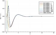
(a) Adding overtones to the truncated QNM expansion

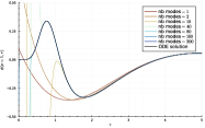
(b) Early $\tau$ view (zoom)

Figure 10: . Panels (10a) show the truncated QNM expansion in the Pöschl-Teller case with a variable number of modes. We start with only the fundamental mode and we finish with $200$ modes which corresponds to a dark blue curve hidden behind the black one.

5.4 Schwarzschild case : tails from Keldysh expansions

We address now the second point raised at the end of subsection 5.2, namely the tails of Schwarzschild at late times.

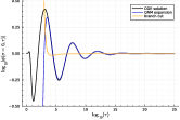
(a) Waveform at future null infinity $\phi(\tau,\sigma)|_{\sigma=0}$

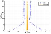
(b) Eigenvalue plot

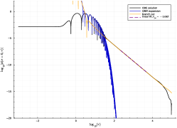
(c) Waveform $\phi(\tau,\sigma)|_{\sigma=0}$ on a log-log plot

Figure 11: . In the Schwarzschild case, with $\ell=2$ and $N=600$, we illustrate how the contribution of the branch cut and of the QNMs dominate the waveform one after the other. Initially, both of these curves contribute to the signal, then the ringdown starts at $\tau=4$ and is dominated by QNMs, after that when the QNMs get small enough, the power-law regime dominates for a long time before it vanishes and an asymptotic exponential decay takes place due to the finite number of modes in the numerical sum. We performed a linear fit to estimate the power law tail $\tau^{\beta_{fit}}$.

A stark difference between the Schwarzschild case and the other three cases is that its null infinity is less regular than its black hole horizon. In the hyperboloidal scheme this translates into the fact the function $p(x)$ in $L_{1}$ (cf. Eqs. (3.2) and (71) vanishes quadratically at future null infinity, whereas at the horizon it vanishes linearly (as it does in all other three cases at outgoing boundaries). As a consequence, the spectrum of the operator $L$ contains, apart from the discrete QNM eigenvalues, a continuous part along the positive imaginary axis (known as “branch-cut” in the scattering resonance approach) that is responsible for a power-law tail of the waveform at late times. After discretization, this branch-cut gives rise to (non-convergent) eigenvalues, as it can be seen in Figs. 4 and 5c, along the imaginary axis.

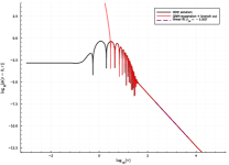
(a) $\ell=2$

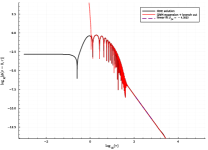
(b) $\ell=3$

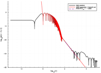
(c) $\ell=4$

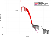
(d) $\ell=5$

Figure 12: . Panels (12a), (12b), (12c) and (12d) show the polynomial tails we get from adding the branch cut modes to the QNM expansion for different angular $\ell$’s. The linear fit to estimate the power law tail time decay $\sim\tau^{\beta_{fit}}$ demonstrates the Price law.

When considering the spectral decomposition of the scattered field, one of the assumptions in the discussion of the Keldysh expansion in section 3.2 was the discreteness of the spectrum of $L$. As shown in previous section, this has provided excellent results for the part of the signal dominated by QNMs. However, it also means that it is not a tool well adapted to the tails, encoded in the continuum branch cut. In this setting it comes as an unexpected result the fact that the naive application of the Keldysh scheme also to the branch cut (i.e. beyond its regime of validity) provides with an excellent account of the tail part of the signal. More specifically: the straightforward application of the Keldysh scheme to the (non-convergent) eigenvalues corresponding to the discretization of the branch cut does provide an accurate description of the late tails.

The latter is, in principle an unexpected result that could be tried to be understood in terms of a Riemann sum approximation of the Bromwich integral that one has to calculate along the branch cut to account for the tails (see e.g. [3]). However a simpler and more direct explanation is given in terms of the discussion presented in B, were the dynamical evolution is obtained by applying the discretised evolution operator $e^{i\tau L}$ on the initial data $u_{0}$ . In the following we comment on the main points regarding tails in this Keldysh approach:

• Polynomial tails from a Keldysh sum over “branch-cut eigenvalues”: spectral separation of QNM and tails. Fig. 11 shows the calculation the respective contributions of QNMs and branch-cut to the scattered field. Panel 11a shows the time-domain waveform (black) and the contributions of the QNM expansions (blue) and branch cut (orange). The corresponding eigenvalues from which QNM and tail signals are calculated (by applying exactly the same Keldysh algorithm) are shown in panel 11b, with the same code of colors. Finally panel 11c shows a log-log plot where the power-law nature of the tails is apparent.

• Price law. Figure 12 presents the signal (in red) resulting from the sum of the QNM expansion and the signal from the branch cut eigenvalues. This is done for various $\ell$’s. In all cases the time-domain signal is accurately fitted. A robust demonstration of the good convergence behaviour of the Keldysh scheme is the recovery of the Price law, namely the late time decay $\sim\tau^{-(\ell+1)}$.

• Numerical convergence of the tail. Fig. 13 shows how increasing the numerical resolution, by taking larger $N$’s in the Chebyshev-Lobatto’s grid, permits to get correspondingly larger times for the tail. This provides a qualitative demonstration of the tail convergence in the numerical scheme.

The bottom line is that the Keldysh scheme combined with the Chebyshev-psedospectral discretisation provides a simple, efficient and accurate algorithm for the calculation of Schwarzschild tails. The Keldysh prescription underlines the spectral separation of QNMs and tails contributions.

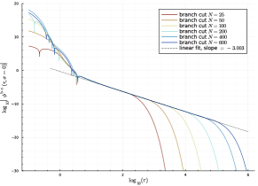
Figure 13: . We compute the expansion over the branch cut eigenvalues as a function of $\log_{10}(\tau)$ for several gridsizes $N\in\{25,50,100,200,400,600\}$ in the Schwarzschild case ($\ell=s=2$).

6 Regularity and excitation coefficients

6.1 QNM expansions and scalar product

We have insisted on the agnostic nature of the Keldysh QNM expansion and of the “expansion coefficient” functions $\mathcal{A}_{n}(x)$ in section 5.1.2. However, on the one hand, there can be physical scenarios in which a QNM expansion of the form given in (52), that we rewrite here as

$$u(\tau,x)\sim\sum_{n}a_{n}\hat{v}_{n}(x)e^{i\omega_{n}\tau}\ ,$$ (132)

is of interest . Such a QNM is in the spirit of the normal modes expansion (6), where expansion constant coefficients $a_{n}$ are defined. Writing the QNM expansion (132) amounts to have a physically well motivated scalar product $\langle\cdot,\cdot\rangle_{{}_{G}}$. The physical meaning of the corresponding coefficients $a_{n}$’s would be encoded in the physical content of the chosen scalar product. On the other hand, from a structural perspective, the choice of scalar product is intimately related to the regularity aspects of QNMs, known to be a key element in the definition (and instability) problem of QNMs, as shown by Warnick [62, 63] (see also [31]).

If we accept the potential interest of expression (132), we are left with the freedom to choose the scalar product to normalize the eigenfunctions $v_{n}$ and compute $a_{n}$, something that translates into exploring different scalar products to control the behaviour of the excitation coefficients, in particular high overtone Given the dependence of the $a_{n}$ on the scalar product $\langle\cdot,\cdot\rangle_{{}_{G}}$ is natural to denote then as $a_{n}^{G}$.

In summary, whereas the goal of the previous section 5.1.3 was to introduce and assess the coefficients of the time-series QNM expansion at ${I}^{+}$ or at the black hole event horizon (this amounting to fix the spatial coordinate $x$ (or $\sigma$) at the boundary of the interval and considering the expansion), we now characterize the QNM expansion as a sum over the normalized eigenfunctions $\hat{v}_{n}(x)=\frac{v_{n}(x)}{\left\|v_{n}\right\|_{{}_{G}}}$: as we explained in section 5.1.2 we trade coefficients ${\cal A}_{n}(x)$’s that depend on $x$ for coefficients $a_{n}^{G}$’s that depend on the scalar product. The relation between the $a_{n}$’s and the norm $\left\|v_{n}\right\|_{{}_{G}}$ is given by $a^{G}_{n}=a_{n}\left\|v_{n}\right\|_{{}_{G}}$

$$\!\!\!\!\!\!\!\!\!\!\!\!\!\!\!\!{\cal A}_{n}(x)=a_{n}v_{n}(x)=a_{n}\left\|v_{n}\right\|_{{}_{G}}\frac{v_{n}(x)}{\left\|v_{n}\right\|_{{}_{G}}}=a_{n}\left\|v_{n}\right\|_{{}_{G}}\hat{v}^{G}_{n}(x)=a^{G}_{n}\hat{v}^{G}_{n}(x)\ .$$ (133)

In this section we limit ourselves to present behaviour of such $a^{G}_{n}$’s under some particularly motivated choices of scalar product. We consider the case of the “energy scalar product” $\langle\cdot,\cdot\rangle_{{}_{E}}$, employed in the study of QNM stability [33, 25], and (a class of) Sobolev spaces $H^{p}$, that are crucial in the control of the regularity in the definition problem of QNMs [63, 9].

6.2 QNM expansion coefficients $a^{E}_{n}$ in the energy norm

As commented above, this scalar product is of relevance in the discussion of QNM (in)stability, that can be accounted in terms of the so-called pseudospectrum [33]. For later comparison with $H^{p}$-Sobolev scalar products we present in Fig. 14 the energy pseudospectrum for the Pöschl-Teller case.

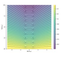
(a) Pöschl-Teller

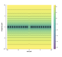
(b) self-adjoint case

Figure 14: . Panel (14a) show the energy pseudospectrum in the Pöschl-Teller case. Panel (16d) shows test provided by the self-adjoint case $L_{2}=0$. $N=30$ for both panels.

More generally, it is the scalar product defining the natural norm to be employed in the PDD initial value problem (29), where the energy of the solution is controlled. In the notation of section 3.2, it writes

$$\langle u_{1},u_{2}\rangle_{{}_{E}}=\Big{\langle}\begin{pmatrix}\phi_{1}\\ \psi_{1}\end{pmatrix},\begin{pmatrix}\phi_{2}\\ \psi_{2}\end{pmatrix}\Big{\rangle}_{{}_{E}}=\frac{1}{2}\hskip-2.84526pt\int_{a}^{b}\hskip-2.84526pt(w(x)\bar{\psi}_{1}\psi_{2}+p(x)\partial_{x}\bar{\phi}_{1}\partial_{x}\phi_{2}+\tilde{V}(x)\bar{\phi}_{1}\phi_{2})dx\ .$$ (134)

and it holds indeed that the square of the norm of the field $u$ gives its energy at the slice $\tau=\mathrm{const}$

$$E_{\tau}(u)=||u||^{2}_{{}_{E}}\ .$$ (135)

Figure 15 presents the coefficients $a_{n}^{E}$ for the QNM expansion of our Gaussian “proof-of-principle” test initial data $u_{0}$ in Eq. (126).

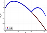
(a) Pöschl-Teller

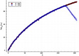
(b) Schwarzschild-dS

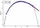
(c) Schwarzschild

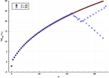
(d) Schwarzschild-AdS

Figure 15: . Panels (15a), (15b), (15c) and (15d) show the modulus of the coefficients $a_{n}$ corresponding to the energy norm. The modes are labelled by $n$ and ordered by increasing imaginary part.

We note that, remarkably, the $a_{n}^{E}$ are very similar to the $\mathcal{A}^{\infty}_{n}$, upon comparing Figures 7 and 15 we notice they are only moved up slightly. From (133), this amounts to $|\hat{v}_{n}(1)|\sim 1$. We explore below the behaviour of $a_{n}^{G}$’s when choosing rather a Sobolev norm.

6.3 Coefficients in the $H^{p}$ Sobolev scalar product

Sobolev norms $H^{p}$ are fundamental in the definition problem of QNMs. They amount to the need of requiring enhanced regularity to QNM eigenmodes in order them provide a discrete set of modes. In this process, from (133) we see that by increasing $p$ in $H^{p}$ coefficients $a_{n}^{H^{p}}$ associated with functions with small scale structure (therefore larger $||v_{n}||_{p}$) are enhanced.

6.3.1 A $H^{p}$ scalar product.

We consider the following $H^{p}$-like scalar product constructed on the energy scalar product and reducing to energy scalar product for $p=0$

$$\langle u_{1},u_{2}\rangle_{{}_{H^{p}}}=\Big{\langle}\begin{pmatrix}\phi_{1}\\ \psi_{1}\end{pmatrix},\begin{pmatrix}\phi_{2}\\ \psi_{2}\end{pmatrix}\Big{\rangle}_{H^{p}}=\sum_{j=0}^{p}\Big{\langle}\begin{pmatrix}\partial_{x}^{j}\phi_{1}\\ \partial_{x}^{j}\psi_{1}\end{pmatrix},\begin{pmatrix}\partial_{x}^{j}\phi_{2}\\ \partial_{x}^{j}\psi_{2}\end{pmatrix}\Big{\rangle}_{E}\ ,$$ (136)

with associated Gram matrix

$${\textbf{G}_{\text{H}^{p}}}=\sum_{j=0}^{p}\left(\begin{array}[]{c|c}\mathbb{D}_{N}^{(j)}&0\\ \hline\cr 0&\mathbb{D}_{N}^{(j)}\end{array}\right)^{t}{\textbf{G}_{\text{E}}}\left(\begin{array}[]{c|c}\mathbb{D}_{N}^{(j)}&0\\ \hline\cr 0&\mathbb{D}_{N}^{(j)}\end{array}\right)\ ,$$ (137)

and leading to the norm

$$\left\|\begin{pmatrix}\phi\\ \psi\end{pmatrix}\right\|_{H^{p}}^{2}:=\sum_{j=0}^{p}\left\|\begin{pmatrix}\partial_{x}^{j}\phi\\ \partial_{x}^{j}\psi\end{pmatrix}\right\|_{E}^{2}$$

that adds the energy norm of the mode and its first $p$ derivatives .

6.3.2 Norm and $H^{p}$-pseudospectrum.

In Fig. 16 we present the pseudospectra for the Pöschl-Teller case calculated with the $H^{p}$ norm, for different values of $p$ (compare with Fig. 14 for the energy norm). The interest of presenting such pseudospectra is twofold.

On the one hand, from a conceptual perspective, they make apparent the link between regularity and definition of QNMs. Indeed, as we increase $p$ we gain control on more and more overtones, as it can be seen in the circular pseudospectral lines around growing overtones. This is consistent with the results by Warnick [63], where QNMs are defined in horizontal bands  of width $\kappa$, in such a way that an $H^{p}$ norm is needed to control the first $p$ bands (see details in [63, 9]). As we can see in Fig. 16, when using a $H^{p}$ norm given in (6.3.1) we make stable the first $p$ QNMs. In order to get control on one additional QNM, the energy norm of one additional derivative must be added, passing from an $H^{p}$ to an $H^{p+1}$ norm. These pseudospectra represent by themselves a non-trivial result (see also [62] for related results ). They are not only consistent with the results in [63] but they permit to clarify the non-convergence issues with the grid-resolution $N$, associated with pseudospectra constructed with the energy norm. More details will be presented in a dedicated work [31].

On the other hand, from a practial perspective in the setting of the present article, the actual construction of pseudospectra in Fig. 16 provides an excellent test (they faithfully recover the band structure in Warnick’s theorem) for the correct implementation of $H^{p}$ norms, a crucial step before calculating the corresponding QNM coefficients $a_{n}^{H^{p}}$.

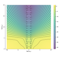
(a) $H^{5}-$pseudospectrum

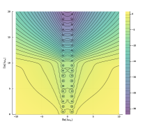
(b) $H^{10}-$pseudospectrum

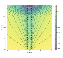
(c) $H^{15}-$pseudospectrum

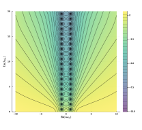
(d) $H^{20}-$pseudospectrum

Figure 16: . Panels (16a), (16b), (16c) and (16d) show the $H^{p}$-pseudospectrum in the Pöschl-Teller case with $p=5,10,15$ and $20$. For both panels $N=30$.

6.3.3 QNM expansion coefficients $a_{n}^{H^{p}}$ in the $H^{p}$ norm.

Norms $H^{p}$ with increasing $p$ are correspondingly more sensitive to the small scale of the functions. As we have commented above (cf. Eq. (133), the use of $H^{p}$ norms enhances coefficients $a_{n}^{H^{p}}$ corresponding to QNM eigenfunctions with more small scale structure. This can be appreciated in Figure 17, where coefficients $a_{n}^{H^{p}}$ with larger $n$ gets bigger as $p$ increases. The results in this section suggests that the use of $H^{p}$ norms can be of interest in the study and understanding of small scale/regularity issues in QNM expansions. This will be developed elsewhere.

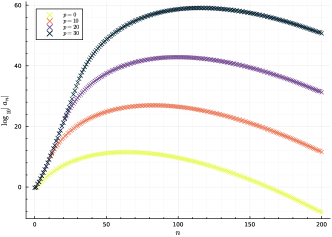
Figure 17: QNM expansion coefficients $a_{n}^{H^{p}}$, for different $H^{p}$ norms, as a function of $n$.

7 Conclusions

In this work we have discussed asymptotic QNM resonant expansions for scattered fields on BH (stationary) spacetimes in an approach that makes key use of hyperboloidal foliations to render the problem in a non-selfadjoint spectral setting where use can be made of a so-called Keldysh expansion of the resolvent.

We have implemented the Keldysh approach to QNM expansions in a set of BH spacetimes with different asymptotics and in the toy-model provided by the Pöschl-Teller potential. This extends to the gravitational setting a tool that has been successfully applied before in optics and mechanical problems [47]. The accuracy of the QNM expansions in the comparison with time-domain signals in this gravitational setting, where dissipation occurs only at the boundaries, is remarkable. Results in this article can be classified in:

• Structural results. We have revisited the discussion of Keldysh QNM expansions in [25], clarifying the role of the scalar product. We conclude:

  • Keldysh QNM expansions only involve ‘dual space-pairing’ notions: specifically, the scalar product is not a structure needed for constructing Keldysh QNM expansions $u(\tau,x)\sim\sum_{n}{\cal A}_{n}(x)e^{i\omega_{n}\tau}$. In particular, no canonical choice of constant $a_{n}$ in $u(\tau,x)\sim\sum_{n}a_{n}v_{n}(x)e^{i\omega_{n}\tau}$ (with $v_{n}$ QNM eigenfunctions) can be made, only the product ${\cal A}_{n}(x)=a_{n}v_{n}(x)$ being defined at this level.

  • Keldysh QNM expansions generalise previous QNM expansion schemes: they extend to arbitrary dimensions (and to more general spectral formulations of the scattering problems) the BH QNM expansion by Ansorg & Macedo. Likewise, it provides a spectral description of Lax-Phillips resonant expansions, adapted to the hyperboloidal scheme.

  • Uniqueness of the QNM time-domain series at null infinity ${I}^{+}$: the time-series $u(\tau)\sim\sum_{n}{\cal A}_{n}^{\infty}e^{i\omega_{n}\tau}$, where $\tau$ is the retarded time at null infinity, is obtained by straightforward evaluation of the Keldysh expansion at ${I}^{+}$, namely ${\cal A}_{n}^{\infty}={\cal A}_{n}(x_{{I}^{+}})$. This would correspond to directly GW detector observational data.

  • Role of the scalar product to determine constant coefficients $a_{n}$: the determination of constants $a_{n}$ requires a scalar product (actually, only a norm) to fix the “size” of QNM eigenfunctions $\hat{v}$. Then we can meaningfully write $u(\tau,x)\sim\sum_{n}a_{n}\hat{v}_{n}(x)e^{i\omega_{n}\tau}$. This is the closest form to self-adjoint normal mode expansions.

  • Choice of scalar product and construction of $H^{p}$-pseudospectra: the choice of scalar product (or, more generally, of non-degenerate quadratic form) is not unique and different choices can be of interests in different contexts. We have explicitly illustrated this by the calculation of Pöschl-Teller pseudospectra with different $H^{p}$-Sobolev norms as well as the associated $a_{n}$’s for a test-bed choice of initial data.

• Particular results in the black hole scattering. We have demonstrated shown that the Keldysh approach to QNMs provides, in the BH case, and efficient and accurate scheme to calculate the QNM expansions. In particular:

  • Comparison of Keldysh QNM expansions and time-domain scattered field. We have explicitly implemented the Keldysh expansion, studied the convergence of expansion coefficients $a_{n}$ and compared with the time-domain evolved field for a family of on test-bed initial data. Results are remarkable even at early times.

  • Keldysh recovery of Schwarzschild’s tails. As an expected result, we have found that the scheme works also beyond its ‘limit of validity’. Specifically, although the Keldysh expansion is only guaranteed to work when applied to discrete eigenvalues, we have found part that its ‘blind’ application to (eigenvalues corresponding to finite-rank approximations of) the ‘branch cut’ successfully construct the late power-law tails, correctly recovering the correct Price law.

  • Early evolution and high overtones. Although the asymptotic expansion is only guaranteed to approach the time-domain signal, at a given (a priori) error, starting from some finite time after the beginning of the evolution (such time being associated with the number of QNMs in the finite-sum approximation), for the class of employed test-bed data we have found that we reproduce accurately the signal at arbitrary early times by including sufficiently high overtones. The contributions of such overtones is large at the spectral level (large $a_{n}$’s) dominating the early signal.

  • High overtones and Weyl law for BH spacetimes with different asymptotics. Given the relevant role of high overtones at early times, we have provided a qualitative test of their distribution in the complex plane by calculating their Weyl’s law. We have found that the QNM counting function presents the correct power-law $N(\omega)\sim\omega^{3}$ independently of the spacetime asymptotics.

7.1 Explicit expressions of asymptotic Keldysh QNM expansions

In order to ease the access to relevant expressions, and at the risk of redundancy, we collect here the relevant expressions for the QNM asymptotic expansions presented in this work.

• Keldysh asymptotic QNM expansion:

  Given the standard spectral problems for the infinitesimal generator of time $L$

  $$Lv_{n}=\omega v_{n}\ \ ,\ \ L^{t}\alpha_{n}=\omega\alpha_{n}\ \ ,\ \ v_{n}\in{\cal H},\alpha_{n}\in{\cal H}^{*}\ ,$$ (138)

  we can write the scattered field evolved from initial data $u_{0}$ as

  $$u(\tau,x) \sim \sum_{n}e^{i\omega_{n}\tau}a_{n}v_{n}(x)\ ,$$ (139)

  with

  $$a_{n}=\left\{\begin{array}[]{lcl}\displaystyle\frac{\langle\alpha_{n},u_{0}\rangle}{\langle\alpha_{n},v_{n}\rangle}&,&\ \ \hbox{no relative scaling between }\alpha_{n}\hbox{ and }v_{n}\\ \langle\alpha_{n},u_{0}\rangle&,&\ \ \hbox{with}\ \ \ \langle\alpha_{n},v_{n}\rangle=1\end{array}\right.\ ,$$ (142)

  Keldysh expansion in invariant under: $v_{n}\to fv_{n}$, $a_{n}\to 1/fa_{n}$. Therefore $a_{n}$’s are not intrinsically defined.

  These expressions extend to the general eigenvalue problems

  $$Lv_{n}=\omega Bv_{n}\ \ ,\ \ L^{t}\alpha_{n}=\omega B^{t}\alpha_{n}\ \ ,\ \ v_{n}\in{\cal H},\alpha_{n}\in{\cal H}^{*}\ ,$$ (143)

  we can write the scattered field evolved from initial data $u_{0}$ as

  $$u(\tau,x) \sim \sum_{n}e^{i\omega_{n}\tau}a_{n}v_{n}(x)$$ (144)

  with

  $$a_{n}=\left\{\begin{array}[]{lcl}\displaystyle\frac{\langle\alpha_{n},Bu_{0}\rangle}{\langle\alpha_{n},Bv_{n}\rangle}&,&\ \ \hbox{no relative scaling between }\alpha_{n}\hbox{ and }v_{n}\\ \langle\alpha_{n},Bu_{0}\rangle&,&\ \ \hbox{with}\ \ \ \langle\alpha_{n},Bv_{n}\rangle=1\end{array}\right.$$ (147)

• Hyperboloidal Lax-Phillips QNM expansion, ‘à la Keldysh’.

  The previous expressions can we written as:

  $$u(\tau,x)\sim\sum_{n}{\cal A}(x)e^{i\omega_{n}\tau}\ \ \ ,\ \ \ \hbox{with}\ {\cal A}(x)=a_{n}v_{n}(x)\ .\ \$$ (148)

• QNM time-series at null infinity.

  Evaluating the previous expressions at null infinity:

  $$u(\tau)=u(\tau,x_{{I}^{\infty}})\sim\sum_{n}{\cal A}^{\infty}e^{i\omega_{n}\tau}\ \ \ ,\ \ \ \hbox{with}\ {\cal A}^{\infty}={\cal A}(x_{{I}^{\infty}})=a_{n}v_{n}(x_{{I}^{\infty}})\ .\ \$$ (149)

• Keldysh asymptotic QNM expansion, with coefficient $a^{{}_{G}}_{n}$ fixed by scalar product $\langle\cdot,\cdot\rangle_{{}_{G}}$.

  Given the additional structure provided by scalar product $\langle\cdot,\cdot\rangle_{{}_{G}}$, with associated norm $||\cdot||_{{}_{G}}$ given by $||v||^{2}_{{}_{G}}=\langle v,v\rangle_{{}_{G}}$, and considering the spectral problems of $L$ and its adjoint $L^{\dagger}$ in this scalar product

  $$L\hat{v}_{n}=\omega\hat{v}_{n}\ \ ,\ \ L^{\dagger}\hat{w}_{n}=\bar{\omega}\hat{w}_{n}\ \ ,\ \ \hat{v}_{n},\hat{w}_{n}\in{\cal H}\ .$$ (150)

  with $||\hat{v}_{n}||_{{}_{G}}=||\hat{w}_{n}||_{{}_{G}}=1$, we can write

  $$u(\tau,x)\sim\sum_{n}e^{i\omega_{n}\tau}a^{{}_{G}}_{n}\hat{v}_{n}(x)\ ,$$ (151)

  with the coefficient $a^{{}_{G}}_{n}$ now fully determined with this choice of scalar product $\langle\cdot,\cdot\rangle_{{}_{G}}$

  $$a^{{}_{G}}_{n}=\kappa_{n}\langle\hat{w}_{n},u_{0}\rangle_{{}_{G}}$$ (152)

  where the condition number $\kappa_{n}$ is given by

  $$\kappa_{n}=\frac{||w_{n}||_{{}_{G}}||v_{n}||_{{}_{G}}}{\langle w_{n},v_{n}\rangle_{{}_{G}}}\ .$$ (153)

7.2 Future prospects

In this work we have remained at a proof-of-principle level, therefore a systematic extension and deepening of the presented work must be done. Some directions for such an extension are along the following points:

• Systematic study of generic initial data. All the results here presented make use of the same Gaussian initial data. One imperative need is that of studying systematically larger classes of initial data, in particular realistic ones in physical scenarios.

• QNM expansions for generic pencils: null foliations and quadratic pencils. The Keldysh expansion is valid for a very general class of spectral problems. Here we have implemented the case corresponding to standard eigenvalue problem (Pöschl-Teller, Schwarzschild, Schwarzschild-dS) and the generalised one (Schwarzschild-AdS). Regarding the latter, the adaptation to the operators in the null foliation of [15] is a natural step, before extending the null slicing treatment to other spacetime asymptotics. Another natural extension is to the quadratic pencils discussed in [62].

• Assessment of the convergence of the “bulk” QNM expansion for constant $\tau$. In point ii) of subsection 5.3 we have signalled the need to control the constant $C(N_{\mathrm{QNM}},L)$ to study the convergence (as a series of functions) of the QNM expansion. This involves an initial time for $\tau_{o}$ for the actual convergence. Details will be given in [30].

• Systematic study of $H^{p}$ scalar product. Convergence properties (e.g. of the pseudospectrum, but also of the QNM series) depend on the employed scalar product. We will expand results in this line in [31].

• QNM expansions and perturbed potentials. QNM frequencies migrate to new branches in the complex plane in the presence of (ultraviolet) perturbations. This fact changes completely the set of QNM frequencies and eigenvalues on which the QNM expansion is done, although the potentials are very similar, leading to the notion of $\epsilon$-dual QNM expansions introduced in [25]. The tools here discussed permit to address this point.

• Keldysh expansion in case of degenerate QNM frequencies. In the present article we have worked with eigenvalules that are non-degenerate. The Keldysh expansion also works for non-degenerate eigenvalues, including the non-diagonalisable case involving Jordan decompositions. This makes appear power-exponential terms in the time dependence, namely $t^{k}e^{i\omega_{n}t}$ were $k$ runs from zero to the algebraic multiplicity of $\omega_{n}$ (minus one). This recovers the general Lax-Phillips expansion. Testing this construction physical cases with these features is of interest.

• Beyond the one-dimensional case. The Keldysh approach generalises to higher-dimensions the one-dimensional algorithm in [3] for constructing the QNM expansion. However, all examples here discussed involve effective one-dimensional problems, i.e. they can all be treated with the tools introduced by Ansorg & Macedo. A genuine higher-dimensional case is needed to test the reach of the present Keldysh method here.

• High overtones at early times. A better understanding of the contributions of high-damped eigenvalues and eigenmodes is crucial to understand the early behaviour of the signal, in particular in the considered non-selfadjoint setting.

• Structure of eigenfunctions $v_{n}$’s and $\alpha_{n}$’s. The a priori control of Keldysh QNM expansion requires a good understanding of the qualitative and quantitative structure of the QNM eigenfunctions.

• QNM expansion and late time BBH waveform data. For methodological and presentation reasons, the present work has remained at the discussion of the formal aspects of the problem. An application to the study of the observational signals from BBH mergers in the setting of the BH spectroscopy program is the subject of current research.

Appendix A Scalar product and Keldysh QNM expansions: the finite rank case

Here we justify the expressions presented in section in point iv) of the Remarks in section 2.2 relating the standard Keldysh expansion of the resolvent of $L$ [45, 6, 47], formulated in the terms of the transpose operator $L^{t}$, and the version in terms of the adjoint operator $L^{\dagger}$ when a scalar product structure is added [25]. We dwell in the matrix (finite rank) case in this discussion.

The two sets of spectral problems are [cf. Eqs. (47) and (48]

$$Lv_{n}=\omega v_{n}\ \ ,\ \ L^{t}\alpha_{n}=\omega\alpha_{n}\ \ ,\ \ v_{n}\in{\cal H},\alpha_{n}\in{\cal H}^{*}\ ,$$

$$Lv_{n}=\omega v_{n}\ \ ,\ \ L^{\dagger}w_{n}=\bar{\omega}w_{n}\ \ ,\ \ v_{n},w_{n}\in{\cal H}\ ,$$ (154)

where now ${\cal H}$ and ${\cal H}^{*}$ are finite-dimensional complex spaces $\mathbb{C}^{N}$. To fix notation, we write

$$\langle\alpha,v\rangle=\alpha(v)=\alpha^{t}\cdot v\ ,\qquad v\in{\cal H},\alpha\in{\cal H}^{*}$$ (155)

for natural dual pairing, where $\alpha^{t}$ is the row-vector transpose to the column-vector $\alpha$ and

$$\langle w,v\rangle_{{}_{G}}=w^{*}\cdot G\cdot v=\bar{w}^{t}\cdot G\cdot v\ ,\qquad v,w\in{\cal H}\ ,$$ (156)

for the matrix expression of the (Hermitian) scalar product $\langle\cdot,\cdot\rangle_{{}_{G}}$, where $w^{*}=\bar{w}^{t}$ is the complex-transpose of $w$ (analogously, for a matrix, $A^{*}=\bar{A}^{t}$) ad $G$ is a Hermitian $G^{*}=G$ (in particular real symmetric) positive-definite matrix (referred to as the Gram matrix of $\langle\cdot,\cdot\rangle_{{}_{G}}$ when a basis of ${\cal H}$ is chosen).

• $G$-mapping between ${\cal H}$ and ${\cal H}^{*}$. We recall that in the absence of scalar product (more generally, of a non-degenerate quadratic form) there is no canonical mapping between ${\cal H}$ and ${\cal H}^{*}$. The additional structure by a scalar product $\langle\cdot,\cdot\rangle_{{}_{G}}$ permits to introduce the mapping $\Phi_{G}:{\cal H}\to{\cal H}^{*}$ where its action on $v\in{\cal H}$, namely $\Phi_{G}(v)\in{\cal H}^{*}$, is defined by

  $$\Phi_{G}(v)(w)=\langle v,w\rangle_{{}_{G}}\ \ ,\ \ \forall w\in{\cal H}\ .$$ (157)

  In the finite-rank case this mapping is invertible, with inverse $(\Phi_{G})^{-1}:{\cal H}^{*}\to{\cal H}$, in such a way that at this matrix level it holds

  $$\Phi_{G}(v)=G\cdot v\ \ ,\ \ (\Phi_{G})^{-1}(\alpha)=G^{-1}\cdot\alpha\ \ ,\ \ \forall v\in{\cal H},\alpha\in{\cal H}^{*}\ .$$ (158)

  Such $\Phi_{G}$ and $(\Phi_{G})^{-1}$ are just the standard “musical isomorphisms” between a linear space and it dual, provided by the non-degenerate quadratic form defined by $G$, namely

  $$\Phi_{G}(v)=v^{\flat}\ \ ,\ \ (\Phi_{G})^{-1}(\alpha)=\alpha^{\sharp}\ \ ,\ \ \forall v\in{\cal H},\alpha\in{\cal H}^{*}\ .$$ (159)

• Relation between $L^{t}$ and $L^{\dagger}$. Given an operator $L:{\cal H}\to{\cal H}$, the relation between its transpose $L^{t}:{\cal H}^{*}\to{\cal H}^{*}$ and its formal adjoint $L^{\dagger}:{\cal H}\to{\cal H}$, follows directly from their respective definitions, namely

  $$\langle L^{t}\alpha,v\rangle=\langle\alpha,Lv\rangle\ \ ,\ \ \langle L^{\dagger}v,w\rangle=\langle v,Lw\rangle_{{}_{G}}\ \ \forall v,w\in{\cal H}\ ,\alpha\in{\cal H}^{*}$$ (160)

  by making use of the “musical isomorphisms”, so it holds

  $$L^{\dagger}=(\Phi_{G})^{-1}\circ L^{t}\circ\Phi_{G}\ \ ,$$ (161)

  or, in matrix language (cf. e.g. [33])

  $$L^{\dagger}=G^{-1}\cdot L\cdot G\ \ .$$ (162)

• Relation between eigenfunctions of $L^{t}$ and $L^{\dagger}$. For a given eigenvalue $\omega_{n}$ and its conjugate $\bar{\omega}_{n}$, the corresponding eigenvectors $\alpha_{n}$ and $w_{n}$ in (A), respectively of $L^{t}$ and $L^{\dagger}$ are related as

  $$\alpha_{n} = \overline{\Phi_{G}(w_{n})}=\overline{G\cdot w_{n}}$$

  $$w_{n} = (\Phi_{G}^{-1})(\bar{\alpha}_{n})=G^{-1}\cdot\bar{\alpha}_{n}\ .$$ (163)

  The first relation recovers expression (49) used in section 2.2. In order to show, for instance, the first relation we start from the eigenvalue problem for $L^{\dagger}$ in (A), then

  $$L^{\dagger}w_{n}=\bar{\omega}w_{n}$$

  $$\left(G^{-1}\cdot\bar{L}^{t}\cdot G\right)\cdot w_{n}=\bar{\omega}\;w_{n}$$

  $$\bar{L}^{t}\cdot(G\cdot w_{n})=\bar{\omega}\;(G\cdot w_{n})$$

  $$L^{t}\cdot(\overline{G\cdot w_{n}})=\omega\;(\overline{G\cdot w_{n}})\ .$$ (164)

  Comparing with the eigenvalue problem for $L^{t}$ (and assuming simple eigenvalues for simplicity), we conclude $\alpha_{n}=\overline{G\cdot w_{n}}=\overline{\Phi_{G}(w_{n})}$. The other relation in (iii)) follows.

• Dual and scalar-product projections, coefficients of the Keldysh expansion. Given $\alpha_{n}$ and $w_{n}$ eigenvectors of $L^{t}$ and $L^{\dagger}$, for $\omega_{n}$ and $\bar{\omega}_{n}$ respectively, and $v\in{\cal H}$, then it holds

  $$\langle w_{n},v\rangle_{{}_{G}}=\langle\alpha_{n},v\rangle\ .$$ (165)

  Indeed, we can write

  $$\langle w_{n},v\rangle_{{}_{G}} = \bar{w}_{n}^{t}\cdot G\cdot v=\overline{(G^{-1}\cdot\bar{\alpha}_{n})}^{t}\cdot G\cdot v$$ (166)

  $$= \alpha_{n}^{t}\cdot(\bar{G}^{t})^{-1}\cdot G\cdot v=\alpha_{n}^{t}\cdot(G^{*})^{-1}\cdot G\cdot v$$

  $$= \alpha_{n}^{t}\cdot G^{-1}\cdot G\cdot v=\alpha_{n}^{t}\cdot v=\langle\alpha_{n},v\rangle$$

  where in the second equality we have used relation (iii)) between $w_{n}$ and $\alpha_{n}$ and in the fifth equality we have used the Hermitian nature of $G$. This relation recovers expression (50) in section 2.2, thus permitting to conclude the validity of the two expressions for $a_{n}$ in (51) and therefore the equivalence between the standard Keldysh expansion (defined purely in terms of duality notions) and the version in [25] (using a scalar product).

Appendix B Dynamics from the (exponentiated) evolution operator: the finite rank case

The literature [10, 17, 18, 54] mentions that the formal solution of the time evolution problem reads

$$u(x,\tau)=e^{iL\tau}u_{0}(x),$$ (167)

whose expression rely on the evolution operator $e^{iL\tau}$. However [59] raised the issue underlying the meaning of the exponentiation of the operator $L$ in particular, if $L$ is bounded we can make sense of the exponential as a convergent power series but if it is unbounded we must define the exponential using the theory of semigroups. In this appendix we consider the discrete counterpart of the evolution operator : we assume that the matrix $\bm{L}$ can be diagonalized using $\bm{L}=\bm{P}\bm{D}\bm{P}^{-1}$ with $\bm{D}=\text{diag}(\omega_{1},\omega_{2},...,\omega_{2N+1},\omega_{2N+2})$ and we show by direct calculation that the discretized resonant expansion can be cast as

$$\bm{u}(\tau)=e^{i\bm{L}\tau}\bm{u}_{0},$$ (168)

Upon diagonalization of $\bm{L}$, we have

$$\bm{u}(\tau)=\bm{P}e^{i\bm{D}\tau}\bm{P}^{-1}\bm{u_{0}}$$ (169)

This last relation is precisely the resonant expansion expressed using the comodes (eigenvectors $\alpha_{n}$ of the transpose) and a normalization condition $\langle\alpha_{n},v_{n}\rangle=1$ . We notice that $\bm{P}$ and $\left(\bm{P}^{-1}\right)^{t}$ correspond to $\mathcal{M}_{2N+2}(\mathbb{C})$ matrices whose columns are respectively $(\bm{v_{n}})_{1\leq n\leq 2N+2}$ and $(\bm{\alpha}_{n})_{1\leq n\leq 2N+2}$, in other words we have

$$\bm{P}=\left(\begin{array}[]{c|c|c|c|c}\bm{v}_{1}&\bm{v}_{2}&...&\bm{v}_{2N+1}&\bm{v}_{2N+2}\end{array}\right)$$ (170)

$$\left(\bm{P}^{-1}\right)^{t}=\left(\begin{array}[]{c|c|c|c|c}\bm{\alpha}_{1}&\bm{\alpha}_{2}&...&\bm{\alpha}_{2N+1}&\bm{\alpha}_{2N+2}\end{array}\right)$$ (171)

where $\bm{v}_{k}$ and $\bm{\alpha}_{k}$ are respectively eigenvectors of the matrices $\bm{L}$ and $\bm{L}^{t}$. It is easy to show by direct calculations that

$$\bm{P}e^{i\bm{D}\tau}\bm{P}^{-1}\bm{u_{0}}=\sum_{n=1}^{2N+2}\frac{\langle\bm{\alpha}_{n},\bm{u_{0}}\rangle}{\langle\bm{\alpha}_{n},\bm{v_{n}}\rangle}e^{i\omega_{n}\tau}\bm{v_{n}}$$ (172)

We detail these calculations below. In the rest of this subsection, all the $\sum$ symbols correspond to sums over the integers $\{1,2,...,2N+1,2N+2\}$ and $\delta$ is the Kronecker symbol. First the normalization condition arises from

$$(\bm{P^{-1}P})_{ij} =\sum_{k}(\bm{P}^{-1})_{ik}(\bm{P})_{kj}$$

$$=\sum_{k}\left(\left[\bm{P}^{-1}\right]^{t}\right)_{ki}(\bm{P})_{kj}$$

$$=\sum_{k}(\bm{\alpha_{i}})_{k}(\bm{v_{j}})_{k}$$

$$=\langle\bm{\alpha_{i}},\bm{v_{j}}\rangle$$

Since this product corresponds to identity we have $\langle\bm{\alpha}_{i},\bm{v}_{j}\rangle=\delta_{ij}$ and in particular, $\langle\bm{\alpha}_{n},\bm{v}_{n}\rangle=1$.

$$(\bm{P}^{-1}\bm{u_{0}})_{i} =\sum_{j}\left(\bm{P}^{-1}\right)_{ij}(\bm{u_{0}})_{j}$$

$$=\sum_{j}\left(\left[\bm{P}^{-1}\right]^{t}\right)_{ji}(\bm{u_{0}})_{j}$$

$$=\sum_{j}(\bm{\alpha_{i}})_{j}(\bm{u_{0}})_{j}$$

$$=\bm{\alpha_{i}}^{t}\bm{u_{0}}$$

$$=\langle\bm{\alpha_{i}},\bm{u_{0}}\rangle$$

$$\left(e^{i\bm{D}\tau}\bm{P}^{-1}\bm{u_{0}}\right)_{k} =\sum_{i}(e^{i\bm{D}\tau})_{ki}(\bm{P}^{-1}\bm{u_{0}})_{i}$$

$$=\sum_{i}e^{i\omega_{i}\tau}\delta_{k,i}\langle\bm{\alpha_{i}},\bm{u_{0}}\rangle$$

$$=e^{i\omega_{k}\tau}\langle\bm{\alpha_{k}},\bm{u_{0}}\rangle$$

$$(\bm{P}e^{i\bm{D}\tau}\bm{P}^{-1}\bm{u_{0}})_{\ell} =\sum_{k}(\bm{P})_{\ell k}(e^{i\bm{D}\tau}\bm{P}^{-1}\bm{u_{0}})_{k}$$

$$=\sum_{k}(\bm{v_{k}})_{\ell}(\bm{\alpha_{k}}^{t}\bm{u_{0}})e^{i\omega_{k}\tau}$$

$$=\sum_{k}e^{i\omega_{k}\tau}\langle\bm{\alpha_{k}},\bm{u_{0}}\rangle\left(\bm{v_{k}}\right)_{\ell}$$

$$=\sum_{k}e^{i\omega_{k}\tau}\frac{\langle\bm{\alpha_{k}},\bm{u_{0}}\rangle}{\langle\bm{\alpha_{k}},\bm{v_{k}}\rangle}\left(\bm{v_{k}}\right)_{\ell}$$

$$=\left(\bm{u}^{Keldysh}(\tau)\right)_{\ell}$$

This completes a simple proof of relation (172) and constitutes as easy shortcut to compute the resonant expansion as well as its coefficients $\mathcal{A}_{p}(x_{k})$ using

$$(\bm{\mathcal{A}_{p}})_{k}=(\bm{P}\bm{M_{p}}\bm{P}^{-1}\bm{u_{0}})_{k}=(\bm{P})_{kp}(\bm{P}^{-1}\bm{u_{0}})_{p}$$ (173)

where the components of the matrix $\bm{M_{p}}$ are $(\bm{M_{p}})_{ij}=\delta_{ij}\delta_{pj}$. Thus the 3 steps we need for Keldysh’s expansion are (i) to find the eigenvalues and eigenvectors of $\bm{L}$, (ii) inverse the matrix $\bm{P}$ of the eigenvectors and (iii) multiply 3 matrices to the initial condition $\bm{u_{0}}$.

Appendix C BH QNM Weyl’s law in generic spacetime asymptotics

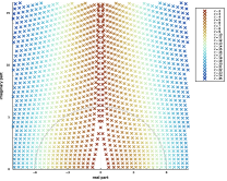
(a) Schwarzschild frequencies

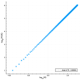
(b) $N(R)$ for Schwarzschild

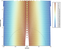
(c) Schw.-dS frequencies frequencies

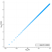
(d) $N(R)$ for Schw.-dS

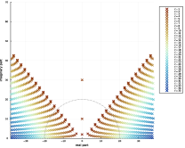
(e) Schw.-AdS frequencies

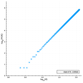
(f) $N(R)$ for Schw.-AdS

Figure 18: . Panels (18a), (18c) and (18e) show the quasinormal frequencies for different quantum numbers $\ell$. Panels (18b), (18d) and (18f) count the number of modes $N(R)$ within a circle of radius $R$ centered at $0+0i$, these panels each have a total of 200 points. The linear fit is performed with a few dozens of points at the end of the series.

In reference [34] a Weyl’s law is conjectured for BH QNM asymptotics. Specifically, given the QNM counting function $N(\omega)$, defined as

$$N(\omega)=\#\{\omega_{n}\in\mathbb{C},\hbox{ such that }|\omega_{n}|\leq\omega\}\ ,$$ (174)

it is conjectured that, for a $(d+1)$-dimensional BH spacetime, $N(\omega)$ satisfies the Weyl’s law

$$N(\omega)\sim\omega^{d}\quad,\quad\omega\to\infty\ ,$$ (175)

independently of the asymptotics. Although (semi-)analytical expressions suggest that this is valid for generic spacetime asymptotics, the fact is that all numerical examples in [34] involve asymptotically flat spacetimes (Schwarzschild and Reissner-Nordström). In Fig. 18 the Weyl’s asymptotics $N(\omega)\sim\omega^{3}$ are numerically recovered for $3+1$-dimensional Schwarzschild, Schwarzschild-de Sitter and Schwarzschild-Anti de Sitter. This is, to our knowledge, the first evidence that the (full) conjecture holds true also in dS and AdS BH asymptotics. The conjecture remains an open-problem, but the numerical evidence here presented strongly supports its universality with respect to spacetime asymptotics.

References

- [1] L. Al Sheikh, Scattering resonances and Pseudospectrum : stability and completeness aspects in optical and gravitational systems, Theses, Université Bourgogne Franche-Comté, Feb. 2022.
- [2] M. Ammon, S. Grieninger, A. Jimenez-Alba, R. P. Macedo, & L. Melgar, Holographic quenches and anomalous transport, JHEP 09, 131 (2016).
- [3] M. Ansorg & R. Panosso Macedo, Spectral decomposition of black-hole perturbations on hyperboloidal slices, Phys. Rev. D93(12), 124016 (2016).
- [4] D. Areán, D. G. Fariña, & K. Landsteiner, Pseudospectra of holographic quasinormal modes, Journal of High Energy Physics 2023(12), 1–60 (2023).
- [5] H. R. Beyer, On the completeness of the quasinormal modes of the Poschl-Teller potential, Commun. Math. Phys. 204, 397–423 (1999).
- [6] W.-J. Beyn, Y. Latushkin, & J. Rottmann-Matthes, Finding eigenvalues of holomorphic Fredholm operator pencils using boundary value problems and contour integrals, arXiv e-prints , arXiv:1210.3952 (Oct. 2012).
- [7] W.-J. Beyn, An integral method for solving nonlinear eigenvalue problems, Linear Algebra and its Applications 436(10), 3839–3863 (2012), Special Issue dedicated to Heinrich Voss’s 65th birthday.
- [8] P. Bizoń, T. Chmaj, & P. Mach, A toy model of hyperboloidal approach to quasinormal modes, Acta Phys. Polon. B 51, 1007 (2020).
- [9] V. Boyanov, V. Cardoso, K. Destounis, J. L. Jaramillo, & R. P. Macedo, Structural aspects of the anti–de Sitter black hole pseudospectrum, Phys. Rev. D 109, 064068 (Mar 2024).
- [10] V. Boyanov, K. Destounis, J. L. Jaramillo, R. P. Macedo, & V. Cardoso, Pseudospectrum of horizonless compact objects: a bootstrap instability mechanism, In preparation (2022).
- [11] J. Carballo & B. Withers, Transient dynamics of quasinormal mode sums, Journal of High Energy Physics 2024(10) (Oct. 2024).
- [12] J.-N. Chen, L.-B. Wu, & Z.-K. Guo, The pseudospectrum and transient of Kaluza–Klein black holes in Einstein–Gauss–Bonnet gravity, Classical and Quantum Gravity 41(23), 235015 (nov 2024).
- [13] E. S. C. Ching, P. T. Leung, A. Maassen van den Brink, W. M. Suen, S. S. Tong, & K. Young, Quasinormal-mode expansion for waves in open systems, Rev. Mod. Phys. 70, 1545–1554 (Oct 1998).
- [14] E. S. C. Ching, P. T. Leung, W. M. Suen, & K. Young, Quasinormal Mode Expansion for Linearized Waves in Gravitational Systems, Phys. Rev. Lett. 74, 4588–4591 (Jun 1995).
- [15] B. Cownden, C. Pantelidou, & M. Zilhão, The pseudospectra of black holes in AdS, Journal of High Energy Physics 2024(5), 1–39 (2024).
- [16] K. Destounis, V. Boyanov, & R. Panosso Macedo, Pseudospectrum of de Sitter black holes, Phys. Rev. D 109(4), 044023 (2024).
- [17] K. Destounis & F. Duque, Black-hole spectroscopy: quasinormal modes, ringdown stability and the pseudospectrum, in Compact Objects in the Universe, pages 155–202, Springer, 2024.
- [18] K. Destounis, R. P. Macedo, E. Berti, V. Cardoso, & J. L. Jaramillo, Pseudospectrum of Reissner-Nordström black holes: Quasinormal mode instability and universality, Phys. Rev. D 104(8), 084091 (2021).
- [19] S. Dyatlov & M. Zworski, Mathematical Theory of Scattering Resonances, Graduate Studies in Mathematics, American Mathematical Society, 2019.
- [20] D. Gajic & C. Warnick, A model problem for quasinormal ringdown of asymptotically flat or extremal black holes, J. Math. Phys. 61(10), 102501 (2020).
- [21] D. Gajic & C. Warnick, Quasinormal Modes in Extremal Reissner–Nordström Spacetimes, Commun. Math. Phys. 385(3), 1395–1498 (2021).
- [22] D. Gajic & C. M. Warnick, Quasinormal modes on Kerr spacetimes, arXiv preprint arXiv:2407.04098 (2024).
- [23] J. Galkowski & M. Zworski, Outgoing solutions via Gevrey-2 properties, Annals of PDE 7, 1–13 (2021).
- [24] G. Gamow, Zur Quantentheorie des Atomkernes, Zeitschrift fur Physik 51(3-4), 204–212 (Mar. 1928).
- [25] E. Gasperin & J. L. Jaramillo, Energy scales and black hole pseudospectra: the structural role of the scalar product, Class. Quant. Grav. 39(11), 115010 (2022).
- [26] S. R. Green, S. Hollands, L. Sberna, V. Toomani, & P. Zimmerman, Conserved currents for a Kerr black hole and orthogonality of quasinormal modes, Phys. Rev. D 107(6), 064030 (2023).
- [27] J. B. Griffiths & J. Podolský, Exact Space-Times in Einstein’s General Relativity, Cambridge Monographs on Mathematical Physics, Cambridge University Press, 2009.
- [28] M. Hitrik & M. Zworski, Overdamped QNM for Schwarzschild black holes, 2024.
- [29] J. Besson et al., Keldysh quasi-normal mode expansions of black hole perturbations: convergence and regularity aspects, in preparation, 2025.
- [30] J. Besson, Piotr Bizoń , J.L. Jaramillo and Daniel Pook-Kolb, Keldysh quasi-normal mode expansions of black hole perturbations: convergence and regularity aspects, in preparation, 2025.
- [31] J. Besson, V. Boyanov, and J. L. Jaramillo, Black hole quasi-normal modes as eigenvalues: definition and stability problem, in preparation, 2025.
- [32] J. L. Jaramillo, Pseudospectrum and binary black hole merger transients, Class. Quant. Grav. 39(21), 217002 (2022).
- [33] J. L. Jaramillo, R. Panosso Macedo, & L. Al Sheikh, Pseudospectrum and Black Hole Quasinormal Mode Instability, Phys. Rev. X 11(3), 031003 (2021).
- [34] J. L. Jaramillo, R. Panosso Macedo, O. Meneses-Rojas, B. Raffaelli, & L. A. Sheikh, A Weyl law for black holes, Phys. Rev. D 110(10), 104008 (2024).
- [35] J. L. Jaramillo, R. Panosso Macedo, & L. A. Sheikh, Gravitational Wave Signatures of Black Hole Quasinormal Mode Instability, Phys. Rev. Lett. 128(21), 211102 (2022).
- [36] J. Joykutty, Existence of Zero-Damped Quasinormal Frequencies for Nearly Extremal Black Holes, Annales Henri Poincare 23(12), 4343–4390 (2022).
- [37] J. Joykutty, Quasinormal Modes of Nearly Extremal Black Holes, PhD thesis, Department of Applied Mathematics And Theoretical Physics, Cambridge U., 2024.
- [38] P. Lalanne, W. Yan, K. Vynck, C. Sauvan, & J.-P. Hugonin, Light Interaction with Photonic and Plasmonic Resonances, Laser & Photonics Review 12(5), 1700113 (May 2018).
- [39] P. Lalanne, W. Yan, K. Vynck, C. Sauvan, & J. Hugonin, Light Interaction with Photonic and Plasmonic Resonances, Laser & Photonics Reviews 12(5), 1700113 (2018).
- [40] P. D. Lax & R. S. Phillips, Scattering theory, volume 26 of Pure and Applied Mathematics, Academic Press, Boston, second edition edition, 1989.
- [41] P. T. Leung, S. Y. Liu, & K. Young, Completeness and orthogonality of quasinormal modes in leaky optical cavities, Phys. Rev. A 49, 3057–3067 (Apr 1994).
- [42] R. P. Macedo & A. Zenginoglu, Hyperboloidal Approach to Quasinormal Modes, arXiv preprint arXiv:2409.11478 (2024).
- [43] A. S. Markus, Introduction to the spectral theory of polynomial operator pencils, American Mathematical Soc., 2012.
- [44] R. B. Melrose, Geometric scattering theory, volume 1, Cambridge University Press, 1995.
- [45] R. Mennicken & M. Möller, Non-Self-Adjoint Boundary Eigenvalue Problems, ISSN, Elsevier Science, 2003.
- [46] N. Moiseyev, Non-Hermitian quantum mechanics, Cambridge University Press, 2011.
- [47] A. Nicolet, G. Demésy, F. Zolla, C. Campos, J. E. Roman, & C. Geuzaine, Physically agnostic quasi normal mode expansion in time dispersive structures: From mechanical vibrations to nanophotonic resonances, European Journal of Mechanics-A/Solids 100, 104809 (2023).
- [48] H.-P. Nollert & R. H. Price, Quantifying excitations of quasinormal mode systems, J. Math. Phys. 40, 980–1010 (1999).
- [49] R. Panosso Macedo, Hyperboloidal framework for the Kerr spacetime, Class. Quant. Grav. 37(6), 065019 (2020).
- [50] R. Panosso Macedo, Hyperboloidal approach for static spherically symmetric spacetimes: a didactical introduction and applications in black-hole physics, Philosophical Transactions of the Royal Society A 382(2267), 20230046 (2024).
- [51] R. Panosso Macedo & M. Ansorg, Axisymmetric fully spectral code for hyperbolic equations, J. Comput. Phys. 276, 357–379 (2014).
- [52] R. Panosso Macedo, J. L. Jaramillo, & M. Ansorg, Hyperboloidal slicing approach to quasi-normal mode expansions: the Reissner-Nordström case, Phys. Rev. D98(12), 124005 (2018).
- [53] R. Panosso Macedo & A. Zenginoglu, Hyperboloidal Approach to Quasinormal Modes, (9 2024).
- [54] S. Sarkar, M. Rahman, & S. Chakraborty, Perturbing the perturbed: Stability of quasinormal modes in presence of a positive cosmological constant, Phys. Rev. D 108, 104002 (Nov 2023).
- [55] P. J. Schmid, Nonmodal Stability Theory, Annual Review of Fluid Mechanics 39(1), 129–162 (2007).
- [56] B. Simon, Resonances and complex scaling: A rigorous overview, International Journal of Quantum Chemistry 14(4), 529–542 (1978).
- [57] S.-H. Tang & M. Zworski, Resonance expansions of scattered waves, Communications on Pure and Applied Mathematics 53(10), 1305–1334 (2000).
- [58] L. N. Trefethen, A. E. Trefethen, S. C. Reddy, & T. A. Driscoll, Hydrodynamic Stability Without Eigenvalues, Science 261(5121), 578–584 (1993).
- [59] L. Trefethen & M. Embree, Spectra and Pseudospectra: The Behavior of Nonnormal Matrices and Operators, Princeton University Press, 2005.
- [60] B. R. Vainberg, Exterior elliptic problems that depend polynomially on the spectral parameter, and the asymptotic behavior for large values of the time of the solutions of nonstationary problems, Mat. Sb. (N.S.) 92(134), 224–241 (1973).
- [61] C. Warnick, (In)completeness of Quasinormal Modes, Acta Phys. Pol. B Proc. Suppl. 15, 1-A13 (2022).
- [62] C. Warnick, (In)stability of de Sitter Quasinormal Mode spectra, 2024.
- [63] C. M. Warnick, On quasinormal modes of asymptotically anti-de Sitter black holes, Commun. Math. Phys. 333(2), 959–1035 (2015).
- [64] S. Yakubov, Completeness of root functions of regular differential operators, volume 71, CRC Press, 1993.
- [65] A. Zenginoglu & et al., Hyperboloidal research network: https://hyperboloid.al/.
- [66] A. Zenginoğlu, Hyperboloidal foliations and scri-fixing, Classical and Quantum Gravity 25(14), 145002 (2008).
- [67] A. Zenginoglu, A Geometric framework for black hole perturbations, Phys. Rev. D83, 127502 (2011).
- [68] A. Zenginoğlu, Hyperbolic times in Minkowski space, arXiv preprint arXiv:2404.01528 (2024).
- [69] M. Zworski, Mathematical study of scattering resonances, Bulletin of Mathematical Sciences 7(1), 1–85 (2017).