Chain-linked Multiple Matrix Integration via Embedding Alignment

Abstract

Motivated by the increasing demand for multi-source data integration in various scientific fields, in this paper we study matrix completion in scenarios where the data exhibits certain block-wise missing structures – specifically, where only a few noisy submatrices representing (overlapping) parts of the full matrix are available. We propose the Chain-linked Multiple Matrix Integration (CMMI) procedure to efficiently combine the information that can be extracted from these individual noisy submatrices. CMMI begins by deriving entity embeddings for each observed submatrix, then aligns these embeddings using overlapping entities between pairs of submatrices, and finally aggregates them to reconstruct the entire matrix of interest. We establish, under mild regularity conditions, entrywise error bounds and normal approximations for the CMMI estimates. Simulation studies and real data applications show that CMMI is computationally efficient and effective in recovering the full matrix, even when overlaps between the observed submatrices are minimal.

Keywords: $2\to\infty$ norm, normal approximations, matrix completion, data integration

1 Introduction

The development of large-scale data collection and sharing has sparked considerable research interests in integrating data from diverse sources to efficiently uncover underlying signals. This problem is especially pertinent in fields such as healthcare research (Hong et al., 2021; Zhou et al., 2023), genomic data integration (Maneck et al., 2011; Tseng et al., 2015; Cai et al., 2016), single-cell data integration (Stuart et al., 2019; Ma et al., 2024), and chemometrics (Mishra et al., 2021). In this paper we consider a formulation of the problem where each source $i$ corresponds to a partially observed submatrix $\mathbf{M}^{(i)}$ of some matrix $\mathbf{M}$, and the goal is to integrate these $\{\mathbf{M}^{(i)}\}$ to recover $\mathbf{M}$ as accurately as possible.

As a first motivating example, consider pointwise mutual information (PMI) constructed from different electronic healthcare records (EHR) datasets. PMI quantities the association between a pair of clinical concepts, and matrices representing these associations can be derived from co-occurrence summaries of various EHR datasets (Ahuja et al., 2020; Zhou et al., 2022). However, due to the lack of interoperability across healthcare systems (Rajkomar et al., 2018), different EHR data often involve non-identical concepts with limited overlap, resulting in substantial differences among their PMI matrices. The analysis of PMI matrices from different EHR datasets can thus be viewed as a multi-source matrix integration problem. Specifically, let $\mathcal{U}$ represent some concept set and suppose there is a symmetric PMI matrix $\mathbf{P}\in\mathbb{R}^{N\times N}$ associated with $\mathcal{U}$, where $N:=|\mathcal{U}|$. For the $i$th EHR, we denote its clinical concept by $\mathcal{U}_{i}\subset\mathcal{U}$ and let $n_{i}:=|\mathcal{U}_{i}|$. The PMI matrix derived from the $i$th EHR, $\mathbf{A}^{(i)}\in\mathbb{R}^{n_{i}\times n_{i}}$, then corresponds to the principal submatrix of $\mathbf{P}$ associated with $\mathcal{U}_{i}$. As it is often the case that the union of all the entries in $\{\mathbf{A}^{(i)}\}$ constitutes only a strict subset of those in $\mathbf{P}$, our aim is to integrate these $\{\mathbf{A}^{(i)}\}$ to recover the unobserved entries in $\mathbf{P}$.

For another example, consider single-cell matrix data where rows represent genomic features, columns represent cells, and each entry records some specific information about a feature in the corresponding cell. A key challenge in the joint analysis for this type of data is to devise efficient computational strategies to integrate different data modalities (Ma et al., 2020; Lähnemann et al., 2020), as the experimental design may lead to a collection of single-cell data matrices for different, but potentially overlapping, sets of cells and features. More specifically, let $\mathbf{P}\in\mathbb{R}^{N\times M}$ be the population matrix for all involved features and cells where $N:=|\mathcal{U}|,M:=|\mathcal{V}|$ (with $\mathcal{U}$ and $\mathcal{V}$ denoting the sets of genomic features and cells, respectively). Each single-cell data matrix $\mathbf{A}^{(i)}\in\mathbb{R}^{n_{i}\times m_{i}}$ is then a submatrix of $\mathbf{P}$ corresponding to some $\mathcal{U}_{i}\subset\mathcal{U}$ and $\mathcal{V}_{i}\subset\mathcal{V}$; here we denote $n_{i}:=|\mathcal{U}_{i}|$ and $m_{i}:=|\mathcal{V}_{i}|$. Our aim is once again to integrate the collection of $\{\mathbf{A}^{(i)}\}$ to reconstruct the original $\mathbf{P}$.

The above examples involving EHR and single-cell data are special cases of the matrix completion with noise and block-wise missing structures. However, the existing literature on matrix completion mainly focuses on recovering a possibly low-rank matrix based on uniformly sampled observed entries or independently sampled observed entries which may be contaminated by noise; see, e.g., Candès and Tao (2010); Candes and Recht (2012); Cai et al. (2010); Candes and Plan (2011); Koltchinskii et al. (2011); Tanner and Wei (2013); Chen et al. (2019); Fornasier et al. (2011); Mohan and Fazel (2012); Lee and Bresler (2010); Vandereycken (2013); Hu et al. (2012); Sun and Luo (2016); Cho et al. (2017); Chen et al. (2020); Yan et al. (2024); Srebro and Salakhutdinov (2010); Foygel et al. (2011); Cai and Zhou (2016); Keshavan et al. (2010) for an incomplete list of references.

These assumptions of uniform or independent sampling in standard matrix completion models are generally violated in applications of matrix integration, thus necessitating the development of efficient methods for tackling the block-wise missing structures. Some examples of this development include the generalized integrative principal component analysis (GIPCA) of Zhu et al. (2020), structured matrix completion (SMC) of Cai et al. (2016), block-wise overlapping noisy matrix integration (BONMI) of Zhou et al. (2023), and symmetric positive semidefinite matrix completion (SPSMC) of Bishop and Yu (2014). The GIPCA procedure operates under the setting where each data matrix have some common samples and completely different variables, and furthermore assumes that each entry in these matrices are from some exponential family of distribution, with entries in the same matrix having the same distributional form. SMC is a spectral procedure for recovering the missing block of an approximately low-rank matrix when a subset of the rows and columns are observed; thus, SMC is designed to impute only a single missing block at a time. BONMI is also a spectral procedure for recovering a missing block (or submatrix) in an approximately low-rank matrix but, in contrast to SMC, assumes that this missing block is associated with a given pair of observed submatrices that share some (limited) overlap. SPSMC has a similar spectral procedure with BONMI to recover a low-rank symmetric positive semidefinite matrix using some observed principal submatrices. While BONMI combines submatrices pair by pair, SPSMC sequentially integrates each new submatrix with the combined structure formed by all previously integrated submatrices. The key idea behind BONMI and SPSMC is to align (via an orthogonal transformation) the spectral embeddings given by the leading (scaled) eigenvectors of the two overlapping submatrices and then impute the missing block by taking the outer product of these aligned embeddings. The use of embedding alignments also appeared in other applications including bilingual dictionary induction (Kementchedjhieva et al., 2018), knowledge graphs integration (Lin et al., 2019; Fanourakis et al., 2023), and vertex nominations (Zheng et al., 2022).

In this paper, we extend the BONMI procedure, which handles only two overlapping submatrices, to $K\geq 2$ submatrices and propose the Chain-linked Multiple Matrix Integration (CMMI) for more efficient and flexible matrix completion. As a motivating example, suppose we have two overlapping pairs of submatrices $(\mathbf{A}^{(1)},\mathbf{A}^{(2)})$ and $(\mathbf{A}^{(2)},\mathbf{A}^{(3)})$. Using the overlapping entries between $\mathbf{A}^{(1)}$ and $\mathbf{A}^{(2)}$ (resp. $\mathbf{A}^{(2)}$ and $\mathbf{A}^{(3)}$) we can find an orthogonal transformation $\mathbf{W}^{(1,2)}$ (resp. $\mathbf{W}^{(2,3)}$) to align the embeddings $\hat{\mathbf{X}}^{(1)}$ and $\hat{\mathbf{X}}^{(2)}$ (resp. $\hat{\mathbf{X}}^{(2)}$ and $\hat{\mathbf{X}}^{(3)}$). Then by combining $\mathbf{W}^{(1,2)}$ and $\mathbf{W}^{(2,3)}$, we can also align $\hat{\mathbf{X}}^{(1)}$ to $\hat{\mathbf{X}}^{(3)}$ and recover the missing block associated with $\mathbf{A}^{(1)}$ and $\mathbf{A}^{(3)}$ even when these submatrices are non-overlapping. Generalizing this observation we can show that as long as $\{\mathbf{A}^{(i)}\}$ are connected then we can integrate them simultaneously to recover all the missing entries; here two submatrices $\mathbf{A}^{(i)}$ and $\mathbf{A}^{(j)}$ are said to be connected if there exists a sequence $i_{0},i_{1},\dots,i_{L}$ with $i_{0}=i$, $i_{L}=j$ such that $\mathbf{A}^{(i_{\ell-1})}$ and $\mathbf{A}^{(i_{\ell})}$ are overlapping for all $\ell=1,\dots,L$. The use of CMMI thus enables the recovery of many missing blocks that are unrecoverable by BONMI and furthermore allows for significantly smaller overlap between the observed submatrices. CMMI considers all possible overlapping pairs without relying on the integration order of submatrices, unlike SPSMC, enabling a more optimal recovery result.

The structure of our paper is as follows. In Section 2 we introduce the model for multiple observed principal submatrices of a whole symmetric positive semi-definite matrix, and propose CMMI to integrate a chain of connected overlapping submatrices. Theoretical results for our CMMI procedures are presented in Section 3. In particular we derive error bounds in two-to-infinity norm for the spectral embedding of the submatrices and entrywise error bound for the recovered entries. Using these error bounds we show that our recovered entries are approximately normally distributed around their true values and that our algorithm yields consistent estimate even when there are only minimal overlap between the submatrices. We emphasize that the results in Section 3 also hold for BONMI (which is a special case of our results for $K=2$) and SPSMC, thereby providing significant refinements over those in Zhou et al. (2023) and Bishop and Yu (2014), which mainly focus on bounding the spectral or Frobenius norm errors of the missing block and embeddings. And our analysis handles both noisy and missing entries in the observed submatrices while Zhou et al. (2023) and Bishop and Yu (2014) only consider the case of noisy entries. Numerical simulations and experiments on real data are presented in Sections 4 and 5. In Section 6, we extend our embedding alignment approach to the cases of symmetric indefinite matrices and asymmetric or rectangular matrices. Detailed proofs of stated results are provided in the supplementary material. Section A in the supplementary material explores more complex matrix integration challenges, such as scenarios where the connected submatrices do not form a single chain but rather multiple chains with possibly quite different lengths and thus we need to select a suitably optimal chain among these candidates. The theoretical results in Section 3 allows us to develop several effective strategies for addressing these issues.

1.1 Notations

We summarize some notations used in this paper. For any positive integer $n$, we denote by $[n]$ the set $\{1,2,\dots,n\}$. For two non-negative sequences $\{a_{n}\}_{n\geq 1}$ and $\{b_{n}\}_{n\geq 1}$, we write $a_{n}\lesssim b_{n}$ (resp. $a_{n}\gtrsim b_{n}$) if there exists some constant $C>0$ such that $a_{n}\leq Cb_{n}$ (resp. $a_{n}\geq Cb_{n}$) for all $n\geq 1$, and we write $a_{n}\asymp b_{n}$ if $a_{n}\lesssim b_{n}$ and $a_{n}\gtrsim b_{n}$. The notation $a_{n}\ll b_{n}$ (resp. $a_{n}\gg b_{n}$) means that there exists some sufficiently small (resp. large) constant $C>0$ such that $a_{n}\leq Cb_{n}$ (resp. $a_{n}\geq Cb_{n}$). If $a_{n}/b_{n}$ stays bounded away from $+\infty$, we write $a_{n}=O(b_{n})$ and $b_{n}=\Omega(a_{n})$, and we use the notation $a_{n}=\Theta(b_{n})$ to indicate that $a_{n}=O(b_{n})$ and $a_{n}=\Omega(b_{n})$. If $a_{n}/b_{n}\to 0$, we write $a_{n}=o(b_{n})$ and $b_{n}=\omega(a_{n})$. We say a sequence of events $\mathcal{A}_{n}$ holds with high probability if for any $c>0$ there exists a finite constant $n_{0}$ depending only on $c$ such that $\mathbb{P}(\mathcal{A}_{n})\geq 1-n^{-c}$ for all $n\geq n_{0}$. We write $a_{n}=O_{p}(b_{n})$ (resp. $a_{n}=o_{p}(b_{n})$) to denote that $a_{n}=O(b_{n})$ (resp. $a_{n}=o(b_{n})$) holds with high probability. We denote by $\mathcal{O}_{d}$ the set of $d\times d$ orthogonal matrices. For any matrix $\mathbf{M}\in\mathbb{R}^{A\times B}$ and index sets $\mathcal{A}\subseteq[A]$, $\mathcal{B}\subseteq[B]$, we denote by $\mathbf{M}_{\mathcal{A},\mathcal{B}}\in\mathbb{R}^{|\mathcal{A}|\times|\mathcal{B}|}$ the submatrix of $\mathbf{M}$ formed from rows $\mathcal{A}$ and columns $\mathcal{B}$, and we denote by $\mathbf{M}_{\mathcal{A}}\in\mathbb{R}^{|\mathcal{A}|\times B}$ the submatrix of $\mathbf{M}$ consisting of the rows indexed by $\mathcal{A}$. The Hadamard or entrywise product between two conformal matrices $\mathbf{M}$ and $\mathbf{N}$ is denoted by $\mathbf{M}\circ\mathbf{N}$. Given a matrix $\mathbf{M}$, we denote its spectral, Frobenius, and infinity norms by $\|\mathbf{M}\|$, $\|\mathbf{M}\|_{F}$, and $\|\mathbf{M}\|_{\infty}$, respectively. We also denote the maximum entry (in modulus) of $\mathbf{M}$ by $\|\mathbf{M}\|_{\max}$ and the $2\to\infty$ norm of $\mathbf{M}$ by

$$\|\mathbf{M}\|_{2\to\infty}=\max_{\|\bm{x}\|=1}\|\mathbf{M}\bm{x}\|_{\infty}=\max_{i}\|\mathbf{m}_{i}\|,$$

where $\mathbf{m}_{i}$ denotes the $i$th row of $\mathbf{M}$, i.e., $\|\mathbf{M}\|_{2\to\infty}$ is the maximum of the $\ell_{2}$ norms of the rows of $\mathbf{M}$. We note that the $2\to\infty$ norm is not sub-multiplicative. However, for any matrices $\mathbf{M}$ and $\mathbf{N}$ of conformal dimensions, we have

$$\|\mathbf{M}\mathbf{N}\|_{2\to\infty}\leq\min\{\|\mathbf{M}\|_{2\to\infty}\times\|\mathbf{N}\|,\|\mathbf{M}\|_{\infty}\times\|\mathbf{N}\|_{2\to\infty}\};$$

see Proposition 6.5 in Cape et al. (2019). Perturbation bounds using the $2\to\infty$ norm for the eigenvectors and/or singular vectors of a noisily observed matrix had recently attracted interests from the statistics community, see e.g., Chen et al. (2021); Cape et al. (2019); Fan et al. (2018); Abbe et al. (2020) and the references therein.

2 Methodology

We are interested in an unobserved population matrix associated with $N$ entities denoted by $\mathbf{P}\in\mathbb{R}^{N\times N}$. We assume $\mathbf{P}$ is positive semi-definite with rank $d\ll N$; extensions to the case of symmetric but indefinite $\mathbf{P}$ as well as asymmetric or rectangular $\mathbf{P}$ are discussed in Section 6. Denote the eigen-decomposition of $\mathbf{P}$ as $\mathbf{U}\bm{\Lambda}\mathbf{U}^{\top}$, where $\bm{\Lambda}\in\mathbb{R}^{d\times d}$ is a diagonal matrix whose diagonal entries are the non-zero eigenvalues of $\mathbf{P}$ in descending order, and the orthonormal columns of $\mathbf{U}\in\mathbb{R}^{N\times d}$ constitute the corresponding eigenvectors. The latent positions associated to the entities are given by $\mathbf{X}=\mathbf{U}\bm{\Lambda}^{1/2}\in\mathbb{R}^{N\times d}$ and any entry in $\mathbf{P}$ can be written as the inner product of these latent positions, i.e., $\mathbf{P}=\mathbf{X}\mathbf{X}^{\top}$ so that $\mathbf{P}_{s,t}=\mathbf{x}_{s}^{\top}\mathbf{x}_{t}$ for any $s,t\in[N]$, where $\mathbf{x}_{s}$ and $\mathbf{x}_{t}$ denote the $s$th and $t$th row of $\mathbf{X}$, respectively.

We assume that the entries of $\mathbf{P}$ are only partially observed, and furthermore, that the observed entries can be grouped into blocks. More specifically, suppose that we have $K$ sources and for any $i\in[K]$ we denote the index set of the entities contained in the $i$th source by $\mathcal{U}_{i}\subseteq[N]$. For ease of exposition we also require $\mathcal{U}_{i}\cap(\cup_{j\not=i}\mathcal{U}_{j})\not=\varnothing$ for all $i\in[K]$ as otherwise there exists some $i_{*}$ such that it is impossible to integrate observations from $\mathcal{U}_{i_{*}}$ with those from $\{\mathcal{U}_{j}\}_{j\not=i_{*}}$. We denote $n_{i}:=|\mathcal{U}_{i}|$ and the population matrix for the $i$th source by $\mathbf{P}^{(i)}\in\mathbb{R}^{n_{i}\times n_{i}}$. We then have

$$\mathbf{P}^{(i)}=\mathbf{P}_{\mathcal{U}_{i},\mathcal{U}_{i}}=\mathbf{U}_{\mathcal{U}_{i}}\bm{\Lambda}\mathbf{U}_{\mathcal{U}_{i}}^{\top}=\mathbf{X}_{\mathcal{U}_{i}}\mathbf{X}_{\mathcal{U}_{i}}^{\top},$$

where $\mathbf{P}_{\mathcal{U}_{i},\mathcal{U}_{i}}$ is the submatrix of $\mathbf{P}$ formed from rows and columns in $\mathcal{U}_{i}$, $\mathbf{U}_{\mathcal{U}_{i}}\in\mathbb{R}^{n_{i}\times d}$ contains the rows of $\mathbf{U}$ in $\mathcal{U}_{i}$, and $\mathbf{X}_{\mathcal{U}_{i}}\in\mathbb{R}^{n_{i}\times d}$ contains the latent positions of $\mathcal{U}_{i}$.

We also allow for missing and corrupted observations in each source, i.e., for the $i$th source we only get to observe $\mathbf{P}^{(i)}_{s,t}+\mathbf{N}^{(i)}_{s,t}$ for all $\mathbf{\Omega}^{(i)}_{s,t}=1.$ Here $\mathbf{\Omega}^{(i)}\in\{0,1\}^{n_{i}\times n_{i}}$ indicates the indices of the observed entries and $\mathbf{N}^{(i)}\in\mathbb{R}^{n_{i}\times n_{i}}$ represent the random noise. In particular $\mathbf{\Omega}^{(i)}$ and $\mathbf{N}^{(i)}$ are both symmetric, and we assume the upper triangular entries of $\mathbf{\Omega}^{(i)}$ are i.i.d. Bernoulli random variables with success probability $q_{i}$ while the upper triangular entries of $\mathbf{N}^{(i)}$ are independent, mean-zero sub-Gaussian random variables with Orlicz-2 norm bounded by $\sigma_{i}=\max_{s,t\in[n_{i}]}\|\mathbf{N}^{(i)}_{s,t}\|_{\psi_{2}}$. For this model, the matrix

$$\mathbf{A}^{(i)}=(\mathbf{P}^{(i)}+\mathbf{N}^{(i)})\circ\mathbf{\Omega}^{(i)}/q_{i}$$ (2.1)

is an unbiased estimate of $\mathbf{P}^{(i)}$, and thus a natural idea is to use the scaled leading eigenvectors $\hat{\mathbf{X}}^{(i)}=\hat{\mathbf{U}}^{(i)}(\hat{\bm{\Lambda}}^{(i)})^{1/2}$ as an estimate for $\mathbf{X}_{\mathcal{U}_{i}}$, where $\hat{\bm{\Lambda}}^{(i)}$ and $\hat{\mathbf{U}}^{(i)}$ contain the leading eigenvalues and the leading eigenvectors of $\mathbf{A}^{(i)}$, respectively. We now propose an algorithm to integrate and align $\{\hat{\mathbf{X}}^{(i)}\}_{i\in[K]}$ for recovery of the unobserved entries in $\mathbf{P}$.

2.1 Motivation of the algorithm

We first summarize the BONMI algorithm of Zhou et al. (2023). We start with the noiseless case for overlapping submatrices $\mathbf{P}^{(1)}$ and $\mathbf{P}^{(2)}$ to illustrate the main ideas. Our goal is to recover the unobserved entries in the white block of Figure 1; this is part of $\mathbf{P}_{\mathcal{U}_{1},\mathcal{U}_{2}}$.

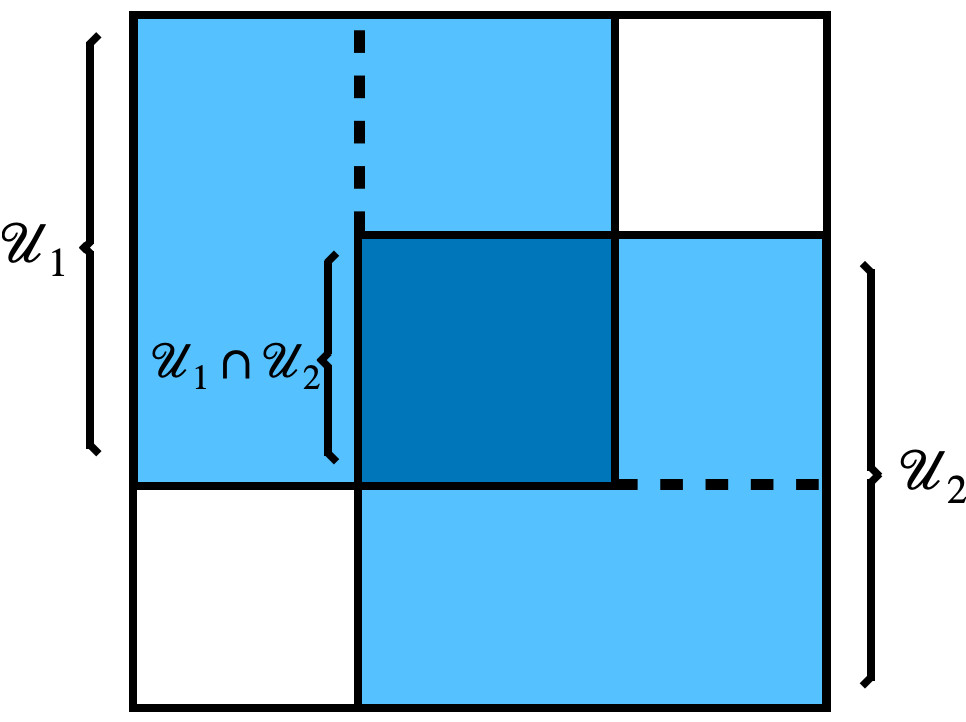
Figure 1: A pair of overlapping observed submatrices

Based on $\mathbf{P}^{(1)}$ and $\mathbf{P}^{(2)}$ we can obtain latent position estimates for entities in $\mathcal{U}_{1}$ and $\mathcal{U}_{2}$, which we denote as $\mathbf{X}^{(1)}$ and $\mathbf{X}^{(2)}$. Next note that

$$\mathbf{X}_{\mathcal{U}_{1}}\mathbf{X}_{\mathcal{U}_{1}}^{\top}=\mathbf{P}_{\mathcal{U}_{1},\mathcal{U}_{1}}=\mathbf{P}^{(1)}=\mathbf{X}^{(1)}\mathbf{X}^{(1)\top},\quad\mathbf{X}_{\mathcal{U}_{2}}\mathbf{X}_{\mathcal{U}_{2}}^{\top}=\mathbf{P}_{\mathcal{U}_{2},\mathcal{U}_{2}}=\mathbf{P}^{(2)}=\mathbf{X}^{(2)}\mathbf{X}^{(2)\top},$$

and hence there exists $\mathbf{W}^{(1)},\mathbf{W}^{(2)}\in\mathcal{O}_{d}$ such that

$$\mathbf{X}_{\mathcal{U}_{1}}=\mathbf{X}^{(1)}\mathbf{W}^{(1)},\quad\mathbf{X}_{\mathcal{U}_{2}}=\mathbf{X}^{(2)}\mathbf{W}^{(2)}.$$ (2.2)

Eq. (2.2) then implies

$$\mathbf{P}_{\mathcal{U}_{1},\mathcal{U}_{2}}=\mathbf{X}_{\mathcal{U}_{1}}\mathbf{X}_{\mathcal{U}_{2}}^{\top}=\mathbf{X}^{(1)}\mathbf{W}^{(1)}\mathbf{W}^{(2)\top}\mathbf{X}^{(2)\top}=\mathbf{X}^{(1)}\mathbf{W}^{(1,2)}\mathbf{X}^{(2)\top},$$ (2.3)

where $\mathbf{W}^{(1,2)}:=\mathbf{W}^{(1)}\mathbf{W}^{(2)\top}\in\mathcal{O}_{d}$, and thus we only need $\mathbf{W}^{(1,2)}$ to recover $\mathbf{P}_{\mathcal{U}_{1},\mathcal{U}_{2}}$.

Note that for entities in $\mathcal{U}_{1}\cap\mathcal{U}_{2}$, we have two equivalent representations of their latent positions. More specifically, let $\mathbf{X}^{(1)}_{\langle\mathcal{U}_{1}\cap\mathcal{U}_{2}\rangle}$ and $\mathbf{X}^{(2)}_{\langle\mathcal{U}_{1}\cap\mathcal{U}_{2}\rangle}$ be the rows of $\mathbf{X}^{(1)}$ and $\mathbf{X}^{(2)}$ corresponding to entities in $\mathcal{U}_{1}\cap\mathcal{U}_{2}$. Then by Eq. (2.2) we have $\mathbf{X}^{(2)}_{\langle\mathcal{U}_{1}\cap\mathcal{U}_{2}\rangle}=\mathbf{X}^{(1)}_{\langle\mathcal{U}_{1}\cap\mathcal{U}_{2}\rangle}\mathbf{W}^{(1,2)}$ and thus $\mathbf{W}^{(1,2)}$ can be obtained by aligning $\mathbf{X}^{(1)}_{\langle\mathcal{U}_{1}\cap\mathcal{U}_{2}\rangle}$ and $\mathbf{X}^{(2)}_{\langle\mathcal{U}_{1}\cap\mathcal{U}_{2}\rangle}$. The resulting $\mathbf{W}^{(1,2)}$ is unique whenever $\mathrm{rk}(\mathbf{P}_{\mathcal{U}_{1}\cap\mathcal{U}_{2},\mathcal{U}_{1}\cap\mathcal{U}_{2}})=d$.

The same approach also extends to the case where the $\mathbf{P}^{(1)}$ and $\mathbf{P}^{(2)}$ are partially and noisily observed. More specifically, suppose we observe $\mathbf{A}^{(1)}$ and $\mathbf{A}^{(2)}$ as defined in Eq. (2.1). We then obtain estimated latent positions $\hat{\mathbf{X}}^{(1)}$ for $\mathcal{U}_{1}$ and $\hat{\mathbf{X}}^{(2)}$ for $\mathcal{U}_{2}$ from $\mathbf{A}^{(1)}$ and $\mathbf{A}^{(2)}$, respectively. To align $\hat{\mathbf{X}}^{(1)}$ and $\hat{\mathbf{X}}^{(2)}$, we solve the orthogonal Procrustes problem

$$\mathbf{W}^{(1,2)}=\underset{\mathbf{O}\in\mathcal{O}_{d}}{\operatorname{argmin}}\|\hat{\mathbf{X}}^{(1)}_{\langle\mathcal{U}_{1}\cap\mathcal{U}_{2}\rangle}\mathbf{O}-\hat{\mathbf{X}}^{(2)}_{\langle\mathcal{U}_{1}\cap\mathcal{U}_{2}\rangle}\|_{F}$$

and then estimate the unobserved block as part of $\hat{\mathbf{P}}_{\mathcal{U}_{1},\mathcal{U}_{2}}=\hat{\mathbf{X}}^{(1)}\mathbf{W}^{(1,2)}\hat{\mathbf{X}}^{(2)\top}.$

2.2 Chain-linked Multiple Matrix Integration (CMMI)

We now extend the ideas in Section 2.1 to a chain of overlapping submatrices. Suppose our goal is to recover the entries in the yellow block of Figure 2, given a collection $\{\mathbf{A}^{(i)}\}_{0\leq i\leq L}$ such that $\mathcal{U}_{i-1}\cap\mathcal{U}_{i}\not=\varnothing$ for all $1\leq i\leq L$. Then for each pair $(\mathcal{U}_{i-1},\mathcal{U}_{i})$, we align the estimated latent position matrices $\hat{\mathbf{X}}^{(i-1)}$ and $\hat{\mathbf{X}}^{(i)}$ by solving the orthogonal Procrustes problem

$$\mathbf{W}^{(i-1,i)}=\underset{\mathbf{O}\in\mathcal{O}_{d}}{\operatorname{argmin}}\|\hat{\mathbf{X}}^{(i-1)}_{\langle\mathcal{U}_{i-1}\cap\mathcal{U}_{i}\rangle}\mathbf{O}-\hat{\mathbf{X}}^{(i)}_{\langle\mathcal{U}_{i-1}\cap\mathcal{U}_{i}\rangle}\|_{F}.$$

Note that the solution of the orthogonal Procrustes problem between matrices $\hat{\mathbf{X}}^{(i-1)}_{\langle\mathcal{U}_{i-1}\cap\mathcal{U}_{i}\rangle}$ and $\hat{\mathbf{X}}^{(i)}_{\langle\mathcal{U}_{i-1}\cap\mathcal{U}_{i}\rangle}$ is given by $\mathbf{W}_{1}\mathbf{W}_{2}^{\top}$ where $\mathbf{W}_{1}$ and $\mathbf{W}_{2}$ contain the left and right singular vectors of $\hat{\mathbf{X}}^{(i-1)\top}_{\langle\mathcal{U}_{i-1}\cap\mathcal{U}_{i}\rangle}\hat{\mathbf{X}}^{(i)}_{\langle\mathcal{U}_{i-1}\cap\mathcal{U}_{i}\rangle}$, respecitvely; see Schönenmann (1966). $\hat{\mathbf{X}}^{(0)}$ and $\hat{\mathbf{X}}^{(L)}$ can be aligned by combining these $\{\mathbf{W}^{(i-1,i)}\}_{1\leq i\leq L}$ which then yields

$$\hat{\mathbf{P}}_{\mathcal{U}_{0},\mathcal{U}_{L}}=\hat{\mathbf{X}}^{(0)}\mathbf{W}^{(0,1)}\mathbf{W}^{(1,2)}\cdots\mathbf{W}^{(L-1,L)}\hat{\mathbf{X}}^{(L)\top}$$

as an estimate for $\mathbf{P}_{\mathcal{U}_{0},\mathcal{U}_{L}}$. See Algorithm 1 for more details.

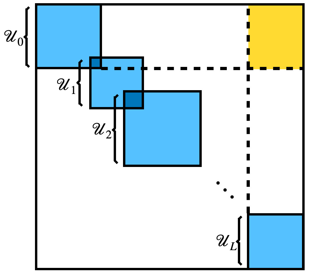
Figure 2: A chain of overlapping observed submatrices

0: Embedding dimension $d$, a chain of overlapping submatrices $\mathbf{A}^{(i_{0})},\mathbf{A}^{(i_{1})},\dots,\mathbf{A}^{(i_{L})}$ for $\mathcal{U}_{i_{0}},\mathcal{U}_{i_{1}},\dots,\mathcal{U}_{i_{L}}$ with $\min\{|\mathcal{U}_{i_{0}}\cap\mathcal{U}_{i_{1}}|,|\mathcal{U}_{i_{1}}\cap\mathcal{U}_{i_{2}}|,\dots,|\mathcal{U}_{i_{L-1}}\cap\mathcal{U}_{i_{L}}|\}\geq d$.

1. For $0\leq\ell\leq L$, obtain estimated latent position matrix for $\mathcal{U}_{i_{\ell}}$, denoted by $\hat{\mathbf{X}}^{(i_{\ell})}=\hat{\mathbf{U}}^{(i_{\ell})}(\hat{\bm{\Lambda}}^{(i_{\ell})})^{1/2}$, where $\hat{\mathbf{U}}^{(i_{\ell})}\in\mathbb{R}^{|\mathcal{U}_{i_{\ell}}|\times d}$ and the diagonal matrix $\hat{\bm{\Lambda}}^{(i_{\ell})}\in\mathbb{R}^{d\times d}$ contain the $d$ leading eigenvectors and eigenvalues of $\mathbf{A}^{(i_{\ell})}$, respectively.

2. For $1\leq\ell\leq L$, obtain $\mathbf{W}^{(i_{\ell-1},i_{\ell})}$ by solving the orthogonal Procrustes problem

   $$\mathbf{W}^{(i_{\ell-1},i_{\ell})}=\underset{\mathbf{O}\in\mathcal{O}_{d}}{\operatorname{argmin}}\|\hat{\mathbf{X}}^{(i_{\ell-1})}_{\langle\mathcal{U}_{i_{\ell-1}}\cap\mathcal{U}_{i_{\ell}}\rangle}\mathbf{O}-\hat{\mathbf{X}}^{(i_{\ell})}_{\langle\mathcal{U}_{i_{\ell-1}}\cap\mathcal{U}_{i_{\ell}}\rangle}\|_{F}.$$

3. Compute $\hat{\mathbf{P}}_{\mathcal{U}_{i_{0}},\mathcal{U}_{i_{L}}}=\hat{\mathbf{X}}^{(i_{0})}\mathbf{W}^{(i_{0},i_{1})}\mathbf{W}^{(i_{1},i_{2})}\cdots\mathbf{W}^{(i_{L-1},i_{L})}\hat{\mathbf{X}}^{(i_{L})\top}$.

0: $\hat{\mathbf{P}}_{\mathcal{U}_{i_{0}},\mathcal{U}_{i_{L}}}$.

Algorithm 1 Chain-linked Multiple Matrix Integration (CMMI) algorithm

Compared to BONMI in Zhou et al. (2023), which handles only two submatrices, our proposed CMMI can combine all connected submatrices, where two submatrices $\mathbf{P}^{(i)}$ and $\mathbf{P}^{(j)}$ are said to be connected if there exists a path of overlapping submatrices between them. Indeed, for the example in Figure 2, BONMI can only recover the entries associated with pairs of overlapping submatrices, namely $\mathbf{P}_{\mathcal{U}_{0},\mathcal{U}_{1}},\mathbf{P}_{\mathcal{U}_{1},\mathcal{U}_{2}},\dots,\mathbf{P}_{\mathcal{U}_{L-1},\mathcal{U}_{L}}$, while CMMI can recover the whole matrix $\mathbf{P}$. In general, BONMI only recovers $O(1/L)$ fraction of the entries recoverable by CMMI. Moreover, our theoretical results indicate that increasing $L$ has a minimal effect on the estimation error of CMMI (see Theorem 2), and simulations and real data experiments in Sections 4 and 5 show that accurate recovery is possible even when $L=20$. Our theoretical results also show that CMMI requires only minimal overlap between $\mathcal{U}_{i-1}$ and $\mathcal{U}_{i}$, e.g., $|\mathcal{U}_{i-1}\cap\mathcal{U}_{i}|$ can be as small as $d$, the embedding dimension of $\{\hat{\mathbf{X}}^{(i)}\}$; see Remark 6 and Section 4.3 for further discussion and experimental results.

For more general cases encountered in practice, there may exist multiple chains to recover a given unobserved entry. We will present in Section A of the supplementary material several strategies to select and/or combine these chains. Although in certain cases, such as when considering a simple chain, CMMI is identical to the sequential integration approach SPSMC in Bishop and Yu (2014), CMMI offers a more optimal strategy in more complex scenarios by considering all overlapping pairs. In contrast, the restriction to sequential integration imposes limitations on SPSMC, and how to determine a valid and effective sequential integration order is an unresolved issue in Bishop and Yu (2014). Furthermore, our theoretical results are significantly stronger than those in Bishop and Yu (2014) and Zhou et al. (2023); see Section 3.1 for further discussion.

3 Theoretical Results

We now present theoretical guarantees for the estimate $\hat{\mathbf{P}}_{\mathcal{U}_{i_{0}},\mathcal{U}_{i_{L}}}$ obtained by Algorithm 1. We shall make the following assumptions on the underlying population matrices $\{\mathbf{P}_{\mathcal{U}_{i},\mathcal{U}_{i}}\}$ for the observed blocks. We emphasize that, because our results address either large-sample approximations or limiting distributions, these assumptions should be interpreted in the regime where $n_{i}$ is arbitrarily large and/or $n_{i}\to\infty$.

Assumption 1.

For each $i$, the following conditions hold for sufficiently large $n_{i}$.

• We have $\mathrm{rk}(\mathbf{P}_{\mathcal{U}_{i},\mathcal{U}_{i}})=d$. Let $\lambda_{i,\max}$ and $\lambda_{i,\min}$ denote the largest and smallest non-zero eigenvalues of $\mathbf{P}_{\mathcal{U}_{i},\mathcal{U}_{i}}$, and let $\mathbf{U}^{(i)}\in\mathbb{R}^{n_{i}\times d}$ contain the eigenvectors corresponding to all non-zero eigenvalues. We then assume

  $$\|\mathbf{U}^{(i)}\|\lesssim\frac{d^{1/2}}{n_{i}^{1/2}},\quad\text{and}\quad\frac{\lambda_{i,\max}}{\lambda_{i,\min}}\leq M$$ (3.1)

  for some finite constant $M>0$.

• $\mathbf{A}^{(i)}=(\mathbf{P}_{\mathcal{U}_{i},\mathcal{U}_{i}}+\mathbf{N}^{(i)})\circ\bm{\Omega}^{(i)}$ where $\mathbf{N}^{(i)}$ is a symmetric matrix whose (upper triangular) entries are independent mean-zero sub-Gaussian random variables with Orlicz-2 norm bounded by $\sigma_{i}$ and $\bm{\Omega}^{(i)}$ is a symmetric binary matrix whose (upper triangular) entries are i.i.d. Bernoulli random variables with success probability $q_{i}$.

• Denote

  $$\mu_{i}:=\lambda_{i,\min}/n_{i},\quad\gamma_{i}:=(\|\mathbf{P}_{\mathcal{U}_{i},\mathcal{U}_{i}}\|_{\max}+\sigma_{i})\log^{1/2}{n_{i}}.$$

  We suppose $q_{i}n_{i}\gtrsim\log^{2}{n_{i}}$ and

  $$\frac{\gamma_{i}}{(q_{i}n_{i})^{1/2}\mu_{i}}\ll 1,\quad\frac{\gamma_{i}}{(q_{i}n_{i}\mu_{i})^{1/2}}\lesssim\|\mathbf{X}_{\mathcal{U}_{i}}\|_{2\to\infty}.$$ (3.2)

Remark 1.

For the entire population matrix $\mathbf{P}\in\mathbb{R}^{N\times N}$, we have $\mathrm{rk}(\mathbf{P})=d$. Let $\lambda_{\max}$ and $\lambda_{\min}$ denote the largest and smallest non-zero eigenvalues of $\mathbf{P}$, and let $\mathbf{U}\in\mathbb{R}^{N\times d}$ contain the eigenvectors corresponding to non-zero eigenvalues. Suppose (1) $\mathbf{P}$ has bounded condition number, i.e., $\lambda_{\max}/\lambda_{\min}\leq M^{\prime}$ for some constant $M^{\prime}>0$, and $\mathbf{U}$ has bounded coherence, i.e., $\|\mathbf{U}\|_{2\to\infty}\lesssim d^{1/2}N^{-1/2}$; (2) for each $i$, $\mathcal{U}_{i}$ are drawn uniformly at random from $\mathcal{U}$. Then

$$\frac{n_{i}}{N}\lambda_{\min}\lesssim\lambda_{i,\min}\leq\lambda_{i,\max}\lesssim\frac{dn_{i}}{N}\lambda_{\max},\quad\text{and}\quad\|\mathbf{U}^{(i)}\|_{2\to\infty}\lesssim\frac{d^{1/2}}{n_{i}^{1/2}}$$ (3.3)

with high probability (Lemma D.11) and Eq. (3.1) holds.

We first consider the case where we only have two overlapping submatrices $\mathbf{A}^{(i)}$ and $\mathbf{A}^{(j)}$. Theorem 1 presents an expansion for $\hat{\mathbf{P}}_{\mathcal{U}_{i_{0}},\mathcal{U}_{i_{L}}}-\mathbf{P}_{\mathcal{U}_{i},\mathcal{U}_{j}}=\hat{\mathbf{X}}^{(i)}\mathbf{W}^{(i,j)}\hat{\mathbf{X}}^{(j)\top}-\mathbf{X}_{\mathcal{U}_{i}}\mathbf{X}_{\mathcal{U}_{j}}^{\top}$.

Theorem 1.

Let $\mathbf{A}^{(i)}$ and $\mathbf{A}^{(j)}$ be overlapping submatrices satisfying Assumption 1. For their overlap, suppose $\mathrm{rk}(\mathbf{P}_{\mathcal{U}_{i}\cap\mathcal{U}_{j},\mathcal{U}_{i}\cap\mathcal{U}_{j}})=d$, and define

$$n_{i,j}:= |\mathcal{U}_{i}\cap\mathcal{U}_{j}|,\quad\vartheta_{i,j}:=\lambda_{\max}(\mathbf{X}_{\mathcal{U}_{i}\cap\mathcal{U}_{j}}^{\top}\mathbf{X}_{\mathcal{U}_{i}\cap\mathcal{U}_{j}}),\quad\theta_{i,j}:=\lambda_{\min}(\mathbf{X}_{\mathcal{U}_{i}\cap\mathcal{U}_{j}}^{\top}\mathbf{X}_{\mathcal{U}_{i}\cap\mathcal{U}_{j}}),$$ (3.4)

$$\alpha_{i,j}:= \frac{n_{i,j}\gamma_{i}\gamma_{j}}{{\theta_{i,j}}(q_{i}n_{i}\mu_{i})^{1/2}(q_{j}n_{j}\mu_{j})^{1/2}}+\frac{{(n_{i,j}\vartheta_{i,j})^{1/2}}}{{\theta_{i,j}}}\Big{(}\frac{\gamma_{i}^{2}}{q_{i}n_{i}\mu_{i}^{3/2}}+\frac{\gamma_{j}^{2}}{q_{j}n_{j}\mu_{j}^{3/2}}\Big{)}$$

$$+\frac{n_{i,j}^{1/2}\|\mathbf{X}_{\mathcal{U}_{i}\cap\mathcal{U}_{j}}\|_{2\to\infty}}{{\theta_{i,j}}}\Big{(}\frac{\gamma_{i}}{(q_{i}n_{i}\mu_{i})^{1/2}}+\frac{\gamma_{j}}{(q_{j}n_{j}\mu_{j})^{1/2}}\Big{)}.$$

Let $\mathbf{E}^{(i)}:=\mathbf{A}^{(i)}-\mathbf{P}^{(i)}$ for any $i$. We then have

$$\hat{\mathbf{P}}_{\mathcal{U}_{i},\mathcal{U}_{j}}-\mathbf{P}_{\mathcal{U}_{i},\mathcal{U}_{j}} =\mathbf{E}^{(i)}\mathbf{X}_{\mathcal{U}_{i}}(\mathbf{X}_{\mathcal{U}_{i}}^{\top}\mathbf{X}_{\mathcal{U}_{i}})^{-1}\mathbf{X}_{\mathcal{U}_{j}}^{\top}+\mathbf{X}_{\mathcal{U}_{i}}(\mathbf{X}_{\mathcal{U}_{j}}^{\top}\mathbf{X}_{\mathcal{U}_{j}})^{-1}\mathbf{X}_{\mathcal{U}_{j}}^{\top}\mathbf{E}^{(j)}+\mathbf{R}^{(i,j)}+\mathbf{S}^{(i,j)},$$ (3.5)

where $\mathbf{R}^{(i,j)}$ and $\mathbf{S}^{(i,j)}$ are random matrices satisfying

$$\|\mathbf{R}^{(i,j)}\|_{\max}\lesssim \frac{\gamma_{i}\gamma_{j}}{(q_{i}n_{i}\mu_{i})^{1/2}(q_{j}n_{j}\mu_{j})^{1/2}}+\Big{(}\frac{\gamma_{i}^{2}}{q_{i}n_{i}\mu_{i}^{3/2}}+\frac{\gamma_{i}}{q_{i}^{1/2}n_{i}\mu_{i}^{1/2}}\Big{)}\|\mathbf{X}_{\mathcal{U}_{j}}\|_{2\to\infty}$$ (3.6)

$$+\Big{(}\frac{\gamma_{j}^{2}}{q_{j}n_{j}\mu_{j}^{3/2}}+\frac{\gamma_{j}}{q_{j}^{1/2}n_{j}\mu_{j}^{1/2}}\Big{)}\|\mathbf{X}_{\mathcal{U}_{i}}\|_{2\to\infty},$$

$$\|\mathbf{S}^{(i,j)}\|_{\max} \lesssim{\alpha_{i,j}}\|\mathbf{X}_{\mathcal{U}_{i}}\|_{2\to\infty}\|\mathbf{X}_{\mathcal{U}_{j}}\|_{2\to\infty}$$ (3.7)

with high probability. Furthermore suppose

$$\alpha_{i,j}\min\Big{\{}\frac{(q_{i}n_{i}\mu_{i})^{1/2}}{\gamma_{i}}\|\mathbf{X}_{\mathcal{U}_{i}}\|_{2\to\infty},\frac{(q_{j}n_{j}\mu_{j})^{1/2}}{\gamma_{j}}\|\mathbf{X}_{\mathcal{U}_{j}}\|_{2\to\infty}\Big{\}}\lesssim 1.$$

Then $\mathbf{E}^{({i})}\mathbf{X}_{\mathcal{U}_{i}}(\mathbf{X}_{\mathcal{U}_{i}}^{\top}\mathbf{X}_{\mathcal{U}_{i}})^{-1}\mathbf{X}_{\mathcal{U}_{j}}^{\top}+\mathbf{X}_{\mathcal{U}_{i}}(\mathbf{X}_{\mathcal{U}_{j}}^{\top}\mathbf{X}_{\mathcal{U}_{j}})^{-1}\mathbf{X}_{\mathcal{U}_{j}}^{\top}\mathbf{E}^{({j})}$ is the dominant term and

$$\|\hat{\mathbf{P}}_{\mathcal{U}_{i},\mathcal{U}_{j}}-\mathbf{P}_{\mathcal{U}_{i},\mathcal{U}_{j}}\|_{\max}\lesssim\frac{\gamma_{i}}{(q_{i}n_{i}\mu_{i})^{1/2}}\|\mathbf{X}_{\mathcal{U}_{j}}\|_{2\to\infty}+\frac{\gamma_{j}}{(q_{j}n_{j}\mu_{j})^{1/2}}\|\mathbf{X}_{\mathcal{U}_{i}}\|_{2\to\infty}$$

with high probability.

Remark 2.

The expansion in Eq. (3.5) consists of four terms, with the first two terms being linear transformations of the additive noise matrices $\mathbf{E}^{(i)}$ and $\mathbf{E}^{(j)}$. The third term $\mathbf{R}^{(i,j)}$ corresponds to second-order estimation errors for $\hat{\mathbf{X}}^{(i)}$ and $\hat{\mathbf{X}}^{(j)}$, and hence Eq. (3.6) only depends on quantities associated with ${\mathbf{X}}_{\mathcal{U}_{i}}$ and ${\mathbf{X}}_{\mathcal{U}_{j}}$. Finally $\mathbf{S}^{(i,j)}$ corresponds to the error when aligning the overlaps $\hat{\mathbf{X}}_{\langle\mathcal{U}_{i}\cap\mathcal{U}_{j}\rangle}^{(i)}$ and $\hat{\mathbf{X}}_{\langle\mathcal{U}_{i}\cap\mathcal{U}_{j}\rangle}^{(j)}$ and hence Eq. (3.7) depends on $\mathbf{X}_{\mathcal{U}_{i}\cap\mathcal{U}_{j}}$.

Remark 3.

Zhou et al. (2023) requires $(n_{i,j}/n_{i})\asymp(n_{i}/N)$ so that the number of overlapping entities must grow with the sizes of the submatrices. However, our derivations of Theorem 1 show that the overlap can be bounded or even be as small as $d$ (the rank of $\mathbf{P}$), which is the minimum value required to align the embeddings in $\mathbb{R}^{d}$; see Remark 6 and Section 4.3 for more detailed discussion and simulations verifying this result.

Next we consider a chain of overlapping submatrices as described in Algorithm 1. Theorem 2 presents the expansion of the estimation error for $\hat{\mathbf{P}}_{\mathcal{U}_{i_{0}},\mathcal{U}_{i_{L}}}$ and Theorem 3 leverages this expansion to derive an entrywise normal approximation for $\hat{\mathbf{P}}_{\mathcal{U}_{i_{0}},\mathcal{U}_{i_{L}}}-\mathbf{P}_{\mathcal{U}_{i_{0}},\mathcal{U}_{i_{L}}}$. While the statements of Theorem 2 and Theorem 3 appear somewhat complicated at first glance, this is intentional as they make the results more general and thus applicable to a wider range of settings. Indeed, we allow for $(n_{i},\sigma_{i},q_{i})$ to have different magnitudes as well as the overlaps to be of very different sizes $n_{i,j}$. For example we can have $n_{1}\gg n_{2}\gg n_{3}$ but $q_{1}\ll q_{2}\ll q_{3}$ while $n_{12}\ll n_{23}$ but $\sigma_{1}\asymp\sigma_{2}\ll\sigma_{3}$. If $(n_{i},q_{i},\sigma_{i},n_{i,j})\equiv(n,q,\sigma,m)$ then these results can be simplified considerably; see Remark 6.

Theorem 2.

Consider a chain of overlapping submatrices $(\mathbf{A}^{(i_{0})},\dots,\mathbf{A}^{(i_{L})})$ satisfying Assumption 1. For all overlaps $1\leq\ell\leq L$, suppose $\mathrm{rk}(\mathbf{P}_{\mathcal{U}_{i_{\ell-1}}\cap\mathcal{U}_{i_{\ell}},\mathcal{U}_{i_{\ell-1}}\cap\mathcal{U}_{i_{\ell}}})=d$, and define $n_{{i_{\ell-1}},{i_{\ell}}},\vartheta_{{i_{\ell-1}},{i_{\ell}}},\theta_{{i_{\ell-1}},{i_{\ell}}},\alpha_{{i_{\ell-1}},{i_{\ell}}}$ as in Eq. (3.4). Let $\mathbf{E}^{(i)}:=\mathbf{A}^{({i})}-\mathbf{P}^{({i})}$ for all $i$. We then have

$$\hat{\mathbf{P}}_{\mathcal{U}_{i_{0}},\mathcal{U}_{i_{L}}}-\mathbf{P}_{\mathcal{U}_{i_{0}},\mathcal{U}_{i_{L}}}=\mathbf{E}^{({i_{0}})}\mathbf{X}_{\mathcal{U}_{i_{0}}}(\mathbf{X}_{\mathcal{U}_{i_{0}}}^{\top}\mathbf{X}_{\mathcal{U}_{i_{0}}})^{-1}\mathbf{X}_{\mathcal{U}_{i_{L}}}^{\top}+\mathbf{X}_{\mathcal{U}_{i_{0}}}(\mathbf{X}_{\mathcal{U}_{i_{L}}}^{\top}\mathbf{X}_{\mathcal{U}_{i_{L}}})^{-1}\mathbf{X}_{\mathcal{U}_{i_{L}}}^{\top}\mathbf{E}^{({i_{L}})}+\mathbf{R}^{(i_{0},i_{L})}+\mathbf{S}^{(i_{0},i_{1},\dots,i_{L})},$$

where $\mathbf{R}^{(i_{0},i_{L})}$ and $\mathbf{S}^{(i_{0},i_{1},\dots,i_{L})}$ are random matrices satisfying

$$\|\mathbf{R}^{(i_{0},i_{L})}\|_{\max}\lesssim \Big{(}\frac{\gamma_{i_{0}}^{2}}{q_{i_{0}}n_{i_{0}}\mu_{i_{0}}^{3/2}}+\frac{\gamma_{i_{0}}}{q_{i_{0}}^{1/2}n_{i_{0}}\mu_{i_{0}}^{1/2}}\Big{)}\|\mathbf{X}_{\mathcal{U}_{i_{L}}}\|_{2\to\infty}+\Big{(}\frac{\gamma_{i_{L}}^{2}}{q_{i_{L}}n_{i_{L}}\mu_{i_{L}}^{3/2}}+\frac{\gamma_{i_{L}}}{q_{i_{L}}^{1/2}n_{i_{L}}\mu_{i_{L}}^{1/2}}\Big{)}\|\mathbf{X}_{\mathcal{U}_{i_{0}}}\|_{2\to\infty}$$ (3.8)

$$+\frac{\gamma_{i_{0}}\gamma_{i_{L}}}{(q_{i_{0}}n_{i_{0}}\mu_{i_{0}})^{1/2}(q_{i_{L}}n_{i_{L}}\mu_{i_{L}})^{1/2}},$$

$$\|\mathbf{S}^{(i_{0},i_{1},\dots,i_{L})} \|_{\max}\lesssim\Big{[}\sum_{\ell=1}^{L}{\alpha_{{i_{\ell-1}},{i_{\ell}}}}\Big{]}\cdot\|\mathbf{X}_{\mathcal{U}_{i_{0}}}\|_{2\to\infty}\cdot\|\mathbf{X}_{\mathcal{U}_{i_{L}}}\|_{2\to\infty}$$

with high probability. Furthermore suppose

$$\Big{[}\sum_{\ell=1}^{L}{\alpha_{{i_{\ell-1}},{i_{\ell}}}}\Big{]}\min\Big{\{}\frac{(q_{i_{0}}n_{i_{0}}\mu_{i_{0}})^{1/2}}{\gamma_{i_{0}}}\|\mathbf{X}_{\mathcal{U}_{i_{0}}}\|_{2\to\infty},\frac{(q_{i_{L}}n_{i_{L}}\mu_{i_{L}})^{1/2}}{\gamma_{i_{L}}}\|\mathbf{X}_{\mathcal{U}_{i_{L}}}\|_{2\to\infty}\Big{\}}\lesssim 1.$$

Then $\mathbf{E}^{({i_{0}})}\mathbf{X}_{\mathcal{U}_{i_{0}}}(\mathbf{X}_{\mathcal{U}_{i_{0}}}^{\top}\mathbf{X}_{\mathcal{U}_{i_{0}}})^{-1}\mathbf{X}_{\mathcal{U}_{i_{L}}}^{\top}+\mathbf{X}_{\mathcal{U}_{i_{0}}}(\mathbf{X}_{\mathcal{U}_{i_{L}}}^{\top}\mathbf{X}_{\mathcal{U}_{i_{L}}})^{-1}\mathbf{X}_{\mathcal{U}_{i_{L}}}^{\top}\mathbf{E}^{({i_{L}})}$ is the dominant term and

$$\|\hat{\mathbf{P}}_{\mathcal{U}_{i_{0}},\mathcal{U}_{i_{L}}}-\mathbf{P}_{\mathcal{U}_{i_{0}},\mathcal{U}_{i_{L}}}\|_{\max}\lesssim\frac{\gamma_{i_{0}}}{(q_{i_{0}}n_{i_{0}}\mu_{i_{0}})^{1/2}}\|\mathbf{X}_{\mathcal{U}_{i_{L}}}\|_{2\to\infty}+\frac{\gamma_{i_{L}}}{(q_{i_{L}}n_{i_{L}}\mu_{i_{L}})^{1/2}}\|\mathbf{X}_{\mathcal{U}_{i_{0}}}\|_{2\to\infty}$$

with high probability.

We note that the only difference between Theorem 1 and Theorem 2 is in the upper bound for $\mathbf{S}^{(i_{0},i_{1},\dots,i_{L})}$ compared to that for $\mathbf{S}^{(i,j)}$. Indeed, $\mathbf{E}^{({i_{0}})}\mathbf{X}_{\mathcal{U}_{i_{0}}}(\mathbf{X}_{\mathcal{U}_{i_{0}}}^{\top}\mathbf{X}_{\mathcal{U}_{i_{0}}})^{-1}\mathbf{X}_{\mathcal{U}_{i_{L}}}^{\top}+\mathbf{X}_{\mathcal{U}_{i_{0}}}(\mathbf{X}_{\mathcal{U}_{i_{L}}}^{\top}\mathbf{X}_{\mathcal{U}_{i_{L}}})^{-1}\mathbf{X}_{\mathcal{U}_{i_{L}}}^{\top}\mathbf{E}^{({i_{L}})}$ and $\mathbf{R}^{(i_{0},i_{L})}$ in Theorem 2 only depend on $\mathbf{X}_{\mathcal{U}_{i_{0}}}$ and $\mathbf{X}_{\mathcal{U}_{i_{L}}}$, but not on the chain linking them, and thus their upper bounds are the same as that in Theorem 1 for $i=i_{0}$ and $j=i_{L}$. In contrast, from our discussion in Remark 2, the term $\mathbf{S}^{(i_{0},i_{1},\dots,i_{L})}$ corresponds to the alignment error between $\hat{\mathbf{X}}^{(i_{0})}$ and $\hat{\mathbf{X}}^{(i_{L})}$. As $\mathcal{U}_{i_{0}}$ and $\mathcal{U}_{i_{L}}$ need not share any overlap, this alignment is obtained via a sequence of orthogonal Procrustes transformations between $\hat{\mathbf{X}}^{(i_{\ell-1})}_{\langle\mathcal{U}_{i_{\ell-1}}\cap\mathcal{U}_{i_{\ell}}\rangle}$ and $\hat{\mathbf{X}}^{(i_{\ell})}_{\langle\mathcal{U}_{i_{\ell-1}}\cap\mathcal{U}_{i_{\ell}}\rangle}$ for $1\leq\ell\leq L$. The accumulated error for these transformations is reflected in the term $\sum_{\ell=1}^{L}{\alpha_{i_{\ell-1},i_{\ell}}}$ and depends on the whole chain. When the length of the chain $L$ is not too large relative to the overlaps, the error in $\mathbf{S}^{(i_{0},i_{1},\dots,i_{L})}$ is negligible compared to that in the dominant term $\mathbf{E}^{({i_{0}})}\mathbf{X}_{\mathcal{U}_{i_{0}}}(\mathbf{X}_{\mathcal{U}_{i_{0}}}^{\top}\mathbf{X}_{\mathcal{U}_{i_{0}}})^{-1}\mathbf{X}_{\mathcal{U}_{i_{L}}}^{\top}+\mathbf{X}_{\mathcal{U}_{i_{0}}}(\mathbf{X}_{\mathcal{U}_{i_{L}}}^{\top}\mathbf{X}_{\mathcal{U}_{i_{L}}})^{-1}\mathbf{X}_{\mathcal{U}_{i_{L}}}^{\top}\mathbf{E}^{({i_{L}})}$, and consequently, our entrywise error rate depends only on $\mathbf{X}_{\mathcal{U}_{i_{0}}}$ and $\mathbf{X}_{\mathcal{U}_{i_{L}}}$, rather than on the chain linking them.

Theorem 3.

Consider the setting of Theorem 2. For $i\in\{i_{0},i_{L}\}$, let $\mathbf{D}^{(i)}$ be a $n_{i}\times n_{i}$ matrix whose entries are of the form

$$\mathbf{D}^{(i)}_{k_{1},k_{2}}:=[\mathrm{Var}(\mathbf{N}^{(i)}_{k_{1},k_{2}})+(1-q_{i})(\mathbf{P}_{k_{1},k_{2}}^{(i)})^{2}]/q_{i}\text{ for any }k_{1},k_{2}\in[n_{i}].$$

Define $\mathbf{B}^{(i_{0},i_{L})},\mathbf{B}^{(i_{L},i_{0})}$ as

$$\mathbf{B}^{(i_{0},i_{L})}:=\mathbf{X}_{\mathcal{U}_{i_{0}}}(\mathbf{X}_{\mathcal{U}_{i_{0}}}^{\top}\mathbf{X}_{\mathcal{U}_{i_{0}}})^{-1}\mathbf{X}_{\mathcal{U}_{i_{L}}}^{\top},\quad\mathbf{B}^{(i_{L},i_{0})}:=\mathbf{X}_{\mathcal{U}_{i_{L}}}(\mathbf{X}_{\mathcal{U}_{i_{L}}}^{\top}\mathbf{X}_{\mathcal{U}_{i_{L}}})^{-1}\mathbf{X}_{\mathcal{U}_{i_{0}}}^{\top}.$$

For any fixed $(s,t)\in[n_{i_{0}}]\times[n_{i_{L}}]$, define $\tilde{\sigma}^{2}_{s,t}$ as

$$\tilde{\sigma}^{2}_{s,t}:=\sum_{k_{1}=1}^{n_{i_{0}}}(\mathbf{B}^{(i_{0},i_{L})}_{k_{1},t})^{2}\mathbf{D}^{({i_{0}})}_{s,k_{1}}+\sum_{k_{2}=1}^{n_{i_{L}}}(\mathbf{B}^{(i_{L},i_{0})}_{k_{2},s})^{2}\mathbf{D}^{({i_{L}})}_{t,k_{2}}.$$

Furthermore, denote

$$\zeta_{s,t}:=\frac{(\sigma_{i_{0}}^{2}+(1-q_{i_{0}})\|\mathbf{P}_{\mathcal{U}_{i_{0}},\mathcal{U}_{i_{0}}}\|_{\max}^{2})\|\bm{x}_{i_{L},t}\|^{2}}{q_{i_{0}}n_{i_{0}}\mu_{i_{0}}}+\frac{(\sigma_{i_{L}}^{2}+(1-q_{i_{L}})\|\mathbf{P}_{\mathcal{U}_{i_{L}},\mathcal{U}_{i_{L}}}\|_{\max}^{2})\|\bm{x}_{i_{0},s}^{2}\|}{q_{i_{L}}n_{i_{L}}\mu_{i_{L}}},$$

where $\bm{x}_{i_{0},s}$ and $\bm{x}_{i_{L},t}$ denote the $s$-th row and $t$-th row of $\mathbf{X}_{\mathcal{U}_{i_{0}}}$ and $\mathbf{X}_{\mathcal{U}_{i_{L}}}$ respectively. Note that $\tilde{\sigma}^{2}_{s,t}\lesssim\zeta_{s,t}$. Suppose the following conditions

$$\tilde{\sigma}^{2}_{s,t}\gtrsim\zeta_{s,t},$$ (3.9)

$$\frac{\|\mathbf{X}_{\mathcal{U}_{i}}\|_{2\to\infty}\log^{1/2}(q_{i}n_{i})}{(q_{i}n_{i}\mu_{i})^{1/2}}+\frac{\|\mathbf{P}_{\mathcal{U}_{i},\mathcal{U}_{i}}\|_{\max}\cdot\|\mathbf{X}_{\mathcal{U}_{i}}\|_{2\to\infty}}{(n_{i}\mu_{i})^{1/2}\sigma_{i}}=o(1)\text{ for }i=\{i_{0},i_{L}\},$$ (3.10)

$$\begin{aligned} (r_{\infty}+s_{\infty})/\zeta_{s,t}^{1/2}=o(1)\end{aligned}$$ (3.11)

are satisfied, where $r_{\infty}$ and $s_{\infty}$ are upper bounds for $\|\mathbf{R}^{(i_{0},i_{L})}\|_{\max}$ and $\|\mathbf{S}^{(i_{0},\dots,i_{L})}\|_{\max}$ given in Theorem 2. We then have

$$\tilde{\sigma}_{s,t}^{-1}\big{(}\hat{\mathbf{P}}_{\mathcal{U}_{i_{0}},\mathcal{U}_{i_{L}}}-\mathbf{P}_{\mathcal{U}_{i_{0}},\mathcal{U}_{i_{L}}}\big{)}_{s,t}\rightsquigarrow\mathcal{N}(0,1)$$

as $\min\{n_{i_{0}},n_{i_{L}}\}\rightarrow\infty$.

Remark 4.

If $q_{i}=1$ then all terms depending on $\|\mathbf{P}_{\mathcal{U}_{i},\mathcal{U}_{i}}\|_{\max}$ are dropped from these conditions. Specifically, $\gamma_{i}$ in Assumption 1 simplifies to $\sigma_{i}\log^{1/2}n_{i}$, and the condition in Eq. (3.10) simplifies to $\frac{\|\mathbf{X}_{\mathcal{U}_{i}}\|_{2\to\infty}\log^{1/2}n_{i}}{(n_{i}\mu_{i})^{1/2}}=o(1)$ for $i=\{i_{0},i_{L}\}$. If $\sigma_{i}=0$ then all terms depending on $\sigma_{i}$ are also dropped. Specifically, the condition in Eq. (3.10) simplifies to $\frac{\|\mathbf{X}_{\mathcal{U}_{i}}\|_{2\to\infty}\log^{1/2}(q_{i}n_{i})}{(q_{i}n_{i}\mu_{i})^{1/2}}=o(1)\text{ for }i=\{i_{0},i_{L}\}$.

Remark 5.

Using Theorem 3 we can also construct a $(1-\alpha)\times 100\%$ confidence interval for $\big{(}\mathbf{P}_{\mathcal{U}_{i_{0}},\mathcal{U}_{i_{L}}}\big{)}_{s,t}$ as $\big{(}\hat{\mathbf{P}}_{\mathcal{U}_{i_{0}},\mathcal{U}_{i_{L}}}\big{)}_{s,t}\pm z_{\alpha/2}\hat{\tilde{\sigma}}_{s,t}$ where $z_{\alpha/2}$ denotes the upper $\alpha/2$ quantile of the standard normal distribution and $\hat{\tilde{\sigma}}_{s,t}$ is a consistent estimate of ${\tilde{\sigma}}_{s,t}$ based on

$$\hat{\mathbf{B}}^{(i_{0},i_{L})}=\hat{\mathbf{X}}_{\mathcal{U}_{i_{0}}}(\hat{\mathbf{X}}_{\mathcal{U}_{i_{0}}}^{\top}\hat{\mathbf{X}}_{\mathcal{U}_{i_{0}}})^{-1}\tilde{\mathbf{W}}^{(i_{0},i_{L})}\hat{\mathbf{X}}_{\mathcal{U}_{i_{L}}}^{\top},\quad\hat{\mathbf{B}}^{(i_{L},i_{0})}=\hat{\mathbf{X}}_{\mathcal{U}_{i_{L}}}(\hat{\mathbf{X}}_{\mathcal{U}_{i_{L}}}^{\top}\hat{\mathbf{X}}_{\mathcal{U}_{i_{L}}})^{-1}(\tilde{\mathbf{W}}^{(i_{0},i_{L})})^{\top}\hat{\mathbf{X}}_{\mathcal{U}_{i_{0}}}^{\top},$$

$$\hat{\mathbf{D}}^{(i_{0})}_{k_{1},k_{2}}=(\mathbf{A}^{(i_{0})}_{k_{1},k_{2}}-\hat{\mathbf{P}}^{(i_{0})}_{k_{1},k_{2}})^{2},\quad\hat{\mathbf{D}}^{(i_{L})}_{k_{1},k_{2}}=(\mathbf{A}^{(i_{L})}_{k_{1},k_{2}}-\hat{\mathbf{P}}^{(i_{L})}_{k_{1},k_{2}})^{2}$$

with $\hat{\mathbf{P}}^{(i_{0})}=\hat{\mathbf{X}}^{(i_{0})}\hat{\mathbf{X}}^{(i_{0})\top},\hat{\mathbf{P}}^{(i_{L})}=\hat{\mathbf{X}}^{(i_{L})}\hat{\mathbf{X}}^{(i_{L})\top}$ and $\tilde{\mathbf{W}}^{(i_{0},i_{L})}=\mathbf{W}^{(i_{0},i_{1})}\mathbf{W}^{(i_{1},i_{2})}\dots\mathbf{W}^{(i_{L-1},i_{L})}$; we leave the details to the interested readers.

Remark 6.

We now provide an example to illustrate the above results. We first assume $\{n_{i}\}$ are of the same order, i.e., there exists an $n$ with $n_{i}\asymp n$ for all $i$. We also assume $q_{i}\equiv q$, $\sigma_{i}\equiv\sigma$ for all $i$. We further suppose $\mathbf{P}\in\mathbb{R}^{N\times N}$ has $\Theta(N^{2})$ entries that are lower bounded by some constant $c_{0}$ not depending on $N$. Then, as $\mathbf{P}$ is also low-rank with bounded condition number, we have $\lambda_{\min}=\Theta(N)$, and thus $\|\mathbf{X}\|_{2\to\infty}\lesssim 1,\|\mathbf{P}\|_{\max}\lesssim 1$. By Eq. (3.3) we have $\lambda_{i,\min}\asymp\frac{n_{i}}{N}\lambda_{\min}$, so $\mu_{i}\asymp 1$ for all $i$. For the overlaps we assume $n_{i_{\ell-1},i_{\ell}}\equiv m\geq d$ and $\vartheta_{i_{\ell-1},i_{\ell}}\asymp\theta_{i_{\ell-1},i_{\ell}}=\Theta(m)$. Under this setting, the condition in Eq (3.2) simplifies to

$$\frac{(1+\sigma)\log^{1/2}n}{(qn)^{1/2}}\ll 1;$$

the error bounds in Eq. (3.8) of Theorem 2 simplify to

$$\|\mathbf{R}^{(i_{0},i_{L})}\|_{\max}\lesssim\frac{(1+\sigma)^{2}\log n}{qn}+\frac{(1+\sigma)\log^{1/2}n}{q^{1/2}n},$$

$$\|\mathbf{S}^{(i_{0},i_{1},\dots,i_{L})}\|_{\max}\lesssim L\Big{(}\frac{(1+\sigma)^{2}\log n}{qn}+\frac{(1+\sigma)\log^{1/2}n}{m^{1/2}(qn)^{1/2}}\Big{)}$$ (3.12)

with high probability. Furthermore we also have

$$\|\hat{\mathbf{P}}_{\mathcal{U}_{i_{0}},\mathcal{U}_{i_{L}}}-\mathbf{P}_{\mathcal{U}_{i_{0}},\mathcal{U}_{i_{L}}}\|_{\max}\lesssim\frac{(1+\sigma)\log^{1/2}n}{(qn)^{1/2}}$$

with high probability, provided that

$$L\Big{(}\frac{(1+\sigma)\log^{1/2}n}{(qn)^{1/2}}+\frac{1}{m^{1/2}}\Big{)}\lesssim 1.$$

All conditions are then trivially satisfied and the estimate error converges to $0$ whenever $\sigma=O(1)$, $L=O(1)$, and $qn=\Omega(\log^{2}n)$. Note that the overlap size $m$ can be as small as the minimal $d$.

For the normal approximation in Theorem 3, the condition in Eq. (3.10) is trivial, and the condition in Eq. (3.11) simplifies to

$$L\Big{(}\frac{(1+\sigma)^{2}\log n}{(\sigma^{2}+(1-q))^{1/2}(qn)^{1/2}}+\frac{(1+\sigma)\log^{1/2}n}{(\sigma^{2}+(1-q))^{1/2}m^{1/2}}\Big{)}=o(1).$$ (3.13)

Note that $\frac{(1+\sigma)}{(\sigma^{2}+(1-q))^{1/2}}$ is bounded when $q\leq 1-c$ for some constant $c>0$ (this condition is dropped when $q=1$). Then Eq. (3.13) is satisfied when $qn=\omega(\log^{2}n)$ and $m=\omega(\log n)$, i.e. the overlap size is slightly larger than the minimal overlap.

3.1 Comparison with related work

As mentioned in Section 2, our theoretical results are comparable to Zhou et al. (2023) for two observed submatrices and to Bishop and Yu (2014) for a simple chain of observed submatrices. In particular, while the error bounds in Zhou et al. (2023) are in the spectral norm and those in Bishop and Yu (2014) are in the Frobenius norm, our error bounds are in the maximum entrywise norm and allow for heterogeneity among blocks. In additional, the error bound in Theorem 4 of Bishop and Yu (2014) grows exponentially with the length of the chain (due to its dependency on $G^{k-2}$ where $k$ is the chain length), whereas our error bound for $\hat{\mathbf{P}}_{\mathcal{U}_{i_{0}},\mathcal{U}_{i_{L}}}$ includes only a non-dominant term that grows linearly with the chain length; see Eq. (3.8) or Eq. (3.12). And the bound in Theorem 4 of Bishop and Yu (2014) is only applicable for small $\epsilon$ where $\|\mathbf{A}^{(i)}-\mathbf{P}^{(i)}\|_{F}\leq\epsilon$, whereas our noise model allows $\epsilon$ to be of order $n_{i}$ with $\|\mathbf{X}\|_{F}$ of order $\sqrt{N}$, rendering their result ineffective.

We emphasize that the block-wise observation models in this paper, BONMI (Zhou et al., 2023) and SPSMC (Bishop and Yu, 2014) differ significantly from those in the standard matrix completion literature, which typically focuses on a single large matrix and assumes uniformly or independently sampled observed entries. Nevertheless, the authors of BONMI have compared their results with other results in the standard matrix completion literature. For example, Remark 10 in Zhou et al. (2023) shows that the upper bound for the spectral norm error of BONMI matches the minimax rate for the missing at random setting. As CMMI is an extension of BONMI to more than $2$ matrices, the above comparison is still valid. Furthermore, our results for CMMI are in terms of the maximum entrywise norm and normal approximations, which are significant refinements of the spectral norm error in BONMI, and are thus also comparable with the best available results for standard matrix completion such as those in Abbe et al. (2020) and Chen et al. (2021). More specifically, consider the case of $n_{i}\equiv n\asymp N/L$ with $\lambda_{i,\min}\asymp\frac{n}{N}\lambda_{\min}\asymp\frac{1}{L}\lambda_{\min}$. Also suppose $q_{i}\equiv q$ and $\sigma_{i}\equiv\sigma$. Then CMMI has the maximum entrywise error bound of $\frac{(\|\mathbf{P}\|_{\max}+\sigma)\log^{1/2}N}{q^{1/2}(N/L)^{1/2}\lambda_{\min}^{1/2}}$, which matches the rate in Theorem 3.4 of Abbe et al. (2020) and Theorem 4.5 of Chen et al. (2021) up to a factor of $L^{-1/2}$, as the number of observed entries in our model is only $1/L$ times that for the standard matrix completion models. Finally the normal approximation result in Theorem 3 is analogous to Theorem 4.12 in Chen et al. (2021), with the main difference being the expression for the normalizing variance as our model considers individual noise matrices $\mathbf{E}^{(i_{0})}$ and $\mathbf{E}^{(i_{L})}$ whereas Chen et al. (2021) consider a global noise matrix $\mathbf{E}$ (which includes $\mathbf{E}^{(i_{0})}$ and $\mathbf{E}^{(i_{L})}$ as submatrices).

Another related work is Chang et al. (2022) which considers matrix completion for sample covariance matrices with a spiked covariance structure. Sample covariance matrices differ somewhat from the data matrices considered in our paper as, while both our population data matrix $\mathbf{P}$ in Section 2 and their population covariance matrix $\bm{\Sigma}$ are positive semidefinite, the entries of the sample covariance matrix $\hat{\bm{\Sigma}}$ are dependent. Consequently, the settings in the two papers are related but not directly comparable. Nevertheless, if we were to compare our results against Theorem C.1 in Chang et al. (2022) (where we set $q_{i}\equiv 1$ in our model, as Chang et al. (2022) assume that the sample covariance submatrices are observed completely) then (1) we allow block sizes $\{p_{k}\}$ (theirs $\{p_{k}\}$ are our $\{n_{i}\}$) to differ significantly in magnitude; (2) more importantly, our error bounds depend at most linearly on the chain length, whereas their bounds grow exponentially with the chain length due to the dependency on $\xi^{K}$, (their $K$ is our $L$). As $\xi=\sqrt{\log\max_{i}n_{i}}$ (see Proposition C.2 in Chang et al. (2022)), this results in a factor of $(\log\max_{i}n_{i})^{K/2}$ that is highly undesirable as $K$ increases.

4 Simulation Experiments

We now present simulation experiments to complement our theoretical results and compare the performance of CMMI against existing state-of-the-art matrix completion algorithms.

4.1 Estimation error of CMMI

We simulate a chain of $(L+1)$ overlapping observed submatrices $\{\mathbf{A}^{(i)}\}_{i=0}^{L}$ for the underlying population matrix $\mathbf{P}$ as described in Figure 3, and then predict the yellow unknown block by Algorithm 1. Each $\mathbf{P}^{(i)}$ has the same dimension, i.e. $n_{i}\equiv n=pN$ for all $i=0,1,\dots,L$, and the overlap between $\mathbf{P}^{(i-1)}$ and $\mathbf{P}^{(i)}$ are set to $n_{i-1,i}\equiv m=\breve{p}n$ for all $i=1,\dots,L$. We generate $\mathbf{P}=\mathbf{U}\bm{\Lambda}\mathbf{U}^{\top}$ by sampling $\mathbf{U}$ uniformly at random from the set of $N\times 3$ matrices with orthonormal columns and set $\bm{\Lambda}=\text{diag}(N,\tfrac{3}{4}N,\tfrac{1}{2}N)$, so that $\lambda_{\min}=\tfrac{1}{2}N$ in this setting. We then generate symmetric noise matrices $\{\mathbf{N}^{(i)}\}$ with $\mathbf{N}^{(i)}_{st}\stackrel{{\scriptstyle iid}}{{\sim}}\mathcal{N}(0,\sigma^{2})$ for all $i=0,1,\dots,L$ and all $s,t\in[n]$ with $s\leq t$. Finally we set $\mathbf{A}^{(i)}=(\mathbf{P}^{(i)}+\mathbf{N}^{(i)})\circ\bm{\Omega}^{(i)}$ where $\bm{\Omega}^{(i)}$ is a symmetric $n\times n$ matrix whose upper triangular entries are i.i.d. Bernoulli random variables with success probability $q_{i}\equiv q$.

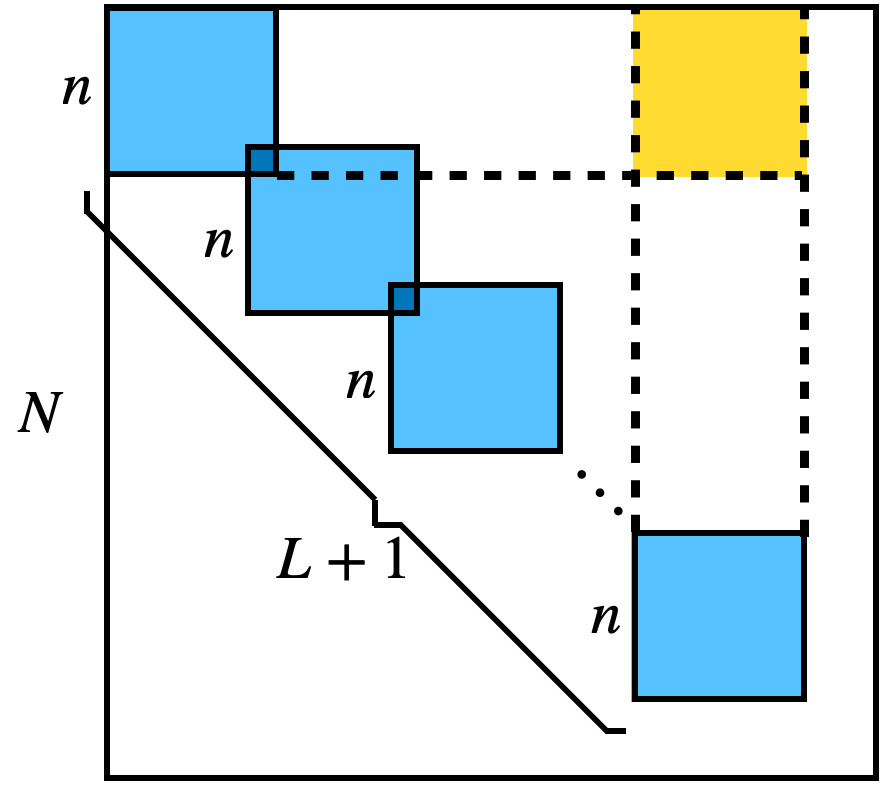
Figure 3: Simulation setting

Recall that, by Theorem 2, the estimation error for $\hat{\mathbf{P}}_{\mathcal{U}_{0},\mathcal{U}_{L}}-\mathbf{P}_{\mathcal{U}_{0},\mathcal{U}_{L}}$can be decomposed into the first order approximation $\mathbf{M}_{\star}:=\mathbf{E}^{(1)}\mathbf{X}_{\mathcal{U}_{1}}(\mathbf{X}_{\mathcal{U}_{1}}^{\top}\mathbf{X}_{\mathcal{U}_{1}})^{-1}\mathbf{X}_{\mathcal{U}_{L}}^{\top}+\mathbf{X}_{\mathcal{U}_{1}}(\mathbf{X}_{\mathcal{U}_{L}}^{\top}\mathbf{X}_{\mathcal{U}_{L}})^{-1}\mathbf{X}_{\mathcal{U}_{L}}^{\top}\mathbf{E}^{({L})}$ and the remainder term $\mathbf{R}^{(0,L)}+\mathbf{S}^{(0,1,\dots,L)}$. Furthermore we also have

$$\|\mathbf{M}_{\star}\|_{\max}\lesssim\frac{(1+\sigma)\log^{1/2}n}{(pqN)^{1/2}},\quad\|\mathbf{R}^{(0,L)}+\mathbf{S}^{(0,1,\dots,L)}\|_{\max}\lesssim L\Big{(}\frac{(1+\sigma)^{2}\log n}{pqN}+\frac{(1+\sigma)\log^{1/2}n}{q^{1/2}\breve{p}^{1/2}pN}\Big{)}$$ (4.1)

with high probability. We compare the error rates for $\|\hat{\mathbf{P}}_{\mathcal{U}_{0},\mathcal{U}_{L}}-\mathbf{P}_{\mathcal{U}_{0},\mathcal{U}_{L}}\|_{\max}$ against $\|\mathbf{M}_{\star}\|_{\max}$ and $\|\mathbf{R}^{(0,L)}+\mathbf{S}^{(0,1,\dots,L)}\|_{\max}$ by varying the value of one parameter among $N$, $p$, $\breve{p}$, $q$, $L$ and $\sigma$ while fixing the values of the remaining parameters. Empirical results for these error rates, averaged over $100$ Monte Carlo replicates, are summarized in Figure 4. We note that the error rates in Figure 4 are consistent with the bounds in Eq. (4.1) obtained by Theorem 2.

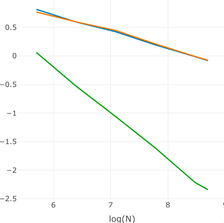
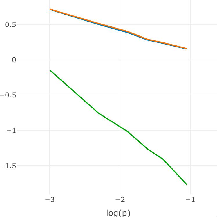
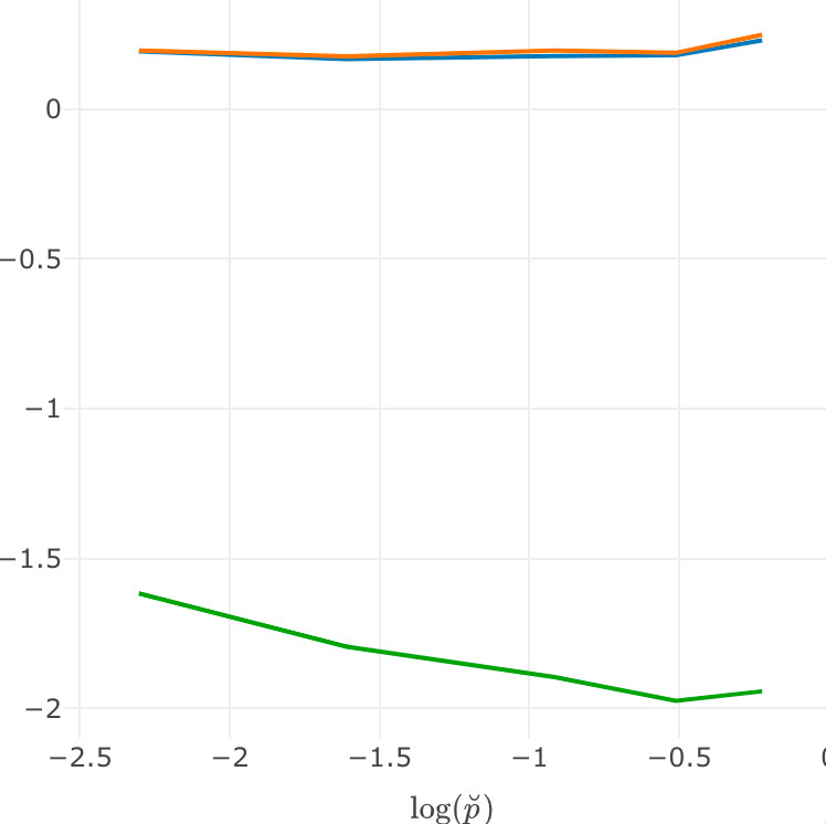
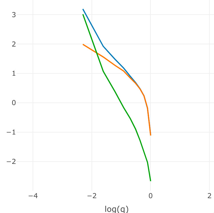
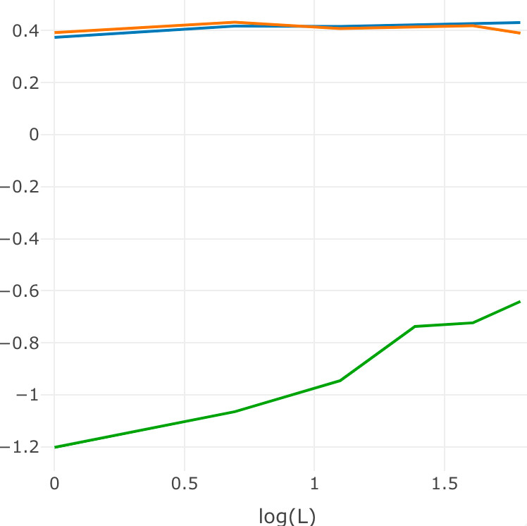
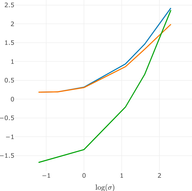
Figure 4: Log-log plot of the empirical error rates for $\|\hat{\mathbf{P}}_{\mathcal{U}_{0},\mathcal{U}_{L}}-\mathbf{P}_{\mathcal{U}_{0},\mathcal{U}_{L}}\|_{\max}$ (blue lines), its first order approximation $\|\mathbf{M}_{\star}\|_{\max}$ (orange lines), and the remainder term $\|\mathbf{R}^{(0,L)}+\mathbf{S}^{(0,1,\dots,L)}\|_{\max}$ (green lines) as we vary the value of a single parameter among $\{N,p,\breve{p},q,L,\sigma\}$ while keeping the values of the remaining parameters fixed (note that we set $\lambda_{\min}=\tfrac{1}{2}N$). Panel (a): vary $N\in\{300,600,1200,2400,4800,6000\}$ for $p=0.3,\breve{p}=0.1,q=0.8,L=2,\sigma=0.5$. Panel (b): vary $p\in\{0.05,0.1,0.15,0.2,0.25,0.35\}$ for $N=2400$, $\breve{p}=0.1$, $q=0.8$, $L=2$, $\sigma=0.5$. Panel (c): vary $\breve{p}\in\{0.1,0.2,0.4,0.6,0.8\}$ for $N=2400$, $p=0.3$, $q=0.8$, $L=2$, $\sigma=0.5$. Panel (d): vary $q\in\{0.1,0.2,\dots,0.9,1\}$ for $N=2400$, $p=0.3$, $\breve{p}=0.1$, $L=2$, $\sigma=0.5$. Panel (e): vary $L\in\{1,2,3,4,5,6\}$ for $N=2400$, $p=0.15$, $\breve{p}=0.1$, $q=0.8$, $\sigma=0.5$. Panel (f): vary $\sigma\in\{0.3,0.5,1,3,5,10\}$ for $N=2400$, $p=0.15$, $\breve{p}=0.1$, $q=0.8$, $L=2$, $\sigma=0.5$. Error rates in each panel are averages based on $100$ independent Monte Carlo replicates.

We next compare the entrywise behavior of $\hat{\mathbf{P}}_{\mathcal{U}_{i_{0}},\mathcal{U}_{i_{L}}}-\mathbf{P}_{\mathcal{U}_{i_{0}},\mathcal{U}_{i_{L}}}$ against the limiting distributions in Theorem 3. In particular, we plot in Figure 5 histograms (based on $1000$ independent Monte Carlo replicates) of the $(i,j)$th entries where $(i,j)\in\{(1,1),(1,2),(1,3)\}$, and it is clear that the empirical distributions in Figure 5 are well approximated by the normal distributions with parameters given in Theorem 3.

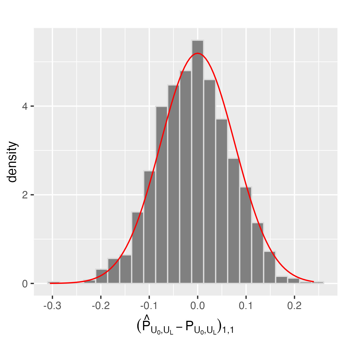
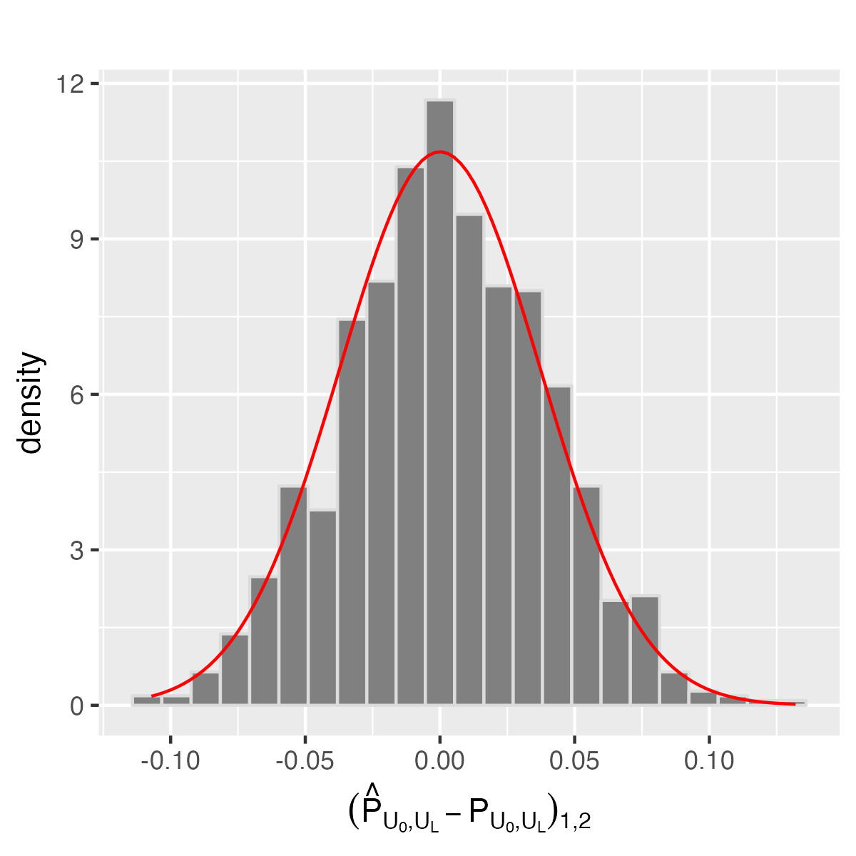
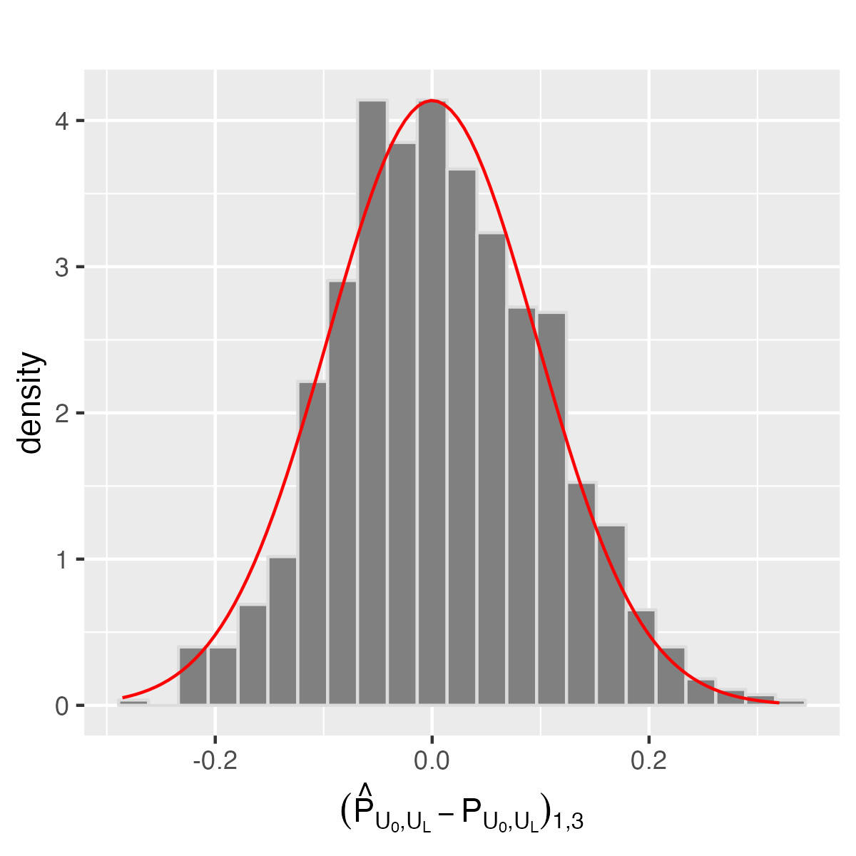
Figure 5: Histograms of the empirical distributions for the $(i,j)$th entry of $\hat{\mathbf{P}}_{\mathcal{U}_{0},\mathcal{U}_{L}}-\mathbf{P}_{\mathcal{U}_{0},\mathcal{U}_{L}}$; here $(i,j)=(1,1)$ (left panel), $(i,j)=(1,2)$ (middle panel), and $(i,j)=(1,3)$ (right panel). These histograms are based on $1000$ independent Monte Carlo replicates where $N=6000$, $p=0.3$, $\breve{p}=0.1$, $q=0.8$, $L=2$, and $\sigma=0.5$. The red lines are pdfs of the normal distributions with parameters given in Theorem 3.

4.2 Comparison with other matrix completion algorithms

We use the same setting as in Section 4.1, but with $N=n+L\times(1-\breve{p})\times n\approx 2200$, so that the observed submatrices fully span the diagonal of the matrix.

We vary $L$ and compare the performance of Algorithm 1 (CMMI) with some existing state-of-art low-rank matrix completion algorithms, including generalized spectral regularization (GSR) (Mazumder et al., 2010), fast alternating least squares (FALS) (Hastie et al., 2015), singular value thresholding (SVT) (Cai et al., 2010), universal singular value thresholding (USVT) (Chatterjee, 2015), iterative regression against right singular vectors (IRRSV) (Troyanskaya et al., 2001). Note that increasing $L$ leads to more observed submatrices but, as each submatrix is of smaller dimensions, the total number of observed entries decreases with $L$ at rate of $N^{2}q/L$. Our performance metric for recovering the yellow unknown block is in terms of the relative Frobenius norm error $\|\hat{\mathbf{P}}_{\mathcal{U}_{0},\mathcal{U}_{L}}-\mathbf{P}_{\mathcal{U}_{0},\mathcal{U}_{L}}\|_{F}/\|\mathbf{P}_{\mathcal{U}_{0},\mathcal{U}_{L}}\|_{F}$. Plots of the error rates (averaged over $100$ independent Monte Carlo replicates) for different algorithms and their running times are presented in the left and right panels of Figure 6, respectively. Figure 6 shows that CMMI outperforms all competing methods in terms of both recovery accuracy and computational efficiency.

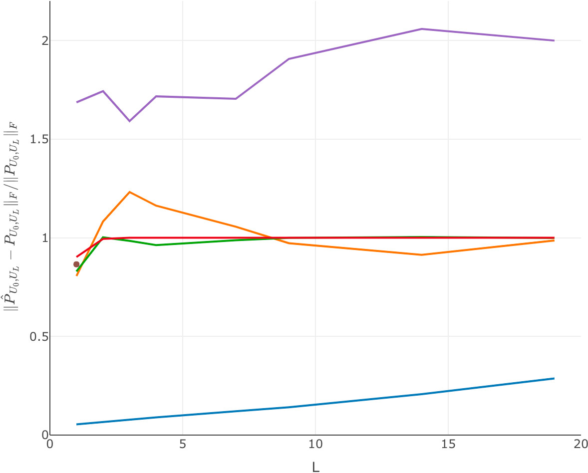
Figure 6: The left panel reports empirical errors $\|\hat{\mathbf{P}}_{\mathcal{U}_{0},\mathcal{U}_{L}}-\mathbf{P}_{\mathcal{U}_{0},\mathcal{U}_{L}}\|_{F}/\|\mathbf{P}_{\mathcal{U}_{0},\mathcal{U}_{L}}\|_{F}$ for CMMI and other matrix completion algorithms as we vary $L\in\{1,2,3,4,7,9,14,19\}$ while fixing $N\approx 2200$, $\breve{p}=0.1$, $q=0.8$, $\sigma=0.5$. The results are averaged over $100$ independent Monte Carlo replicates. Note that the averaged relative $F$-norm errors of IRRSV are $\{0.9,5.6,21.5,24.7,32.7,66.6,1146.3,325.6\}$ and some of these values are too large to be displayed in this panel. Running time of each algorithm (in log-scale) using a machine with 10 cores and 394 GB RAM are reported in the right panel.

4.3 Performance of CMMI with minimal overlap

We now examine the performance of CMMI when the overlap between the submatrices are very small. More specifically, we use the setting from Section 4.2 with $L=2$ and $|\mathcal{U}_{0}\cap\mathcal{U}_{1}|=|\mathcal{U}_{1}\cap\mathcal{U}_{2}|=3$; as $\mathrm{rk}(\mathbf{P})=3$, this is the smallest overlap for which the latent positions for the $\{\hat{\mathbf{X}}^{(i)}\}_{i=0}^{L}$ can still be aligned. We fix $q=0.8,\sigma=0.5$ and compute the estimation error $\|\hat{\mathbf{P}}_{\mathcal{U}_{0},\mathcal{U}_{L}}-\mathbf{P}_{\mathcal{U}_{0},\mathcal{U}_{L}}\|_{\max}$ for several values of $n$. The results are summarized in Figure 7. Note that the slope of the line in the left panel of Figure 7 is approximately the same as the theoretical error rate of $\|\hat{\mathbf{P}}_{\mathcal{U}_{0},\mathcal{U}_{L}}-\mathbf{P}_{\mathcal{U}_{0},\mathcal{U}_{L}}\|_{\max}\lesssim n^{-1/2}\log^{1/2}{n}$ in Remark 6. In summary, CMMI can integrate arbitrarily large submatrices even with very limited overlap.

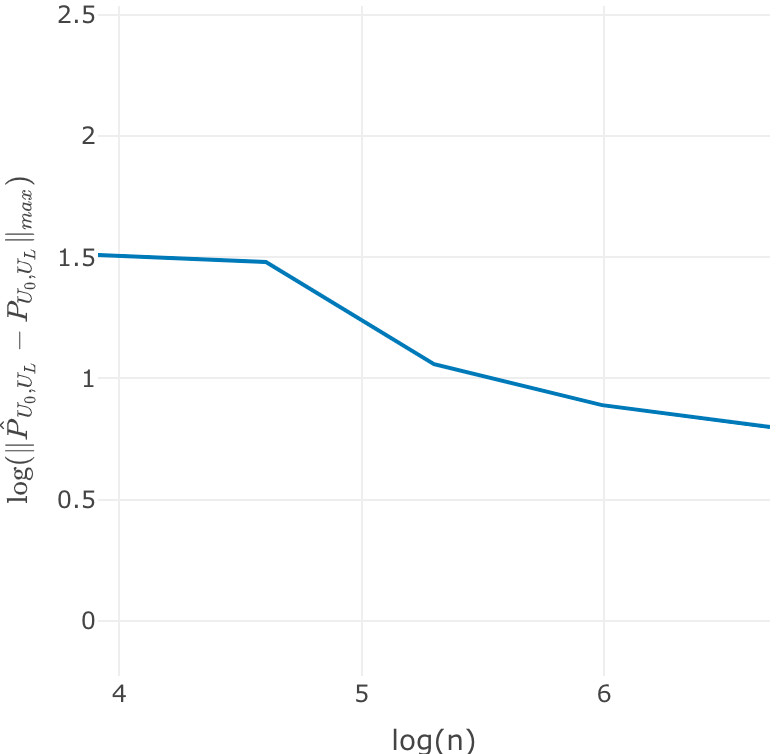
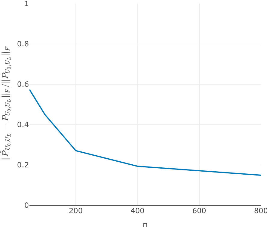
Figure 7: The left panel is a log-log plot of the empirical error rate for $\|\hat{\mathbf{P}}_{\mathcal{U}_{0},\mathcal{U}_{L}}-\mathbf{P}_{\mathcal{U}_{0},\mathcal{U}_{L}}\|_{\max}$ as we vary the values of $n\in\{50,100,200,400,800\}$ while fixing the overlap size as $d=3$, with $L=2$, $q=0.8$, and $\sigma=0.5$. The right panel reports the empirical error rate for $\|\hat{\mathbf{P}}_{\mathcal{U}_{0},\mathcal{U}_{L}}-\mathbf{P}_{\mathcal{U}_{0},\mathcal{U}_{L}}\|_{F}/\|\mathbf{P}_{\mathcal{U}_{0},\mathcal{U}_{L}}\|_{F}$. The errors are based on $100$ independent Monte Carlo replicates.

5 Real Data Experiments

We compare the performance of CMMI against other matrix completion algorithms on the MNIST database of grayscale images and MEDLINE database of co-occurrences citations.

5.1 MNIST

The MNIST database consists of $60000$ grayscale images of handwritten digits for the numbers $0$ through $9$. Each image is of size $28\times 28$ pixels and can be viewed as a vector in $\{0,1,\dots,255\}^{784}$. Let $\mathbf{Y}$ denote the $60000\times 784$ matrix whose rows represent these images, where each row is normalized to be of unit norm. We consider a chain of $L+1$ overlapping blocks, each block corresponding to a partially observed (cosine) kernel matrix for some subset of $n=1000$ images. More specifically,

1. for each $0\leq i\leq L$ we generate a $n\times 784$ matrix $\mathbf{Y}^{(i)}$ whose rows are sampled independently and uniformly from rows of $\mathbf{Y}$ corresponding to one of the digits $\{0,1,2\}$, with the last $n\breve{p}$ rows of $\mathbf{Y}^{(i-1)}$ and the first $n\breve{p}$ rows of $\mathbf{Y}^{(i)}$ having the same labels;

2. we set $\mathbf{P}^{(i)}=\mathbf{Y}^{(i)}\mathbf{Y}^{(i)\top}$ for all $0\leq i\leq L$;

3. finally, $\mathbf{A}^{(i)}=\mathbf{P}^{(i)}\circ\bm{\Omega}^{(i)}$ where $\bm{\Omega}^{(i)}$ is a $n\times n$ symmetric matrix whose upper triangular entries are i.i.d. Bernoulli random variables with success probability $q$.

Given above collection of $\{\mathbf{A}^{(i)}\}_{0\leq i\leq L}$, we compare the accuracy for jointly clustering the images in the first and last blocks. In particular, for CMMI we first construct an embedding $\hat{\mathbf{X}}^{(i)}\in\mathbb{R}^{n\times d}$ using the $d$ leading scaled eigenvectors of $\mathbf{A}^{(i)}$ for each $0\leq i\leq L$, and align $\hat{\mathbf{X}}^{(0)}$ to $\hat{\mathbf{X}}^{(L)}$ via $\breve{\mathbf{X}}^{(0)}:=\hat{\mathbf{X}}^{(0)}\mathbf{W}^{(0,1)}\cdots\mathbf{W}^{(L-1,L)}$ and $\hat{\mathbf{X}}^{(L)}$. We then concatenate the rows of $\breve{\mathbf{X}}^{(0)}$ and $\hat{\mathbf{X}}^{(L)}$ into a $2n\times d$ matrix $\mathbf{Z}^{(0,L)}$ and cluster the rows of $\mathbf{Z}^{(0,L)}$ into $3$ clusters using $K$-means. Finally we compare the accuracy of the cluster assignment against the true labels $\ell\in\{0,1,2\}$ using Adjusted Rand Index (ARI). Note that ARI values range from $-1$ to $1$, with higher values indicating closer alignment between two sets of labels. For other low-rank matrix completion algorithms, we first reconstruct $\mathbf{P}$ from $\{\mathbf{A}^{(i)}\}_{i=0}^{L}$. Letting $\hat{\mathbf{P}}$ denote the resulting estimate, we find $\hat{\mathbf{X}}$ such that $\hat{\mathbf{X}}\hat{\mathbf{X}}^{\top}$ is the best rank-$d$ approximation to $\hat{\mathbf{P}}$ in Frobenius norm (among all positive semidefinite matrices). We then subset $\hat{\mathbf{X}}$ to keep only $2n$ rows corresponding to images in $\mathbf{A}^{(0)}$ and $\mathbf{A}^{(L)}$, and finally cluster these $2n$ rows into $3$ clusters using $K$-means and compute the ARI of the resulting cluster assignments.

Comparisons between the ARIs of CMMI and other matrix completion algorithms, for different numbers of submatrices $L$, are summarized in Figure 8. Note that the black dotted line in the left panel of Figure 8 are ARIs when applying $K$-means directly on $\mathbf{Y}^{(0)}$ and $\mathbf{Y}^{(L)}$, and thus represent the best possible clustering accuracy. We observe that CMMI outperforms all competing methods on this dataset, and its ARIs remain close to optimal even as $L$ increases. Finally, the right panel of Figure 8 shows that the running time for CMMI is orders of magnitude smaller than that of other algorithms.

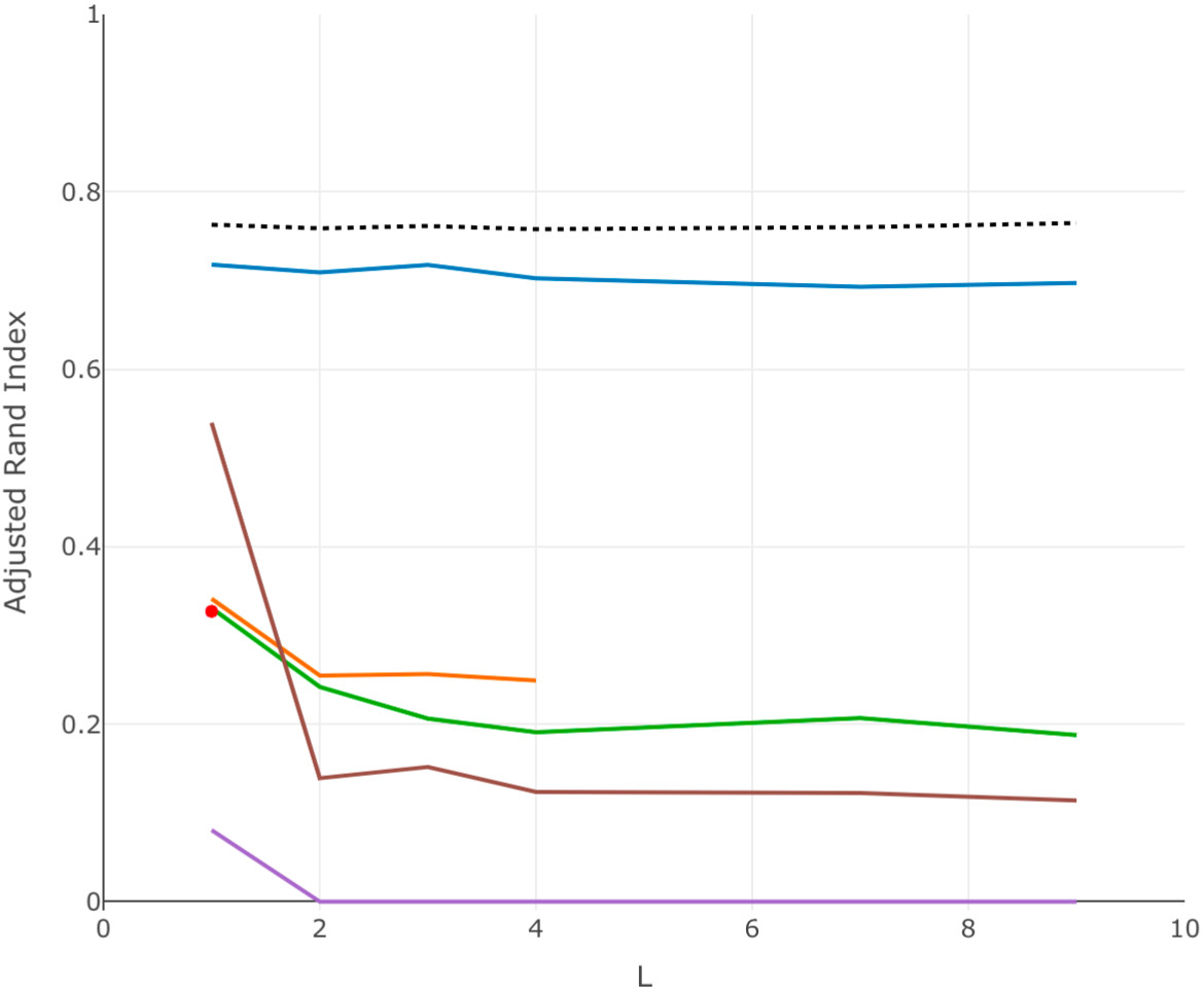
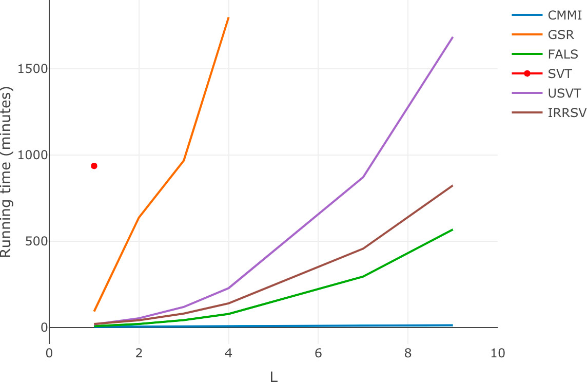
Figure 8: The left panel reports ARIs for joint clustering of $(\hat{\mathbf{X}}^{(0)},\hat{\mathbf{X}}^{(L)})$ for subsets of the MNIST dataset using CMMI and other low-rank matrix completion algorithms. In particular, we vary $L\in\{1,2,3,4,7,9\}$ while fixing $n=1000$, $\breve{p}=0.1$, $q=0.8$, $d=2$. The black dotted line is the ARIs obtained by clustering directly on the original data (i.e, observed without noise nor missing entries). The right panel reports running time of these algorithms on a standard laptop with $8$ computing threads. The results in each panel are based on $100$ independent Monte Carlo replicates. We only evaluate the performance of GSR for $L\leq 4$ and SVT for $L=1$, as these algorithms are computationally prohibitive with even slight increases in $L$.

5.2 MEDLINE co-occurrences

The MEDLINE co-occurrences database (National Library of Medicine, 2023) summarizes the MeSH Descriptors that occur together in MEDLINE citations from the MEDLINE/PubMed Baseline over a duration of several years. A standard approach for handling this type of data is to first transform the (normalized) co-occurrence counts into pointwise mutual information (PMI), an association measure widely used in natural language processing (Church and Hanks, 1990; Lu et al., 2023). More specifically, the PMI between two concepts $x$ and $y$ is defined as $\mathrm{PMI}(x,y)=\log\tfrac{\mathbb{P}(x,y)}{\mathbb{P}(x)\mathbb{P}(y)},$ where $\mathbb{P}(x)$ and $\mathbb{P}(y)$ are the (marginal) occurrence probability of $x$ and $y$, and $\mathbb{P}(x,y)$ is the (joint) co-occurrence probability of $x$ and $y$.

For our analysis of the MEDLINE data, we first select $N=7486$ clinical concepts which were most frequently cited during the twelve years period from $2011$ to $2022$, and construct the total PMI matrix $\mathbf{P}\in\mathbb{R}^{N\times N}$ between these concepts. Next we split the dates into $L+1$ time intervals of equal length, and for each time interval $0\leq i\leq L$ we construct the individual PMI matrix $\mathbf{P}^{(i)}\in\mathbb{R}^{N\times N}$. We randomly sample, for each interval, a subset $\mathcal{U}_{i}$ of $n=1000$ concepts from those $N=7486$ cited concepts such that $|\mathcal{U}_{i-1}\cap\mathcal{U}_{i}|=100$ for all $1\leq i\leq L$. Finally we set $\mathbf{A}^{(i)}=\mathbf{P}^{(i)}_{\mathcal{U}_{i},\mathcal{U}_{i}}$ as the principal submatrix of $\mathbf{P}^{(i)}$ induced by $\mathcal{U}_{i}$. The collection $\{\mathbf{A}^{(i)}\}_{0\leq i\leq L}$ forms a chain of perturbed overlapping submatrices of $\mathbf{P}$.

Given $\{\mathbf{A}^{(i)}\}$, we apply CMMI and other low-rank matrix completion algorithms to construct $\hat{\mathbf{P}}_{\mathcal{U}_{i_{0}},\mathcal{U}_{i_{L}}}$ for the PMIs between clinical concepts in $\mathcal{U}_{0}$ and those in $\mathcal{U}_{L}$ in the total PMI matrix $\mathbf{P}$. Note that we specify $d=23$ for both CMMI and FALS, where this choice is based on applying the dimensionality selection procedure of Zhu and Ghodsi (2006) to $\mathbf{P}$. In contrast we set $d=3$ for GSR as its running time increase substantially for larger values of $d$. The values of $d$ for SVT and USVT are not specified, as both algorithms automatically determine $d$ using their respective eigenvalue thresholding procedures. We then measure the similarities between the estimated PMIs in $\hat{\mathbf{P}}_{\mathcal{U}_{0},\mathcal{U}_{L}}$ and the true total PMIs in $\mathbf{P}_{\mathcal{U}_{0},\mathcal{U}_{L}}$ in terms of the Spearman’s rank correlation $\rho$ (note that, for ease of exposition, we only compare PMIs for pairs of concepts with positive co-occurrence). The Spearman’s $\rho$ between two set of vectors takes value in $[-1,1]$ with $1$ (resp. $-1$) denoting perfect monotone increasing (resp. decreasing) relationship and $0$ suggesting no relationship. The results, averaged over $100$ independent Monte Carlo replicates, are summarized in Figure 9. CMMI outperforms competing algorithms in terms of both accuracy and computational efficiency.

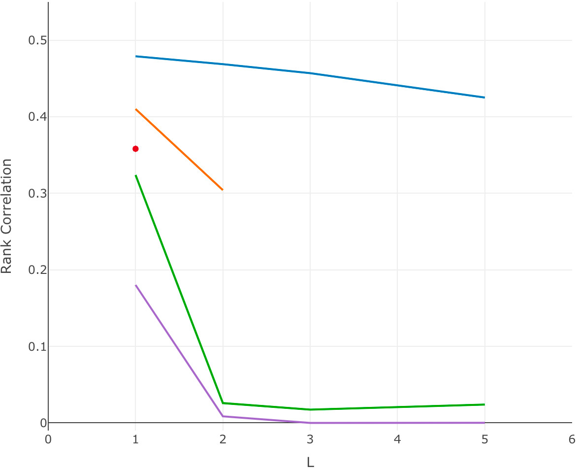
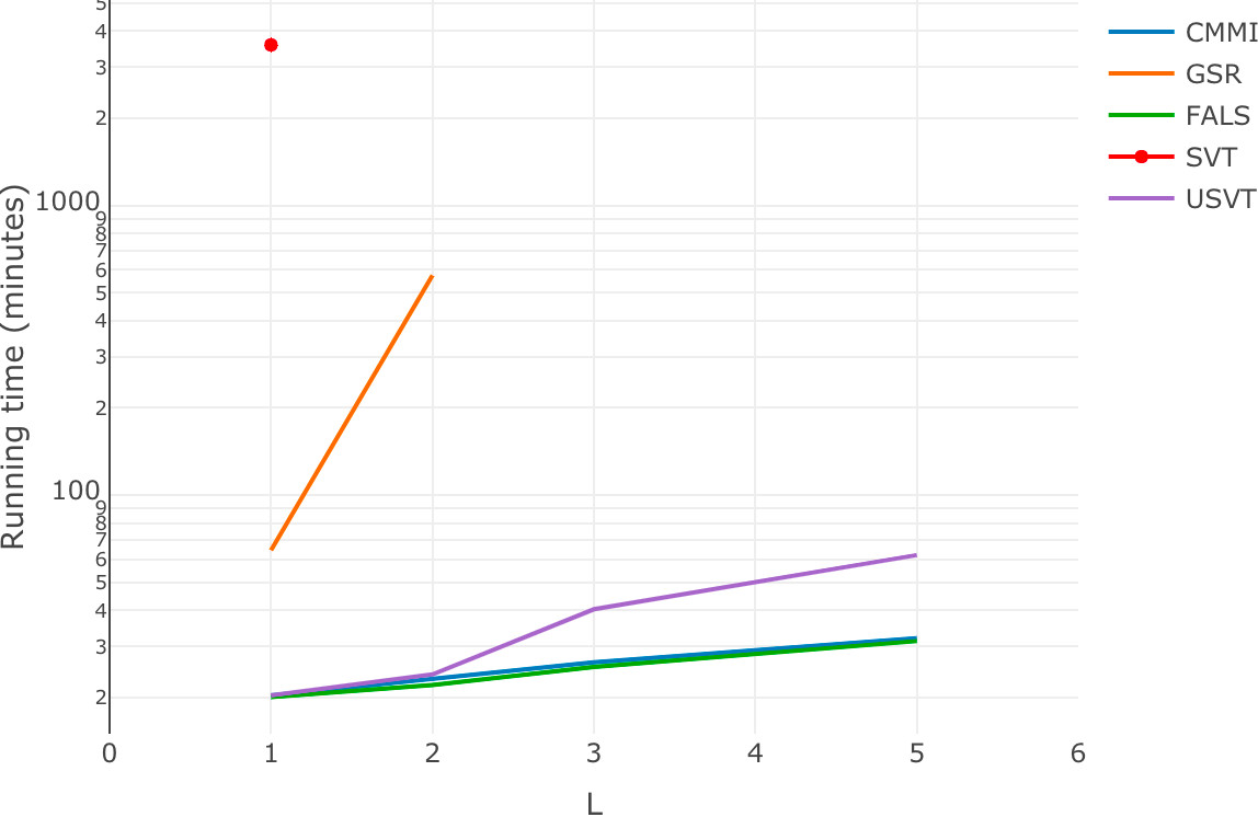
Figure 9: The left panel reports empirical estimates of Spearman’s rank correlations for CMMI and other low-rank matrix completion algorithms as $L$ changes; we were not able to evaluate IRRSV in this experiment due to the sparse nature of the co-occurence matrix (about 60% zero entries in $\mathbf{P}$). In particular, we vary $L=\{1,2,3,5\}$ while fixing $n=1000$ and $\breve{p}=0.1.$ The right panel reports running time (in log-scale) of these algorithms on a machine with $5$ cores and $394$ GB RAM. The results in each panel are averaged over $100$ independent Monte Carlo replicates.

6 Extensions to Indefinite or Asymmetric Matrices

We now describe how the methodologies presented in this paper can be extended to block-wise data integration of symmetric indefinite matrices and asymmetric/rectangular matrices.

6.1 CMMI for symmetric indefinite matrices

Suppose $\mathbf{P}\in\mathbb{R}^{N\times N}$ is a symmetric indefinite low-rank matrix. Let $d_{+}$ and $d_{-}$ be the number of positive and negative eigenvalues of $\mathbf{P}$ and set $d=d_{+}+d_{-}\ll N$. We denote the non-zero eigenvalues of $\mathbf{P}$ by $\lambda_{1}(\mathbf{P})\geq\dots\geq\lambda_{d_{+}}(\mathbf{P})>0>\lambda_{n-d_{-}+1}(\mathbf{P})\geq\dots\geq\lambda_{n}(\mathbf{P}).$ Let $\bm{\Lambda}_{+}:=\mathrm{diag}(\lambda_{1}(\mathbf{P}),\dots,\lambda_{d_{+}}(\mathbf{P}))$, $\bm{\Lambda}_{-}:=\mathrm{diag}(\lambda_{n-d_{-}+1}(\mathbf{P}),\dots,\lambda_{n}(\mathbf{P}))$, and the orthonormal columns of $\mathbf{U}_{+}\in\mathbb{R}^{N\times d_{+}}$ and $\mathbf{U}_{-}\in\mathbb{R}^{N\times d_{-}}$ constitute the corresponding eigenvectors. Then the eigen-decomposition of $\mathbf{P}$ is $\mathbf{U}\bm{\Lambda}\mathbf{U}^{\top}$, where $\bm{\Lambda}:=\mathrm{diag}(\bm{\Lambda}_{+},\bm{\Lambda}_{-})$ and $\mathbf{U}:=[\mathbf{U}_{+},\mathbf{U}_{-}]$.

Then $\mathbf{P}$ can be written as $\mathbf{P}=\mathbf{X}\mathbf{I}_{d_{+},d_{-}}\mathbf{X}^{\top}$ with $\mathbf{X}=\mathbf{U}|\bm{\Lambda}|^{1/2}$, and thus the rows of $\mathbf{X}$ represent the latent positions for the entities. For any $i\in[K]$, let $\mathcal{U}_{i}\subseteq[N]$ denote the set of entities contained in the $i$th source, and let $\mathbf{P}^{(i)}$ be the corresponding population matrix. We then have $\mathbf{P}^{(i)}=\mathbf{P}_{\mathcal{U}_{i},\mathcal{U}_{i}}=\mathbf{U}_{\mathcal{U}_{i}}\bm{\Lambda}\mathbf{U}_{\mathcal{U}_{i}}^{\top}=\mathbf{X}_{\mathcal{U}_{i}}\mathbf{I}_{d_{+},d_{-}}\mathbf{X}_{\mathcal{U}_{i}}^{\top}.$ For each observed submatrix $\mathbf{A}^{(i)}$ on $\mathcal{U}_{i}$, we compute the estimated latent position matrix $\hat{\mathbf{X}}^{(i)}=\hat{\mathbf{U}}^{(i)}|\hat{\bm{\Lambda}}^{(i)}|^{1/2}$. Here $\hat{\bm{\Lambda}}^{(i)}:=\mathrm{diag}(\hat{\bm{\Lambda}}_{+}^{(i)},\hat{\bm{\Lambda}}_{-}^{(i)})\in\mathbb{R}^{d\times d}$ and $\hat{\bm{\Lambda}}_{+}^{(i)}$, $\hat{\bm{\Lambda}}_{-}^{(i)}$ contain the $d_{+}$ largest positive and $d_{-}$ largest (in-magnitude) negative eigenvalues of $\mathbf{A}^{(i)}$, respectively. $\hat{\mathbf{U}}^{(i)}:=[\hat{\mathbf{U}}_{+}^{(i)},\hat{\mathbf{U}}_{-}^{(i)}]$ contains the corresponding eigenvectors.

We start with the noiseless case to illustrate the main idea. Consider $2$ overlapping block-wise submatrices $\mathbf{P}^{(1)}$ and $\mathbf{P}^{(2)}$ as shown in Figure 1. Now

$$\mathbf{X}_{\mathcal{U}_{1}}\mathbf{I}_{d_{+},d_{-}}\mathbf{X}_{\mathcal{U}_{1}}^{\top}=\mathbf{P}^{(1)}=\mathbf{X}^{(1)}\mathbf{I}_{d_{+},d_{-}}\mathbf{X}^{(1)\top},\quad\mathbf{X}_{\mathcal{U}_{2}}\mathbf{I}_{d_{+},d_{-}}\mathbf{X}_{\mathcal{U}_{2}}^{\top}=\mathbf{P}^{(2)}=\mathbf{X}^{(2)}\mathbf{I}_{d_{+},d_{-}}\mathbf{X}^{(2)\top},$$

and hence there exist matrices $\mathbf{W}^{(1)}\in\mathcal{O}_{d_{+},d_{-}}$ and $\mathbf{W}^{(2)}\in\mathcal{O}_{d_{+},d_{-}}$ such that

$$\mathbf{X}_{\mathcal{U}_{1}}=\mathbf{X}^{(1)}\mathbf{W}^{(1)},\quad\mathbf{X}_{\mathcal{U}_{2}}=\mathbf{X}^{(2)}\mathbf{W}^{(2)}.$$ (6.1)

Here $\mathcal{O}_{d_{+},d_{-}}:=\{\mathbf{O}\in\mathbb{R}^{d\times d}\mid\mathbf{O}\mathbf{I}_{d_{+},d_{-}}\mathbf{O}^{\top}=\mathbf{I}_{d_{+},d_{-}}\}$ is the indefinite orthogonal group. Eq. (6.1) implies

$$\mathbf{P}_{\mathcal{U}_{1},\mathcal{U}_{2}} =\mathbf{X}_{\mathcal{U}_{1}}\mathbf{I}_{d_{+},d_{-}}\mathbf{X}_{\mathcal{U}_{2}}^{\top}=\mathbf{X}^{(1)}\mathbf{W}^{(1)}\mathbf{I}_{d_{+},d_{-}}\mathbf{W}^{(2)\top}\mathbf{X}^{(2)\top}=\mathbf{X}^{(1)}\mathbf{W}^{(1)}(\mathbf{W}^{(2)})^{-1}\mathbf{I}_{d_{+},d_{-}}\mathbf{X}^{(2)\top}$$

$$=\mathbf{X}^{(1)}\mathbf{W}^{(1,2)}\mathbf{I}_{d_{+},d_{-}}\mathbf{X}^{(2)\top},$$

where we define $\mathbf{W}^{(1,2)}:=\mathbf{W}^{(1)}(\mathbf{W}^{(2)})^{-1}\in\mathcal{O}_{d_{+},d_{-}}$ and we can recover $\mathbf{W}^{(1,2)}$ by aligning the latent positions for overlapping entities,

$$\mathbf{W}^{(1,2)}=\underset{\mathbf{O}\in\mathcal{O}_{d_{+},d_{-}}}{\operatorname{argmin}}\|\mathbf{X}^{(1)}_{\langle\mathcal{U}_{1}\cap\mathcal{U}_{2}\rangle}\mathbf{O}-\mathbf{X}^{(2)}_{\langle\mathcal{U}_{1}\cap\mathcal{U}_{2}\rangle}\|_{F}.$$ (6.2)

If $\mathrm{rk}(\mathbf{P}_{\mathcal{U}_{1}\cap\mathcal{U}_{2},\mathcal{U}_{1}\cap\mathcal{U}_{2}})=d$ then $\mathbf{W}^{(1,2)}=(\mathbf{X}^{(1)\top}_{\langle\mathcal{U}_{1}\cap\mathcal{U}_{2}\rangle}\mathbf{X}^{(1)}_{\langle\mathcal{U}_{1}\cap\mathcal{U}_{2}\rangle})^{-1}\mathbf{X}^{(1)\top}_{\langle\mathcal{U}_{1}\cap\mathcal{U}_{2}\rangle}\mathbf{X}^{(2)}_{\langle\mathcal{U}_{1}\cap\mathcal{U}_{2}\rangle}=(\mathbf{X}^{(1)}_{\langle\mathcal{U}_{1}\cap\mathcal{U}_{2}\rangle})^{\dagger}\mathbf{X}^{(2)}_{\langle\mathcal{U}_{1}\cap\mathcal{U}_{2}\rangle}$ is the unique minimizer of Eq. (6.2). Here $(\cdot)^{\dagger}$ denotes the Moore-Penrose pseudoinverse.

Now suppose $\mathbf{A}^{(1)}$ and $\mathbf{A}^{(2)}$ are noisy observations of $\mathbf{P}^{(1)}$ and $\mathbf{P}^{(2)}$. Let $\hat{\mathbf{X}}^{(1)}$ and $\hat{\mathbf{X}}^{(2)}$ be estimates of $\mathbf{X}^{(1)}$ and $\mathbf{X}^{(2)}$ as described above. Then to align $\hat{\mathbf{X}}^{(1)}$ and $\hat{\mathbf{X}}^{(2)}$, we can consider solving the indefinite orthogonal Procrustes problem

$$\mathbf{W}^{(1,2)}=\underset{\mathbf{O}\in\mathcal{O}_{d_{+},d_{-}}}{\operatorname{argmin}}\|\hat{\mathbf{X}}^{(1)}_{\langle\mathcal{U}_{1}\cap\mathcal{U}_{2}\rangle}\mathbf{O}-\hat{\mathbf{X}}^{(2)}_{\langle\mathcal{U}_{1}\cap\mathcal{U}_{2}\rangle}\|_{F}.$$ (6.3)

However, in contrast to the noiseless case, there is no longer an analytical solution to Eq. (6.3). We thus replace Eq. (6.3) with the unconstrained least squares problem

$$\mathbf{W}^{(1,2)}=\underset{\mathbf{O}\in\mathbb{R}^{d\times d}}{\operatorname{argmin}}\|\hat{\mathbf{X}}^{(1)}_{\langle\mathcal{U}_{1}\cap\mathcal{U}_{2}\rangle}\mathbf{O}-\hat{\mathbf{X}}^{(2)}_{\langle\mathcal{U}_{1}\cap\mathcal{U}_{2}\rangle}\|_{F},$$

whose solution is once again $\mathbf{W}^{(1,2)}=(\hat{\mathbf{X}}^{(1)}_{\langle\mathcal{U}_{1}\cap\mathcal{U}_{2}\rangle})^{\dagger}\hat{\mathbf{X}}^{(2)}_{\langle\mathcal{U}_{1}\cap\mathcal{U}_{2}\rangle}$. Given $\mathbf{W}^{(1,2)}$, we estimate $\mathbf{P}_{\mathcal{U}_{1},\mathcal{U}_{2}}$ by $\hat{\mathbf{P}}_{\mathcal{U}_{1},\mathcal{U}_{2}}=\hat{\mathbf{X}}^{(1)}\mathbf{W}^{(1,2)}\mathbf{I}_{d_{+},d_{-}}\hat{\mathbf{X}}^{(2)\top}.$ Extending the above idea to a chain of overlapping submatrices is also straightforward; see Section B.1 in the supplementary material for the detailed algorithm and simulation results.

The following result extends Theorem 2 to the indefinite setting. We note that the main difference in this extension is in the upper bound for $\mathbf{S}^{(i_{0},i_{1},\dots,i_{L})}$ and this is due to the fact that the least square transformations $\{(\hat{\mathbf{X}}^{(i_{\ell-1})}_{\langle\mathcal{U}_{i_{\ell-1}}\cap\mathcal{U}_{i_{\ell}}\rangle})^{\dagger}\hat{\mathbf{X}}^{(i_{\ell})}_{\langle\mathcal{U}_{i_{\ell-1}}\cap\mathcal{U}_{i_{\ell}}\rangle}\}_{1\leq\ell\leq L}$ have spectral norms that can be smaller or larger than $1$, and the accumulated error induced by these transformations need not grow linearly with $L$. Finally if $L=1$ then the bounds in Theorem 4 are almost identical to those in Theorem 1, but with a slightly different definition for $\alpha_{i,j}$.

Theorem 4.

Consider a chain of overlapping submatrices $(\mathbf{A}^{(i_{0})},\dots,\mathbf{A}^{(i_{L})})$ where, for each $0\leq\ell\leq L$, $\mathbf{P}^{(i_{\ell})}$ has $d_{+}$ positive eigenvalues and $d_{-}$ negative eigenvalues, satisfying Assumption 1. Set $d=d_{+}+d_{-}$. Here we define $\mu_{i}:=\lambda_{\min}(\mathbf{X}^{\top}_{\mathcal{U}_{i},\mathcal{U}_{i}}\mathbf{X}_{\mathcal{U}_{i},\mathcal{U}_{i}})/n_{i}$, $\gamma_{i}:=(\|\mathbf{P}_{\mathcal{U}_{i},\mathcal{U}_{i}}\|_{\max}+\sigma_{i})\log^{1/2}n_{i}$ for any $i$, and suppose $\frac{\gamma_{i}}{(q_{i}n_{i}\mu_{i})^{1/2}}\lesssim\|\mathbf{X}^{(i)}\|_{2\to\infty}$ for $i\in\{i_{0},i_{L}\}$. For all overlaps $1\leq\ell\leq L$, suppose $\mathrm{rk}(\mathbf{P}^{(i_{\ell})}_{\mathcal{U}_{i_{\ell-1}}\cap\mathcal{U}_{i_{\ell}},\mathcal{U}_{i_{\ell-1}}\cap\mathcal{U}_{i_{\ell}}})=d$, and define

$$\vartheta_{i_{\ell-1},i_{\ell}} :=\lambda_{\max}(\mathbf{X}^{(i_{\ell})\top}_{\langle\mathcal{U}_{i_{\ell-1}}\cap\mathcal{U}_{i_{\ell}}\rangle}\mathbf{X}^{(i_{\ell})}_{\langle\mathcal{U}_{i_{\ell-1}}\cap\mathcal{U}_{i_{\ell}}\rangle}),\quad\theta_{i_{\ell-1},i_{\ell}}:=\lambda_{\min}(\mathbf{X}^{(i_{\ell-1})\top}_{\langle\mathcal{U}_{i_{\ell-1}}\cap\mathcal{U}_{i_{\ell}}\rangle}\mathbf{X}^{(i_{\ell-1})}_{\langle\mathcal{U}_{i_{\ell-1}}\cap\mathcal{U}_{i_{\ell}}\rangle}),$$

$$\alpha_{i_{\ell-1},i_{\ell}}:= \frac{n_{i_{\ell-1},i_{\ell}}\gamma_{i_{\ell-1}}\gamma_{i_{\ell}}}{\theta_{{i_{\ell-1}},{i_{\ell}}}(q_{i_{\ell-1}}n_{i_{\ell-1}}\mu_{i_{\ell-1}})^{1/2}(q_{i_{\ell}}n_{i_{\ell}}\mu_{i_{\ell}})^{1/2}}+\frac{n_{{i_{\ell-1}},{i_{\ell}}}^{1/2}}{\theta_{{i_{\ell-1}},{i_{\ell}}}^{1/2}}\Bigl{(}\frac{\gamma_{i_{\ell-1}}^{2}}{q_{i_{\ell-1}}n_{i_{\ell-1}}\mu_{i_{\ell-1}}^{3/2}}+\frac{\vartheta_{{i_{\ell-1}},{i_{\ell}}}^{1/2}\gamma_{i_{\ell}}^{2}}{\theta_{{i_{\ell-1}},{i_{\ell}}}^{1/2}q_{i_{\ell}}n_{i_{\ell}}\mu_{i_{\ell}}^{3/2}}\Bigr{)}$$

$$+\frac{n_{{i_{\ell-1}},{i_{\ell}}}\vartheta_{{i_{\ell-1}},{i_{\ell}}}^{1/2}\gamma_{i_{\ell-1}}^{2}}{\theta_{{i_{\ell-1}},{i_{\ell}}}^{3/2}q_{i_{\ell-1}}n_{i_{\ell-1}}\mu_{i_{\ell-1}}}+\frac{n_{{i_{\ell-1}},{i_{\ell}}}^{1/2}\|\mathbf{X}^{({i_{\ell-1}})}_{\langle\mathcal{U}_{i_{\ell-1}}\cap\mathcal{U}_{i_{\ell}}\rangle}\|_{2\to\infty}}{\theta_{{i_{\ell-1}},{i_{\ell}}}}\Big{(}\frac{\gamma_{i_{\ell-1}}}{(q_{i_{\ell-1}}n_{i_{\ell-1}}\mu_{i_{\ell-1}})^{1/2}}+\frac{\vartheta_{{i_{\ell-1}},{i_{\ell}}}^{1/2}\gamma_{i_{\ell}}}{\theta_{{i_{\ell-1}},{i_{\ell}}}^{1/2}(q_{i_{\ell}}n_{i_{\ell}}\mu_{i_{\ell}})^{1/2}}\Big{)}.$$

Suppose $\frac{n_{{i_{\ell-1}},{i_{\ell}}}^{1/2}\gamma_{i_{\ell-1}}}{(q_{i_{\ell-1}}n_{i_{\ell-1}}\mu_{i_{\ell-1}})^{1/2}}\ll\theta_{{i_{\ell-1}},{i_{\ell}}}^{1/2}$ for all $1\leq\ell\leq L$. We then have

$$\hat{\mathbf{P}}_{\mathcal{U}_{i_{0}},\mathcal{U}_{i_{L}}}-\mathbf{P}_{\mathcal{U}_{i_{0}},\mathcal{U}_{i_{L}}}=\mathbf{E}^{(i_{0})}\mathbf{X}_{\mathcal{U}_{i_{0}}}(\mathbf{X}_{\mathcal{U}_{i_{0}}}^{\top}\mathbf{X}_{\mathcal{U}_{i_{0}}})^{-1}\mathbf{X}_{\mathcal{U}_{i_{L}}}^{\top}+\mathbf{X}_{\mathcal{U}_{i_{0}}}(\mathbf{X}_{\mathcal{U}_{i_{L}}}^{\top}\mathbf{X}_{\mathcal{U}_{i_{L}}})^{-1}\mathbf{X}_{\mathcal{U}_{i_{L}}}^{\top}\mathbf{E}^{(i_{L})}+\mathbf{R}^{(i_{0},i_{L})}+\mathbf{S}^{(i_{0},i_{1},\dots,i_{L})},$$

where $\mathbf{R}^{(i_{0},i_{L})}$ and $\mathbf{S}^{(i_{0},i_{1},\dots,i_{L})}$ are random matrices satisfying

$$\begin{split}\|\mathbf{R}^{(i_{0},i_{L})}\|_{\max}\lesssim&\Big{(}\frac{\gamma_{i_{0}}^{2}}{q_{i_{0}}n_{i_{0}}\mu_{i_{0}}^{3/2}}+\frac{\gamma_{i_{0}}}{q_{i_{0}}^{1/2}n_{i_{0}}\mu_{i_{0}}^{1/2}}\Big{)}\|\mathbf{X}^{(i_{L})}\|_{2\to\infty}+\Big{(}\frac{\gamma_{i_{L}}^{2}}{q_{i_{L}}n_{i_{L}}\mu_{i_{L}}^{3/2}}+\frac{\gamma_{i_{L}}}{q_{i_{L}}^{1/2}n_{i_{L}}\mu_{i_{L}}^{1/2}}\Big{)}\|\mathbf{X}^{(i_{0})}\|_{2\to\infty}\\ &+\frac{\gamma_{i_{0}}\gamma_{i_{L}}}{(q_{i_{0}}n_{i_{0}}\mu_{i_{0}})^{1/2}(q_{i_{L}}n_{i_{L}}\mu_{i_{L}})^{1/2}},\end{split}$$

$$\|\mathbf{S}^{(i_{0},i_{1},\dots,i_{L})}\|_{\max}\lesssim a_{L}\|\mathbf{X}^{(i_{0})}\|_{2\to\infty}\cdot\|\mathbf{X}^{(i_{L})}\|_{2\to\infty}$$

with high probability. Here $a_{L}$ is a quantity defined recursively by $a_{1}=\alpha_{i_{0},i_{1}}$ and

$$\quad a_{\ell}=a_{\ell-1}\cdot\Bigl{(}\alpha_{i_{\ell-1},i_{\ell}}+\Bigl{[}\frac{\vartheta_{i_{\ell-1},i_{\ell}}}{\theta_{i_{\ell-1},i_{\ell}}}\Bigr{]}^{1/2}\Bigr{)}+\Big{\|}\prod_{k=1}^{\ell-1}\bigl{(}\mathbf{X}_{\langle\mathcal{U}_{i_{k-1}}\cap\mathcal{U}_{i_{k}}\rangle}^{(i_{k-1})}\bigr{)}^{\dagger}\mathbf{X}_{\langle\mathcal{U}_{i_{k-1}}\cap\mathcal{U}_{i_{k}}\rangle}^{(i_{k})}\Bigr{\|}\cdot\alpha_{i_{\ell-1},i_{\ell}}$$

for $2\leq\ell\leq L$.

6.2 CMMI for asymmetric matrices

Data integration for asymmetric matrices has many applications including genomic data integration (Maneck et al., 2011; Cai et al., 2016), single-cell data integration (Stuart et al., 2019; Ma et al., 2024). Suppose $\mathbf{P}\in\mathbb{R}^{N\times M}$ is a low-rank matrix. Let $d$ be the rank of $\mathbf{P}$, and write the singular decomposition of $\mathbf{P}$ as $\mathbf{P}=\mathbf{U}\bm{\Sigma}\mathbf{V}^{\top},$ where $\bm{\Sigma}\in\mathbb{R}^{d\times d}$ is a diagonal matrix whose diagonal entries are composed of the singular values of $\mathbf{P}$ in a descending order, and orthonormal columns of $\mathbf{U}\in\mathbb{R}^{N\times d}$ and $\mathbf{V}\in\mathbb{R}^{M\times d}$ constitute the corresponding left and right singular vectors, respectively. The left and right latent position matrices associated to the entities can be represented by $\mathbf{X}=\mathbf{U}\bm{\Sigma}^{1/2}\in\mathbb{R}^{N\times d}$ and $\mathbf{Y}=\mathbf{V}\bm{\Sigma}^{1/2}\in\mathbb{R}^{M\times d}$, respectively. For the $i$th source we denote the index set of the entities for rows and columns by $\mathcal{U}_{i}\subseteq[N]$ and $\mathcal{V}_{i}\subseteq[M]$, and let $\mathbf{P}^{(i)}=\mathbf{P}_{\mathcal{U}_{i},\mathcal{V}_{i}}=\mathbf{U}_{\mathcal{U}_{i}}\bm{\Sigma}\mathbf{V}_{\mathcal{V}_{i}}^{\top}=\mathbf{X}_{\mathcal{U}_{i}}\mathbf{Y}_{\mathcal{V}_{i}}^{\top}.$ For each noisily observed realization $\mathbf{A}^{(i)}$ of $\mathbf{P}^{(i)}$, we obtain the estimated left latent positions $\hat{\mathbf{X}}^{(i)}=\hat{\mathbf{U}}^{(i)}(\hat{\bm{\Sigma}}^{(i)})^{1/2}$ for entities in $\mathcal{U}_{i}$ and right latent positions $\hat{\mathbf{Y}}^{(i)}=\hat{\mathbf{V}}^{(i)}(\hat{\bm{\Sigma}}^{(i)})^{1/2}$ for entities in $\mathcal{V}_{i}$.

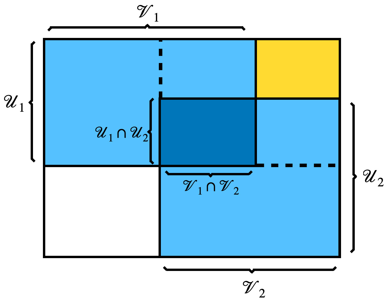
Figure 10: A pair of overlapping observed submatrices of an asymmetric/rectangular matrix

Let $\mathbf{P}^{(1)}$ and $\mathbf{P}^{(2)}$ be two overlapping submatrices shown in Figure 10 without noise or missing entries. Suppose $\mathrm{rank}(\mathbf{P}^{(1)})=\mathrm{rank}(\mathbf{P}^{(2)})=\mathrm{rank}(\mathbf{X}_{\mathcal{U}_{1}\cap\mathcal{U}_{2}})=\mathrm{rank}(\mathbf{Y}_{\mathcal{V}_{1}\cap\mathcal{V}_{2}})=d$. Now

$$\mathbf{X}_{\mathcal{U}_{1}}\mathbf{Y}_{\mathcal{V}_{1}}^{\top}=\mathbf{P}_{\mathcal{U}_{1},\mathcal{V}_{1}}=\mathbf{P}^{(1)}=\mathbf{X}^{(1)}\mathbf{Y}^{(1)\top},\quad\mathbf{X}_{\mathcal{U}_{2}}\mathbf{Y}_{\mathcal{V}_{2}}^{\top}=\mathbf{P}_{\mathcal{U}_{2},\mathcal{V}_{2}}=\mathbf{P}^{(2)}=\mathbf{X}^{(2)}\mathbf{Y}^{(2)\top}.$$

Then there exist $d\times d$ matrices $\mathbf{W}^{(1)}$ and $\mathbf{W}^{(2)}$ such that

$$\mathbf{X}_{\mathcal{U}_{1}}=\mathbf{X}^{(1)}\mathbf{W}^{(1)},\quad\mathbf{Y}_{\mathcal{V}_{1}}=\mathbf{Y}^{(1)}(\mathbf{W}^{(1)\top})^{-1},\quad\mathbf{X}_{\mathcal{U}_{2}}=\mathbf{X}^{(2)}\mathbf{W}^{(2)},\quad\mathbf{Y}_{\mathcal{V}_{2}}=\mathbf{Y}^{(2)}(\mathbf{W}^{(2)\top})^{-1}.$$

Suppose we want to recover the unobserved yellow submatrix in Figure 10 as part of $\mathbf{P}_{\mathcal{U}_{1},\mathcal{V}_{2}}=\mathbf{X}_{\mathcal{U}_{1}}\mathbf{Y}_{\mathcal{V}_{2}}^{\top}=\mathbf{X}^{(1)}\mathbf{W}^{(1)}(\mathbf{W}^{(2)})^{-1}\mathbf{Y}^{(2)\top}=\mathbf{X}^{(1)}\mathbf{W}^{(1,2)}\mathbf{Y}^{(2)\top}$ where $\mathbf{W}^{(1,2)}:=\mathbf{W}^{(1)}(\mathbf{W}^{(2)})^{-1}$, and thus our problem reduces to that of recovering $\mathbf{W}^{(1,2)}$. By straightforward algebra, we have

$$\mathbf{X}^{(2)}_{\langle\mathcal{U}_{1}\cap\mathcal{U}_{2}\rangle}=\mathbf{X}^{(1)}_{\langle\mathcal{U}_{1}\cap\mathcal{U}_{2}\rangle}\mathbf{W}^{(1,2)},\quad \mathbf{Y}^{(1)}_{\langle\mathcal{V}_{1}\cap\mathcal{V}_{2}\rangle}=\mathbf{Y}^{(2)}_{\langle\mathcal{V}_{1}\cap\mathcal{V}_{2}\rangle}\mathbf{W}^{(1,2)\top},$$

and $\mathbf{W}^{(1,2)}$ can be obtained by aligning the latent positions for the overlapping entities, i.e.,

$$\mathbf{W}^{(1,2)}=\underset{\mathbf{O}\in\mathbb{R}^{d\times d}}{\operatorname{argmin}}\|\mathbf{X}^{(1)}_{\langle\mathcal{U}_{1}\cap\mathcal{U}_{2}\rangle}\mathbf{O}-\mathbf{X}^{(2)}_{\langle\mathcal{U}_{1}\cap\mathcal{U}_{2}\rangle}\|_{F}\text{ or }\mathbf{W}^{(1,2)\top}=\underset{\mathbf{O}\in\mathbb{R}^{d\times d}}{\operatorname{argmin}}\|\mathbf{Y}^{(2)}_{\langle\mathcal{V}_{1}\cap\mathcal{V}_{2}\rangle}\mathbf{O}-\mathbf{Y}^{(1)}_{\langle\mathcal{V}_{1}\cap\mathcal{V}_{2}\rangle}\|_{F}.$$

Now suppose $\mathbf{A}^{(1)}$ and $\mathbf{A}^{(2)}$ are noisy observations of $\mathbf{P}^{(1)}$ and $\mathbf{P}^{(2)}$ with possible missing entries. Let $(\hat{\mathbf{X}}^{(1)},\hat{\mathbf{Y}}^{(1)})$ and $(\hat{\mathbf{X}}^{(2)},\hat{\mathbf{Y}}^{(2)})$ be the estimated latent positions matrices obtained from $\mathbf{A}^{(1)}$ and $\mathbf{A}^{(2)}$. We can align these estimates by solving the least squares problems

$$\mathbf{W}_{\mathbf{X}}^{(1,2)}=\underset{\mathbf{O}\in\mathbb{R}^{d\times d}}{\operatorname{argmin}}\|\hat{\mathbf{X}}^{(1)}_{\langle\mathcal{U}_{1}\cap\mathcal{U}_{2}\rangle}\mathbf{O}-\hat{\mathbf{X}}^{(2)}_{\langle\mathcal{U}_{1}\cap\mathcal{U}_{2}\rangle}\|_{F},\quad\mathbf{W}_{\mathbf{Y}}^{(1,2)\top}=\underset{\mathbf{O}\in\mathbb{R}^{d\times d}}{\operatorname{argmin}}\|\hat{\mathbf{Y}}^{(2)}_{\langle\mathcal{V}_{1}\cap\mathcal{V}_{2}\rangle}\mathbf{O}-\hat{\mathbf{Y}}^{(1)}_{\langle\mathcal{V}_{1}\cap\mathcal{V}_{2}\rangle}\|_{F},$$

and setting $\mathbf{W}^{(1,2)}=\frac{1}{2}(\mathbf{W}_{\mathbf{X}}^{(1,2)}+\mathbf{W}_{\mathbf{Y}}^{(1,2)})$. We then estimate $\mathbf{P}_{\mathcal{U}_{1},\mathcal{V}_{2}}$ by $\hat{\mathbf{P}}_{\mathcal{U}_{1},\mathcal{V}_{2}}=\hat{\mathbf{X}}^{(1)}\mathbf{W}^{(1,2)}\hat{\mathbf{Y}}^{(2)\top}.$ Note that the unobserved white submatrix in Figure 10 is part of $\mathbf{P}_{\mathcal{U}_{2},\mathcal{V}_{1}}$ and can be recovered using the same procedure described above.

Finally we emphasize that to integrate any two submatrices $\mathbf{A}^{(1)}$ and $\mathbf{A}^{(2)}$ of an asymmetric matrix, it is not necessary for them to have any overlapping entries, i.e., it is not necessary that both $\mathcal{U}_{1}\cap\mathcal{U}_{2}\neq\varnothing$ and $\mathcal{V}_{1}\cap\mathcal{V}_{2}\neq\varnothing$. Indeed, the above analysis shows that if $|\mathcal{U}_{1}\cap\mathcal{U}_{2}|\geq d$, or (inclusive or) $|\mathcal{V}_{1}\cap\mathcal{V}_{2}|\geq d$ then we can recover $\mathbf{W}^{(1,2)}$. Consider, for example, the situation in Figure 11 and suppose $\mathbf{X}_{\mathcal{U}_{1}\cap\mathcal{U}_{2}}$ is of rank $d$. We can then set

$$\mathbf{W}^{(1,2)}=\mathbf{W}_{\mathbf{X}}^{(1,2)}=\underset{\mathbf{O}\in\mathbb{R}^{d\times d}}{\operatorname{argmin}}\|\hat{\mathbf{X}}^{(1)}_{\langle\mathcal{U}_{1}\cap\mathcal{U}_{2}\rangle}\mathbf{O}-\hat{\mathbf{X}}^{(2)}_{\langle\mathcal{U}_{1}\cap\mathcal{U}_{2}\rangle}\|_{F}.$$

Extending these ideas to a chain of overlapping submatrices is straightforward; see Section B.2 in the supplementary material for the detailed algorithm and simulation results.

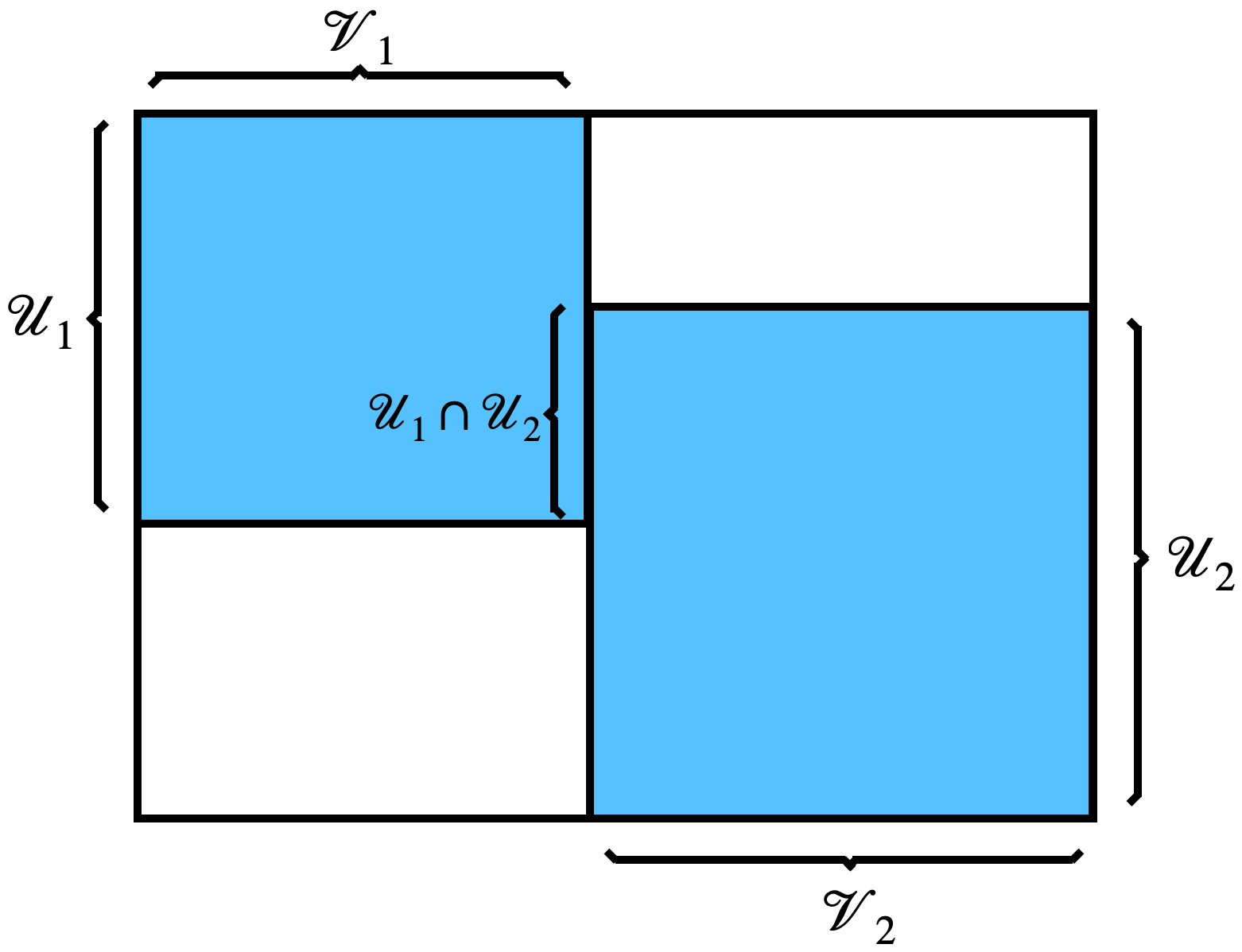
Figure 11: Submatrices with overlapping row indices but no overlapping entries.

Finally, we note that extending Theorem 4 to the asymmetric setting is also straightforward if we assume the entries of $\mathbf{N}^{(i)}$ are independent and that $|\mathcal{V}_{i}|\asymp|\mathcal{U}_{i}|$ for all $i$. Indeed, we can simply apply Theorem 4 to the Hermitean dilations of $\mathbf{A}^{(i)}$. However, the asymmetric case also allows for richer noise models such as the rows of $\mathbf{A}^{(i)}$ being independent but the entries in each row are dependent, or imbalanced dimensions where $|\mathcal{U}_{i}|\ll|\mathcal{V}_{i}|$ or vice versa for some indices $i$. We leave theoretical results for these more general settings to future work.

Supplementary Material for “Chain-lined Multiple Matrix Integration via Embedding Alignment”

Appendix A Discussion for Multiple Matrix Data Integration

If we are given a chain of overlapping submatrices of some larger matrix $\mathbf{P}$, then Algorithm 1 provides a simple and computationally efficient procedure for recovering the unobserved regions of $\mathbf{P}$. In practice, before applying Algorithm 1 we need to resolve two other crucial issues: 1) determining if a chain exists for a particular unobserved entry and 2) if there exists more than one feasible chain, how to select one chain or combine multiple chains. We discuss the recoverability of entries in Section A.1. In Section A.2 and Section A.3 we discuss the issue of chain selection for two cases: 1) we want to recover a specific unobserved entry; 2) integrating several block-wise overlapping noisy matrices. Finally in Section A.4 we discuss the use of a preprocessing step proposed in Zhou et al. (2023) to aggregate multiple observed values by introducing weights to each source. The algorithms are illustrated for positive semidefinite matrices, and it can be easily extended to the cases of symmetric indefinite matrices and asymmetric or rectangular matrices.

A.1 Determine the recoverability of entries

For a matrix of $N$ entities, suppose that we have $K$ observed submatrices associated with entities sets $\mathcal{U}_{1},\dots,\mathcal{U}_{K}$ from different sources. We then construct an undirected graph $\mathcal{G}$ to determine which unobserved entries can be recovered. More specifically, $\mathcal{G}$ has $K$ vertices $\{v_{1},\dots,v_{K}\}$ such that $v_{i}$ and $v_{j}$ are adjacent if and only if $\mathcal{U}_{i}$ and $\mathcal{U}_{j}$ are overlapping, i.e., $|\mathcal{U}_{i}\cap\mathcal{U}_{j}|\geq d$. For any unobserved entry $(s,t)$ in $\mathbf{P}$, we set $B^{(s)}:=\{i\mid s\in\mathcal{U}_{i}\}$ and $B^{(t)}:=\{j\mid t\in\mathcal{U}_{j}\}$. As long as there exist $i\in B^{(s)}$ and $j\in B^{(t)}$ such that $v_{i}$ and $v_{j}$ are connected in $\mathcal{G}$, we can estimate $\mathbf{P}_{s,t}$ by at least one chain of overlapping submatrices. Furthermore, the connected components of $\mathcal{G}$ also provide information on all recoverable entries. More specifically, suppose $\mathcal{G}$ has $F$ connected components, which can be found by depth-first search (DFS) efficiently. For each component $f\in[F]$, let $\mathcal{I}^{[f]}:=\{i|v_{i}\text{ is in the component }f\}$, and construct the entity set $\mathcal{U}^{[f]}:=\bigcup_{i\in\mathcal{I}^{[f]}}\mathcal{U}_{i}$ to contain all entities involved in this component. Then whenever $s$ and $t$ are both elements of $\mathcal{U}^{[f]}$ for some $f\in[F]$, the entry $(s,t)$ is recoverable using only the observed $\{\mathbf{A}^{(i)}\}_{i\in\mathcal{I}^{[f]}}$. See Algorithm 2 for details.

0:  Entities sets $\mathcal{U}_{1},\dots,\mathcal{U}_{K}\subset[N]$. 1. Let $\mathcal{G}$ have vertices $v_{1},\dots,v_{K}$; $v_{i}$ and $v_{j}$ are adjacent if and only if $|\mathcal{U}_{i}\cap\mathcal{U}_{j}|\geq d$. 2. Apply DFS to find the connected components of $\mathcal{G}$. Suppose there are $F$ connected components and the index set of each component $f\in[F]$ is denoted by $\mathcal{I}^{[f]}=\{i|v_{i}\text{ is in the component }f\}$. 3. For each component $f\in[F]$, define $\mathcal{U}^{[f]}=\underset{i\in\mathcal{I}^{[f]}}{\bigcup}\mathcal{U}_{i}.$ 4. Initialize $\mathbf{F}$ as a $N\times N$ matrix with all elements set to $0$, and for $f\in[F]$ do $\mathbf{F}_{\mathcal{U}^{[f]},\mathcal{U}^{[f]}}\leftarrow\bm{1}$ where $\bm{1}$ is a $|\mathcal{U}^{[f]}|\times|\mathcal{U}^{[f]}|$ matrix of all ones; end for 0:  Matrix $\mathbf{F}$ with $\mathbf{F}_{s,t}=1$ whenever $\mathbf{P}_{s,t}$ is recoverable.

Algorithm 2 Determining the recoverability of entries

A.2 Choosing among multiple chains

For any arbitrary unobserved entry $\mathbf{P}_{s,t}$, we can use the graph $\mathcal{G}$ described in Section A.1 to determine all feasible chains of overlapping submatrices for recovering $\mathbf{P}_{s,t}$; indeed, each path in $\mathcal{G}$ corresponds to one such chain. We now describe how our theoretical analysis in Section 3 can provide guidance for choosing a “good” chain. For ease of exposition, we will henceforth assume that $\mathcal{G}$ is connected and thus all entries that appeare in our matrix is recoverable. If $\mathcal{G}$ has more than one connected component then we can consider each connected component separately.

First recall that $\mathbf{E}^{({i_{0}})}\mathbf{X}_{\mathcal{U}_{i_{0}}}(\mathbf{X}_{\mathcal{U}_{i_{0}}}^{\top}\mathbf{X}_{\mathcal{U}_{i_{0}}})^{-1}\mathbf{X}_{\mathcal{U}_{i_{L}}}^{\top}+\mathbf{X}_{\mathcal{U}_{i_{0}}}(\mathbf{X}_{\mathcal{U}_{i_{L}}}^{\top}\mathbf{X}_{\mathcal{U}_{i_{L}}})^{-1}\mathbf{X}_{\mathcal{U}_{i_{L}}}^{\top}\mathbf{E}^{({i_{L}})}$ is the dominant error term in Theorem 2. And if the noise levels of $\mathbf{E}^{({i_{0}})}$ and $\mathbf{E}^{({i_{L}})}$ are homogenous then

$$\|\mathbf{E}^{({i_{0}})}\mathbf{X}_{\mathcal{U}_{i_{0}}}(\mathbf{X}_{\mathcal{U}_{i_{0}}}^{\top}\mathbf{X}_{\mathcal{U}_{i_{0}}})^{-1}\mathbf{X}_{\mathcal{U}_{i_{L}}}^{\top}\|_{\max}\lesssim\|\mathbf{E}^{(i_{0})}\|_{F}/n_{i_{0}}^{3/2}\cdot\log n_{i_{0}},$$ (A.1)

$$\|\mathbf{X}_{\mathcal{U}_{i_{0}}}(\mathbf{X}_{\mathcal{U}_{i_{L}}}^{\top}\mathbf{X}_{\mathcal{U}_{i_{L}}})^{-1}\mathbf{X}_{\mathcal{U}_{i_{L}}}^{\top}\mathbf{E}^{({i_{L}})}\|_{\max}\lesssim\|\mathbf{E}^{(i_{L})}\|_{F}/n_{i_{L}}^{3/2}\cdot\log n_{i_{L}}$$ (A.2)

with high probability. Note that the bounds on the right sides of Eq. (A.1) and Eq. (A.2) depend only on the first and last submatrices of the chain, respectively, and they can be estimated from the observed data. Indeed, $n_{i_{0}}$ and $n_{i_{L}}$ are given, while $\|\mathbf{E}^{(i_{0})}\|_{F}$ can be approximated by $\|\mathbf{A}^{(i_{0})}-\hat{\mathbf{U}}^{(i_{0})}\hat{\bm{\Lambda}}^{(i_{0})}\hat{\mathbf{U}}^{(i_{0})\top}\|_{F}$, with a similar approximation for $\|\mathbf{E}^{(i_{L})}\|_{F}$. We thus only need to specify the start and end points of a chain. Let

$$c_{i}=\|\mathbf{A}^{(i)}-\hat{\mathbf{U}}^{(i)}\hat{\bm{\Lambda}}^{(i)}\hat{\mathbf{U}}^{(i)\top}\|_{F}\cdot\log n_{i}/n_{i}^{3/2}$$ (A.3)

for any $i\in[K]$. Then for any arbitrary unobserved entry $(s,t)$, set

$$(i_{0},i_{L})=\underset{\begin{subarray}{c}(i,j)\in B^{(s)}\times B^{(t)}\end{subarray}}{\arg\min}(c_{i}+c_{j}).$$ (A.4)

As the influence of the middle nodes of the chain on the estimation error is negligible (see Theorem 2 ), for simplicity we set these nodes to form the shortest path between $v_{i_{0}}$ and $v_{i_{L}}$ in $\mathcal{G}$, which can be obtained by breadth-first search (BFS). See Algorithm 3 for details.

0:  Embedding dimension $d$, observed submatrices $\mathbf{A}^{(1)},\dots,\mathbf{A}^{(K)}$ for $\mathcal{U}_{1},\dots,\mathcal{U}_{K}\subset[N]$, the entry of interest $(s,t)\in[N]\times[N]$.   Step 1 Constructing the graph $\mathcal{G}$, the vertices sets $B^{(s)},B^{(t)}$ and $\{c_{i}\}_{i\in B^{(s)}\cup B^{(t)}}$: 1. $\mathcal{G}$ have $K$ vertices $v_{1},\dots,v_{K}$, and $v_{i},v_{j}$ are adjacent if and only if $|\mathcal{U}_{i}\cap\mathcal{U}_{j}|\geq d$. 2. Obtain vertices sets $B^{(s)}\leftarrow\{i\mid s\in\mathcal{U}_{i}\},\ B^{(t)}\leftarrow\{j\mid t\in\mathcal{U}_{j}\}.$ 3. For each $i\in B^{(s)}\cup B^{(t)}$, compute $c_{i}=\|\mathbf{A}^{(i)}-\hat{\mathbf{U}}^{(i)}\hat{\bm{\Lambda}}^{(i)}\hat{\mathbf{U}}^{(i)\top}\|_{F}\cdot\log|\mathcal{U}_{i}|/|\mathcal{U}_{i}|^{3/2}.$   Step 2 Finding the “good” feasible chain according to Eq. (A.4): Set $i_{0}\leftarrow\underset{i\in B^{(s)}}{\operatorname{argmin}}\ c_{i},\ i_{L}\leftarrow\underset{j\in B^{(t)}}{\operatorname{argmin}}\ c_{j}.$ Apply BFS to find the shortest path between $v_{i_{0}}$ and $v_{i_{L}}$ in $\mathcal{G}$, denoted as $(i_{0},i_{1},\dots,i_{L})$.   The path $(i_{0},i_{1},\dots,i_{L})$.

Algorithm 3 Finding a “good” chain for a specific unobserved entry

A.3 Algorithm for holistic recovery

Suppose we have observed submatrices $\mathbf{A}^{(1)},\mathbf{A}^{(2)},\dots,\mathbf{A}^{(K)}$ for $\mathcal{U}_{1},\mathcal{U}_{2},\dots,\mathcal{U}_{K}\subset[N]$ and want to integrate them. Given Algorithm 3 in Section A.2, a straightforward idea is to recover all unobserved entries one by one, but this involves a significant amount of redundant and repetitive calculations. We now describe an approach for simplifying these calculations.

Suppose we have a graph $\mathcal{G}$ as visualized in panel (a) of Figure 12. Recall that each vertex $v_{i}$ in $\mathcal{G}$ is associated with an observed submatrix $\mathbf{A}^{(i)}$ with estimated latent position matrix $\hat{\mathbf{X}}^{(i)}$. Furthermore, if $v_{i}$ and $v_{j}$ are adjacent in $\mathcal{G}$ then the corresponding submatrices $\mathbf{A}^{(i)}$ and $\mathbf{A}^{(j)}$ are overlapping and we can find an orthogonal matrix $\mathbf{W}^{(i,j)}$ to align $\hat{\mathbf{X}}^{(i)}$ and $\hat{\mathbf{X}}^{(j)}$. Note that $\mathcal{G}$ in panel (a) of Figure 12 has cycles, and thus there exists at least one pair of vertices $v_{k}$ and $v_{\ell}$ with multiple paths between them. We now want to find a unique path from every vertex to every other vertex, so that all the latent position matrices $\{\hat{\mathbf{X}}^{(i)}\}_{i\in[K]}$ can be aligned together and all the unobserved entries can be recovered simultaneously. This problem can be addressed using a spanning tree of $\mathcal{G}$; see panel (b) of Figure 12. Recall that $c_{i}$ defined in Eq. (A.3) reflects the magnitude of the error for $\mathbf{A}^{(i)}$ as an estimate of $\mathbf{P}^{(i)}$, and thus we want our tree to have paths passing through vertices with small estimation errors. This can be achieved by setting the weight of any edge $e_{ij}$ in $\mathcal{G}$ to $c_{i}+c_{j}$ and then finding the minimum spanning tree (MST) of $\mathcal{G}$; see panel (c) of Figure 12.

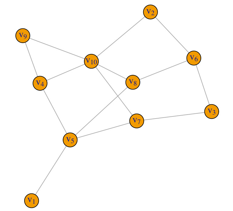
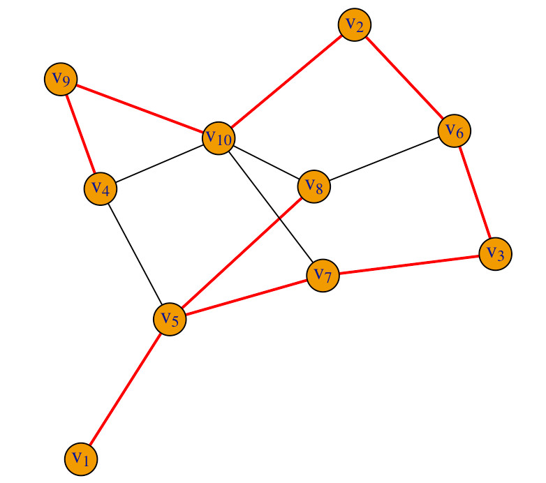
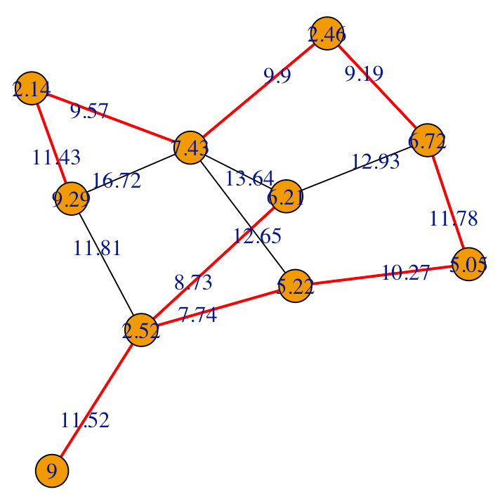
Figure 12: An example of a graph $\mathcal{G}$ described in Section A.3 (see panel (a)). Panel (b) gives a spanning tree of $\mathcal{G}$. In Panel (c), we suppose the vertices have the estimation error magnitudes $\{c_{i}\}$ as shown in the labels of vertices. The edges weights between vertices $i$ and $j$ are given by $c_{i}+c_{j}$, and we highlight the minimum spanning tree of $\mathcal{G}$ using red colored lines.

Given a minimum spanning tree, we choose a $i_{*}$ at random and align the remaining $\{\hat{\mathbf{X}}^{(i)}\}_{i\not=i_{*}}$ to $\hat{\mathbf{X}}^{(i_{*})}$ using the unique path. See Algorithm 4 for details.

0: Embedding dimension $d$, observed submatrices $\mathbf{A}^{(1)},\mathbf{A}^{(2)},\dots,\mathbf{A}^{(K)}$ for $\mathcal{U}_{1},\mathcal{U}_{2},\dots,\mathcal{U}_{K}\subset[N]$.

  Step 1 Constructing the weighted graph $\mathcal{G}$:

1. $\mathcal{G}$ have $K$ vertices $v_{1},\dots,v_{K}$, and $v_{i},v_{j}$ are adjacent if and only if $|\mathcal{U}_{i}\cap\mathcal{U}_{j}|\geq d$.

2. For each $i\in[K]$, compute $c_{i}=\|\mathbf{A}^{(i)}-\hat{\mathbf{U}}^{(i)}\hat{\bm{\Lambda}}^{(i)}\hat{\mathbf{U}}^{(i)\top}\|_{F}\cdot\log|\mathcal{U}_{i}|/|\mathcal{U}_{i}|^{3/2}$, and obtain estimated latent positions for $\mathcal{U}_{i}$, denoted by $\hat{\mathbf{X}}^{(i)}=\hat{\mathbf{U}}^{(i)}(\hat{\bm{\Lambda}}^{(i)})^{1/2}$.

3. Set the weight of each edge $e_{i,j}$ as $c_{i}+c_{j}$.

 Step 2 Obtaining the aligned latent position estimates $\{\tilde{\mathbf{X}}^{(i)}\}_{i\in[K]}$:

1. Find the minimum spanning tree of $\mathcal{G}$ by Prim’s algorithm or Kruskal’s algorithm, and denote its edge set by $E_{MST}$.

2. For each edge $e_{i,j}\in E_{MST}$, obtain $\mathbf{W}^{(i,j)}$ via the orthogonal Procrustes problem

   $$\mathbf{W}^{(i,j)}=\underset{\mathbf{O}\in\mathcal{O}_{d}}{\operatorname{argmin}}\|\hat{\mathbf{X}}^{(i)}_{\langle\mathcal{U}_{i}\cap\mathcal{U}_{j}\rangle}\mathbf{O}-\hat{\mathbf{X}}^{(j)}_{\langle\mathcal{U}_{i}\cap\mathcal{U}_{j}\rangle}\|_{F}.$$

3. Choose one of the vertex denoted by $v_{i^{\star}}$ (for example, $i^{\star}=1$), and let $\tilde{\mathbf{X}}^{(i^{\star})}=\hat{\mathbf{X}}^{(i^{\star})}$.

4. For each $i\in[K]\backslash\{i^{\star}\}$, apply BFS to find a path from $i$ to $i^{\star}$, denoted by $(i_{0}=i,i_{1},\dots,i_{L}=i^{\star})$, and let $\tilde{\mathbf{X}}^{(i)}=\hat{\mathbf{X}}^{(i)}\mathbf{W}^{(i_{0},i_{1})}\cdots\mathbf{W}^{(i_{L-1},i_{L})}$.

 Step 3 Obtaining the holistic latent position estimate $\tilde{\mathbf{X}}\in\mathbb{R}^{N\times d}$:

1. Sort $\{c_{i}\}_{i\in[K]}$ in descending order and record their indices as $(i_{1},i_{2},\dots,i_{K})$.

2. Initialize $\tilde{\mathbf{X}}$ as an ${N\times d}$ matrix, and

   for $i=i_{1}$ to $i_{K}$ do

   $\tilde{\mathbf{X}}_{\mathcal{U}_{i}}\leftarrow\tilde{\mathbf{X}}^{(i)}$;

   end for

 $\hat{\mathbf{P}}=\tilde{\mathbf{X}}\tilde{\mathbf{X}}^{\top}$.

Algorithm 4 Algorithm for holistic recovery

A.4 Aggregating multiple observed values for the same entry

Finally we note that as the same entry can appear in more than one observed submatrix, we can also apply a preprocessing step proposed in Zhou et al. (2023) to aggregate these multiple observed values. This preprocessing is especially useful when the observed submatrices have many overlapping regions as it can reduce the noise and proportion of missing observations for each submatrix. Let $(s,t)\in[N]\times[N]$ be arbitrary, and denote by $\mathcal{V}^{[s,t]}\subset[K]$ the set of matrices in which the $(s,t)$ entry appears. Zhou et al. (2023) show that one can weight each source $i\in\mathcal{V}^{[s,t]}$ by $\frac{1}{\sigma_{i}^{2}}$. As $\sigma_{i}^{2}$ is generally unknown, it can be estimated by $\hat{\sigma}_{i}^{2}=\|(\mathbf{B}^{(i)}-\hat{\mathbf{P}}^{(i)})\circ\mathbf{\Omega}^{(i)}\|_{F}^{2}/\|\bm{\Omega}^{(i)}\|_{F}^{2}$. Here $\mathbf{B}^{(i)}=(\mathbf{P}^{(i)}+\mathbf{N}^{(i)})\circ\mathbf{\Omega}^{(i)}$ is the observed matrix, and $\hat{\mathbf{P}}^{(i)}=\hat{\mathbf{U}}^{(i)}\hat{\bm{\Lambda}}^{(i)}\hat{\mathbf{U}}^{(i)\top}$ is the rank-$d$ eigendecomposition of $\mathbf{B}^{(i)}/q_{i}$. Given $\{\hat{\sigma}^{2}_{i}\}$, the aggregated observed value for $(s,t)$ is then set to

$$\sum_{i\in\mathcal{V}^{[s,t]}}\alpha^{[s,t]}_{i}\mathbf{B}^{(i)}_{\langle s,t\rangle},\quad\text{where}\quad\alpha^{[s,t]}_{i}=\big{(}\sum_{j\in\mathcal{V}^{[s,t]}}\frac{1}{\hat{\sigma}_{j}^{2}}\big{)}^{-1}\cdot\frac{1}{\hat{\sigma}_{i}^{2}}.$$

Here $\mathbf{B}^{(i)}_{\langle s,t\rangle}$ is the value for the $(s,t)$ entry in $\mathbf{B}^{(i)}$ and $\{\alpha_{i}^{[s,t]}\}_{i\in\mathcal{V}^{[s,t]}}$ are the normalized weights.

$$\alpha^{[s,t]}_{i}=\big{(}\sum_{j\in\mathcal{V}^{[s,t]}}\frac{1}{\hat{\sigma}_{j}^{2}}\big{)}^{-1}\cdot\frac{1}{\hat{\sigma}_{i}^{2}}.$$

See Algorithm 5 for details.

0: Embedding dimension $d$, observed submatrices $\{\mathbf{B}^{(i)}\}_{i\in[K]}$ for $\{\mathcal{U}_{i}\}_{i\in[K]}$ with $\{\mathbf{\Omega}^{(i)}\}_{i\in[K]}$ indicating observed entries. Here $\{\mathbf{B}^{(i)}\}_{i\in[K]}$ is defined as described in Section A.4.

  Step 1 Obtaining the aggregated observed matrix $\tilde{\mathbf{B}}\in\mathbb{R}^{N\times N}$:

1. For each $i\in[K]$, estimate $\sigma^{2}$ by

   $$\hat{\sigma}_{i}^{2}=\|(\mathbf{B}^{(i)}-\hat{\mathbf{U}}^{(i)}\hat{\bm{\Lambda}}^{(i)}\hat{\mathbf{U}}^{(i)\top})\circ\mathbf{\Omega}^{(i)}\|_{F}^{2}/\|\bm{\Omega}^{(i)}\|_{F}^{2},$$

   where $\hat{\mathbf{U}}^{(i)}\hat{\bm{\Lambda}}^{(i)}\hat{\mathbf{U}}^{(i)\top}$ is the rank-$d$ eigendecomposition of $\mathbf{B}^{(i)}/q_{i}$ with $q_{i}=\|\bm{\Omega}^{(i)}\|_{F}^{2}/|\mathcal{U}_{i}|^{2}$.

2. Initialize $\tilde{\mathbf{B}}\leftarrow\mathbf{0}^{N\times N},\tilde{\mathbf{\Omega}}\leftarrow\mathbf{0}^{N\times N}$.

   For each $(s,t)\in[N]\times[N]$, set $\mathcal{V}^{[s,t]}=\{i\mid\mathbf{\Omega}^{(i)}_{\langle s,t\rangle}=1\}$.

   if $|\mathcal{V}^{[s,t]}|\geq 1$ then

   Compute $S=\sum_{j\in\mathcal{V}^{[s,t]}}\hat{\sigma}_{j}^{-2}$.

   Set $\alpha^{[s,t]}_{i}=\hat{\sigma_{i}}^{-2}S^{-1}$ for each $i\in\mathcal{V}^{[s,t]}$.

   Set $\tilde{\mathbf{B}}_{s,t}\leftarrow\sum_{i\in\mathcal{V}^{[s,t]}}\alpha^{[s,t]}_{i}\mathbf{B}^{(i)}_{\langle s,t\rangle}$ and $\tilde{\mathbf{\Omega}}_{s,t}\leftarrow 1$.

   end if

 Step 2 Obtaining the preprocessed observed matrices $\{\mathbf{A}^{(i)}\}_{i\in[K]}$:

1. For each $i\in[K]$, set $\tilde{\mathbf{B}}^{(i)}\leftarrow\tilde{\mathbf{B}}_{\mathcal{U}_{i},\mathcal{U}_{i}}$ and $\tilde{\mathbf{\Omega}}^{(i)}\leftarrow\tilde{\mathbf{\Omega}}_{\mathcal{U}_{i},\mathcal{U}_{i}}$.

2. Estimate $q_{i}$ by $\hat{q}_{i}=\|\tilde{\mathbf{\Omega}}^{(i)}\|_{F}^{2}/|\mathcal{U}_{i}|^{2}$ and set $\mathbf{A}^{(i)}=\tilde{\mathbf{B}}^{(i)}/\hat{q}_{i}$.

 The preprocessed observed matrices $\{\mathbf{A}^{(i)}\}_{i\in[K]}$.

Algorithm 5 Aggregating multiple observed values for the same entry

Appendix B Algorithms and Simulation Results for Section 6

B.1 Symmetric indefinite matrices integration

0: Embedding dimensions $d_{+}$ and $d_{-}$ for positive and negative eigenvalues, respectively; a chain of overlapping submatrices $\mathbf{A}^{(0)},\mathbf{A}^{(i_{1})},\dots,\mathbf{A}^{(i_{L})}$ for $\mathcal{U}_{i_{0}},\mathcal{U}_{i_{1}},\dots,\mathcal{U}_{i_{L}}$ with $\min\{|\mathcal{U}_{i_{0}}\cap\mathcal{U}_{i_{1}}|,|\mathcal{U}_{i_{1}}\cap\mathcal{U}_{i_{2}}|,\dots,|\mathcal{U}_{i_{L-1}}\cap\mathcal{U}_{i_{L}}|\}\geq d$.

1. For each $0\leq\ell\leq L$, obtain the estimated latent positions $\hat{\mathbf{X}}^{(i_{\ell})}=\hat{\mathbf{U}}^{(i_{\ell})}|\hat{\bm{\Lambda}}^{(i_{\ell})}|^{1/2}$.

2. For each $1\leq\ell\leq L$, obtain $\mathbf{W}^{(i_{\ell-1},i_{\ell})}$ by solving the least square optimization problem

   $$\mathbf{W}^{(i_{\ell-1},i_{\ell})} =\underset{\mathbf{O}\in\mathbb{R}^{d\times d}}{\operatorname{argmin}}\|\hat{\mathbf{X}}^{(i_{\ell-1})}_{\langle\mathcal{U}_{i_{\ell-1}}\cap\mathcal{U}_{i_{\ell}}\rangle}\mathbf{O}-\hat{\mathbf{X}}^{(i_{\ell})}_{\langle\mathcal{U}_{i_{\ell-1}}\cap\mathcal{U}_{i_{\ell}}\rangle}\|_{F}.$$

3. Compute $\hat{\mathbf{P}}_{\mathcal{U}_{i_{0}},\mathcal{U}_{i_{L}}}=\hat{\mathbf{X}}^{(i_{0})}\mathbf{W}^{(i_{0},i_{1})}\mathbf{W}^{(i_{1},i_{2})}\cdots\mathbf{W}^{(i_{L}-1,i_{L})}\mathbf{I}_{d_{+},d_{-}}\hat{\mathbf{X}}^{(i_{L})\top}$.

0: $\hat{\mathbf{P}}_{\mathcal{U}_{i_{0}},\mathcal{U}_{i_{L}}}$.

Algorithm 6 CMMI for overlapping submatrices of a symmetric indefinite matrix

We compare the performance of Algorithm 6 with other matrix completion methods. Consider the setting of Section 4.2, but with $\bm{\Lambda}=\mathrm{diag}(N,\tfrac{1}{2}N,-\tfrac{1}{2}N,-N)$, and thus $d_{+}=d_{-}=2$. Figure 13 shows the relative $F$-norm estimation error results for CMMI against other matrix completion algorithms.

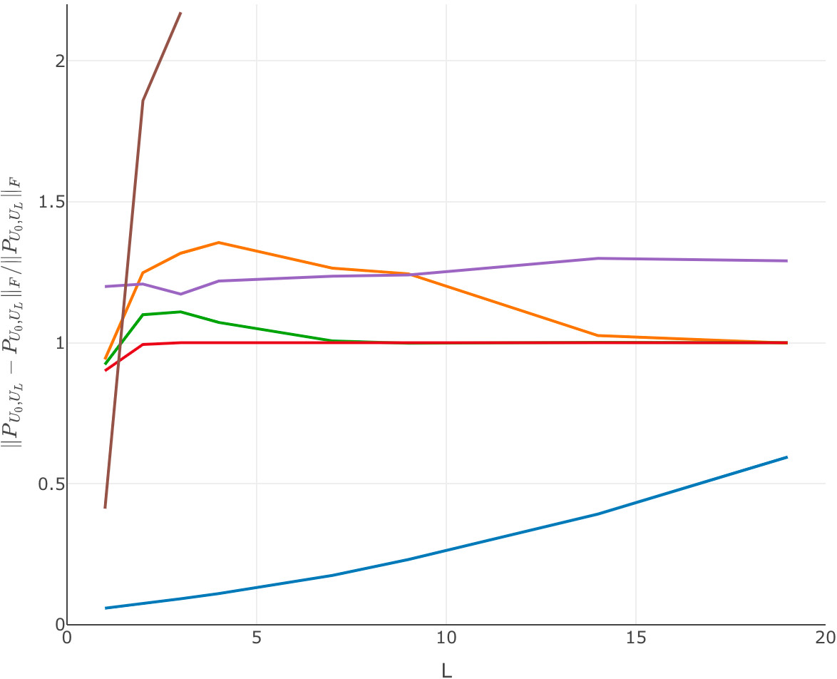
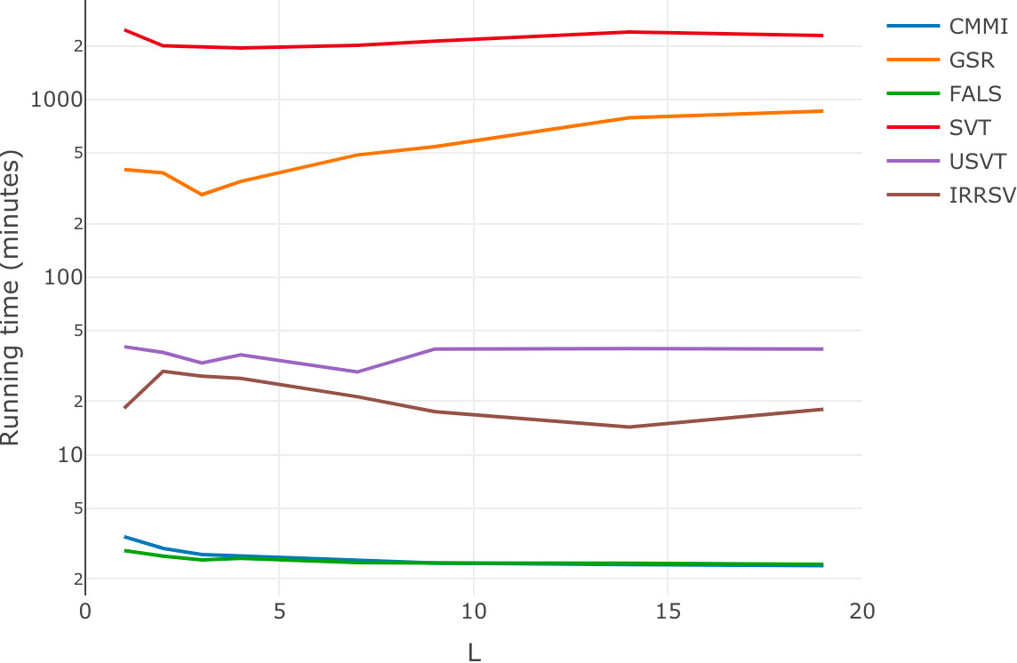
Figure 13: The left panel reports relative $F$-norm errors $\|\hat{\mathbf{P}}_{\mathcal{U}_{0},\mathcal{U}_{L}}-\mathbf{P}_{\mathcal{U}_{0},\mathcal{U}_{L}}\|_{F}/\|\mathbf{P}_{\mathcal{U}_{0},\mathcal{U}_{L}}\|_{F}$ for CMMI and other low-rank matrix completion algorithms as $L$ changes. In particular, we vary $L=\{1,2,3,4,7,9,14,19\}$ while fixing $N\approx 2200$, $\breve{p}=0.1$, $q=0.8$, $\sigma=0.5$. The results are averaged over $100$ independent Monte Carlo replicates. Note that the averaged relative $F$-norm errors of IRRSV are $\{0.4,1.9,2.2,3.5,20.5,36.8,331.7,1865.6\}$ and a portion of these errors are too large to be displayed together with the errors of other algorithms, so we ignore the excessively large values in the left panel. The right panel reports running time for all algorithms and different $L$. For each setting we run $100$ independent Monte Carlo replicates with 10-core parallel computing.

B.2 Asymmetric matrices integration

0: Embedding dimension $d$, a chain of overlapping submatrices $\mathbf{A}^{(i_{0})},\mathbf{A}^{(i_{1})},\dots,\mathbf{A}^{(i_{L})}$ for $(\mathcal{U}_{i_{0}},\mathcal{V}_{i_{0}}),(\mathcal{U}_{i_{1}},\mathcal{V}_{i_{1}}),\dots,(\mathcal{U}_{i_{L}},\mathcal{V}_{i_{L}})$; here for each $\ell\in[L]$, we have $|\mathcal{U}_{i_{\ell-1}}\cap\mathcal{U}_{i_{\ell}}|\geq d$ or $|\mathcal{V}_{i_{\ell-1}}\cap\mathcal{V}_{i_{\ell}}|\geq d$.

1. For each $0\leq\ell\leq L$, obtain estimated left latent positions for $\mathcal{U}_{i_{\ell}}$ as $\hat{\mathbf{X}}^{(i_{\ell})}=\hat{\mathbf{U}}^{(i_{\ell})}(\hat{\bm{\Sigma}}^{(i_{\ell})})^{1/2}$ and right latent positions for $\mathcal{V}_{i_{\ell}}$ as $\hat{\mathbf{Y}}^{(i_{\ell})}=\hat{\mathbf{V}}^{(i_{\ell})}(\hat{\bm{\Sigma}}^{(i_{\ell})})^{1/2}$.

2. For each $1\leq\ell\leq L$, obtain $\mathbf{W}^{(i_{\ell-1},i_{\ell})}$:

   if $|\mathcal{U}_{i_{\ell-1}}\cap\mathcal{U}_{i_{\ell}}|\geq d$ and $|\mathcal{V}_{i_{\ell-1}}\cap\mathcal{V}_{i_{\ell}}|\geq d$ then

   Compute $\mathbf{W}^{(i_{\ell-1},i_{\ell})}=\frac{1}{2}(\mathbf{W}_{\mathbf{X}}^{(i_{\ell-1},i_{\ell})}+\mathbf{W}_{\mathbf{Y}}^{(i_{\ell-1},i_{\ell})})$ where

   $$\mathbf{W}_{\mathbf{X}}^{(i_{\ell-1},i_{\ell})} =\underset{\mathbf{O}\in\mathbb{R}^{d\times d}}{\operatorname{argmin}}\|\hat{\mathbf{X}}^{(i_{\ell-1})}_{\langle\mathcal{U}_{i_{\ell-1}}\cap\mathcal{U}_{i_{\ell}}\rangle}\mathbf{O}-\hat{\mathbf{X}}^{(i_{\ell})}_{\langle\mathcal{U}_{i_{\ell-1}}\cap\mathcal{U}_{i_{\ell}}\rangle}\|_{F},$$

   $$\mathbf{W}_{\mathbf{Y}}^{(i_{\ell-1},i_{\ell})\top} =\underset{\mathbf{O}\in\mathbb{R}^{d\times d}}{\operatorname{argmin}}\|\hat{\mathbf{Y}}^{(i_{\ell})}_{\langle\mathcal{V}_{i_{\ell-1}}\cap\mathcal{V}_{i_{\ell}}\rangle}\mathbf{O}-\hat{\mathbf{Y}}^{(i_{\ell-1})}_{\langle\mathcal{V}_{i_{\ell-1}}\cap\mathcal{V}_{i_{\ell}}\rangle}\|_{F}.$$

   else if $|\mathcal{U}_{i_{\ell-1}}\cap\mathcal{U}_{i_{\ell}}|\geq d$ then

   Compute $\begin{aligned} \mathbf{W}^{(i_{\ell-1},i_{\ell})}&=\underset{\mathbf{O}\in\mathbb{R}^{d\times d}}{\operatorname{argmin}}\|\hat{\mathbf{X}}^{(i_{\ell-1})}_{\langle\mathcal{U}_{i_{\ell-1}}\cap\mathcal{U}_{i_{\ell}}\rangle}\mathbf{O}-\hat{\mathbf{X}}^{(i_{\ell})}_{\langle\mathcal{U}_{i_{\ell-1}}\cap\mathcal{U}_{i_{\ell}}\rangle}\|_{F}.\end{aligned}$

   else

   Compute $\mathbf{W}^{(i_{\ell-1},i_{\ell})}$ by $\begin{aligned} \mathbf{W}^{(i_{\ell-1},i_{\ell})\top}&=\underset{\mathbf{O}\in\mathbb{R}^{d\times d}}{\operatorname{argmin}}\|\hat{\mathbf{Y}}^{(i_{\ell})}_{\langle\mathcal{V}_{i_{\ell-1}}\cap\mathcal{V}_{i_{\ell}}\rangle}\mathbf{O}-\hat{\mathbf{Y}}^{(i_{\ell-1})}_{\langle\mathcal{V}_{i_{\ell-1}}\cap\mathcal{V}_{i_{\ell}}\rangle}\|_{F}.\end{aligned}$

   end if

3. Compute $\hat{\mathbf{P}}_{\mathcal{U}_{i_{0}},\mathcal{V}_{i_{L}}}=\hat{\mathbf{X}}^{(i_{0})}\mathbf{W}^{(i_{0},i_{1})}\mathbf{W}^{(i_{1},i_{2})}\cdots\mathbf{W}^{(i_{L}-1,i_{L})}\hat{\mathbf{Y}}^{(i_{L})\top}$.

0: $\hat{\mathbf{P}}_{\mathcal{U}_{i_{0}},\mathcal{V}_{i_{L}}}$.

Algorithm 7 CMMI for overlapping submatrices of an asymmetric matrix

We compare the performance of Algorithm 7 with other matrix completion methods. We simulate a chain of $(L+1)$ overlapping observed submatrices $\{\mathbf{A}^{(i)}\}_{i=0}^{L}$ for the underlying population matrix $\mathbf{P}$ as described in Figure 14, and then predict the yellow unknown block by Algorithm 7. We let all observed submatrices have the same dimension $n\times m$, and let all overlapping parts have the same dimension $(\breve{p}_{n}n)\times(\breve{p}_{m}m)$. For the observed submatrices, we generate the noise matrices $\{\mathbf{N}^{(i)}\}$ by $\mathbf{N}^{(i)}_{st}\stackrel{{\scriptstyle iid}}{{\sim}}\mathcal{N}(0,\sigma^{2})$ for all $i=0,1,\dots,L$ and all $s\in[n],t\in[m]$, and we let all observed submatrices have the same non-missing probability $q$. For the low-rank underlying population matrix $\mathbf{P}=\mathbf{U}\bm{\Sigma}\mathbf{V}^{\top}$, we randomly generate $\mathbf{U}$ and $\mathbf{V}$ from $\{\mathbf{O}\in\mathbb{R}^{N\times d}\mid\mathbf{O}^{\top}\mathbf{O}=\mathbf{I}\}$ and $\{\mathbf{O}\in\mathbb{R}^{M\times d}\mid\mathbf{O}^{\top}\mathbf{O}=\mathbf{I}\}$, respectively. We fix the rank as $d=3$, and set $\bm{\Sigma}=\text{diag}(N,\tfrac{3}{4}N,\tfrac{1}{2}N)$. We fix the dimensions of the entire matrix at $N\approx 2200$ and $M\approx 2800$, and we vary $L$, the length of the chain, while ensuring that the observed submatrices fully span the diagonal of the matrix Recall that as $L$ increases, we have more observed submarices but each observed submatrix is of smaller dimensions, which then increases the difficulty of recovering the original matrix $\mathbf{P}$. Figure 15 shows the relative $F$-norm estimation error results of recovering the yellow region.

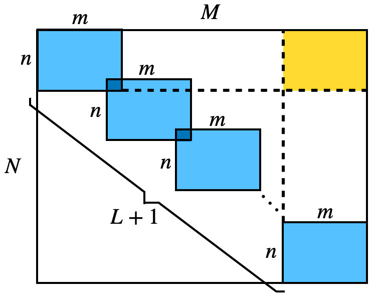
Figure 14: Simulation setting for an asymmetric matrix

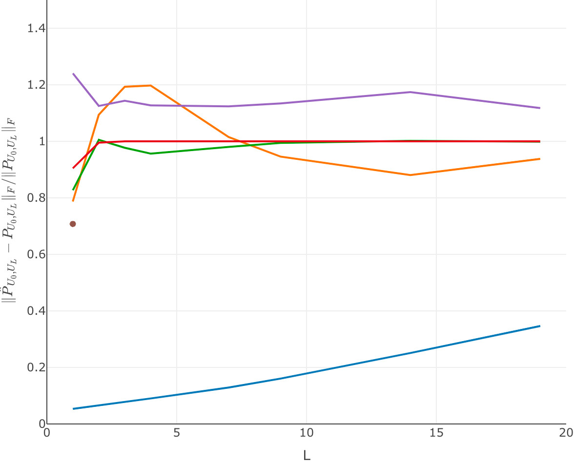
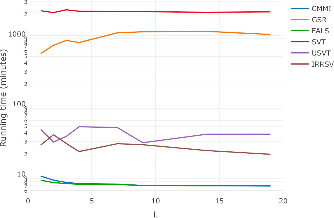
Figure 15: The left panel reports relative $F$-norm errors $\|\hat{\mathbf{P}}_{\mathcal{U}_{0},\mathcal{U}_{L}}-\mathbf{P}_{\mathcal{U}_{0},\mathcal{U}_{L}}\|_{F}/\|\mathbf{P}_{\mathcal{U}_{0},\mathcal{U}_{L}}\|_{F}$ for CMMI and other low-rank matrix completion algorithms as $L$ changes. In particular, we vary $L\in\{1,2,3,4,7,9,14,19\}$ while fixing $N\approx 2200$, $M\approx 2800$, $\breve{p}_{n}=\breve{p}_{m}=0.1$, $q=0.8$, $\sigma=0.5$. The results are averaged over $100$ independent Monte Carlo replicates. Note that the averaged relative $F$-norm errors of IRRSV are $\{0.7,8.0,26.1,28.2,26.4,42.9,79.3,211.1\}$ and a portion of these errors are too large to be displayed together with the errors of other algorithms, so we ignore the excessively large part in the left panel. The right panel reports running time for all algorithms and different $L$. For each setting we run $100$ independent Monte Carlo replicates with 10-core parallel computing.

Appendix C Proof of Main Results

C.1 Proof of Theorem 1

We first state two important technical lemmas, one for the error of $\hat{\mathbf{X}}^{(i)}$ as an estimate of the true latent position matrix $\mathbf{X}_{\mathcal{U}_{i}}$ for each $i\in[K]$, and another for the difference between $\mathbf{W}^{(i,j)}$ and $\mathbf{W}^{(i)}\mathbf{W}^{(j)\top}$. The proofs of these lemmas are presented in Section D.2 and Section D.5.

Lemma C.1.

Fix an $i\in[K]$ and consider $\mathbf{A}^{(i)}=(\mathbf{P}^{(i)}+\mathbf{N}^{(i)})\circ\mathbf{\Omega}^{(i)}/q_{i}\in\mathbb{R}^{n_{i}\times n_{i}}$ as defined in Eq. (2.1). Write the eigen-decompositions of $\mathbf{P}^{(i)}$ and $\mathbf{A}^{(i)}$ as

$$\mathbf{P}^{(i)}=\mathbf{U}^{(i)}\bm{\Lambda}^{(i)}\mathbf{U}^{(i)\top},\quad\mathbf{A}^{(i)}=\hat{\mathbf{U}}^{(i)}\hat{\bm{\Lambda}}^{(i)}\hat{\mathbf{U}}^{(i)\top}+\hat{\mathbf{U}}^{(i)}_{\perp}\hat{\bm{\Lambda}}^{(i)}_{\perp}\hat{\mathbf{U}}^{(i)\top}_{\perp}.$$

Let $\hat{\mathbf{X}}^{(i)}=\hat{\mathbf{U}}^{(i)}(\hat{\bm{\Lambda}}^{(i)})^{1/2}$. Next define $\mathbf{W}^{(i)}$ as a minimizer of $\|\hat{\mathbf{X}}^{(i)}\mathbf{O}-\mathbf{X}^{(i)}\|_{F}$ over all $d\times d$ orthogonal matrices $\mathbf{O}$. Suppose that

• $\mathbf{U}^{(i)}$ is a $n_{i}\times d$ matrix with bounded coherence, i.e.,

  $$\|\mathbf{U}^{(i)}\|_{2\to\infty}\lesssim d^{1/2}n_{i}^{-1/2}.$$

• $\mathbf{P}^{(i)}$ has bounded condition number, i.e.,

  $$\frac{\lambda_{i,\max}}{\lambda_{i,\min}}\leq M$$

  for some finite constant $M>0$; here $\lambda_{i,\max}$ and $\lambda_{i,\min}$ denote the largest and smallest non-zero eigenvalues of $\mathbf{P}^{(i)}$, respectively.

• The following conditions are satisfied.

  $$q_{i}n_{i}\gtrsim\log^{2}{n_{i}},\quad\frac{(\|\mathbf{P}^{(i)}\|_{\max}+\sigma_{i})n_{i}^{1/2}}{q_{i}^{1/2}\lambda_{i,\min}}=\frac{\gamma_{i}}{(q_{i}n_{i})^{1/2}\mu_{i}\log^{1/2}n_{i}}\ll 1.$$ (C.1)

We then have

$$\hat{\mathbf{X}}^{(i)}\mathbf{W}^{(i)}-\mathbf{X}_{\mathcal{U}_{i}}=\mathbf{E}^{(i)}\mathbf{X}_{\mathcal{U}_{i}}(\mathbf{X}_{\mathcal{U}_{i}}^{\top}\mathbf{X}_{\mathcal{U}_{i}})^{-1}+\mathbf{R}^{(i)},$$ (C.2)

where the remainder term $\mathbf{R}^{(i)}$ satisfies

$$\|\mathbf{R}^{(i)}\|\lesssim\frac{(\|\mathbf{P}^{(i)}\|_{\max}+\sigma_{i})^{2}n_{i}}{q_{i}\lambda_{i,\min}^{3/2}}+\frac{(\|\mathbf{P}^{(i)}\|_{\max}+\sigma_{i})\log^{1/2}n_{i}}{q_{i}^{1/2}\lambda_{i,\min}^{1/2}}$$

with high probability. If we further assume

$$\frac{(\|\mathbf{P}^{(i)}\|_{\max}+\sigma_{i})n_{i}^{1/2}\log^{1/2}n_{i}}{q_{i}^{1/2}\lambda_{i,\min}}=\frac{\gamma_{i}}{(q_{i}n_{i})^{1/2}\mu_{i}}\ll 1,$$ (C.3)

then we also have

$$\|\mathbf{R}^{(i)}\|_{2\to\infty}\lesssim\frac{(\|\mathbf{P}^{(i)}\|_{\max}+\sigma_{i})^{2}n_{i}^{1/2}\log n_{i}}{q_{i}\lambda_{i,\min}^{3/2}}+\frac{(\|\mathbf{P}^{(i)}\|_{\max}+\sigma_{i})\log^{1/2}n_{i}}{q_{i}^{1/2}n_{i}^{1/2}\lambda_{i,\min}^{1/2}}=\frac{\gamma_{i}^{2}}{q_{i}n_{i}\mu_{i}^{3/2}}+\frac{\gamma_{i}}{q_{i}^{1/2}n_{i}\mu_{i}^{1/2}},$$

$$\|\hat{\mathbf{X}}^{(i)}\mathbf{W}^{(i)}-\mathbf{X}_{\mathcal{U}_{i}}\|_{2\to\infty}\lesssim\|\mathbf{E}^{(i)}\mathbf{U}^{(i)}\|_{2\to\infty}\cdot\|(\bm{\Lambda}^{(i)})^{-1/2}\|+\|\mathbf{R}^{(i)}\|_{2\to\infty}$$

$$\quad\quad\quad\quad\quad\quad\quad\quad\quad\quad\lesssim\frac{(\|\mathbf{P}^{(i)}\|_{\max}+\sigma_{i})\log^{1/2}n_{i}}{q_{i}^{1/2}\lambda_{i,\min}^{1/2}}=\frac{\gamma_{i}}{(q_{i}n_{i}\mu_{i})^{1/2}}$$

with high probability.

Remark 7.

As $\mathbf{P}^{(i)}\in\mathbb{R}^{n_{i}\times n_{i}}$, we generally have $\|\mathbf{P}^{(i)}\|_{F}=\Theta(n_{i})$, e.g., $\mathbf{P}^{(i)}$ has $\Theta(n_{i}^{2})$ entries that are lower bounded by some constant $c_{0}$ not depending on $N$ or $n_{i}$. Thus, as $\mathbf{P}^{(i)}$ is low-rank with bounded condition number, we also have $\lambda_{i,\min}=\Theta(n_{i})$ and the second condition in Eq. (C.1) simplifies to

$$\frac{\|\mathbf{P}^{(i)}\|_{\max}+\sigma_{i}}{(q_{i}n_{i})^{1/2}}\ll 1.$$

Similarly, the condition in Eq. (C.3) simplifies to

$$\frac{(\|\mathbf{P}^{(i)}\|_{\max}+\sigma_{i})\log^{1/2}{n_{i}}}{(q_{i}n_{i})^{1/2}}\ll 1.$$

Both conditions are then trivially satisfied whenever $q_{i}n_{i}\gg\log{n_{i}}$ and $\|\mathbf{P}^{(i)}\|_{\max}+\sigma_{i}=O(1)$. Finally when $\lambda_{i,\min}=\Theta(n_{i})$, the bounds in Lemma C.1 simplify to

$$\|\mathbf{R}^{(i)}\|\lesssim\frac{(\|\mathbf{P}^{(i)}\|_{\max}+\sigma_{i})^{2}}{q_{i}n_{i}^{1/2}}+\frac{(\|\mathbf{P}^{(i)}\|_{\max}+\sigma_{i})\log^{1/2}{n_{i}}}{(q_{i}n_{i})^{1/2}},$$

$$\|\mathbf{R}^{(i)}\|_{2\to\infty}\lesssim\frac{(\|\mathbf{P}^{(i)}\|_{\max}+\sigma_{i})^{2}\log n_{i}}{q_{i}n_{i}}+\frac{(\|\mathbf{P}^{(i)}\|_{\max}+\sigma_{i})\log^{1/2}n_{i}}{q_{i}^{1/2}n_{i}},$$

$$\|\hat{\mathbf{X}}^{(i)}\mathbf{W}^{(i)}-\mathbf{X}_{\mathcal{U}_{i}}\|_{2\to\infty}\lesssim\frac{(\|\mathbf{P}^{(i)}\|_{\max}+\sigma_{i})\log^{1/2}n_{i}}{(q_{i}n_{i})^{1/2}}$$

with high probability.

Lemma C.2.

Consider the setting of Theorem 1. We then have

$$\|\mathbf{W}^{(i)\top}\mathbf{W}^{(i,j)}\mathbf{W}^{(j)}-\mathbf{I}\| \lesssim\frac{n_{i,j}\gamma_{i}\gamma_{j}}{\theta_{i,j}(q_{i}n_{i}\mu_{i})^{1/2}(q_{j}n_{j}\mu_{j})^{1/2}}+\frac{n_{i,j}^{1/2}\|\mathbf{X}_{\mathcal{U}_{i}\cap\mathcal{U}_{j}}\|_{2\to\infty}}{\theta_{i,j}}\Big{(}\frac{\gamma_{i}}{(q_{i}n_{i}\mu_{i})^{1/2}}+\frac{\gamma_{j}}{(q_{j}n_{j}\mu_{j})^{1/2}}\Big{)}$$

$$+\frac{(n_{i,j}\vartheta_{i,j})^{1/2}}{\theta_{i,j}}\Big{(}\frac{\gamma_{i}^{2}}{q_{i}n_{i}\mu_{i}^{3/2}}+\frac{\gamma_{j}^{2}}{q_{j}n_{j}\mu_{j}^{3/2}}\Big{)}=:\alpha_{i,j}$$

with high probability.

We now proceed with the proof of Theorem 1. Recall Eq. (C.2) and let $\xi_{i}:=\hat{\mathbf{X}}^{(i)}\mathbf{W}^{(i)}-\mathbf{X}^{(i)}$ for any $i$. Also denote $\tilde{\mathbf{W}}^{(i,j)}=\mathbf{W}^{(i)\top}\mathbf{W}^{(i,j)}\mathbf{W}^{(j)}$. We then have

$$\hat{\mathbf{X}}^{(i)}\mathbf{W}^{(i,j)}\hat{\mathbf{X}}^{(j)\top}-\mathbf{X}_{\mathcal{U}_{i}}\mathbf{X}_{\mathcal{U}_{j}}^{\top}= (\hat{\mathbf{X}}^{(i)}\mathbf{W}^{(i)})(\mathbf{W}^{(i)\top}\mathbf{W}^{(i,j)}\mathbf{W}^{(j)})(\mathbf{W}^{(j)\top}\hat{\mathbf{X}}^{(j)\top})-\mathbf{X}_{\mathcal{U}_{i}}\mathbf{X}_{\mathcal{U}_{j}}^{\top}$$

$$= (\mathbf{X}_{\mathcal{U}_{i}}+\xi_{i})\tilde{\mathbf{W}}^{(i,j)}(\mathbf{X}_{\mathcal{U}_{j}}+\xi_{j})^{\top}-\mathbf{X}_{\mathcal{U}_{i}}\mathbf{X}_{\mathcal{U}_{j}}^{\top}$$

$$= (\mathbf{X}_{\mathcal{U}_{i}}+\xi_{i})(\tilde{\mathbf{W}}^{(i,j)}-\mathbf{I})(\mathbf{X}_{\mathcal{U}_{j}}+\xi_{j})^{\top}+(\mathbf{X}_{\mathcal{U}_{i}}+\xi_{i})(\mathbf{X}_{\mathcal{U}_{j}}+\xi_{j})^{\top}-\mathbf{X}_{\mathcal{U}_{i}}\mathbf{X}_{\mathcal{U}_{j}}^{\top}$$

$$= \xi_{i}\mathbf{X}_{\mathcal{U}_{j}}^{\top}+\mathbf{X}_{\mathcal{U}_{i}}\xi_{j}^{\top}+\xi_{i}\xi_{j}^{\top}+(\mathbf{X}_{\mathcal{U}_{i}}+\xi_{i})(\tilde{\mathbf{W}}^{(i,j)}-\mathbf{I})(\mathbf{X}_{\mathcal{U}_{j}}+\xi_{j})^{\top}$$

$$= \mathbf{E}^{(i)}\mathbf{X}_{\mathcal{U}_{i}}(\mathbf{X}_{\mathcal{U}_{i}}^{\top}\mathbf{X}_{\mathcal{U}_{i}})^{-1}\mathbf{X}_{\mathcal{U}_{j}}^{\top}+\mathbf{X}_{\mathcal{U}_{i}}(\mathbf{X}_{\mathcal{U}_{j}}^{\top}\mathbf{X}_{\mathcal{U}_{j}})^{-1}\mathbf{X}_{\mathcal{U}_{j}}^{\top}\mathbf{E}^{(j)}+\mathbf{R}^{(i,j)}+\mathbf{S}^{(i,j)},$$

where we set

$$\mathbf{R}^{(i,j)}:=\mathbf{R}^{(i)}\mathbf{X}_{\mathcal{U}_{j}}^{\top}+\mathbf{X}_{\mathcal{U}_{i}}\mathbf{R}^{(j)\top}+\xi_{i}\xi_{j}^{\top},\quad\mathbf{S}^{(i,j)}:=(\mathbf{X}_{\mathcal{U}_{i}}+\xi_{i})(\tilde{\mathbf{W}}^{(i,j)}-\mathbf{I})(\mathbf{X}_{\mathcal{U}_{j}}+\xi_{j})^{\top}.$$ (C.4)

We now bound $\mathbf{R}^{(i,j)}$ and $\mathbf{S}^{(i,j)}$. Note that, for matrices $\mathbf{M}_{1}$ and $\mathbf{M}_{2}$ of conformal dimensions, we have

$$\|\mathbf{M}_{1}\mathbf{M}_{2}^{\top}\|_{\max}\leq\|\mathbf{M}_{1}\|_{2\to\infty}\times\|\mathbf{M}_{2}\|_{2\to\infty},\quad\text{and}\quad\|\mathbf{M}_{1}\mathbf{M}_{2}\|_{2\to\infty}\leq\|\mathbf{M}_{1}\|_{2\to\infty}\times\|\mathbf{M}_{2}\|.$$

We therefore have

$$\begin{split}&\|\mathbf{R}^{(i,j)}\|_{\max}\leq\|\xi_{i}\|_{2\to\infty}\times\|\xi_{j}\|_{2\to\infty}+\|\mathbf{R}^{(i)}\|_{2\to\infty}\times\|\mathbf{X}_{\mathcal{U}_{j}}\|_{2\to\infty}+\|\mathbf{X}_{\mathcal{U}_{i}}\|_{2\to\infty}\times\|\mathbf{R}^{(j)}\|_{2\to\infty},\\ &\|\mathbf{S}^{(i,j)}\|_{\max}\leq(\|\mathbf{X}_{\mathcal{U}_{i}}\|_{2\to\infty}+\|\xi_{i}\|_{2\to\infty})\times(\|\mathbf{X}_{\mathcal{U}_{j}}\|_{2\to\infty}+\|\xi_{j}\|_{2\to\infty})\times\|\tilde{\mathbf{W}}^{(i,j)}-\mathbf{I}\|.\end{split}$$ (C.5)

Next, by Lemma C.1, for any $i$ we have

$$\|\mathbf{R}^{(i)}\|_{2\to\infty}\lesssim\frac{\gamma_{i}^{2}}{q_{i}n_{i}\mu_{i}^{3/2}}+\frac{\gamma_{i}}{q_{i}^{1/2}n_{i}\mu_{i}^{1/2}},\quad\|\xi_{i}\|_{2\to\infty}\lesssim\frac{\gamma_{i}}{(q_{i}n_{i}\mu_{i})^{1/2}}$$ (C.6)

with high probability. Finally, by Lemma C.2 we have

$$\|\tilde{\mathbf{W}}^{(i,j)}-\mathbf{I}\| \lesssim\alpha_{i,j}$$ (C.7)

with high probability. Substituting the above bounds in Eq. (C.6) and Eq. (C.7) into Eq. (C.5), we obtain the desired bounds of $\|\mathbf{R}^{(i,j)}\|_{\max}$ and $\|\mathbf{S}^{(i,j)}\|_{\max}$.

C.2 Proof of Theorem 2

Theorem 2 follows the same argument as that for Theorem 1, with the only change being the use of Lemma C.3 below (see Section D.7 for a proof) to bound the difference between $\mathbf{W}^{(i_{0},i_{1})}\cdots\mathbf{W}^{(i_{L-1},i_{L})}$ and $\mathbf{W}^{(i_{0})}\mathbf{W}^{(i_{L})\top}$.

Lemma C.3.

Consider the setting of Theorem 2 and let $\mathbf{T}^{(L)}:=\mathbf{W}^{(i_{0})\top}\mathbf{W}^{(i_{0},i_{1})}\cdots\mathbf{W}^{(i_{L-1},i_{L})}\mathbf{W}^{(i_{L})}$. We then have

$$\|\mathbf{T}^{(L)}-\mathbf{I}\| \lesssim\sum_{\ell=1}^{L}\Big{[}\frac{n_{{i_{\ell-1}},{i_{\ell}}}\gamma_{i_{\ell-1}}\gamma_{i_{\ell}}}{\theta_{{i_{\ell-1}},{i_{\ell}}}(q_{i_{\ell-1}}n_{i_{\ell-1}}\mu_{i_{\ell-1}})^{1/2}(q_{i_{\ell}}n_{i_{\ell}}\mu_{i_{\ell}})^{1/2}}$$

$$+\frac{n_{{i_{\ell-1}},{i_{\ell}}}^{1/2}\|\mathbf{X}_{\mathcal{U}_{i_{\ell-1}}\cap\mathcal{U}_{i_{\ell}}}\|_{2\to\infty}}{\theta_{{i_{\ell-1}},{i_{\ell}}}}\Big{(}\frac{\gamma_{i_{\ell-1}}}{(q_{i_{\ell-1}}n_{i_{\ell-1}}\mu_{i_{\ell-1}})^{1/2}}+\frac{\gamma_{i_{\ell}}}{(q_{i_{\ell}}n_{i_{\ell}}\mu_{j})^{1/2}}\Big{)}$$

$$+\frac{(n_{{i_{\ell-1}},{i_{\ell}}}\vartheta_{{i_{\ell-1}},{i_{\ell}}})^{1/2}}{\theta_{{i_{\ell-1}},{i_{\ell}}}}\Big{(}\frac{\gamma_{i_{\ell-1}}^{2}}{q_{i_{\ell-1}}n_{i_{\ell-1}}\mu_{i_{\ell-1}}^{3/2}}+\frac{\gamma_{i_{\ell}}^{2}}{q_{i_{\ell}}n_{i_{\ell}}\mu_{i_{\ell}}^{3/2}}\Big{)}\Big{]}=\sum_{\ell=1}^{L}\alpha_{{i_{\ell-1}},{i_{\ell}}}$$

with high probability.

C.3 Proof of Theorem 3

By Theorem 2, for any fixed $s\in[n_{i_{0}}],t\in[n_{i_{L}}]$, we have

$$\bigl{(}\hat{\mathbf{P}}_{\mathcal{U}_{i_{0}},\mathcal{U}_{i_{L}}}-\mathbf{P}_{\mathcal{U}_{i_{0}},\mathcal{U}_{i_{L}}}\bigr{)}_{s,t} =\sum_{k_{1}=1}^{n_{i_{0}}}\mathbf{E}^{({i_{0}})}_{s,k_{1}}\mathbf{B}^{(i_{0},i_{L})}_{k_{1},t}+\sum_{k_{2}=1}^{n_{i_{L}}}\mathbf{E}^{({i_{L}})}_{t,k_{2}}\mathbf{B}^{(i_{L},i_{0})}_{k_{2},s}+\mathbf{R}^{(i_{0},i_{L})}_{s,t}+\mathbf{S}^{(i_{0},\dots,i_{L})}_{s,t}.$$ (C.8)

As $\mathbf{E}^{(i_{0})}=\mathbf{A}^{(i_{0})}-\mathbf{P}^{(i_{0})}=(\mathbf{P}^{(i_{0})}+\mathbf{N}^{(i_{0})})\circ\mathbf{\Omega}^{(i_{0})}/q_{i_{0}}-\mathbf{P}^{(i_{0})}$, we have for any $s,k_{1}\in[n_{i_{0}}]$ that

$$\mathrm{Var}\big{[}\mathbf{E}^{({i_{0}})}_{s,k_{1}}\big{]}= \mathbb{E}\Big{[}\mathrm{Var}\big{[}\mathbf{E}^{({i_{0}})}_{s,k_{1}}\big{|}\mathbf{\Omega}^{(i_{0})}_{s,k_{1}}\big{]}\Big{]}+\mathrm{Var}\Big{[}\mathbb{E}\big{[}\mathbf{E}^{({i_{0}})}_{s,k_{1}}\big{|}\mathbf{\Omega}^{(i_{0})}_{s,k_{1}}\big{]}\Big{]}$$ (C.9)

$$= \mathbb{E}\big{[}\mathrm{Var}(\mathbf{N}^{(i_{0})}_{s,k_{1}})\mathbf{\Omega}^{(i_{0})}_{s,k_{1}}/q_{i_{0}}^{2}\big{]}+\mathrm{Var}\big{[}\mathbf{P}^{(i_{0})}_{s,k_{1}}\mathbf{\Omega}^{(i_{0})}_{s,k_{1}}/q_{i_{0}}\big{]}$$

$$= \bigl{[}\mathrm{Var}(\mathbf{N}^{(i_{0})}_{s,k_{1}})+(1-q_{i_{0}})(\mathbf{P}^{(i_{0})}_{s,k_{1}})^{2}\bigr{]}/q_{i_{0}}=\mathbf{D}^{(i_{0})}_{s,k_{1}}.$$

Similarly, we also have that for any $k_{2},t\in[n_{i_{L}}]$, $\mathrm{Var}\big{[}\mathbf{E}^{({i_{L}})}_{t,k_{2}}\big{]}=\mathbf{D}^{(i_{L})}_{t,k_{2}}$. Note that $\{\mathbf{E}^{({i_{0}})}_{s,k_{1}},\mathbf{E}^{({i_{L}})}_{t,k_{2}}\}_{k_{1}\in[n_{i_{1}}],k_{2}\in[n_{i_{L}}]}$ are independent. We thus have

$$\mathrm{Var}\Bigl{[}\sum_{k_{1}=1}^{n_{i_{0}}}\mathbf{E}^{({i_{0}})}_{s,k_{1}}\mathbf{B}^{(i_{0},i_{L})}_{k_{1},t}+\sum_{k_{2}=1}^{n_{i_{L}}}\mathbf{E}^{({i_{L}})}_{t,k_{2}}\mathbf{B}^{(i_{L},i_{0})}_{k_{2},s}\Bigr{]}= \sum_{k_{1}=1}^{n_{i_{0}}}(\mathbf{B}^{(i_{0},i_{L})}_{k_{1},t})^{2}\mathbf{D}^{({i_{0}})}_{s,k_{1}}+\sum_{k_{2}=1}^{n_{i_{L}}}(\mathbf{B}^{(i_{L},i_{0})}_{k_{2},s})^{2}\mathbf{D}^{({i_{L}})}_{t,k_{2}}=\tilde{\sigma}^{2}_{s,t}.$$

Let

$$\mathbf{Y}^{(i_{0})}_{k_{1}}:=\mathbf{E}^{({i_{0}})}_{s,k_{1}}\mathbf{B}^{(i_{0},i_{L})}_{k_{1},t}\text{ for any }k_{1}\in[n_{i_{0}}],\quad\mathbf{Y}^{(i_{L})}_{k_{2}}:=\mathbf{E}^{({i_{L}})}_{t,k_{2}}\mathbf{B}^{(i_{L},i_{0})}_{k_{2},s}\text{ for any }k_{2}\in[n_{i_{L}}],$$

and note that $\{\mathbf{Y}^{(i_{0})}_{k_{1}},\mathbf{Y}^{(i_{L})}_{k_{2}}\}_{k_{1}\in[n_{i_{0}}],k_{2}\in[n_{i_{L}}]}$ are mutually independent zero-mean random variables. Let

$$\tilde{\mathbf{Y}}^{(i_{0})}_{k_{1}}:=\tilde{\sigma}^{-1}_{s,t}\mathbf{Y}^{(i_{0})}_{k_{1}}=\tilde{\sigma}^{-1}_{s,t}\mathbf{E}^{({i_{0}})}_{s,k_{1}}\mathbf{B}^{(i_{0},i_{L})}_{k_{1},t}\text{ for any }k_{1}\in[n_{i_{0}}],$$

$$\tilde{\mathbf{Y}}^{(i_{L})}_{k_{2}}:=\tilde{\sigma}^{-1}_{s,t}\mathbf{Y}^{(i_{L})}_{k_{2}}=\tilde{\sigma}^{-1}_{s,t}\mathbf{E}^{({i_{L}})}_{t,k_{2}}\mathbf{B}^{(i_{L},i_{0})}_{k_{2},s}\text{ for any }k_{2}\in[n_{i_{L}}].$$

We now analyze $\tilde{\mathbf{Y}}^{(i_{0})}_{k_{1}}$ for any fixed $k_{1}\in[n_{i_{0}}]$; the same analysis also applies to $\tilde{\mathbf{Y}}^{(i_{L})}_{k_{2}}$ for any fixed $k_{2}\in[n_{i_{L}}]$. Rewrite $\mathbf{E}^{(i_{0})}_{s,k_{1}}$ as

$$\mathbf{E}^{(i_{0})}_{s,k_{1}}=\mathbf{A}^{(i_{0})}_{s,k_{1}}-\mathbf{P}^{(i_{0})}_{s,k_{1}}=[\mathbf{P}^{(i_{0})}_{s,k_{1}}\cdot\mathbf{\Omega}^{(i_{0})}_{s,k_{1}}/q_{i_{0}}-\mathbf{P}^{(i_{0})}_{s,k_{1}}]+\mathbf{N}^{(i_{0})}_{s,k_{1}}\cdot\mathbf{\Omega}^{(i_{0})}_{s,k_{1}}/q_{i_{0}}.$$ (C.10)

Then by Eq. (C.10) we have

$$\tilde{\mathbf{Y}}^{(i_{0})}_{k_{1}} =\underbrace{\tilde{\sigma}^{-1}_{s,t}[\mathbf{P}^{(i_{0})}_{s,k_{1}}\mathbf{\Omega}^{(i_{0})}_{s,k_{1}}/q_{i_{0}}-\mathbf{P}^{(i_{0})}_{s,k_{1}}]\mathbf{B}^{(i_{0},i_{L})}_{k_{1},t}}_{\tilde{\mathbf{Y}}_{k_{1}}^{(i_{0},1)}}+\underbrace{\tilde{\sigma}^{-1}_{s,t}[\mathbf{N}^{(i_{0})}_{s,k_{1}}\mathbf{\Omega}^{(i_{0})}_{s,k_{1}}/q_{i_{0}}]\mathbf{B}^{(i_{0},i_{L})}_{k_{1},t}}_{\tilde{\mathbf{Y}}_{k_{1}}^{(i_{0},2)}}.$$

The condition in Eq. (3.9) implies

$$\tilde{\sigma}_{s,t}^{-1}\lesssim\zeta_{i_{0},i_{L}}^{-1/2}=\min\Bigl{\{}\frac{(q_{i_{0}}n_{i_{0}}\mu_{i_{0}})^{1/2}}{(\sigma_{i_{0}}^{2}+(1-q_{i_{0}})\|\mathbf{P}^{(i_{0})}\|_{\max}^{2})^{1/2}\|\bm{x}_{i_{L},t}\|},\frac{(q_{i_{L}}n_{i_{L}}\mu_{i_{L}})^{1/2}}{(\sigma_{i_{L}}^{2}+(1-q_{i_{0}})\|\mathbf{P}^{(i_{L})}\|_{\max}^{2})^{1/2}\|\bm{x}_{i_{0},s}\|}\Bigr{\}},$$ (C.11)

where $\bm{x}_{i_{0},s}$ and $\bm{x}_{i_{L},t}$ denote the $s$th row and $t$th row of $\mathbf{X}_{\mathcal{U}_{i_{0}}}$ and $\mathbf{X}_{\mathcal{U}_{i_{L}}}$, respectively. Next we have

$$|\mathbf{B}^{(i_{0},i_{L})}_{k_{1},t}|\leq\|\bm{x}_{i_{0},k_{1}}\|\cdot\|\bm{\Lambda}^{(i_{0})}\|^{-1}\cdot\|\bm{x}_{i_{L},t}\| \lesssim(n_{i_{0}}\mu_{i_{0}})^{-1}\|\bm{x}_{i_{0},k_{1}}\|\times\|\bm{x}_{i_{L},t}\|.$$ (C.12)

For any fixed but arbitrary $\epsilon>0$, we have

$$\mathbb{E}\big{[}|\tilde{\mathbf{Y}}^{(i_{0})}_{k_{1}}|^{2}\cdot\mathbb{I}\{|\tilde{\mathbf{Y}}^{(i_{0})}_{k_{1}}|>\epsilon\}\big{]} \leq\mathbb{E}\big{[}|\tilde{\mathbf{Y}}^{(i_{0})}_{k_{1}}|^{2}\cdot\mathbb{I}\{|\tilde{\mathbf{Y}}_{k_{1}}^{(i_{0},1)}|>\epsilon/2\}\big{]}+\mathbb{E}\big{[}|\tilde{\mathbf{Y}}^{(i_{0})}_{k_{1}}|^{2}\cdot\mathbb{I}\{|\tilde{\mathbf{Y}}_{k_{1}}^{(i_{0},2)}|>\epsilon/2\}\big{]}$$ (C.13)

$$\leq\mathbb{E}\big{[}|\tilde{\mathbf{Y}}^{(i_{0})}_{k_{1}}|^{2}\cdot\mathbb{I}\{|\tilde{\mathbf{Y}}_{k_{1}}^{(i_{0},1)}|>\epsilon/2\}]$$

$$+\mathbb{E}\big{[}|\tilde{\mathbf{Y}}^{(i_{0})}_{k_{1}}|^{2}\cdot\mathbb{I}\{|\tilde{\mathbf{Y}}_{k_{1}}^{(i_{0},2)}|>\epsilon/2\big{\}}|\mathbf{\Omega}^{(i_{0})}_{s,k_{1}}=1]\cdot q_{i_{0}},$$

where the last inequality follows from the fact that $\tilde{\mathbf{Y}}^{(i_{0},2)}_{k_{1}}=0$ whenever $\bm{\Omega}_{s,k_{1}}^{(i_{0})}=0$.

Now if $\mathbf{\Omega}^{(i_{0})}_{s,k_{1}}=1$ then by Eq. (C.11) and Eq. (C.12) we have

$$|\tilde{\mathbf{Y}}_{k_{1}}^{(i_{0},1)}| \leq\tilde{\sigma}^{-1}_{s,t}\cdot|\mathbf{P}^{(i_{0})}_{s,k_{1}}/q_{i_{0}}-\mathbf{P}^{(i_{0})}_{s,k_{1}}|\cdot|\mathbf{B}^{(i_{0},i_{L})}_{k_{1},t}|\lesssim\frac{(1-q_{i_{0}})\|\mathbf{P}^{(i_{0})}\|_{\max}\cdot\|\bm{x}_{i_{0},k_{1}}\|}{(n_{i_{0}}q_{i_{0}}\mu_{i_{0}})^{1/2}(\sigma_{i_{0}}^{2}+(1-q_{i_{0}})\|\mathbf{P}^{i_{0})}\|_{\max}^{2})^{1/2}}.$$ (C.14)

Similarly, if $\mathbf{\Omega}^{(i_{0})}_{s,k_{1}}=0$ we have

$$|\tilde{\mathbf{Y}}_{k_{1}}^{(i_{0},1)}| \leq\tilde{\sigma}^{-1}_{s,t}\cdot|-\mathbf{P}^{(i_{0})}_{s,k_{1}}|\cdot|\mathbf{B}^{(i_{0},i_{L})}_{k_{1},t}|\lesssim\frac{q_{i_{0}}^{1/2}\|\mathbf{P}^{(i_{0})}\|_{\max}\cdot\|\bm{x}_{i_{0},k_{1}}\|}{(n_{i_{0}}\mu_{i_{0}})^{1/2}(\sigma_{i_{0}}^{2}+(1-q_{i_{0}})\|\mathbf{P}^{i_{0})}\|_{\max}^{2})^{1/2}}.$$ (C.15)

Eq. (C.14) and Eq. (C.15) together imply

$$\sup_{k_{1}\in n_{i_{0}}}|\tilde{\mathbf{Y}}_{k_{1}}^{(i_{0},1)}|\leq\epsilon/2$$ (C.16)

asymptotically almost surely, provided by the condition in Eq. 3.10. Returning to Eq. (C.13), note that $\tilde{\mathbf{Y}}_{k_{1}}^{(i_{0},1)}$ is a deterministic function of $\mathbf{\Omega}^{(i_{0})}_{s,k_{1}}$ and hence

$$\mathbb{E}\big{[}|\tilde{\mathbf{Y}}^{(i_{0})}_{k_{1}}|^{2}\cdot\mathbb{I}\{|\tilde{\mathbf{Y}}_{k_{1}}^{(i_{0},2)}|>\epsilon/2\}|\mathbf{\Omega}^{(i_{0})}_{s,k_{1}}=1\big{]} \leq 2\big{[}|\tilde{\mathbf{Y}}_{k_{1}}^{(i_{0},1)}|^{2}|\mathbf{\Omega}^{(i_{0})}_{s,k_{1}}=1\big{]}\cdot\mathbb{P}\big{[}|\tilde{\mathbf{Y}}_{k_{1}}^{(i_{0},2)}|>\epsilon/2|\mathbf{\Omega}^{(i_{0})}_{s,k_{1}}=1\big{]}$$ (C.17)

$$+2\mathbb{E}\big{[}|\tilde{\mathbf{Y}}_{k_{1}}^{(i_{0},2)}|^{2}\cdot\mathbb{I}\{|\tilde{\mathbf{Y}}_{k_{1}}^{(i_{0},2)}|>\epsilon/2\}|\mathbf{\Omega}^{(i_{0})}_{s,k_{1}}=1\big{]}.$$

We now bound the terms appearing in the above display. First, by Eq. (C.14), we have

$$\big{[}|\tilde{\mathbf{Y}}_{k_{1}}^{(i_{0},1)}|^{2}|\mathbf{\Omega}^{(i_{0})}_{s,k_{1}}=1\big{]} \lesssim\frac{(1-q_{i_{0}})^{2}\|\mathbf{P}^{(i_{0})}\|_{\max}^{2}\cdot\|\bm{x}_{i_{0},k_{1}}\|^{2}}{n_{i_{0}}q_{i_{0}}\mu_{i_{0}}(\sigma_{i_{0}}^{2}+(1-q_{i_{0}})\|\mathbf{P}^{i_{0})}\|_{\max}^{2})}.$$ (C.18)

Next, as $\mathbf{N}^{(i_{0})}_{s,k_{1}}$ is sub-Gaussian with $\|\mathbf{N}^{(i_{0})}_{s,k_{1}}\|_{\psi_{2}}\leq\sigma_{i_{0}}$, we have by a similar analysis to Eq. (C.14) that $\tilde{\mathbf{Y}}_{k_{1}}^{(i_{0},2)}$ is also sub-Gaussian with

$$\|\tilde{\mathbf{Y}}_{k_{1}}^{(i_{0},2)}\|_{\psi_{2}}\lesssim\frac{\sigma_{i_{0}}\|\mathbf{X}_{\mathcal{U}_{i_{0}}}\|_{2\to\infty}}{(n_{i_{0}}q_{i_{0}}\mu_{i_{0}})^{1/2}(\sigma_{i_{0}}^{2}+(1-q_{i_{0}})\|\mathbf{P}^{i_{0})}\|_{\max}^{2})^{1/2}}=:\nu_{i_{0}}.$$

There thus exists a constant $C>0$ such that

$$\mathbb{P}\big{[}|\tilde{\mathbf{Y}}_{k_{1}}^{(i_{0},2)}|>t|\mathbf{\Omega}^{(i_{0})}_{s,k_{1}}=1\big{]} \leq 2\exp\Bigl{(}\frac{-Ct^{2}}{\nu_{i_{0}}^{2}}\Bigr{)}\text{ for any }t>0;$$

see Eq. (2.14) in Vershynin (2018) for more details on tail bounds for sub-Gaussian random variables. We therefore have

$$\mathbb{E}\big{[}|\tilde{\mathbf{Y}}_{k_{1}}^{(i_{0},2)}|^{2}\cdot\mathbb{I}\{|\tilde{\mathbf{Y}}_{k_{1}}^{(i_{0},2)}|>\epsilon/2\}|\mathbf{\Omega}^{(i_{0})}_{s,k_{1}}=1\big{]}$$ (C.19)

$$=\int_{t=0}^{\infty}\mathbb{P}\big{[}|\tilde{\mathbf{Y}}_{k_{1}}^{(i_{0},2)}|^{2}\cdot\mathbb{I}\big{\{}\|\tilde{\mathbf{Y}}_{k_{1}}^{(i_{0},2)}\|^{2}>\epsilon^{2}/4\big{\}}\geq t\big{|}\mathbf{\Omega}^{(i_{0})}_{s,k_{1}}=1\big{]}dt$$

$$=\epsilon^{2}/4\times\mathbb{P}\big{[}|\tilde{\mathbf{Y}}_{k_{1}}^{(i_{0},2)}|^{2}\geq\epsilon^{2}/4\big{|}\mathbf{\Omega}^{(i_{0})}_{s,k_{1}}=1\big{]}+\int_{t=\epsilon^{2}/4}^{\infty}\mathbb{P}\big{[}|\tilde{\mathbf{Y}}_{k_{1}}^{(i_{0},2)}|^{2}\geq t\big{|}\mathbf{\Omega}^{(i_{0})}_{s,k_{1}}=1\big{]}dt$$

$$\leq\epsilon^{2}/4\times 2\exp\Big{(}\frac{-C\epsilon^{2}}{4\nu_{i_{0}}^{2}}\Big{)}+2\int_{\epsilon^{2}/4}^{\infty}\exp\Big{(}\frac{-Ct}{\nu_{i_{0}}^{2}}\Bigr{)}\,\mathrm{dt}=\Big{[}\epsilon^{2}/2+\frac{2\nu_{i_{0}}^{2}}{C}\Big{]}\exp\Bigl{(}-\frac{C\epsilon^{2}}{4\nu_{i_{0}}^{2}}\Bigr{)}.$$

Combining Eq. (C.13) and Eq. (C.16) through Eq. (C.19), we have

$$\sum_{k_{1}=1}^{n_{i_{0}}}\mathbb{E}\big{[}|\tilde{\mathbf{Y}}^{(i_{0})}_{k_{1}}|^{2}\cdot\mathbb{I}\{|\tilde{\mathbf{Y}}^{(i_{0})}_{k_{1}}|>\epsilon\}\big{]} \lesssim n_{i_{0}}\cdot q_{i_{0}}\Bigl{(}\frac{(1-q_{i_{0}})^{2}\|\mathbf{P}^{(i_{0})}\|_{\max}^{2}\cdot\|\mathbf{X}_{\mathcal{U}_{i_{0}}}\|_{2\to\infty}^{2}}{q_{i_{0}}n_{i_{0}}\mu_{i_{0}}(\sigma_{i_{0}}^{2}+(1-q_{i_{0}})\|\mathbf{P}^{i_{0})}\|_{\max}^{2})}+\epsilon^{2}+\nu_{i_{0}}^{2}\Bigr{)}\cdot\exp\Bigl{(}-\frac{C\epsilon^{2}}{4\nu_{i_{0}}^{2}}\Bigr{)}$$ (C.20)

$$\lesssim\Bigl{(}q_{i_{0}}n_{i_{0}}\epsilon^{2}+\frac{\|\mathbf{X}_{\mathcal{U}_{i_{0}}}\|_{2\to\infty}^{2}}{\mu_{i_{0}}}\Bigr{)}\cdot\exp\Bigl{(}-\frac{C\epsilon^{2}}{4\nu_{i_{0}}^{2}}\Bigr{)}$$

$$\rightarrow 0$$

as $n_{i_{0}}\rightarrow\infty$, under the assumption that $\frac{n_{i_{0}}q_{i_{0}}\mu_{i_{0}}}{\|\mathbf{X}_{\mathcal{U}_{i_{0}}}\|_{2\to\infty}}=\omega(\log(q_{i_{0}}n_{i_{0}}))$ provided by Eq. 3.10. Using the same argument we also have

$$\lim_{n_{i_{L}}\rightarrow\infty}\sum_{k_{2}=1}^{n_{i_{L}}}\mathbb{E}\big{[}|\tilde{\mathbf{Y}}^{(i_{L})}_{k_{2}}|^{2}\cdot\mathbb{I}\{|\tilde{\mathbf{Y}}^{(i_{L})}_{k_{2}}|>\epsilon\}\big{]}=0.$$ (C.21)

By Eq. (C.20), Eq. (C.21), and applying the Lindeberg-Feller central limit theorem (see e.g., Proposition 2.27 in Van der Vaart (2000)) we have

$$\tilde{\sigma}_{s,t}^{-1}\Big{[}\sum_{k_{1}=1}^{n_{i_{0}}}\mathbf{E}^{({i_{0}})}_{s,k_{1}}\mathbf{B}^{(i_{0},i_{L})}_{k_{1},t}+\sum_{k_{2}=1}^{n_{i_{L}}}\mathbf{E}^{({i_{L}})}_{t,k_{2}}\mathbf{B}^{(i_{L},i_{0})}_{k_{2},s}\Big{]}\rightsquigarrow\mathcal{N}(0,1)$$ (C.22)

as $\min\{n_{i_{0}},n_{i_{L}}\}\rightarrow\infty$. Finally, invoking Theorem 2 and the assumption in Eq. (3.11), we have $\tilde{\sigma}_{s,t}^{-1}(\|\mathbf{R}^{(i_{0},\dots,i_{L})}\|_{\max}+\|\mathbf{S}^{(i_{0},\dots,i_{L})}\|_{\max})\rightarrow 0$ in probability. Then applying Slutsky’s theorem we obtain $\tilde{\sigma}_{s,t}^{-1}(\hat{\mathbf{P}}_{\mathcal{U}_{i_{0}},\mathcal{U}_{i,L}}-\mathbf{P}_{\mathcal{U}_{i_{0}},\mathcal{U_{i_{L}}}})_{s,t}\rightsquigarrow\mathcal{N}(0,1)$ as claimed.

Appendix D Technical Lemmas

D.1 Technical lemmas for Lemma C.1

Lemma D.1.

Consider the setting of Lemma C.1. Then for any $i$, for $\mathbf{E}^{(i)}=\mathbf{A}^{(i)}-\mathbf{P}^{(i)}$ we have

$$\|\mathbf{E}^{(i)}\|\lesssim q_{i}^{-1/2}(\|\mathbf{P}^{(i)}\|_{\max}+\sigma_{i})n_{i}^{1/2},$$

$$\|\mathbf{U}^{(i)\top}\mathbf{E}^{(i)}\mathbf{U}^{(i)}\|\lesssim d^{1/2}q_{i}^{-1/2}(\|\mathbf{P}^{(i)}\|_{\max}+\sigma_{i})\log^{1/2}n_{i},$$

$$\|\mathbf{E}^{(i)}\mathbf{U}^{(i)}\|_{2\to\infty}\lesssim d^{1/2}q_{i}^{-1/2}(\|\mathbf{P}^{(i)}\|_{\max}+\sigma_{i})\log^{1/2}n_{i}$$

with high probability.

Proof.

First write $\mathbf{E}^{(i)}$ as the sum of two matrices, namely

$$\mathbf{E}^{(i)}=(\mathbf{P}^{(i)}+\mathbf{N}^{(i)})\circ\mathbf{\Omega}^{(i)}/q_{i}-\mathbf{P}^{(i)}=\underbrace{(\mathbf{P}^{(i)}\circ\mathbf{\Omega}^{(i)}/q_{i}-\mathbf{P}^{(i)})}_{\mathbf{E}^{(i,1)}}+\underbrace{\mathbf{N}^{(i)}\circ\mathbf{\Omega}^{(i)}/q_{i}}_{\mathbf{E}^{(i,2)}}.$$ (D.1)

If $n_{i}q_{i}\gg\log n_{i}$ then, following the same arguments as that for Lemma 13 in Abbe et al. (2020) we obtain

$$\|\mathbf{E}^{(i,1)}\| \lesssim(n_{i}/q_{i})^{1/2}\|\mathbf{P}^{(i)}\|_{\max}$$ (D.2)

with high probability. Next for any arbitrary $s,t\in[n_{i}]$ with $s\leq t$, let

$$\mathbf{Z}^{(i;s,t)}:=\left\{\begin{aligned} &\mathbf{E}^{(i,1)}_{s,t}\big{[}\mathbf{u}^{(i)}_{s}(\mathbf{u}^{(i)}_{t})^{\top}+\mathbf{u}^{(i)}_{t}(\mathbf{u}^{(i)}_{s})^{\top}\big{]}\text{ for }s<t,\\ &\mathbf{E}^{(i,1)}_{s,s}\mathbf{u}^{(i)}_{s}(\mathbf{u}^{(i)}_{s})^{\top}\qquad\qquad\qquad\quad\text{for }s=t,\end{aligned}\right.$$

where $\mathbf{u}^{(i)}_{s}$ denotes the $s$th row of $\mathbf{U}^{(i)}$ for any $s\in[n_{i}]$. Then $\mathbf{U}^{(i)\top}\mathbf{E}^{(i,1)}\mathbf{U}^{(i)}=\sum_{s\leq t}\mathbf{Z}^{(i;s,t)}$; note that $\{\mathbf{Z}^{(i;s,t)}\}_{s\leq t}$ are independent, random, self-adjoint matrices of $d$ dimension with $\mathbb{E}[\mathbf{Z}^{(i;s,t)}]=\mathbf{0}$ and

$$\|\mathbf{Z}^{(i;s,t)}\| \leq|\mathbf{E}^{(i,1)}_{s,t}|\cdot 2\|\mathbf{u}^{(i)}_{s}\|\cdot\|\mathbf{u}^{(i)}_{t}\|$$

$$\leq\|\mathbf{P}^{(i)}\|_{\max}/q_{i}\cdot 2\|\mathbf{U}^{(i)}\|^{2}_{2\to\infty}\lesssim dn_{i}^{-1}q_{i}^{-1}\|\mathbf{P}^{(i)}\|_{\max}.$$

Now for any square matrix $\mathbf{M}$, we have $(\mathbf{M}+\mathbf{M}^{\top})^{2}\preceq 2\mathbf{M}\mathbf{M}^{\top}+2\mathbf{M}^{\top}\mathbf{M}$, where $\preceq$ denotes the Loewner ordering for positive semidefinite matrices. Therefore for any $s<t$ we have

$$\big{[}\mathbf{u}^{(i)}_{s}(\mathbf{u}^{(i)}_{t})^{\top}+\mathbf{u}^{(i)}_{t}(\mathbf{u}^{(i)}_{s})^{\top}\big{]}^{2} \preceq 2\mathbf{u}^{(i)}_{s}(\mathbf{u}^{(i)}_{t})^{\top}\mathbf{u}^{(i)}_{t}(\mathbf{u}^{(i)}_{s})^{\top}+2\mathbf{u}^{(i)}_{t}(\mathbf{u}^{(i)}_{s})^{\top}\mathbf{u}^{(i)}_{s}(\mathbf{u}^{(i)}_{t})^{\top}$$

$$\preceq 2\|\mathbf{u}^{(i)}_{t}\|^{2}\mathbf{u}^{(i)}_{s}(\mathbf{u}^{(i)}_{s})^{\top}+2\|\mathbf{u}^{(i)}_{s}\|^{2}\mathbf{u}^{(i)}_{t}(\mathbf{u}^{(i)}_{t})^{\top}.$$

Furthermore, as $\mathbb{E}[(\mathbf{E}^{(i,1)}_{s,t})^{2}]=\frac{1-q_{i}}{q_{i}}(\mathbf{P}^{(i)}_{s,t})^{2}\leq q_{i}^{-1}\|\mathbf{P}^{(i)}\|_{\max}^{2}$ for all $s,t\in[n_{i}]$, we have

$$\Big{\|}\sum_{s\leq t}\mathbb{E}[(\mathbf{Z}^{(i;s,t)})^{2}]\Big{\|} \leq\max_{s\leq t}\mathbb{E}[(\mathbf{E}^{(i,1)}_{s,t})^{2}]\cdot 2\Big{\|}\sum_{s\in[n_{i}]}\sum_{t\in[n_{i}]}\|\mathbf{u}^{(i)}_{s}\|^{2}\mathbf{u}^{(i)}_{t}(\mathbf{u}^{(i)}_{t})^{\top}\Big{\|}$$

$$\leq 2q_{i}^{-1}\|\mathbf{P}^{(i)}\|_{\max}^{2}\cdot\sum_{s\in[n_{i}]}\|\mathbf{u}^{(i)}_{s}\|^{2}\cdot\Big{\|}\sum_{t\in[n_{i}]}\mathbf{u}^{(i)}_{t}(\mathbf{u}^{(i)}_{t})^{\top}\Big{\|}$$

$$\leq 2q_{i}^{-1}\|\mathbf{P}^{(i)}\|_{\max}^{2}\cdot d\cdot\|\mathbf{U}^{(i)\top}\mathbf{U}^{(i)}\|\leq 2dq_{i}^{-1}\|\mathbf{P}^{(i)}\|_{\max}^{2}.$$

Therefore according to Theorem 1.4 in Tropp (2012), for all $t>0$, we have

$$\mathbb{P}\Big{\{}\|\mathbf{U}^{(i)\top}\mathbf{E}^{(i,1)}\mathbf{U}^{(i)}\|\geq t\Big{\}} \leq d\cdot\exp\Big{(}\frac{-t^{2}/2}{2dq_{i}^{-1}\|\mathbf{P}^{(i)}\|_{\max}^{2}+dn_{i}^{-1}q_{i}^{-1}\|\mathbf{P}^{(i)}\|_{\max}t/3}\Big{)},$$

and hence

$$\|\mathbf{U}^{(i)\top}\mathbf{E}^{(i,1)}\mathbf{U}^{(i)}\| \lesssim d^{1/2}q_{i}^{-1/2}\|\mathbf{P}^{(i)}\|_{\max}\log^{1/2}{n_{i}}+dn_{i}^{-1}q_{i}^{-1}\|\mathbf{P}^{(i)}\|_{\max}\log n_{i}$$ (D.3)

$$\lesssim d^{1/2}q_{i}^{-1/2}\|\mathbf{P}^{(i)}\|_{\max}\log^{1/2}{n_{i}}$$

with high probability.

Next note that $\|\mathbf{E}^{(i,1)}\mathbf{U}^{(i)}\|_{2\to\infty}=\max_{s\in[n_{i}]}\|(\mathbf{E}^{(i,1)}\mathbf{U}^{(i)})_{s}\|$, where $(\mathbf{E}^{(i,1)}\mathbf{U}^{(i)})_{s}$ is the $s$th row of $\mathbf{E}^{(i,1)}\mathbf{U}^{(i)}$. Thus, for any fixed $s\in[n_{i}]$, $(\mathbf{E}^{(i,1)}\mathbf{U}^{(i)})_{s}=\sum_{t\in[n_{i}]}[\mathbf{E}^{(i,1)}_{s,t}\mathbf{u}^{(i)}_{t}]$; note that $\{\mathbf{E}^{(i,1)}_{s,t}\mathbf{u}^{(i)}_{t}\}_{t\in[n_{i}]}$ are independent, random matrices of dimension $1\times d$ with $\mathbb{E}[\mathbf{E}^{(i,1)}_{s,t}\mathbf{u}^{(i)}_{t}]=\mathbf{0}$ and

$$\|\mathbf{E}^{(i,1)}_{s,t}\mathbf{u}^{(i)}_{t}\|\leq|\mathbf{E}^{(i,1)}_{s,t}|\cdot\|\mathbf{u}^{(i)}_{t}\|\leq\|\mathbf{P}^{(i)}\|_{\max}/q_{i}\cdot\|\mathbf{U}^{(i)}\|_{2\to\infty}\leq d^{1/2}n_{i}^{-1/2}q_{i}^{-1}\|\mathbf{P}^{(i)}\|_{\max}.$$

Let $\sigma_{*}^{2}=\max_{t\in[n_{i}]}\mathbb{E}[(\mathbf{E}^{(i,1)}_{s,t})^{2}]$. We then have

$$\max\Big{\{}\Big{\|}\sum_{t\in[n_{i}]}\mathbb{E}[(\mathbf{E}^{(i,1)}_{s,t})^{2}\mathbf{u}^{(i)}_{t}(\mathbf{u}^{(i)}_{t})^{\top}]\Big{\|},\Big{\|}\sum_{t\in[n_{i}]}\mathbb{E}[(\mathbf{E}^{(i,1)}_{s,t})^{2}(\mathbf{u}^{(i)}_{t})^{\top}\mathbf{u}^{(i)}_{t}]\Big{\|}\Big{\}} \leq\sigma_{*}^{2}\max\Bigl{\{}\bigl{\|}\mathbf{U}^{(i)}\bigr{\|}^{2},\sum_{t\in[n_{i}]}\|\bm{u}^{(i)}_{t}\|^{2}\Bigr{\}}$$

$$\lesssim dq_{i}^{-1}\|\mathbf{P}^{(i)}\|_{\max}^{2}.$$

Therefore, by Theorem 1.6 in Tropp (2012), for any $t>0$ we have

$$\mathbb{P}\Big{\{}\|(\mathbf{E}^{(i,1)}\mathbf{U}^{(i)})_{s}\|\geq t\Big{\}}\leq(1+d)\cdot\exp\Big{(}\frac{-t^{2}/2}{dq_{i}^{-1}\|\mathbf{P}^{(i)}\|_{\max}^{2}+d^{1/2}n_{i}^{-1/2}q_{i}^{-1}\|\mathbf{P}^{(i)}\|_{\max}t/3}\Big{)},$$

and hence

$$\|(\mathbf{E}^{(i,1)}\mathbf{U}^{(i)})_{s}\| \lesssim d^{1/2}q_{i}^{-1/2}\|\mathbf{P}^{(i)}\|_{\max}\log^{1/2}{n_{i}}+d^{1/2}n_{i}^{-1/2}q_{i}^{-1}\|\mathbf{P}^{(i)}\|_{\max}\log n_{i}$$

$$\lesssim d^{1/2}q_{i}^{-1/2}\|\mathbf{P}^{(i)}\|_{\max}\log^{1/2}n_{i}$$

with high probability, where the final inequality follows from the assumption $n_{i}q_{i}\gtrsim\log n_{i}$. Taking a union over all $s\in[n_{i}]$ we obtain

$$\|\mathbf{E}^{(i,1)}\mathbf{U}^{(i)}\|_{2\to\infty}\lesssim d^{1/2}q_{i}^{-1/2}\|\mathbf{P}^{(i)}\|_{\max}\log^{1/2}n_{i}$$ (D.4)

with high probability.

For $\mathbf{E}^{(i,2)}$, its upper triangular entries are independent random variables. Because for any $s,t\in[n_{i}]$ $\{\mathbf{N}_{s,t}^{(i)}\}$ is a sub-gaussian random variable with $\|\mathbf{N}_{s,t}^{(i)}\|_{\psi_{2}}\leq\sigma_{i}$, we have $\mathbb{E}[(\mathbf{N}_{s,t}^{(i)})^{2}]\leq 2\sigma_{i}^{2},$ and it follows that

$$\mathbb{E}[(\mathbf{E}^{(i,2)}_{s,t})^{2}]=\mathbb{E}\Big{[}\frac{(\mathbf{N}_{s,t}^{(i)})^{2}}{q_{i}^{2}}\circ\mathbf{\Omega}^{(i)}\Big{]}\leq\frac{2\sigma_{i}^{2}q_{i}}{q_{i}^{2}}=\frac{2\sigma_{i}^{2}}{q_{i}},\text{ and }\max_{s\in[n_{i}]}\sqrt{\sum_{t=1}^{n_{i}}\mathbb{E}[(\mathbf{E}^{(i,2)}_{s,t})^{2}]}\leq\sqrt{\frac{2\sigma_{i}^{2}n_{i}}{q_{i}}}.$$

For sub-gaussian random variables, we also have $|\mathbf{N}_{s,t}^{(i)}|\leq c\sigma_{i}\log^{1/2}n_{i}$ with high probability; here $c$ is some finite constant not depending on $n_{i}$ or $\sigma_{i}$. Then with high probability

$$\max_{s,t\in[n_{i}]}|\mathbf{E}^{(i,2)}_{s,t}|\leq cq_{i}^{-1}\sigma_{i}\log^{1/2}n_{i}.$$

Then by combining Corollary 3.12 and Remark 3.13 in Bandeira and Van Handel (2016) with Proposition A.7 in Hopkins et al. (2016), there exists some constant $c^{\prime}>0$ such that for any $t>0$

$$\mathbb{P}\Big{\{}\|\mathbf{E}^{(i,2)}\|\geq 3\sqrt{\frac{2\sigma_{i}^{2}n_{i}}{q_{i}}}+t\Big{\}}\leq n\exp\Big{(}-\frac{t^{2}}{c^{\prime}(cq_{i}^{-1}\sigma_{i}\log^{1/2}n_{i})^{2}}\Big{)}.$$

Let $t=C(n_{i}/q_{i})^{1/2}\sigma_{i}$ for some $c>0$, then from $n_{i}q_{i}\gtrsim\log^{2}n_{i}$ we have

$$\|\mathbf{E}^{(i,2)}\|\lesssim(n_{i}/q_{i})^{1/2}\sigma_{i}$$ (D.5)

with high probability.

For $\mathbf{U}^{(i)\top}\mathbf{E}^{(i,2)}\mathbf{U}^{(i)}$ and $\mathbf{E}^{(i,2)}\mathbf{U}^{(i)}$, with the similar analysis with $\mathbf{U}^{(i)\top}\mathbf{E}^{(i,1)}\mathbf{U}^{(i)}$ and $\mathbf{E}^{(i,1)}\mathbf{U}^{(i)}$ we have

$$\|\mathbf{U}^{(i)\top}\mathbf{E}^{(i,2)}\mathbf{U}^{(i)}\| \lesssim d^{1/2}q_{i}^{-1/2}\sigma_{i}\log^{1/2}n_{i}+dn_{i}^{-1}q_{i}^{-1}\sigma_{i}\log^{3/2}n_{i}$$ (D.6)

$$\lesssim d^{1/2}q_{i}^{-1/2}\sigma_{i}\log^{1/2}n_{i}$$

with high probability and

$$\|\mathbf{E}^{(i,2)}\mathbf{U}^{(i)}\|_{2\to\infty} \lesssim d^{1/2}q_{i}^{-1/2}\sigma_{i}\log^{1/2}n_{i}+d^{1/2}n_{i}^{-1/2}q_{i}^{-1}\sigma_{i}\log^{3/2}n_{i}$$ (D.7)

$$\lesssim d^{1/2}q_{i}^{-1/2}\sigma_{i}\log^{1/2}n_{i}$$

with high probability.

Finally we combine Eq. (D.2) and Eq. (D.5), Eq. (D.3) and Eq. (D.6), Eq. (D.4) and Eq. (D.7) and obtain the desired results for $\mathbf{E}^{(i)}$, $\mathbf{U}^{(i)\top}\mathbf{E}^{(i)}\mathbf{U}^{(i)}$, and $\mathbf{E}^{(i)}\mathbf{U}$. ∎

Lemma D.2.

Consider the setting of Lemma C.1. Then for any $i\in[K]$ we have

$$\lambda_{k}(\mathbf{A}^{(i)})\asymp\lambda_{k}(\mathbf{P}^{(i)})\text{ for }k=1,\dots,d,$$

$$\lambda_{k}(\mathbf{A}^{(i)})\lesssim q_{i}^{-1/2}(\|\mathbf{P}^{(i)}\|_{\max}+\sigma_{i})n_{i}^{1/2}\text{ for }k=d+1,\dots,n_{i}$$

with high probability, and for $\mathbf{U}^{(i)}$ and $\hat{\mathbf{U}}^{(i)}$ we have

$$\|\sin\Theta(\hat{\mathbf{U}}^{(i)},\mathbf{U}^{(i)})\|\leq\frac{(\|\mathbf{P}^{(i)}\|_{\max}+\sigma_{i})n_{i}^{1/2}}{q_{i}^{1/2}\lambda_{i,\min}},$$

$$\|\mathbf{U}^{(i)\top}\hat{\mathbf{U}}^{(i)}-\mathbf{W}^{(i)\top}_{\mathbf{U}}\|\lesssim\frac{(\|\mathbf{P}^{(i)}\|_{\max}+\sigma_{i})^{2}n_{i}}{q_{i}\lambda_{i,\min}^{2}},$$

$$\|\hat{\mathbf{U}}^{(i)}\mathbf{W}^{(i)}_{\mathbf{U}}-\mathbf{U}^{(i)}\|\lesssim\frac{(\|\mathbf{P}^{(i)}\|_{\max}+\sigma_{i})n_{i}^{1/2}}{q_{i}^{1/2}\lambda_{i,\min}}$$

with high probability.

Proof.

By perturbation theorem for singular values (see Problem III.6.13 in Horn and Johnson (2012)) and Lemma D.1, for any $k\in[n_{i}]$ we have

$$|\lambda_{k}(\mathbf{A}^{(i)})-\lambda_{k}(\mathbf{P}^{(i)})|\leq\|\mathbf{E}^{(i)}\|\lesssim q_{i}^{-1/2}(\|\mathbf{P}^{(i)}\|_{\max}+\sigma_{i})n_{i}^{1/2}$$

with high probability. Then the condition in Eq. (C.1) yields the stated claim for $\lambda_{k}(\mathbf{A}^{(i)})$. Next, by Wedin’s $\sin\Theta$ Theorem (see e.g., Theorem 4.4 in Chapter 4 of Stewart and Sun (1990)) and Lemma D.1, we have

$$\|\sin\Theta(\hat{\mathbf{U}}^{(i)},\mathbf{U}^{(i)})\|\leq\frac{\|\mathbf{E}^{(i)}\|}{\lambda_{d}(\mathbf{A}^{(i)})-\lambda_{d+1}(\mathbf{P}^{(i)})}\lesssim\frac{\|\mathbf{E}^{(i)}\|}{\lambda_{i,\min}}\lesssim\frac{(\|\mathbf{P}^{(i)}\|_{\max}+\sigma_{i})n_{i}^{1/2}}{q_{i}^{1/2}\lambda_{i,\min}}$$

with high probability, and hence

$$\|\mathbf{U}^{(i)\top}\hat{\mathbf{U}}^{(i)}-\mathbf{W}^{(i)\top}_{\mathbf{U}}\|\leq\|\sin\Theta(\hat{\mathbf{U}}^{(i)},\mathbf{U}^{(i)})\|^{2}\lesssim\frac{(\|\mathbf{P}^{(i)}\|_{\max}+\sigma_{i})^{2}n_{i}}{q_{i}\lambda_{i,\min}^{2}},$$

$$\|\hat{\mathbf{U}}^{(i)}\mathbf{W}^{(i)}_{\mathbf{U}}-\mathbf{U}^{(i)}\|\leq\|\sin\Theta(\hat{\mathbf{U}}^{(i)},\mathbf{U}^{(i)})\|+\|\mathbf{U}^{(i)\top}\hat{\mathbf{U}}^{(i)}-\mathbf{W}^{(i)\top}_{\mathbf{U}}\|\lesssim\frac{(\|\mathbf{P}^{(i)}\|_{\max}+\sigma_{i})n_{i}^{1/2}}{q_{i}^{1/2}\lambda_{i,\min}}$$

with high probability. ∎

Lemma D.3.

Consider the setting of Lemma C.1. Then for each $i$, we have

$$\|\bm{\Lambda}^{(i)}\mathbf{U}^{(i)\top}\hat{\mathbf{U}}^{(i)}-\mathbf{U}^{(i)\top}\hat{\mathbf{U}}^{(i)}\hat{\bm{\Lambda}}^{(i)}\|\lesssim\frac{(\|\mathbf{P}^{(i)}\|_{\max}+\sigma_{i})^{2}n_{i}}{q_{i}\lambda_{i,\min}}+d^{1/2}q_{i}^{-1/2}(\|\mathbf{P}^{(i)}\|_{\max}+\sigma_{i})\log^{1/2}n_{i},$$

$$\|\bm{\Lambda}^{(i)}\mathbf{W}_{\mathbf{U}}^{(i)\top}-\mathbf{W}_{\mathbf{U}}^{(i)\top}\hat{\bm{\Lambda}}^{(i)}\|\lesssim\frac{(\|\mathbf{P}^{(i)}\|_{\max}+\sigma_{i})^{2}n_{i}}{q_{i}\lambda_{i,\min}}+d^{1/2}q_{i}^{-1/2}(\|\mathbf{P}^{(i)}\|_{\max}+\sigma_{i})\log^{1/2}n_{i},$$

$$\|(\hat{\bm{\Lambda}}^{(i)})^{1/2}\mathbf{W}^{(i)}_{\mathbf{U}}-\mathbf{W}^{(i)}_{\mathbf{U}}(\bm{\Lambda}^{(i)})^{1/2}\|\lesssim\frac{d^{1/2}(\|\mathbf{P}^{(i)}\|_{\max}+\sigma_{i})^{2}n_{i}}{q_{i}\lambda_{i,\min}^{3/2}}+\frac{d(\|\mathbf{P}^{(i)}\|_{\max}+\sigma_{i})\log^{1/2}n_{i}}{q_{i}^{1/2}\lambda_{i,\min}^{1/2}},$$

$$\|\breve{\mathbf{W}}^{(i)}-\mathbf{W}_{\mathbf{U}}^{(i)}\|\lesssim\frac{d^{1/2}(\|\mathbf{P}^{(i)}\|_{\max}+\sigma_{i})^{2}n_{i}}{q_{i}\lambda_{i,\min}^{2}}+\frac{d(\|\mathbf{P}^{(i)}\|_{\max}+\sigma_{i})\log^{1/2}n_{i}}{q_{i}^{1/2}\lambda_{i,\min}}$$

with high probability.

Proof.

For ease of exposition we will fix a value of $i$ and thereby drop the index from our matrices.

For $\bm{\Lambda}\mathbf{U}^{\top}\hat{\mathbf{U}}-\mathbf{U}^{\top}\hat{\mathbf{U}}\hat{\bm{\Lambda}}$, because

$$\bm{\Lambda}\mathbf{U}^{\top}\hat{\mathbf{U}}-\mathbf{U}^{\top}\hat{\mathbf{U}}\hat{\bm{\Lambda}} =\mathbf{U}^{\top}\mathbf{P}\hat{\mathbf{U}}-\mathbf{U}^{\top}\mathbf{A}\hat{\mathbf{U}}=-\mathbf{U}^{\top}\mathbf{E}\hat{\mathbf{U}}=-\mathbf{U}^{\top}\mathbf{E}(\hat{\mathbf{U}}\mathbf{W}_{\mathbf{U}}-\mathbf{U})\mathbf{W}_{\mathbf{U}}^{\top}-\mathbf{U}^{\top}\mathbf{E}\mathbf{U}\mathbf{W}_{\mathbf{U}}^{\top},$$

by Lemma D.1 and Lemma D.2 we have

$$\|\bm{\Lambda}\mathbf{U}^{\top}\hat{\mathbf{U}}-\mathbf{U}^{\top}\hat{\mathbf{U}}\hat{\bm{\Lambda}}\| \leq\|\mathbf{E}\|\cdot\|\hat{\mathbf{U}}\mathbf{W}_{\mathbf{U}}-\mathbf{U}\|+\|\mathbf{U}^{\top}\mathbf{E}\mathbf{U}\|$$ (D.8)

$$\lesssim\frac{(\|\mathbf{P}^{(i)}\|_{\max}+\sigma_{i})^{2}n_{i}}{q_{i}\lambda_{i,\min}}+d^{1/2}q_{i}^{-1/2}(\|\mathbf{P}^{(i)}\|_{\max}+\sigma_{i})\log^{1/2}{n_{i}}$$

with high probability.

For $\bm{\Lambda}\mathbf{W}_{\mathbf{U}}^{\top}-\mathbf{W}_{\mathbf{U}}^{\top}\hat{\bm{\Lambda}}$, we notice

$$\bm{\Lambda}\mathbf{W}_{\mathbf{U}}^{\top}-\mathbf{W}_{\mathbf{U}}^{\top}\hat{\bm{\Lambda}}=\bm{\Lambda}(\mathbf{W}_{\mathbf{U}}^{\top}-\mathbf{U}^{\top}\hat{\mathbf{U}})+(\bm{\Lambda}\mathbf{U}^{\top}\hat{\mathbf{U}}-\mathbf{U}^{\top}\hat{\mathbf{U}}\hat{\bm{\Lambda}})+(\mathbf{U}^{\top}\hat{\mathbf{U}}-\mathbf{W}_{\mathbf{U}}^{\top})\hat{\bm{\Lambda}}.$$

For the right hand side of the above display, we have bounded the second term in Eq. (D.8). For the first term and the third term, by Lemma D.2 we have

$$\|\bm{\Lambda}(\mathbf{W}_{\mathbf{U}}^{\top}-\mathbf{U}^{\top}\hat{\mathbf{U}})+(\mathbf{U}^{\top}\hat{\mathbf{U}}-\mathbf{W}_{\mathbf{U}}^{\top})\hat{\bm{\Lambda}}\| \leq(\|\bm{\Lambda}\|+\|\hat{\bm{\Lambda}}\|)\cdot\|\mathbf{U}^{\top}\hat{\mathbf{U}}-\mathbf{W}_{\mathbf{U}}^{\top}\|$$ (D.9)

$$\lesssim\lambda_{i,\max}\cdot\frac{(\|\mathbf{P}^{(i)}\|_{\max}+\sigma_{i})^{2}n_{i}}{q_{i}\lambda_{i,\min}^{2}}\lesssim\frac{(\|\mathbf{P}^{(i)}\|_{\max}+\sigma_{i})^{2}n_{i}}{q_{i}\lambda_{i,\min}}$$

with high probability. Combining Eq. (D.8) and Eq. (D.9), we have

$$\|\bm{\Lambda}\mathbf{W}_{\mathbf{U}}^{\top}-\mathbf{W}_{\mathbf{U}}^{\top}\hat{\bm{\Lambda}}\|\lesssim\frac{(\|\mathbf{P}^{(i)}\|_{\max}+\sigma_{i})^{2}n_{i}}{q_{i}\lambda_{i,\min}}+d^{1/2}q_{i}^{-1/2}(\|\mathbf{P}^{(i)}\|_{\max}+\sigma_{i})\log^{1/2}n_{i}$$ (D.10)

with high probability.

For $\hat{\bm{\Lambda}}^{1/2}\mathbf{W}_{\mathbf{U}}-\mathbf{W}_{\mathbf{U}}\bm{\Lambda}^{1/2}$, for any $k,l\in[d]$ the $(k,l)$ entry can be written as

$$(\hat{\bm{\Lambda}}^{1/2}\mathbf{W}_{\mathbf{U}}-\mathbf{W}_{\mathbf{U}}\bm{\Lambda}^{1/2})_{k,l} =(\mathbf{W}_{\mathbf{U}})_{k,l}\cdot\big{(}\sqrt{\lambda_{l}(\mathbf{A})}-\sqrt{\lambda_{k}(\mathbf{P})}\big{)}$$ (D.11)

$$=(\mathbf{W}_{\mathbf{U}})_{k,l}\cdot\big{(}{\lambda_{l}(\mathbf{A})}-{\lambda_{k}(\mathbf{P})}\big{)}\cdot\big{(}\sqrt{\lambda_{l}(\mathbf{A})}+\sqrt{\lambda_{k}(\mathbf{P})}\big{)}^{-1}$$

$$=(\hat{\bm{\Lambda}}\mathbf{W}_{\mathbf{U}}-\mathbf{W}_{\mathbf{U}}\bm{\Lambda})_{k,l}\cdot\big{(}\sqrt{\lambda_{l}(\mathbf{A})}+\sqrt{\lambda_{k}(\mathbf{P})}\big{)}^{-1}.$$

We define $\mathbf{H}$ as a $d\times d$ matrix whose entries are $\mathbf{H}_{k,\ell}=\big{(}\sqrt{\lambda_{\ell}(\mathbf{A})}+\sqrt{\lambda_{k}(\mathbf{P})}\big{)}^{-1}$. Eq. (D.11) means

$$\hat{\bm{\Lambda}}^{1/2}\mathbf{W}_{\mathbf{U}}-\mathbf{W}_{\mathbf{U}}\bm{\Lambda}^{1/2}=(\hat{\bm{\Lambda}}\mathbf{W}_{\mathbf{U}}-\mathbf{W}_{\mathbf{U}}\bm{\Lambda})\circ\mathbf{H},$$

where $\circ$ denotes the Hadamard matrix product, and by Eq. (D.10) and Lemma D.2 it follows that

$$\|\hat{\bm{\Lambda}}^{1/2}\mathbf{W}_{\mathbf{U}}-\mathbf{W}_{\mathbf{U}}\bm{\Lambda}^{1/2}\| \leq d^{1/2}\|\mathbf{H}\|_{\max}\cdot\|\hat{\bm{\Lambda}}\mathbf{W}_{\mathbf{U}}-\mathbf{W}_{\mathbf{U}}\bm{\Lambda}\|$$ (D.12)

$$\leq d^{1/2}(\sqrt{\lambda_{d}(\mathbf{A})}+\sqrt{\lambda_{d}(\mathbf{P})})^{-1}\cdot\|\bm{\Lambda}\mathbf{W}_{\mathbf{U}}^{\top}-\mathbf{W}_{\mathbf{U}}^{\top}\hat{\bm{\Lambda}}\|$$

$$\lesssim\frac{d^{1/2}}{\lambda_{i,\min}^{1/2}}\Big{(}\frac{(\|\mathbf{P}^{(i)}\|_{\max}+\sigma_{i})^{2}n_{i}}{q_{i}\lambda_{i,\min}}+d^{1/2}q_{i}^{-1/2}(\|\mathbf{P}^{(i)}\|_{\max}+\sigma_{i})\log^{1/2}n_{i}\Big{)}$$

$$\lesssim\frac{d^{1/2}(\|\mathbf{P}^{(i)}\|_{\max}+\sigma_{i})^{2}n_{i}}{q_{i}\lambda_{i,\min}^{3/2}}+\frac{d(\|\mathbf{P}^{(i)}\|_{\max}+\sigma_{i})\log^{1/2}n_{i}}{q_{i}^{1/2}\lambda_{i,\min}^{1/2}}$$

with high probability.

For $\breve{\mathbf{W}}-\mathbf{W}_{\mathbf{U}}$, notice

$$\breve{\mathbf{W}}=\underset{\mathbf{O}\in\mathbb{O}_{d}}{\arg\min}\|\hat{\mathbf{X}}\mathbf{O}-\mathbf{X}\|_{F}\text{ and }\mathbf{W}_{\mathbf{U}}=\hat{H}(\mathbf{W}_{\mathbf{U}}\bm{\Lambda}),$$

where $\hat{H}(\cdot)$ is a matrix-valued function, and for any $d\times d$ invertible matrix $\mathbf{C}$, $\hat{H}(\mathbf{C})=\mathbf{C}(\mathbf{C}^{\top}\mathbf{C})^{-1/2}$. Then if $\|\hat{\mathbf{X}}^{\top}\mathbf{X}-\mathbf{W}_{\mathbf{U}}\bm{\Lambda}\|\leq\lambda_{d}(\mathbf{W}_{\mathbf{U}}\bm{\Lambda})$, according to Theorem 1 in Li (1995) we have

$$\|\breve{\mathbf{W}}-\mathbf{W}_{\mathbf{U}}\| \leq\frac{2\|\hat{\mathbf{X}}^{\top}\mathbf{X}-\mathbf{W}_{\mathbf{U}}\bm{\Lambda}\|}{\sigma_{d}(\hat{\mathbf{X}}^{\top}\mathbf{X})+\sigma_{d}(\mathbf{W}_{\mathbf{U}}\bm{\Lambda})}\leq\frac{2\|\hat{\mathbf{X}}^{\top}\mathbf{X}-\mathbf{W}_{\mathbf{U}}\bm{\Lambda}\|}{\lambda_{i,\min}}$$

We now bound $\|\hat{\mathbf{X}}^{\top}\mathbf{X}-\mathbf{W}_{\mathbf{U}}\bm{\Lambda}\|$. By Lemma D.2 and Eq. (D.12) we have

$$\|\hat{\mathbf{X}}^{\top}\mathbf{X}-\mathbf{W}_{\mathbf{U}}\bm{\Lambda}\| =\|\hat{\bm{\Lambda}}^{1/2}\hat{\mathbf{U}}^{\top}\mathbf{U}\bm{\Lambda}^{1/2}-\mathbf{W}_{\mathbf{U}}\bm{\Lambda}\|$$

$$=\|\hat{\bm{\Lambda}}^{1/2}(\hat{\mathbf{U}}^{\top}\mathbf{U}-\mathbf{W}_{\mathbf{U}})\bm{\Lambda}^{1/2}+(\hat{\bm{\Lambda}}^{1/2}\mathbf{W}_{\mathbf{U}}-\mathbf{W}_{\mathbf{U}}\bm{\Lambda}^{1/2})\bm{\Lambda}^{1/2}\|$$

$$\leq\|\hat{\bm{\Lambda}}\|^{1/2}\cdot\|\hat{\mathbf{U}}^{\top}\mathbf{U}-\mathbf{W}_{\mathbf{U}}\|\cdot\|\bm{\Lambda}\|^{1/2}+\|\hat{\bm{\Lambda}}^{1/2}\mathbf{W}_{\mathbf{U}}-\mathbf{W}_{\mathbf{U}}\bm{\Lambda}^{1/2}\|\cdot\|\bm{\Lambda}\|^{1/2}$$

$$\lesssim\lambda_{i,\max}\cdot\frac{(\|\mathbf{P}^{(i)}\|_{\max}+\sigma_{i})^{2}n_{i}}{q_{i}\lambda_{i,\min}^{2}}$$

$$+\Big{(}\frac{d^{1/2}(\|\mathbf{P}^{(i)}\|_{\max}+\sigma_{i})^{2}n_{i}}{q_{i}\lambda_{i,\min}^{3/2}}+\frac{d(\|\mathbf{P}^{(i)}\|_{\max}+\sigma_{i})\log^{1/2}n_{i}}{q_{i}^{1/2}\lambda_{i,\min}^{1/2}}\Big{)}\cdot\lambda_{i,\max}^{1/2}$$

$$\lesssim\frac{d^{1/2}(\|\mathbf{P}^{(i)}\|_{\max}+\sigma_{i})^{2}n_{i}}{q_{i}\lambda_{i,\min}}+dq_{i}^{-1/2}(\|\mathbf{P}^{(i)}\|_{\max}+\sigma_{i})\log^{1/2}n_{i}$$

with high probability. Now by Eq. (C.1) we have $\|\hat{\mathbf{X}}^{\top}\mathbf{X}-\mathbf{W}_{\mathbf{U}}\bm{\Lambda}\|\leq\lambda_{i,\min}$ with high probability. In summary we have

$$\|\breve{\mathbf{W}}-\mathbf{W}_{\mathbf{U}}\| \leq\frac{2\|\hat{\mathbf{X}}^{\top}\mathbf{X}-\mathbf{W}_{\mathbf{U}}\bm{\Lambda}\|}{\lambda_{i,\min}}\lesssim\frac{d^{1/2}(\|\mathbf{P}^{(i)}\|_{\max}+\sigma_{i})^{2}n_{i}}{q_{i}\lambda_{i,\min}^{2}}+\frac{d(\|\mathbf{P}^{(i)}\|_{\max}+\sigma_{i})\log^{1/2}n_{i}}{q_{i}^{1/2}\lambda_{i,\min}}$$

with high probability. ∎

D.2 Proof of Lemma C.1

We first state a lemma for bounding the error of $\hat{\mathbf{U}}^{(i)}$ as an estimate of $\mathbf{U}^{(i)}$; see Section D.3 for a proof.

Lemma D.4.

Consider the setting of Lemma C.1. Define $\mathbf{W}^{(i)}_{\mathbf{U}}$ as a minimizer of $\|\hat{\mathbf{U}}^{(i)}\mathbf{O}-\mathbf{U}^{(i)}\|_{F}$ over all $d\times d$ orthogonal matrices $\mathbf{O}$. We then have

$$\hat{\mathbf{U}}^{(i)}\mathbf{W}^{(i)}_{\mathbf{U}}-\mathbf{U}^{(i)}=\mathbf{E}^{(i)}\mathbf{U}^{(i)}(\bm{\Lambda}^{(i)})^{-1}+\mathbf{R}_{\mathbf{U}}^{(i)},$$ (D.13)

where $\mathbf{E}^{(i)}=\mathbf{A}^{(i)}-\mathbf{P}^{(i)}$ and $\mathbf{R}_{\mathbf{U}}^{(i)}$ is a $n_{i}\times d$ random matrix satisfying

$$\|\mathbf{R}_{\mathbf{U}}^{(i)}\|\lesssim\frac{(\|\mathbf{P}^{(i)}\|_{\max}+\sigma_{i})^{2}n_{i}}{q_{i}\lambda_{i,\min}^{2}}+\frac{(\|\mathbf{P}^{(i)}\|_{\max}+\sigma_{i})\log^{1/2}n_{i}}{q_{i}^{1/2}\lambda_{i,\min}}$$

with high probability. Furthermore, suppose

$$\frac{(\|\mathbf{P}^{(i)}\|_{\max}+\sigma_{i})n_{i}^{1/2}\log^{1/2}n_{i}}{q_{i}^{1/2}\lambda_{i,\min}}\ll 1.$$

We then have

$$\|\mathbf{R}_{\mathbf{U}}^{(i)}\|_{2\to\infty}\lesssim\frac{(\|\mathbf{P}^{(i)}\|_{\max}+\sigma_{i})^{2}n_{i}^{1/2}\log n_{i}}{q_{i}\lambda_{i,\min}^{2}}\ +\frac{(\|\mathbf{P}^{(i)}\|_{\max}+\sigma_{i})\log^{1/2}n_{i}}{q_{i}^{1/2}n_{i}^{1/2}\lambda_{i,\min}}$$

with high probability.

Now recall that

$$\mathbf{X}_{\mathcal{U}_{i}}=\mathbf{U}_{\mathcal{U}_{i}}\bm{\Lambda}^{1/2},\quad\mathbf{X}^{(i)}=\mathbf{U}^{(i)}(\bm{\Lambda}^{(i)})^{1/2}\text{ and }\hat{\mathbf{X}}^{(i)}=\hat{\mathbf{U}}^{(i)}(\hat{\bm{\Lambda}}^{(i)})^{1/2}.$$

As $\mathbf{X}_{\mathcal{U}_{i}}\mathbf{X}_{\mathcal{U}_{i}}^{\top}=\mathbf{P}^{(i)}=\mathbf{X}^{(i)}\mathbf{X}^{(i)\top}$, there exists an orthogonal $\tilde{\mathbf{W}}^{(i)}$ such that $\mathbf{X}_{\mathcal{U}_{i}}=\mathbf{X}^{(i)}\tilde{\mathbf{W}}^{(i)}$. Define

$$\breve{\mathbf{W}}^{(i)}=\underset{\mathbf{O}\in\mathbb{O}_{d}}{\arg\min}\|\hat{\mathbf{X}}^{(i)}\mathbf{O}-\mathbf{X}^{(i)}\|_{F},$$ (D.14)

and recall

$$\mathbf{W}^{(i)}=\underset{\mathbf{O}\in\mathbb{O}_{d}}{\arg\min}\|\hat{\mathbf{X}}^{(i)}\mathbf{O}-\mathbf{X}_{\mathcal{U}_{i}}\|_{F}\text{ and }\mathbf{W}^{(i)}_{\mathbf{U}}=\underset{\mathbf{O}\in\mathbb{O}_{d}}{\arg\min}\|\hat{\mathbf{U}}^{(i)}\mathbf{O}-\mathbf{U}^{(i)}\|_{F}.$$

Note that $\mathbf{W}^{(i)}=\breve{\mathbf{W}}^{(i)}\tilde{\mathbf{W}}^{(i)}$. Next, by Eq. (D.13) we have

$$\hat{\mathbf{X}}^{(i)}\mathbf{W}^{(i)}-\mathbf{X}_{\mathcal{U}_{i}}= [\hat{\mathbf{X}}^{(i)}\breve{\mathbf{W}}^{(i)}-\mathbf{X}^{(i)}]\tilde{\mathbf{W}}^{(i)}$$

$$= \Big{[}[(\hat{\mathbf{U}}^{(i)}\mathbf{W}_{\mathbf{U}}^{(i)}-\mathbf{U}^{(i)})+\mathbf{U}^{(i)}](\mathbf{W}_{\mathbf{U}}^{(i)})^{\top}(\hat{\bm{\Lambda}}^{(i)})^{1/2}(\breve{\mathbf{W}}^{(i)}-\mathbf{W}^{(i)}_{\mathbf{U}})$$

$$+[(\hat{\mathbf{U}}^{(i)}\mathbf{W}_{\mathbf{U}}^{(i)}-\mathbf{U}^{(i)})+\mathbf{U}^{(i)}](\mathbf{W}_{\mathbf{U}}^{(i)})^{\top}[(\hat{\bm{\Lambda}}^{(i)})^{1/2}\mathbf{W}^{(i)}_{\mathbf{U}}-\mathbf{W}^{(i)}_{\mathbf{U}}(\bm{\Lambda}^{(i)})^{1/2}]$$

$$+(\hat{\mathbf{U}}^{(i)}\mathbf{W}^{(i)}_{\mathbf{U}}-\mathbf{U}^{(i)})(\bm{\Lambda}^{(i)})^{1/2}\Big{]}\tilde{\mathbf{W}}^{(i)}$$

$$= \mathbf{E}^{(i)}\mathbf{U}^{(i)}(\bm{\Lambda}^{(i)})^{-1/2}\tilde{\mathbf{W}}^{(i)}+\mathbf{R}^{(i)}$$

$$= \mathbf{E}^{(i)}\mathbf{X}^{(i)}(\mathbf{X}^{(i)\top}\mathbf{X}^{(i)})^{-1}\tilde{\mathbf{W}}^{(i)}+\mathbf{R}^{(i)}$$

$$= \mathbf{E}^{(i)}\mathbf{X}_{\mathcal{U}_{i}}(\mathbf{X}_{\mathcal{U}_{i}}^{\top}\mathbf{X}_{\mathcal{U}_{i}})^{-1}+\mathbf{R}^{(i)},$$

where the remainder term $\mathbf{R}^{(i)}$ is

$$\mathbf{R}^{(i)}= \Big{[}\mathbf{R}^{(i)}_{\mathbf{U}}(\bm{\Lambda}^{(i)})^{1/2}+[(\hat{\mathbf{U}}^{(i)}\mathbf{W}_{\mathbf{U}}^{(i)}-\mathbf{U}^{(i)})+\mathbf{U}^{(i)}](\mathbf{W}_{\mathbf{U}}^{(i)})^{\top}(\hat{\bm{\Lambda}}^{(i)})^{1/2}(\breve{\mathbf{W}}^{(i)}-\mathbf{W}^{(i)}_{\mathbf{U}})$$

$$+[(\hat{\mathbf{U}}^{(i)}\mathbf{W}_{\mathbf{U}}^{(i)}-\mathbf{U}^{(i)})+\mathbf{U}^{(i)}](\mathbf{W}_{\mathbf{U}}^{(i)})^{\top}[(\hat{\bm{\Lambda}}^{(i)})^{1/2}\mathbf{W}^{(i)}_{\mathbf{U}}-\mathbf{W}^{(i)}_{\mathbf{U}}(\bm{\Lambda}^{(i)})^{1/2}]\Big{]}\tilde{\mathbf{W}}^{(i)}.$$

By Lemma D.4, Lemma D.2 and Lemma D.3 we obtain

$$\|\mathbf{R}^{(i)}\| \lesssim\|\mathbf{R}^{(i)}_{\mathbf{U}}\|\cdot\|\bm{\Lambda}^{(i)}\|^{1/2}+[\|\hat{\mathbf{U}}^{(i)}\mathbf{W}_{\mathbf{U}}^{(i)}-\mathbf{U}^{(i)}\|+\|\mathbf{U}^{(i)}\|]\cdot\|\hat{\bm{\Lambda}}^{(i)}\|^{1/2}\cdot\|\breve{\mathbf{W}}^{(i)}-\mathbf{W}^{(i)}_{\mathbf{U}}\|$$

$$+[\|\hat{\mathbf{U}}^{(i)}\mathbf{W}_{\mathbf{U}}^{(i)}-\mathbf{U}^{(i)}\|+\|\mathbf{U}^{(i)}\|]\cdot\|(\hat{\bm{\Lambda}}^{(i)})^{1/2}\mathbf{W}^{(i)}_{\mathbf{U}}-\mathbf{W}^{(i)}_{\mathbf{U}}(\bm{\Lambda}^{(i)})^{1/2}\|$$

$$\lesssim\Big{(}\frac{(\|\mathbf{P}^{(i)}\|_{\max}+\sigma_{i})^{2}n_{i}}{q_{i}\lambda_{i,\min}^{2}}+\frac{(\|\mathbf{P}^{(i)}\|_{\max}+\sigma_{i})\log^{1/2}n_{i}}{q_{i}^{1/2}\lambda_{i,\min}}\Big{)}\cdot\lambda_{i,\max}^{1/2}$$

$$+\lambda_{i,\max}^{1/2}\cdot\Big{(}\frac{(\|\mathbf{P}^{(i)}\|_{\max}+\sigma_{i})^{2}n_{i}}{q_{i}\lambda_{i,\min}^{2}}+\frac{(\|\mathbf{P}^{(i)}\|_{\max}+\sigma_{i})\log^{1/2}n_{i}}{q_{i}^{1/2}\lambda_{i,\min}}\Big{)}$$

$$+\frac{(\|\mathbf{P}^{(i)}\|_{\max}+\sigma_{i})^{2}n_{i}}{q_{i}\lambda_{i,\min}^{3/2}}+\frac{(\|\mathbf{P}^{(i)}\|_{\max}+\sigma_{i})\log^{1/2}n_{i}}{q_{i}^{1/2}\lambda_{i,\min}^{1/2}}$$

$$\lesssim\frac{(\|\mathbf{P}^{(i)}\|_{\max}+\sigma_{i})^{2}n_{i}}{q_{i}\lambda_{i,\min}^{3/2}}+\frac{(\|\mathbf{P}^{(i)}\|_{\max}+\sigma_{i})\log^{1/2}n_{i}}{q_{i}^{1/2}\lambda_{i,\min}^{1/2}}$$

with high probability and

$$\|\mathbf{R}^{(i)}\|_{2\to\infty} \lesssim\|\mathbf{R}^{(i)}_{\mathbf{U}}\|_{2\to\infty}\cdot\|\bm{\Lambda}^{(i)}\|^{1/2}+[\|\hat{\mathbf{U}}^{(i)}\mathbf{W}_{\mathbf{U}}^{(i)}-\mathbf{U}^{(i)}\|_{2\to\infty}+\|\mathbf{U}^{(i)}\|_{2\to\infty}]\cdot\|\hat{\bm{\Lambda}}^{(i)}\|^{1/2}\cdot\|\breve{\mathbf{W}}^{(i)}-\mathbf{W}^{(i)}_{\mathbf{U}}\|$$

$$+[\|\hat{\mathbf{U}}^{(i)}\mathbf{W}_{\mathbf{U}}^{(i)}-\mathbf{U}^{(i)}\|_{2\to\infty}+\|\mathbf{U}^{(i)}\|_{2\to\infty}]\cdot\|(\hat{\bm{\Lambda}}^{(i)})^{1/2}\mathbf{W}^{(i)}_{\mathbf{U}}-\mathbf{W}^{(i)}_{\mathbf{U}}(\bm{\Lambda}^{(i)})^{1/2}\|$$

$$\lesssim\Big{(}\frac{(\|\mathbf{P}^{(i)}\|_{\max}+\sigma_{i})^{2}n_{i}^{1/2}\log N}{q_{i}\lambda_{i,\min}^{2}}\ +\frac{(\|\mathbf{P}^{(i)}\|_{\max}+\sigma_{i})\log^{1/2}n_{i}}{q_{i}^{1/2}n_{i}^{1/2}\lambda_{i,\min}}\Big{)}\cdot\lambda_{i,\max}^{1/2}$$

$$+\frac{1}{n_{i}^{1/2}}\cdot\lambda_{i,\max}^{1/2}\cdot\Big{(}\frac{(\|\mathbf{P}^{(i)}\|_{\max}+\sigma_{i})^{2}n_{i}}{q_{i}\lambda_{i,\min}^{2}}+\frac{(\|\mathbf{P}^{(i)}\|_{\max}+\sigma_{i})\log^{1/2}n_{i}}{q_{i}^{1/2}\lambda_{i,\min}}\Big{)}$$

$$+\frac{1}{n_{i}^{1/2}}\cdot\Big{(}\frac{(\|\mathbf{P}^{(i)}\|_{\max}+\sigma_{i})^{2}n_{i}}{q_{i}\lambda_{i,\min}^{3/2}}+\frac{(\|\mathbf{P}^{(i)}\|_{\max}+\sigma_{i})\log^{1/2}n_{i}}{q_{i}^{1/2}\lambda_{i,\min}^{1/2}}\Big{)}$$

$$\lesssim\frac{(\|\mathbf{P}^{(i)}\|_{\max}+\sigma_{i})^{2}n_{i}^{1/2}\log n_{i}}{q_{i}\lambda_{i,\min}^{3/2}}+\frac{(\|\mathbf{P}^{(i)}\|_{\max}+\sigma_{i})\log^{1/2}n_{i}}{q_{i}^{1/2}n_{i}^{1/2}\lambda_{i,\min}^{1/2}}$$

with high probability.

D.3 Proof of Lemma D.4

For ease of exposition we fix a value of $i$ and drop this index from our matrices. First note that

$$\hat{\mathbf{U}} =\mathbf{A}\hat{\mathbf{U}}\hat{\bm{\Lambda}}^{-1}=(\mathbf{U}\bm{\Lambda}\mathbf{U}^{\top}+\mathbf{E})\hat{\mathbf{U}}\hat{\bm{\Lambda}}^{-1}=\mathbf{U}\mathbf{U}^{\top}\hat{\mathbf{U}}+\mathbf{U}(\bm{\Lambda}\mathbf{U}^{\top}\hat{\mathbf{U}}-\mathbf{U}^{\top}\hat{\mathbf{U}}\hat{\bm{\Lambda}})\hat{\bm{\Lambda}}^{-1}+\mathbf{E}\hat{\mathbf{U}}\hat{\bm{\Lambda}}^{-1}.$$

Hence for any $d\times d$ orthogonal matrix $\mathbf{W}$, we have

$$\hat{\mathbf{U}}\mathbf{W}-\mathbf{U} =\mathbf{E}\mathbf{U}\bm{\Lambda}^{-1}+\underbrace{\mathbf{U}(\mathbf{U}^{\top}\hat{\mathbf{U}}-\mathbf{W}^{\top})\mathbf{W}}_{\mathbf{R}_{\mathbf{U},1}}+\underbrace{\mathbf{U}(\bm{\Lambda}\mathbf{U}^{\top}\hat{\mathbf{U}}-\mathbf{U}^{\top}\hat{\mathbf{U}}\hat{\bm{\Lambda}})\hat{\bm{\Lambda}}^{-1}\mathbf{W}}_{\mathbf{R}_{\mathbf{U},2}}$$

$$+\underbrace{\mathbf{E}\mathbf{U}\bm{\Lambda}^{-1}(\bm{\Lambda}\mathbf{W}^{\top}-\mathbf{W}^{\top}\hat{\bm{\Lambda}})\hat{\bm{\Lambda}}^{-1}\mathbf{W}}_{\mathbf{R}_{\mathbf{U},3}}+\underbrace{\mathbf{E}(\hat{\mathbf{U}}\mathbf{W}-\mathbf{U})\mathbf{W}^{\top}\hat{\bm{\Lambda}}^{-1}\mathbf{W}}_{\mathbf{R}_{\mathbf{U},4}}.$$

Let $\mathbf{W}_{\mathbf{U}}$ be the minimizer of $\|\hat{\mathbf{U}}\mathbf{O}-\mathbf{U}\|_{F}$ over all $d\times d$ orthogonal matrices $\mathbf{O}$. We now bound the spectral norms of $\mathbf{R}_{\mathbf{U},1},\dots,\mathbf{R}_{\mathbf{U},4}$ when $\mathbf{W}=\mathbf{W}_{\mathbf{U}}$.

For $\mathbf{R}_{\mathbf{U},1}$, by Lemma D.2 we have

$$\|\mathbf{R}_{\mathbf{U},1}\|\leq\|\mathbf{U}^{\top}\hat{\mathbf{U}}-\mathbf{W}^{\top}_{\mathbf{U}}\|\lesssim\frac{(\|\mathbf{P}^{(i)}\|_{\max}+\sigma_{i})^{2}n_{i}}{q_{i}\lambda_{i,\min}^{2}},$$

$$\|\mathbf{R}_{\mathbf{U},1}\|_{2\to\infty}\leq\|\mathbf{U}\|_{2\to\infty}\cdot\|\mathbf{U}^{\top}\hat{\mathbf{U}}-\mathbf{W}^{\top}_{\mathbf{U}}\|\lesssim\frac{(\|\mathbf{P}^{(i)}\|_{\max}+\sigma_{i})^{2}n_{i}^{1/2}}{q_{i}\lambda_{i,\min}^{2}}$$

with high probability.

For $\mathbf{R}_{\mathbf{U},2}$, by Lemma D.2 and Lemma D.3 we have

$$\|\mathbf{R}_{\mathbf{U},2}\|\leq \|\bm{\Lambda}\mathbf{U}^{\top}\hat{\mathbf{U}}-\mathbf{U}^{\top}\hat{\mathbf{U}}\hat{\bm{\Lambda}}^{(i)}\|\cdot\|\hat{\bm{\Lambda}}^{-1}\|$$

$$\lesssim \Big{(}\frac{(\|\mathbf{P}^{(i)}\|_{\max}+\sigma_{i})^{2}n_{i}}{q_{i}\lambda_{i,\min}}+q_{i}^{-1/2}(\|\mathbf{P}^{(i)}\|_{\max}+\sigma_{i})\log^{1/2}n_{i}\Big{)}\lambda_{i,\min}^{-1}$$

$$\lesssim \frac{(\|\mathbf{P}^{(i)}\|_{\max}+\sigma_{i})^{2}n_{i}}{q_{i}\lambda_{i,\min}^{2}}+\frac{(\|\mathbf{P}^{(i)}\|_{\max}+\sigma_{i})\log^{1/2}n_{i}}{q_{i}^{1/2}\lambda_{i,\min}},$$

$$\|\mathbf{R}_{\mathbf{U},2}\|_{2\to\infty} \leq\|\mathbf{U}\|_{2\to\infty}\cdot\|\bm{\Lambda}\mathbf{U}^{\top}\hat{\mathbf{U}}-\mathbf{U}^{\top}\hat{\mathbf{U}}\hat{\bm{\Lambda}}^{(i)}\|\cdot\|\hat{\bm{\Lambda}}^{-1}\|$$

$$\lesssim\frac{(\|\mathbf{P}^{(i)}\|_{\max}+\sigma_{i})^{2}n_{i}^{1/2}}{q_{i}\lambda_{i,\min}^{2}}+\frac{(\|\mathbf{P}^{(i)}\|_{\max}+\sigma_{i})\log^{1/2}n_{i}}{q_{i}^{1/2}n_{i}^{1/2}\lambda_{i,\min}}$$

with high probability.

For $\mathbf{R}_{\mathbf{U},3}$, by Lemma D.1, Lemma D.2 and Lemma D.3 we have

$$\|\mathbf{R}_{\mathbf{U},3}\| \leq\|\mathbf{E}\|\cdot\|\bm{\Lambda}^{-1}\|\cdot\|\bm{\Lambda}\mathbf{W}_{\mathbf{U}}^{\top}-\mathbf{W}^{\top}_{\mathbf{U}}\hat{\bm{\Lambda}}\|\cdot\|\hat{\bm{\Lambda}}^{-1}\|$$

$$\lesssim q_{i}^{-1/2}(\|\mathbf{P}^{(i)}\|_{\max}+\sigma_{i})n_{i}^{1/2}\cdot\lambda_{i,\min}^{-2}\cdot\Big{(}\frac{(\|\mathbf{P}^{(i)}\|_{\max}+\sigma_{i})^{2}n_{i}}{q_{i}\lambda_{i,\min}}+\frac{(\|\mathbf{P}^{(i)}\|_{\max}+\sigma_{i})\log^{1/2}n_{i}}{q_{i}^{1/2}}\Big{)}$$

$$\lesssim\frac{(\|\mathbf{P}^{(i)}\|_{\max}+\sigma_{i})^{3}n_{i}^{3/2}}{q_{i}^{3/2}\lambda_{i,\min}^{3}}+\frac{(\|\mathbf{P}^{(i)}\|_{\max}+\sigma_{i})^{2}n_{i}^{1/2}\log^{1/2}n_{i}}{q_{i}\lambda_{i,\min}^{2}},$$

$$\|\mathbf{R}_{\mathbf{U},3}\|_{2\to\infty} \leq\|\mathbf{E}\mathbf{U}\|_{2\to\infty}\cdot\|\bm{\Lambda}^{-1}\|\cdot\|\bm{\Lambda}\mathbf{W}^{\top}_{\mathbf{U}}-\mathbf{W}^{\top}_{\mathbf{U}}\hat{\bm{\Lambda}}\|\cdot\|\hat{\bm{\Lambda}}^{-1}\|$$

$$\lesssim q_{i}^{-1/2}(\|\mathbf{P}^{(i)}\|_{\max}+\sigma_{i})\log^{1/2}n_{i}\cdot\lambda_{i,\min}^{-2}\cdot\Big{(}\frac{(\|\mathbf{P}^{(i)}\|_{\max}+\sigma_{i})^{2}n_{i}}{q_{i}\lambda_{i,\min}}+\frac{(\|\mathbf{P}^{(i)}\|_{\max}+\sigma_{i})\log^{1/2}n_{i}}{q_{i}^{1/2}}\Big{)}$$

$$\lesssim\frac{(\|\mathbf{P}^{(i)}\|_{\max}+\sigma_{i})^{3}n_{i}\log^{1/2}n_{i}}{q_{i}^{3/2}\lambda_{i,\min}^{3}}+\frac{(\|\mathbf{P}^{(i)}\|_{\max}+\sigma_{i})^{2}\log n_{i}}{q_{i}\lambda_{i,\min}^{2}}$$

with high probability.

For $\mathbf{R}_{\mathbf{U},4}$, by Lemma D.1, Lemma D.2 and Lemma D.9, we have

$$\|\mathbf{R}_{\mathbf{U},4}\| \leq\|\mathbf{E}\|\cdot\|\hat{\mathbf{U}}\mathbf{W}_{\mathbf{U}}-\mathbf{U}\|\cdot\|\hat{\bm{\Lambda}}^{-1}\|$$

$$\lesssim q_{i}^{-1/2}(\|\mathbf{P}^{(i)}\|_{\max}+\sigma_{i})n_{i}^{1/2}\cdot\frac{(\|\mathbf{P}^{(i)}\|_{\max}+\sigma_{i})n_{i}^{1/2}}{q_{i}^{1/2}\lambda_{i,\min}}\cdot\frac{1}{\lambda_{i,\min}}$$

$$\lesssim\frac{(\|\mathbf{P}^{(i)}\|_{\max}+\sigma_{i})^{2}n_{i}}{q_{i}\lambda_{i,\min}^{2}},$$

$$\|\mathbf{R}_{\mathbf{U},4}\|_{2\to\infty} \leq\|\mathbf{E}(\hat{\mathbf{U}}\mathbf{W}_{\mathbf{U}}-\mathbf{U})\|_{2\to\infty}\cdot\|\hat{\bm{\Lambda}}^{-1}\|$$

$$\lesssim\frac{(\|\mathbf{P}^{(i)}\|_{\max}+\sigma_{i})^{2}n_{i}^{1/2}\log n_{i}}{q_{i}\lambda_{i,\min}^{2}}$$

with high probability. Combining the above bounds we obtain

$$\Big{\|}\sum_{r=1}^{4}\mathbf{R}_{\mathbf{U},r}\Big{\|} \lesssim\frac{(\|\mathbf{P}^{(i)}\|_{\max}+\sigma_{i})^{2}n_{i}}{q_{i}\lambda_{i,\min}^{2}}$$

$$+\frac{(\|\mathbf{P}^{(i)}\|_{\max}+\sigma_{i})^{2}n_{i}}{q_{i}\lambda_{i,\min}^{2}}+\frac{(\|\mathbf{P}^{(i)}\|_{\max}+\sigma_{i})\log^{1/2}n_{i}}{q_{i}^{1/2}\lambda_{i,\min}}$$

$$+\frac{(\|\mathbf{P}^{(i)}\|_{\max}+\sigma_{i})^{3}n_{i}^{3/2}}{q_{i}^{3/2}\lambda_{i,\min}^{3}}+\frac{(\|\mathbf{P}^{(i)}\|_{\max}+\sigma_{i})^{2}n_{i}^{1/2}\log^{1/2}n_{i}}{q_{i}\lambda_{i,\min}^{2}}$$

$$+\frac{(\|\mathbf{P}^{(i)}\|_{\max}+\sigma_{i})^{2}n_{i}}{q_{i}\lambda_{i,\min}^{2}}$$

$$\lesssim\frac{(\|\mathbf{P}^{(i)}\|_{\max}+\sigma_{i})^{2}n_{i}}{q_{i}\lambda_{i,\min}^{2}}+\frac{(\|\mathbf{P}^{(i)}\|_{\max}+\sigma_{i})\log^{1/2}n_{i}}{q_{i}^{1/2}\lambda_{i,\min}},$$

$$\Big{\|}\sum_{r=1}^{4}\mathbf{R}_{\mathbf{U},r}\Big{\|}_{2\to\infty} \lesssim\frac{(\|\mathbf{P}^{(i)}\|_{\max}+\sigma_{i})^{2}n_{i}^{1/2}}{q_{i}\lambda_{i,\min}^{2}}$$

$$+\frac{(\|\mathbf{P}^{(i)}\|_{\max}+\sigma_{i})^{2}n_{i}^{1/2}}{q_{i}\lambda_{i,\min}^{2}}+\frac{(\|\mathbf{P}^{(i)}\|_{\max}+\sigma_{i})\log^{1/2}n_{i}}{q_{i}^{1/2}n_{i}^{1/2}\lambda_{i,\min}}$$

$$+\frac{(\|\mathbf{P}^{(i)}\|_{\max}+\sigma_{i})^{3}n_{i}\log^{1/2}n_{i}}{q_{i}^{3/2}\lambda_{i,\min}^{3}}+\frac{(\|\mathbf{P}^{(i)}\|_{\max}+\sigma_{i})^{2}\log n_{i}}{q_{i}\lambda_{i,\min}^{2}}$$

$$+\frac{(\|\mathbf{P}^{(i)}\|_{\max}+\sigma_{i})^{2}n_{i}^{1/2}\log n_{i}}{q_{i}\lambda_{i,\min}^{2}}$$

$$\lesssim\frac{(\|\mathbf{P}^{(i)}\|_{\max}+\sigma_{i})^{2}n_{i}^{1/2}\log n_{i}}{q_{i}\lambda_{i,\min}^{2}}\ +\frac{(\|\mathbf{P}^{(i)}\|_{\max}+\sigma_{i})\log^{1/2}n_{i}}{q_{i}^{1/2}n_{i}^{1/2}\lambda_{i,\min}}$$

with high probability as $\frac{(\|\mathbf{P}^{(i)}\|_{\max}+\sigma_{i})n_{i}^{1/2}\log^{1/2}n_{i}}{q_{i}^{1/2}\lambda_{i,\min}}\lesssim 1$ as implied by Eq. (C.3).

D.4 Technical lemmas for $\mathbf{R}_{\mathbf{U},4}$ in Lemma D.4

Our bound for $\mathbf{R}_{\mathbf{U},4}$ in the above proof of Lemma D.4 is based on a series of technical lemmas which culminate in a high-probability bound for $\|\mathbf{E}^{(i)}(\hat{\mathbf{U}}^{(i)}\mathbf{W}^{(i)}_{\mathbf{U}}-\mathbf{U}^{(i)})\|_{2\to\infty}$. These lemmas are derived using an adaptation of the leave-one-out analysis presented in Theorem 3.2 of Xie (2024); the noise model for $\mathbf{N}^{(i)}$ in the current paper is, however, somewhat different from that of Xie (2024) and thus we chose to provide self-contained proofs of these lemmas here. Once again, for ease of exposition we will fix a value of $i$ and thereby drop this index from our matrices in this section.

We introduce some notations. For $\mathbf{A}$ whose entries are independent Bernoulli random variables sampled according to $\mathbf{P}$, we define the following collection of auxiliary matrices $\mathbf{A}^{[1]},\dots,\mathbf{A}^{[n_{i}]}$ generated from $\mathbf{A}$. For each row index $h\in[n_{i}]$, the matrix $\mathbf{A}^{[h]}=(\mathbf{A}^{[h]}_{s,t})_{n_{i}\times n_{i}}$ is obtained by replacing the entries in the $h$th row of $\mathbf{A}$ with their expected values, i.e.,

$$\mathbf{A}_{s,t}^{[h]}=\begin{cases}\mathbf{A}_{s,t},&\text{ if }s\neq h\text{ and }t\neq h,\\ \mathbf{P}_{s,t},&\text{ if }s=h\text{ or }s=h.\end{cases}$$

Denote the singular decompositions of $\mathbf{A}$ and $\mathbf{A}^{[h]}$ as

$$\mathbf{A}=\hat{\mathbf{U}}\hat{\bm{\Lambda}}\hat{\mathbf{U}}^{\top}+\hat{\mathbf{U}}_{\perp}\hat{\bm{\Lambda}}_{\perp}\hat{\mathbf{U}}^{\top}_{\perp},$$

$$\mathbf{A}^{[h]} =\hat{\mathbf{U}}^{[h]}\hat{\bm{\Lambda}}^{[h]}\hat{\mathbf{U}}^{[h]\top}+\hat{\mathbf{U}}^{[h]}_{\perp}\hat{\bm{\Lambda}}^{[h]}_{\perp}\hat{\mathbf{U}}^{[h]\top}_{\perp}.$$

Lemma D.5.

Consider the setting in Lemma C.1, we then have

$$\|\hat{\mathbf{U}}^{(i)}\|_{2\to\infty}\lesssim\frac{d^{1/2}}{n_{i}^{1/2}},\quad\|(\hat{\mathbf{U}}^{(i)})^{[h]}\|_{2\to\infty}\lesssim\frac{d^{1/2}}{n_{i}^{1/2}}$$

with high probability. Furthermore, let $\mathbf{W}^{[h]}$ be the solution of orthogonal Procrustes problem between $\hat{\mathbf{U}}^{[h]}$ and $\mathbf{U}$. We then have

$$\|(\hat{\mathbf{U}}^{(i)})^{[h]}(\mathbf{W}^{(i)})^{[h]}-\mathbf{U}^{(i)}\|_{2\to\infty}\lesssim\frac{d^{1/2}(\|\mathbf{P}^{(i)}\|_{\max}+\sigma_{i})\log^{1/2}n_{i}}{q_{i}^{1/2}\lambda_{i,\min}}$$

with high probability.

Proof.

The proof is based on verifying the conditions in Theorem 2.1 of Abbe et al. (2020), and this can be done by following the exact same derivations as that in Lemma 12 of Abbe et al. (2020). More specifically, $\Delta^{*}$ in Abbe et al. (2020) corresponds to $\lambda_{i,\min}$ in our paper while $\kappa$ in Abbe et al. (2020) corresponds to $M$ in our setting, where $M$ appears in the assumptions of Lemma C.1 and is bounded, and $\gamma$ in Abbe et al. (2020) can be set to be $\frac{c(\|\mathbf{P}^{(i)}\|_{\max}+\sigma_{i})n_{i}^{1/2}}{q_{i}^{1/2}\lambda_{i,\min}}$ for some sufficiently large constant $c>0$, based on the bound of $\|\mathbf{E}\|$ from Lemma D.1. Then all desired results of Lemma D.5 can by obtained under the conditions that $q_{i}n_{i}\gg\log n_{i}$ and condition in Eq. (C.3). ∎

Lemma D.6.

Consider the setting in Lemma C.1. Recall in Lemma D.1, we decompose $\mathbf{E}^{(i)}$ as $\mathbf{E}^{(i,1)}+\mathbf{E}^{(i,2)}$. Let $\mathbf{e}^{(i)}_{h}$ denote the $h$th row of $\mathbf{E}^{(i)}$. Then for any deterministic $n_{i}\times d$ matrix $\mathbf{C}$, we have

$$\|\mathbf{e}^{(i)}_{h}\mathbf{C}\| \lesssim q_{i}^{-1/2}(\|\mathbf{P}^{(i)}\|_{\max}+\sigma_{i})n_{i}^{1/2}\|\mathbf{C}\|_{2\to\infty}\log^{1/2}n_{i}+q_{i}^{-1}(\|\mathbf{P}^{(i)}\|_{\max}+\sigma_{i}\log^{1/2}n_{i})\|\mathbf{C}\|_{2\to\infty}\log n_{i}$$

with high probability.

Proof.

For any $h\in[n_{i}]$, let $\mathbf{e}^{(i,1)}_{h}$ and $\mathbf{e}^{(i,2)}_{h}$ denote the $h$th row of $\mathbf{E}^{(i,1)}$ and $\mathbf{E}^{(i,2)}$. Following the same arguments as that for $\|\mathbf{E}^{(i,1)}\mathbf{U}^{(i)}\|_{2\to\infty}$ and $\|\mathbf{E}^{(i,2)}\mathbf{U}^{(i)}\|_{2\to\infty}$ in the proof of Lemma D.1, we have

$$\mathbb{P}\Big{\{}\|(\mathbf{e}^{(i,1)}_{h})^{\top}\mathbf{C}\|\geq t\Big{\}}\leq(d+1)\exp\Big{(}\frac{-t^{2}/2}{q_{i}^{-1}\|\mathbf{P}^{(i)}\|_{\max}^{2}\max\{\|\mathbf{C}\|^{2},n_{i}\|\mathbf{C}\|_{2\to\infty}^{2}\}+q_{i}^{-1}\|\mathbf{P}^{(i)}\|_{\max}\|\mathbf{C}\|_{2\to\infty}t/3}\Big{)},$$

$$\mathbb{P}\Big{\{}\|(\mathbf{e}^{(i,2)}_{h})^{\top}\mathbf{C}\|\geq t\Big{\}}\leq(d+1)\exp\Big{(}\frac{-t^{2}/2}{2q_{i}^{-1}\sigma_{i}^{2}\max\{\|\mathbf{C}\|^{2},n_{i}\|\mathbf{C}\|_{2\to\infty}^{2}\}+q_{i}^{-1}\sigma_{i}\log^{1/2}N\|\mathbf{C}\|_{2\to\infty}t/3}\Big{)}.$$

We therefore have

$$\|(\mathbf{e}^{(i,1)}_{h})^{\top}\mathbf{C}\|\lesssim q_{i}^{-1/2}\|\mathbf{P}^{(i)}\|_{\max}n_{i}^{1/2}\|\mathbf{C}\|_{2\to\infty}\log^{1/2}n_{i}+q_{i}^{-1}\|\mathbf{P}^{(i)}\|_{\max}\|\mathbf{C}\|_{2\to\infty}\log n_{i},$$

$$\|(\mathbf{e}^{(i,2)}_{h})^{\top}\mathbf{C}\|\lesssim q_{i}^{-1/2}\sigma_{i}n_{i}^{1/2}\|\mathbf{C}\|_{2\to\infty}\log^{1/2}n_{i}+q_{i}^{-1}\sigma_{i}\|\mathbf{C}\|_{2\to\infty}\log^{3/2}n_{i}$$

with high probability. Combining the above bounds yields the desired claim. ∎

Lemma D.7.

Consider the setting in Lemma D.4, we then have

$$\|\sin\Theta((\hat{\mathbf{U}}^{(i)})^{[h]},\hat{\mathbf{U}}^{(i)})\|\lesssim\frac{d^{1/2}(\|\mathbf{P}^{(i)}\|_{\max}+\sigma_{i})\log^{1/2}n_{i}}{q_{i}^{1/2}\lambda_{i,\min}}$$

with high probability.

Proof.

By the construction of $\mathbf{A}^{[h]}$ and Lemma D.1 we have

$$\|\mathbf{A}^{[h]}-\mathbf{A}\|\leq 2\|\mathbf{e}_{h}\|\leq 2\|\mathbf{E}\|_{2\to\infty}\leq 2\|\mathbf{E}\|\lesssim q_{i}^{-1/2}(\|\mathbf{P}^{(i)}\|_{\max}+\sigma_{i})n_{i}^{1/2}$$

with high probability, and hence

$$\|\mathbf{A}^{[h]}-\mathbf{P}\|\leq\|\mathbf{A}^{[h]}-\mathbf{A}\|+\|\mathbf{E}\|\lesssim q_{i}^{-1/2}(\|\mathbf{P}^{(i)}\|_{\max}+\sigma_{i})n_{i}^{1/2}$$ (D.15)

with high probability. Then by Weyl’s inequality we have

$$|\lambda_{d}(\mathbf{A}^{[h]})-\lambda_{i,\min}|\leq\|\mathbf{A}^{[h]}-\mathbf{P}\|\lesssim q_{i}^{-1/2}(\|\mathbf{P}^{(i)}\|_{\max}+\sigma_{i})n_{i}^{1/2}$$ (D.16)

with high probability. The condition in Eq. (C.3) implies $\frac{(\|\mathbf{P}^{(i)}\|_{\max}+\sigma_{i})n_{i}^{1/2}}{q_{i}^{1/2}\lambda_{i,\min}}=o(1)$ and hence $\lambda_{d}(\mathbf{A}^{[h]})\asymp\lambda_{i,\min}$. Furthermore, by Lemma D.2 we have $\lambda_{d+1}(\mathbf{A})\lesssim q_{i}^{-1/2}(\|\mathbf{P}^{(i)}\|_{\max}+\sigma_{i})n_{i}^{1/2}$ with high probability. Applying Wedin’s $\sin\Theta$ Theorem (see e.g., Theorem 4.4 of Stewart and Sun (1990)) we have

$$\|\sin\Theta(\hat{\mathbf{U}}^{[h]},\hat{\mathbf{U}})\|\leq\frac{\|(\mathbf{A}^{[h]}-\mathbf{A})\hat{\mathbf{U}}^{[h]}\|}{\lambda_{d}(\mathbf{A}^{[h]})-\lambda_{d+1}(\mathbf{A})}\lesssim\frac{\|(\mathbf{A}^{[h]}-\mathbf{A})\hat{\mathbf{U}}^{[h]}\|_{F}}{\lambda_{i,\min}}$$ (D.17)

with high probability. We now bound $\|(\mathbf{A}^{[h]}-\mathbf{A})\hat{\mathbf{U}}^{[h]}\|_{F}$. Note that

$$\|(\mathbf{A}^{[h]}-\mathbf{A})\hat{\mathbf{U}}^{[h]}\|_{F} =\Big{[}\sum_{s\in[n_{i}],s\neq h}\sum_{r\in[d]}(\mathbf{E}_{s,h}\hat{\mathbf{U}}^{[h]}_{h,r})^{2}+\Big{\|}\mathbf{e}_{h}^{\top}\hat{\mathbf{U}}^{[h]}\Big{\|}^{2}\Big{]}^{1/2},$$ (D.18)

where $\mathbf{e}_{h}$ is the $h$th row of $\mathbf{E}$. For the first term on the right side of Eq. (D.18), by Cauchy-Schwarz inequality, Lemma D.5 and Lemma D.1 we have

$$\big{[}\sum_{s\in[n_{i}],s\neq h}\sum_{r\in[d]}(\mathbf{E}_{s,h}\hat{\mathbf{U}}^{[h]}_{h,r})^{2}\big{]}^{1/2} \leq\|\mathbf{E}\|_{2\to\infty}\cdot\|\hat{\mathbf{U}}^{[h]}\|_{2\to\infty}$$ (D.19)

$$\leq\|\mathbf{E}\|\cdot\|\hat{\mathbf{U}}^{[h]}\|_{2\to\infty}\lesssim d^{1/2}q_{i}^{-1/2}(\|\mathbf{P}^{(i)}\|_{\max}+\sigma_{i})$$

with high probability. For the second term on the right side of Eq. (D.18), as $\mathbf{e}_{h}$ and $\hat{\mathbf{U}}^{[h]}$ are independent, we have by Lemma D.6, Lemma D.5, and the assumption $n_{i}q_{i}\gtrsim\log^{2}n_{i}$ that

$$\|\mathbf{e}_{h}^{\top}\hat{\mathbf{U}}^{[h]}\| \lesssim q_{i}^{-1/2}(\|\mathbf{P}^{(i)}\|_{\max}+\sigma_{i})n_{i}^{1/2}\|\hat{\mathbf{U}}^{[h]}\|_{2\to\infty}\log^{1/2}n_{i}+q_{i}^{-1}(\|\mathbf{P}^{(i)}\|_{\max}+\sigma_{i}\log^{1/2}n_{i})\|\hat{\mathbf{U}}^{[h]}\|_{2\to\infty}\log n_{i}$$ (D.20)

$$\lesssim q_{i}^{-1/2}(\|\mathbf{P}^{(i)}\|_{\max}+\sigma_{i})n_{i}^{1/2}\cdot d^{1/2}n_{i}^{-1/2}\cdot\log^{1/2}N+q_{i}^{-1}(\|\mathbf{P}^{(i)}\|_{\max}+\sigma_{i}\log^{1/2}N)\cdot d^{1/2}n_{i}^{-1/2}\cdot\log n_{i}$$

$$\lesssim d^{1/2}q_{i}^{-1/2}(\|\mathbf{P}^{(i)}\|_{\max}+\sigma_{i})\log^{1/2}n_{i}$$

with high probability. Combining Eq. (D.18), Eq. (D.19) and Eq. (D.20), we have

$$\|(\mathbf{A}^{[h]}-\mathbf{A})\hat{\mathbf{U}}^{[h]}\|_{F}\lesssim d^{1/2}q_{i}^{-1/2}(\|\mathbf{P}^{(i)}\|_{\max}+\sigma_{i})\log^{1/2}n_{i}$$ (D.21)

with high probability. Substituting Eq. (D.21) into Eq. (D.17) yields the desired claim. ∎

Lemma D.8.

Consider the setting in Lemma D.4, we then have

$$\|(\mathbf{e}_{h}^{(i)})^{\top}[(\hat{\mathbf{U}}^{(i)})^{[h]}(\hat{\mathbf{U}}^{(i)})^{[h]\top}\mathbf{U}^{(i)}-\mathbf{U}^{(i)}]\|\lesssim\frac{d^{1/2}(\|\mathbf{P}^{(i)}\|_{\max}+\sigma_{i})^{2}n_{i}^{1/2}\log n_{i}}{q_{i}\lambda_{i,\min}}$$

with high probability.

Proof.

Eq. (D.15) and Eq. (D.16) implies $\|\mathbf{A}^{[h]}-\mathbf{P}\|\lesssim q_{i}^{-1/2}(\|\mathbf{P}^{(i)}\|_{\max}+\sigma_{i})n_{i}^{1/2}$ and $\lambda_{d}(\mathbf{A}^{[h]})\asymp\lambda_{i,\min}$ with high probability. Then by Wedin’s $\sin\Theta$ Theorem (see e.g., Theorem 4.4 in Stewart and Sun (1990)) we have

$$\|\sin\Theta(\hat{\mathbf{U}}^{[h]},\mathbf{U})\|\leq\frac{\|\mathbf{A}^{[h]}-\mathbf{P}\|}{\lambda_{d}(\mathbf{A}^{[h]})-\lambda_{d+1}(\mathbf{P})}\lesssim\frac{(\|\mathbf{P}^{(i)}\|_{\max}+\sigma_{i})n_{i}^{1/2}}{q_{i}^{1/2}\lambda_{i,\min}}$$

with high probability. Let $\mathbf{W}^{[h]}$ be the orthogonal Procrustes alignment between $\hat{\mathbf{U}}^{[h]}$ and $\mathbf{U}$. Then

$$\|\hat{\mathbf{U}}^{[h]\top}\mathbf{U}-\mathbf{W}^{[h]}\|\leq\|\sin\Theta(\hat{\mathbf{U}}^{[h]},\mathbf{U})\|^{2}\lesssim\frac{(\|\mathbf{P}^{(i)}\|_{\max}+\sigma_{i})^{2}n_{i}}{q_{i}\lambda_{i,\min}^{2}},$$ (D.22)

with high probability.

Now let $\mathbf{Z}^{[h]}=\hat{\mathbf{U}}^{[h]}\hat{\mathbf{U}}^{[h]\top}\mathbf{U}-\mathbf{U}$. By Eq. (D.22) and Lemma D.5 we obtain

$$\|\mathbf{Z}^{[h]}\|_{2\to\infty} \leq\|\hat{\mathbf{U}}^{[h]}\hat{\mathbf{U}}^{[h]\top}\mathbf{U}-\hat{\mathbf{U}}^{[h]}\mathbf{W}^{[h]}\|_{2\to\infty}+\|\hat{\mathbf{U}}^{[h]}\mathbf{W}^{[h]}-\mathbf{U}\|_{2\to\infty}$$

$$\leq\|\hat{\mathbf{U}}^{[h]}\|_{2\to\infty}\cdot\|\hat{\mathbf{U}}^{[h]\top}\mathbf{U}-\mathbf{W}^{[h]}\|+\|\hat{\mathbf{U}}^{[h]}\mathbf{W}^{[h]}-\mathbf{U}\|_{2\to\infty}$$

$$\lesssim\frac{d^{1/2}}{n_{i}^{1/2}}\cdot\frac{(\|\mathbf{P}^{(i)}\|_{\max}+\sigma_{i})^{2}n_{i}}{q_{i}\lambda_{i,\min}^{2}}+\frac{d^{1/2}(\|\mathbf{P}^{(i)}\|_{\max}+\sigma_{i})\log^{1/2}n_{i}}{q_{i}^{1/2}\lambda_{i,\min}}$$

$$\lesssim\frac{d^{1/2}(\|\mathbf{P}^{(i)}\|_{\max}+\sigma_{i})^{2}n_{i}^{1/2}}{q_{i}\lambda_{i,\min}^{2}}+\frac{d^{1/2}(\|\mathbf{P}^{(i)}\|_{\max}+\sigma_{i})\log^{1/2}n_{i}}{q_{i}^{1/2}\lambda_{i,\min}}$$

$$\lesssim\frac{d^{1/2}(\|\mathbf{P}^{(i)}\|_{\max}+\sigma_{i})\log^{1/2}n_{i}}{q_{i}^{1/2}\lambda_{i,\min}},$$

with high probability, where the final inequality follows from the fact that, under the conditions in Eq. (C.3) we have $\frac{(\|\mathbf{P}\|_{\max}+\sigma_{i})n_{i}^{1/2}}{q^{1/2}\lambda_{i,\min}\log^{1/2}n_{i}}\lesssim 1$.

Finally, as $\mathbf{e}_{h}$ and $\mathbf{Z}^{[h]}$ are independent, by Lemma D.6 and the assumption $q_{i}n_{i}\gtrsim\log^{2}n_{i}$ we have

$$\|\mathbf{e}^{(i)}_{h}\mathbf{Z}^{[h]}\| \lesssim q_{i}^{-1/2}(\|\mathbf{P}^{(i)}\|_{\max}+\sigma_{i})n_{i}^{1/2}\|\mathbf{Z}^{[h]}\|_{2\to\infty}\log^{1/2}n_{i}$$

$$+q_{i}^{-1}(\|\mathbf{P}^{(i)}\|_{\max}+\sigma_{i}\log^{1/2}n_{i})\|\mathbf{Z}^{[h]}|_{2\to\infty}\log n_{i}$$

$$\lesssim q_{i}^{-1/2}(\|\mathbf{P}^{(i)}\|_{\max}+\sigma_{i})n_{i}^{1/2}\cdot\frac{d^{1/2}(\|\mathbf{P}^{(i)}\|_{\max}+\sigma_{i})\log^{1/2}n_{i}}{q_{i}^{1/2}\lambda_{i,\min}}\cdot\log^{1/2}n_{i}$$

$$+q_{i}^{-1}(\|\mathbf{P}^{(i)}\|_{\max}+\sigma_{i}\log^{1/2}n_{i})\cdot\frac{d^{1/2}(\|\mathbf{P}^{(i)}\|_{\max}+\sigma_{i})\log^{1/2}n_{i}}{q_{i}^{1/2}\lambda_{i,\min}}\cdot\log n_{i}$$

$$\lesssim\frac{d^{1/2}(\|\mathbf{P}^{(i)}\|_{\max}+\sigma_{i})^{2}n_{i}^{1/2}\log n_{i}}{q_{i}\lambda_{i,\min}}+\frac{d^{1/2}(\|\mathbf{P}^{(i)}\|_{\max}+\sigma_{i})^{2}\log^{2}n_{i}}{q_{i}^{3/2}\lambda_{i,\min}}$$

$$\lesssim\frac{d^{1/2}(\|\mathbf{P}^{(i)}\|_{\max}+\sigma_{i})^{2}n_{i}^{1/2}\log n_{i}}{q_{i}\lambda_{i,\min}}$$

with high probability. ∎

Lemma D.9.

Consider the setting in Lemma D.4, we then have

$$\|\mathbf{E}^{(i)}(\hat{\mathbf{U}}^{(i)}\mathbf{W}_{\mathbf{U}}^{(i)}-\mathbf{U}^{(i)})\|_{2\to\infty}\lesssim\frac{d^{1/2}(\|\mathbf{P}^{(i)}\|_{\max}+\sigma_{i})^{2}n_{i}^{1/2}\log n_{i}}{q_{i}\lambda_{i,\min}}$$

with high probability.

Proof.

For each $h\in[n_{i}]$, let $\mathbf{e}_{h}$ denote the $h$th row of $\mathbf{E}$. Notice

$$\mathbf{e}_{h}^{\top}(\hat{\mathbf{U}}\mathbf{W}_{\mathbf{U}}-\mathbf{U}) =\mathbf{e}_{h}^{\top}(\hat{\mathbf{U}}\mathbf{W}_{\mathbf{U}}-\mathbf{U})\mathbf{W}_{\mathbf{U}}^{\top}(\mathbf{W}_{\mathbf{U}}-\hat{\mathbf{U}}^{\top}\mathbf{U})+\mathbf{e}_{h}^{\top}\mathbf{U}\mathbf{W}_{\mathbf{U}}^{\top}(\mathbf{W}_{\mathbf{U}}-\hat{\mathbf{U}}^{\top}\mathbf{U})$$ (D.23)

$$+\mathbf{e}_{h}^{\top}(\hat{\mathbf{U}}\hat{\mathbf{U}}^{\top}-\hat{\mathbf{U}}^{[h]}\hat{\mathbf{U}}^{[h]\top})\mathbf{U}+\mathbf{e}_{h}^{\top}(\hat{\mathbf{U}}^{[h]}\hat{\mathbf{U}}^{[h]\top}\mathbf{U}-\mathbf{U}).$$

We now bound all terms on the right hand side of Eq. (D.23). For $\mathbf{e}_{h}^{\top}(\hat{\mathbf{U}}\mathbf{W}_{\mathbf{U}}-\mathbf{U})\mathbf{W}_{\mathbf{U}}^{\top}(\mathbf{W}_{\mathbf{U}}-\hat{\mathbf{U}}^{\top}\mathbf{U})$, by Lemma D.2 we have

$$\|\mathbf{e}_{h}^{\top}(\hat{\mathbf{U}}\mathbf{W}_{\mathbf{U}}-\mathbf{U})\mathbf{W}_{\mathbf{U}}^{\top}(\mathbf{W}_{\mathbf{U}}-\hat{\mathbf{U}}^{\top}\mathbf{U})\| \lesssim\|\mathbf{e}_{h}^{\top}(\hat{\mathbf{U}}\mathbf{W}_{\mathbf{U}}-\mathbf{U})\|\cdot\|\mathbf{W}_{\mathbf{U}}-\hat{\mathbf{U}}^{\top}\mathbf{U}\|$$ (D.24)

$$\lesssim\|\mathbf{e}_{h}^{\top}(\hat{\mathbf{U}}\mathbf{W}_{\mathbf{U}}-\mathbf{U})\|\cdot\frac{(\|\mathbf{P}^{(i)}\|_{\max}+\sigma_{i})^{2}n_{i}}{q_{i}\lambda_{i,\min}^{2}}$$

$$=O(\|\mathbf{e}_{h}^{\top}(\hat{\mathbf{U}}\mathbf{W}_{\mathbf{U}}-\mathbf{U})\|)$$

with high probability as $\frac{(\|\mathbf{P}^{(i)}\|_{\max}+\sigma_{i})n_{i}^{1/2}}{q_{i}^{1/2}\lambda_{i,\min}}\lesssim 1$ as implied by Eq. (C.3).

For $\mathbf{e}_{h}^{\top}\mathbf{U}\mathbf{W}_{\mathbf{U}}^{\top}(\mathbf{W}_{\mathbf{U}}-\hat{\mathbf{U}}^{\top}\mathbf{U})$, by Lemma D.1 and Lemma D.2 we have

$$\|\mathbf{e}_{h}^{\top}\mathbf{U}\mathbf{W}_{\mathbf{U}}^{\top}(\mathbf{W}_{\mathbf{U}}-\hat{\mathbf{U}}^{\top}\mathbf{U})\| \leq\|\mathbf{E}\mathbf{U}\|_{2\to\infty}\cdot\|\mathbf{W}_{\mathbf{U}}-\hat{\mathbf{U}}^{\top}\mathbf{U}\|$$ (D.25)

$$\lesssim d^{1/2}q_{i}^{-1/2}(\|\mathbf{P}^{(i)}\|_{\max}+\sigma_{i})\log^{1/2}n_{i}\cdot\frac{(\|\mathbf{P}^{(i)}\|_{\max}+\sigma_{i})^{2}n_{i}}{q_{i}\lambda_{i,\min}^{2}}$$

$$\lesssim\frac{d^{1/2}(\|\mathbf{P}^{(i)}\|_{\max}+\sigma_{i})^{3}n_{i}\log^{1/2}n_{i}}{q_{i}^{3/2}\lambda_{i,\min}^{2}}$$

with high probability.

For $\mathbf{e}_{h}^{\top}(\hat{\mathbf{U}}\hat{\mathbf{U}}^{\top}-\hat{\mathbf{U}}^{[h]}\hat{\mathbf{U}}^{[h]\top})\mathbf{U}$, by Lemma D.1 and Lemma D.7 we have

$$\|\mathbf{e}_{h}^{\top}(\hat{\mathbf{U}}\hat{\mathbf{U}}^{\top}-\hat{\mathbf{U}}^{[h]}\hat{\mathbf{U}}^{[h]\top})\mathbf{U}\| \leq\|\mathbf{E}\|\cdot 2\|\sin\Theta(\hat{\mathbf{U}}^{[h]},\hat{\mathbf{U}})\|$$ (D.26)

$$\lesssim q_{i}^{-1/2}(\|\mathbf{P}^{(i)}\|_{\max}+\sigma_{i})n_{i}^{1/2}\cdot\frac{d^{1/2}(\|\mathbf{P}^{(i)}\|_{\max}+\sigma_{i})\log^{1/2}n_{i}}{q_{i}^{1/2}\lambda_{i,\min}}$$

$$\lesssim\frac{d^{1/2}(\|\mathbf{P}^{(i)}\|_{\max}+\sigma_{i})^{2}n_{i}^{1/2}\log^{1/2}n_{i}}{q_{i}\lambda_{i,\min}}$$

with high probability.

For $\mathbf{e}_{h}^{\top}(\hat{\mathbf{U}}^{[h]}\hat{\mathbf{U}}^{[h]\top}\mathbf{U}-\mathbf{U})$, by Lemma D.8 we have

$$\|\mathbf{e}_{h}^{\top}(\hat{\mathbf{U}}^{[h]}\hat{\mathbf{U}}^{[h]\top}\mathbf{U}-\mathbf{U})\|\lesssim\frac{d^{1/2}(\|\mathbf{P}^{(i)}\|_{\max}+\sigma_{i})^{2}n_{i}^{1/2}\log n_{i}}{q_{i}\lambda_{i,\min}}$$ (D.27)

with high probability.

Combining Eq. (D.23), Eq. (D.24), …, Eq. (D.27) we finally obtain

$$\|\mathbf{e}_{h}^{\top}(\hat{\mathbf{U}}\mathbf{W}_{\mathbf{U}}-\mathbf{U})\| \lesssim\frac{d^{1/2}(\|\mathbf{P}^{(i)}\|_{\max}+\sigma_{i})^{2}n_{i}^{1/2}\log n_{i}}{q_{i}\lambda_{i,\min}}$$

with high probability as $\frac{(\|\mathbf{P}\|_{\max}+\sigma_{i})n_{i}^{1/2}}{q_{i}^{1/2}\lambda_{i,\min}\log^{1/2}n_{i}}\lesssim 1$ as implied by Eq. (C.3). ∎

D.5 Proof of Lemma C.2

Recall that

$$\mathbf{W}^{(i)\top}\mathbf{W}^{(i,j)}\mathbf{W}^{(j)}=\underset{\mathbf{O}\in\mathbb{O}_{d}}{\arg\min}\|\hat{\mathbf{X}}^{(i)}_{\langle\mathcal{U}_{i}\cap\mathcal{U}_{j}\rangle}\mathbf{W}^{(i)}\mathbf{O}-\hat{\mathbf{X}}^{(j)}_{\langle\mathcal{U}_{i}\cap\mathcal{U}_{j}\rangle}\mathbf{W}^{(j)}\|_{F}.$$

Denote

$$\mathbf{F}:=\mathbf{W}^{(i)\top}(\hat{\mathbf{X}}^{(i)}_{\langle\mathcal{U}_{i}\cap\mathcal{U}_{j}\rangle})^{\top}\hat{\mathbf{X}}^{(j)}_{\langle\mathcal{U}_{i}\cap\mathcal{U}_{j}\rangle}\mathbf{W}^{(j)}-\mathbf{X}_{\mathcal{U}_{i}\cap\mathcal{U}_{j}}^{\top}\mathbf{X}_{\mathcal{U}_{i}\cap\mathcal{U}_{j}}.$$

We therefore have, by perturbation bounds for polar decompositions, that

$$\|\mathbf{W}^{(i)\top}\mathbf{W}^{(i,j)}\mathbf{W}^{(j)}-\mathbf{I}\|\leq\frac{2\|\mathbf{F}\|}{\sigma_{\min}(\mathbf{X}_{\mathcal{U}_{i}\cap\mathcal{U}_{j}}^{\top}\mathbf{X}_{\mathcal{U}_{i}\cap\mathcal{U}_{j}})}.$$ (D.28)

Indeed, we suppose $\mathbf{X}_{\mathcal{U}_{i}\cap\mathcal{U}_{j}}^{\top}\mathbf{X}_{\mathcal{U}_{i}\cap\mathcal{U}_{j}}$ is invertible in Theorem 1. Now suppose $\|\mathbf{F}\|<\sigma_{\min}(\mathbf{X}_{\mathcal{U}_{i}\cap\mathcal{U}_{j}}^{\top}\mathbf{X}_{\mathcal{U}_{i}\cap\mathcal{U}_{j}})$. Then $(\hat{\mathbf{X}}^{(i)}_{\langle\mathcal{U}_{i}\cap\mathcal{U}_{j}\rangle})^{\top}\hat{\mathbf{X}}^{(j)}_{\langle\mathcal{U}_{i}\cap\mathcal{U}_{j}\rangle}$ is also invertible and hence, by Theorem 1 in Li (1995) we have

$$\begin{split}\|\mathbf{W}^{(i)\top}\mathbf{W}^{(i,j)}\mathbf{W}^{(j)}-\mathbf{I}\|&\leq\frac{2\|\mathbf{F}\|}{\sigma_{\min}((\hat{\mathbf{X}}^{(i)}_{\langle\mathcal{U}_{i}\cap\mathcal{U}_{j}\rangle})^{\top}\hat{\mathbf{X}}^{(j)}_{\langle\mathcal{U}_{i}\cap\mathcal{U}_{j}\rangle})+\sigma_{\min}(\mathbf{X}_{\mathcal{U}_{i}\cap\mathcal{U}_{j}}^{\top}\mathbf{X}_{\mathcal{U}_{i}\cap\mathcal{U}_{j}})}\leq\frac{2\|\mathbf{F}\|}{\sigma_{\min}(\mathbf{X}_{\mathcal{U}_{i}\cap\mathcal{U}_{j}}^{\top}\mathbf{X}_{\mathcal{U}_{i}\cap\mathcal{U}_{j}})}.\end{split}$$

Otherwise if $\|\mathbf{F}\|\geq\sigma_{\min}(\mathbf{X}_{\mathcal{U}_{i}\cap\mathcal{U}_{j}}^{\top}\mathbf{X}_{\mathcal{U}_{i}\cap\mathcal{U}_{j}})$ then, as $\|\mathbf{W}^{(i)\top}\mathbf{W}^{(i,j)}\mathbf{W}^{(j)}-\mathbf{I}\|\leq 2$, Eq. (D.28) holds trivially.

We now bound $\|\mathbf{F}\|$. First note that

$$\mathbf{F} =(\hat{\mathbf{X}}^{(i)}_{\langle\mathcal{U}_{i}\cap\mathcal{U}_{j}\rangle}\mathbf{W}^{(i)}-\mathbf{X}_{\mathcal{U}_{i}\cap\mathcal{U}_{j}})^{\top}(\hat{\mathbf{X}}^{(j)}_{\langle\mathcal{U}_{i}\cap\mathcal{U}_{j}\rangle}\mathbf{W}^{(j)}-\mathbf{X}_{\mathcal{U}_{i}\cap\mathcal{U}_{j}})$$

$$+(\hat{\mathbf{X}}^{(i)}_{\langle\mathcal{U}_{i}\cap\mathcal{U}_{j}\rangle}\mathbf{W}^{(i)}-\mathbf{X}_{\mathcal{U}_{i}\cap\mathcal{U}_{j}})^{\top}\mathbf{X}_{\mathcal{U}_{i}\cap\mathcal{U}_{j}}+\mathbf{X}_{\mathcal{U}_{i}\cap\mathcal{U}_{j}}^{\top}(\hat{\mathbf{X}}^{(j)}_{\langle\mathcal{U}_{i}\cap\mathcal{U}_{j}\rangle}\mathbf{W}^{(j)}-\mathbf{X}_{\mathcal{U}_{i}\cap\mathcal{U}_{j}}).$$

Next, by Lemma C.1, we have

$$\begin{split}\hat{\mathbf{X}}^{(i)}_{\langle\mathcal{U}_{i}\cap\mathcal{U}_{j}\rangle}\mathbf{W}^{(i)}-\mathbf{X}_{\mathcal{U}_{i}\cap\mathcal{U}_{j}}&=\mathbf{E}^{(i)}_{\langle\mathcal{U}_{i}\cap\mathcal{U}_{j}\rangle}\mathbf{X}_{\mathcal{U}_{i}}(\mathbf{X}_{\mathcal{U}_{i}}^{\top}\mathbf{X}_{\mathcal{U}_{i}})^{-1}+\mathbf{R}^{(i)}_{\langle\mathcal{U}_{i}\cap\mathcal{U}_{j}\rangle}\\ &=\mathbf{E}^{(i)}_{\langle\mathcal{U}_{i}\cap\mathcal{U}_{j}\rangle}\mathbf{U}^{(i)}(\bm{\Lambda}^{(i)})^{-1/2}\tilde{\mathbf{W}}^{(i)}+\mathbf{R}^{(i)}_{\langle\mathcal{U}_{i}\cap\mathcal{U}_{j}\rangle},\end{split}$$

where $\mathbf{E}^{(i)}_{\langle\mathcal{U}_{i}\cap\mathcal{U}_{j}\rangle}$ and $\mathbf{R}^{(i)}_{\langle\mathcal{U}_{i}\cap\mathcal{U}_{j}\rangle}$ contain the rows in $\mathbf{E}^{(i)}$ and $\mathbf{R}^{(i)}$ corresponding to entities $\mathcal{U}_{i}\cap\mathcal{U}_{j}$, respectively. A similar expansion holds for $\hat{\mathbf{X}}^{(j)}_{\langle\mathcal{U}_{i}\cap\mathcal{U}_{j}\rangle}\mathbf{W}^{(j)}-\mathbf{X}_{\mathcal{U}_{i}\cap\mathcal{U}_{j}}$. We therefore have

$$\mathbf{F} =\underbrace{(\hat{\mathbf{X}}^{(i)}_{\langle\mathcal{U}_{i}\cap\mathcal{U}_{j}\rangle}\mathbf{W}^{(i)}-\mathbf{X}_{\mathcal{U}_{i}\cap\mathcal{U}_{j}})^{\top}(\hat{\mathbf{X}}^{(j)}_{\langle\mathcal{U}_{i}\cap\mathcal{U}_{j}\rangle}\mathbf{W}^{(j)}-\mathbf{X}_{\mathcal{U}_{i}\cap\mathcal{U}_{j}})}_{\mathbf{F}_{1}}$$

$$+\underbrace{\tilde{\mathbf{W}}^{(i)\top}(\bm{\Lambda}^{(i)})^{-1/2}\mathbf{U}^{(i)\top}\mathbf{E}^{(i)\top}_{\langle\mathcal{U}_{i}\cap\mathcal{U}_{j}\rangle}\mathbf{X}_{\mathcal{U}_{i}\cap\mathcal{U}_{j}}}_{\mathbf{F}_{2}}+\underbrace{\mathbf{X}_{\mathcal{U}_{i}\cap\mathcal{U}_{j}}^{\top}\mathbf{E}^{(j)}_{\langle\mathcal{U}_{i}\cap\mathcal{U}_{j}\rangle}\mathbf{U}^{(j)}(\bm{\Lambda}^{(j)})^{-1/2}\tilde{\mathbf{W}}^{(j)}}_{\mathbf{F}_{3}}$$

$$+\underbrace{\mathbf{R}^{(i)\top}_{\langle\mathcal{U}_{i}\cap\mathcal{U}_{j}\rangle}\mathbf{X}_{\mathcal{U}_{i}\cap\mathcal{U}_{j}}}_{\mathbf{F}_{4}}+\underbrace{\mathbf{X}_{\mathcal{U}_{i}\cap\mathcal{U}_{j}}^{\top}\mathbf{R}^{(j)}_{\langle\mathcal{U}_{i}\cap\mathcal{U}_{j}\rangle}}_{\mathbf{F}_{5}}.$$

For $\mathbf{F}_{1}$, by Lemma C.1 we have

$$\|\mathbf{F}_{1}\| \leq n_{i,j}^{1/2}\|\hat{\mathbf{X}}^{(i)}\mathbf{W}^{(i)}-\mathbf{X}_{\mathcal{U}_{i}}\|_{2\to\infty}\cdot n_{i,j}^{1/2}\|\hat{\mathbf{X}}^{(j)}\mathbf{W}^{(j)}-\mathbf{X}_{\mathcal{U}_{j}}\|_{2\to\infty}$$

$$\lesssim n_{i,j}\cdot\frac{(\|\mathbf{P}^{(i)}\|_{\max}+\sigma_{i})\log^{1/2}{n_{i}}}{q_{i}^{1/2}\lambda_{i,\min}^{1/2}}\cdot\frac{(\|\mathbf{P}^{(j)}\|_{\max}+\sigma_{j})\log^{1/2}{n_{j}}}{q_{j}^{1/2}\lambda_{j,\min}^{1/2}}$$

$$\lesssim\frac{n_{i,j}\gamma_{i}\gamma_{j}}{(q_{i}n_{i}\mu_{i})^{1/2}(q_{j}n_{j}\mu_{j})^{1/2}}$$

with high probability. For $\mathbf{F}_{2}$, by Lemma D.10 we have

$$\|\mathbf{F}_{2}\| \leq\|(\bm{\Lambda}^{(i)})^{-1/2}\|\cdot\|\mathbf{U}^{(i){\top}}\mathbf{E}^{(i)\top}_{\langle\mathcal{U}_{i}\cap\mathcal{U}_{j}\rangle}\mathbf{X}_{\mathcal{U}_{i}\cap\mathcal{U}_{j}}\|$$

$$\lesssim\lambda_{i,\min}^{-1/2}\cdot q_{i}^{-1/2}n_{i,j}^{1/2}\|\mathbf{X}_{\mathcal{U}_{i}\cap\mathcal{U}_{j}}\|_{2\to\infty}(\|\mathbf{P}^{(i)}\|_{\max}+\sigma_{i})\log^{1/2}{n_{i}}\lesssim\frac{n_{i,j}^{1/2}\|\mathbf{X}_{\mathcal{U}_{i}\cap\mathcal{U}_{j}}\|_{2\to\infty}\gamma_{i}}{(q_{i}n_{i})^{1/2}\mu_{i}^{1/2}}$$

with high probability. The same argument also yields

$$\|\mathbf{F}_{3}\|\lesssim\frac{n_{i,j}^{1/2}\|\mathbf{X}_{\mathcal{U}_{i}\cap\mathcal{U}_{j}}\|_{2\to\infty}\gamma_{j}}{(q_{j}n_{j})^{1/2}\mu_{j}^{1/2}}$$

with high probability. For $\mathbf{F}_{4}$, once again by Lemma D.10 we have

$$\|\mathbf{F}_{4}\| \leq\|\mathbf{R}^{(i)}_{\langle\mathcal{U}_{i}\cap\mathcal{U}_{j}\rangle}\|\cdot\|\mathbf{X}_{\mathcal{U}_{i}\cap\mathcal{U}_{j}}\|\lesssim n_{i,j}^{1/2}\Big{(}\frac{(\|\mathbf{P}^{(i)}\|_{\max}+\sigma_{i})^{2}n_{i}^{1/2}\log n_{i}}{q_{i}\lambda_{i,\min}^{3/2}}+\frac{(\|\mathbf{P}^{(i)}\|_{\max}+\sigma_{i})\log^{1/2}{n_{i}}}{q_{i}^{1/2}n_{i}^{1/2}\lambda_{i,\min}^{1/2}}\Big{)}\cdot\vartheta_{i,j}^{1/2}$$

$$\lesssim(n_{i,j}\vartheta_{i,j})^{1/2}\Big{(}\frac{\gamma_{i}^{2}}{q_{i}n_{i}\mu_{i}^{3/2}}+\frac{\gamma_{i}}{q_{i}^{1/2}n_{i}\mu_{i}^{1/2}}\Big{)}$$

with high probability. The same argument also yields

$$\|\mathbf{F}_{5}\| \lesssim(n_{i,j}\vartheta_{i,j})^{1/2}\Big{(}\frac{\gamma_{j}^{2}}{q_{j}n_{j}\mu_{j}^{3/2}}+\frac{\gamma_{j}}{q_{j}^{1/2}n_{j}\mu_{j}^{1/2}}\Big{)}$$

with high probability. Combining the above bounds for $\mathbf{F}_{1},\dots,\mathbf{F}_{5}$ and simplifying, we obtain

$$\|\mathbf{F}\| \leq\|\mathbf{F}_{1}\|+\cdots+\|\mathbf{F}_{5}\|$$

$$\lesssim\frac{n_{i,j}\gamma_{i}\gamma_{j}}{(q_{i}n_{i}\mu_{i})^{1/2}(q_{j}n_{j}\mu_{j})^{1/2}}+n_{i,j}^{1/2}\|\mathbf{X}_{\mathcal{U}_{i}\cap\mathcal{U}_{j}}\|_{2\to\infty}\Big{(}\frac{\gamma_{i}}{(q_{i}n_{i}\mu_{i})^{1/2}}+\frac{\gamma_{j}}{(q_{j}n_{j}\mu_{j})^{1/2}}\Big{)}$$

$$+(n_{i,j}\vartheta_{i,j})^{1/2}\Big{(}\frac{\gamma_{i}^{2}}{q_{i}n_{i}\mu_{i}^{3/2}}+\frac{\gamma_{i}}{q_{i}^{1/2}n_{i}\mu_{i}^{1/2}}+\frac{\gamma_{j}^{2}}{q_{j}n_{j}\mu_{j}^{3/2}}+\frac{\gamma_{j}}{q_{j}^{1/2}n_{j}\mu_{j}^{1/2}}\Big{)}$$

$$\lesssim\frac{n_{i,j}\gamma_{i}\gamma_{j}}{(q_{i}n_{i}\mu_{i})^{1/2}(q_{j}n_{j}\mu_{j})^{1/2}}+n_{i,j}^{1/2}\|\mathbf{X}_{\mathcal{U}_{i}\cap\mathcal{U}_{j}}\|_{2\to\infty}\Big{(}\frac{\gamma_{i}}{(q_{i}n_{i}\mu_{i})^{1/2}}+\frac{\gamma_{j}}{(q_{j}n_{j}\mu_{j})^{1/2}}\Big{)}$$

$$+(n_{i,j}\vartheta_{i,j})^{1/2}\Big{(}\frac{\gamma_{i}^{2}}{q_{i}n_{i}\mu_{i}^{3/2}}+\frac{\gamma_{j}^{2}}{q_{j}n_{j}\mu_{j}^{3/2}}\Big{)}$$

with high probability. Substituting the above bound for $\|\mathbf{F}\|$ into Eq. (D.28) yields the stated claim.

D.6 Technical lemmas for Lemma C.2

Lemma D.10.

Consider the setting of Theorem 1. We then have

$$\|\mathbf{R}^{(i)}_{\langle\mathcal{U}_{i}\cap\mathcal{U}_{j}\rangle}\|\lesssim n_{i,j}^{1/2}\Bigl{(}\frac{(\|\mathbf{P}^{(i)}\|_{\max}+\sigma_{i})^{2}n_{i}^{1/2}\log n_{i}}{q_{i}\lambda_{i,\min}^{3/2}}+\frac{(\|\mathbf{P}^{(i)}\|_{\max}+\sigma_{i})\log^{1/2}n_{i}}{q_{i}^{1/2}n_{i}^{1/2}\lambda_{i,\min}^{1/2}}\Bigr{)},$$

$$\|\mathbf{U}^{(i)\top}\mathbf{E}^{(i)\top}_{\langle\mathcal{U}_{i}\cap\mathcal{U}_{j}\rangle}\mathbf{X}_{\mathcal{U}_{i}\cap\mathcal{U}_{j}}\|\lesssim q_{i}^{-1/2}n_{i,j}^{1/2}\|\mathbf{X}_{\mathcal{U}_{i}\cap\mathcal{U}_{j}}\|_{2\to\infty}(\|\mathbf{P}^{(i)}\|+\sigma_{i})\log^{1/2}{n_{i}}$$

with high probability.

Proof.

From Lemma C.1 we have

$$\|\mathbf{R}^{(i)}_{\langle\mathcal{U}_{i}\cap\mathcal{U}_{j}\rangle}\|\lesssim n_{i,j}^{1/2}\|\mathbf{R}^{(i)}\|_{2\to\infty}\lesssim n_{i,j}^{1/2}\Bigl{(}\frac{(\|\mathbf{P}^{(i)}\|_{\max}+\sigma_{i})^{2}n_{i}^{1/2}\log n_{i}}{q_{i}\lambda_{i,\min}^{3/2}}+\frac{(\|\mathbf{P}^{(i)}\|_{\max}+\sigma_{i})\log^{1/2}n_{i}}{q_{i}^{1/2}n_{i}^{1/2}\lambda_{i,\min}^{1/2}}\Bigr{)}$$

with high probability. Furthermore, following the same derivations as that for $\|\mathbf{U}^{(i)\top}\mathbf{E}^{(i)}\mathbf{U}^{(i)}\|$ in the proof of Lemma D.1, we have

$$\|\mathbf{U}^{(i)\top}\mathbf{E}^{(i)\top}_{\langle\mathcal{U}_{i}\cap\mathcal{U}_{j}\rangle}\mathbf{X}_{\mathcal{U}_{i}\cap\mathcal{U}_{j}}\|\lesssim q_{i}^{-1/2}n_{i,j}^{1/2}\|\mathbf{X}_{\mathcal{U}_{i}\cap\mathcal{U}_{j}}\|_{2\to\infty}(\|\mathbf{P}^{(i)}\|+\sigma_{i})\log^{1/2}{n_{i}}$$

with high probability, provided that $q_{i}n_{i}\gtrsim\log^{2}n_{i}$. ∎

Lemma D.11.

Suppose the entities in $\mathcal{U}_{i}$ are selected uniformly at random from all $N$ entities. Write the eigen-decomposition of $\mathbf{P}_{\mathcal{U}_{i},\mathcal{U}_{i}}$ as $\mathbf{P}_{\mathcal{U}_{i},\mathcal{U}_{i}}=\mathbf{U}^{(i)}\bm{\Lambda}^{(i)}\mathbf{U}^{(i)\top}$ where $\mathbf{U}^{(i)}$ are the eigenvectors corresponding to the non-zero eigenvalues. Let $\lambda_{i,\max}$ and $\lambda_{i,\min}$ denote the largest and smallest non-zero eigenvalue of $\mathbf{P}_{\mathcal{U}_{i},\mathcal{U}_{i}}$, respectively. Then for $n_{i}\gg\log N$ we have

$$\frac{n_{i}}{N}\lambda_{\min}\lesssim\lambda_{i,\min}\leq\lambda_{i,\max}\lesssim\frac{dn_{i}}{N}\lambda_{\max},\quad\text{and }\|\mathbf{U}^{(i)}\|_{2\to\infty}\lesssim\frac{d^{1/2}}{n_{i}^{1/2}}$$

with high probability.

Proof.

If the entities in $\mathcal{U}_{i}$ are chosen uniformly at random from all $N$ entities then, by Proposition S.3. in Zhou et al. (2023) together with the assumption $n_{i}\gg\log N$, we have

$$\lambda_{\min}(\mathbf{U}_{\mathcal{U}_{i}}^{\top}\mathbf{U}_{\mathcal{U}_{i}})\gtrsim\frac{n_{i}}{N}$$

with high probability. As $\mathbf{P}^{(i)}=\mathbf{U}_{\mathcal{U}_{i}}\bm{\Lambda}\mathbf{U}_{\mathcal{U}_{i}}^{\top}$, given the above bound we have

$$\lambda_{i,\min}\geq\lambda_{\min}(\mathbf{U}_{\mathcal{U}_{i}}^{\top}\mathbf{U}_{\mathcal{U}_{i}})\cdot\lambda_{d}(\bm{\Lambda})\gtrsim\frac{n_{i}}{N}\lambda_{\min},$$ (D.29)

and hence

$$\|\mathbf{U}^{(i)}\|_{2\to\infty}^{2}\leq\frac{\lambda_{\max}\|\mathbf{U}\|_{2\to\infty}^{2}}{\lambda_{i,\min}}\lesssim\lambda_{\max}\cdot\frac{d}{N}\cdot\frac{N}{n_{i}\lambda_{\min}}\lesssim\frac{d}{n_{i}}.$$

Finally, from

$$\|\mathbf{U}_{\mathcal{U}_{i}}\|\leq n_{i}^{1/2}\|\mathbf{U}_{\mathcal{U}_{i}}\|_{2\to\infty}\leq n_{i}^{1/2}\|\mathbf{U}\|_{2\to\infty}\lesssim\frac{d^{1/2}n_{i}^{1/2}}{N^{1/2}},$$

we obtain

$$\lambda_{i,\max}=\|\mathbf{P}^{(i)}\|\leq\|\mathbf{U}_{\mathcal{U}_{i}}\|^{2}\cdot\|\bm{\Lambda}\|\lesssim\frac{dn_{i}}{N}\lambda_{\max}$$ (D.30)

as claimed. ∎

D.7 Proof of Lemma C.3

We proceed by induction on $L$. The case $L=1$ follows from Lemma C.2. Now for any $L\geq 2$, define

$$\mathbf{T}^{(L-1)}=\mathbf{W}^{(i_{0})\top}\mathbf{W}^{(i_{0},i_{1})}\cdots\mathbf{W}^{(i_{L-2},i_{L-1})}\mathbf{W}^{(i_{L-1})},\quad\mathbf{T}^{(L)}=\mathbf{W}^{(i_{0})\top}\mathbf{W}^{(i_{0},i_{1})}\cdots\mathbf{W}^{(i_{L-1},i_{L})}\mathbf{W}^{(i_{L})}.$$

and suppose the stated bound holds for $L-1$, i.e.

$$\|\mathbf{T}^{(L-1)}-\mathbf{I}\| \lesssim\sum_{\ell=1}^{L-1}\alpha_{{i_{\ell-1}},{i_{\ell}}}$$ (D.31)

with high probability. Next note that

$$\begin{split}\mathbf{T}^{(L)}-\mathbf{I}&=\mathbf{T}^{(L-1)}\mathbf{W}^{(i_{L-1})\top}\mathbf{W}^{(i_{L-1},i_{L})}\mathbf{W}^{(i_{L})}-\mathbf{I}\\ &=(\mathbf{T}^{(L-1)}-\mathbf{I})\mathbf{W}^{(i_{L-1})\top}\mathbf{W}^{(i_{L-1},i_{L})}\mathbf{W}^{(i_{L})}+(\mathbf{W}^{(i_{L-1})\top}\mathbf{W}^{(i_{L-1},i_{L})}\mathbf{W}^{(i_{L})}-\mathbf{I}),\end{split}$$

and hence, by combining Eq. (D.31) and Lemma C.2 (for $\mathbf{W}^{(i_{L-1})\top}\mathbf{W}^{(i_{L-1},i_{L})}\mathbf{W}^{(i_{L})}-\mathbf{I}$), we obtain

$$\|\mathbf{T}^{(L)}-\mathbf{I}\|\leq\|\mathbf{T}^{(L-1)}-\mathbf{I}\|+\|\mathbf{W}^{(i_{L-1})\top}\mathbf{W}^{(i_{L-1},i_{L})}\mathbf{W}^{(i_{L})}-\mathbf{I}\|\lesssim\sum_{\ell=1}^{L}\alpha_{{i_{\ell-1}},{i_{\ell}}}$$

with high probability.

D.8 Extension to symmetric indefinite matrices

We first state an analogue of Lemma C.1 for symmetric but possibly indefinite matrices.

Lemma D.12.

Fix an $i\in[K]$ and consider $\mathbf{A}^{(i)}=(\mathbf{P}^{(i)}+\mathbf{N}^{(i)})\circ\mathbf{\Omega}^{(i)}/q_{i}\in\mathbb{R}^{n_{i}\times n_{i}}$ as defined in Eq. (2.1). Write the eigen-decompositions of $\mathbf{P}^{(i)}$ and $\mathbf{A}^{(i)}$ as

$$\mathbf{P}^{(i)}=\mathbf{U}^{(i)}\bm{\Lambda}^{(i)}\mathbf{U}^{(i)\top},\quad\mathbf{A}^{(i)}=\hat{\mathbf{U}}^{(i)}\hat{\bm{\Lambda}}^{(i)}\hat{\mathbf{U}}^{(i)\top}+\hat{\mathbf{U}}^{(i)}_{\perp}\hat{\bm{\Lambda}}^{(i)}_{\perp}\hat{\mathbf{U}}^{(i)\top}_{\perp}.$$

Let $d_{+}$ and $d_{-}$ denote the number of positive and negative eigenvalues of $\mathbf{P}^{(i)}$, respectively, and denote $d=d_{+}+d_{-}$. Let $\hat{\mathbf{X}}^{(i)}=\hat{\mathbf{U}}^{(i)}|\hat{\bm{\Lambda}}^{(i)}|^{1/2}$ and $\mathbf{X}^{(i)}=\mathbf{U}^{(i)}|\bm{\Lambda}^{(i)}|^{1/2}$. Suppose that

• $\mathbf{U}^{(i)}$ is a $n_{i}\times d$ matrix with bounded coherence, i.e.,

  $$\|\mathbf{U}^{(i)}\|_{2\to\infty}\lesssim d^{1/2}n_{i}^{-1/2}.$$

• $\mathbf{P}^{(i)}$ has bounded condition number, i.e.,

  $$\frac{\sigma_{i,\max}}{\sigma_{i,\min}}\leq M$$

  for some finite constant $M>0$; here $\sigma_{i,\max}$ and $\sigma_{i,\min}$ denote the largest and smallest non-zero singular values of $\mathbf{P}^{(i)}$, respectively.

• The following conditions are satisfied.

  $$q_{i}n_{i}\gtrsim\log^{2}{n_{i}},\quad\frac{(\|\mathbf{P}^{(i)}\|_{\max}+\sigma_{i})n_{i}^{1/2}}{q_{i}^{1/2}\sigma_{i,\min}}=\frac{\gamma_{i}}{(q_{i}n_{i})^{1/2}\mu_{i}\log^{1/2}n_{i}}\ll 1.$$

Then there exists an matrix $\mathring{\mathbf{W}}^{(i)}\in\mathcal{O}_{d}\cap\mathcal{O}_{d_{+},d_{-}}$ such that

$$\hat{\mathbf{X}}^{(i)}\mathring{\mathbf{W}}^{(i)}-\mathbf{X}^{(i)}=\mathbf{E}^{(i)}\mathbf{X}^{(i)}(\mathbf{X}^{(i)\top}\mathbf{X}^{(i)})^{-1}\mathbf{I}_{d_{+},d_{-}}+\mathbf{R}^{(i)},$$ (D.32)

where the remainder term $\mathbf{R}^{(i)}$ satisfies

$$\|\mathbf{R}^{(i)}\|\lesssim\frac{(\|\mathbf{P}^{(i)}\|_{\max}+\sigma_{i})^{2}n_{i}}{q_{i}\sigma_{i,\min}^{3/2}}+\frac{(\|\mathbf{P}^{(i)}\|_{\max}+\sigma_{i})\log^{1/2}n_{i}}{q_{i}^{1/2}\sigma_{i,\min}^{1/2}}$$

with high probability. Recall that $\mathcal{O}_{d}$ and $\mathcal{O}_{d_{+},d_{-}}$ denote the set of $d\times d$ orthogonal and indefinite orthogonal matrices, respectively. If we further assume

$$\frac{(\|\mathbf{P}^{(i)}\|_{\max}+\sigma_{i})n_{i}^{1/2}\log^{1/2}n_{i}}{q_{i}^{1/2}\sigma_{i,\min}}=\frac{\gamma_{i}}{(q_{i}n_{i})^{1/2}\mu_{i}}\ll 1,$$

then we also have

$$\|\mathbf{R}^{(i)}\|_{2\to\infty}\lesssim\frac{(\|\mathbf{P}^{(i)}\|_{\max}+\sigma_{i})^{2}n_{i}^{1/2}\log n_{i}}{q_{i}\sigma_{i,\min}^{3/2}}+\frac{(\|\mathbf{P}^{(i)}\|_{\max}+\sigma_{i})\log^{1/2}n_{i}}{q_{i}^{1/2}n_{i}^{1/2}\sigma_{i,\min}^{1/2}}=\frac{\gamma_{i}^{2}}{q_{i}n_{i}\mu_{i}^{3/2}}+\frac{\gamma_{i}}{q_{i}^{1/2}n_{i}\mu_{i}^{1/2}},$$

$$\|\hat{\mathbf{X}}^{(i)}\mathring{\mathbf{W}}^{(i)}-\mathbf{X}^{(i)}\|_{2\to\infty}\lesssim\|\mathbf{E}^{(i)}\mathbf{U}^{(i)}\|_{2\to\infty}\cdot\|(\bm{\Lambda}^{(i)})^{-1/2}\|+\|\mathbf{R}^{(i)}\|_{2\to\infty}$$

$$\quad\quad\quad\quad\quad\quad\quad\quad\quad\quad\lesssim\frac{(\|\mathbf{P}^{(i)}\|_{\max}+\sigma_{i})\log^{1/2}n_{i}}{q_{i}^{1/2}\sigma_{i,\min}^{1/2}}=\frac{\gamma_{i}}{(q_{i}n_{i}\mu_{i})^{1/2}}$$

with high probability.

The proof of Lemma D.12 follows the same argument as that for Lemma C.1 and is thus omitted. The main difference between the statements of these two results is that Lemma C.1 bounds $\hat{\mathbf{X}}^{(i)}\mathbf{W}^{(i)}-\mathbf{X}_{\mathcal{U}_{i}}$ while Lemma D.12 bounds $\hat{\mathbf{X}}^{(i)}\mathring{\mathbf{W}}^{(i)}-\mathbf{X}^{(i)}$. If $\mathbf{P}$ is positive semidefinite then $\mathbf{X}_{\mathcal{U}_{i}}=\mathbf{X}^{(i)}\tilde{\mathbf{W}}^{(i)}$ for some orthogonal matrix $\tilde{\mathbf{W}}^{(i)}$ and thus we can combine both $\mathring{\mathbf{W}}^{(i)}$ and $\tilde{\mathbf{W}}^{(i)}$ into a single orthogonal transformation $\mathbf{W}^{(i)}$; see the argument in Section D.2. In contrast, if $\mathbf{P}$ is indefinite then $\mathbf{X}_{\mathcal{U}_{i}}=\mathbf{X}^{(i)}\mathbf{Q}^{(i)}$ for some indefinite orthogonal $\mathbf{Q}^{(i)}$. As indefinite orthogonal matrices behave somewhat differently from orthogonal matrices, it is simpler to consider $\mathring{\mathbf{W}}^{(i)}$ and $\mathbf{Q}^{(i)}$ separately.

Lemma D.13.

Consider the setting of Theorem 4 for just two overlapping submatrices $\mathbf{A}^{(i)}$ and $\mathbf{A}^{(j)}$. Let $\mathring{\mathbf{W}}^{(i,j)}=(\hat{\mathbf{X}}_{\langle\mathcal{U}_{i}\cap\mathcal{U}_{j}\rangle}^{(i)\top}\hat{\mathbf{X}}_{\langle\mathcal{U}_{i}\cap\mathcal{U}_{j}\rangle}^{(i)})^{-1}\hat{\mathbf{X}}_{\langle\mathcal{U}_{i}\cap\mathcal{U}_{j}\rangle}^{(i)\top}\hat{\mathbf{X}}_{\langle\mathcal{U}_{i}\cap\mathcal{U}_{j}\rangle}^{(j)}=(\hat{\mathbf{X}}_{\langle\mathcal{U}_{i}\cap\mathcal{U}_{j}\rangle}^{(i)})^{\dagger}\hat{\mathbf{X}}_{\langle\mathcal{U}_{i}\cap\mathcal{U}_{j}\rangle}^{(j)}$ be the least square alignment between $\hat{\mathbf{X}}_{\langle\mathcal{U}_{i}\cap\mathcal{U}_{j}\rangle}^{(i)}$ and $\hat{\mathbf{X}}_{\langle\mathcal{U}_{i}\cap\mathcal{U}_{j}\rangle}^{(j)}$. Here $(\cdot)^{\dagger}$ denotes the Moore-Penrose pseudoinverse of a matrix. Also notice $\mathbf{Q}^{(i)}(\mathbf{Q}^{(j)})^{-1}=(\mathbf{X}_{\langle\mathcal{U}_{i}\cap\mathcal{U}_{j}\rangle}^{(i)})^{\dagger}\mathbf{X}_{\langle\mathcal{U}_{i}\cap\mathcal{U}_{j}\rangle}^{(j)}$ is the corresponding alignment between $\mathbf{X}_{\langle\mathcal{U}_{i}\cap\mathcal{U}_{j}\rangle}^{(i)}$ and $\mathbf{X}_{\langle\mathcal{U}_{i}\cap\mathcal{U}_{j}\rangle}^{(j)}$. We then have

$$\begin{split}\|\mathring{\mathbf{W}}^{(i)\top}\mathring{\mathbf{W}}^{(i,j)}\mathring{\mathbf{W}}^{(j)}-\mathbf{Q}^{(i)}(\mathbf{Q}^{(j)})^{-1}\|&\lesssim\frac{n_{i,j}\gamma_{i}\gamma_{j}}{\theta_{i,j}(q_{i}n_{i}\mu_{i})^{1/2}(q_{j}n_{j}\mu_{j})^{1/2}}+\frac{n_{i,j}\vartheta_{i,j}^{1/2}\gamma_{i}^{2}}{\theta_{i,j}^{3/2}q_{i}n_{i}\mu_{i}}\\ &+\frac{n_{i,j}^{1/2}\|\mathbf{X}^{(i)}_{\langle\mathcal{U}_{i}\cap\mathcal{U}_{j}\rangle}\|_{2\to\infty}}{\theta_{i,j}}\Big{(}\frac{\gamma_{i}}{(q_{i}n_{i}\mu_{i})^{1/2}}+\frac{\vartheta_{i,j}^{1/2}\gamma_{j}}{\theta_{i,j}^{1/2}(q_{j}n_{j}\mu_{j})^{1/2}}\Big{)}\\ &+\frac{n_{i,j}^{1/2}}{\theta_{i,j}^{1/2}}\Bigl{(}\frac{\gamma_{i}^{2}}{q_{i}n_{i}\mu_{i}^{3/2}}+\frac{\vartheta_{i,j}^{1/2}\gamma_{j}^{2}}{\theta_{i,j}^{1/2}q_{j}n_{j}\mu_{j}^{3/2}}\Bigr{)}=:\alpha_{i,j}\end{split}$$

with high probability.

Proof.

For ease of notation, we will let $\hat{\mathbf{Y}}:=\hat{\mathbf{X}}_{\langle\mathcal{U}_{i}\cap\mathcal{U}_{j}\rangle}^{(i)}\mathring{\mathbf{W}}^{(i)}$ and $\hat{\mathbf{Z}}:=\hat{\mathbf{X}}_{\langle\mathcal{U}_{i}\cap\mathcal{U}_{j}\rangle}^{(j)}\mathring{\mathbf{W}}^{(j)}$, and define $\mathbf{Y}:=\mathbf{X}_{\langle\mathcal{U}_{i}\cap\mathcal{U}_{j}\rangle}^{(i)}$ and $\mathbf{Z}:=\mathbf{X}_{\langle\mathcal{U}_{i}\cap\mathcal{U}_{j}\rangle}^{(j)}$. We then have

$$\mathring{\mathbf{W}}^{(i)\top}\mathring{\mathbf{W}}^{(i,j)}\mathring{\mathbf{W}}^{(j)}-\mathbf{Q}^{(i)}(\mathbf{Q}^{(j)})^{-1}=\hat{\mathbf{Y}}^{\dagger}\hat{\mathbf{Z}}-\mathbf{Y}^{\dagger}\mathbf{Z}=(\hat{\mathbf{Y}}^{\dagger}-\mathbf{Y}^{\dagger})(\hat{\mathbf{Z}}-\mathbf{Z})+\mathbf{Y}^{\dagger}(\hat{\mathbf{Z}}-\mathbf{Z})+(\hat{\mathbf{Y}}^{\dagger}-\mathbf{Y}^{\dagger})\mathbf{Z},$$ (D.33)

where the first equality follows from the fact that if $\mathbf{M}$ is a $p\times d$ matrix and $\mathbf{W}$ is a $d\times d$ orthogonal matrix then $(\mathbf{M}\mathbf{W})^{\dagger}=\mathbf{W}^{\top}\mathbf{M}^{\dagger}$.

Now under the assumption $\frac{n_{i,j}^{1/2}\gamma_{i}}{(q_{i}n_{i}\mu_{i})^{1/2}}\ll\theta_{i,j}^{1/2}$, we have $\|\hat{\mathbf{Y}}-\mathbf{Y}\|\ll\sigma_{d}(\mathbf{Y})$ with high probability, and hence both $\mathbf{Y}^{\top}\mathbf{Y}$ and $\hat{\mathbf{Y}}^{\top}\hat{\mathbf{Y}}$ are invertible with high probability. We thus have $\hat{\mathbf{Y}}^{\dagger}\hat{\mathbf{Y}}=\mathbf{Y}^{\dagger}\mathbf{Y}=\mathbf{I}$ and

$$\hat{\mathbf{Y}}^{\dagger}-\mathbf{Y}^{\dagger}=\hat{\mathbf{Y}}^{\dagger}(\mathbf{I}-\mathbf{Y}(\mathbf{Y}^{\top}\mathbf{Y})^{-1}\mathbf{Y}^{\top})-\hat{\mathbf{Y}}^{\dagger}(\hat{\mathbf{Y}}-\mathbf{Y})\mathbf{Y}^{\dagger}.$$

Furthermore, as $\mathbf{Z}$ and $\mathbf{Y}$ share the same column space, we have $(\mathbf{I}-\mathbf{Y}(\mathbf{Y}^{\top}\mathbf{Y})^{-1}\mathbf{Y}^{\top})\mathbf{Z}=\mathbf{0}$ so that

$$(\hat{\mathbf{Y}}^{\dagger}-\mathbf{Y}^{\dagger})\mathbf{Z}=-\hat{\mathbf{Y}}^{\dagger}(\hat{\mathbf{Y}}-\mathbf{Y})\mathbf{Y}^{\dagger}\mathbf{Z}=(\mathbf{Y}^{\dagger}-\hat{\mathbf{Y}}^{\dagger})(\hat{\mathbf{Y}}-\mathbf{Y})\mathbf{Y}^{\dagger}\mathbf{Z}-\mathbf{Y}^{\dagger}(\hat{\mathbf{Y}}-\mathbf{Y})\mathbf{Y}^{\dagger}\mathbf{Z}.$$ (D.34)

Combining Eq. (D.33) and Eq. (D.34) we obtain

$$\mathring{\mathbf{W}}^{(i)\top}\mathbf{T}^{(i,j)}\mathring{\mathbf{W}}^{(j)}-\mathbf{Q}^{(i)}(\mathbf{Q}^{(j)})^{-1}=(\hat{\mathbf{Y}}^{\dagger}-\mathbf{Y}^{\dagger})(\hat{\mathbf{Z}}-\mathbf{Z})+\mathbf{Y}^{\dagger}(\hat{\mathbf{Z}}-\mathbf{Z})+(\mathbf{Y}^{\dagger}-\hat{\mathbf{Y}}^{\dagger})(\hat{\mathbf{Y}}-\mathbf{Y})\mathbf{Y}^{\dagger}\mathbf{Z}-\mathbf{Y}^{\dagger}(\hat{\mathbf{Y}}-\mathbf{Y})\mathbf{Y}^{\dagger}\mathbf{Z},$$

and hence

$$\|\mathring{\mathbf{W}}^{(i)\top}\mathring{\mathbf{W}}^{(i,j)}\mathring{\mathbf{W}}^{(j)}-\mathbf{Q}^{(i)}(\mathbf{Q}^{(j)})^{-1}\| \leq\|\hat{\mathbf{Y}}^{\dagger}-\mathbf{Y}^{\dagger}\|\cdot\|\hat{\mathbf{Z}}-\mathbf{Z}\|+\|\mathbf{Y}^{\dagger}(\hat{\mathbf{Z}}-\mathbf{Z})\|$$ (D.35)

$$+\|\hat{\mathbf{Y}}^{\dagger}-\mathbf{Y}^{\dagger}\|\cdot\|\hat{\mathbf{Y}}-\mathbf{Y}\|\cdot\|\mathbf{Y}^{\dagger}\|\cdot\|\mathbf{Z}\|+\|\mathbf{Y}^{\dagger}(\hat{\mathbf{Y}}-\mathbf{Y})\|\cdot\|\mathbf{Y}^{\dagger}\|\cdot\|\mathbf{Z}\|.$$

We now bound the terms on the right side of Eq. (D.35). By Lemma D.12 we have

$$\|\hat{\mathbf{Y}}-\mathbf{Y}\|\lesssim n_{i,j}^{1/2}\cdot\|\hat{\mathbf{X}}^{(i)}\mathring{\mathbf{W}}^{(i)}-\mathbf{X}^{(i)}\|_{2\to\infty}\lesssim\frac{n_{i,j}^{1/2}\gamma_{i}}{(q_{i}n_{i}\mu_{i})^{1/2}},$$ (D.36)

$$\|\hat{\mathbf{Z}}-\mathbf{Z}\|\lesssim n_{i,j}^{1/2}\cdot\|\hat{\mathbf{X}}^{(j)}\mathring{\mathbf{W}}^{(j)}-\mathbf{X}^{(j)}\|_{2\to\infty}\lesssim\frac{n_{i,j}^{1/2}\gamma_{j}}{(q_{j}n_{j}\mu_{j})^{1/2}}$$

with high probability. Recall that

$$\vartheta_{i,j}:=\|\mathbf{X}^{(j)}_{\langle\mathcal{U}_{i}\cap\mathcal{U}_{j}\rangle}\|^{2}=\|\mathbf{Z}\|^{2},\quad\theta_{i,j}:=\lambda_{d}(\mathbf{X}^{(i)\top}_{\langle\mathcal{U}_{i}\cap\mathcal{U}_{j}\rangle}\mathbf{X}^{(i)}_{\langle\mathcal{U}_{i}\cap\mathcal{U}_{j}\rangle})=\lambda_{d}(\mathbf{Y}^{\top}\mathbf{Y})$$

Thus $\|{\mathbf{Y}}^{\dagger}\|=\theta_{i,j}^{-1/2}.$ Because $\|\hat{\mathbf{Y}}-\mathbf{Y}\|\ll\lambda_{d}^{1/2}(\mathbf{Y}^{\top}\mathbf{Y})$ with high probability, we also have

$$\|\hat{\mathbf{Y}}^{\dagger}\|=\lambda_{d}^{-1/2}(\hat{\mathbf{Y}}^{\top}\hat{\mathbf{Y}})\leq 2\lambda_{d}^{-1/2}(\mathbf{Y}^{\top}\mathbf{Y})\lesssim\theta_{i,j}^{-1/2}$$

with high probability. Then by Theorem 4.1 in Wedin (1973) we have

$$\|\hat{\mathbf{Y}}^{\dagger}-\mathbf{Y}^{\dagger}\|\leq\sqrt{2}\|\hat{\mathbf{Y}}^{\dagger}\|\cdot\|\mathbf{Y}^{\dagger}\|\cdot\|\hat{\mathbf{Y}}-\mathbf{Y}\|\lesssim\frac{n_{i,j}^{1/2}\gamma_{i}}{\theta_{i,j}(q_{i}n_{i}\mu_{i})^{1/2}}$$ (D.37)

with high probability. Next, by Eq. (D.32), we have

$$\|\mathbf{Y}^{\dagger}(\hat{\mathbf{Z}}-\mathbf{Z})\|\leq\|(\mathbf{Y}^{\top}\mathbf{Y})^{-1}\|\cdot\|\mathbf{Y}^{\top}\mathbf{E}^{(i)}_{\langle\mathcal{U}_{i}\cap\mathcal{U}_{j}\rangle}\mathbf{X}^{(i)}(\mathbf{X}^{(i)\top}\mathbf{X}^{(i)})^{-1}\|+\|\mathbf{Y}^{\dagger}\|\cdot\|\mathbf{R}^{(i)}_{\langle\mathcal{U}_{i}\cap\mathcal{U}_{j}\rangle}\|,$$

$$\|\mathbf{Y}^{\dagger}(\hat{\mathbf{Y}}-\mathbf{Y})\|\leq\|(\mathbf{Y}^{\top}\mathbf{Y})^{-1}\|\cdot\|\mathbf{Y}^{\top}\mathbf{E}^{(j)}_{\langle\mathcal{U}_{i}\cap\mathcal{U}_{j}\rangle}\mathbf{X}^{(j)}(\mathbf{X}^{(j)\top}\mathbf{X}^{(j)})^{-1}\|+\|\mathbf{Y}^{\dagger}\|\cdot\|\mathbf{R}^{(j)}_{\langle\mathcal{U}_{i}\cap\mathcal{U}_{j}\rangle}\|.$$

By similar results to Lemma D.10 we have

$$\|\mathbf{Y}^{\top}\mathbf{E}^{(i)}_{\langle\mathcal{U}_{i}\cap\mathcal{U}_{j}\rangle}\mathbf{X}^{(i)}(\mathbf{X}^{(i)\top}\mathbf{X}^{(i)})^{-1}\|\lesssim\frac{n_{i,j}^{1/2}\gamma_{i}\|\mathbf{X}^{(i)}_{\langle\mathcal{U}_{i}\cap\mathcal{U}_{j}\rangle}\|_{2\to\infty}}{(q_{i}n_{i}\mu_{i})^{1/2}},$$

$$\|\mathbf{Y}^{\top}\mathbf{E}^{(j)}_{\langle\mathcal{U}_{i}\cap\mathcal{U}_{j}\rangle}\mathbf{X}^{(j)}(\mathbf{X}^{(j)\top}\mathbf{X}^{(j)})^{-1}\|\lesssim\frac{n_{i,j}^{1/2}\gamma_{j}\|\mathbf{X}^{(i)}_{\langle\mathcal{U}_{i}\cap\mathcal{U}_{j}\rangle}\|_{2\to\infty}}{(q_{j}n_{j}\mu_{j})^{1/2}},$$

$$\|\mathbf{R}^{(i)}_{\langle\mathcal{U}_{i}\cap\mathcal{U}_{j}\rangle}\|\lesssim n_{i,j}^{1/2}\Bigl{(}\frac{\gamma_{i}^{2}}{q_{i}n_{i}\mu_{i}^{3/2}}+\frac{\gamma_{i}}{q_{i}^{1/2}n_{i}\mu_{i}^{1/2}}\Bigr{)},$$

$$\|\mathbf{R}^{(j)}_{\langle\mathcal{U}_{i}\cap\mathcal{U}_{j}\rangle}\|\lesssim n_{i,j}^{1/2}\Bigl{(}\frac{\gamma_{j}^{2}}{q_{j}n_{j}\mu_{j}^{3/2}}+\frac{\gamma_{j}}{q_{j}^{1/2}n_{j}\mu_{j}^{1/2}}\Bigr{)}$$

with high probability. Therefore we have

$$\|\mathbf{Y}^{\dagger}(\hat{\mathbf{Z}}-\mathbf{Z})\|\lesssim\frac{n_{i,j}^{1/2}\gamma_{i}\|\mathbf{X}^{(i)}_{\langle\mathcal{U}_{i}\cap\mathcal{U}_{j}\rangle}\|_{2\to\infty}}{\theta_{i,j}(q_{i}n_{i}\mu_{i})^{1/2}}+\frac{n_{i,j}^{1/2}}{\theta_{i,j}^{1/2}}\Bigl{(}\frac{\gamma_{i}^{2}}{q_{i}n_{i}\mu_{i}^{3/2}}+\frac{\gamma_{i}}{q_{i}^{1/2}n_{i}\mu_{i}^{1/2}}\Bigr{)},$$ (D.38)

$$\|\mathbf{Y}^{\dagger}(\hat{\mathbf{Y}}-\mathbf{Y})\|\lesssim\frac{n_{i,j}^{1/2}\gamma_{j}\|\mathbf{X}^{(i)}_{\langle\mathcal{U}_{i}\cap\mathcal{U}_{j}\rangle}\|_{2\to\infty}}{\theta_{i,j}(q_{j}n_{j}\mu_{j})^{1/2}}+\frac{n_{i,j}^{1/2}}{\theta_{i,j}^{1/2}}\Bigl{(}\frac{\gamma_{j}^{2}}{q_{j}n_{j}\mu_{j}^{3/2}}+\frac{\gamma_{j}}{q_{j}^{1/2}n_{j}\mu_{j}^{1/2}}\Bigr{)}$$

with high probability. Combining Eq. (D.35), Eq. (D.36), Eq. (D.37), and Eq. (D.38) we have the desired error rate of $\|\mathring{\mathbf{W}}^{(i)\top}\mathring{\mathbf{W}}^{(i,j)}\mathring{\mathbf{W}}^{(j)}-\mathbf{Q}^{(i)}(\mathbf{Q}^{(j)})^{-1}\|$. ∎

We now prove Theorem 4. In the case of a chain $(i_{0},i_{1},\dots,i_{L})$ we have

$$\mathring{\mathbf{W}}^{(i_{0})\top}\Bigl{(}\prod_{\ell=1}^{L}\mathring{\mathbf{W}}^{(i_{\ell-1},i_{\ell})}\Bigr{)}\mathring{\mathbf{W}}^{(i_{L})}=\prod_{\ell=1}^{L}\mathring{\mathbf{W}}^{(i_{\ell-1})\top}\mathring{\mathbf{W}}^{(i_{\ell-1},i_{\ell})}\mathring{\mathbf{W}}^{(i_{\ell})}=\prod_{\ell=1}^{L}\tilde{\mathbf{T}}^{(i_{\ell-1},i_{\ell})},$$

where $\prod$ is matrix product and $\tilde{\mathbf{T}}^{(i_{\ell-1},i_{\ell})}:=\mathring{\mathbf{W}}^{(i_{\ell-1})\top}\mathring{\mathbf{W}}^{(i_{\ell-1},i_{\ell})}\mathring{\mathbf{W}}^{(i_{\ell})}$. Furthermore, for any $2\leq\ell\leq L$ we also have

$$\mathbf{Q}^{(i_{0})}(\mathbf{Q}^{(i_{\ell})})^{-1}=\prod_{k=1}^{\ell}\mathbf{Q}^{(i_{k-1})}\bigl{(}\mathbf{Q}^{(i_{k})}\bigr{)}^{-1}=\prod_{k=1}^{\ell}\bigl{(}\mathbf{X}_{\mathcal{U}_{i_{k-1}}\cap\mathcal{U}_{i_{k}}}^{(i_{k-1})}\bigr{)}^{\dagger}\mathbf{X}_{\mathcal{U}_{i_{k-1}}\cap\mathcal{U}_{i_{k}}}^{(i_{k})}.$$

Therefore, for $\ell\geq 2$,

$$\Bigl{(}\prod_{k=1}^{\ell}\tilde{\mathbf{T}}^{(i_{k-1},i_{k})}\Bigr{)}-\mathbf{Q}^{(i_{0})}(\mathbf{Q}^{(i_{\ell})})^{-1} =\Bigl{(}\prod_{k=1}^{\ell-1}\tilde{\mathbf{T}}^{(i_{k-1},i_{k})}\Bigr{)}\tilde{\mathbf{T}}^{(i_{\ell-1},i_{\ell})}-\mathbf{Q}^{(i_{0})}(\mathbf{Q}^{(i_{\ell-1})})^{-1}\mathbf{Q}^{(i_{\ell}-1)}(\mathbf{Q}^{(i_{\ell})})^{-1}$$ (D.39)

$$=\Bigl{(}\Bigl{(}\prod_{k=1}^{\ell-1}\tilde{\mathbf{T}}^{(i_{k-1},i_{k})}\Bigr{)}-\mathbf{Q}^{(i_{0})}(\mathbf{Q}^{(i_{\ell-1})})^{-1}\Bigr{)}(\tilde{\mathbf{T}}^{(i_{\ell-1},i_{\ell})}-\mathbf{Q}^{(i_{\ell-1})}(\mathbf{Q}^{(i_{\ell})})^{-1})$$

$$+\Bigl{(}\Bigl{(}\prod_{k=1}^{\ell-1}\tilde{\mathbf{T}}^{(i_{k-1},i_{k})}\Bigr{)}-\mathbf{Q}^{(i_{0})}(\mathbf{Q}^{(i_{\ell-1})})^{-1}\Bigr{)}\mathbf{Q}^{(i_{\ell-1})}(\mathbf{Q}^{(i_{\ell})})^{-1}$$

$$+\mathbf{Q}^{(i_{0})}(\mathbf{Q}^{(i_{\ell-1})})^{-1}\big{(}\tilde{\mathbf{T}}^{(i_{\ell-1},i_{\ell})}-\mathbf{Q}^{(i_{\ell-1})}(\mathbf{Q}^{(i_{\ell})})^{-1}\big{)}.$$

Define $a_{\ell}:=\|\prod_{\ell=1}^{L}\tilde{\mathbf{T}}^{(i_{\ell-1},i_{\ell})}-\mathbf{Q}^{(i_{0})}(\mathbf{Q}^{(i_{\ell})})^{-1}\|$ for $1\leq\ell\leq L$. We then have $a_{1}\leq\alpha_{i_{0},i_{1}}$ with high probability by Lemma D.13, and have

$$a_{\ell}\leq a_{\ell-1}\cdot\Bigl{(}{\alpha_{i_{\ell-1},i_{\ell}}}+\Bigl{[}\frac{\vartheta_{i_{\ell-1},i_{\ell}}}{\theta_{i_{\ell-1},i_{\ell}}}\Bigr{]}^{1/2}\Bigr{)}+\varrho_{\ell-1}\cdot\alpha_{i_{\ell-1},i_{\ell}}$$

for $2\leq\ell\leq L$ with high probability by Eq. (D.39), where

$$\varrho_{\ell-1}:=\bigl{\|}\mathbf{Q}^{(i_{0})}\bigl{(}\mathbf{Q}^{(i_{\ell-1})}\bigr{)}^{-1}\bigr{\|}=\Big{\|}\prod_{k=1}^{\ell-1}\mathbf{Q}^{(i_{k-1})}\bigl{(}\mathbf{Q}^{(i_{k})}\bigr{)}^{-1}\Big{\|}=\Big{\|}\prod_{k=1}^{\ell-1}\bigl{(}\mathbf{X}_{\langle\mathcal{U}_{i_{k-1}}\cap\mathcal{U}_{i_{k}}\rangle}^{(i_{k-1})}\bigr{)}^{\dagger}\mathbf{X}_{\langle\mathcal{U}_{i_{k-1}}\cap\mathcal{U}_{i_{k}}\rangle}^{(i_{k})}\Bigr{\|}.$$

Finally, we have

$$\begin{split}\hat{\mathbf{P}}_{\mathcal{U}_{i_{0}},\mathcal{U}_{i_{L}}}-\mathbf{P}_{\mathcal{U}_{i_{0}},\mathcal{U}_{i_{L}}}&=\hat{\mathbf{X}}^{(i_{0})}\bigl{(}\prod_{\ell=1}^{L}\mathring{\mathbf{W}}^{(i_{\ell-1},i_{\ell})}\bigr{)}\mathbf{I}_{d_{+},d_{-}}\hat{\mathbf{X}}^{(i_{L})\top}-\mathbf{X}_{\mathcal{U}_{i_{0}}}\mathbf{I}_{d_{+},d_{-}}\mathbf{X}_{\mathcal{U}_{i_{L}}}^{\top}\\ &=\hat{\mathbf{X}}^{(i_{0})}\mathring{\mathbf{W}}^{(i_{0})}\bigl{(}\prod_{\ell=1}^{L}\tilde{\mathbf{T}}^{(i_{\ell-1},i_{\ell})}\bigr{)}\mathring{\mathbf{W}}^{(i_{L})\top}\mathbf{I}_{d_{+},d_{-}}\hat{\mathbf{X}}^{(i_{L})\top}-\mathbf{X}^{(i_{0})}\mathbf{Q}^{(i_{0})}\mathbf{I}_{d_{+},d_{-}}\mathbf{Q}^{(i_{L})\top}\mathbf{X}^{(i_{L})\top}\\ &=\hat{\mathbf{X}}^{(i_{0})}\mathring{\mathbf{W}}^{(i_{0})}\bigl{(}\prod_{\ell=1}^{L}\tilde{\mathbf{T}}^{(i_{\ell-1},i_{\ell})}\bigr{)}\mathbf{I}_{d_{+},d_{-}}\mathring{\mathbf{W}}^{(i_{L})\top}\hat{\mathbf{X}}^{(i_{L})\top}-\mathbf{X}^{(i_{0})}\mathbf{Q}^{(i_{0})}(\mathbf{Q}^{(i_{L})})^{-1}\mathbf{I}_{d_{+},d_{-}}\mathbf{X}^{(i_{L})\top},\end{split}$$

where the last equality follows from the facts that $\mathring{\mathbf{W}}^{(i_{L})}\in\mathcal{O}_{d}\cap\mathcal{O}_{d_{+},d_{-}}$ and $\mathbf{Q}^{(i_{L})}\in\mathcal{O}_{d_{+},d_{-}}$. Let $\xi_{i}=\hat{\mathbf{X}}^{(i)}\mathring{\mathbf{W}}^{(i)}-\mathbf{X}^{(i)}$ for $i\in\{i_{0},i_{L}\}$. Following the same derivations as that for Eq. (C.4), with Lemma D.12 replacing Lemma C.1, we obtain

$$\begin{split}\hat{\mathbf{P}}_{\mathcal{U}_{i_{0}},\mathcal{U}_{i_{L}}}-\mathbf{P}_{\mathcal{U}_{i_{0}},\mathcal{U}_{i_{L}}}&=\mathbf{E}^{(i_{0})}\mathbf{X}^{(i_{0})}(\mathbf{X}^{(i_{0})\top}\mathbf{X}^{(i_{0})})^{-1}\mathbf{I}_{d_{+},d_{-}}\mathbf{Q}^{(i_{0})}(\mathbf{Q}^{(i_{L})})^{-1}\mathbf{I}_{d_{+},d_{-}}\mathbf{X}^{(i_{L})\top}\\ &+\mathbf{X}^{(i_{0})}\mathbf{Q}^{(i_{0})}(\mathbf{Q}^{(i_{L})})^{-1}(\mathbf{X}^{(i_{L})\top}\mathbf{X}^{(i_{L})})^{-1}\mathbf{X}^{(i_{L})\top}\mathbf{E}^{(i_{L})}\\ &+\mathbf{R}^{(i_{0},i_{L})}+\mathbf{S}^{(i_{0},i_{1},\dots,i_{L})},\end{split}$$

where we set

$$\mathbf{R}^{(i_{0},i_{L})}=\mathbf{R}^{(i_{0})}\mathbf{Q}^{(i_{0})}(\mathbf{Q}^{(i_{L})})^{-1}\mathbf{I}_{d_{+},d_{-}}\mathbf{X}^{(i_{L})\top}+\mathbf{X}^{(i_{0})}\mathbf{Q}^{(i_{0})}(\mathbf{Q}^{(i_{L})})^{-1}\mathbf{I}_{d_{+},d_{-}}\mathbf{R}^{(i_{L})\top}+\xi_{i_{0}}\mathbf{Q}^{(i_{0})}(\mathbf{Q}^{(i_{L})})^{-1}\mathbf{I}_{d_{+},d_{-}}\xi_{i_{L}}^{\top},$$

$$\mathbf{S}^{(i_{0},i_{1},\dots,i_{L})}=(\mathbf{X}^{(i_{0})}+\xi_{i_{0}})(\prod_{\ell=1}^{L}\tilde{\mathbf{T}}^{(i_{\ell-1},i_{\ell})}-\mathbf{Q}^{(i_{0})}(\mathbf{Q}^{(i_{L})})^{-1})\mathbf{I}_{d_{+},d_{-}}(\mathbf{X}^{(i_{L})}+\xi_{i_{L}})^{\top}.$$

Substituting the bounds for $\mathbf{R}^{(i)}$ and $\xi_{i}$ in Lemma D.12, we obtain

$$\begin{split}\|\mathbf{R}^{(i_{0},i_{L})}\|_{\max}&\lesssim\Big{(}\frac{\gamma_{i_{0}}^{2}}{q_{i_{0}}n_{i_{0}}\mu_{i_{0}}^{3/2}}+\frac{\gamma_{i_{0}}}{q_{i_{0}}^{1/2}n_{i_{0}}\mu_{i_{0}}^{1/2}}\Big{)}\|\mathbf{X}^{(i_{L})}\|_{2\to\infty}+\Big{(}\frac{\gamma_{i_{L}}^{2}}{q_{i_{L}}n_{i_{L}}\mu_{i_{L}}^{3/2}}+\frac{\gamma_{i_{L}}}{q_{i_{L}}^{1/2}n_{i_{L}}\mu_{i_{L}}^{1/2}}\Big{)}\|\mathbf{X}^{(i_{0})}\|_{2\to\infty}\\ &+\frac{\gamma_{i_{0}}\gamma_{i_{L}}}{(q_{i_{0}}n_{i_{0}}\mu_{i_{0}})^{1/2}(q_{i_{L}}n_{i_{L}}\mu_{i_{L}})^{1/2}},\end{split}$$

$$\|\mathbf{S}^{(i_{0},i_{1},\dots,i_{L})}\|_{\max}\lesssim a_{L}\|\mathbf{X}^{(i_{0})}\|_{2\to\infty}\cdot\|\mathbf{X}^{(i_{L})}\|_{2\to\infty}$$

with high probability under the assumption $\frac{\gamma_{i}}{(q_{i}n_{i}\mu_{i})^{1/2}}\lesssim\|\mathbf{X}^{(i)}\|_{2\to\infty}$ for $i\in\{i_{0},i_{L}\}$. Finally, as $\mathbf{X}_{\mathcal{U}_{i}}=\mathbf{X}^{(i)}\mathbf{Q}^{(i)}$ for $i\in\{i_{0},i_{L}\}$, with $\mathbf{Q}^{(i)}\in\mathcal{O}_{d_{+},d_{-}}$, we have after some straightforward algebra that

$$\mathbf{E}^{(i_{0})}\mathbf{X}^{(i_{0})}(\mathbf{X}^{(i_{0})\top}\mathbf{X}^{(i_{0})})^{-1}\mathbf{I}_{d_{+},d_{-}}\mathbf{Q}^{(i_{0})}(\mathbf{Q}^{(i_{L})})^{-1}\mathbf{I}_{d_{+},d_{-}}\mathbf{X}^{(i_{L})\top}=\mathbf{E}^{(i_{0})}\mathbf{X}_{\mathcal{U}_{i_{0}}}(\mathbf{X}_{\mathcal{U}_{i_{0}}}^{\top}\mathbf{X}_{\mathcal{U}_{i_{0}}})^{-1}\mathbf{X}_{\mathcal{U}_{i_{L}}}^{\top},$$

$$\mathbf{X}^{(i_{0})}\mathbf{Q}^{(i_{0})}(\mathbf{Q}^{(i_{L})})^{-1}(\mathbf{X}^{(i_{L})\top}\mathbf{X}^{(i_{L})})^{-1}\mathbf{X}^{(i_{L})\top}\mathbf{E}^{(i_{L})}=\mathbf{X}_{\mathcal{U}_{i_{0}}}(\mathbf{X}_{\mathcal{U}_{i_{L}}}^{\top}\mathbf{X}_{\mathcal{U}_{i_{L}}})^{-1}\mathbf{X}_{\mathcal{U}_{i_{L}}}^{\top}\mathbf{E}^{(i_{L})}$$

as desired.

References

- Abbe et al. (2020) Abbe, E., J. Fan, K. Wang, and Y. Zhong (2020). Entrywise eigenvector analysis of random matrices with low expected rank. Annals of Statistics 48, 1452–1474.
- Ahuja et al. (2020) Ahuja, Y., D. Zhou, Z. He, J. Sun, V. M. Castro, V. Gainer, S. N. Murphy, C. Hong, and T. Cai (2020). sureLDA: A multidisease automated phenotyping method for the electronic health record. Journal of the American Medical Informatics Association 27, 1235–1243.
- Bandeira and Van Handel (2016) Bandeira, A. S. and R. Van Handel (2016). Sharp nonasymptotic bounds on the norm of random matrices with independent entries. The Annals of Probability 44, 2479–2506.
- Bishop and Yu (2014) Bishop, W. E. and B. M. Yu (2014). Deterministic symmetric positive semidefinite matrix completion. Advances in Neural Information Processing Systems 27.
- Cai et al. (2010) Cai, J.-F., E. J. Candès, and Z. Shen (2010). A singular value thresholding algorithm for matrix completion. SIAM Journal on Optimization 20, 1956–1982.
- Cai et al. (2016) Cai, T., T. T. Cai, and A. Zhang (2016). Structured matrix completion with applications to genomic data integration. Journal of the American Statistical Association 111, 621–633.
- Cai and Zhou (2016) Cai, T. and W.-X. Zhou (2016). Matrix completion via max-norm constrained optimization. Electronic Journal of Statistics 10, 1493–1525.
- Candes and Recht (2012) Candes, E. and B. Recht (2012). Exact matrix completion via convex optimization. Communications of the ACM 55, 111–119.
- Candes and Plan (2011) Candes, E. J. and Y. Plan (2011). Tight oracle inequalities for low-rank matrix recovery from a minimal number of noisy random measurements. IEEE Transactions on Information Theory 57, 2342–2359.
- Candès and Tao (2010) Candès, E. J. and T. Tao (2010). The power of convex relaxation: Near-optimal matrix completion. IEEE Transactions on Information Theory 56, 2053–2080.
- Cape et al. (2019) Cape, J., M. Tang, and C. E. Priebe (2019). The two-to-infinit norm and singular subspace geometry with applications to high-dimensional statistics. Annals of Statistics 47, 2405–2439.
- Chang et al. (2022) Chang, A., L. Zheng, and G. I. Allen (2022). Low-rank covariance completion for graph quilting with applications to functional connectivity. arXiv preprint arXiv:2209.08273.
- Chatterjee (2015) Chatterjee, S. (2015). Matrix estimation by universal singular value thresholding. Annals of Statistics 43, 177–214.
- Chen et al. (2020) Chen, J., D. Liu, and X. Li (2020). Nonconvex rectangular matrix completion via gradient descent without regularization. IEEE Transactions on Information Theory 66, 5806–5841.
- Chen et al. (2021) Chen, Y., Y. Chi, J. Fan, and C. Ma (2021). Spectral methods for data science: a statistical perspective. Foundations and Trends® in Machine Learning 14, 566–806.
- Chen et al. (2019) Chen, Y., J. Fan, C. Ma, and Y. Yan (2019). Inference and uncertainty quantification for noisy matrix completion. PNAS 116, 22931–22937.
- Cho et al. (2017) Cho, J., D. Kim, and K. Rohe (2017). Asymptotic theory for estimating the singular vectors and values of a partially-observed low rank matrix with noise. Statistica Sinica 27, 1921–1948.
- Church and Hanks (1990) Church, K. and P. Hanks (1990). Word association norms, mutual information, and lexicography. Computational Linguistics 16, 22–29.
- Fan et al. (2018) Fan, J., W. Wang, and Y. Zhong (2018). An eigenvector perturbation bound and its application to robust covariance estimation. Journal of Machine Learning Research 18, 1–42.
- Fanourakis et al. (2023) Fanourakis, N., V. Efthymiou, D. Kotzinos, and V. Christophides (2023). Knowledge graph embedding methods for entity alignment: experimental review. Data Mining and Knowledge Discovery 37, 2070–2137.
- Fornasier et al. (2011) Fornasier, M., H. Rauhut, and R. Ward (2011). Low-rank matrix recovery via iteratively reweighted least squares minimization. SIAM Journal on Optimization 21, 1614–1640.
- Foygel et al. (2011) Foygel, R., O. Shamir, N. Srebro, and R. R. Salakhutdinov (2011). Learning with the weighted trace-norm under arbitrary sampling distributions. NeurIPS 24, 2133–2141.
- Hastie et al. (2015) Hastie, T., R. Mazumder, J. D. Lee, and R. Zadeh (2015). Matrix completion and low-rank SVD via fast alternating least squares. Journal of Machine Learning Research 16, 3367–3402.
- Hong et al. (2021) Hong, C., E. Rush, M. Liu, D. Zhou, J. Sun, A. Sonabend, V. M. Castro, P. Schubert, V. A. Panickan, T. Cai, et al. (2021). Clinical knowledge extraction via sparse embedding regression (KESER) with multi-center large scale electronic health record data. NPJ Digital Medicine 4, 151.
- Hopkins et al. (2016) Hopkins, S. B., T. Schramm, J. Shi, and D. Steurer (2016). Fast spectral algorithms from sum-of-squares proofs: tensor decomposition and planted sparse vectors. In Proceedings of the fourty eighth annual ACM Symposium on Theory of Computing, pp. 178–191.
- Horn and Johnson (2012) Horn, R. A. and C. R. Johnson (2012). Matrix analysis. Cambridge university press.
- Hu et al. (2012) Hu, Y., D. Zhang, J. Ye, X. Li, and X. He (2012). Fast and accurate matrix completion via truncated nuclear norm regularization. IEEE Transactions on Pattern Analysis and Machine Tntelligence 35, 2117–2130.
- Kementchedjhieva et al. (2018) Kementchedjhieva, Y., S. Ruder, R. Cotterell, and A. Søgaard (2018). Generalizing Procrustes analysis for better bilingual dictionary induction. In Proceedings of the 22nd Conference on Computational Natural Language Learning, pp. 211–220.
- Keshavan et al. (2010) Keshavan, R. H., A. Montanari, and S. Oh (2010). Matrix completion from a few entries. IEEE Transactions on Information Theory 56, 2980–2998.
- Koltchinskii et al. (2011) Koltchinskii, V., K. Lounici, and A. B. Tsybakov (2011). Nuclear-norm penalization and optimal rates for noisy low-rank matrix completion. Annals of Statistics 39, 2302–2329.
- Lähnemann et al. (2020) Lähnemann, D., J. Köster, E. Szczurek, D. J. McCarthy, S. C. Hicks, M. D. Robinson, C. A. Vallejos, K. R. Campbell, N. Beerenwinkel, A. Mahfouz, et al. (2020). Eleven grand challenges in single-cell data science. Genome Biology 21, 1–35.
- Lee and Bresler (2010) Lee, K. and Y. Bresler (2010). Admira: Atomic decomposition for minimum rank approximation. IEEE Transactions on Information Theory 56, 4402–4416.
- Li (1995) Li, R.-C. (1995). New perturbation bounds for the unitary polary factor. SIAM Journal on Matrix Analysis and its Applications 16, 327–332.
- Lin et al. (2019) Lin, X., H. Yang, J. Wu, C. Zhou, and B. Wang (2019). Guiding cross-lingual entity alignment via adversarial knowledge embedding. In 2019 IEEE International Conference on Data Mining, pp. 429–438.
- Lu et al. (2023) Lu, J., J. Yin, and T. Cai (2023). Knowledge graph embedding with electronic health records data via latent graphical block model. arXiv preprint arXiv:2305.19997.
- Ma et al. (2020) Ma, A., A. McDermaid, J. Xu, Y. Chang, and Q. Ma (2020). Integrative methods and practical challenges for single-cell multi-omics. Trends in Biotechnology 38, 1007–1022.
- Ma et al. (2024) Ma, R., E. D. Sun, D. Donoho, and J. Zou (2024). Principled and interpretable alignability testing and integration of single-cell data. PNAS 121, e2313719121.
- Maneck et al. (2011) Maneck, M., A. Schrader, D. Kube, and R. Spang (2011). Genomic data integration using guided clustering. Bioinformatics 27, 2231–2238.
- Mazumder et al. (2010) Mazumder, R., T. Hastie, and R. Tibshirani (2010). Spectral regularization algorithms for learning large incomplete matrices. Journal of Machine Learning Research 11, 2287–2322.
- Mishra et al. (2021) Mishra, P., J.-M. Roger, D. Jouan-Rimbaud-Bouveresse, A. Biancolillo, F. Marini, A. Nordon, and D. N. Rutledge (2021). Recent trends in multi-block data analysis in chemometrics for multi-source data integration. Trends in Analytical Chemistry 137, 116206.
- Mohan and Fazel (2012) Mohan, K. and M. Fazel (2012). Iterative reweighted algorithms for matrix rank minimization. Journal of Machine Learning Research 13, 3441–3473.
- National Library of Medicine (2023) National Library of Medicine (2023). Medline co-occurrences (mrcoc) files.
- Rajkomar et al. (2018) Rajkomar, A., E. Oren, K. Chen, A. M. Dai, N. Hajaj, M. Hardt, P. J. Liu, X. Liu, J. Marcus, M. Sun, et al. (2018). Scalable and accurate deep learning with electronic health records. NPJ Digital Medicine 1, 1–10.
- Schönenmann (1966) Schönenmann, P. (1966). A generalized solution of the orthogonal procrustes problem. Psychometrika 31, 1–10.
- Srebro and Salakhutdinov (2010) Srebro, N. and R. R. Salakhutdinov (2010). Collaborative filtering in a non-uniform world: Learning with the weighted trace norm. NeurIPS 23, 2056–2064.
- Stewart and Sun (1990) Stewart, G. W. and J.-G. Sun (1990). Matrix perturbation theory. Academic Press.
- Stuart et al. (2019) Stuart, T., A. Butler, P. Hoffman, C. Hafemeister, E. Papalexi, W. M. Mauck, Y. Hao, M. Stoeckius, P. Smibert, and R. Satija (2019). Comprehensive integration of single-cell data. Cell 177, 1888–1902.
- Sun and Luo (2016) Sun, R. and Z.-Q. Luo (2016). Guaranteed matrix completion via non-convex factorization. IEEE Transactions on Information Theory 62, 6535–6579.
- Tanner and Wei (2013) Tanner, J. and K. Wei (2013). Normalized iterative hard thresholding for matrix completion. SIAM Journal on Scientific Computing 35, S104–S125.
- Tropp (2012) Tropp, J. A. (2012). User-friendly tail bounds for sums of random matrices. Foundations of computational mathematics 12, 389–434.
- Troyanskaya et al. (2001) Troyanskaya, O., M. Cantor, G. Sherlock, P. Brown, T. Hastie, R. Tibshirani, D. Botstein, and R. B. Altman (2001). Missing value estimation methods for dna microarrays. Bioinformatics 17, 520–525.
- Tseng et al. (2015) Tseng, G., D. Ghosh, and X. J. Zhou (2015). Integrating omics data. Cambridge University Press.
- Van der Vaart (2000) Van der Vaart, A. W. (2000). Asymptotic statistics. Cambridge University Press.
- Vandereycken (2013) Vandereycken, B. (2013). Low-rank matrix completion by Riemannian optimization. SIAM Journal on Optimization 23, 1214–1236.
- Vershynin (2018) Vershynin, R. (2018). High-dimensional probability: An introduction with applications in data science, Volume 47. Cambridge university press.
- Wedin (1973) Wedin, P.-A. (1973). Perturbation theory for pseudo-inverses. BIT Numerical Mathematics 13, 217–232.
- Xie (2024) Xie, F. (2024). Entrywise limit theorems for eigenvectors of signal-plus-noise matrix models with weak signals. Bernoulli 30, 388–418.
- Yan et al. (2024) Yan, Y., Y. Chen, and J. Fan (2024). Inference for heteroskedastic PCA with missing data. Annals of Statistics 52, 729–756.
- Zheng et al. (2022) Zheng, R., V. Lyzinski, C. E. Priebe, and M. Tang (2022). Vertex nomination between graphs via spectral embedding and quadratic programming. Journal of Computational and Graphical Statistics 31, 1254–1268.
- Zhou et al. (2023) Zhou, D., T. Cai, and J. Lu (2023). Multi-source learning via completion of block-wise overlapping noisy matrices. Journal of Machine Learning Research 24, 1–43.
- Zhou et al. (2022) Zhou, D., Z. Gan, X. Shi, A. Patwari, E. Rush, C.-L. Bonzel, V. A. Panickan, C. Hong, Y.-L. Ho, T. Cai, et al. (2022). Multiview incomplete knowledge graph integration with application to cross-institutional ehr data harmonization. Journal of Biomedical Informatics 133, 104147.
- Zhu et al. (2020) Zhu, H., G. Li, and E. F. Lock (2020). Generalized integrative principal component analysis for multi-type data with block-wise missing structure. Biostatistics 21, 302–318.
- Zhu and Ghodsi (2006) Zhu, M. and A. Ghodsi (2006). Automatic dimensionality selection from the scree plot via the use of profile likelihood. Computational Statistics & Data Analysis 51, 918–930.