From the Unification of Conformal and Fuzzy Gravities with Internal Interactions to the $SO(10)$ GUT and the Particle Physics Standard Model

Abstract

In the present study, the unification of the Conformal and Fuzzy Gravities with the Internal Interactions is based on the observation that the tangent space of a curved space and the space itself do not have necessarily the same dimensions. Moreover, the construction is based on the fact that the gravitational theories can be formulated in a gauge-theoretical way. In the present work we study the various consecutive breakings through which these unified theories can ultimately result into the Standard Model. We estimate the scales of the breakings in each case using one-loop RGEs.

1 Introduction

The target of constructing a unified scheme involving all interactions was in the center of discussions in the physics community since many decades and started more than a century ago with the early attempts of Kaluza and Klein [1, 2], who were trying to unify the known interactions at the time, namely gravity and electromagnetism, by going to five dimensions. An interesting revival of the Kaluza-Klein scheme started much later when it was realised that non-abelian gauge groups, such as those that constitute the well established today Standard Model (SM) of Particle Physics, appear too naturally in addition to the $U(1)$ of electromagnetism when one considers further extensions of the space dimensions [3, 4, 5]. Assuming that the total space-time can be described as a direct product structure $M_{D}=M_{4}\times B$, where $M_{4}$ is the usual Minkowski space-time and $B$ is a compact Riemannian space with a non-abelian isometry group $S$, the dimensional reduction of the theory leads to gravity coupled to a Yang-Mills theory with a gauge group containing $S$ and scalars in four dimensions. Therefore an attractive geometric unification of gravity with other interactions, potentially those of the SM, is achieved together with an explanation of the gauge symmetries. However there exist serious problems in the Kaluza-Klein framework, such as that there is no classical ground state corresponding to the direct product structure of $M_{D}$. From the Particle Physics point of view though the most serious problem is that, after adding fermions to the original action, it is impossible to obtain chiral fermions in four dimensions [6]. Eventually this problem is resolved by adding suitable matter fields to the original gravity action in particular Yang-Mills at the cost of abandoning the pure geometric unification. Accepting the fact that one has to introduce Yang-Mills fields in higher dimensions and considering that they are part of a Grand Unified Theory (GUT) together with a Dirac one [7, 8], the restriction to obtain chiral fermions in four dimensions is limited in requiring that the total dimension of spacetime has to be of the form $4k+2$ (see e.g., ref. [9]).

During the last several decades the Superstring theories (see e.g., refs. [10, 11, 12]) dominated the research on extra dimensions. In particular the heterotic string theory [13], defined in ten dimensions, was the most promising, due to the fact that the SM gauge group can be accommodated into GUTs that emerge after the dimensional reduction of the initial $E_{8}\times E_{8}$ of the theory. It should be noted though that even before the formulation of superstring theories, another framework has been developed that focused on the dimensional reduction of higher-dimensional gauge theories, which provided another avenue for exploring the unification of fundamental interactions [14, 15, 16, 17, 18]. The latter approach to unify fundamental interactions, which shared common objectives with the superstring theories, was first investigated by Forgacs-Manton (F-M) and Scherk-Schwartz (S-S). F-M explored the concept of Coset Space Dimensional Reduction (CSDR)[14, 15, 16, 17], which can lead naturally to chiral fermions while S-S focused on the group manifold reduction [19], which does not admit chiral fermions though. Recent developments and attempts towards realistic models that can be confronted with experiment can be found in refs. [20, 21, 22, 23, 24].

Given the above picture concerning the gauge theories part of unification attempts on the gravity side diffeomorphism-invariant gravity theory is obviously invariant with respect to transformations whose parameters are functions of spacetime, just as in the local gauge theories. Therefore, naturally it has been long believed that general relativity (GR) can be formulated as a gauge theory [25, 26, 27, 28, 29, 30, 31]. The gauge-theoretical approach to gravity started with Utiyama’s pioneering study [25]. The spin connection can be treated as the gauge field of the theory and would enter in the action using its field strength. Subsequently more elegantly in addition to the spin connection the veilbein was identified also as part of the gauge fields and it was discussed as a gauge theory of the de Sitter $SO(1,4)$ or the AdS group $SO(2,3)$, spontaneously broken by a scalar field to the Lorentz $SO(1,3)$ group [30, 31]. In addition, the Conformal Gravity (CG) has been formulated by gauging the conformal group $SO(2,4)$ [32, 33], which can be spontaneously broken to the well-known Eistein Gravity (EG) or to the Weyl gravity [33], a model whose action is made out of the square of the Weyl tensor. The latter has been studied quite extensively [34, 35, 36, 37, 38, 39, 40]. The basic idea of the gauge-theoretic approach to gravity was used in a fundamental way in supergravity (see e.g. ref. [41, 42, 43]) while recently it was transferred in the non-commutative gravity attempts too [44, 45, 46, 47, 48, 49].

A more interesting suggestion towards unifying gravity as gauge theory with the rest fundamental interactions described as GUTs was suggested in the past [50, 51] and revived recently [52, 53, 54, 55, 56, 57, 58, 33, 48]. It is based on the following observation: although usually the dimension of the tangent space is taken to be equal to the dimension of the corresponding curved manifold, the tangent group of a manifold of dimension $d$ is not necessarily $SO(d)$ [59]. It is very interesting that one can consider higher than four dimensional tangent groups in a four dimensional space-time which opens the possibility to achieve unification of gravity with internal interactions by gauging these higher-dimensional tangent groups. Technically a very attractive feature of this approach is that most of the machinery that was used in the high dimensional theories with extra physical space dimensions, such as in the coset space dimensional reduction (CSDR) scheme [9, 14, 17, 16, 19, 15, 18, 20, 21, 22, 23, 24], can be transfered in the present four-dimensional constructions since they have the same tangent group. For instance there exist constraints which one has to take into account when aiming to construct realistic chiral theories for the internal interactions; similarly attempting to avoid a doubling of the spectrum of chiral theories by imposing Majorana condition in addition to Weyl in the extra dimensions [9, 17].

Along the lines described above, a unification of CG and internal interactions has been constructed recently [33]. This construction was subsequently extended to the unification of four-dimensional Gravity on a covariant noncommutative (fuzzy) space (fuzzy gravity - FG) with internal interactions [49]. In the present work we focus on the consequences of the CG - internal interactions unification scheme w.r.t the physics that follow in lower energy scales, while we also comment on the FG - internal interactions unification case, since by construction they have several similarities.

2 Conformal Gravity

According to the discussion in Sect. 1, EG has been treated as the gauge theory of the Poincaré group but much insight and elegance was gained by considering instead the gauging of the de Sitter (dS), $SO(1,4)$, and the Anti-de Sitter group (AdS), $SO(2,3)$. Both of these groups contain the same number of generators, i.e. $10$ as the Poincaré group and can be spontaneously broken by a scalar field to the Lorentz group, $SO(1,3)$ [30, 31, 60, 33]. The Poincaré, the dS and the AdS groups are all subgroups of the conformal group $SO(2,4)$, which has 15 generators and is the group of transformations on space-time which leave invariant the null interval $ds^{2}=\eta_{\mu\nu}dx^{\mu}dx^{\nu}=0$. In ref [32] the gauge theory formalism of Gravity was extended to the conformal group constructing in this way the CG. The breaking of CG to EG or to Weyl’s scale invariant theory of gravity was done by the imposition of constraints (see e.g. [32]). However in ref [33], for the first time, the breaking of the conformal gauge group was done spontaneously, induced by the introduction of a scalar field in the action using the Lagrange multiplier method.

2.1 Spontaneous symmetry breaking

The spontaneous symmetry breaking of CG, which is based, as already mentioned on the $SO(2,4)$ gauge group, whose algebra is isomorphic to those of $SU(4)$ and $SO(6)$, can be done in two ways. For convenience we work with Euclidean signature. Then one way is to introduce a scalar in the vector representation (rep) of $SO(6)$, $6$, which takes vev in the $\langle 1\rangle$ component [61, 62] of the 6 according to the branching rules of reps of $SO(6)$ to its maximal subgroup $SO(5)$ [33], i.e.

$$SO(6) \supset SO(5)$$ (1)

$$6 =1+5$$

Then the $SO(5)$, being isomorphic to $SO(2,3)$, can break spontaneously further to $SO(1,3)$, when a scalar in the $5$ rep takes a vev in the $\langle 1,1\rangle$ component according to the branching rules:

$$SO(5) \supset SU(2)\times SU(2)$$ (2)

$$5 =(1,1)+(2,2),$$

where the algebra of $SU(2)\times SU(2)$ is isomorphic to those of $SO(4)$ and $SO(1,3)$. Therefore in order to realise the above breakings from $SO(2,4)$ to $SO(1,3)$ one has to introduce two scalar fields, belonging in the vector rep, $6$ of $SO(2,4)$ (for details see ref [33]).

Keeping in mind the above way of breaking the SO(2,4) to SO(1,3), we can use a more direct way to achieve the same breaking in one step using a scalar belonging in the 2nd rank antisymmetric rep, 15. In fact this breaking can lead either to the four-dimensional EG or to WG as we will see .

The gauge group $SO(2,4)$, as mentioned previously, has 15 generators. These generators in four-dimensional notation can be represented by the six Lorentz transformations, $M_{ab}$, four translations, $P_{a}$ , four special conformal transformations (conformal boosts), $K_{a}$, and the dilatation .

2.2 Einstein-Hilbert and Weyl action from SSB of the conformal group, by using a scalar in the adjoint representation

In the past, in order to construct the four-dimensional CG, one had to start by gauging the conformal group, $SO(2,4)$, and impose constraints in order to retrieve WG (see e.g. [32]). Here, instead, we use SSB mechanism which is more elegant and appropriate for a field theory treatment, and the $SO(2,4)$ gauge group is being directly reduced to the $SO(1,3)$ by a scalar field belonging to the adjoint rep. This can lead either to the four-dimensional EG or to WG.

The gauge group, $SO(2,4)$, as mentioned in the previous subsection, comprises of fifteen generators. Those generators in four-dimensional notation consist of six Lorentz transformations, $M_{ab}$, four translations, $P_{a}$, four special conformal transformations (conformal boosts), $K_{a}$, and the dilatation, $D$.

The gauge connection, $A_{\mu}$, as an element of the $SO(2,4)$ algebra, can be expanded in terms of the generators as

$$A_{\mu}=\frac{1}{2}\omega_{\mu}{}^{ab}M_{ab}+e_{\mu}{}^{a}P_{a}+b_{\mu}{}^{a}K_{a}+\tilde{a}_{\mu}D,$$ (3)

where, for each generator a gauge field has been introduced. The gauge field related to the translations is identified as the vierbein, while the one of the Lorentz transformations is identified as the spin connection. The field strength tensor is of the form

$$F_{\mu\nu}=\frac{1}{2}R_{\mu\nu}{}^{ab}M_{ab}+\tilde{R}_{\mu\nu}{}^{a}P_{a}+R_{\mu\nu}{}^{a}K_{a}+R_{\mu\nu}D,$$ (4)

where

$$R_{\mu\nu}{}^{ab} =\partial_{\mu}\omega_{\nu}{}^{ab}-\partial_{\nu}\omega_{\mu}{}^{ab}-\omega_{\mu}{}^{ac}\omega_{\nu c}{}^{b}+\omega_{\nu}{}^{ac}\omega_{\mu c}{}^{b}-8e_{[\mu}{}^{[a}b_{\nu]}{}^{b]}$$ (5)

$$=R_{\mu\nu}^{(0)ab}-8e_{[\mu}{}^{[a}b_{\nu]}{}^{b]},$$

$$\tilde{R}_{\mu\nu}{}^{a} =\partial_{\mu}e_{\nu}{}^{a}-\partial_{\nu}e_{\mu}{}^{a}+\omega_{\mu}{}^{ab}e_{\nu b}-\omega_{\nu}{}^{ab}e_{\mu b}-2\tilde{a}_{[\mu}e_{\nu]}{}^{a}$$

$$=T_{\mu\nu}^{(0)a}-2\tilde{a}_{[\mu}e_{\nu]}{}^{a},$$

$$R_{\mu\nu}{}^{a} =\partial_{\mu}b_{\nu}{}^{a}-\partial_{\nu}b_{\mu}{}^{a}+\omega_{\mu}{}^{ab}b_{\nu b}-\omega_{\nu}{}^{ab}b_{\mu b}+2\tilde{a}_{[\mu}b_{\nu]}{}^{a}$$

$$=T_{\mu\nu}^{(0)a}(b)+2\tilde{a}_{[\mu}b_{\nu]}{}^{a},$$

$$R_{\mu\nu} =\partial_{\mu}\tilde{a}_{\nu}-\partial_{\nu}\tilde{a}_{\mu}+4e_{[\mu}{}^{a}b_{\nu]a},$$

where $T_{\mu\nu}^{(0)a}$ and $R_{\mu\nu}^{(0)ab}$ are the torsion and curvature component tensors in the four-dimensional vierbein formalism of GR, while $T_{\mu\nu}^{(0)a}(b)$ is the torsion tensor related to the gauge field $b_{\mu}{}^{a}$.

We shall start by choosing the parity conserving action, which is quadratic in terms of the field strength tensor (4), in which we have introduced a scalar that belongs in the 2nd rank antisymmetric rep, $15$, of $SO(6)\sim SO(2,4)$ along with a dimensionful parameter, $m$:

$$S_{SO(2,4)}=a_{CG}\int d^{4}x[\operatorname{tr}\epsilon^{\mu\nu\rho\sigma}m\phi F_{\mu\nu}F_{\rho\sigma}+(\phi^{2}-m^{-2}\mathbb{I}_{4})],$$ (6)

where the trace is defined as $\operatorname{tr}\rightarrow\epsilon_{abcd}[\text{Generators}]^{abcd}$.

The scalar expanded on the generators is:

$$\phi=\phi^{ab}M_{ab}+\tilde{\phi}^{a}P_{a}+\phi^{a}K_{a}+\tilde{\phi}D~.$$ (7)

In accordance with [63], we pick the specific gauge in which $\phi$ is diagonal of the form $\operatorname{diag}(1,1,-1,-1)$. Specifically we choose $\phi$ to be only in the direction of the dilatation generator $D$:

$$\phi=\phi^{0}=\tilde{\phi}D\xrightarrow{\phi^{2}=m^{-2}\mathbb{I}_{4}}\phi=-2m^{-1}D.$$ (8)

In this particular gauge the action reduces to

$$S=-2a_{CG}\int d^{4}x\operatorname{tr}\epsilon^{\mu\nu\rho\sigma}F_{\mu\nu}F_{\rho\sigma}D,$$ (9)

and the gauge fields $e,b$ and $\tilde{a}$ become scaled as $me,mb$ and $m\tilde{a}$ correspondingly. After straightforward calculations, using the expansion of the field strength tensor as in eq. (4), and the anticommutation relations of the generators, we obtain:

$$\begin{gathered}S=-2a_{CG}\int d^{4}x\operatorname{tr}\epsilon^{\mu\nu\rho\sigma}\Big{[}\frac{1}{4}R_{\mu\nu}{}^{ab}R_{\rho\sigma}{}^{cd}M_{ab}M_{cd}D\\ +i\epsilon_{abcd}(R_{\mu\nu}{}^{ab}R_{\rho\sigma}{}^{c}K^{d}D-R_{\mu\nu}{}^{ab}\tilde{R}_{\rho\sigma}{}^{c}P^{d}D)+(\frac{1}{2}\tilde{R}_{\mu\nu}{}^{a}R_{\rho\sigma}+2\tilde{R}_{\mu\nu}{}^{a}R_{\rho\sigma}{}^{b})M_{ab}\\ +(\frac{1}{4}R_{\mu\nu}R_{\rho\sigma}-2\tilde{R}_{\mu\nu}{}^{a}R_{\rho\sigma a})D\Big{]}.\end{gathered}$$ (10)

In this point we employ the trace on the several generators and their products. In particular:

$$\begin{gathered}\operatorname{tr}[K^{d}D]=\operatorname{tr}[P^{d}D]=\operatorname{tr}[M_{ab}]=\operatorname{tr}[D]=0,\\ \text{and}\quad\operatorname{tr}[M_{ab}M_{cd}D]=-\frac{1}{2}\epsilon_{abcd}.\end{gathered}$$ (11)

The resulting broken action is:

$$S_{\mathrm{SO}(1,3)}=\frac{a_{CG}}{4}\int d^{4}x\epsilon^{\mu\nu\rho\sigma}\epsilon_{abcd}R_{\mu\nu}{}^{ab}R_{\rho\sigma}{}^{cd},$$ (12)

while its invariance has obviously been reduced only to Lorentz. Before continuing, we notice that there is no term containing the field $\tilde{a}_{\mu}$ in any way present in the action. Thus, we may set $\tilde{a}_{\mu}=0$. This simplifies the form of the two component field strength tensors related to the $P$ and $K$ generators:

$$\tilde{R}_{\mu\nu}{}^{a} =mT_{\mu\nu}^{(0)a}-2m^{2}\tilde{a}_{[\mu}e_{\nu]}{}^{a}\longrightarrow mT_{\mu\nu}^{(0)a},$$ (13)

$$R_{\mu\nu}{}^{a} =mT_{\mu\nu}^{(0)a}(b)+2m^{2}\tilde{a}_{[\mu}b_{\nu]}{}^{a}\longrightarrow mT_{\mu\nu}^{(0)a}(b).$$

The absence of the above field strength tensors in the action, allows us to also set $\tilde{R}_{\mu\nu}{}^{a}=R_{\mu\nu}{}^{a}=0$, and thus to obtain a torsion-free theory. Since $R_{\mu\nu}$ is also absent from the expression of the broken action, it may also be set equal to zero. From its definition in eq. (5), then we obtain the following relation among $e$ and $b$:

$$e_{\mu}{}^{a}b_{\nu a}-e_{\nu}{}^{a}b_{\mu a}=0,$$ (14)

The above result reinforces one to consider solutions that relate $e$ and $b$. Here we examine two possible solutions of eq. (14).

2.2.1 When $b_{\mu}{}^{a}=ae_{\mu}{}^{a}$ - Einstein-Hilbert action in the presence of a cosmological constant

In this case, first proposed in [64], by a simple substitution we obtain:

$$S_{\mathrm{SO}(1,3)}=\frac{a_{CG}}{4}\int d^{4}x\epsilon^{\mu\nu\rho\sigma}\epsilon_{abcd} \left[R_{\mu\nu}^{(0)ab}-4m^{2}a\left(e_{\mu}{}^{a}e_{\nu}{}^{b}-e_{\mu}{}^{b}e_{\nu}{}^{a}\right)\right]$$ (15)

$$\left[R_{\rho\sigma}^{(0)cd}-4m^{2}a\left(e_{\rho}{}^{c}e_{\sigma}{}^{d}-e_{\rho}{}^{d}e_{\sigma}{}^{c}\right)\right]\longrightarrow$$

$$S_{\mathrm{SO}(1,3)}=\frac{a_{CG}}{4}\int d^{4}x\epsilon^{\mu\nu\rho\sigma}\epsilon_{abcd} [R_{\mu\nu}^{(0)ab}-8m^{2}ae_{\mu}{}^{a}e_{\nu}{}^{b}]\left[R_{\rho\sigma}^{(0)cd}-8m^{2}ae_{\rho}{}^{c}e_{\sigma}{}^{d}\right],$$

which yields

$$S_{\mathrm{SO}(1,3)}=\frac{a_{CG}}{4}\int d^{4}x\epsilon^{\mu\nu\rho\sigma}\epsilon_{abcd}[R_{\mu\nu}^{(0)ab}R_{\rho\sigma}^{(0)cd}-16m^{2}aR_{\mu\nu}^{(0)ab}e_{\rho}{}^{c}e_{\sigma}{}^{d}+$$ (16)

$$+64m^{4}a^{2}e_{\mu}{}^{a}e_{\nu}{}^{b}e_{\rho}{}^{c}e_{\sigma}{}^{d}].$$

This action consists of three terms: one G-B topological term, the E-H action, and a cosmological constant, and for $a<0$ describes EG in AdS space.

2.2.2 When $b_{\mu}{}^{a}=-\frac{1}{4}(R_{\mu}{}^{a}+\frac{1}{6}Re_{\mu}{}^{a})$ - Weyl action

This relation among $b$ and $e$, which is again solution of (14), was suggested in refs [32] and [41]. Taking this into account we obtain the following action:

$$S=\frac{a_{CG}}{4}\int d^{4}x\epsilon^{\mu\nu\rho\sigma}\epsilon_{abcd} \left[R_{\mu\nu}^{(0)ab}+\frac{1}{2}\left(me_{\mu}{}^{[a}R_{\nu}{}^{b]}-me_{\nu}{}^{[a}R_{\mu}{}^{b]}\right)-\frac{1}{3}m^{2}Re_{\mu}{}^{[a}e_{\nu}{}^{b]}\right]$$ (17)

$$\left[R_{\rho\sigma}^{(0)cd}+\frac{1}{2}\left(me_{\rho}{}^{[c}R_{\sigma}{}^{d]}-me_{\sigma}{}^{[c}R_{\rho}{}^{d]}\right)-\frac{1}{3}m^{2}Re_{\rho}{}^{[c}e_{\sigma}{}^{d]}\right].$$

Considering the rescaled vierbein $\tilde{e}_{\mu}{}^{a}=me_{\mu}{}^{a}$ and recalling that $R_{\mu\nu}^{(0)ab}=-R_{\nu\mu}^{(0)ab}$, we obtain

$$S=\frac{a_{CG}}{4}\int d^{4}x\epsilon^{\mu\nu\rho\sigma}\epsilon_{abcd} \left[R_{\mu\nu}^{(0)ab}-\frac{1}{2}\left(\tilde{e}_{\mu}{}^{[a}R_{\nu}{}^{b]}-\tilde{e}_{\nu}{}^{[a}R_{\mu}{}^{b]}\right)+\frac{1}{3}R\tilde{e}_{\mu}{}^{[a}\tilde{e}_{\nu}{}^{b]}\right]$$ (18)

$$\left[R_{\rho\sigma}^{(0)cd}-\frac{1}{2}\left(\tilde{e}_{\rho}{}^{[c}R_{\sigma}{}^{d]}-\tilde{e}_{\sigma}{}^{[c}R_{\rho}{}^{d]}\right)+\frac{1}{3}R\tilde{e}_{\rho}{}^{[c}\tilde{e}_{\sigma}{}^{d]}\right],$$

which is equal to

$$S=\frac{a_{CG}}{4}\int d^{4}x\epsilon^{\mu\nu\rho\sigma}\epsilon_{abcd}C_{\mu\nu}{}^{ab}C_{\rho\sigma}{}^{cd},$$ (19)

where $C_{\mu\nu}{}^{ab}$ is the Weyl conformal tensor. This action, leads to the well-know four-dimensional scale invariant Weyl action,

$$S=2a_{CG}\int\mathrm{d}^{4}x\left(R_{\mu\nu}R^{\nu\mu}-\frac{1}{3}R^{2}\right).$$ (20)

3 Unification of Conformal Gravity with Internal
Interactions, Fermions and Breakings

3.1 Unification and Field Content

In [33] was suggested that the unification of the CG with internal interactions based on a framework that results in the GUT $SO(10)$ could be achieved using the $SO(2,16)$ as unifying gauge group. As it was emphasized in the Introduction the whole strategy was based on the observation that the dimension of the tangent space is not necessarily equal to the dimension of the corresponding curved manifold [49, 50, 51, 52, 53, 54, 55, 56, 57, 58, 59]. An additional fundamental observation [33] is that in the case of $SO(2,16)$ one can impose Weyl and Majorana conditions on fermions [65, 66]. More specifically, using Euclidean signature for simplicity (the implications of using non-compact space are explicitly discussed in [33]), one starts with $SO(18)$ and with the fermions in its spinor representation, 256. Then the spontaneous symmetry breaking of $SO(18)$ leads to its maximal subgroup $SO(6)\times SO(12)$ [33]. Let us recall for convenience the branching rules of the relevant reps [63, 61, 62],

$$SO(18) \supset SO(6)\times SO(12)$$

256 $$=(\textbf{4},\overline{\textbf{32}})+(\overline{\textbf{4}},\textbf{32})\qquad\,\quad\!\qquad\qquad\qquad\qquad~\text{spinor}$$ (21)

170 $$=(\textbf{1},\textbf{1})+(\textbf{6},\textbf{12})+(\textbf{20}^{\prime},\textbf{1})+(\textbf{1},\textbf{77})\qquad\quad\;\text{2nd rank symmetric}$$ (22)

The breaking of $SO(18)$ to $SO(6)\times SO(12)$ is done by giving a vev to the $\langle\textbf{1},\textbf{1}\rangle$ component of a scalar in the 170 rep. In turn, given that the Majorana condition can be imposed, due to the non-compactness of the used $SO(2,6)\sim SO(18)$, we are led after the spontaneous symmetry breaking to the $SO(6)\times SO(12)$ gauge theory with fermions in the $(\overline{\textbf{4}},\textbf{32})$ representation.

Then, according to [33], the following spontaneous symmetry breakings can be achieved by using scalars in the appropriate representations.

$$SO(6)\rightarrow SU(2)\times SU(2)~,$$ (23)

in the CG sector, and

$$SO(12)\rightarrow SO(10)\times[U(1)]_{global}$$ (24)

in the internal gauge symmetry sector, with fermions in the $16_{L}(-1)$ under the $SO(10)\times[U(1)]_{global}$. The other generations are introduced as usual with more chiral fermions in the $256$ rep of $SO(18)$. In the present study, following Sect. 2.2, we choose scalars in the 2nd rank antisymmetric 15 rep of $SO(6)$ to break the CG gauge group, while the internal interactions gauge group $SO(12)$ is broken spontaneously by scalars in the 77 rep. The 15 rep can be drawn from the $SO(18)$ rep 153:

$$\textbf{153}=(\textbf{15},\textbf{1})+(\textbf{6},\textbf{12})+(\textbf{1},\textbf{66})~,$$ (25)

while from Eq. (22) we see that the 77 rep can result from a 170 rep of the parent group. Thus, in $SO(6)\times SO(12)$ notation, the scalars breaking the two gauge groups belong to $(\textbf{15},\textbf{1})$ and $(\textbf{1},\textbf{77})$, respectively.

According to the above picture we start from some high scale where the $SO(18)$ gauge group breaks, eventually obtaining EG and $SO(10)\times[U(1)]_{global}$ after several symmetry breakings. From that point, we use the symmetry breaking paths and field content followed in [67], in order to finally arrive at the SM. In particular, the $SO(10)$ group breaks spontaneously into an intermediate group which eventually breaks into the SM gauge group. The intermediate groups are the Pati-Salam (PS) gauge group, $SU(4)_{C}\times SU(2)_{L}\times SU(2)_{R}$, with or without a discrete left-right symmetry, $\mathcal{D}$, and the minimal left-right gauge group (LR), $SU(3)_{C}\times SU(2)_{L}\times SU(2)_{R}\times U(1)_{B-L}$, again with or without the discrete left-right symmetry. We will denote the four intermediate gauge groups as 422, 422D, 3221 and 3221D, respectively.

The $SO(10)$ group breaks with a scalar 210 into the 422 and the 3221D groups, with a scalar 54 into 422 and with a scalar 45 into 3221. The spontaneous breaking into the SM gauge group from each and every intermediate group is achieved with scalars that are accommodated in a $\overline{\textbf{126}}$ rep (still in $SO(10)$ language), while the Higgs boson necessary for the electroweak breaking will be accommodated in a 10 rep. We will call the scale at which the $SO(10)$ gauge group breaks GUT scale, $M_{GUT}$, in the sense that all three gauge couplings are unified at that scale, while we will call the scale at which the 422(D)/3221(D) groups break intermediate scale, $M_{I}$. Thus, the consecutive breakings in each case can be seen below:

$$\text{422}: \quad\text{SO(10)}|_{M_{GUT}}\xrightarrow{\langle\mathbf{210_{H}}\rangle}\,\,\,SU(4)_{C}\times SU(2)_{R}\times SU(2)_{R}|_{M_{I}}\xrightarrow{\langle\mathbf{\overline{126}_{H}}\rangle}\text{SM}\,;$$ (26)

$$\text{422D}: \quad\text{SO(10)}|_{M_{GUT}}\xrightarrow{\langle\mathbf{54_{H}}\rangle}~~SU(4)_{C}\times SU(2)_{R}\times SU(2)_{R}\times{\cal D}|_{M_{I}}\xrightarrow{\langle\mathbf{\overline{126}_{H}}\rangle}\text{SM}\,;$$ (27)

$$\text{3221}: \quad\text{SO(10)}|_{M_{GUT}}\xrightarrow{\langle\mathbf{45_{H}}\rangle}\,\,\,SU(3)_{C}\times SU(2)_{L}\times SU(2)_{R}\times U(1)_{B-L}|_{M_{I}}\xrightarrow{\langle\mathbf{\overline{126}_{H}}\rangle}\text{SM}\,;$$ (28)

$$\text{3221D}: \quad\text{SO(10)}|_{M_{GUT}}\xrightarrow{\langle\mathbf{210_{H}}\rangle}SU(3)_{C}\times SU(2)_{L}\times SU(2)_{R}\times U(1)_{B-L}\times{\cal D}|_{M_{I}}\xrightarrow{\langle\mathbf{\overline{126}_{H}}\rangle}\text{SM}\,.$$ (29)

Considering the branching rules of:

$$SO(12) \supset SO(10)\times[U(1)]_{global}$$

12 $$=(\textbf{1})(2)+(\textbf{1})(-2)+(\textbf{10})(0)$$ (30)

66 $$=(\textbf{1})(0)+(\textbf{10})(2)+(\textbf{10})(-2)+(\textbf{45})(0)$$ (31)

77 $$=(\textbf{1})(4)+(\textbf{1})(0)+(\textbf{1})(-4)+(\textbf{10})(2)+(\textbf{10})(-2)+(\textbf{54})(0)$$ (32)

495 $$=(\textbf{45})(0)+(\textbf{120})(2)+(\textbf{120})(-2)+(\textbf{210})(0)$$ (33)

792 $$=(\textbf{120})(0)+(\textbf{126})(0)+(\overline{\textbf{126}})(0)+(\textbf{210})(2)+(\textbf{210})(-2)~,$$ (34)

we choose accommodate the Higgs 10 rep into 12 of $SO(12)$ and the $\overline{\textbf{126}}$ that breaks the intermediate gauge group into 792. Regarding the four different breaking scenaria, 45 will come from 66, 54 from 77 and 210 from 792. Examining the $SO(18)$ following branching rules:

$$SO(18)\supset SO(6)\times SO(12)$$

$$\textbf{18}= (\textbf{6},\textbf{1})+(\textbf{1},\textbf{12})$$ (35)

$$\textbf{3060}= (\textbf{15},\textbf{1})+(\textbf{10},\textbf{12})+(\overline{\textbf{10}},\textbf{12})+(\textbf{15},\textbf{66})+(\textbf{6},\textbf{220})+(\textbf{1},\textbf{495})$$ (36)

$$\textbf{8568}= (\textbf{6},\textbf{1})+(\textbf{15},\textbf{12})+(\textbf{10},\textbf{66})+(\overline{\textbf{10}},\textbf{66})+(\textbf{15},\textbf{220})+(\textbf{6},\textbf{495})+$$

$$+(\textbf{1},\textbf{792})~,$$ (37)

and taking into account the branching rules of Eqs. (22) and (25), we make the following choices regarding the $SO(12)$ reps: 12 comes from 18 of $SO(18)$, 792 from 8568, 66 from 153, 495 from a 3060 and 77 from 170. For convenience, the accommodation of the full field content into the reps of each group is given in Tab. 1.

$SO(10)$	$SO(6)\times SO(12)$	$SO(18)$	Type & Role
16	$(\overline{\textbf{4}},\textbf{32})$	256	fermion, 3x generations
-	$(\textbf{15},\textbf{1})$	153	scalar, breaks $SO(6)$
-	$(\textbf{1},\textbf{77})$	170	scalar, breaks $SO(12)$
18	$(\textbf{1},\textbf{12})$	1818	scalar, breaks SM
$\overline{\textbf{126}}$	$(\textbf{1},\textbf{792})$	8568	scalar, breaks the intermediate groups into SM
45	$(\textbf{1},\textbf{66})$	153	scalar, breaks $SO(10)$ into 3221
210	$(\textbf{1},\textbf{495})$	3060	scalar, breaks $SO(10)$ into 422 & 3221D
54	$(\textbf{1},\textbf{77})$	170	scalar, breaks $SO(10)$ into 422D

Table 1: The full field content with the respective representations under each gauge group.

3.2 An estimation of the scales of spontaneous symmetry breakings

With the the field content clear, we can now make an estimation of the scales at which all the above-mentioned breakings occur. This is achieved by the 1-loop running of the the gauge couplings in each energy regime.

We begin from the $M_{Z}$ scale and the SM, where the values of all three gauge couplings are well known from the experiment [68]. Then, using the 1-loop gauge $\beta$-functions for the SM energy regime and for each of the four intermediate gauge symmetries (which can be found in the Appendix, we find the intermediate scale $M_{I}$ and the GUT scale $M_{GUT}$ that allow for gauge coupling unification, and also the value of the unified gauge coupling at the GUT scale, $g_{10}(M_{GUT})$. These results can be found in Tab. 2. The matching conditions for the 422 breaking to the SM at the intermediate scale are:

$$\alpha_{4}^{422}(M_{I})= \alpha_{3}^{SM}(M_{I})$$

$$\alpha_{2L}^{422}(M_{I})= \alpha_{2}^{SM}(M_{I})$$

$$\frac{1}{\alpha_{2R}^{422}(M_{I})}= -\frac{2}{3}\frac{1}{\alpha_{3}^{SM}(M_{I})}+\frac{5}{3}\frac{1}{\alpha_{1}^{SM}(M_{I})}~,$$

while the matching conditions for the 3221 breaking to the SM are:

$$\alpha_{3}^{3221}(M_{I})= \alpha_{3}^{SM}(M_{I})$$

$$\alpha_{2L}^{3221}(M_{I})= \alpha_{2R}^{3221}(M_{I})=\alpha_{2}^{SM}(M_{I})$$

$$\frac{1}{\alpha_{1}^{3221}(M_{I})}= \frac{5}{2}\frac{1}{\alpha_{1}^{SM}(M_{I})}-\frac{3}{2}\frac{1}{\alpha_{2}^{SM}(M_{I})}~.$$

Their RG evolution along the energy scale for each of the four cases is shown in Fig. 1.

	$M_{I}$ (GeV)	$M_{GUT}$ (GeV)	$g_{10}^{(1)}(M_{GUT})$
422	$1.2\times 10^{11}$	$2.1\times 10^{16}$	$0.587$
422D	$5.2\times 10^{13}$	$1.5\times 10^{15}$	$0.572$
3221	$1.0\times 10^{10}$	$1.1\times 10^{16}$	$0.531$
3221D	$1.7\times 10^{11}$	$1.4\times 10^{15}$	$0.546$

Table 2: 1-loop results for the intermediate scale, $M_{I}$, the GUT scale, $M_{GUT}$ and the unified gauge coupling at the GUT scale.

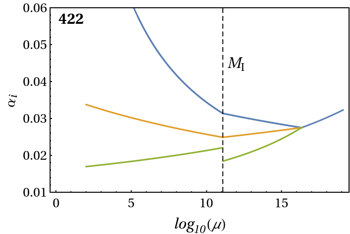
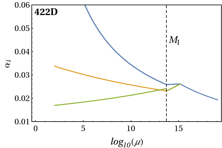
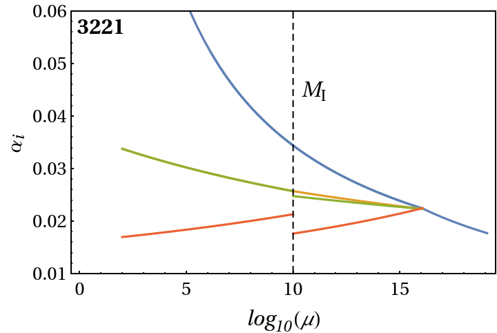
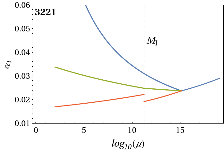
Figure 1: The RG evolution of gauge couplings from the Electroweak scale to the limit close to the Planck scale is shown for the four cases. Top left: 422. Top right: 422D. Bottom left: 3221. Bottom right: 3221D.

At this point we should note that the breaking of the CG to EG given in eq. (23) gives a negative contribution to the cosmological constant and, if this was the only contribution, the space would be AdS. However, we have contributions to the cosmological constant from the other spontaneous breakings of the theory, i.e. the those of $SO(18)$ and $SO(12)$, which are positive. By choosing either of these breakings to be at the same scale with the breaking of the conformal gravity, the various contributions can be fine tuned to give a value for the cosmological constant of either zero or slightly positive, in agreement with the experimental observation.

We will examine three different scenaria regarding the breakings above the GUT scale. In the first, named scenario A, the $SO(18)$ gauge group breaks into $SO(6)\times SO(12)$ and they consequently break into EG and $SO(10)$ (and the global $U(1)$), all at the same scale, $M_{X}$. This way, it is the contribution from the $SO(18)$ breaking to the cosmological constant that cancels the negative one that comes from the CG breaking. In contrast, in the scenaria B and C, the $SO(18)$ gauge group breaks into $SO(6)\times SO(12)$ at a scale $M_{B}$, while both $SO(6)$ and $SO(12)$ will break at a different scale, $M_{X}$, which will be of course between $M_{GUT}$ and $M_{B}$. The hierarchy among the scales is shown in Fig. 2.

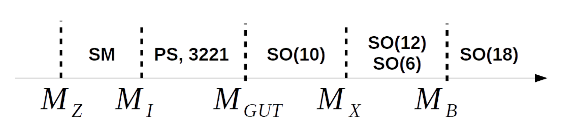
Figure 2: The hierarchy among the various symmetry breaking scales of the models and the respective gauge groups that act on each energy regime.

It is important to note that, while for the evolution of the couplings after the breaking of $SO(10)$ the calculation is clear and we can determine the renormalization group equations (RGEs) in a straightforward way, when we turn to the running of gauge theories based on non-compact groups, the situation certainly is not clear. There exist serious calculations of the $\beta$-functions of the various terms of Stelle’s $R^{2}$ gravity, which was proven to be renormalizable [69, 70], but all calculations are done in Euclidean space [71, 72, 73, 74, 75, 76]. Therefore, strictly speaking the calculation of the $\beta$-function of a gauge theory based on a non-compact group has not been done. We speculate though that at least at one-loop level, the $\beta$-functions of gauge theories of non-compact groups could be well approximated by the corresponding ones of the compact ones. This speculation finds support from the suggestions of Donoghue in a number of papers [77, 78, 79], which we adapt in the corresponding calculations of the $\beta$-functions presented in the Appendix.

Starting from scenario A, if we run the $SO(10)$ gauge coupling until the $M_{X}$ scale, there it will match the value of the $SO(6)$ and $SO(12)$ gauge couplings, so

$$\alpha_{10}^{(1)}(M_{X})=\alpha_{CG}^{(1)}(M_{X})~.$$ (38)

Considering the last term of Eq. (16) and substituting the above relation, we can compare this term with the $SO(18)$ contributions to the cosmological constant. This way we can have an estimate of the breaking scale:

$$M_{X}\sim 10^{18}~\text{GeV}~.$$ (39)

The precise value depends on various parameters, but the order of magnitude should remain as above. However, trying to run the $SO(18)$ coupling up to the Planck scale, we see that its steep RGE moves it almost immediately in the non-perturbative regime and it has a Landau pole lower than the Planck scale. As a consequence, for this scenario to work one would need to either drastically change the field content, or include additional new physics phenomena below the Planck scale.

Turning our attention to scenaria B and C, the difference between them is that for scenario B we choose to break $SO(18)$ at a scale lower than the Planck scale, so $M_{B}<M_{Pl}$, while in scenario C $SO(18)$ breaks exactly at the Planck scale, $M_{B}=M_{Pl}$. Then, in both scenaria, the $SO(6)\times SO(12)$ gauge group will run until the breaking scale $M_{X}$, under which we are left with the $SO(10)$ gauge group and EG. Note that $SO(6)$ and $SO(12)$ have to break at the same scale, if we want to keep the cosmological constant fine tuning.

Here we do not have the matching condition of Eq. (38), as we now have $\alpha_{10}^{(1)}(M_{X})=\alpha_{12}^{(1)}(M_{X})$. Thus, using the $\beta$-function of $SO(10)$ and $SO(12)$ and the approximative $\beta$-functions of $SO(6)$, we make a rough estimate of the scale in question, which again is $M_{X}\sim 10^{18}$GeV. For both scenaria, above $M_{X}$ the $SO(12)$ gauge coupling runs smoothly up to $M_{B}$, well within the perturbative regime. This is due to our choice of representations for some of the scalars of the theory (as explained above), since the fact that they are singlets under the CG gauge group avoids unwanted multiplicities during the calculation of the $SO(12)$ gauge $\beta$-function. For scenario B, $M_{B}$ is slightly below the Planck scale, and the $SO(18)$ gauge coupling runs up to $M_{Pl}$ without entering the non-perturbative regime, although its RG evolution is very steep. The runnings for scenaria B and C are can be found in Fig. 3 and Fig. 4, respectively. Once more, all the $\beta$-functions can be found in the Appendix.

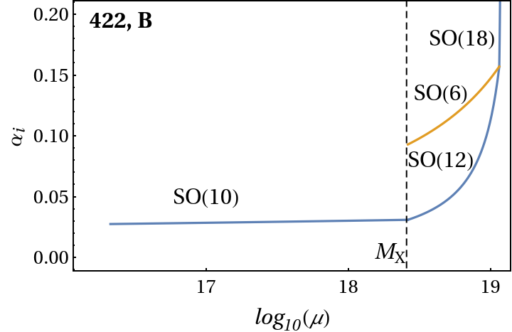
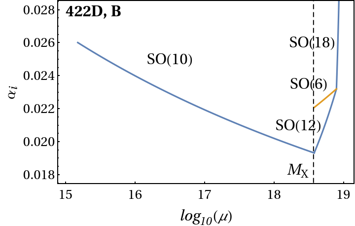
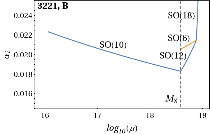
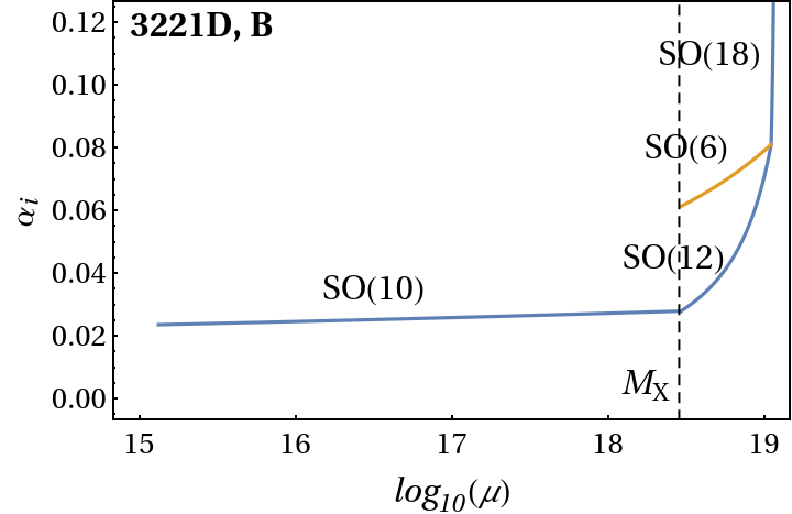
Figure 3: The RG evolution of gauge couplings from the GUT scale up to the Planck scale is shown for the four cases for scenario B. Top left: 422. Top right: 422D. Bottom left: 3221. Bottom right: 3221D.

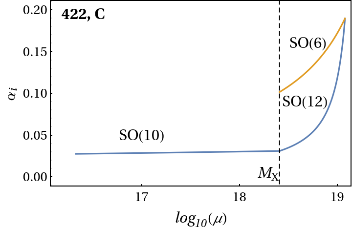
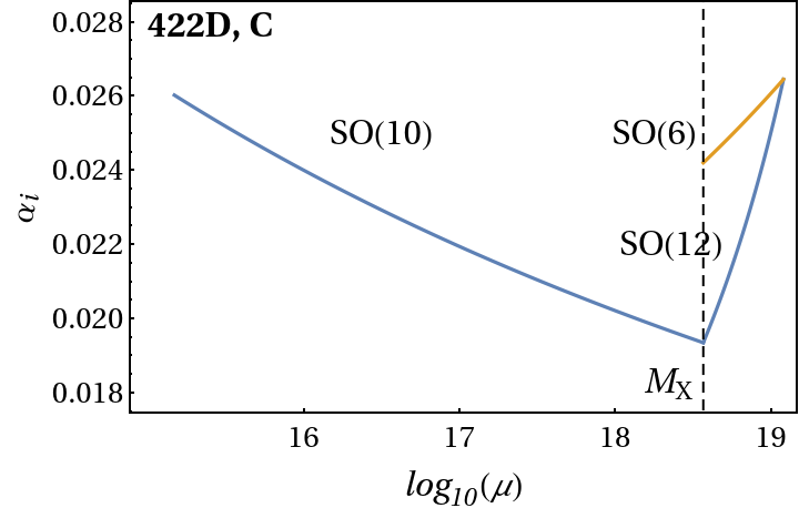
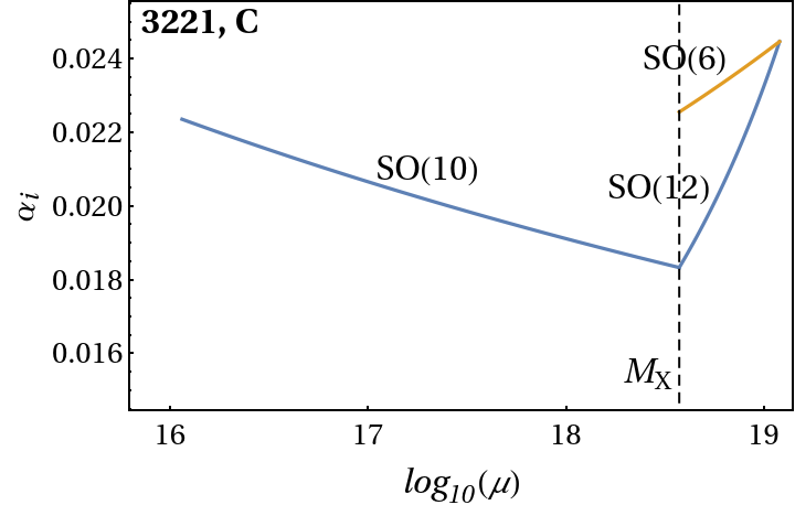
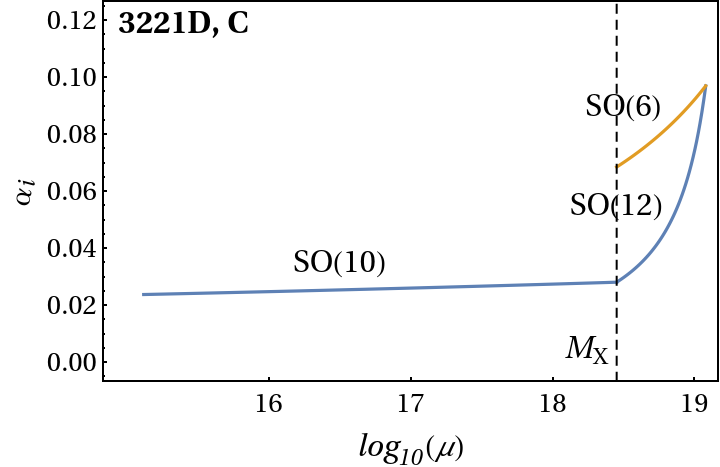
Figure 4: The RG evolution of gauge couplings from the GUT scale up to the Planck scale is shown for the four cases for scenario C. Top left: 422. Top right: 422D. Bottom left: 3221. Bottom right: 3221D.

We would like to add a comment about the case of FG. As it was explained in [49], when attempting to unify FG with internal interactions, along the lines of Unification of Conformal Gravity with $SO(10)$ [33], the difficulties that in principle one is facing are that fermions should (a) be chiral in order to have a chance to survive in low energies and not receive masses as the Planck scale, (b) appear in a matrix representation, since the constructed FG is a matrix model. Then it was suggested [49] and given that the Majorana condition can be imposed, a solution satisfying the conditions (a) and (b) above is the following. We choose to start with the $SO(6)\times SO(12)$ as the initial gauge theory with fermions in the $(\overline{\textbf{4}},\textbf{32})$ representation satisfying in this way the criteria to obtain chiral fermions in tensorial representation of a fuzzy space. Another important point is that using the gauge-theoretic formulation of gravity to construct the FG one is led to in gauging the $SO(6)\times U(1)\sim SO(2,4)\times U(1)$. Therefore from this point of view there exist only a small difference as compared to the CG. Since the extra $U(1)$ symmetry of the gravity part is irrelevant to the above calculations, one could identify scenario C to the FG model. Obviously, the notable difference will be that there is no ($SO(18)$) group above the Planck scale, but this does not affect the calculation above.

4 Conclusions and Discussion

In a previous paper [33], a potentially realistic model was constructed based on the idea that unification of gravity and internal interactions in four dimensions can be achieved by gauging an enlarged tangent Lorentz group. This possibility was based on the observation that the dimension of the tangent space is not necessarily equal to the dimension of the corresponding curved manifold. In [33], due to the very interesting fact that gravitational theories can be described by gauge theories, first was constructed the CG in a gauge theoretic manner by gauging the $SO(2,4)$ group. Of particular interest was the fact that the spontaneous symmetry breaking of the constructed CG could lead, among others, to the EG and the WG. Then it is was possible to unify the CG with internal interactions based on the $SO(10)$ GUT (after breaking of $SO(12)$), using the higher-dimensional tangent group $SO(2,16)$. Inclusion of fermions and application suitably the Weyl and Majorana conditions led to a fully unified scheme, which was promised to be examined further concerning its low scale behaviour as well as its cosmological predictions.

In the present work the behaviour of the fully unified theory has been examined in some detail by examining its breakings at three scales, namely (i) the scale that the $SO(18)$ gauge group breaks, $M_{B}$, (ii) the scale where $SO(6)\times SO(12)$ breaks, $M_{X}$, and (iii) the $SO(10)$ unification scale of internal interactions, $M_{GUT}$ (the examination of the model includes the scale that the intermediate gauge groups below the GUT scale break into the SM gauge group, $M_{I}$, and it runs all the way down to the electroweak scale).

This leads to three distinct scenaria. In scenario A we assume $M_{B}=M_{X}$, so $SO(18)$ breaks immediately to $SO(10)$ and EG, and CG and $SO(12)$ do not run. In scenario B none of the above-mentioned scales coincide, so all different gauge structures run in their respective energy regimes. In scenario C, we identify $M_{B}=M_{Pl}$, so there is no $SO(18)$ running below the Panck scale. The running of the usual internal, i.e. non-gravitational interactions, has been also examined below the $SO(10)$ breaking scale. In particular, gauge couplings run down to the scale that the intermediate gauge groups break, $M_{I}$, and in turn the SM gauge couplings are run all the way down to the electroweak scale. The result is that the proposed in [33] unification scheme of all interactions, including gravity in the form of CG, which subsequently was broken to EG is a realistic one and can be examined perturbatively for scenaria B and C, while we provide an estimate of all the symmetry breaking scales for each case. The FG case exhibits the same behaviour as scenario C.

In the future we plan to study the cosmological implications of the constructed Unified scheme. In particular we plan to do studies along those done in the ghost-free bigravity [80] and of E. Kolb and collaborators [81]. A more immediate examination concerns the implications of the various spontaneous symmetry breakings discussed in the present paper in the formation of cosmic strings and their possible gravitational wave signal along the study of [82].

It is always useful to repeat the reason that the present unified scheme overcomes the Coleman–Mandula (CM) theorem [83]. The point being that the CM theorem has several hypotheses and the most relevant is that the theory is Poincaré invariant. In [33], given that the final aim was to obtain the Einstein gravitational theory coupled to the GUTs, obviously the original conformal group, which is an extension of the Poincaré group was spontaneously broken to the Lorentz group.

Appendix: $\beta$-Functions of the Gauge Couplings at each Energy Sale

In this section we give all the one-loop $\beta$-functions of the gauge couplings of all gauge groups -with the appropriate field content each time- that we encounter after the various spontaneous symmetry breakings mentioned above. They are given by:

$$\beta_{g_{i}}=16\pi^{2}\mu\frac{d}{d\mu}g_{i}=b_{i}g_{i}^{3}\quad\quad\text{or}\quad\quad\beta_{\alpha_{i}}=2\pi\mu\frac{d}{d\mu}\alpha_{i}=b_{i}\alpha_{i}^{2}~,$$ (40)

where $\alpha_{i}=g_{i}^{2}/4\pi$ and $b_{i}$ is the respective $\beta$-function coefficient, which is the quantity we need to calculate in each case.

Considering the group-theoretical details of all three SM gauge groups well-known, we can give their respective $\beta$-function coefficients:

$$b_{3}= -7$$ (41)

$$b_{2}= -\frac{19}{6}$$ (42)

$$b_{1}= \frac{41}{10}~,$$ (43)

where the $b_{1}$ ocoefficient is given in the usual $SU(5)$ normalization.

For the four intermediate gauge groups using the usual way of [84], the $b_{i}$ coefficients can be easily found to be:

442:

• $b_{4}=-\frac{7}{3}$

• $b_{2L}=2$

• $b_{2R}=\frac{28}{3}$

a

442D:

• $b_{4}=\frac{2}{3}$

• $b_{2L}=\frac{28}{3}$

• $b_{2R}=\frac{28}{3}$

a

3221:

• $b_{3}=-7$

• $b_{2L}=-\frac{8}{3}$

• $b_{2R}=-2$

• $b_{1}=\frac{11}{2}$

3221D:

• $b_{3}=-7$

• $b_{2L}=-\frac{4}{3}$

• $b_{2R}=-\frac{4}{3}$

• $b_{1}=7$

For the bigger groups that feature in the above theory, we give a list of a few details that are necessary for the calculation of their $b_{i}$’s:

$SO(6)$:

• Generators:
  $N^{2}-1=15$

• $C_{2}(\textbf{15})=4$

• $T(\textbf{15})=4$

• $T(\textbf{4})=1/2$

a
a
a
a
a
a

$SO(10)$:

• Generators:
  $N(N-1)/2=45$

• $C_{2}(\textbf{45})=$
  $T(\textbf{45})=8$

• $T(\textbf{16})=2$

• $T(\textbf{10})=1$

• $T(\textbf{54})=12$

• $T(\textbf{126})=35$

• $T(\textbf{210})=56$

a

$SO(12)$:

• Generators:
  $N(N-1)/2=66$

• $C_{2}(\textbf{66})=$
  $T(\textbf{66})=10$

• $T(\textbf{12})=1$

• $T(\textbf{32})=4$

• $T(\textbf{77})=14$

• $T(\textbf{495})=120$

• $T(\textbf{792})=210$

a

$SO(18)$:

• Generators:
  $N(N-1)/2=153$

• $C_{2}(\textbf{153})=$
  $T(\textbf{153})=16$

• $T(\textbf{18})=1$

• $T(\textbf{170})=20$

• $T(\textbf{256})=32$

• $T(\textbf{3060})=$
  $560$

• $T(\textbf{8568})=$
  $1820$

With this information at hand, we can now calculate their respective $b_{i}$ coefficients for each intermediate breaking scenario:

$SO(10)$:

• $b_{10}^{422}=\frac{16}{3}$

• $b_{10}^{422D}=-\frac{28}{3}$

• $b_{10}^{3221}=-\frac{32}{3}$

• $b_{10}^{3221D}=\frac{16}{3}$

$SO(12)$:

• $b_{12}^{422}=\frac{331}{3}$

• $b_{12}^{422D}=75$

• $b_{12}^{3221}=\frac{221}{3}$

• $b_{12}^{3221D}=\frac{331}{3}$

$SO(6)$:

• $b_{6}^{422}=4$

• $b_{6}^{422D}=4$

• $b_{6}^{3221}=4$

• $b_{6}^{3221D}=4$

$SO(18)$:

• $b_{18}^{422}=-$

• $b_{18}^{422D}=-$

• $b_{18}^{3221}=-$

• $b_{18}^{3221D}=-$

One can see that, since all the scalars that break the intermediate symmetries at $M_{I}$ are singlets under the CG group, its $b_{i}$’s will be the same for each case.

References

- [1] T. Kaluza, Sitzungsber. Preuss. Akad. Wiss. Berlin (Math. Phys.) , 966 (1921).
- [2] O. Klein, Z. Phys. 37, 895 (1926).
- [3] R. Kerner, Ann. Inst. H. Poincare Phys. Theor. 9, 143 (1968).
- [4] Y. Cho, J. Math. Phys. 16, 2029 (1975).
- [5] Y. Cho and P. Freund, Phys. Rev. D 12, 1711 (1975).
- [6] E. Witten, Conf. Proc. C 8306011, 227 (1983).
- [7] H. Georgi, Lie Algebras In Particle Physics: from Isospin To Unified Theories (1999).
- [8] H. Fritzsch and P. Minkowski, Ann. Phys. 93, 193 (1975).
- [9] G. Chapline and R. Slansky, Nucl. Phys. B 209, 461 (1982).
- [10] M. Green, J. Schwarz, and E. Witten, Superstring Theory, Vol 1 & 2 (1988).
- [11] J. Polchinski, String theory, Vol 1 & 2 (1998).
- [12] D. Lust and S. Theisen, Lectures on String Theory, Vol 346 (1989).
- [13] D. Gross, J. Harvey, E. Martinec, and R. Rohm, Nucl. Phys. B 256, 253 (1985).
- [14] P. Forgåcs and N. Manton, Commun. Math. Phys. 72, 15 (1980).
- [15] N. Manton, Nucl. Phys. B 193, 502 (1981).
- [16] Y. Kubyshin, I. Volobuev, J. Mourao, and G. Rudolph, Dimensional Reduction of Gauge Theories, Spontaneous Compactification and Model Building, Vol 349 (1989).
- [17] D. Kapetanakis and G. Zoupanos, Phys. Rept. 219, 4 (1992).
- [18] D. Lust and G. Zoupanos, Phys. Lett. B 165, 309 (1985).
- [19] J. Scherk and J. Schwarz, Nucl. Phys. B 153, 61 (1979).
- [20] P. Manousselis and G. Zoupanos, JHEP 2004, 025 (2004).
- [21] A. Chatzistavrakidis and G. Zoupanos, JHEP 09, 077 (2009).
- [22] N. Irges and G. Zoupanos, Phys. Lett. B 698, 146 (2011).
- [23] G. Manolakos, G. Patellis, and G. Zoupanos, Phys. Lett. B 813, 136031 (2021), arXiv:2009.07059.
- [24] G. Patellis, W. Porod, and G. Zoupanos, JHEP 01, 021 (2024), arXiv:2307.10014.
- [25] R. Utiyama, Phys. Rev. 101, 1597 (1956).
- [26] T. Kibble, J. Math. Phys. 2, 212 (1961).
- [27] S. MacDowell and F. Mansouri, Phys. Rev. Lett. 38, 739 (1977).
- [28] E. A. Ivanov and J. Niederle, On Gauge Formulations Of Gravitation Theories., in 9th International Colloquium on Group Theoretical Methods in Physics, pp. 545–551, 1980.
- [29] E. Ivanov and J. Niederle, Phys. Rev. D 25, 976 (1982).
- [30] K. Stelle and P. West, Phys. Rev. D 21, 1466 (1980).
- [31] T. Kibble and K. Stelle, Progress In Quantum Field Theory (1985), Report number: Imperial-TP-84-85-13.
- [32] M. Kaku, P. Townsend, and P. van Nieuwenhuizen, Phys. Rev. D 17, 3179 (1978).
- [33] D. Roumelioti, S. Stefas, and G. Zoupanos, Eur. Phys. J. C 84, 577 (2024), arXiv:2403.17511.
- [34] E. Fradkin and A. Tseytlin, Phys. Rept. 119, 233 (1985).
- [35] J. Maldacena, (2011), arXiv:1105.5632, e-Print: 1105.5632 [hep-th].
- [36] P. D. Mannheim, Found. Phys. 42, 388 (2012), arXiv:1101.2186.
- [37] G. Anastasiou and R. Olea, Phys. Rev. D 94, 086008 (2016), arXiv:1608.07826.
- [38] D. M. Ghilencea, JHEP 03, 049 (2019), arXiv:1812.08613.
- [39] A. Hell, D. Lust, and G. Zoupanos, JHEP 08, 168 (2023), arXiv:2306.13714.
- [40] D. M. Ghilencea, JHEP 10, 113 (2023), arXiv:2309.11372.
- [41] D. Freedman and A. Van Proeyen, Supergravity (Cambridge University Press, 2012).
- [42] T. Ortin, Gravity and Strings, Cambridge Monographs on Mathematical Physics, 2nd ed. ed. (Cambridge University Press, 2015).
- [43] L. Castellani, Phys. Rev. D 88, 025022 (2013), arXiv:1301.1642.
- [44] A. Chatzistavrakidis et al., Fortsch. Phys. 66, 1800047 (2018).
- [45] G. Manolakos, P. Manousselis, and G. Zoupanos, JHEP 08, 001 (2020), arXiv:1902.10922.
- [46] G. Manolakos, P. Manousselis, and G. Zoupanos, Fortsch. Phys. 69, 2100085 (2021).
- [47] G. Manolakos, P. Manousselis, D. Roumelioti, S. Stefas, and G. Zoupanos, Universe 8, 215 (2022).
- [48] G. Manolakos, P. Manousselis, D. Roumelioti, S. Stefas, and G. Zoupanos, Eur.Phys.J.ST 232, 3607 (2023), arXiv:2305.11785.
- [49] D. Roumelioti, S. Stefas, and G. Zoupanos, Fortsch. Phys. 72, 2400126 (2024), arXiv:2407.07044.
- [50] R. Percacci, Phys. Lett. B 144, 37 (1984).
- [51] R. Percacci, Nucl. Phys. B 353, 271 (1991).
- [52] F. Nesti and R. Percacci, J.Phys.A 41, 075405 (2008).
- [53] F. Nesti and R. Percacci, Phys. Rev. D 81, 025010 (2010).
- [54] K. Krasnov and R. Percacci, Class. Quant. Grav. 35, 143001 (2018).
- [55] A. Chamseddine and V. Mukhanov, JHEP 03, 033 (2010).
- [56] A. Chamseddine and V. Mukhanov, JHEP 03, 020 (2016).
- [57] P. Schupp, K. Anagnostopoulos, and G. Zoupanos, Eur.Phys.J.ST 232, 1 (2024).
- [58] S. Konitopoulos, D. Roumelioti, and G. Zoupanos, Fortsch. Phys. 2023, 2300226 (2023), arXiv:2309.15892.
- [59] S. Weinberg, Generalized Theories Of Gravity And Supergravity In Higher Dimensions, in Fifth Workshop on Grand Unification, 1984.
- [60] G. Manolakos, Construction of gravitational models as noncommutative gauge theories, PhD thesis, Natl. Tech. U., Athens, 2019.
- [61] R. Slansky, Phys. Rept. 79, 1 (1981).
- [62] R. Feger, T. W. Kephart, and R. J. Saskowski, Comput. Phys. Commun. 257, 107490 (2020), arXiv:1912.10969.
- [63] L.-F. Li, Phys. Rev. D 9, 1723 (1974).
- [64] A. Chamseddine, J. Math. Phys. 44, 2534 (2003), arXiv:hep-th/0202137.
- [65] R. D’Auria, S. Ferrara, M. Lledó, and V. Varadarajan, J. Geom. Phys. 40, 101 (2001).
- [66] J. Figueroa-O’Farrill, Majorana spinors, https://www.maths.ed.ac.uk/ jmf/Teaching/ Lectures/Majorana.pdf.
- [67] A. Djouadi, R. Fonseca, R. Ouyang, and M. Raidal, Eur. Phys. J. C 83, 529 (2023).
- [68] Particle Data Group, R. L. Workman et al., PTEP 2022, 083C01 (2022).
- [69] K. S. Stelle, Phys. Rev. D 16, 953 (1977).
- [70] K. S. Stelle, Gen. Rel. Grav. 9, 353 (1978).
- [71] E. S. Fradkin and A. A. Tseytlin, Nucl. Phys. B 201, 469 (1982).
- [72] I. G. Avramidi and A. O. Barvinsky, Phys. Lett. B 159, 269 (1985).
- [73] A. Codello and R. Percacci, Phys. Rev. Lett. 97, 221301 (2006), arXiv:hep-th/0607128.
- [74] M. R. Niedermaier, Phys. Rev. Lett. 103, 101303 (2009).
- [75] M. Niedermaier, Nucl. Phys. B 833, 226 (2010).
- [76] N. Ohta and R. Percacci, Class. Quant. Grav. 31, 015024 (2014), arXiv:1308.3398.
- [77] J. F. Donoghue, Phys. Rev. D 96, 044006 (2017), arXiv:1609.03524.
- [78] J. F. Donoghue, Phys. Rev. D 96, 044003 (2017), arXiv:1609.03523.
- [79] J. F. Donoghue, Phys. Rev. D 96, 044007 (2017), arXiv:1704.01533.
- [80] S. Hassan, A. Schmidt-May, and M. von Strauss, Universe 1, 92 (2015).
- [81] E. Kolb, S. Ling, A. Long, and R. Rosen, JHEP 05, 181 (2023).
- [82] S. F. King, S. Pascoli, J. Turner, and Y.-L. Zhou, JHEP 10, 225 (2021), arXiv:2106.15634.
- [83] S. Coleman and J. Mandula, Phys. Rev. 159, 1251 (1967).
- [84] D. R. T. Jones, Phys. Rev. D 25, 581 (1982).