Methods with Local Steps and Random Reshuffling for Generally Smooth Non-Convex Federated Optimization

Abstract

Non-convex Machine Learning problems typically do not adhere to the standard smoothness assumption. Based on empirical findings, Zhang et al. (2020b) proposed a more realistic generalized $(L_{0},L_{1})$-smoothness assumption, though it remains largely unexplored. Many existing algorithms designed for standard smooth problems need to be revised. However, in the context of Federated Learning, only a few works address this problem but rely on additional limiting assumptions. In this paper, we address this gap in the literature: we propose and analyze new methods with local steps, partial participation of clients, and Random Reshuffling without extra restrictive assumptions beyond generalized smoothness. The proposed methods are based on the proper interplay between clients’ and server’s stepsizes and gradient clipping. Furthermore, we perform the first analysis of these methods under the Polyak-Łojasiewicz condition. Our theory is consistent with the known results for standard smooth problems, and our experimental results support the theoretical insights.

1 Introduction

Distributed optimization problems and distributed algorithms have gained a lot of attention in recent years in the Machine Learning (ML) community. In particular, modern problems often lead to the training of deep neural networks with billions of parameters on large datasets (Brown et al., 2020; Kolesnikov et al., 2019). To make the training time feasible (Li, 2020), it is natural to parallelize computations (e.g., stochastic gradients computations), i.e., apply distributed training algorithms (Goyal et al., 2017; You et al., 2019; Le Scao et al., 2023). Another motivation for the usage of distributed methods is dictated by the fact that data can be naturally distributed across multiple devices/clients and be private, which is a typical scenario in Federated Learning (FL) (Konecný et al., 2016; McMahan et al., 2016; Kairouz et al., 2019).

Typically, such problems are not $L$-smooth as indicated by Defazio & Bottou (2019) that motivated the optimization researchers to study so-called generalized smoothness assumptions. In particular, Zhang et al. (2020b) propose $(L_{0},L_{1})$-smoothness assumption, which allows the norm of the Hessian to grow linearly with the norm of the gradient, and empirically validate it for several problems involving the training of neural networks. In addition, Ahn et al. (2023); Crawshaw et al. (2024); Wang et al. (2024) demonstrate that linear transformers with few layers satisfy this assumption, highlighting the practical importance of $(L_{0},L_{1})$-smoothness. Moreover, the theoretical convergence of different methods is studied under $(L_{0},L_{1})$-smoothness in the literature (Zhang et al., 2020b, a; Koloskova et al., 2023a; Chen et al., 2023; Li et al., 2024a, b; Crawshaw et al., 2024). Noticeably, most of these methods utilize gradient clipping (Pascanu et al., 2013).

However, in the context of Distributed/Federated Learning, the theoretical convergence of methods is weakly explored under $(L_{0},L_{1})$-smoothness. In particular, only a couple of papers analyze methods with local steps and Random Reshuffling – two highly important techniques in FL – under $(L_{0},L_{1})$-smoothness but only with additional restrictive assumptions such as data homogeneity (Liu et al., 2022), bounded variance (Wang et al., 2024) or cosine relatedness (Qian et al., 2021). Moreover, to the best of our knowledge, there are no results for the methods with partial participation of clients under $(L_{0},L_{1})$-smoothness. Such a noticeable gap in the literature leads us to the question: is it possible to design methods with local steps, Random Reshuffling, and partial participation of clients with provable convergence guarantees under $(L_{0},L_{1})$-smoothness without additional restrictive assumptions? In this paper, we give a positive answer to this question.

1.1 Our contributions

• New method with local steps. We propose a new method with local steps called Clip-LocalGDJ (Algorithm 1). This method can be seen as a version of LocalGD (Mangasarian, 1995; McMahan et al., 2016) with different clients and server stepsizes and (smoothed) gradient clipping (Pascanu et al., 2013) on a server side. We also prove the convergence of Clip-LocalGDJ for distributed non-convex $(L_{0},L_{1})$-smooth problems without additional assumptions such as data homogeneity used in the previous works (Liu et al., 2022).

• New method with local steps and Random Reshuffling. The second method we propose – CLERR (Algorithm 2) – utilizes local steps and Random Reshuffling and clipping once-in-a-epoch. For the new method, we derive rigorous convergence bounds for distributed non-convex $(L_{0},L_{1})$-smooth problems without additional assumptions such as bounded variance (Wang et al., 2024) or cosine relatedness (Qian et al., 2021).

• New method with local steps, Random Reshuffling, and partial participation. We extend RR-CLI (Malinovsky et al., 2023a), utilizing Random Reshuffling of clients (as an alternative to clients’ sampling) and clients’ data at each meta-epoch, and adjust it to the case of $(L_{0},L_{1})$-smooth objectives through the usage of (smoothed) gradient clipping at the end of each meta-epoch. For the resulting method called Clipped RR-CLI (Algorithm 3), we derive a convergence rate for distributed non-convex $(L_{0},L_{1})$-smooth problems without additional restrictive assumptions. To the best of our knowledge, this is the first result for an FL method with partial participation of clients under $(L_{0},L_{1})$-smoothness assumption.

• Results for the PŁ-functions. For all three new methods, we derive new results under Polyak-Łojasiewicz condition (Polyak, 1963; Lojasiewicz, 1963) that, to the best of our knowledge, are the first results for FL methods under $(L_{0},L_{1})$-smoothness and Polyak-Łojasiewicz condition. The analysis is based on the careful consideration of two possible cases (the gradient is either “small” or “big”) and induction proof of the boundedness of certain metrics.

• Tightness of the results. The derived results are tight: in the special case of $L$-smooth functions, our results recover the known ones for the non-clipped version of the algorithms.

• Numerical experiments. Our numerical experiments illustrate the superiority of the proposed methods over the existing baselines.

1.2 Preliminaries

In this paper, we consider a standard distributed optimization problem

$$\min_{x\in\mathbb{R}^{d}}\left\{f(x)\overset{\text{def}}{=}\frac{1}{M}\sum_{m=1}^{M}f_{m}(x)\right\},$$ (1)

where $[M]\overset{\text{def}}{=}\{1,2,\ldots,M\}$ represents the set of all workers participating in the training, and each $f_{m}:\mathbb{R}^{d}\to\mathbb{R}$ is a non-convex function corresponding to the loss computed on the data available on client $m$ for the current model parameterized by $x\in\mathbb{R}^{d}$. Throughout the paper, we consider two setups: either workers can compute the full gradient $\nabla f_{m}(x)$ of their loss functions or they can compute only a stochastic gradient at each step. In the latter case, we will assume that functions $\{f_{m}\}_{m=1}^{M}$ have the finite-sum form

$$f_{m}(x)=\frac{1}{N}\sum_{j=1}^{N}f_{mj}(x),\quad\forall m\in[M],$$

where $f_{mj}(x)$ corresponds to the local loss of the current model parameterized by $x\in\mathbb{R}^{d},$ evaluated for the $j$-th data point on the dataset belonging to the $m$-th client.

1.3 Related Work

Local training.

Local Training (LT), where clients perform multiple optimization steps on their local data before engaging in the resource-intensive process of parameter synchronization, stands out as one of the most effective and practical techniques for training FL models. LT was proposed by Mangasarian (1995); Povey et al. (2014); Moritz et al. (2015) and later promoted by McMahan et al. (2016). Early theoretical analyses of LT methods relied on restrictive data homogeneity assumptions, which are often unrealistic in real-world federated learning (FL) settings (Stich, 2018; Li et al., 2019; Haddadpour & Mahdavi, 2019). Later, Khaled et al. (2019a, b) removed limiting data homogeneity assumptions for LocalGD (Gradient Descent (GD) with LT). Then, Woodworth et al. (2020); Glasgow et al. (2022) derived lower bounds for GD with LT and data sampling, showing that its communication complexity is no better than minibatch Stochastic Gradient Descent (SGD) in settings with heterogeneous data. Another line of works focused on the mitigating so-called client drift phenomenon, which naturally occurs in LocalGD applied to distributed problems with heterogeneous local functions (Karimireddy et al., 2020; Gorbunov et al., 2021b; Mishchenko et al., 2022; Malinovsky et al., 2023b).

Random reshuffling.

Although standard Stochastic Gradient Descent (SGD) (Robbins & Monro, 1951) is well-understood from a theoretical perspective (Rakhlin et al., 2012; Bottou et al., 2018; Nguyen et al., 2018; Gower et al., 2019; Drori & Shamir, 2020; Khaled & Richtárik, 2020; Demidovich et al., 2024), most widely-used ML frameworks rely on sampling without replacement, as it works better in the training neural networks (Bottou, 2009; Recht & Ré, 2013; Bengio, 2012; Sun, 2020). It leverages the finite-sum structure by ensuring each function is used once per epoch. However, this introduces bias: individual steps may not reflect full gradient descent steps on average. Thus, proving convergence requires more advanced techniques. Three popular variants of sampling without replacement are commonly used. Random Reshuffling (RR), where the training data is randomly reshuffled before the start of every epoch, is an extremely popular and well-studied approach. The aim of RR is to disrupt any potentially untoward default data sequencing that could hinder training efficiency. RR works very well in practice. Shuffle Once (SO) is analogous to RR, however, the training data is permuted randomly only once prior to the training process. The empirical performance is similar to RR. Incremental Gradient (IG) is identical to SO with the difference that the initial permutation is deterministic. This approach is the simplest, however, ineffective. IG has been extensively studied over a long period (Luo, 1991; Grippo, 1994; Li et al., 2022; Ying et al., 2019; Gürbüzbalaban et al., 2019; Nguyen et al., 2021). A major challenge with IG lies in selecting a particular permutation for cycling through the iterations, a task that Nedic & Bertsekas (2001) highlight as being quite difficult. (Bertsekas, 2015) provides an example that underscores the vulnerability of IG to poor orderings, especially when contrasted with RR. Meaningful theoretical analyses of the SO method have only emerged recently (Safran & Shamir, 2020; Rajput et al., 2020). RR has been shown to outperform both SGD and IG for objectives that are twice-smooth (Gürbüzbalaban et al., 2015; Haochen & Sra, 2019). Jain et al. (2019) examine the convergence of RR for smooth objectives. Safran & Shamir (2020); Rajput et al. (2020) provide lower bounds for RR. Mishchenko et al. (2020) recently conducted a thorough analysis of IG, SO and RR using innovative and simplified proof techniques, resulting in better convergence rates.

Generalized smoothness.

Let us remind that the function $f$ is said to be $L$-smooth if there exist $L\geq 0$ such that $\left\lVert\nabla f(x)-\nabla f(y)\right\rVert\leq L\left\lVert x-y\right\rVert$ for all $x,y\in\mathbb{R}^{d}.$ For twice-differentiable functions, it is equivalent to $\left\lVert\nabla^{2}f(x)\right\rVert\leq L,$ for all $x\in\mathbb{R}^{d}.$ This assumption is very standard in the optimization field. Recently, based on extensive experiments, Zhang et al. (2020b) introduced a generalization of this condition called $(L_{0},L_{1})$-smoothness. Namely, twice-differentiable function $f$ is said to be $(L_{0},L_{1})$-smooth if $\left\lVert\nabla^{2}f(x)\right\rVert\leq L_{0}+L_{1}\left\lVert\nabla f(x)\right\rVert,$ for all $x\in\mathbb{R}^{d}.$ Compared to the standard smoothness, this condition is its strict relaxation, and it is applied to a broader range of functions. Zhang et al. (2020b) demonstrated empirically that generalized smoothness provides a more accurate representation of real-world task objectives, especially in the context of training deep neural networks. During LSTM training, it was noted that the local Lipschitz constant $L_{0}$ near the stationary point is thousands of times smaller than the global Lipschitz constant $L$. Under this condition, Zhang et al. (2020b) provided a theoretical justification for the gradient clipping technique (Pascanu et al., 2013), which is considered effective in mitigating the issue of exploding gradients. Their results were improved by (Zhang et al., 2020a; Koloskova et al., 2023a). (Chen et al., 2023) establish various useful properties of generalized-smooth functions, propose generalizations of $(L_{0},L_{1})$-smoothness and optimal first-order algorithms for solving generalized-smooth non-convex problems. Li et al. (2024a, b) extend the $(L_{0},L_{1})$-smoothness condition, introduce a novel analysis technique that bounds gradients along the trajectory, analyze GD, SGD, Nesterov’s accelerated gradient method and Adam. (Crawshaw et al., 2024) consider a coordinate-wise version of generalized smoothness. (Gorbunov et al., 2024) consider (strongly) convex case for Clipped GD and provide tighter rates as well as propose a new accelerated method, derive rates for several adaptive methods. (Ahn et al., 2023; Crawshaw et al., 2024; Wang et al., 2024) demonstrate that linear transformers with few layers satisfy generalized smoothness empirically. There are few papers on distributed algorithms that combine local steps or reshuffling with generalized smoothness. Qian et al. (2021) examined clipped IG; Wang et al. (2024) investigated Adam with RR; (Liu et al., 2022) studied LocalGD, however, all of the papers contain additional restrictive assumptions. This is a significant gap in the literature and we close it in our paper.

Algorithm 1 Clip-LocalGDJ: Clipped Local Gradient Descent with Jumping

1: Input: Synchronization/communication times $0=t_{0}<t_{1}<t_{2}<\ldots<t_{P-1}$, initial vector $x_{0}\in\mathbb{R}^{d},$ number of epochs $P\geq 1,$ constants $c_{0},c_{1}>0.$

2: Initialize $x_{0}^{m}=\hat{x}_{0}=x_{0}$ for all $m\in[M]\overset{\text{def}}{=}\{1,2,\dots,M\}.$

3: for $p=0,1,\ldots,P-1$ do

4:  Choose the server stepsize $\gamma_{p}=\frac{1}{c_{0}+c_{1}\left\lVert\nabla f(\hat{x}_{t_{p}})\right\rVert}.$

5:  Choose small inner stepsize $\alpha_{p}>0.$

6:  for $m=1,\dots,M$ do

7:   $x_{t_{p}}^{m}=\hat{x}_{t_{p}}$

8:   for $t\in\{t_{p},\ldots t_{p+1}-2\}$ do

9:    $x_{t+1}^{m}=x_{t}^{m}-\alpha_{p}\nabla f_{m}(x_{t}^{m})$

10:   end for

11:  end for

12:  $g_{p}=\frac{1}{\alpha_{p}\left(t_{p+1}-1-t_{p}\right)}\left(\hat{x}_{t_{p}}-\frac{1}{M}\sum_{m=1}^{M}x_{t_{p+1}-1}^{m}\right)$

13:  $\hat{x}_{t_{p+1}}=\hat{x}_{t_{p}}-\gamma_{p}g_{p}$

14: end for

2 New methods

In this section, we introduce the new methods – Clip-LocalGDJ (Algorithm 1), CLERR (Algorithm 2), and Clipped RR-CLI (Algorithm 3).

Clip-LocalGDJ.

As standard LocalGD, the first method (Clip-LocalGDJ, Algorithm 1) alternates between local GD steps on each worker and synchronization/averaging steps. However, there are two noticeable differences between Clip-LocalGDJ and LocalGD. The first one is the usage of different clients’ and server’s stepsizes. In our method, clients’ stepsizes are typically smaller than the server’s ones, which allows us to handle the client drift. Then, on the server, the pseudogradient $g_{p}$ is computed, and the server performs a Clip-GD-type step, which is a second important difference compared to LocalGD. Since the server’s stepsize is typically larger than the clients’ stepsizes, the local steps can be seen as steps determining the update direction, and the server step can be seen as a larger “jump” in the averaged update direction.

CLERR.

In CLERR (Algorithm 2), each client does a full epoch of RR before between synchronization steps (similarly to (Malinovsky et al., 2023b)), and similarly to Clip-LocalGDJ, (smoothed) clipping is applied only to the averaged pseudogradient $g_{t}$ once in an epoch. In contrast, a naïve combination of clipping with RR uses clipping at each step, which can amplify the bias of RR and lead to poor performance (as we illustrate in our experiments).

Algorithm 2 CLERR: Clipped once in an Epoch Random Reshuffling

1: Input: Starting point $x_{0}\in\mathbb{R}^{d}$, number of epochs $T,$ constants $c_{0},c_{1}>0.$

2: for $t=0,\dots,T-1$ do

3:  Choose global stepsize $\gamma_{t}=\frac{1}{c_{0}+c_{1}\left\|\nabla f(x_{t})\right\|}.$

4:  Choose small inner stepsize $\alpha_{t}>0.$

5:  Sample a permutation $\pi_{t}=\left\{\pi_{t}(1),\dots,\pi_{t}(N)\right\}$.

6:  for $m=1,\dots,M$ do

7:   $x_{t,0}^{m}=x_{t}$

8:   for $j=0,\dots,N-1$ do

9:    $x_{t,j+1}^{m}=x_{t,j}^{m}-\alpha_{t}\nabla f_{m,\pi_{t}(j)}(x_{t,j}^{m})$.

10:   end for

11:   $g_{t}^{m}=\frac{1}{\alpha_{t}N}(x_{t}-x_{t,N}^{m})$

12:  end for

13:  $g_{t}=\frac{1}{M}\sum_{m=1}^{M}g_{t}^{m}$.

14:  $x_{t+1}=x_{t}-\gamma_{t}g_{t}$.

15: end for

Clipped RR-CLI.

Clipped RR-CLI (Algorithm 3) is the first FL algorithm that combines clipping, local steps, local dataset reshuffling, server and client step sizes and regularized client partial participation (sampling of clients without replacement). It is based on RR-CLI proposed by Malinovsky et al. (2023a) and leverages the core techniques proposed in FedAvg (McMahan et al., 2016). The key idea is similar to CLERR, but in addition to the reshuffling of clients’ data, Clipped RR-CLI performs a reshuffling of the groups of clients as an alternative to the standard i.i.d. sampling of clients at each communication round. At the end of each meta-epoch, the server performs a smoothed Clip-GD-type step similar to the one used in CLERR, which allows the method to make a larger step with an accumulated pseudogradient.

When the number of workers is large, partial participation is preferable. In this case, Clipped RR-CLI (Algorithm 3) is the best option as it utilizes partial participation. Otherwise, if we have access to full gradients on the workers, then Clip-LocalGDJ(Algorithm 1) is preferable. In case when the workers can compute only a stochastic gradient, then CLERR (Algorithm 2) is recommended.

Notice that these methods include the computation of the norm of the full gradient in the global stepsize. More practical versions of our methods use pseudogradients $g_{t}$ instead. We employ the stepsizes with pseudogradients in our experiments (see Section 5). In Appendix E we show that our theory covers practical versions as well.

1: Input: cohort size $C\in\{1,2,\dots,M\}$; number of rounds $R=M/C$; initial iterate/model $x_{0}\in\mathbb{R}^{d}$; number of meta-epochs $T\geq 1,$ constants $c_{0},c_{1}>0.$

2: for meta-epoch $t=0,1,\ldots,T-1$ do

3:  Choose global stepsize $\theta_{t}=\frac{1}{c_{0}+c_{1}\left\lVert\nabla f(x_{t})\right\rVert}.$

4:  Choose small server stepsize $\eta_{t}>0.$

5:  Choose small client stepsize $\gamma_{t}>0.$

6:  $x_{t}^{0}=x_{t}$

7:  Client-Reshuffling: sample a permutation $\lambda=(\lambda_{0},\lambda_{1},\ldots,\lambda_{R-1})$ of $[R]$

8:  for communication rounds $r=0,\ldots,R-1$ do

9:   Send model $x^{r}_{t}$ to participating clients $m\in S^{\lambda_{r}}_{t}$ (server broadcasts $x^{r}_{t}$ to clients $m\in S^{\lambda_{r}}_{t}$)

10:   for all clients $m\in S^{\lambda_{r}}_{t}$, locally in parallel do

11:    $x^{r,0}_{m,t}=x^{r}_{t}$ (client $m$ initializes local training using the latest global model $x^{r}_{t}$)

12:    Data-Random-Reshuffling: sample a permutation $\pi_{m}=(\pi^{0}_{m},\pi^{1}_{m},\ldots,\pi^{N-1}_{m})$ of $[N]$

13:    for all local training data points $j=0,1,\ldots,N-1$ do

14:     $x_{m,t}^{r,j+1}=x_{m,t}^{r,j}-\gamma_{t}\nabla f^{\pi^{j}_{m}}_{m}(x_{m,t}^{r,j})$ (client $m$ passes once its local data in $\pi_{m}$ order)

15:    end for

16:    $g^{r}_{m,t}=\frac{1}{\gamma_{t}N}(x^{r}_{t}-x^{r,N}_{m,t})$ (client $m$ computes local update direction $g_{m,t}$)

17:   end for

18:   $g^{r}_{t}=\frac{1}{C}\sum\limits_{m\in S^{\lambda_{r}}_{t}}g^{r}_{m,t}$ (server aggregates local directions $g_{m,t}$ of the clients cohort $S_{t}$)

19:   $x^{r+1}_{t}=x^{r}_{t}-\eta_{t}g^{r}_{t}$ (server updates the model in aggregated direction $g_{t}$ with server stepsize $\eta_{t}$)

20:  end for

21:  $g_{t}=\frac{1}{R}\sum_{i=0}^{R-1}g_{t}^{r}$

22:  $x_{t+1}=x_{t}-\theta_{t}g_{t}$ (global step after all communication rounds during meta-epoch)

23: end for

Algorithm 3 Clipped RR-CLI: Federated optimization with server and global steps, clipping, random shuffling and partial participation with shuffling

3 Assumptions

In this section, we list assumptions adopted in the paper.

Assumption 1.

There exists $f^{\star},f_{m}^{\star},f_{mj}^{\star}\in\mathbb{R}$ such that $f(x)\geq f^{\star},$ $f_{m}(x)\geq f_{m}^{\star},$ $f_{mj}(x)\geq f_{mj}^{\star},$ $m\in[M],$ $j\in[N],$ for all $x\in\mathbb{R}^{d}.$

The next assumption is a strict relaxation of the standard smoothness.

Assumption 2 (Asymmetric $(L_{0},L_{1})$-smoothness (Zhang et al., 2020b; Chen et al., 2023)).

The functions $f(x),$ $\left\{f_{m}(x)\right\}_{m=1}^{M}$ and $\left\{f_{mj}(x)\right\}_{m=1,j=1}^{M,N}$ are asymmetrically $(L_{0},L_{1})$-smooth:

$$\|\nabla f(x)-\nabla f(y)\|\leq(L_{0}+L_{1}\|\nabla f(x)\|)\|x-y\|,\quad\forall x,y\in\mathbb{R}^{d},$$

$$\|\nabla f_{m}(x)-\nabla f_{m}(y)\|\leq(L_{0}+L_{1}\|\nabla f_{m}(x)\|)\|x-y\|,\quad\forall m\in[M],x,y\in\mathbb{R}^{d},$$

$$\|\nabla f_{mj}(x)-\nabla f_{mj}(y)\|\leq(L_{0}+L_{1}\|\nabla f_{mj}(x)\|)\|x-y\|,\quad\forall m\in[M],j\in[N],x,y\in\mathbb{R}^{d}.$$

Empirical findings of Zhang et al. (2020b) revealed that generalized smoothness characterizes real-world task objectives in a more precise way, particularly when applied to the training of DNNs. Moreover, the above assumption is satisfied in Distributionally Robust Optimization for some problems (Jin et al., 2021).

The assumption below generalizes the smoothness condition even further.

Assumption 3 (Symmetric $(L_{0},L_{1})$-smoothness (Chen et al., 2023)).

The functions $f(x),$ $\left\{f_{m}(x)\right\}_{m=1}^{M}$ and $\left\{f_{mj}(x)\right\}_{m=1,j=1}^{M,N}$ are symmetrically $(L_{0},L_{1})$-smooth:

$$\|\nabla f(x)-\nabla f(y)\|\leq(L_{0}+L_{1}\sup_{u\in[x,y]}\|\nabla f(u)\|)\|x-y\|,\quad\forall x,y\in\mathbb{R}^{d},$$

$$\|\nabla f_{m}(x)-\nabla f_{m}(y)\|\leq(L_{0}+L_{1}\sup_{u\in[x,y]}\|\nabla f_{m}(u)\|)\|x-y\|,\quad\forall m\in[M],x,y\in\mathbb{R}^{d},$$

$$\|\nabla f_{mj}(x)-\nabla f_{mj}(y)\|\leq(L_{0}+L_{1}\sup_{u\in[x,y]}\|\nabla f_{mj}(u)\|)\|x-y\|,\quad\forall m\in[M],j\in[N],x,y\in\mathbb{R}^{d}.$$

A common generalization of strong convexity in the literature is the Polyak–Łojasiewicz condition.

Assumption 4 (Polyak–Łojasiewicz condition (Polyak, 1963; Lojasiewicz, 1963)).

Suppose Assumption 1 holds for the function $f.$ There exists $\mu>0,$ such that ${\left\lVert\nabla f(x)\right\rVert}^{2}\geq 2\mu\left(f(x)-f^{\star}\right).$

4 Theoretical convergence rates

In this section, we describe our convergence results. Let us first introduce the notation. Put $\Delta^{\star}\overset{\text{def}}{=}f^{\star}-\frac{1}{M}\sum_{m=1}^{M}f_{m}^{\star},$ $\overline{\Delta}^{\star}\overset{\text{def}}{=}f^{\star}-\frac{1}{M}\sum_{m=1}^{M}\frac{1}{N}\sum_{j=0}^{N-1}f^{\star}_{mj}.$ Define $\delta_{0}\overset{\text{def}}{=}f\left(x_{0}\right)-f^{\star}.$ Let $\zeta$ be a constant such that $0<\zeta\leq\frac{1}{4}.$ Fix accuracy $\varepsilon>0.$ Let $P\geq 1$ be the number of epochs. For all $0\leq p\leq P-1,$ denote

$$\hat{a}_{p}=L_{0}+L_{1}\|\nabla f(\hat{x}_{t_{p}})\|,\quad a_{p}=L_{0}+L_{1}\max_{m}\|\nabla f_{m}(\hat{x}_{t_{p}})\|,\quad 1\leq t_{p+1}-t_{p}\leq H.$$

We start by formulating the convergence result for Clip-LocalGDJ (Algorithm 1) in non-convex asymmetric generalized-smooth case. More details can be found in Appendix B.1.

Theorem 1.

Let Assumptions 1 and 2 hold. Choose any $P\geq 1.$ Choose small local stepsizes $\alpha_{p},$ server stepsizes $\gamma_{p}$ so that $\frac{\zeta}{\hat{a}_{p}}\leq\gamma_{p}\leq\frac{1}{4\hat{a}_{p}}.$ Then, the iterates $\left\{\hat{x}_{t_{p}}\right\}_{p=0}^{P-1}$ of Algorithm 1 satisfy

$$\min_{0\leq p\leq P-1}\left\{\frac{\zeta}{8}\min\left\{\frac{\|\nabla f(\hat{x}_{t_{p}})\|^{2}}{L_{0}},\frac{\|\nabla f(\hat{x}_{t_{p}})\|}{L_{1}}\right\}\right\} \leq\frac{\left(1+\frac{3(H-1)\alpha_{p}^{2}a_{p}^{3}}{2\hat{a}_{p}}\right)^{P}}{P}\delta_{0}$$

$$+\frac{3(H-1)\alpha_{p}^{2}a_{p}^{3}}{2\hat{a}_{p}}\Delta^{\star}.$$

Corollary 1.

If $P\geq\frac{32\delta_{0}}{\zeta\varepsilon}$ and $\alpha_{p}$ is small enough, then $\min_{0\leq p\leq P-1}\left\{\min\left\{\frac{\|\nabla f(\hat{x}_{t_{p}})\|^{2}}{L_{0}},\frac{\|\nabla f(\hat{x}_{t_{p}})\|}{L_{1}}\right\}\right\}\leq\varepsilon.$

The rates we obtain in Corollary 1 are consistent with the previously established rates of LocalGD and GD in the standard smooth case, i.e., when $L_{1}=0.$ Indeed, we recover the rate $\mathcal{O}\left(\frac{L_{0}\delta_{0}}{\varepsilon}\right)$ for LocalGD (Koloskova et al., 2020). Notice, that if $H=1,$ the Algorithm 1 reduces to vanilla GD, and we recover its rate $\mathcal{O}\left(\frac{L_{0}\delta_{0}}{\varepsilon}\right)$ (Khaled & Richtárik, 2020). In the $(L_{0},L_{1})$-smooth case, setting $H=1,$ we recover the rate $\mathcal{O}\left(\frac{L_{0}\delta_{0}}{\varepsilon}\right)$ of clipped GD from (Zhang et al., 2020b).

Below we state the convergence result for Clip-LocalGDJ (Algorithm 1) in non-convex asymmetric generalized-smooth case under the PŁ-condition. For more details, see Appendix B.2.

Theorem 2.

Let Assumptions 1 and 2 hold. Let Assumption 4 hold. Choose any integer $P>\frac{64\delta_{0}L_{1}^{2}}{\mu\zeta}.$ Choose small local stepsizes $\alpha_{p},$ server stepsizes $\gamma_{p}$ so that $\frac{\zeta}{\hat{a}_{p}}\leq\gamma_{p}\leq\frac{1}{4\hat{a}_{p}}.$ Let $\tilde{P}$ be an integer such that $0\leq\tilde{P}\leq\frac{64\delta_{0}L_{1}^{2}}{\mu\zeta},$ $A>0$ be a constant, $\alpha\leq\sqrt{\frac{\delta_{0}}{AP}}.$ Put $\delta_{P}\overset{\text{def}}{=}f\left(\hat{x}_{t_{P}}\right)-f^{\star}.$ Then, the iterates $\left\{\hat{x}_{t_{p}}\right\}_{p=0}^{P}$ of Algorithm 1 satisfy

$$\delta_{P}\leq\left(1-\frac{\mu\zeta}{4L_{0}}\right)^{P-\tilde{P}}\delta_{0}+\frac{4L_{0}A\alpha^{2}}{\mu\zeta}.$$

Corollary 2.

Choose $\alpha\leq\min\left\{\sqrt{\frac{\delta_{0}}{AP}},L_{1}\sqrt{\frac{8\delta_{0}\varepsilon}{L_{0}AP}}\right\}.$ If $P\geq\frac{64\delta_{0}L_{1}^{2}}{\mu\zeta}+\frac{4L_{0}}{\mu\zeta}\ln\frac{2\delta_{0}}{\varepsilon},$ then $\delta_{P}\leq\varepsilon.$

In the standard smooth case, when $L_{1}=0,$ we guarantee the iteration complexity $\mathcal{O}\left(\frac{L_{0}}{\mu}\ln\frac{2\delta_{0}}{\varepsilon}\right),$ which matches the LocalGD (Koloskova et al., 2020) and GD (Khaled & Richtárik, 2020) rates.

The above results can be generalized to the symmetric $(L_{0},L_{1})$-smooth case, see Theorem 5 in Appendix B.3 for details.

Let $T\geq 1$ be the number of epochs. For all $0\leq t\leq T-1,$ denote

$$\hat{a}_{t}=L_{0}+L_{1}\|\nabla f(x_{t})\|,\quad a_{t}=L_{0}+L_{1}\max_{m}\left\lVert\nabla f_{m}(x_{t})\right\rVert,\quad\tilde{a}_{t}=L_{0}+L_{1}\max_{m,j}\left\lVert\nabla f_{mj}\left(x_{t}\right)\right\rVert.$$

Further, we outline the convergence result for CLERR (Algorithm 2) in non-convex asymmetric generalized-smooth case. For more details, see Appendix C.1.

Theorem 3.

Let Assumptions 1 and 2 hold. Choose any $T\geq 1.$ Choose small client stepsizes $\alpha_{t},$ global stepsizes $\gamma_{t}$ so that $\frac{\zeta}{\hat{a}_{t}}\leq\gamma_{t}\leq\frac{1}{4\hat{a}_{t}}.$ Then, the iterates $\left\{x_{t}\right\}_{t=0}^{T-1}$ of Algorithm 2 satisfy

$$\mathbb{E}\left[\min_{t=0,\dots,T-1}\left\{\frac{\zeta}{8}\min\left\{\frac{\left\|\nabla f(x_{t})\right\|^{2}}{L_{0}},\frac{\left\|\nabla f(x_{t})\right\|}{L_{1}}\right\}\right\}\right]\\ \leq\frac{8\left(1+\frac{3\alpha_{t}^{2}\tilde{a}_{t}^{3}}{8\hat{a}_{t}}((N-1)(2N-1)+2(N+1))\right)^{T}}{T}\delta_{0}+\frac{6\alpha_{t}^{2}\tilde{a}_{t}^{3}}{\hat{a}_{t}}(N+1)\Delta^{\star}.$$ (2)

Corollary 3.

If $T\geq\frac{256\delta_{0}}{\zeta\varepsilon}$ and $\alpha_{t}$ is small enough, we have $\mathbb{E}\left[\min_{t=0,\dots,T-1}\left\{\min\left\{\frac{\left\|\nabla f(x_{t})\right\|^{2}}{L_{0}},\frac{\left\|\nabla f(x_{t})\right\|}{L_{1}}\right\}\right\}\right]\leq\varepsilon.$

In the standard smooth case, we recover the rate $\mathcal{O}\left(\frac{L_{0}\delta_{0}}{\varepsilon}\right)$ of RR (Mishchenko et al., 2020).

We relegate the convergence result for CLERR (Algorithm 2) in non-convex asymmetric generalized-smooth case under the PŁ-condition to Appendix C.2. In the standard smooth case we recover the rate $\mathcal{O}\left(\frac{L_{0}}{\mu}\ln\frac{2\delta_{0}}{\varepsilon}\right)$ of RR (Mishchenko et al., 2020).

Further, we formulate the convergence result for Clipped RR-CLI (Algorithm 3) in non-convex asymmetric generalized-smooth case. For more details, see Appendix D.1.

Theorem 4.

Let Assumptions 1 and 2 hold for functions $f,$ $\left\{f_{m}\right\}_{m=1}^{M}$ and $\left\{f_{mj}\right\}_{m=1,j=1}^{M,N}.$ Choose any $T\geq 1.$ Choose small local stepsizes $\gamma_{t},$ small server stepsizes $\eta_{t},$ global stepsizes $\theta_{t}$ so that $\frac{\zeta}{\hat{a}_{t}}\leq\theta_{t}\leq\frac{1}{4\hat{a}_{t}}.$ Then, the iterates $\left\{x_{t}\right\}_{t=0}^{T-1}$ of Algorithm 3 satisfy

$$\mathbb{E}\left[\min_{0\leq t\leq T-1}\left\{\frac{\zeta}{8}\min\left\{\frac{\|\nabla f(x_{t})\|^{2}}{L_{0}},\frac{\|\nabla f(x_{t})\|}{L_{1}}\right\}\right\}\right]\\ \leq\frac{\left(1+\frac{2\hat{a}_{t}\tilde{a}_{t}^{2}+\hat{a}_{t}^{3}}{4\hat{a}_{t}^{2}}\left(\eta_{t}^{2}a_{t}+\eta_{t}^{2}R^{2}\hat{a}_{t}+\gamma_{t}^{2}N\tilde{a}_{t}+\eta_{t}^{2}Ra_{t}\right)\right)^{T}}{T}\delta_{0}\\ +\frac{2\hat{a}_{t}\tilde{a}_{t}^{2}+\hat{a}_{t}^{3}}{4\hat{a}_{t}^{2}}\left(\eta_{t}^{2}a_{t}\Delta^{\star}+\gamma_{t}^{2}N\tilde{a}_{t}\overline{\Delta}^{\star}+\eta_{t}^{2}Ra_{t}\Delta^{\star}\right).$$

Corollary 4.

If $T\geq\frac{72\delta_{0}}{\zeta\varepsilon}$ and $\gamma_{t},\eta_{t}$ are small enough, then $\mathbb{E}\left[\min_{t=0,\dots,T-1}\left\{\min\left\{\frac{\left\|\nabla f(x_{t})\right\|^{2}}{L_{0}},\frac{\left\|\nabla f(x_{t})\right\|}{L_{1}}\right\}\right\}\right]\leq\varepsilon.$

Finally, we provide the convergence result for Clipped RR-CLI (Algorithm 3) in non-convex asymmetric generalized-smooth case under the PŁ-condition in Appendix D.2.

5 Experiments

We split our experimental results into 3 parts. In Section 5.1, we provide results for the Algorithm 2 with random reshuffling and jumping in the end of each epoch. In Section 5.2, we consider Algorithm 1 with local steps and jumping in the end of every communication round. In Section 5.3 we consider Algorithm 3, which has local steps, uses random reshuffling of clients and client data and performs jumping in the end of every epoch. Moreover, in Section F we provide additional technical details on the experiments. Finally, in Section G we provide additional experiments, that did not fit in the main text. In Section G.1 we investigate the influence of inner step size on the convergence of Algorithm 2, and in Section G.2 we provide additional logistic regression experiments.

All the mentioned methods have a parameterized stepsize $\gamma_{t}=\frac{1}{c_{0}+c_{1}\|g_{t}\|}$. If we denote

$$\beta=\frac{1}{2c_{0}},\quad\lambda=\frac{c_{0}}{c_{1}},$$ (3)

we can estimate $\gamma_{t}$ as stepsize multiplied by clipping coefficient: $\frac{\beta}{2}\min\left\{1,\frac{\lambda}{\|g_{t}\|}\right\}\leq\gamma_{t}\leq\beta\min\left\{1,\frac{\lambda}{\|g_{t}\|}\right\}$. We use this connection in the process of tuning constants $c_{0}$ and $c_{1}$.

In our experiments, we consider the synthetic problem, a sum of shifted fourth-order functions:

$$f(x)=\frac{1}{N}\sum_{i=1}^{N}\|x-x_{i}\|^{4},\ x_{i}\in[-10,10]^{d}.$$ (4)

The main reason to consider this problem is that it is $(L_{0},L_{1})$-smooth, but not $L$-smooth Zhang et al. (2020b). Additionally, in Section 5.1.1 we consider the problem of image classification of ResNet-20 He et al. (2016) on CIFAR-10 dataset Krizhevsky et al. (2009). All the methods and baselines were tuned with grid-search over logarithmic grid.

5.1 Methods with random reshuffling

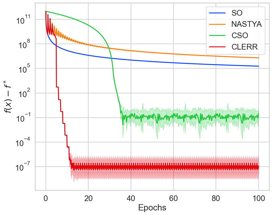
Figure 1: Function residual for (4), $\alpha_{t}=10^{-7}$.

We conduct this experiment on problem (4), where $d=1,\ N=1000$. We consider the Shuffle Once methods, which shuffle data once at the beginning of training. As baselines, we consider the following methods: regular SO method, which is just SGD with shuffling at the start of training, Nastya from Malinovsky et al. (2022) with one worker, Clipped SO (CSO), which clips stochastic gradients at every step of the method. The results are presented in Figure 1. As one can see from Figure 1, methods with clipping significantly outperform the rest. This empirical result justifies the theoretical fact of the importance of clipping for optimization of $(L_{0},L_{1})$-smooth objectives. Additionally, we see that among methods with clipping, CLERR shows better results than CSO. From this, we can conclude that clipping the final (pseudo)gradient approximation at the end of an epoch gives better results than clipping on every step.

5.1.1 ResNet-18 on CIFAR-10

In Zhang et al. (2020b) the authors obtained results on a positive correlation between gradient norm and local smoothness for the problem of training neural networks in language modeling and image classification tasks. To check, whether our findings in synthetic experiments also take place for neural networks, we decided to test Algorithm 2 in the same image classification problem: train ResNet-18 He et al. (2016) on the CIFAR-10 dataset Krizhevsky et al. (2009). Additionally, we consider heuristical modification of Algorithm 2, which we call CLERR-h. The details of it we provide next. The overall results of the experiment on test data are shown in Figure 2. Additionally, we provide results on train data along with technical details in Appendix F.

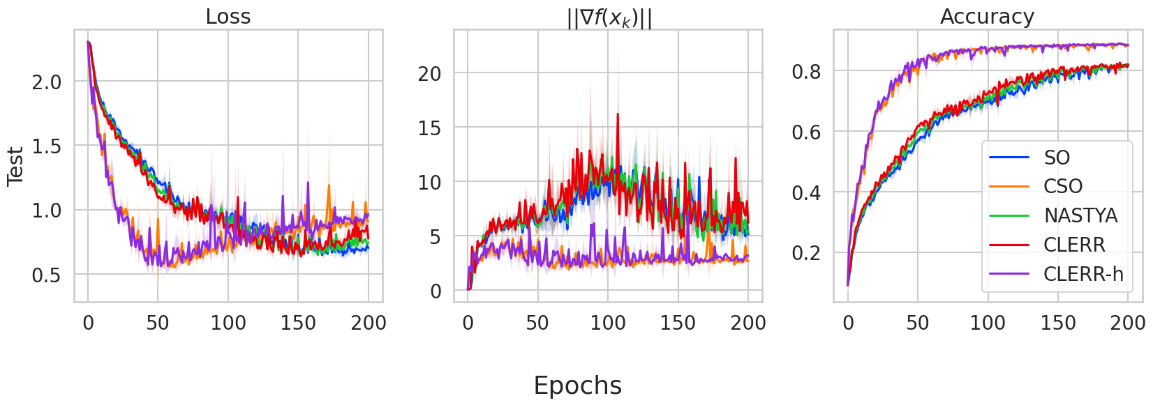
Figure 2: Loss, gradient norm and accuracy on test dataset for ResNet-18 on Cifar-10, $\alpha_{t}=0.01$

From this Figure we can see, that both jumping (Nastya and CLERR) and clipping on outer step (CLERR) does not have any impact on this problem. On the other hand, CSO shows the best results. Since in this problem regular clipping already works very well, we decided to heuristically modify our Algorithm 2: take the best clipping level and inner stepsize of CSO and use it on inner iterations, and tune $c_{0}$ with $c_{1}$ for outer stepsize. We call this method CLERR-h and also provide its results in Figure 2. CLERR-h chooses a rather big outer stepsize, while the outer clipping level is very tiny. For big clipping levels method diverges. These results show that jumping does not give performance gains when the method clips on every inner step.

5.2 Methods with local steps

In this experiment, we aim to show the effect of the jumping technique on federated learning methods. We consider problem (4) with $d=100,N=1000$. To make the distributions of data on each client more distinct between each other, we sort the whole dataset at the beginning of the experiment by $\|x_{i}\|$. Here we consider a high-dimensional setup so that the starting point has less impact on the algorithm performance. Indeed, in one-dimensional case, if we started from $x_{0}\not\in[-10,10]$, the anti-gradient of every $f_{i}(x)=(x-x_{i})^{4}$ would point towards minimum. Therefore, we could find such stepsize, that method converges in one iteration. On the other hand, if we consider a high-dimensional setup, then regardless of the starting point, the gradient of each $f_{i}(x)$ has a different direction. In this experiment we compare Algorithm 1 (C-LGDJ) with Communication Efficient Local Gradient Clipping (CELGC) (Liu et al., 2022) and Clipping-Enabled-FedAvg (CE-FedAvg) Zhang et al. (2022). The results are shown in Figure 3.

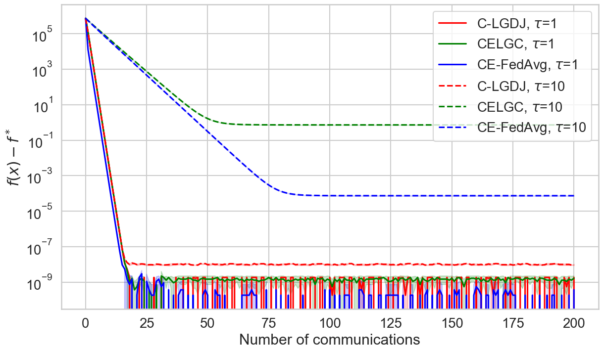
(a) $x_{0}=(1,...,1)$

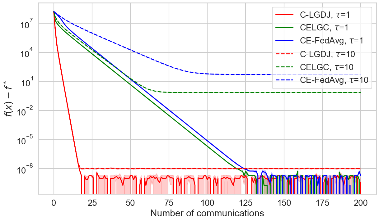
(b) $x_{0}=(10,...,10)$

Figure 3: Function residual for (4), starting from different $x_{0}$ for different number of local steps on the client device $\tau$.

Overall, we arrive at two conclusions. Firstly, local steps do not have any positive effect on this problem. The plots with the increased number of client steps $\tau$ only strengthen this point. Secondly, since local steps are pointless, the method works better if the server gets a better gradient approximation, which is true if the method clips gradients on the server, not on the client. This is exactly the reason why C-LGDJ has better performance in Figure 3(b).

5.3 Methods with local steps, random reshuffling and partial participation

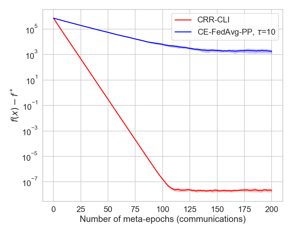
Figure 4: Function residual for (4), starting from $x_{0}=(1,...,1)$ with batch size 16.

In the final experiment, we consider methods with partial participation. The goal of this experiment is to investigate how clipping, local steps, partial participation and random reshuffling of both clients and client data works together. We compare Algorithm 3 with CE-FedAvg Zhang et al. (2022) with partial participation (CE-FedAvg-PP) on problem (4) with $d=100,N=1000$. Again, to make the distributions of data on each client more distinct between each other, we sort the whole dataset at the beginning of the experiment by $\|x_{i}\|$. The results are presented in Figure 4.

Since CRR-CLI uses random reshuffling of the data instead of sampling with replacement, and clips only in the end of meta-epoch, it has better gradient approximation on the global step, which results in better performance, than CE-FedAvg-PP.

6 Discussion

In this paper, we consider a more general smoothness assumption and propose three new distributed methods for Federated Learning with local steps under this setting. Specifically, we analyze local gradient descent (GD) steps, local steps with Random Reshuffling, and a method that combines local steps with Random Reshuffling and Partial Participation. We provide a tight analysis for general non-convex and Polyak-Łojasiewicz settings, recovering previous results as special cases. Furthermore, we present numerical results to support our theoretical findings.

For future work, it would be valuable to explore local methods with communication compression under the generalized smoothness assumption, as well as methods incorporating incomplete local epochs. Additionally, investigating local methods with client drift reduction mechanisms to address the effects of heterogeneity, along with potentially parameter-free approaches, represents a promising direction.

7 Acknowledgements

The research reported in this publication was supported by funding from King Abdullah University of Science and Technology (KAUST): i) KAUST Baseline Research Scheme, ii) Center of Excellence for Generative AI, under award number 5940, iii) SDAIA-KAUST Center of Excellence in Artificial Intelligence and Data Science.

Appendix A Implications of generalized smoothness

Lemma 1.

Let $f$ satisfy Assumption 2. Then, for any $x,y\in\mathbb{R}^{d}$ we have

$$f(y)\leq f(x)+\langle\nabla f(x),y-x\rangle+\frac{L_{0}+L_{1}\|\nabla f(x)\|}{2}\|x-y\|^{2}.$$

Moreover, if $f^{\star}:=\inf_{x\in\mathbb{R}^{d}}f(x)>-\infty$, then, for all $x\in\mathbb{R}^{d},$ we obtain

$$\frac{\|\nabla f(x)\|^{2}}{2(L_{0}+L_{1}\|\nabla f(x)\|)}\leq f(x)-f^{\star}.$$

Proof of Lemma 1.

The first statement of the lemma is proven in (Zhang et al., 2020b, Appendix A.1). The second statement is proven in (Gorbunov et al., 2024): it follows from the first statement, if one substitutes $y$ for $x-\frac{\left\lVert\nabla f(x)\right\rVert}{L_{0}+L_{1}\left\lVert\nabla f(x)\right\rVert}\nabla f(x)$ and uses the fact that $f^{\star}\leq f(y).$ ∎

Lemma 2.

Let $f$ satisfy Assumption 3. Then, for any $x,y\in\mathbb{R}^{d}$ we have

$$f(y)-f(x)\leq\langle\nabla f(x),y-x\rangle+\frac{L_{0}+L_{1}\|\nabla f(x)\|}{2}\exp(L_{1}\|x-y\|)\|x-y\|^{2}.$$

Moreover, if $f^{\star}:=\inf_{x\in\mathbb{R}^{d}}f(x)>-\infty$, then, for $\eta>0,$ such that $\eta\exp\eta\leq 1,$ for all $x\in\mathbb{R}^{d},$ we obtain

$$\frac{\eta\|\nabla f(x)\|^{2}}{2(L_{0}+L_{1}\|\nabla f(x)\|)}\leq f(x)-f^{\star}.$$

Proof of Lemma 2.

The first part of this lemma is one of the results of (Chen et al., 2023, Proposition 3.2). The second statement is proven in (Gorbunov et al., 2024). To deal with it, let us substitute $y$ in the first statement with $x-\frac{\eta\|\nabla f(x)\|}{L_{0}+L_{1}\|\nabla f(x)\|}\nabla f(x):$

$$f^{\star}\leq f(y) \leq f(x)+\langle\nabla f(x),y-x\rangle+\frac{L_{0}+L_{1}\|\nabla f(x)\|}{2}\exp(L_{1}\|x-y\|)\|x-y\|^{2}$$

$$=f(x)-\frac{\eta\|\nabla f(x)\|^{2}}{L_{0}+L_{1}\|\nabla f(x)\|}$$

$$+\frac{L_{0}+L_{1}\|\nabla f(x)\|}{2}\cdot\exp\left(\frac{L_{1}\eta\|\nabla f(x)\|}{L_{0}+L_{1}\|\nabla f(x)\|}\right)\cdot\frac{\eta^{2}\|\nabla f(x)\|^{2}}{(L_{0}+L_{1}\|\nabla f(x)\|)^{2}}$$

$$\leq f(x)-\frac{\eta\|\nabla f(x)\|^{2}}{L_{0}+L_{1}\|\nabla f(x)\|}+\frac{\eta\|\nabla f(x)\|^{2}}{2(L_{0}+L_{1}\|\nabla f(x)\|)}\cdot\eta\exp(\eta)$$

$$\leq f(x)-\frac{\eta\|\nabla f(x)\|^{2}}{2(L_{0}+L_{1}\|\nabla f(x)\|)}.$$

Rearranging the terms, we get the second statement of the lemma. ∎

Lemma 3.

Assumption 3 holds for the function $f$ if and only if, for any $x,y\in\mathbb{R}^{d},$

$$\left\lVert\nabla f(x)-\nabla f(y)\right\rVert\leq\left(L_{0}+L_{1}\left\lVert\nabla f(y)\right\rVert\right)\exp\left(L_{1}\left\lVert x-y\right\rVert\right)\left\lVert x-y\right\rVert.$$

Proof of Lemma 3.

This lemma is one of the results of (Chen et al., 2023, Proposition 3.2) ∎

Appendix B Local gradient descent

B.1 Asymmetric generalized-smooth non-convex functions

Theorem 1 (non-convex asymmetric generalized-smooth convergence analysis of Algorithm 1). Let Assumptions 1 and 2 hold for functions $f$ and $\left\{f_{m}\right\}_{m=1}^{M}$. Choose any $P\geq 1.$ For all $0\leq p\leq P-1,$ denote

$$\hat{a}_{p}=L_{0}+L_{1}\|\nabla f(\hat{x}_{t_{p}})\|,\quad a_{p}=L_{0}+L_{1}\max_{m}\|\nabla f_{m}(\hat{x}_{t_{p}})\|,\quad 1\leq t_{p+1}-t_{p}\leq H.$$

Put $\Delta^{\star}=f^{\star}-\frac{1}{M}\sum_{m=1}^{M}f_{m}^{\star}.$ Impose the following conditions on the local stepsizes $\alpha_{p}$ and server stepsizes $\gamma_{p}:$

$$\alpha_{p}\leq\min\left\{\frac{1}{2Ha_{p}},\frac{1}{ca_{p}}\sqrt{\frac{\hat{a}_{p}}{a_{p}}}\right\},\quad\frac{\zeta}{\hat{a}_{p}}\leq\gamma_{p}\leq\frac{1}{4\hat{a}_{p}},\quad 0\leq p\leq P-1,$$

where $0<\zeta\leq\frac{1}{4},$ $c\geq\sqrt{P}.$ Let $\delta_{0}\overset{\text{def}}{=}f\left(x_{0}\right)-f^{\star}.$ Then, the iterates $\left\{\hat{x}_{t_{p}}\right\}_{p=0}^{P-1}$ of Algorithm 1 satisfy

$$\min_{0\leq p\leq P-1}\left\{\frac{\zeta}{8}\min\left\{\frac{\|\nabla f(\hat{x}_{t_{p}})\|^{2}}{L_{0}},\frac{\|\nabla f(\hat{x}_{t_{p}})\|}{L_{1}}\right\}\right\} \leq\frac{\left(1+\frac{3(H-1)\alpha_{p}^{2}a_{p}^{3}}{2\hat{a}_{p}}\right)^{P}}{P}\delta_{0}$$

$$+\frac{3(H-1)\alpha_{p}^{2}a_{p}^{3}}{2\hat{a}_{p}}\Delta^{\star}.$$

Put $v_{p}\overset{\text{def}}{=}t_{p+1}-1.$

Lemma 4.

Assume that $f$ and each $f_{m}$ satisfy Assumptions 1 and 2. Then we have the following bound:

$$\frac{1}{M}\sum_{m=1}^{M}\sum_{t=t_{p}+1}^{v}\left\lVert x_{t}^{m}-\hat{x}_{t_{p}}\right\rVert^{2}\leq 8\left(v_{p}-t_{p}\right)^{2}a_{p}\alpha_{p}^{2}\left(f(\hat{x}_{t_{p}})-f^{\star}+\Delta^{\star}\right).$$

Proof of Lemma 4.

We have

$$\left\lVert x_{t}^{m}-\hat{x}_{t_{p}}\right\rVert^{2} =\left\lVert\sum_{j=t_{p}}^{t-1}\alpha_{p}\nabla f_{m}\left(x_{j}^{m}\right)\right\rVert^{2}$$

$$\leq 2\left\|\sum_{j=t_{p}}^{t-1}\alpha_{p}\left(\nabla f_{m}(x_{j}^{m})-\nabla f_{m}(\hat{x}_{t_{p}})\right)\right\|^{2}+2\left\|\sum_{j=t_{p}}^{t-1}\alpha_{p}\nabla f_{m}(\hat{x}_{t_{p}})\right\|^{2}$$

$$\leq 2(t-t_{p})\sum_{j=t_{p}}^{t-1}\left(\alpha_{p}\right)^{2}\left(L_{0}+L_{1}\left\lVert\nabla f_{m}(\hat{x}_{t_{p}})\right\rVert\right)^{2}\left\lVert x_{j}^{m}-\hat{x}_{t_{p}}\right\rVert^{2}$$

$$+2\left\|\sum_{j=t_{p}}^{t-1}\alpha_{p}\nabla f_{m}(\hat{x}_{t_{p}})\right\|^{2}.$$

Averaging, we get

$$\frac{1}{M}\sum_{m=1}^{M}\left\lVert x_{t}^{m}-\hat{x}_{t_{p}}\right\rVert^{2} \leq\frac{2(t-t_{p})}{M}\sum_{m=1}^{M}\sum_{j=t_{p}}^{t-1}\left(\alpha_{p}\right)^{2}\left(L_{0}+L_{1}\left\lVert\nabla f_{m}(\hat{x}_{t_{p}})\right\rVert\right)^{2}\left\lVert x_{j}^{m}-\hat{x}_{t_{p}}\right\rVert^{2}$$

$$+\frac{2}{M}\sum_{m=1}^{M}\left\|\sum_{j=t_{p}}^{t-1}\alpha_{p}\nabla f_{m}(\hat{x}_{t_{p}})\right\|^{2}$$

$$\leq\frac{2(t-t_{p})}{M}\left(a_{p}\right)^{2}\sum_{m=1}^{M}\sum_{j=t_{p}}^{t-1}\left(\alpha_{p}\right)^{2}\left\lVert x_{j}^{m}-\hat{x}_{t_{p}}\right\rVert^{2}$$

$$+\frac{2}{M}\sum_{m=1}^{M}\left\|\sum_{j=t_{p}}^{t-1}\alpha_{p}\nabla f_{m}(\hat{x}_{t_{p}})\right\|^{2}.$$

Recall that $\alpha_{p}\leq\frac{1}{2H\left(L_{0}+L_{1}\max_{m}\left\lVert\nabla f_{m}(\hat{x}_{t_{p}})\right\rVert\right)}.$ Then we have

$$\frac{1}{M}\sum_{m=1}^{M}\left\lVert x_{t}^{m}-\hat{x}_{t_{p}}\right\rVert^{2} \leq\frac{t-t_{p}}{2H^{2}M}\sum_{m=1}^{M}\sum_{j=t_{p}}^{t-1}\left\lVert x_{j}^{m}-\hat{x}_{t_{p}}\right\rVert^{2}$$

$$+\frac{2}{M}\sum_{m=1}^{M}\left\|\sum_{j=t_{p}}^{t-1}\alpha_{p}\nabla f_{m}(\hat{x}_{t_{p}})\right\|^{2}.$$ (5)

Let us bound the last term:

$$\frac{2}{M}\sum_{m=1}^{M}\left\|\sum_{j=t_{p}}^{t-1}\alpha_{p}\nabla f_{m}(\hat{x}_{t_{p}})\right\|^{2} \leq\frac{2}{M}\sum_{m=1}^{M}\left\lVert\nabla f_{m}(\hat{x}_{t_{p}})\right\rVert^{2}\left(t-t_{p}\right)^{2}\alpha_{p}^{2}$$

$$\leq\frac{4}{M}\sum_{m=1}^{M}\left(L_{0}+L_{1}\left\lVert\nabla f_{m}(\hat{x}_{t_{p}})\right\rVert\right)\left(f_{m}\left(\hat{x}_{t_{p}}\right)-f_{m}^{\star}\right)$$

$$\times\left(t-t_{p}\right)^{2}\alpha_{p}^{2}$$

$$\leq\frac{4\left(t-t_{p}\right)^{2}a_{p}\alpha_{p}^{2}}{M}\sum_{m=1}^{M}\left(f_{m}\left(\hat{x}_{t_{p}}\right)-f_{m}^{\star}\right)$$

$$=4\left(t-t_{p}\right)^{2}a_{p}\alpha_{p}^{2}\left(f(\hat{x}_{t_{p}})-f^{\star}+\left(f^{\star}-\frac{1}{M}\sum_{m=1}^{M}f_{m}^{\star}\right)\right)p$$

$$=4\left(t-t_{p}\right)^{2}a_{p}\alpha_{p}^{2}\left(f(\hat{x}_{t_{p}})-f^{\star}+\Delta^{\star}\right).$$

Further, summing (7) with respect to $t,$ we obtain

$$\frac{1}{M}\sum_{m=1}^{M}\sum_{t=t_{p}+1}^{v}\left\lVert x_{t}^{m}-\hat{x}_{t_{p}}\right\rVert^{2} \leq\frac{1}{2H^{2}M}\sum_{m=1}^{M}\sum_{t=t_{p}+1}^{v}(t-t_{p})\sum_{j=t_{p}}^{t-1}\left\lVert x_{j}^{m}-\hat{x}_{t_{p}}\right\rVert^{2}$$

$$+\sum_{t=t_{p}+1}^{v}4\left(t-t_{p}\right)^{2}a_{p}\alpha_{p}^{2}\left(f(\hat{x}_{t_{p}})-f^{\star}+\Delta^{\star}\right)$$

$$\leq\frac{v-t_{p}}{2H^{2}M}\sum_{m=1}^{M}\sum_{t=t_{p}+1}^{v}\sum_{j=t_{p}}^{v}\left\lVert x_{j}^{m}-\hat{x}_{t_{p}}\right\rVert^{2}$$

$$+4\sum_{t=t_{p}+1}^{v}\left(v-t_{p}\right)^{2}a_{p}\alpha_{p}^{2}\left(f(\hat{x}_{t_{p}})-f^{\star}+\Delta^{\star}\right)$$

$$\leq\frac{\left(v-t_{p}\right)^{2}}{2H^{2}M}\sum_{m=1}^{M}\sum_{j=t_{p}}^{v}\left\lVert x_{j}^{m}-\hat{x}_{t_{p}}\right\rVert^{2}$$

$$+4\left(v-t_{p}\right)^{3}a_{p}\alpha_{p}^{2}\left(f(\hat{x}_{t_{p}})-f^{\star}+\Delta^{\star}\right).$$

Using the fact that $v-t_{p}\leq H-1<H,$ we obtain that

$$\frac{1}{M}\sum_{m=1}^{M}\sum_{t=t_{p}+1}^{v}\left\lVert x_{t}^{m}-\hat{x}_{t_{p}}\right\rVert^{2}\leq 8\left(v-t_{p}\right)^{3}a_{p}\alpha_{p}^{2}\left(f(\hat{x}_{t_{p}})-f^{\star}+\Delta^{\star}\right).$$

∎

Proof of Theorem 1.

Applying Lemma 1, we obtain that

$$f(\hat{x}_{t_{p+1}})\leq f(\hat{x}_{t_{p}})-\gamma_{p}\langle\nabla f\left(\hat{x}_{t_{p}}\right),g_{p}\rangle+\left(L_{0}+L_{1}\left\lVert\nabla f\left(\hat{x}_{t_{p}}\right)\right\rVert\right)\frac{\gamma_{p}^{2}\left\lVert g_{p}\right\rVert^{2}}{2}.$$

Additionally, from the fact that $2\langle a,b\rangle=-\|a-b\|^{2}+\|a\|^{2}+\|b\|^{2}$

$$f(\hat{x}_{t_{p+1}}) \leq f(\hat{x}_{t_{p}})-\gamma_{p}\langle\nabla f\left(\hat{x}_{t_{p}}\right),g_{p}\rangle+\left(L_{0}+L_{1}\left\lVert\nabla f\left(\hat{x}_{t_{p}}\right)\right\rVert\right)\frac{\gamma_{p}^{2}\left\lVert g_{p}\right\rVert^{2}}{2}$$

$$\leq f(\hat{x}_{t_{p}})-\frac{\gamma_{p}}{2}(-\|\nabla f(\hat{x}_{t_{p}})-g_{p}\|^{2}+\|\nabla f(x_{p})\|^{2}+\|g_{p}\|^{2})$$

$$+(L_{0}+L_{1}\|\nabla f(\hat{x}_{t_{p}})\|)\frac{\gamma_{p}^{2}\|g_{p}\|^{2}}{2}$$

$$\leq f(\hat{x}_{t_{p}})-\frac{\gamma_{p}}{2}\|\nabla f(\hat{x}_{t_{p}})\|^{2}+\frac{\gamma_{p}}{2}\|\nabla f(\hat{x}_{t_{p}})-g_{p}\|^{2}+(L_{0}+L_{1}\|\nabla f(\hat{x}_{t_{p}})\|)\frac{\gamma_{p}^{2}\|g_{p}\|^{2}}{2}.$$

Consider $\frac{\gamma_{p}}{2}\|\nabla f(\hat{x}_{t_{p}})-g_{p}\|^{2}.$ We have

$$\frac{\gamma_{p}}{2}\|\nabla f(\hat{x}_{t_{p}})-g_{p}\|^{2} =\frac{\gamma_{p}}{2}\left\|\frac{1}{M}\sum_{m=1}^{M}\left(\nabla f_{m}(\hat{x}_{t_{p}})-\frac{1}{v-t_{p}}\sum_{j=t_{p}}^{v}\nabla f_{m}\left(x_{j}^{m}\right)\right)\right\|^{2}$$

$$\leq\frac{\gamma_{p}}{2}\frac{1}{M(v-t_{p})^{2}}\sum_{m=1}^{M}(L_{0}+L_{1}\|\nabla f_{m}(\hat{x}_{t_{p}})\|)^{2}\sum_{j=t_{p}}^{v}\|x_{j}^{m}-\hat{x}_{t_{p}}\|^{2}$$

$$\leq\frac{\gamma_{p}}{2(v-t_{p})^{2}}(L_{0}+L_{1}\max_{m}\|\nabla f_{m}(\hat{x}_{t_{p}})\|)^{2}\frac{1}{M}\sum_{m=1}^{M}\sum_{j=t_{p}}^{v}\|x_{j}^{m}-\hat{x}_{t_{p}}\|^{2}$$

$$=\frac{\gamma_{p}a_{p}^{2}}{2(v-t_{p})^{2}}\frac{1}{M}\sum_{m=1}^{M}\sum_{j=t_{p}}^{v}\|x_{j}^{m}-\hat{x}_{t_{p}}\|^{2}.$$

Notice that

$$\frac{\gamma_{p}^{2}\left\lVert g_{p}\right\rVert^{2}}{2} =\frac{\gamma_{p}^{2}}{2}\left\lVert\frac{1}{M(v-t_{p})}\sum_{m=1}^{M}\sum_{j=t_{p}+1}^{v}\nabla f_{m}\left(x_{j}^{m}\right)\right\rVert^{2}$$

$$\leq\frac{\gamma_{p}^{2}}{(v-t_{p})^{2}}\left\lVert\frac{1}{M}\sum_{m=1}^{M}\sum_{j=t_{p}+1}^{v}\left(\nabla f_{m}\left(x_{j}^{m}\right)-\nabla f_{m}\left(\hat{x}_{t_{p}}\right)\right)\right\rVert^{2}$$

$$+\frac{\gamma_{p}^{2}}{(v-t_{p})^{2}}\left\lVert\frac{1}{M}\sum_{m=1}^{M}\sum_{j=t_{p}+1}^{v}\nabla f_{m}\left(\hat{x}_{t_{p}}\right)\right\rVert^{2}$$

$$\leq\frac{\gamma_{p}^{2}}{(v-t_{p})^{2}}\left(L_{0}+L_{1}\max_{m}\left\lVert\nabla f_{m}(\hat{x}_{t_{p}})\right\rVert\right)^{2}\frac{1}{M}\sum_{m=1}^{M}\sum_{j=t_{p}}^{v}\left\lVert x_{j}^{m}-\hat{x}_{t_{p}}\right\rVert^{2}$$

$$+\gamma_{p}^{2}\left\lVert\nabla f\left(\hat{x}_{t_{p}}\right)\right\rVert^{2}$$

$$=\frac{\gamma_{p}^{2}a_{p}^{2}}{M(v-t_{p})^{2}}\sum_{m=1}^{M}\sum_{j=t_{p}}^{v}\left\lVert x_{j}^{m}-\hat{x}_{t_{p}}\right\rVert^{2}+\gamma_{p}^{2}\left\lVert\nabla f\left(\hat{x}_{t_{p}}\right)\right\rVert^{2}.$$

Therefore, we obtain

$$f\left(\hat{x}_{t_{p+1}}\right) \leq f(\hat{x}_{t_{p}})-\frac{\gamma_{p}}{2}\|\nabla f(\hat{x}_{t_{p}})\|^{2}+\frac{\gamma_{p}a_{p}^{2}}{2M(v-t_{p})^{2}}\sum_{m=1}^{M}\sum_{j=t_{p}}^{v}\|x_{j}^{m}-\hat{x}_{t_{p}}\|^{2}+\frac{\hat{a}_{p}\gamma_{p}^{2}\|g_{p}\|^{2}}{2}$$

$$\leq f(\hat{x}_{t_{p}})-\frac{\gamma_{p}}{2}\|\nabla f(\hat{x}_{t_{p}})\|^{2}+\frac{\gamma_{p}a_{p}^{2}}{2M(v-t_{p})^{2}}\sum_{m=1}^{M}\sum_{j=t_{p}}^{v}\|x_{j}^{m}-\hat{x}_{t_{p}}\|^{2}$$

$$+\frac{\hat{a}_{p}a_{p}^{2}\gamma_{p}^{2}}{M(v-t_{p})^{2}}\sum_{m=1}^{M}\sum_{j=t_{p}}^{v}\left\lVert x_{j}^{m}-\hat{x}_{t_{p}}\right\rVert^{2}+\hat{a}_{p}\gamma_{p}^{2}\left\lVert\nabla f\left(\hat{x}_{t_{p}}\right)\right\rVert^{2}$$

$$=f(\hat{x}_{t_{p}})+\left(\hat{a}_{p}\gamma_{p}^{2}-\frac{\gamma_{p}}{2}\right)\left\lVert\nabla f\left(\hat{x}_{t_{p}}\right)\right\rVert^{2}$$

$$+\left(\hat{a}_{p}a_{p}^{2}\gamma_{p}^{2}+\frac{\gamma_{p}a_{p}^{2}}{2}\right)\frac{1}{M(v-t_{p})^{2}}\sum_{m=1}^{M}\sum_{j=t_{p}}^{v}\left\lVert x_{j}^{m}-\hat{x}_{t_{p}}\right\rVert^{2}.$$

Recall that $\gamma_{p}\leq\frac{1}{4\hat{a}_{p}}.$ Then, using Lemma 4, we have

$$f\left(\hat{x}_{t_{p+1}}\right) \leq f\left(\hat{x}_{t_{p}}\right)-\frac{\gamma_{p}}{4}\left\lVert\nabla f\left(\hat{x}_{t_{p}}\right)\right\rVert^{2}$$

$$+\left(\hat{a}_{p}a_{p}^{2}\gamma_{p}^{2}+\frac{\gamma_{p}a_{p}^{2}}{2}\right)\frac{1}{M(v-t_{p})^{2}}\sum_{m=1}^{M}\sum_{j=t_{p}}^{v}\left\lVert x_{j}^{m}-\hat{x}_{t_{p}}\right\rVert^{2}$$

$$\leq f\left(\hat{x}_{t_{p}}\right)-\frac{\gamma_{p}}{4}\left\lVert\nabla f\left(\hat{x}_{t_{p}}\right)\right\rVert^{2}$$

$$+\left(\hat{a}_{p}a_{p}^{2}\gamma_{p}^{2}+\frac{\gamma_{p}a_{p}^{2}}{2}\right)8(v-t_{p})a_{p}\alpha_{p}^{2}\left(f(\hat{x}_{t_{p}})-f^{\star}+\Delta^{\star}\right)$$

$$\leq f\left(\hat{x}_{t_{p}}\right)-\frac{\gamma_{p}}{4}\left\lVert\nabla f\left(\hat{x}_{t_{p}}\right)\right\rVert^{2}+\frac{3(H-1)a_{p}^{3}\alpha_{p}^{2}\left(f(\hat{x}_{t_{p}})-f^{\star}+\Delta^{\star}\right)}{2\hat{a}_{p}}.$$

Let us rewrite the inequality in the following way:

$$\frac{\gamma_{p}}{4}\left\lVert\nabla f\left(\hat{x}_{t_{p}}\right)\right\rVert^{2}\leq f\left(\hat{x}_{t_{p}}\right)-f\left(\hat{x}_{t_{p+1}}\right)+\frac{3(H-1)a_{p}^{3}\alpha_{p}^{2}\left(f(\hat{x}_{t_{p}})-f^{\star}+\Delta^{\star}\right)}{2\hat{a}_{p}}.$$ (6)

Since $\gamma_{p}\geq\frac{\zeta}{\hat{a}_{p}},$ we get that

$$\frac{\gamma_{p}\left\lVert\nabla f\left(\hat{x}_{t_{p}}\right)\right\rVert^{2}}{4}\geq\frac{\zeta\left\lVert\nabla f\left(\hat{x}_{t_{p}}\right)\right\rVert^{2}}{4\hat{a}_{p}}.$$

Therefore,

$$\frac{\gamma_{p}}{4}\|\nabla f(\hat{x}_{t_{p}})\|^{2}\geq\begin{cases}\frac{\zeta\|\nabla f(\hat{x}_{t_{p}})\|^{2}}{8L_{0}},&\|\nabla f(\hat{x}_{t_{p}})\|\leq\frac{L_{0}}{L_{1}},\\ \frac{\zeta\|\nabla f(\hat{x}_{t_{p}})\|}{8L_{1}},&\|\nabla f(\hat{x}_{t_{p}})\|>\frac{L_{0}}{L_{1}},\end{cases}=\frac{\zeta}{8}\min\left\{\frac{\|\nabla f(\hat{x}_{t_{p}})\|^{2}}{L_{0}},\frac{\|\nabla f(\hat{x}_{t_{p}})\|}{L_{1}}\right\}.$$

Denote $\delta_{p}\overset{\text{def}}{=}f\left(\hat{x}_{t_{p}}\right)-f^{\star}.$ Then we have

$$\frac{\zeta}{8}\min\left\{\frac{\|\nabla f(\hat{x}_{t_{p}})\|^{2}}{L_{0}},\frac{\|\nabla f(\hat{x}_{t_{p}})\|}{L_{1}}\right\}\leq\delta_{p}-\delta_{p+1}+\frac{3(H-1)\alpha_{p}^{2}a_{p}^{3}\left(\delta_{p}+\Delta^{\star}\right)}{2\hat{a}_{p}}.$$

Let $\alpha_{p}\leq\frac{1}{ca_{p}}\sqrt{\frac{\hat{a}_{p}}{a_{p}}},$ where $c\geq\sqrt{P}.$ Applying the result of Mishchenko et al. (2020, Lemma 6), we appear at

$$\min_{0\leq p\leq P-1}\left\{\frac{\zeta}{8}\min\left\{\frac{\|\nabla f(\hat{x}_{t_{p}})\|^{2}}{L_{0}},\frac{\|\nabla f(\hat{x}_{t_{p}})\|}{L_{1}}\right\}\right\} \leq\frac{\left(1+\frac{3(H-1)\alpha_{p}^{2}a_{p}^{3}}{2\hat{a}_{p}}\right)^{P}}{P}\delta_{0}$$

$$+\frac{3(H-1)\alpha_{p}^{2}a_{p}^{3}}{2\hat{a}_{p}}\Delta^{\star}.$$

∎

Corollary 1. Fix $\varepsilon>0.$ Choose $c=\sqrt{3(H-1)P}.$ Let $\alpha_{p}\leq 2\sqrt{\frac{\hat{a}_{p}\delta_{0}}{3P(H-1)a_{p}^{3}\Delta^{\star}}}.$ Then, if $P\geq\frac{32\delta_{0}}{\zeta\varepsilon},$ we have $\min_{0\leq p\leq P-1}\left\{\min\left\{\frac{\|\nabla f(\hat{x}_{t_{p}})\|^{2}}{L_{0}},\frac{\|\nabla f(\hat{x}_{t_{p}})\|}{L_{1}}\right\}\right\}\leq\varepsilon.$

Proof of Corollary 1.

Since $c=\sqrt{3(H-1)P}$ and $\alpha_{p}\leq\frac{1}{ca_{p}}\sqrt{\frac{\hat{a}_{p}}{a_{p}}},$ $\alpha_{p}\leq 2\sqrt{\frac{\hat{a}_{p}\delta_{0}}{3P(H-1)a_{p}^{3}\Delta^{\star}}},$ due to the choice of $P\geq\frac{32\delta_{0}}{\zeta\varepsilon},$ we obtain that

$$\frac{\left(1+\frac{3(H-1)\alpha_{p}^{2}a_{p}^{3}}{2\hat{a}_{p}}\right)^{P}}{P}\delta_{0}\leq\frac{\sqrt{e}\delta_{0}}{P}\leq\frac{2\delta_{0}}{P}\leq\frac{\zeta\varepsilon}{16},$$

and that

$$\frac{3(H-1)\alpha_{p}^{2}a_{p}^{3}}{2\hat{a}_{p}}\Delta^{\star}\leq\frac{\zeta\varepsilon}{16}.$$

Therefore, $\min_{0\leq p\leq P-1}\left\{\min\left\{\frac{\|\nabla f(\hat{x}_{t_{p}})\|^{2}}{L_{0}},\frac{\|\nabla f(\hat{x}_{t_{p}})\|}{L_{1}}\right\}\right\}\leq\varepsilon.$ ∎

B.2 Asymmetric generalized-smooth functions under PŁ-condition

Theorem 2 (Asymmetric generalized-smooth convergence analysis of Algorithm 1 in PŁ-case). Let Assumptions 1 and 2 hold for functions $f$ and $\left\{f_{m}\right\}_{m=1}^{M}.$ Let Assumption 4 hold. Choose $0<\zeta\leq\frac{1}{4}.$ Let $\delta_{0}\overset{\text{def}}{=}f\left(x_{0}\right)-f^{\star}.$ Choose any integer $P>\frac{64\delta_{0}L_{1}^{2}}{\mu\zeta}.$ For all $0\leq p\leq P-1,$ denote

$$\hat{a}_{p}=L_{0}+L_{1}\|\nabla f(\hat{x}_{t_{p}})\|,\quad a_{p}=L_{0}+L_{1}\max_{m}\|\nabla f_{m}(\hat{x}_{t_{p}})\|,\quad 1\leq t_{p+1}-t_{p}\leq H.$$

Put $\Delta^{\star}=f^{\star}-\frac{1}{M}\sum_{m=1}^{M}f_{m}^{\star}.$ Impose the following conditions on the local stepsizes $\alpha_{p}$ and server stepsizes $\gamma_{p}:$

$$\alpha_{p}\leq\min\left\{\frac{1}{2Ha_{p}},\frac{1}{ca_{p}}\sqrt{\frac{\hat{a}_{p}}{a_{p}}},\sqrt{\frac{\mu\zeta\hat{a}_{p}}{48L_{1}^{2}(H-1)a_{p}^{3}\left(f(\hat{x}_{t_{p}})-f^{\star}+\Delta^{\star}\right)}},\right.\\ \left.\sqrt{\frac{2\delta_{0}\hat{a}_{p}}{3P(H-1)a_{p}^{3}\left(f(\hat{x}_{t_{p}})-f^{\star}+\Delta^{\star}\right)}}\right\},$$

$$\frac{\zeta}{\hat{a}_{p}}\leq\gamma_{p}\leq\frac{1}{4\hat{a}_{p}},\quad 0\leq p\leq P-1,$$

where $c\geq\sqrt{P}.$ Let $\tilde{P}$ be an integer such that $0\leq\tilde{P}\leq\frac{64\delta_{0}L_{1}^{2}}{\mu\zeta},$ $A>0$ be a constant, $\alpha\leq\sqrt{\frac{\delta_{0}}{AP}}.$ Then, the iterates $\left\{\hat{x}_{t_{p}}\right\}_{p=0}^{P}$ of Algorithm 1 satisfy

$$\delta_{P}\leq\left(1-\frac{\mu\zeta}{4L_{0}}\right)^{P-\tilde{P}}\delta_{0}+\frac{4L_{0}A\alpha^{2}}{\mu\zeta},$$

where $\delta_{P}\overset{\text{def}}{=}f\left(\hat{x}_{t_{P}}\right)-f^{\star}.$

Proof of Theorem 2.

Let us follow the first steps of the proof of Theorem 1. Consider (6):

$$\frac{\gamma_{p}}{4}\left\lVert\nabla f\left(\hat{x}_{t_{p}}\right)\right\rVert^{2}\leq f\left(\hat{x}_{t_{p}}\right)-f\left(\hat{x}_{t_{p+1}}\right)+\frac{3(H-1)a_{p}^{3}\alpha_{p}^{2}\left(f(\hat{x}_{t_{p}})-f^{\star}+\Delta^{\star}\right)}{2\hat{a}_{p}}.$$

Since $\gamma_{p}\geq\frac{\zeta}{\hat{a}_{p}},$ and $f$ satisfies Polyak–Łojasiewicz Assumption 4, we obtain that

$$\frac{\mu\zeta\left(f(\hat{x}_{t_{p}})-f^{\star}\right)}{2\hat{a}_{p}}\leq f\left(\hat{x}_{t_{p}}\right)-f\left(\hat{x}_{t_{p+1}}\right)+\frac{3(H-1)a_{p}^{3}\alpha_{p}^{2}\left(f(\hat{x}_{t_{p}})-f^{\star}+\Delta^{\star}\right)}{2\hat{a}_{p}}.$$

1. Let $\tilde{P}$ be the number of steps $p,$ so that $\left\lVert\nabla f\left(\hat{x}_{t_{p}}\right)\right\rVert\geq\frac{L_{0}}{L_{1}}.$ For such $p,$ we have $L_{0}+L_{1}\left\lVert\nabla f\left(\hat{x}_{t_{p}}\right)\right\rVert=\hat{a}_{p}\leq 2L_{1}\left\lVert\nabla f\left(\hat{x}_{t_{p}}\right)\right\rVert.$ Therefore, we get

$$\frac{\mu\zeta\left(f(\hat{x}_{t_{p}})-f^{\star}\right)}{4L_{1}\left\lVert\nabla f\left(\hat{x}_{t_{p}}\right)\right\rVert}\leq f\left(\hat{x}_{t_{p}}\right)-f\left(\hat{x}_{t_{p+1}}\right)+\frac{3(H-1)a_{p}^{3}\alpha_{p}^{2}\left(f(\hat{x}_{t_{p}})-f^{\star}+\Delta^{\star}\right)}{2\hat{a}_{p}}.$$

Notice that the relation $\hat{a}_{p}\leq 2L_{1}\left\lVert\nabla f\left(\hat{x}_{t_{p}}\right)\right\rVert$ and Lemma 1 together imply

$$\frac{\left\lVert\nabla f\left(\hat{x}_{t_{p}}\right)\right\rVert}{4L_{1}}\leq\frac{{\left\lVert\nabla f\left(\hat{x}_{t_{p}}\right)\right\rVert}^{2}}{2\hat{a}_{p}}\leq f\left(\hat{x}_{t_{p}}\right)-f^{\star}.$$

Hence, we have

$$\frac{\mu\zeta}{16L_{1}^{2}}\leq f\left(\hat{x}_{t_{p}}\right)-f\left(\hat{x}_{t_{p+1}}\right)+\frac{3(H-1)a_{p}^{3}\alpha_{p}^{2}\left(f(\hat{x}_{t_{p}})-f^{\star}+\Delta^{\star}\right)}{2\hat{a}_{p}}.$$

Subtracting $f^{\star}$ on both sides and introducing $\delta_{p}\overset{\text{def}}{=}f\left(\hat{x}_{t_{p}}\right)-f^{\star},$ we obtain

$$\delta_{p+1}\leq\delta_{p}-\frac{\mu\zeta}{16L_{1}^{2}}+\frac{3(H-1)a_{p}^{3}\alpha_{p}^{2}\left(f(\hat{x}_{t_{p}})-f^{\star}+\Delta^{\star}\right)}{2\hat{a}_{p}}.$$

As $\alpha_{p}\leq\sqrt{\frac{\mu\zeta\hat{a}_{p}}{48L_{1}^{2}(H-1)a_{p}^{3}\left(f(\hat{x}_{t_{p}})-f^{\star}+\Delta^{\star}\right)}},$ it follows that $\frac{3(H-1)a_{p}^{3}\alpha_{p}^{2}\left(f(\hat{x}_{t_{p}})-f^{\star}+\Delta^{\star}\right)}{2\hat{a}_{p}}\leq\frac{\mu\zeta}{32L_{1}^{2}}.$ Therefore, we get

$$\delta_{p+1}\leq\delta_{p}-\frac{\mu\zeta}{32L_{1}^{2}}.$$

2. Suppose now that $\left\lVert\nabla f\left(\hat{x}_{t_{p}}\right)\right\rVert\leq\frac{L_{0}}{L_{1}}.$ For such $p,$ we have $L_{0}+L_{1}\left\lVert\nabla f\left(\hat{x}_{t_{p}}\right)\right\rVert=\hat{a}_{p}\leq 2L_{0}.$ Hence,

$$\frac{\mu\zeta\left(f(\hat{x}_{t_{p}})-f^{\star}\right)}{4L_{0}}\leq f\left(\hat{x}_{t_{p}}\right)-f\left(\hat{x}_{t_{p+1}}\right)+\frac{3(H-1)a_{p}^{3}\alpha_{p}^{2}\left(f(\hat{x}_{t_{p}})-f^{\star}+\Delta^{\star}\right)}{2\hat{a}_{p}}.$$

Subtracting $f^{\star}$ on both sides and introducing $\delta_{p}\overset{\text{def}}{=}f\left(\hat{x}_{t_{p}}\right)-f^{\star},$ we obtain

$$\delta_{p+1}\leq\delta_{p}\rho+\frac{3(H-1)a_{p}^{3}\alpha_{p}^{2}\left(f(\hat{x}_{t_{p}})-f^{\star}+\Delta^{\star}\right)}{2\hat{a}_{p}},\quad\text{ where }\rho\overset{\text{def}}{=}1-\frac{\mu\zeta}{4L_{0}}.$$

Let $\alpha_{p}\overset{\text{def}}{=}\alpha\hat{\alpha}_{p}$ and $\hat{\alpha}_{p}\leq\sqrt{\frac{2A\hat{a}_{p}}{3(H-1)a_{p}^{3}\left(f(\hat{x}_{t_{p}})-f^{\star}+\Delta^{\star}\right)}}$ for some constant $A>0.$ Then,

$$\delta_{p+1}\leq\rho\delta_{p}+A\alpha^{2}.$$

Unrolling the recursion, we derive

$$\delta_{P} \leq\rho^{P-\tilde{P}}\delta_{0}+A\alpha^{2}\sum_{i=0}^{\infty}\rho^{i}-\frac{\mu\zeta}{32L_{1}^{2}}\sum_{i=0}^{N-1}\rho^{i}$$

$$\leq\rho^{P-\tilde{P}}\delta_{0}+\frac{A\alpha^{2}}{1-\rho}-\frac{1-\rho^{\tilde{P}}}{1-\rho}\frac{\mu\zeta}{32L_{1}^{2}}.$$

Notice that $\delta_{p+1}\leq\delta_{p}+A\alpha^{2},$ which implies

$$\delta_{P}\leq\delta_{0}+\left(P-\tilde{P}\right)A\alpha^{2}-\tilde{P}\frac{\mu\zeta}{32L_{1}^{2}}.$$

Since $\alpha\leq\sqrt{\frac{\delta_{0}}{AP}},$ we conclude that

$$0\leq\delta_{P}\leq 2\delta_{0}-\tilde{P}\frac{\mu\zeta}{32L_{1}^{2}},\quad\Rightarrow\tilde{P}\leq\frac{64\delta_{0}L_{1}^{2}}{\mu\zeta}.$$

Therefore, for $P>\frac{64\delta_{0}L_{1}^{2}}{\mu\zeta}$ we can guarantee that $P-\tilde{P}>0$ and

$$\delta_{P} \leq\rho^{P-\tilde{P}}\delta_{0}+\frac{A\alpha^{2}}{1-\rho}-\tilde{P}\rho^{\tilde{P}}\frac{\mu\zeta}{32L_{1}^{2}}$$

$$\leq\rho^{P-\tilde{P}}\delta_{0}+\frac{A\alpha^{2}}{1-\rho}.$$

∎

Corollary 2. Fix $\varepsilon>0.$ Choose $\alpha\leq\min\left\{\sqrt{\frac{\delta_{0}}{AP}},L_{1}\sqrt{\frac{8\delta_{0}\varepsilon}{L_{0}AP}}\right\}.$ Then, if $P\geq\frac{64\delta_{0}L_{1}^{2}}{\mu\zeta}+\frac{4L_{0}}{\mu\zeta}\ln\frac{2\delta_{0}}{\varepsilon},$ we have $\delta_{P}\leq\varepsilon.$

Proof of Corollary 2.

Since $0\leq\tilde{P}\leq\frac{64\delta_{0}L_{1}^{2}}{\mu\zeta},$ $A>0,$ $\alpha\leq\sqrt{\frac{\delta_{0}}{AP}},$ $\alpha\leq L_{1}\sqrt{\frac{8\delta_{0}\varepsilon}{L_{0}AP}},$ due to the choice of $P\geq\frac{64\delta_{0}L_{1}^{2}}{\mu\zeta}+\frac{4L_{0}}{\mu\zeta}\ln\frac{2\delta_{0}}{\varepsilon},$ we obtain that

$$\left(1-\frac{\mu\zeta}{4L_{0}}\right)^{P-\tilde{P}}\delta_{0}\leq e^{-\frac{\mu\zeta}{4L_{0}}\left(P-\tilde{P}\right)}\delta_{0}\leq\frac{\varepsilon}{2},$$

and that

$$\frac{4L_{0}A}{\mu\zeta}\cdot\frac{\delta_{0}}{AP}\leq\frac{\varepsilon}{2}.$$

Therefore, $\delta_{P}\leq\varepsilon.$ ∎

B.3 Symmetric generalized-smooth non-convex functions

Theorem 5.

Let Assumptions 1 and 2 hold for functions $f$ and $\left\{f_{m}\right\}_{m=1}^{M}$. Choose any $P\geq 1.$ For all $0\leq p\leq P-1,$ denote

$$\hat{a}_{p}=L_{0}+L_{1}\|\nabla f(\hat{x}_{t_{p}})\|,\quad a_{p}=L_{0}+L_{1}\max_{m}\|\nabla f_{m}(\hat{x}_{t_{p}})\|,\quad 1\leq t_{p+1}-t_{p}\leq H.$$

Put $\Delta^{\star}=f^{\star}-\frac{1}{M}\sum_{m=1}^{M}f_{m}^{\star}.$ Impose the following conditions on the local stepsizes $\alpha_{p}$ and server stepsizes $\gamma_{p}:$

$$\alpha_{p}\leq\min\left\{\frac{1}{2Ha_{p}},\frac{1}{ca_{p}}\sqrt{\frac{\hat{a}_{p}}{a_{p}}},\frac{\hat{a}_{p}C}{a_{p}\left(L_{0}+L_{1}A_{t_{p}}\right)}\right\},\quad\frac{\zeta}{\hat{a}_{p}}\leq\gamma_{p}\leq\frac{1}{8\hat{a}_{p}},\quad 0\leq p\leq P-1,$$

where $0<\zeta\leq\frac{1}{8},$ $c\geq\sqrt{P},$ $C\leq\frac{\ln 1.5}{H},$ $A_{t_{p}}\overset{\text{def}}{=}\max\left\{\sqrt{\frac{2L_{0}M\left(\delta_{t_{p}}+\Delta^{\star}\right)}{\nu}},\frac{2L_{1}M\left(\delta_{t_{p}}+\Delta^{\star}\right)}{\nu}\right\},$ $\nu$ such that $\nu\exp\nu=1.$ Let $\delta_{0}\overset{\text{def}}{=}f\left(x_{0}\right)-f^{\star}.$ Then, the iterates $\left\{\hat{x}_{t_{p}}\right\}_{p=0}^{P-1}$ of Algorithm 1 satisfy

$$\min_{0\leq p\leq P-1}\left\{\frac{\zeta}{8}\min\left\{\frac{\|\nabla f(\hat{x}_{t_{p}})\|^{2}}{L_{0}},\frac{\|\nabla f(\hat{x}_{t_{p}})\|}{L_{1}}\right\}\right\} \leq\frac{\left(1+\frac{7(H-1)\alpha_{p}^{2}a_{p}^{3}}{\hat{a}_{p}}\right)^{P}}{P}\delta_{0}$$

$$+\frac{7(H-1)\alpha_{p}^{2}a_{p}^{3}}{\hat{a}_{p}}\Delta^{\star}.$$

Let us remind that $\hat{a}_{p}=L_{0}+L_{1}\|\nabla f(\hat{x}_{t_{p}})\|,$ $a_{p}=L_{0}+L_{1}\max_{m}\|\nabla f_{m}(\hat{x}_{t_{p}})\|$ and $\Delta^{\star}=f^{\star}-\frac{1}{M}\sum_{m=1}^{M}f_{m}^{\star}.$ Put $v_{p}\overset{\text{def}}{=}t_{p+1}-1.$

Lemma 5.

Assume that $f$ and each $f_{m}$ satisfy Assumptions 1 and 3. Then we have the following bound:

$$\frac{1}{M}\sum_{m=1}^{M}\sum_{t=t_{p}+1}^{v}\left\lVert x_{t}^{m}-\hat{x}_{t_{p}}\right\rVert^{2}\leq 16\left(v-t_{p}\right)^{2}a_{p}\alpha_{p}^{2}\left(f(\hat{x}_{t_{p}})-f^{\star}+\Delta^{\star}\right).$$

Proof of Lemma 5.

We have

$$\left\lVert x_{t}^{m}-\hat{x}_{t_{p}}\right\rVert^{2} =\left\lVert\sum_{j=t_{p}}^{t-1}\alpha_{p}\nabla f_{m}\left(x_{j}^{m}\right)\right\rVert^{2}$$

$$\leq 2\left\|\sum_{j=t_{p}}^{t-1}\alpha_{p}\left(\nabla f_{m}(x_{j}^{m})-\nabla f_{m}(\hat{x}_{t_{p}})\right)\right\|^{2}+2\left\|\sum_{j=t_{p}}^{t-1}\alpha_{p}\nabla f_{m}(\hat{x}_{t_{p}})\right\|^{2}$$

$$\leq 2(t-t_{p})\sum_{j=t_{p}}^{t-1}\left(\alpha_{p}\right)^{2}\left(L_{0}+L_{1}\left\lVert\nabla f_{m}(\hat{x}_{t_{p}})\right\rVert\right)^{2}$$

$$\times\exp\left\{L_{1}\left\lVert x_{j}^{m}-\hat{x}_{t_{p}}\right\rVert\right\}\left\lVert x_{j}^{m}-\hat{x}_{t_{p}}\right\rVert^{2}+2\left\|\sum_{j=t_{p}}^{t-1}\alpha_{p}\nabla f_{m}(\hat{x}_{t_{p}})\right\|^{2}$$

$$\leq 2(t-t_{p})\sum_{j=t_{p}}^{t-1}\left(\alpha_{p}\right)^{2}\left(L_{0}+L_{1}\left\lVert\nabla f_{m}(\hat{x}_{t_{p}})\right\rVert\right)^{2}$$

$$\times\exp\left\{L_{1}\left\lVert\sum_{\ell=t_{p}}^{j-1}\alpha_{p}\nabla f_{m}\left(x_{\ell}^{m}\right)\right\rVert\right\}\left\lVert x_{j}^{m}-\hat{x}_{t_{p}}\right\rVert^{2}+2\left\|\sum_{j=t_{p}}^{t-1}\alpha_{p}\nabla f_{m}(\hat{x}_{t_{p}})\right\|^{2}.$$

Let us show that if $\alpha_{p}\leq\frac{1}{2\left(L_{0}+L_{1}\max_{m}\max_{t_{p}\leq\ell\leq t_{p+1}}\|\nabla f_{m}(x_{\ell}^{m})\|\right)},$ then $f_{m}(x_{\ell}^{m})\leq f_{m}(x_{t_{p}}^{m})$ for $t_{p}\leq\ell\leq t_{p+1}-1.$ Notice that locally we perform the iterations of the gradient descent. It means, that

$$f_{m}(x_{\ell+1}^{m}) \leq f_{m}(x_{\ell}^{m})-\alpha_{p}{\left\lVert\nabla f_{m}(x_{\ell}^{m})\right\rVert}^{2}+\frac{L_{0}+L_{1}\|\nabla f_{m}(x_{\ell}^{m})\|}{2}\exp\left\{L_{1}\alpha_{p}\left\lVert f_{m}(x_{\ell}^{m})\right\rVert\right\}\alpha_{p}^{2}{\left\lVert\nabla f_{m}(x_{\ell}^{m})\right\rVert}^{2}$$

$$\leq f_{m}(x_{\ell}^{m})-\alpha_{p}{\left\lVert\nabla f_{m}(x_{\ell}^{m})\right\rVert}^{2}+\frac{\alpha_{p}}{2}{\left\lVert\nabla f_{m}(x_{\ell}^{m})\right\rVert}^{2}\exp\left\{\alpha_{p}\left(L_{0}+L_{1}\left\lVert f_{m}(x_{\ell}^{m})\right\rVert\right)\right\}$$

$$=f_{m}(x_{\ell}^{m})-\alpha_{p}\left(1-\frac{\sqrt{3}}{2}\right){\left\lVert\nabla f_{m}(x_{\ell}^{m})\right\rVert}^{2}.$$

Then $f_{m}(x_{\ell}^{m})\leq f_{m}(x_{t_{p}}^{m})=f_{m}\left(\hat{x}_{t_{p}}\right)$ for $t_{p}\leq\ell\leq t_{p+1}-1$ follows. Therefore, for such $\alpha_{p}$ we have that

$$f_{m}(x_{\ell}^{m})-f_{m}^{\star}\leq f_{m}(x_{t_{p}}^{m})-f_{m}^{\star}\leq\sum_{m=1}^{M}\left(f_{m}(x_{t_{p}}^{m})-f_{m}^{\star}\right)=M\delta_{t_{p}}+M\Delta^{\star}.$$

From Lemma 2 we have

$$\min\left\{\frac{\nu{\left\lVert\nabla f_{m}(x_{\ell}^{m})\right\rVert}^{2}}{L_{0}},\frac{\nu\left\lVert\nabla f_{m}(x_{\ell}^{m})\right\rVert}{L_{1}}\right\}\leq\frac{\nu\|\nabla f_{m}(x_{\ell}^{m})\|^{2}}{2(L_{0}+L_{1}\|\nabla f_{m}(x_{\ell}^{m})\|)} \leq f_{m}(x_{\ell}^{m})-f_{m}^{\star}$$

$$\leq M\left(\delta_{t_{p}}+\Delta^{\star}\right).$$

For every $t_{p}\leq\ell\leq t_{p+1}-1,$ for every $m,$ we establish

$$\left\lVert\nabla f_{m}(x_{\ell}^{m})\right\rVert\leq\max\left\{\sqrt{\frac{2L_{0}M\left(\delta_{t_{p}}+\Delta^{\star}\right)}{\nu}},\frac{2L_{1}M\left(\delta_{t_{p}}+\Delta^{\star}\right)}{\nu}\right\}\overset{\text{def}}{=}A_{t_{p}}.$$

Let us choose $\alpha_{p}\leq\frac{C}{L_{0}+L_{1}A_{t_{p}}}$ for some $C\leq\frac{\ln 1.5}{H}$ and show by induction that for such local processes $\max_{m}\left\lVert\nabla f_{m}(x_{\ell}^{m})\right\rVert\leq A_{t_{p}},$ for all $t_{p}\leq\ell\leq t_{p+1}-1.$ Indeed, for $\ell=t_{p}$ it holds trivially. Suppose it holds for all $\ell$ such that $t_{p}\leq\ell\leq\ell^{\prime}$ for some $\ell^{\prime}.$ Then, $f_{m}\left(x_{\ell^{\prime}+1}^{m}\right)\leq f_{m}\left(x_{\ell^{\prime}}^{m}\right)$ holds for any $\alpha_{p}\leq\frac{C}{L_{0}+L_{1}\left\lVert\nabla f_{m}\left(x_{\ell^{\prime}}\right)\right\rVert},$ including the chosen stepsize. Hence, $f_{m}\left(x_{\ell^{\prime}+1}^{m}\right)\leq f_{m}(x_{t_{p}}).$ Therefore, $\max_{m}\left\lVert\nabla f_{m}(x_{\ell}^{m})\right\rVert\leq A_{t_{p}},$ for all $t_{p}\leq\ell\leq t_{p+1}-1.$ Then, $\frac{C}{L_{0}+L_{1}A_{t_{p}}}\leq\frac{1}{2\left(L_{0}+L_{1}\max_{m}\max_{t_{p}\leq\ell\leq t_{p+1}}\|\nabla f_{m}(x_{\ell}^{m})\|\right)}.$

It means that $\exp\left\{L_{1}\left\lVert\sum_{\ell=t_{p}}^{j-1}\alpha_{p}\nabla f_{m}\left(x_{\ell}^{m}\right)\right\rVert\right\}\leq e^{\ln 1.5}=1.5.$

Averaging, we get

$$\frac{1}{M}\sum_{m=1}^{M}\left\lVert x_{t}^{m}-\hat{x}_{t_{p}}\right\rVert^{2} \leq\frac{3(t-t_{p})}{M}\sum_{m=1}^{M}\sum_{j=t_{p}}^{t-1}\left(\alpha_{p}\right)^{2}\left(L_{0}+L_{1}\left\lVert\nabla f_{m}(\hat{x}_{t_{p}})\right\rVert\right)^{2}\left\lVert x_{j}^{m}-\hat{x}_{t_{p}}\right\rVert^{2}$$

$$+\frac{2}{M}\sum_{m=1}^{M}\left\|\sum_{j=t_{p}}^{t-1}\alpha_{p}\nabla f_{m}(\hat{x}_{t_{p}})\right\|^{2}$$

$$\leq\frac{3(t-t_{p})}{M}\left(a_{p}\right)^{2}\sum_{m=1}^{M}\sum_{j=t_{p}}^{t-1}\left(\alpha_{p}\right)^{2}\left\lVert x_{j}^{m}-\hat{x}_{t_{p}}\right\rVert^{2}$$

$$+\frac{2}{M}\sum_{m=1}^{M}\left\|\sum_{j=t_{p}}^{t-1}\alpha_{p}\nabla f_{m}(\hat{x}_{t_{p}})\right\|^{2}.$$

Recall that $\alpha_{p}\leq\frac{1}{2Ha_{p}}.$ Then we have

$$\frac{1}{M}\sum_{m=1}^{M}\left\lVert x_{t}^{m}-\hat{x}_{t_{p}}\right\rVert^{2} \leq\frac{1.5\left(t-t_{p}\right)}{2H^{2}M}\sum_{m=1}^{M}\sum_{j=t_{p}}^{t-1}\left\lVert x_{j}^{m}-\hat{x}_{t_{p}}\right\rVert^{2}+\frac{2}{M}\sum_{m=1}^{M}\left\|\sum_{j=t_{p}}^{t-1}\alpha_{p}\nabla f_{m}(\hat{x}_{t_{p}})\right\|^{2}.$$ (7)

Let us bound the last term, using Lemma 2 and the fact that $1/\eta\leq 2:$

$$\frac{2}{M}\sum_{m=1}^{M}\left\|\sum_{j=t_{p}}^{t-1}\alpha_{p}\nabla f_{m}(\hat{x}_{t_{p}})\right\|^{2} \leq\frac{2}{M}\sum_{m=1}^{M}\left\lVert\nabla f_{m}(\hat{x}_{t_{p}})\right\rVert^{2}\left(t-t_{p}\right)^{2}\alpha_{p}^{2}$$

$$\leq\frac{8}{M}\sum_{m=1}^{M}\left(L_{0}+L_{1}\left\lVert\nabla f_{m}(\hat{x}_{t_{p}})\right\rVert\right)\left(f_{m}\left(\hat{x}_{t_{p}}\right)-f_{m}^{\star}\right)$$

$$\times\left(t-t_{p}\right)^{2}\alpha_{p}^{2}$$

$$\leq\frac{8\left(t-t_{p}\right)^{2}a_{p}\alpha_{p}^{2}}{M}\sum_{m=1}^{M}\left(f_{m}\left(\hat{x}_{t_{p}}\right)-f_{m}^{\star}\right)$$

$$=8\left(t-t_{p}\right)^{2}a_{p}\alpha_{p}^{2}\left(f(\hat{x}_{t_{p}})-f^{\star}+\left(f^{\star}-\frac{1}{M}\sum_{m=1}^{M}f_{m}^{\star}\right)\right)p$$

$$=8\left(t-t_{p}\right)^{2}a_{p}\alpha_{p}^{2}\left(f(\hat{x}_{t_{p}})-f^{\star}+\Delta^{\star}\right).$$

Further, summing (7) with respect to $t,$ we obtain

$$\frac{1}{M}\sum_{m=1}^{M}\sum_{t=t_{p}+1}^{v}\left\lVert x_{t}^{m}-\hat{x}_{t_{p}}\right\rVert^{2} \leq\frac{1.5}{2H^{2}M}\sum_{m=1}^{M}\sum_{t=t_{p}+1}^{v}(t-t_{p})\sum_{j=t_{p}}^{t-1}\left\lVert x_{j}^{m}-\hat{x}_{t_{p}}\right\rVert^{2}$$

$$+\sum_{t=t_{p}+1}^{v}8\left(t-t_{p}\right)^{2}a_{p}\alpha_{p}^{2}\left(f(\hat{x}_{t_{p}})-f^{\star}+\Delta^{\star}\right)$$

$$\leq\frac{1.5\left(v-t_{p}\right)}{2H^{2}M}\sum_{m=1}^{M}\sum_{t=t_{p}+1}^{v}\sum_{j=t_{p}}^{v}\left\lVert x_{j}^{m}-\hat{x}_{t_{p}}\right\rVert^{2}$$

$$+8\sum_{t=t_{p}+1}^{v}\left(v-t_{p}\right)^{2}a_{p}\alpha_{p}^{2}\left(f(\hat{x}_{t_{p}})-f^{\star}+\Delta^{\star}\right)$$

$$\leq\frac{1.5\left(v-t_{p}\right)^{2}}{2H^{2}M}\sum_{m=1}^{M}\sum_{j=t_{p}}^{v}\left\lVert x_{j}^{m}-\hat{x}_{t_{p}}\right\rVert^{2}$$

$$+8\left(v-t_{p}\right)^{3}a_{p}\alpha_{p}^{2}\left(f(\hat{x}_{t_{p}})-f^{\star}+\Delta^{\star}\right).$$

Using the fact that $v-t_{p}\leq H-1<H,$ we obtain that

$$\frac{1}{M}\sum_{m=1}^{M}\sum_{t=t_{p}+1}^{v}\left\lVert x_{t}^{m}-\hat{x}_{t_{p}}\right\rVert^{2}\leq 32\left(v-t_{p}\right)^{3}a_{p}\alpha_{p}^{2}\left(f(\hat{x}_{t_{p}})-f^{\star}+\Delta^{\star}\right).$$

∎

Proof of Theorem 5.

Applying Lemma 1, we obtain that

$$f(\hat{x}_{t_{p+1}})\leq f(\hat{x}_{t_{p}})-\gamma_{p}\langle\nabla f\left(\hat{x}_{t_{p}}\right),g_{p}\rangle+\left(L_{0}+L_{1}\left\lVert\nabla f\left(\hat{x}_{t_{p}}\right)\right\rVert\right)\exp\left\{L_{1}\gamma_{p}\left\lVert g_{p}\right\rVert\right\}\frac{\gamma_{p}^{2}\left\lVert g_{p}\right\rVert^{2}}{2}.$$

Additionally, from the fact that $2\langle a,b\rangle=-\|a-b\|^{2}+\|a\|^{2}+\|b\|^{2}$

$$f(\hat{x}_{t_{p+1}}) \leq f(\hat{x}_{t_{p}})-\gamma_{p}\langle\nabla f\left(\hat{x}_{t_{p}}\right),g_{p}\rangle+\left(L_{0}+L_{1}\left\lVert\nabla f\left(\hat{x}_{t_{p}}\right)\right\rVert\right)\exp\left\{L_{1}\gamma_{p}\left\lVert g_{p}\right\rVert\right\}\frac{\gamma_{p}^{2}\left\lVert g_{p}\right\rVert^{2}}{2}$$

$$\leq f(\hat{x}_{t_{p}})-\frac{\gamma_{p}}{2}(-\|\nabla f(\hat{x}_{t_{p}})-g_{p}\|^{2}+\|\nabla f(x_{p})\|^{2}+\|g_{p}\|^{2})$$

$$+(L_{0}+L_{1}\|\nabla f(\hat{x}_{t_{p}})\|)\exp\left\{L_{1}\gamma_{p}\left\lVert g_{p}\right\rVert\right\}\frac{\gamma_{p}^{2}\|g_{p}\|^{2}}{2}$$

$$\leq f(\hat{x}_{t_{p}})-\frac{\gamma_{p}}{2}\|\nabla f(\hat{x}_{t_{p}})\|^{2}+\frac{\gamma_{p}}{2}\|\nabla f(\hat{x}_{t_{p}})-g_{p}\|^{2}+(L_{0}+L_{1}\|\nabla f(\hat{x}_{t_{p}})\|)\exp\left\{L_{1}\gamma_{p}\left\lVert g_{p}\right\rVert\right\}\frac{\gamma_{p}^{2}\|g_{p}\|^{2}}{2}.$$

Consider $\frac{\gamma_{p}}{2}\|\nabla f(\hat{x}_{t_{p}})-g_{p}\|^{2}.$ We have

$$\frac{\gamma_{p}}{2}\|\nabla f(\hat{x}_{t_{p}})-g_{p}\|^{2} =\frac{\gamma_{p}}{2}\left\|\frac{1}{M}\sum_{m=1}^{M}\left(\nabla f_{m}(\hat{x}_{t_{p}})-\frac{1}{v-t_{p}}\sum_{j=t_{p}}^{v}\nabla f_{m}\left(x_{j}^{m}\right)\right)\right\|^{2}$$

$$\leq\frac{\gamma_{p}}{2}\frac{1}{M(v-t_{p})^{2}}\sum_{m=1}^{M}(L_{0}+L_{1}\|\nabla f_{m}(\hat{x}_{t_{p}})\|)^{2}\sum_{j=t_{p}}^{v}\|x_{j}^{m}-\hat{x}_{t_{p}}\|^{2}\exp\left\{2L_{1}\left\lVert x_{j}^{m}-\hat{x}_{t_{p}}\right\rVert\right\}$$

$$\leq\frac{9\gamma_{p}}{8(v-t_{p})^{2}}(L_{0}+L_{1}\max_{m}\|\nabla f_{m}(\hat{x}_{t_{p}})\|)^{2}\frac{1}{M}\sum_{m=1}^{M}\sum_{j=t_{p}}^{v}\|x_{j}^{m}-\hat{x}_{t_{p}}\|^{2}$$

$$=\frac{9\gamma_{p}a_{p}^{2}}{8(v-t_{p})^{2}}\frac{1}{M}\sum_{m=1}^{M}\sum_{j=t_{p}}^{v}\|x_{j}^{m}-\hat{x}_{t_{p}}\|^{2}.$$

Notice that

$$\frac{\gamma_{p}^{2}\left\lVert g_{p}\right\rVert^{2}}{2} =\frac{\gamma_{p}^{2}}{2}\left\lVert\frac{1}{M(v-t_{p})}\sum_{m=1}^{M}\sum_{j=t_{p}+1}^{v}\nabla f_{m}\left(x_{j}^{m}\right)\right\rVert^{2}$$

$$\leq\frac{\gamma_{p}^{2}}{(v-t_{p})^{2}}\left\lVert\frac{1}{M}\sum_{m=1}^{M}\sum_{j=t_{p}+1}^{v}\left(\nabla f_{m}\left(x_{j}^{m}\right)-\nabla f_{m}\left(\hat{x}_{t_{p}}\right)\right)\right\rVert^{2}+\frac{\gamma_{p}^{2}}{(v-t_{p})^{2}}\left\lVert\frac{1}{M}\sum_{m=1}^{M}\sum_{j=t_{p}+1}^{v}\nabla f_{m}\left(\hat{x}_{t_{p}}\right)\right\rVert^{2}$$

$$\leq\frac{\gamma_{p}^{2}}{(v-t_{p})^{2}}\left(L_{0}+L_{1}\max_{m}\left\lVert\nabla f_{m}(\hat{x}_{t_{p}})\right\rVert\right)^{2}\frac{1}{M}\sum_{m=1}^{M}\sum_{j=t_{p}}^{v}\left\lVert x_{j}^{m}-\hat{x}_{t_{p}}\right\rVert^{2}\exp\left\{2L_{1}\left\lVert x_{j}^{m}-\hat{x}_{t_{p}}\right\rVert\right\}$$

$$+\gamma_{p}^{2}\left\lVert\nabla f\left(\hat{x}_{t_{p}}\right)\right\rVert^{2}$$

$$=\frac{9\gamma_{p}^{2}a_{p}^{2}}{4M(v-t_{p})^{2}}\sum_{m=1}^{M}\sum_{j=t_{p}}^{v}\left\lVert x_{j}^{m}-\hat{x}_{t_{p}}\right\rVert^{2}+\gamma_{p}^{2}\left\lVert\nabla f\left(\hat{x}_{t_{p}}\right)\right\rVert^{2}.$$

Further, recalling that $\gamma_{\leq}\frac{1}{8\hat{a}_{p}}$ and $\alpha_{p}\leq\frac{\hat{a}_{p}C}{a_{p}\left(L_{0}+L_{1}A_{t_{p}}\right)}\leq\frac{C}{L_{0}+L_{1}A_{t_{p}}},$ we have

$$L_{1}\gamma_{p}\left\lVert g_{p}\right\rVert =\gamma_{p}L_{1}\left\lVert\frac{1}{M(v-t_{p})}\sum_{m=1}^{M}\sum_{j=t_{p}+1}^{v}\nabla f_{m}\left(x_{j}^{m}\right)\right\rVert$$

$$\leq\frac{\gamma_{p}L_{1}}{M\left(v-t_{p}\right)}\left\lVert\sum_{m=1}^{M}\sum_{j=t_{p}+1}^{v}\left(\nabla f_{m}\left(x_{j}^{m}\right)-\nabla f_{m}\left(\hat{x}_{t_{p}}\right)\right)\right\rVert+\frac{\gamma_{p}L_{1}}{M\left(v-t_{p}\right)}\left\lVert\sum_{m=1}^{M}\sum_{j=t_{p}+1}^{v}\nabla f_{m}\left(\hat{x}_{t_{p}}\right)\right\rVert$$

$$\leq\frac{\gamma_{p}a_{p}L_{1}}{M\left(v-t_{p}\right)}\sum_{m=1}^{M}\sum_{j=t_{p}+1}^{v}\left\lVert x_{j}^{m}-\hat{x}_{t_{p}}\right\rVert+\gamma_{p}L_{1}\left\lVert\nabla f\left(\hat{x}_{t_{p}}\right)\right\rVert$$

$$\leq\frac{a_{p}L_{1}}{8\hat{a}_{p}M\left(v-t_{p}\right)}\sum_{m=1}^{M}\sum_{j=t_{p}+1}^{v}\left\lVert\sum_{\ell=t_{p}}^{j-1}\alpha_{p}\nabla f_{m}\left(x_{\ell}^{m}\right)\right\rVert+\gamma_{p}L_{1}\left\lVert\nabla f\left(\hat{x}_{t_{p}}\right)\right\rVert$$

$$\leq\frac{\ln 1.5}{8}+\frac{1}{8}.$$

Therefore, since $\exp\left\{L_{1}\gamma_{p}\left\lVert g_{p}\right\rVert\right\}\leq 2,$ we obtain

$$f\left(\hat{x}_{t_{p+1}}\right) \leq f(\hat{x}_{t_{p}})-\frac{\gamma_{p}}{2}\|\nabla f(\hat{x}_{t_{p}})\|^{2}+\frac{9\gamma_{p}a_{p}^{2}}{8M(v-t_{p})^{2}}\sum_{m=1}^{M}\sum_{j=t_{p}}^{v}\|x_{j}^{m}-\hat{x}_{t_{p}}\|^{2}+\frac{\hat{a}_{p}\gamma_{p}^{2}\|g_{p}\|^{2}}{2}\exp\left\{L_{1}\gamma_{p}\left\lVert g_{p}\right\rVert\right\}$$

$$\leq f(\hat{x}_{t_{p}})-\frac{\gamma_{p}}{2}\|\nabla f(\hat{x}_{t_{p}})\|^{2}+\frac{9\gamma_{p}a_{p}^{2}}{8M(v-t_{p})^{2}}\sum_{m=1}^{M}\sum_{j=t_{p}}^{v}\|x_{j}^{m}-\hat{x}_{t_{p}}\|^{2}$$

$$+\frac{9\hat{a}_{p}a_{p}^{2}\gamma_{p}^{2}}{2M(v-t_{p})^{2}}\sum_{m=1}^{M}\sum_{j=t_{p}}^{v}\left\lVert x_{j}^{m}-\hat{x}_{t_{p}}\right\rVert^{2}+2\hat{a}_{p}\gamma_{p}^{2}\left\lVert\nabla f\left(\hat{x}_{t_{p}}\right)\right\rVert^{2}$$

$$=f(\hat{x}_{t_{p}})+\left(2\hat{a}_{p}\gamma_{p}^{2}-\frac{\gamma_{p}}{2}\right)\left\lVert\nabla f\left(\hat{x}_{t_{p}}\right)\right\rVert^{2}$$

$$+\left(\frac{9\hat{a}_{p}a_{p}^{2}\gamma_{p}^{2}}{2}+\frac{9\gamma_{p}a_{p}^{2}}{8}\right)\frac{1}{M(v-t_{p})^{2}}\sum_{m=1}^{M}\sum_{j=t_{p}}^{v}\left\lVert x_{j}^{m}-\hat{x}_{t_{p}}\right\rVert^{2}.$$

Since $\gamma_{p}\leq\frac{1}{8\hat{a}_{p}}\leq\frac{1}{2\sqrt{2}\hat{a}_{p}}.$ Then, using Lemma 5, we have

$$f\left(\hat{x}_{t_{p+1}}\right) \leq f\left(\hat{x}_{t_{p}}\right)-\frac{\gamma_{p}}{4}\left\lVert\nabla f\left(\hat{x}_{t_{p}}\right)\right\rVert^{2}$$

$$+\left(\frac{9\hat{a}_{p}a_{p}^{2}\gamma_{p}^{2}}{2}+\frac{9\gamma_{p}a_{p}^{2}}{8}\right)\frac{1}{M(v-t_{p})^{2}}\sum_{m=1}^{M}\sum_{j=t_{p}}^{v}\left\lVert x_{j}^{m}-\hat{x}_{t_{p}}\right\rVert^{2}$$

$$\leq f\left(\hat{x}_{t_{p}}\right)-\frac{\gamma_{p}}{4}\left\lVert\nabla f\left(\hat{x}_{t_{p}}\right)\right\rVert^{2}$$

$$+\left(\frac{9\hat{a}_{p}a_{p}^{2}\gamma_{p}^{2}}{2}+\frac{9\gamma_{p}a_{p}^{2}}{8}\right)32(v-t_{p})a_{p}\alpha_{p}^{2}\left(f(\hat{x}_{t_{p}})-f^{\star}+\Delta^{\star}\right)$$

$$\leq f\left(\hat{x}_{t_{p}}\right)-\frac{\gamma_{p}}{4}\left\lVert\nabla f\left(\hat{x}_{t_{p}}\right)\right\rVert^{2}+\frac{7(H-1)a_{p}^{3}\alpha_{p}^{2}\left(f(\hat{x}_{t_{p}})-f^{\star}+\Delta^{\star}\right)}{\hat{a}_{p}}.$$

Let us rewrite the inequality in the following way:

$$\frac{\gamma_{p}}{4}\left\lVert\nabla f\left(\hat{x}_{t_{p}}\right)\right\rVert^{2}\leq f\left(\hat{x}_{t_{p}}\right)-f\left(\hat{x}_{t_{p+1}}\right)+\frac{7(H-1)a_{p}^{3}\alpha_{p}^{2}\left(f(\hat{x}_{t_{p}})-f^{\star}+\Delta^{\star}\right)}{\hat{a}_{p}}.$$ (8)

Since $\gamma_{p}\geq\frac{\zeta}{\hat{a}_{p}},$ we get that

$$\frac{\gamma_{p}\left\lVert\nabla f\left(\hat{x}_{t_{p}}\right)\right\rVert^{2}}{4}\geq\frac{\zeta\left\lVert\nabla f\left(\hat{x}_{t_{p}}\right)\right\rVert^{2}}{4\hat{a}_{p}}.$$

Therefore,

$$\frac{\gamma_{p}}{4}\|\nabla f(\hat{x}_{t_{p}})\|^{2}\geq\begin{cases}\frac{\zeta\|\nabla f(\hat{x}_{t_{p}})\|^{2}}{8L_{0}},&\|\nabla f(\hat{x}_{t_{p}})\|\leq\frac{L_{0}}{L_{1}},\\ \frac{\zeta\|\nabla f(\hat{x}_{t_{p}})\|}{8L_{1}},&\|\nabla f(\hat{x}_{t_{p}})\|>\frac{L_{0}}{L_{1}},\end{cases}=\frac{\zeta}{8}\min\left\{\frac{\|\nabla f(\hat{x}_{t_{p}})\|^{2}}{L_{0}},\frac{\|\nabla f(\hat{x}_{t_{p}})\|}{L_{1}}\right\}.$$

Denote $\delta_{p}\overset{\text{def}}{=}f\left(\hat{x}_{t_{p}}\right)-f^{\star}.$ Then we have

$$\frac{\zeta}{8}\min\left\{\frac{\|\nabla f(\hat{x}_{t_{p}})\|^{2}}{L_{0}},\frac{\|\nabla f(\hat{x}_{t_{p}})\|}{L_{1}}\right\}\leq\delta_{p}-\delta_{p+1}+\frac{7(H-1)\alpha_{p}^{2}a_{p}^{3}\left(\delta_{p}+\Delta^{\star}\right)}{\hat{a}_{p}}.$$

Let $\alpha_{p}\leq\frac{1}{ca_{p}}\sqrt{\frac{\hat{a}_{p}}{a_{p}}},$ where $c\geq\sqrt{P}.$ Applying the result of Mishchenko et al. (2020, Lemma 6), we appear at

$$\min_{0\leq p\leq P-1}\left\{\frac{\zeta}{8}\min\left\{\frac{\|\nabla f(\hat{x}_{t_{p}})\|^{2}}{L_{0}},\frac{\|\nabla f(\hat{x}_{t_{p}})\|}{L_{1}}\right\}\right\} \leq\frac{\left(1+\frac{7(H-1)\alpha_{p}^{2}a_{p}^{3}}{\hat{a}_{p}}\right)^{P}}{P}\delta_{0}+\frac{7(H-1)\alpha_{p}^{2}a_{p}^{3}}{\hat{a}_{p}}\Delta^{\star}.$$

∎

Corollary 5.

Fix $\varepsilon>0.$ Choose $c=\sqrt{14(H-1)P}.$ Let $\alpha_{p}\leq\sqrt{\frac{2\hat{a}_{p}\delta_{0}}{7P(H-1)a_{p}^{3}\Delta^{\star}}}.$ Then, if $P\geq\frac{32\delta_{0}}{\zeta\varepsilon},$ we have $\min_{0\leq p\leq P-1}\left\{\min\left\{\frac{\|\nabla f(\hat{x}_{t_{p}})\|^{2}}{L_{0}},\frac{\|\nabla f(\hat{x}_{t_{p}})\|}{L_{1}}\right\}\right\}\leq\varepsilon.$

Proof of Corollary 5.

Since $c=\sqrt{14(H-1)P}$ and $\alpha_{p}\leq\frac{1}{ca_{p}}\sqrt{\frac{\hat{a}_{p}}{a_{p}}},$ $\alpha_{p}\leq\sqrt{\frac{2\hat{a}_{p}\delta_{0}}{7P(H-1)a_{p}^{3}\Delta^{\star}}},$ due to the choice of $P\geq\frac{32\delta_{0}}{\zeta\varepsilon},$ we obtain that

$$\frac{\left(1+\frac{7(H-1)\alpha_{p}^{2}a_{p}^{3}}{\hat{a}_{p}}\right)^{P}}{P}\delta_{0}\leq\frac{\sqrt{e}\delta_{0}}{P}\leq\frac{2\delta_{0}}{P}\leq\frac{\zeta\varepsilon}{16},$$

and that

$$\frac{7(H-1)\alpha_{p}^{2}a_{p}^{3}}{\hat{a}_{p}}\Delta^{\star}\leq\frac{\zeta\varepsilon}{16}.$$

Therefore, $\min_{0\leq p\leq P-1}\left\{\min\left\{\frac{\|\nabla f(\hat{x}_{t_{p}})\|^{2}}{L_{0}},\frac{\|\nabla f(\hat{x}_{t_{p}})\|}{L_{1}}\right\}\right\}\leq\varepsilon.$ ∎

B.4 Symmetric generalized-smooth functions under PŁ-condition

Theorem 6 (Symmetric generalized-smooth convergence analysis of Algorithm 1 in PŁ-case).

Let Assumptions 1 and 3 hold for functions $f$ and $\left\{f_{m}\right\}_{m=1}^{M}.$ Let Assumption 4 hold. Choose $0<\zeta\leq\frac{1}{4}.$ Let $\delta_{0}\overset{\text{def}}{=}f\left(x_{0}\right)-f^{\star}.$ Choose any integer $P>\frac{64\delta_{0}L_{1}^{2}}{\mu\zeta}.$ For all $0\leq p\leq P-1,$ denote

$$\hat{a}_{p}=L_{0}+L_{1}\|\nabla f(\hat{x}_{t_{p}})\|,\quad a_{p}=L_{0}+L_{1}\max_{m}\|\nabla f_{m}(\hat{x}_{t_{p}})\|,\quad 1\leq t_{p+1}-t_{p}\leq H.$$

Put $\Delta^{\star}=f^{\star}-\frac{1}{M}\sum_{m=1}^{M}f_{m}^{\star}.$ Impose the following conditions on the local stepsizes $\alpha_{p}$ and server stepsizes $\gamma_{p}:$

$$\alpha_{p}\leq\min\left\{\frac{1}{2Ha_{p}},\frac{1}{ca_{p}}\sqrt{\frac{\hat{a}_{p}}{a_{p}}},\sqrt{\frac{\mu\zeta\hat{a}_{p}}{224L_{1}^{2}(H-1)a_{p}^{3}\left(f(\hat{x}_{t_{p}})-f^{\star}+\Delta^{\star}\right)}},\right.\\ \left.\sqrt{\frac{\delta_{0}\hat{a}_{p}}{7P(H-1)a_{p}^{3}\left(f(\hat{x}_{t_{p}})-f^{\star}+\Delta^{\star}\right)}}\right\},$$

$$\frac{\zeta}{\hat{a}_{p}}\leq\gamma_{p}\leq\frac{1}{8\hat{a}_{p}},\quad 0\leq p\leq P-1,$$

where $c\geq\sqrt{P}.$ Let $\tilde{P}$ be an integer such that $0\leq\tilde{P}\leq\frac{64\delta_{0}L_{1}^{2}}{\mu\zeta},$ $A>0$ be a constant, $\alpha\leq\sqrt{\frac{\delta_{0}}{AP}}.$ Then, the iterates $\left\{\hat{x}_{t_{p}}\right\}_{p=0}^{P}$ of Algorithm 1 satisfy

$$\delta_{P}\leq\left(1-\frac{\mu\zeta}{4L_{0}}\right)^{P-\tilde{P}}\delta_{0}+\frac{4L_{0}A\alpha^{2}}{\mu\zeta},$$

where $\delta_{P}\overset{\text{def}}{=}f\left(\hat{x}_{t_{P}}\right)-f^{\star}.$

Proof of Theorem 6.

Let us follow the first steps of the proof of Theorem 5. Consider (8):

$$\frac{\gamma_{p}}{4}\left\lVert\nabla f\left(\hat{x}_{t_{p}}\right)\right\rVert^{2}\leq f\left(\hat{x}_{t_{p}}\right)-f\left(\hat{x}_{t_{p+1}}\right)+\frac{7(H-1)a_{p}^{3}\alpha_{p}^{2}\left(f(\hat{x}_{t_{p}})-f^{\star}+\Delta^{\star}\right)}{\hat{a}_{p}}.$$

Since $\gamma_{p}\geq\frac{\zeta}{\hat{a}_{p}},$ and $f$ satisfies Polyak–Łojasiewicz Assumption 4, we obtain that

$$\frac{\mu\zeta\left(f(\hat{x}_{t_{p}})-f^{\star}\right)}{2\hat{a}_{p}}\leq f\left(\hat{x}_{t_{p}}\right)-f\left(\hat{x}_{t_{p+1}}\right)+\frac{7(H-1)a_{p}^{3}\alpha_{p}^{2}\left(f(\hat{x}_{t_{p}})-f^{\star}+\Delta^{\star}\right)}{\hat{a}_{p}}.$$

1. Let $\tilde{P}$ be the number of steps $p,$ so that $\left\lVert\nabla f\left(\hat{x}_{t_{p}}\right)\right\rVert\geq\frac{L_{0}}{L_{1}}.$ For such $p,$ we have $L_{0}+L_{1}\left\lVert\nabla f\left(\hat{x}_{t_{p}}\right)\right\rVert=\hat{a}_{p}\leq 2L_{1}\left\lVert\nabla f\left(\hat{x}_{t_{p}}\right)\right\rVert.$ Therefore, we get

$$\frac{\mu\zeta\left(f(\hat{x}_{t_{p}})-f^{\star}\right)}{4L_{1}\left\lVert\nabla f\left(\hat{x}_{t_{p}}\right)\right\rVert}\leq f\left(\hat{x}_{t_{p}}\right)-f\left(\hat{x}_{t_{p+1}}\right)+\frac{7(H-1)a_{p}^{3}\alpha_{p}^{2}\left(f(\hat{x}_{t_{p}})-f^{\star}+\Delta^{\star}\right)}{\hat{a}_{p}}.$$

Notice that the relation $\hat{a}_{p}\leq 2L_{1}\left\lVert\nabla f\left(\hat{x}_{t_{p}}\right)\right\rVert$ and Lemma 1 together imply

$$\frac{\left\lVert\nabla f\left(\hat{x}_{t_{p}}\right)\right\rVert}{4L_{1}}\leq\frac{{\left\lVert\nabla f\left(\hat{x}_{t_{p}}\right)\right\rVert}^{2}}{2\hat{a}_{p}}\leq f\left(\hat{x}_{t_{p}}\right)-f^{\star}.$$

Hence, we have

$$\frac{\mu\zeta}{16L_{1}^{2}}\leq f\left(\hat{x}_{t_{p}}\right)-f\left(\hat{x}_{t_{p+1}}\right)+\frac{7(H-1)a_{p}^{3}\alpha_{p}^{2}\left(f(\hat{x}_{t_{p}})-f^{\star}+\Delta^{\star}\right)}{\hat{a}_{p}}.$$

Subtracting $f^{\star}$ on both sides and introducing $\delta_{p}\overset{\text{def}}{=}f\left(\hat{x}_{t_{p}}\right)-f^{\star},$ we obtain

$$\delta_{p+1}\leq\delta_{p}-\frac{\mu\zeta}{16L_{1}^{2}}+\frac{7(H-1)a_{p}^{3}\alpha_{p}^{2}\left(f(\hat{x}_{t_{p}})-f^{\star}+\Delta^{\star}\right)}{\hat{a}_{p}}.$$

As $\alpha_{p}\leq\sqrt{\frac{\mu\zeta\hat{a}_{p}}{224L_{1}^{2}(H-1)a_{p}^{3}\left(f(\hat{x}_{t_{p}})-f^{\star}+\Delta^{\star}\right)}},$ it follows that $\frac{7(H-1)a_{p}^{3}\alpha_{p}^{2}\left(f(\hat{x}_{t_{p}})-f^{\star}+\Delta^{\star}\right)}{\hat{a}_{p}}\leq\frac{\mu\zeta}{32L_{1}^{2}}.$ Therefore, we get

$$\delta_{p+1}\leq\delta_{p}-\frac{\mu\zeta}{32L_{1}^{2}}.$$

2. Suppose now that $\left\lVert\nabla f\left(\hat{x}_{t_{p}}\right)\right\rVert\leq\frac{L_{0}}{L_{1}}.$ For such $p,$ we have $L_{0}+L_{1}\left\lVert\nabla f\left(\hat{x}_{t_{p}}\right)\right\rVert=\hat{a}_{p}\leq 2L_{0}.$ Hence,

$$\frac{\mu\zeta\left(f(\hat{x}_{t_{p}})-f^{\star}\right)}{4L_{0}}\leq f\left(\hat{x}_{t_{p}}\right)-f\left(\hat{x}_{t_{p+1}}\right)+\frac{7(H-1)a_{p}^{3}\alpha_{p}^{2}\left(f(\hat{x}_{t_{p}})-f^{\star}+\Delta^{\star}\right)}{\hat{a}_{p}}.$$

Subtracting $f^{\star}$ on both sides and introducing $\delta_{p}\overset{\text{def}}{=}f\left(\hat{x}_{t_{p}}\right)-f^{\star},$ we obtain

$$\delta_{p+1}\leq\delta_{p}\rho+\frac{7(H-1)a_{p}^{3}\alpha_{p}^{2}\left(f(\hat{x}_{t_{p}})-f^{\star}+\Delta^{\star}\right)}{\hat{a}_{p}},\quad\text{ where }\rho\overset{\text{def}}{=}1-\frac{\mu\zeta}{4L_{0}}.$$

Let $\alpha_{p}\overset{\text{def}}{=}\alpha\hat{\alpha}_{p}$ and $\hat{\alpha}_{p}\leq\sqrt{\frac{A\hat{a}_{p}}{7(H-1)a_{p}^{3}\left(f(\hat{x}_{t_{p}})-f^{\star}+\Delta^{\star}\right)}}$ for some constant $A>0.$ Then,

$$\delta_{p+1}\leq\rho\delta_{p}+A\alpha^{2}.$$

Unrolling the recursion, we derive

$$\delta_{P} \leq\rho^{P-\tilde{P}}\delta_{0}+A\alpha^{2}\sum_{i=0}^{\infty}\rho^{i}-\frac{\mu\zeta}{32L_{1}^{2}}\sum_{i=0}^{N-1}\rho^{i}$$

$$\leq\rho^{P-\tilde{P}}\delta_{0}+\frac{A\alpha^{2}}{1-\rho}-\frac{1-\rho^{\tilde{P}}}{1-\rho}\frac{\mu\zeta}{32L_{1}^{2}}.$$

Notice that $\delta_{p+1}\leq\delta_{p}+A\alpha^{2},$ which implies

$$\delta_{P}\leq\delta_{0}+\left(P-\tilde{P}\right)A\alpha^{2}-\tilde{P}\frac{\mu\zeta}{32L_{1}^{2}}.$$

Since $\alpha\leq\sqrt{\frac{\delta_{0}}{AP}},$ we conclude that

$$0\leq\delta_{P}\leq 2\delta_{0}-\tilde{P}\frac{\mu\zeta}{32L_{1}^{2}},\quad\Rightarrow\tilde{P}\leq\frac{64\delta_{0}L_{1}^{2}}{\mu\zeta}.$$

Therefore, for $P>\frac{64\delta_{0}L_{1}^{2}}{\mu\zeta}$ we can guarantee that $P-\tilde{P}>0$ and

$$\delta_{P} \leq\rho^{P-\tilde{P}}\delta_{0}+\frac{A\alpha^{2}}{1-\rho}-\tilde{P}\rho^{\tilde{P}}\frac{\mu\zeta}{32L_{1}^{2}}$$

$$\leq\rho^{P-\tilde{P}}\delta_{0}+\frac{A\alpha^{2}}{1-\rho}.$$

∎

Corollary 6.

Fix $\varepsilon>0.$ Choose $\alpha\leq\min\left\{\sqrt{\frac{\delta_{0}}{AP}},L_{1}\sqrt{\frac{8\delta_{0}\varepsilon}{L_{0}AP}}\right\}.$ Then, if $P\geq\frac{64\delta_{0}L_{1}^{2}}{\mu\zeta}+\frac{4L_{0}}{\mu\zeta}\ln\frac{2\delta_{0}}{\varepsilon},$ we have $\delta_{P}\leq\varepsilon.$

Proof of Corollary 6.

Since $0\leq\tilde{P}\leq\frac{64\delta_{0}L_{1}^{2}}{\mu\zeta},$ $A>0,$ $\alpha\leq\sqrt{\frac{\delta_{0}}{AP}},$ $\alpha\leq L_{1}\sqrt{\frac{8\delta_{0}\varepsilon}{L_{0}AP}},$ due to the choice of $P\geq\frac{64\delta_{0}L_{1}^{2}}{\mu\zeta}+\frac{4L_{0}}{\mu\zeta}\ln\frac{2\delta_{0}}{\varepsilon},$ we obtain that

$$\left(1-\frac{\mu\zeta}{4L_{0}}\right)^{P-\tilde{P}}\delta_{0}\leq e^{-\frac{\mu\zeta}{4L_{0}}\left(P-\tilde{P}\right)}\delta_{0}\leq\frac{\varepsilon}{2},$$

and that

$$\frac{4L_{0}A}{\mu\zeta}\cdot\frac{\delta_{0}}{AP}\leq\frac{\varepsilon}{2}.$$

Therefore, $\delta_{P}\leq\varepsilon.$ ∎

Appendix C Random reshuffling

There are several approaches, that fall under the category of permutation methods, and one of the most popular is Random Reshuffling (RR). In each epoch $t$ of the RR algorithm, we sample indices $\pi_{t}(1),\ldots,\pi_{t}(N)$ without replacement from the set $\{1,2,\ldots,N\}$. In other words, $\pi_{t}(1),\ldots,\pi_{t}(N)$ forms a random permutation of $\{1,2,\ldots,N\}$. We then perform $N$ steps in the following manner:

$$x_{t,j}^{m}=x_{t,j-1}^{m}-\alpha_{t}\nabla f_{m,\pi_{t}(j)}(x_{t,j-1}^{m}),$$ (9)

where $f_{m,\pi_{t}(j)}$ is the $m$-th function after permutation $\pi_{t}$ on epoch $t$, and $\alpha_{t}$ is a stepsize at $t$-th epoch. We can rewrite this step as

$$x_{t,j}^{m}=x_{t,0}^{m}-\alpha_{t}\sum_{k=0}^{j-1}\nabla f_{m,\pi_{t}(j)}(x_{t,k}^{m}).$$

After each epoch we perform additional outer step with stepsize $\gamma_{t}$:

$$x_{t+1}=x_{t}-\gamma_{t}g_{t},\quad g_{t}=\frac{1}{MN}\sum_{j=1}^{N}\sum_{m=1}^{M}\nabla f_{m,\pi_{t}(j)}(x_{t,j-1}^{m}).$$ (10)

C.1 Asymmetric generalized-smooth non-convex functions

Theorem 3 (non-convex asymmetric generalized-smooth convergence analysis of Algorithm 2). Let Assumptions 1 and 2 hold for functions $f$ and $\left\{f_{m}\right\}_{m=1}^{M}.$ Choose any $T\geq 1.$ For all $0\leq t\leq T-1,$ denote

$$\hat{a}_{t}=L_{0}+L_{1}\|\nabla f(x_{t})\|,\quad\tilde{a}_{t}=L_{0}+L_{1}\max_{mj}\left\lVert\nabla f_{mj}(x_{t})\right\rVert.$$

Put $\overline{\Delta}^{\star}=f^{\star}-\frac{1}{MN}\sum_{j=0}^{N-1}\sum_{m=1}^{M}f_{m}^{\star}.$ Impose the following conditions on the client stepsizes $\alpha_{t}$ and global stepsizes $\gamma_{t}:$

$$\alpha_{t}\leq\min\bigg{\{}\frac{\sqrt{2}}{\sqrt{3N(N-1)}\tilde{a}_{t}},\frac{\sqrt{\hat{a}_{t}}}{c\tilde{a}_{t}^{3/2}}\bigg{\}},\quad\frac{\zeta}{\hat{a}_{t}}\leq\gamma_{t}\leq\frac{1}{4\hat{a}_{t}},\quad 0\leq t\leq T-1,$$

where $0<\zeta\leq\frac{1}{4},$ $c\geq\sqrt{\left((N-1)(2N-1)+2(N+1)\right)T}.$ Let $\delta_{0}\overset{\text{def}}{=}f\left(x_{0}\right)-f^{\star}.$ Then, the iterates $\left\{x_{t}\right\}_{t=0}^{T-1}$ of Algorithm 2 satisfy

$$\mathbb{E}\left[\min_{t=0,\dots,T-1}\left\{\frac{\zeta}{8}\min\left\{\frac{\left\|\nabla f(x_{t})\right\|^{2}}{L_{0}},\frac{\left\|\nabla f(x_{t})\right\|}{L_{1}}\right\}\right\}\right]\\ \leq\frac{8\left(1+\frac{3\alpha_{t}^{2}\tilde{a}_{t}^{3}}{8\hat{a}_{t}}((N-1)(2N-1)+2(N+1))\right)^{T}}{T}\delta_{0}+\frac{6\alpha_{t}^{2}\tilde{a}_{t}^{3}}{\hat{a}_{t}}(N+1)\Delta^{\star}.$$

Lemma 6.

Recall that $\tilde{a}_{t}=L_{0}+L_{1}\max_{m,j}\|\nabla f_{mj}(x_{t})\|$. Then

$$\frac{\gamma_{t}^{2}\|g_{t}\|^{2}}{2}\leq\tilde{a}_{t}\gamma_{t}^{2}\frac{1}{MN}\sum_{j=1}^{N}\sum_{m=1}^{M}\|x_{t,j-1}^{m}-x_{t}\|^{2}+\gamma_{t}^{2}\|\nabla f(x_{t})\|^{2}.$$ (11)

Proof.

$$\frac{\|g_{t}\|^{2}}{2} =\frac{1}{2}\left\|\frac{1}{MN}\sum_{j=1}^{N}\sum_{m=1}^{M}\nabla f_{m,\pi_{t}(j)}(x_{t,j-1}^{m})\right\|^{2}$$

$$=\left\|\frac{1}{MN}\sum_{j=1}^{N}\sum_{m=1}^{M}\left(\nabla f_{m,\pi_{t}(j)}(x_{t,j-1}^{m})-\nabla f_{m,\pi_{t}(j)}(x_{t})\right)\right\|^{2}+\left\|\nabla f(x_{t})\right\|^{2}$$

$$\leq\frac{1}{MN}\sum_{j=1}^{N}\sum_{m=1}^{M}(L_{0}+L_{1}\left\|\nabla f_{m,\pi_{t}(j)}(x_{t})\right\|)^{2}\left\|x_{t,j-1}^{m}-x_{t}\right\|^{2}+\left\|\nabla f(x_{t})\right\|^{2}$$

$$\leq(\tilde{a}_{t})^{2}\frac{1}{MN}\sum_{j=1}^{N}\sum_{m=1}^{M}\left\|x_{t,j-1}^{m}-x_{t}\right\|^{2}+\left\|\nabla f(x_{t})\right\|^{2}$$

$$=\left(\tilde{a}_{t}\right)^{2}\frac{1}{MN}\sum_{j=1}^{N}\sum_{m=1}^{M}\left\|x_{t,j-1}^{m}-x_{t}\right\|^{2}+\left\|\nabla f(x_{t})\right\|^{2}.$$

∎

Lemma 7.

Let Assumptions 1 and 2 hold for functions $f$ and $\left\{f_{m}\right\}_{m=1}^{M}.$ Then, if we choose $\alpha_{t}\leq\frac{\sqrt{2}}{\sqrt{3n(n-1)}(\tilde{a}_{t})}$, we get

$$\mathbb{E}\left[\frac{1}{N}\sum_{j=1}^{N}\left\|x_{t,j}^{m}-x_{t}\right\|^{2}\bigg{|}x_{t}\right] \leq 2\alpha_{t}^{2}\tilde{a}_{t}\left((N-1)(2N-1)+2(N+1)(f(x_{t})-f^{\star})\right)$$

$$+4\alpha_{t}^{2}\tilde{a}_{t}(N+1)\overline{\Delta}^{\star}.$$ (12)

Proof.

From (9) we have

$$x_{t,j}^{m}=x_{t,j-1}^{m}-\alpha_{t}\nabla f_{m,\pi_{t}(j)}(x_{t,j-1}^{m})=x_{t}-\sum_{k=1}^{j}\alpha_{t}\nabla f_{m,\pi_{t}(k)}(x_{t,k-1}^{m}).$$

Thus,

$$\left\|x_{t,j}^{m}-x_{t}\right\|^{2} =\left\|\sum_{k=1}^{j}\alpha_{t}\nabla f_{m,\pi_{t}(k)}(x_{t,k-1}^{m})\right\|^{2}$$

$$\leq 2\left\|\sum_{k=1}^{j}\alpha_{t}\left(\nabla f_{m,\pi_{t}(k)}(x_{t,k-1}^{m})-\nabla f_{m,\pi_{t}(k)}(x_{t})\right)\right\|^{2}$$

$$+2\left\|\sum_{k=1}^{j}\alpha_{t}\nabla f_{m,\pi_{t}(k)}(x_{t})\right\|^{2}$$

$$\leq 2j\sum_{k=1}^{j}(\alpha_{t})^{2}\left(L_{0}+L_{1}\left\|\nabla f_{m,\pi_{t}(k)}(x_{t})\right\|\right)^{2}\left\|x_{t,k-1}^{m}-x_{t}\right\|^{2}$$

$$+2\left\|\sum_{k=1}^{j}\alpha_{t}\nabla f_{m,\pi_{t}(k)}(x_{t})\right\|^{2}.$$

Using last inequality, we get

$$\frac{1}{N}\sum_{j=1}^{N}\left\|x_{t,j}^{m}-x_{t}\right\|^{2} \leq\sum_{j=1}^{N}\frac{2j}{N}\sum_{k=1}^{j}(\alpha_{t})^{2}\left(L_{0}+L_{1}\left\|\nabla f_{m,\pi_{t}(k)}(x_{t})\right\|\right)^{2}\left\|x_{t,k-1}^{m}-x_{t}\right\|^{2}$$

$$+\frac{2}{N}\sum_{j=1}^{N}\left\|\sum_{k=1}^{j}\alpha_{t}\nabla f_{m,\pi_{t}(k)}(x_{t})\right\|^{2}$$

$$\leq(\alpha_{t})^{2}\left(\tilde{a}_{t}\right)^{2}\sum_{j=1}^{N}\frac{2j}{N}\sum_{k=1}^{j}\left\|x_{t,k-1}^{m}-x_{t}\right\|^{2}+\frac{2\alpha_{t}^{2}}{N}\sum_{j=1}^{N}\left\|\sum_{k=1}^{j}\nabla f_{m,\pi_{t}(k)}(x_{t})\right\|^{2}.$$

Let $\alpha_{t}\leq\frac{\beta}{\tilde{a}_{t}}$, where $\beta$ is constant. Then, we take a conditional expectation of the last inequality and get the following

$$\mathbb{E}\left[\frac{1}{N}\sum_{j=1}^{N}\left\|x_{t,j}^{m}-x_{t}\right\|^{2}\bigg{|}x_{t}\right] \leq\mathbb{E}\left[\frac{2\beta^{2}}{N}\sum_{j=1}^{N}j\sum_{k=1}^{j}\left\|x_{t,k-1}^{m}-x_{t}\right\|^{2}\bigg{|}x_{t}\right]$$

$$+\frac{2\alpha_{t}^{2}}{N}\sum_{j=1}^{N}\mathbb{E}\left[\left\|\sum_{k=1}^{j}\nabla f_{m,\pi_{t}(k)}(x_{t})\right\|^{2}\Bigg{|}x_{t}\right].$$

Denote $\sigma_{t}^{2}=\frac{1}{N}\sum_{j=0}^{N-1}\left\|\nabla f_{m,\pi_{t}(j)}(x_{t})-f(x_{t})\right\|^{2}$, and consider

$$\mathbb{E}\left[\left\|\sum_{k=1}^{j}\nabla f_{m,\pi_{t}(k)}(x_{t})\right\|^{2}\Bigg{|}x_{t}\right].$$

From Malinovsky et al. (2022, Lemma 1) we get

$$\mathbb{E}\left[\left\|\sum_{k=1}^{j}\nabla f_{m,\pi_{t}(k)}(x_{t})\right\|^{2}\Bigg{|}x_{t}\right] \leq j^{2}\left\|\nabla f(x_{t})\right\|+j^{2}\mathbb{E}\left[\left\|\frac{1}{j}\sum_{k=1}^{j}\left(\nabla f_{m,\pi_{t}(k)}(x_{t})-f(x_{t})\right)\right\|^{2}\bigg{|}x_{t}\right]$$

$$\leq j^{2}\left\|\nabla f(x_{t})\right\|+\frac{j(N-j)}{N-1}\sigma^{2}_{t}.$$

Thus,

$$\mathbb{E}\left[\frac{1}{N}\sum_{j=1}^{N}\left\|x_{t,j}^{m}-x_{t}\right\|^{2}\bigg{|}x_{t}\right] \leq\mathbb{E}\left[\frac{2\beta^{2}}{N}\sum_{j=1}^{N}j\sum_{k=1}^{j}\left\|x_{t,k}^{m}-x_{t}\right\|^{2}\bigg{|}x_{t}\right]$$

$$+\frac{2\alpha_{t}^{2}}{N}\sum_{j=1}^{N}\left(j^{2}\left\|\nabla f(x_{t})\right\|+\frac{j(N-j)}{N-1}\sigma^{2}_{t}\right)$$

$$\leq\mathbb{E}\left[\frac{2\beta^{2}}{N}\cdot\frac{N(N-1)}{2}\sum_{j=1}^{N}\left\|x_{t,j}^{m}-x_{t}\right\|^{2}\bigg{|}x_{t}\right]$$

$$\quad+\frac{2\alpha_{t}^{2}}{N}\left(\frac{(N(N-1)(2N-1))}{6}\left\|\nabla f(x_{t})\right\|^{2}\right)$$

$$+\frac{2\alpha_{t}^{2}}{N}\frac{N(N+1)}{3}\sigma_{t}^{2}.$$

Further,

$$3\cdot\mathbb{E}\left[\frac{1}{N}\sum_{j=1}^{N}\left\|x_{t,j}^{m}-x_{t}\right\|^{2}\bigg{|}x_{t}\right] \leq 3\beta^{2}N(N-1)\mathbb{E}\left[\frac{1}{N}\sum_{j=1}^{N}\left\|x_{t,j}^{m}-x_{t}\right\|^{2}\bigg{|}x_{t}\right]$$

$$\quad+2\alpha_{t}^{2}\left(\frac{(N-1)(2N-1)}{2}\left\|\nabla f(x_{t})\right\|^{2}+(N+1)\sigma_{t}^{2}\right).$$

Thus, if we choose $\beta\leq\sqrt{\frac{2}{3N(N-1)}},$ we get

$$\mathbb{E}\left[\frac{1}{N}\sum_{j=1}^{N}\left\|x_{t,j}^{m}-x_{t}\right\|^{2}\bigg{|}x_{t}\right] \leq(3-3\beta^{2}N(N-1))\mathbb{E}\left[\frac{1}{N}\sum_{j=1}^{N}\left\|x_{t,j}^{m}-x_{t}\right\|^{2}\bigg{|}x_{t}\right]$$

$$\leq 2\alpha_{t}^{2}\left(\frac{(N-1)(2N-1)}{2}\left\|\nabla f(x_{t})\right\|^{2}+(N+1)\sigma_{t}^{2}\right)$$

$$\leq 2\alpha_{t}^{2}\Big{(}(N-1)(2N-1)(f(x_{t})-f^{\star})(L_{0}+L_{1}\left\|\nabla f(x_{t})\right\|)$$

$$\quad+(N+1)\frac{1}{N}\sum_{j=1}^{N}\left\|\nabla f_{m,\pi_{t}(j)}(x_{t})\right\|^{2}\Big{)}$$

$$\overset{\text{Lemma }\ref{lemma:asym_smoothness}}{\leq}2\alpha_{t}^{2}\bigg{(}(N-1)(2N-1)(f(x_{t})-f^{\star})\tilde{a}_{t}$$

$$\quad+2(N+1)\left(\tilde{a}_{t}\right)\frac{1}{N}\sum_{j=1}^{N}(f_{mj}(x_{t})-f_{mj}^{\star})\bigg{)}$$

$$\leq 2\alpha_{t}^{2}\bigg{(}(N-1)(2N-1)(f(x_{t})-f^{\star})\tilde{a}_{t}$$

$$\quad+2(N+1)\left(\tilde{a}_{t}\right)\frac{1}{N}\sum_{j=1}^{N}(f_{mj}(x_{t})-f_{mj}^{\star})\bigg{)}$$

Now, adding and removing $f^{\star}$ to the sum factor on the right-hand side, we get

$$\mathbb{E}\left[\frac{1}{MN}\sum_{j=1}^{N}\sum_{m=1}^{M}\left\|x_{t,j}^{m}-x_{t}\right\|^{2}\bigg{|}x_{t}\right] \leq 2\alpha_{t}^{2}\tilde{a}_{t}(N-1)(2N-1)(f(x_{t})-f^{\star})$$

$$+4\alpha_{t}^{2}\tilde{a}_{t}(N+1)\frac{1}{NM}\sum_{j=1}^{N}\sum_{m=1}^{M}(f_{mj}(x_{t})-f_{mj}^{\star})$$

$$=2\alpha_{t}^{2}\tilde{a}_{t}\left((N-1)(2N-1)+2(N+1)\right)(f(x_{t})-f^{\star})$$

$$+4\alpha_{t}^{2}\tilde{a}_{t}(N+1)\overline{\Delta}^{\star}.$$

∎

Proof of Theorem 3.

From Lemma 1 and (10) we get

$$f(x_{t+1}) \leq f(x_{t})-\gamma_{t}\left\langle\nabla f(x_{t}),g_{t}\right\rangle+\left(L_{0}+L_{1}\|\nabla f(x_{t})\|\right)\frac{\gamma_{t}^{2}\|g_{t}\|^{2}}{2}.$$

Additionally, from the fact that $2\left\langle a,b\right\rangle=-\|a-b\|^{2}+\|a\|^{2}+\|b\|^{2}$ we can get

$$f(x_{t+1}) \leq f(x_{t})-\gamma_{t}\left\langle\nabla f(x_{t}),g_{t}\right\rangle+\left(L_{0}+L_{1}\|\nabla f(x_{t})\|\right)\frac{\gamma_{t}^{2}\|g_{t}\|^{2}}{2}$$

$$\leq f(x_{t})-\frac{\gamma_{t}}{2}\left(-\|\nabla f(x_{t})-g_{t}\|^{2}+\|\nabla f(x_{t})\|^{2}+\|g_{t}\|^{2}\right)$$

$$+\left(L_{0}+L_{1}\|\nabla f(x_{t})\|\right)\frac{\gamma_{t}^{2}\|g_{t}\|^{2}}{2}$$

$$\leq f(x_{t})-\frac{\gamma_{t}}{2}\|\nabla f(x_{t})\|^{2}+\frac{\gamma_{t}}{2}\|\nabla f(x_{t})-g_{t}\|^{2}+\left(L_{0}+L_{1}\|\nabla f(x_{t})\|\right)\frac{\gamma_{t}^{2}\|g_{t}\|^{2}}{2}.$$

Consider $\frac{\gamma_{t}}{2}\|\nabla f(x_{t})-g_{t}\|^{2}$ and denote $\hat{a}_{t}=(L_{0}+L_{1}\|\nabla f(x_{t})\|)$ and $a_{t}=(L_{0}+L_{1}\max_{m}\|\nabla f_{m}(x_{t})\|)$, then:

$$\frac{\gamma_{t}}{2}\|\nabla f(x_{t})-g_{t}\|^{2} =\frac{\gamma_{t}}{2}\left\|\frac{1}{MN}\sum_{j=1}^{N}\sum_{m=1}^{M}\nabla f_{m,\pi_{t}(j)}(x_{t})-\nabla f_{m,\pi_{t}(j)}(x_{t,j}^{m})\right\|$$

$$\leq\frac{\gamma_{t}}{2}\frac{1}{MN}\sum_{j=1}^{N}\sum_{m=1}^{M}(L_{0}+L_{1}\|\nabla f_{m,\pi_{t}(j)}(x_{t})\|)^{2}\|x_{t}-x_{t,j}^{m}\|^{2}$$

$$=\frac{\gamma_{t}}{2}\tilde{a}_{t}^{2}\frac{1}{MN}\sum_{j=1}^{N}\sum_{m=1}^{M}\|x_{t}-x_{t,j}^{m}\|^{2}.$$

From the above inequality and Lemma 6 we get

$$f(x_{t+1}) \leq f(x_{t})-\frac{\gamma_{t}}{2}\|\nabla f(x_{t})\|^{2}+\frac{\gamma_{t}}{2}\tilde{a}_{t}^{2}\frac{1}{MN}\sum_{j=1}^{N}\sum_{m=1}^{M}\|x_{t}-x_{t,j}^{m}\|^{2}+\hat{a}_{t}\frac{\gamma_{t}^{2}\|g_{t}\|^{2}}{2}$$

$$\overset{\eqref{eq:lemma 5 from grisha}}{\leq}f(x_{t})-\frac{\gamma_{t}}{2}\|\nabla f(x_{t})\|^{2}+\frac{\gamma_{t}}{2}\tilde{a}_{t}^{2}\frac{1}{MN}\sum_{j=1}^{N}\sum_{m=1}^{M}\|x_{t}-x_{t,j}^{m}\|^{2}$$

$$+\hat{a}_{t}\tilde{a}_{t}^{2}\gamma_{t}^{2}\frac{1}{MN}\sum_{j=1}^{N}\sum_{m=1}^{M}\left\|x_{t,j}^{m}-x_{t}\right\|^{2}+\hat{a}_{t}\gamma_{t}^{2}\left\|\nabla f(x_{t})\right\|^{2}$$

$$\leq f(x_{t})+\left(\hat{a}_{t}\gamma_{t}^{2}-\frac{\gamma_{t}}{2}\right)\|\nabla f(x_{t})\|^{2}+\left(\hat{a}_{t}\tilde{a}_{t}^{2}\gamma_{t}^{2}+\frac{\gamma_{t}}{2}\tilde{a}_{t}^{2}\right)\frac{1}{MN}\sum_{j=1}^{N}\sum_{m=1}^{M}\left\|x_{t,j}^{m}-x_{t}\right\|^{2}.$$

Let $\gamma_{t}\leq\frac{1}{4\hat{a}_{t}}$, then

$$f(x_{t+1})\leq f(x_{t})-\frac{\gamma_{t}}{4}\|\nabla f(x_{t})\|^{2}+\left(\hat{a}_{t}\tilde{a}_{t}^{2}\gamma_{t}^{2}+\frac{\gamma_{t}}{2}\tilde{a}_{t}^{2}\right)\frac{1}{MN}\sum_{j=1}^{N}\sum_{m=1}^{M}\left\|x_{t,j}^{m}-x_{t}\right\|^{2}.$$

Now, if we take conditional expectation of this and use Lemma 9, we get

$$\mathbb{E}\left[f(x_{t+1})|x_{t}\right] \leq f(x_{t})-\frac{\gamma_{t}}{4}\|\nabla f(x_{t})\|^{2}$$

$$+\left(\hat{a}_{t}\tilde{a}_{t}^{2}\gamma_{t}^{2}+\frac{\gamma_{t}}{2}\tilde{a}_{t}^{2}\right)\mathbb{E}\left[\frac{1}{MN}\sum_{j=1}^{N}\sum_{m=1}^{M}\left\|x_{t,j}^{m}-x_{t}\right\|^{2}\bigg{|}x_{t}\right]$$

$$\leq f(x_{t})-\frac{\gamma_{t}}{4}\|\nabla f(x_{t})\|^{2}$$

$$+2\alpha_{t}^{2}\tilde{a}_{t}\left(\hat{a}_{t}\tilde{a}_{t}^{2}\gamma_{t}^{2}+\frac{\gamma_{t}}{2}\tilde{a}_{t}^{2}\right)$$

$$\times\left(\left((N-1)(2N-1)+2(N+1)\right)(f(x_{t})-f^{\star})+2(N+1)\overline{\Delta}^{\star}\right).$$

Since $\gamma_{t}\leq\frac{1}{4\hat{a}_{t}}$, then

$$\frac{\gamma_{t}}{4}\left\|\nabla f(x_{t})\right\|^{2} \leq f(x_{t})-\mathbb{E}\left[f(x_{t+1})|x_{t}\right]+\frac{3\alpha_{t}^{2}\tilde{a}_{t}^{3}}{8\hat{a}_{t}}\left(\left((N-1)(2N-1)+2(N+1)\right)\delta_{t}+2(N+1)\overline{\Delta}^{\star}\right).$$ (13)

Consider the left-hand side of (16). Due to the bounds $\frac{1}{4\hat{a}_{t}}\geq\gamma_{t}\geq\frac{\zeta}{\hat{a}_{t}}$ on $\gamma_{t},$ we have

$$\frac{\gamma_{t}}{4}\left\|\nabla f(x_{t})\right\|^{2}\geq\frac{\zeta\left\|\nabla f(x_{t})\right\|^{2}}{4\hat{a}_{t}}.$$

Then, we get

$$\frac{\gamma_{t}}{4}\left\|\nabla f(x_{t})\right\|^{2} \geq\begin{cases}\frac{\zeta\left\|\nabla f(x_{t})\right\|^{2}}{8L_{0}},&\left\|\nabla f(x_{t})\right\|\leq\frac{L_{0}}{L_{1}},\\ \frac{\zeta\left\|\nabla f(x_{t})\right\|}{8L_{1}},&\left\|\nabla f(x_{t})\right\|>\frac{L_{0}}{L_{1}}\end{cases}$$

$$=\frac{\zeta}{8}\min\left\{\frac{\left\|\nabla f(x_{t})\right\|^{2}}{L_{0}},\frac{\left\|\nabla f(x_{t})\right\|}{L_{1}}\right\}$$ (14)

Denote $\delta_{t}\equiv f(x_{t})-f^{\star}$, then from (16) and (17) we get

$$f(x_{t})-f(x_{t+1})+\frac{3\alpha_{t}^{2}\tilde{a}_{t}^{3}}{8\hat{a}_{t}}\left(\left((N-1)(2N-1)+2(N+1)\right)\delta_{t}+2(N+1)\overline{\Delta}^{\star}\right)\\ =\delta_{t}-\delta_{t+1}+\frac{3\alpha_{t}^{2}\tilde{a}_{t}^{3}}{8\hat{a}_{t}}\left(\left((N-1)(2N-1)+2(N+1)\right)\delta_{t}+2(N+1)\overline{\Delta}^{\star}\right)\\ \geq\frac{\zeta}{8}\min\left\{\frac{\left\|\nabla f(x_{t})\right\|^{2}}{L_{0}},\frac{\left\|\nabla f(x_{t})\right\|}{L_{1}}\right\}$$

Let $\alpha_{t}\leq\frac{1}{c\tilde{a}_{t}}\cdot\sqrt{\frac{\hat{a}_{t}}{\tilde{a}_{t}}}$, where $c$ is a constant such that $\sqrt{((N-1)(2N-1)+2(N+1))T}\leq c$. Now we take full expectation and use from Mishchenko et al. (2020, Lemma 6):

$$\mathbb{E}\left[\min_{t=0,\dots,T-1}\left\{\frac{\zeta}{8}\min\left\{\frac{\left\|\nabla f(x_{t})\right\|^{2}}{L_{0}},\frac{\left\|\nabla f(x_{t})\right\|}{L_{1}}\right\}\right\}\right]\\ \leq\frac{\left(1+\frac{3\alpha_{t}^{2}\tilde{a}_{t}^{3}}{8\hat{a}_{t}}((N-1)(2N-1)+2(N+1))\right)^{T}}{T}\delta_{0}+\frac{3\alpha_{t}^{2}\tilde{a}_{t}^{3}}{4\hat{a}_{t}}(N+1)\overline{\Delta}^{\star}.$$

∎

Corollary 3. Fix $\varepsilon>0.$ Choose $c=\sqrt{((N-1)(2N-1)+2(N+1))T}.$ Let $\alpha_{t}\leq 8\sqrt{\frac{\hat{a}_{t}}{3\tilde{a}_{t}^{3}T(N+1)\Delta^{\star}}}.$ Then, if $T\geq\frac{256\delta_{0}}{\zeta\varepsilon},$ we have

$$\mathbb{E}\left[\min_{t=0,\dots,T-1}\left\{\min\left\{\frac{\left\|\nabla f(x_{t})\right\|^{2}}{L_{0}},\frac{\left\|\nabla f(x_{t})\right\|}{L_{1}}\right\}\right\}\right]\leq\varepsilon.$$

Proof of Corollary 3.

Since $c=\sqrt{((N-1)(2N-1)+2(N+1))T}$ and $\alpha_{t}\leq\frac{1}{ca_{t}}\sqrt{\frac{\hat{a}_{t}}{\tilde{a}_{t}}},$ $\alpha_{t}\leq 8\sqrt{\frac{\hat{a}_{t}}{3\tilde{a}_{t}^{3}T(N+1)\overline{\Delta}^{\star}}},$ due to the choice of $T\geq\frac{256\delta_{0}}{\zeta\varepsilon},$ we obtain that

$$\frac{\left(1+\frac{3\alpha_{t}^{2}\tilde{a}_{t}^{3}}{8\hat{a}_{t}}((N-1)(2N-1)+2(N+1))\right)^{T}}{T}\delta_{0}\leq\frac{e^{\frac{3}{8}}\delta_{0}}{T}\leq\frac{2\delta_{0}}{T}\leq\frac{\zeta\varepsilon}{16},$$

and that

$$\frac{3\alpha_{t}^{2}\tilde{a}_{t}^{3}}{4\hat{a}_{t}}(N+1)\overline{\Delta}^{\star}\leq\frac{\zeta\varepsilon}{16}.$$

Therefore, $\mathbb{E}\left[\min_{t=0,\dots,T-1}\left\{\min\left\{\frac{\left\|\nabla f(x_{t})\right\|^{2}}{L_{0}},\frac{\left\|\nabla f(x_{t})\right\|}{L_{1}}\right\}\right\}\right]\leq\varepsilon.$ ∎

C.2 Asymmetric generalized-smooth functions under PŁ-condition

Theorem 7.

Let Assumptions 1 and 2 hold for functions $f,$ $\left\{f_{m}\right\}_{m=1}^{M}$ and $\left\{f_{mj}\right\}_{m=1,j=0}^{M,N-1}.$ Let Assumption 4 hold. Choose $0<\zeta\leq\frac{1}{4}.$ Let $\delta_{0}\overset{\text{def}}{=}f\left(x_{0}\right)-f^{\star}.$ Choose any integer $T>\frac{64\delta_{0}L_{1}^{2}}{\mu\zeta}.$ For all $0\leq t\leq T-1,$ denote

$$\hat{a}_{t}=L_{0}+L_{1}\|\nabla f(x_{t})\|,\quad a_{t}=L_{0}+L_{1}\max_{m}\left\lVert\nabla f_{m}(x_{t})\right\rVert.$$

Put $\overline{\Delta}^{\star}=f^{\star}-\frac{1}{MN}\sum_{m=1}^{M}\sum_{j=1}^{N}f_{mj}^{\star}.$ Impose the following conditions on the client stepsizes $\alpha_{t}$ and global stepsizes $\gamma_{t}:$

$$\alpha_{t}\leq\min\bigg{\{}\frac{\sqrt{2}}{\sqrt{3M(M-1)}\tilde{a_{t}}},\frac{\sqrt{\hat{a}_{t}}}{c\tilde{a_{t}}^{3/2}},\\ \sqrt{\frac{\hat{a}_{t}\mu\zeta}{12L_{1}^{2}\tilde{a_{t}}^{3}\left(\delta_{t}((N-1)(2N-1)+2(N+1))+2(N+1)\overline{\Delta}^{\star}\right)}}\\ \sqrt{\frac{8\hat{a}_{t}\delta_{0}}{3T\tilde{a_{t}}^{3}\left(\delta_{t}((N-1)(2N-1)+2(N+1))+2(N+1)\overline{\Delta}^{\star}\right)}}\bigg{\}},$$

$$\frac{\zeta}{\hat{a}_{t}}\leq\gamma_{t}\leq\frac{1}{4\hat{a}_{t}},\quad 0\leq t\leq T-1,$$

where $c\geq\sqrt{\left((N-1)(2N-1)+2(N+1)\right)T}.$ Let $\delta_{0}\overset{\text{def}}{=}f\left(x_{0}\right)-f^{\star}.$ Let $\tilde{T}$ be an integer such that $0\leq\tilde{T}\leq\frac{64\delta_{0}L_{1}^{2}}{\mu\zeta},$ $A>0$ be a constant, $\alpha\leq\sqrt{\frac{\delta_{0}}{AT}}.$ Then, the iterates $\left\{x_{t}\right\}_{t=0}^{T-1}$ of Algorithm 2 satisfy

$$\delta_{T}\leq\left(1-\frac{\mu\zeta}{4L_{0}}\right)^{T-\tilde{T}}\delta_{0}+\frac{4L_{0}A\alpha^{2}}{\mu\zeta},$$

where $\delta_{T}\overset{\text{def}}{=}f\left(x_{T}\right)-f^{\star}.$

Proof of Theorem 7.

Let us follow the first steps of the proof of Theorem 3. Consider (16):

$$\frac{\gamma_{t}}{4}\left\|\nabla f(x_{t})\right\|^{2} \leq f(x_{t})-f(x_{t+1})$$

$$+\frac{3\alpha_{t}^{2}\tilde{a_{t}}^{3}}{8\hat{a}_{t}}\left(\left((N-1)(2N-1)+2(N+1)\right)\delta_{t}+2(N+1)\overline{\Delta}^{\star}\right).$$

Since $\gamma_{p}\geq\frac{\zeta}{\hat{a}_{p}},$ and $f$ satisfies Polyak–Łojasiewicz Assumption 4, we obtain that

$$\frac{\mu\zeta\left(f(\hat{x}_{t_{p}})-f^{\star}\right)}{2\hat{a}_{p}} \leq f(x_{t})-f(x_{t+1})$$

$$+\frac{3\alpha_{t}^{2}\tilde{a_{t}}^{3}}{8\hat{a}_{t}}\left(\delta_{t}((N-1)(2N-1)+2(N+1))+2(N+1)\overline{\Delta}^{\star}\right).$$

1. Let $\tilde{T}$ be the number of steps $t,$ so that $\left\lVert\nabla f\left(\hat{x}_{t}\right)\right\rVert\geq\frac{L_{0}}{L_{1}}.$ For such $t,$ we have $L_{0}+L_{1}\left\lVert\nabla f\left(x_{t}\right)\right\rVert=\hat{a}_{t}\leq 2L_{1}\left\lVert\nabla f\left(x_{t}\right)\right\rVert.$ Therefore, we get

$$\frac{\mu\zeta\left(f(x_{t})-f^{\star}\right)}{4L_{1}\left\lVert\nabla f\left(x_{t}\right)\right\rVert} \leq f(x_{t})-f(x_{t+1})$$

$$+\frac{3\alpha_{t}^{2}\tilde{a_{t}}^{3}}{8\hat{a}_{t}}\left(\delta_{t}((N-1)(2N-1)+2(N+1))+2(N+1)\overline{\Delta}^{\star}\right).$$

Notice that the relation $\hat{a}_{t}\leq 2L_{1}\left\lVert\nabla f(x_{t})\right\rVert$ and Lemma 1 together imply

$$\frac{\left\lVert\nabla f(x_{t})\right\rVert}{4L_{1}}\leq\frac{{\left\lVert\nabla f(x_{t})\right\rVert}^{2}}{2\hat{a}_{t}}\leq f(x_{t})-f^{\star}.$$

Hence, we have

$$\frac{\mu\zeta}{16L_{1}^{2}} \leq f(x_{t})-f(x_{t+1})$$

$$+\frac{3\alpha_{t}^{2}\tilde{a_{t}}^{3}}{8\hat{a}_{t}}\left(\delta_{t}((N-1)(2N-1)+2(N+1))+2(N+1)\overline{\Delta}^{\star}\right).$$

Subtracting $f^{\star}$ on both sides and introducing $\delta_{t}\overset{\text{def}}{=}f\left(x_{t}\right)-f^{\star},$ we obtain

$$\delta_{t+1} \leq\delta_{t}-\frac{\mu\zeta}{16L_{1}^{2}}$$

$$+\frac{3\alpha_{t}^{2}\tilde{a_{t}}^{3}}{8\hat{a}_{t}}\left(\delta_{t}((N-1)(2N-1)+2(N+1))+2(N+1)\overline{\Delta}^{\star}\right).$$

As $\alpha_{t}\leq\sqrt{\frac{\hat{a}_{t}\mu\zeta}{12L_{1}^{2}\tilde{a_{t}}^{3}\left(\delta_{t}((N-1)(2N-1)+2(N+1))+2(N+1)\overline{\Delta}^{\star}\right)}},$ it follows that

$$\frac{3\alpha_{t}^{2}\tilde{a_{t}}^{3}}{8\hat{a}_{t}}\left(\delta_{t}((N-1)(2N-1)+2(N+1))+2(N+1)\overline{\Delta}^{\star}\right)\leq\frac{\mu\zeta}{32L_{1}^{2}}.$$

Therefore, we get

$$\delta_{t+1}\leq\delta_{t}-\frac{\mu\zeta}{32L_{1}^{2}}.$$

2. Suppose now that $\left\lVert\nabla f\left(x_{t}\right)\right\rVert\leq\frac{L_{0}}{L_{1}}.$ For such $t,$ we have $L_{0}+L_{1}\left\lVert\nabla f\left(x_{t}\right)\right\rVert=\hat{a}_{p}\leq 2L_{0}.$ Hence,

$$\frac{\mu\zeta\left(f(x_{t})-f^{\star}\right)}{4L_{0}} \leq f(x_{t})-f(x_{t+1})$$

$$+\frac{3\alpha_{t}^{2}\tilde{a_{t}}^{3}}{8\hat{a}_{t}}\left(\delta_{t}((N-1)(2N-1)+2(N+1))+2(N+1)\overline{\Delta}^{\star}\right).$$

Subtracting $f^{\star}$ on both sides and introducing $\delta_{t}\overset{\text{def}}{=}f\left(x_{t}\right)-f^{\star},$ we obtain

$$\delta_{t+1} \leq\delta_{t}\rho+\frac{3\alpha_{t}^{2}\tilde{a_{t}}^{3}}{8\hat{a}_{t}}(\delta_{t}((N-1)(2N-1)+2(N+1))+2(N+1)\overline{\Delta}^{\star}).$$

where $\rho\overset{\text{def}}{=}1-\frac{\mu\zeta}{4L_{0}}.$ Let $\alpha_{t}\overset{\text{def}}{=}\alpha\hat{\alpha}_{t}$ with $\hat{\alpha}_{t}\leq\sqrt{\frac{8\hat{a}_{t}A}{3\tilde{a_{t}}^{3}\left(\delta_{t}((N-1)(2N-1)+2(N+1))+2(N+1)\overline{\Delta}^{\star}\right)}}$ for some constant $A>0.$ Then,

$$\delta_{t+1}\leq\rho\delta_{t}+A\alpha^{2}.$$

Unrolling the recursion, we derive

$$\delta_{T} \leq\rho^{T-\tilde{T}}\delta_{0}+A\alpha^{2}\sum_{i=0}^{\infty}\rho^{i}-\frac{\mu\zeta}{32L_{1}^{2}}\sum_{i=0}^{N-1}\rho^{i}$$

$$\leq\rho^{T-\tilde{T}}\delta_{0}+\frac{A\alpha^{2}}{1-\rho}-\frac{1-\rho^{\tilde{T}}}{1-\rho}\frac{\mu\zeta}{32L_{1}^{2}}.$$

Notice that $\delta_{t+1}\leq\delta_{t}+A\alpha^{2},$ which implies

$$\delta_{T}\leq\delta_{0}+\left(T-\tilde{T}\right)A\alpha^{2}-\tilde{T}\frac{\mu\zeta}{32L_{1}^{2}}.$$

Since $\alpha\leq\sqrt{\frac{\delta_{0}}{AT}},$ we conclude that

$$0\leq\delta_{T}\leq 2\delta_{0}-\tilde{T}\frac{\mu\zeta}{32L_{1}^{2}},\quad\Rightarrow\tilde{T}\leq\frac{64\delta_{0}L_{1}^{2}}{\mu\zeta}.$$

Therefore, for $T>\frac{64\delta_{0}L_{1}^{2}}{\mu\zeta}$ we can guarantee that $T-\tilde{T}>0$ and

$$\delta_{T} \leq\rho^{T-\tilde{T}}\delta_{0}+\frac{A\alpha^{2}}{1-\rho}-\tilde{T}\rho^{\tilde{T}}\frac{\mu\zeta}{32L_{1}^{2}}$$

$$\leq\rho^{T-\tilde{T}}\delta_{0}+\frac{A\alpha^{2}}{1-\rho}.$$

∎

Corollary 7.

Fix $\varepsilon>0.$ Choose $\alpha\leq\min\left\{\sqrt{\frac{\delta_{0}}{AT}},L_{1}\sqrt{\frac{8\delta_{0}\varepsilon}{L_{0}AT}}\right\}.$ Then, if $T\geq\frac{64\delta_{0}L_{1}^{2}}{\mu\zeta}+\frac{4L_{0}}{\mu\zeta}\ln\frac{2\delta_{0}}{\varepsilon},$ we have $\delta_{T}\leq\varepsilon.$

Proof of Corollary 9.

Since $0\leq\tilde{T}\leq\frac{64\delta_{0}L_{1}^{2}}{\mu\zeta},$ $A>0,$ $\alpha\leq\sqrt{\frac{\delta_{0}}{AT}},$ $\alpha\leq L_{1}\sqrt{\frac{8\delta_{0}\varepsilon}{L_{0}AT}},$ due to the choice of $T\geq\frac{64\delta_{0}L_{1}^{2}}{\mu\zeta}+\frac{4L_{0}}{\mu\zeta}\ln\frac{2\delta_{0}}{\varepsilon},$ we obtain that

$$\left(1-\frac{\mu\zeta}{4L_{0}}\right)^{T-\tilde{T}}\delta_{0}\leq e^{-\frac{\mu\zeta}{4L_{0}}\left(T-\tilde{T}\right)}\delta_{0}\leq\frac{\varepsilon}{2},$$

and that

$$\frac{4L_{0}A}{\mu\zeta}\cdot\frac{\delta_{0}}{AT}\leq\frac{\varepsilon}{2}.$$

Therefore, $\delta_{T}\leq\varepsilon.$ ∎

C.3 Symmetric generalized-smooth non-convex functions

Theorem 8.

Let Assumptions 1 and 3 hold for functions $f$ and $\left\{f_{m}\right\}_{m=1}^{M}.$ Choose any $T\geq 1.$ For all $0\leq t\leq T-1,$ denote

$$\hat{a}_{t}=L_{0}+L_{1}\|\nabla f(x_{t})\|,\quad\tilde{a}_{t}=L_{0}+L_{1}\max_{mj}\left\lVert\nabla f_{mj}(x_{t})\right\rVert.$$

Put $\overline{\Delta}^{\star}=f^{\star}-\frac{1}{MN}\sum_{j=0}^{N-1}\sum_{m=1}^{M}f_{m}^{\star}.$ Impose the following conditions on the client stepsizes $\alpha_{t}$ and global stepsizes $\gamma_{t}:$

$$\alpha_{t}\leq\min\bigg{\{}\frac{\sqrt{2}}{\sqrt{9N(N-1)}\tilde{a}_{t}},\frac{\sqrt{\hat{a}_{t}}}{c\tilde{a}_{t}^{3/2}}\bigg{\}},\quad\alpha_{t}\leq\max\left\{\frac{1}{4G_{t}L_{1}(N-1)},\frac{1}{6\left(L_{0}+L_{1}G_{t}\right)(N-1)}\right\},$$

$$\frac{\zeta}{\hat{a}_{t}}\leq\gamma_{t}\leq\frac{1}{8\hat{a}_{t}},\quad 0\leq t\leq T-1,$$

where $0<\zeta\leq\frac{1}{4},$ $c\geq\sqrt{\left((N-1)(2N-1)+2(N+1)\right)T}$ and $G_{t}=\max_{\begin{subarray}{c}m=1,\ldots,M\\ j=1,\ldots,N\end{subarray}}\left\{\left\lVert\nabla f_{mj}\left(x_{t}\right)\right\rVert\right\}.$ Let $\delta_{0}\overset{\text{def}}{=}f\left(x_{0}\right)-f^{\star}.$ Then, the iterates $\left\{x_{t}\right\}_{t=0}^{T-1}$ of Algorithm 2 satisfy

$$\mathbb{E}\left[\min_{t=0,\dots,T-1}\left\{\frac{\zeta}{8}\min\left\{\frac{\left\|\nabla f(x_{t})\right\|^{2}}{L_{0}},\frac{\left\|\nabla f(x_{t})\right\|}{L_{1}}\right\}\right\}\right]\\ \leq\frac{8\left(1+\frac{3\alpha_{t}^{2}\tilde{a}_{t}^{3}}{8\hat{a}_{t}}((N-1)(2N-1)+2(N+1))\right)^{T}}{T}\delta_{0}+\frac{6\alpha_{t}^{2}\tilde{a}_{t}^{3}}{\hat{a}_{t}}(N+1)\Delta^{\star}.$$

Lemma 8.

Recall that $\tilde{a}_{t}=L_{0}+L_{1}\max_{m,j}\|\nabla f_{mj}(x_{t})\|$. Then

$$\frac{\gamma_{t}^{2}\|g_{t}\|^{2}}{2}\leq 3\tilde{a}_{t}\gamma_{t}^{2}\frac{1}{MN}\sum_{j=1}^{N}\sum_{m=1}^{M}\|x_{t,j-1}^{m}-x_{t}\|^{2}+\gamma_{t}^{2}\|\nabla f(x_{t})\|^{2}.$$

Proof.

$$\frac{\|g_{t}\|^{2}}{2} =\frac{1}{2}\left\|\frac{1}{MN}\sum_{j=1}^{N}\sum_{m=1}^{M}\nabla f_{m,\pi_{t}(j)}(x_{t,j-1}^{m})\right\|^{2}$$

$$=\left\|\frac{1}{MN}\sum_{j=1}^{N}\sum_{m=1}^{M}\left(\nabla f_{m,\pi_{t}(j)}(x_{t,j-1}^{m})-\nabla f_{m,\pi_{t}(j)}(x_{t})\right)\right\|^{2}+\left\|\nabla f(x_{t})\right\|^{2}$$

$$\leq\frac{1}{MN}\sum_{j=1}^{N}\sum_{m=1}^{M}(L_{0}+L_{1}\left\|\nabla f_{m,\pi_{t}(j)}(x_{t})\right\|)^{2}\left\|x_{t,j-1}^{m}-x_{t}\right\|^{2}\exp\left\{2L_{1}\left\lVert x_{t,j-1}^{m}-x_{t}\right\rVert\right\}+\left\|\nabla f(x_{t})\right\|^{2}$$

$$\leq\left(\tilde{a}_{t}\right)^{2}\frac{1}{MN}\sum_{j=1}^{N}\sum_{m=1}^{M}\left\|x_{t,j-1}^{m}-x_{t}\right\|^{2}\exp\left\{2L_{1}\left\lVert x_{t,j-1}^{m}-x_{t}\right\rVert\right\}+\left\|\nabla f(x_{t})\right\|^{2}.$$

Let $G_{t}=\max_{\begin{subarray}{c}m=1,\ldots,M\\ j=1,\ldots,N\end{subarray}}\left\{\left\lVert\nabla f_{mj}\left(x_{t}\right)\right\rVert\right\}.$ By the induction with respect to $j=1,\ldots,N,$ we prove that, for any $m\in\left\{1,\ldots,M\right\},$ we have $\left\lVert\nabla f_{m,\pi_{t}(j)}\left(x_{t,j-1}^{m}\right)\right\rVert\leq 2G_{t}.$ Indeed, notice that

$$\left\lVert\nabla f_{m,\pi_{t}(j)}\left(x_{t,j-1}^{m}\right)\right\rVert \leq\left\lVert\nabla f_{m,\pi_{t}(j)}\left(x_{t}\right)\right\rVert+\left\lVert\nabla f_{m,\pi_{t}(j)}\left(x_{t,j-1}^{m}\right)-\nabla f_{m,\pi_{t}(j)}\left(x_{t}\right)\right\rVert$$

$$\leq G_{t}+\left(L_{0}+L_{1}\left\lVert\nabla f_{m,\pi_{t}(j)}\left(x_{t}\right)\right\rVert\right)\exp\left\{L_{1}\left\lVert x_{t,j-1}^{m}-x_{t}\right\rVert\right\}\left\lVert x_{t,j-1}^{m}-x_{t}\right\rVert$$

$$\leq G_{t}+\left(L_{0}+L_{1}\left\lVert\nabla f_{m,\pi_{t}(j)}\left(x_{t}\right)\right\rVert\right)\exp\left\{L_{1}\left\lVert x_{t,j-1}^{m}-x_{t}\right\rVert\right\}\left\lVert x_{t,j-1}^{m}-x_{t}\right\rVert$$

$$\leq G_{t}+\left(L_{0}+L_{1}G_{t}\right)\exp\left\{L_{1}\left\lVert x_{t,j-1}^{m}-x_{t}\right\rVert\right\}\left\lVert x_{t,j-1}^{m}-x_{t}\right\rVert.$$

By the induction assumption, we obtain that

$$\left\lVert x_{t,j-1}^{m}-x_{t}\right\rVert \leq\alpha_{t}\left\lVert\sum_{i=1}^{j-1}\nabla f_{m,\pi_{t}(i)}\left(x_{t,i-1}^{m}\right)\right\rVert\leq\alpha_{t}\sum_{i=1}^{j-1}\left\lVert\nabla f_{m,\pi_{t}(i)}\left(x_{t,i-1}^{m}\right)\right\rVert$$

$$\leq\alpha_{t}(j-1)\cdot 2G_{t}\leq\alpha_{t}(N-1)\cdot 2G_{t}.$$

Hence, we have that

$$\left\lVert\nabla f_{m,\pi_{t}(j)}\left(x_{t,j-1}^{m}\right)\right\rVert\leq G_{t}+\left(L_{0}+L_{1}G_{t}\right)\exp\left\{\alpha_{t}L_{1}\left(N-1\right)\cdot 2G_{t}\right\}\alpha_{t}(N-1)\cdot 2G_{t}.$$

Let $\alpha_{t}\leq\max\left\{\frac{1}{4G_{t}L_{1}(N-1)},\frac{1}{6\left(L_{0}+L_{1}G_{t}\right)(N-1)}\right\}.$ Then, $\left\lVert\nabla f_{m,\pi_{t}(j)}\left(x_{t,j-1}^{m}\right)\right\rVert\leq 2G_{t}.$

Therefore, we conclude that

$$\frac{\|g_{t}\|^{2}}{2}\leq 3\left(\tilde{a}_{t}\right)^{2}\frac{1}{MN}\sum_{j=1}^{N}\sum_{m=1}^{M}\left\|x_{t,j-1}^{m}-x_{t}\right\|^{2}+\left\|\nabla f(x_{t})\right\|^{2}.$$

∎

Lemma 9.

Let Assumptions 1 and 2 hold for functions $f$ and $\left\{f_{m}\right\}_{m=1}^{M}.$ Then, if we choose $\alpha_{t}\leq\frac{\sqrt{2}}{\sqrt{3n(n-1)}(\tilde{a}_{t})}$, we get

$$\mathbb{E}\left[\frac{1}{N}\sum_{j=1}^{N}\left\|x_{t,j}^{m}-x_{t}\right\|^{2}\bigg{|}x_{t}\right] \leq 4\alpha_{t}^{2}\tilde{a}_{t}\left((N-1)(2N-1)+2(N+1)(f(x_{t})-f^{\star})\right)$$

$$+8\alpha_{t}^{2}\tilde{a}_{t}(N+1)\overline{\Delta}^{\star}.$$ (15)

Proof.

From (9) we have

$$x_{t,j}^{m}=x_{t,j-1}^{m}-\alpha_{t}\nabla f_{m,\pi_{t}(j)}(x_{t,j-1}^{m})=x_{t}-\sum_{k=1}^{j}\alpha_{t}\nabla f_{m,\pi_{t}(k)}(x_{t,k-1}^{m}).$$

Thus,

$$\left\|x_{t,j}^{m}-x_{t}\right\|^{2} =\left\|\sum_{k=1}^{j}\alpha_{t}\nabla f_{m,\pi_{t}(k)}(x_{t,k-1}^{m})\right\|^{2}$$

$$\leq 2\left\|\sum_{k=1}^{j}\alpha_{t}\left(\nabla f_{m,\pi_{t}(k)}(x_{t,k-1}^{m})-\nabla f_{m,\pi_{t}(k)}(x_{t})\right)\right\|^{2}$$

$$+2\left\|\sum_{k=1}^{j}\alpha_{t}\nabla f_{m,\pi_{t}(k)}(x_{t})\right\|^{2}$$

$$\leq 2j\sum_{k=1}^{j}(\alpha_{t})^{2}\left(L_{0}+L_{1}\left\|\nabla f_{m,\pi_{t}(k)}(x_{t})\right\|\right)^{2}\exp\left\{2L_{1}\left\lVert x_{t,k-1}^{m}-x_{t}\right\rVert\right\}\left\|x_{t,k-1}^{m}-x_{t}\right\|^{2}$$

$$+2\left\|\sum_{k=1}^{j}\alpha_{t}\nabla f_{m,\pi_{t}(k)}(x_{t})\right\|^{2}.$$

Using last inequality, we get

$$\frac{1}{N}\sum_{j=1}^{N}\left\|x_{t,j}^{m}-x_{t}\right\|^{2} \leq\sum_{j=1}^{N}\frac{6j}{N}\sum_{k=1}^{j}(\alpha_{t})^{2}\left(L_{0}+L_{1}\left\|\nabla f_{m,\pi_{t}(k)}(x_{t})\right\|\right)^{2}\left\|x_{t,k-1}^{m}-x_{t}\right\|^{2}$$

$$+\frac{2}{N}\sum_{j=1}^{N}\left\|\sum_{k=1}^{j}\alpha_{t}\nabla f_{m,\pi_{t}(k)}(x_{t})\right\|^{2}$$

$$\leq(\alpha_{t})^{2}\left(\tilde{a}_{t}\right)^{2}\sum_{j=1}^{N}\frac{6j}{N}\sum_{k=1}^{j}\left\|x_{t,k-1}^{m}-x_{t}\right\|^{2}+\frac{2\alpha_{t}^{2}}{N}\sum_{j=1}^{N}\left\|\sum_{k=1}^{j}\nabla f_{m,\pi_{t}(k)}(x_{t})\right\|^{2}.$$

Let $\alpha_{t}\leq\frac{\beta}{\tilde{a}_{t}}$, where $\beta$ is constant. Then, we take a conditional expectation of the last inequality and get the following

$$\mathbb{E}\left[\frac{1}{N}\sum_{j=1}^{N}\left\|x_{t,j}^{m}-x_{t}\right\|^{2}\bigg{|}x_{t}\right] \leq\mathbb{E}\left[\frac{6\beta^{2}}{N}\sum_{j=1}^{N}j\sum_{k=1}^{j}\left\|x_{t,k-1}^{m}-x_{t}\right\|^{2}\bigg{|}x_{t}\right]$$

$$+\frac{2\alpha_{t}^{2}}{N}\sum_{j=1}^{N}\mathbb{E}\left[\left\|\sum_{k=1}^{j}\nabla f_{m,\pi_{t}(k)}(x_{t})\right\|^{2}\Bigg{|}x_{t}\right].$$

Denote $\sigma_{t}^{2}=\frac{1}{N}\sum_{j=0}^{N-1}\left\|\nabla f_{m,\pi_{t}(j)}(x_{t})-f(x_{t})\right\|^{2}$, and consider $\mathbb{E}\left[\left\|\sum_{k=1}^{j}\nabla f_{m,\pi_{t}(k)}(x_{t})\right\|^{2}\Bigg{|}x_{t}\right].$ From Malinovsky et al. (2022, Lemma 1) we get

$$\mathbb{E}\left[\left\|\sum_{k=1}^{j}\nabla f_{m,\pi_{t}(k)}(x_{t})\right\|^{2}\Bigg{|}x_{t}\right] \leq j^{2}\left\|\nabla f(x_{t})\right\|+j^{2}\mathbb{E}\left[\left\|\frac{1}{j}\sum_{k=1}^{j}\left(\nabla f_{m,\pi_{t}(k)}(x_{t})-f(x_{t})\right)\right\|^{2}\bigg{|}x_{t}\right]$$

$$\leq j^{2}\left\|\nabla f(x_{t})\right\|+\frac{j(N-j)}{N-1}\sigma^{2}_{t}.$$

Thus,

$$\mathbb{E}\left[\frac{1}{N}\sum_{j=1}^{N}\left\|x_{t,j}^{m}-x_{t}\right\|^{2}\bigg{|}x_{t}\right] \leq\mathbb{E}\left[\frac{6\beta^{2}}{N}\sum_{j=1}^{N}j\sum_{k=1}^{j}\left\|x_{t,k}^{m}-x_{t}\right\|^{2}\bigg{|}x_{t}\right]$$

$$+\frac{2\alpha_{t}^{2}}{N}\sum_{j=1}^{N}\left(j^{2}\left\|\nabla f(x_{t})\right\|+\frac{j(N-j)}{N-1}\sigma^{2}_{t}\right)$$

$$\leq\mathbb{E}\left[\frac{6\beta^{2}}{N}\cdot\frac{N(N-1)}{2}\sum_{j=1}^{N}\left\|x_{t,j}^{m}-x_{t}\right\|^{2}\bigg{|}x_{t}\right]$$

$$\quad+\frac{2\alpha_{t}^{2}}{N}\left(\frac{(N(N-1)(2N-1))}{6}\left\|\nabla f(x_{t})\right\|^{2}\right)$$

$$+\frac{2\alpha_{t}^{2}}{N}\frac{N(N+1)}{3}\sigma_{t}^{2}.$$

Further,

$$3\cdot\mathbb{E}\left[\frac{1}{N}\sum_{j=1}^{N}\left\|x_{t,j}^{m}-x_{t}\right\|^{2}\bigg{|}x_{t}\right] \leq 9\beta^{2}N(N-1)\mathbb{E}\left[\frac{1}{N}\sum_{j=1}^{N}\left\|x_{t,j}^{m}-x_{t}\right\|^{2}\bigg{|}x_{t}\right]$$

$$\quad+2\alpha_{t}^{2}\left(\frac{(N-1)(2N-1)}{2}\left\|\nabla f(x_{t})\right\|^{2}+(N+1)\sigma_{t}^{2}\right).$$

Thus, if we choose $\beta\leq\sqrt{\frac{2}{9N(N-1)}},$ $\eta$ such that $\eta\exp\eta=1,$ we get $1/\eta\leq 2$ and

$$\mathbb{E}\left[\frac{1}{N}\sum_{j=1}^{N}\left\|x_{t,j}^{m}-x_{t}\right\|^{2}\bigg{|}x_{t}\right] \leq(3-9\beta^{2}N(N-1))\mathbb{E}\left[\frac{1}{N}\sum_{j=1}^{N}\left\|x_{t,j}^{m}-x_{t}\right\|^{2}\bigg{|}x_{t}\right]$$

$$\leq 2\alpha_{t}^{2}\left(\frac{(N-1)(2N-1)}{2}\left\|\nabla f(x_{t})\right\|^{2}+(N+1)\sigma_{t}^{2}\right)$$

$$\leq 2\alpha_{t}^{2}\Big{(}2(N-1)(2N-1)(f(x_{t})-f^{\star})(L_{0}+L_{1}\left\|\nabla f(x_{t})\right\|)$$

$$\quad+(N+1)\frac{1}{N}\sum_{j=1}^{N}\left\|\nabla f_{m,\pi_{t}(j)}(x_{t})\right\|^{2}\Big{)}$$

$$\overset{\text{Lemma }\ref{lemma:sym_smoothness}}{\leq}4\alpha_{t}^{2}\bigg{(}(N-1)(2N-1)(f(x_{t})-f^{\star})\tilde{a}_{t}$$

$$\quad+2(N+1)\left(\tilde{a}_{t}\right)\frac{1}{N}\sum_{j=1}^{N}(f_{mj}(x_{t})-f_{mj}^{\star})\bigg{)}$$

$$\leq 4\alpha_{t}^{2}\bigg{(}(N-1)(2N-1)(f(x_{t})-f^{\star})\tilde{a}_{t}$$

$$\quad+2(N+1)\left(\tilde{a}_{t}\right)\frac{1}{N}\sum_{j=1}^{N}(f_{mj}(x_{t})-f_{mj}^{\star})\bigg{)}$$

Now, adding and removing $f^{\star}$ to the sum factor on the right-hand side, we get

$$\mathbb{E}\left[\frac{1}{MN}\sum_{j=1}^{N}\sum_{m=1}^{M}\left\|x_{t,j}^{m}-x_{t}\right\|^{2}\bigg{|}x_{t}\right] \leq 4\alpha_{t}^{2}\tilde{a}_{t}(N-1)(2N-1)(f(x_{t})-f^{\star})$$

$$+8\alpha_{t}^{2}\tilde{a}_{t}(N+1)\frac{1}{NM}\sum_{j=1}^{N}\sum_{m=1}^{M}(f_{mj}(x_{t})-f_{mj}^{\star})$$

$$=4\alpha_{t}^{2}\tilde{a}_{t}\left((N-1)(2N-1)+2(N+1)\right)(f(x_{t})-f^{\star})$$

$$+8\alpha_{t}^{2}\tilde{a}_{t}(N+1)\overline{\Delta}^{\star}.$$

∎

Proof of Theorem 8.

From Lemma 2 and (10) we get

$$f(x_{t+1}) \leq f(x_{t})-\gamma_{t}\left\langle\nabla f(x_{t}),g_{t}\right\rangle+\left(L_{0}+L_{1}\|\nabla f(x_{t})\|\right)\exp\left\{L_{1}\gamma_{t}\left\lVert g_{t}\right\rVert\right\}\frac{\gamma_{t}^{2}\|g_{t}\|^{2}}{2}.$$

Additionally, from the fact that $2\left\langle a,b\right\rangle=-\|a-b\|^{2}+\|a\|^{2}+\|b\|^{2}$ we can get

$$f(x_{t+1}) \leq f(x_{t})-\gamma_{t}\left\langle\nabla f(x_{t}),g_{t}\right\rangle+\left(L_{0}+L_{1}\|\nabla f(x_{t})\|\right)\exp\left\{L_{1}\gamma_{t}\left\lVert g_{t}\right\rVert\right\}\frac{\gamma_{t}^{2}\|g_{t}\|^{2}}{2}$$

$$\leq f(x_{t})-\frac{\gamma_{t}}{2}\left(-\|\nabla f(x_{t})-g_{t}\|^{2}+\|\nabla f(x_{t})\|^{2}+\|g_{t}\|^{2}\right)$$

$$+\left(L_{0}+L_{1}\|\nabla f(x_{t})\|\right)\exp\left\{L_{1}\gamma_{t}\left\lVert g_{t}\right\rVert\right\}\frac{\gamma_{t}^{2}\|g_{t}\|^{2}}{2}$$

$$\leq f(x_{t})-\frac{\gamma_{t}}{2}\|\nabla f(x_{t})\|^{2}+\frac{\gamma_{t}}{2}\|\nabla f(x_{t})-g_{t}\|^{2}+\left(L_{0}+L_{1}\|\nabla f(x_{t})\|\right)\exp\left\{L_{1}\gamma_{t}\left\lVert g_{t}\right\rVert\right\}\frac{\gamma_{t}^{2}\|g_{t}\|^{2}}{2}.$$

Consider $\frac{\gamma_{t}}{2}\|\nabla f(x_{t})-g_{t}\|^{2}$ and denote $\hat{a}_{t}=(L_{0}+L_{1}\|\nabla f(x_{t})\|)$ and $a_{t}=(L_{0}+L_{1}\max_{m}\|\nabla f_{m}(x_{t})\|)$, then:

$$\frac{\gamma_{t}}{2}\|\nabla f(x_{t})-g_{t}\|^{2} =\frac{\gamma_{t}}{2}\left\|\frac{1}{MN}\sum_{j=1}^{N}\sum_{m=1}^{M}\nabla f_{m,\pi_{t}(j)}(x_{t})-\nabla f_{m,\pi_{t}(j)}(x_{t,j}^{m})\right\|^{2}$$

$$\leq\frac{\gamma_{t}}{2}\frac{1}{MN}\sum_{j=1}^{N}\sum_{m=1}^{M}(L_{0}+L_{1}\|\nabla f_{m,\pi_{t}(j)}(x_{t})\|)^{2}\|x_{t}-x_{t,j}^{m}\|^{2}\exp\left\{2L_{1}\left\lVert x_{t}-x_{t,j}^{m}\right\rVert\right\}$$

$$\leq\frac{3\gamma_{t}}{2}\tilde{a}_{t}^{2}\frac{1}{MN}\sum_{j=1}^{N}\sum_{m=1}^{M}\|x_{t}-x_{t,j}^{m}\|^{2}.$$

Let us consider $L_{1}\gamma_{t}\left\lVert g_{t}\right\rVert$ now. Recall that $\alpha_{t}\leq\frac{\hat{a}_{t}}{4\tilde{a}_{t}\left(N-1\right)L_{1}G_{t}}.$

$$L_{1}\gamma_{t}\left\lVert g_{t}\right\rVert =L_{1}\gamma_{t}\left\lVert\frac{1}{MN}\sum_{j=1}^{N}\sum_{m=1}^{M}\nabla f_{m,\pi_{t}(j)}(x_{t,j-1}^{m})\right\rVert$$

$$\leq L_{1}\gamma_{t}\left(\frac{1}{MN}\sum_{j=1}^{N}\sum_{m=1}^{M}\left\lVert\nabla f_{m,\pi_{t}(j)}(x_{t,j-1}^{m})-\nabla f(x_{t})\right\rVert+\left\lVert\nabla f(x_{t})\right\rVert\right)$$

$$\leq L_{1}\gamma_{t}\left(\frac{\tilde{a}_{t}}{MN}\sum_{j=1}^{N}\sum_{m=1}^{M}\left\lVert x_{t,j-1}^{m}-x_{t}\right\rVert\exp\left\{L_{1}\left\lVert x_{t,j-1}^{m}-x_{t}\right\rVert\right\}+\left\lVert\nabla f(x_{t})\right\rVert\right)$$

$$\leq\frac{3L_{1}\gamma_{t}\tilde{a}_{t}}{MN}\sum_{j=1}^{N}\sum_{m=1}^{M}\left\lVert x_{t,j-1}^{m}-x_{t}\right\rVert+\frac{1}{4}$$

$$\leq\frac{3L_{1}\tilde{a}_{t}}{4\hat{a}_{t}MN}\sum_{j=1}^{N}\sum_{m=1}^{M}\left\lVert x_{t,j-1}^{m}-x_{t}\right\rVert+\frac{1}{4}$$

$$\leq\frac{3\tilde{a}_{t}}{4\hat{a}_{t}}\cdot\alpha_{t}(N-1)L_{1}G_{t}+\frac{1}{4}$$

$$\leq\frac{1}{2}.$$

From the above inequality and Lemma 6 we get

$$f(x_{t+1}) \leq f(x_{t})-\frac{\gamma_{t}}{2}\|\nabla f(x_{t})\|^{2}+\frac{3\gamma_{t}}{2}\tilde{a}_{t}^{2}\frac{1}{MN}\sum_{j=1}^{N}\sum_{m=1}^{M}\|x_{t}-x_{t,j}^{m}\|^{2}+\hat{a}_{t}\frac{\gamma_{t}^{2}\|g_{t}\|^{2}}{2}\exp\left\{L_{1}\gamma_{t}\left\lVert g_{t}\right\rVert\right\}$$

$$\overset{\eqref{eq:lemma 5 from grisha}}{\leq}f(x_{t})-\frac{\gamma_{t}}{2}\|\nabla f(x_{t})\|^{2}+\frac{3\gamma_{t}}{2}\tilde{a}_{t}^{2}\frac{1}{MN}\sum_{j=1}^{N}\sum_{m=1}^{M}\|x_{t}-x_{t,j}^{m}\|^{2}$$

$$+2\hat{a}_{t}\tilde{a}_{t}^{2}\gamma_{t}^{2}\frac{1}{MN}\sum_{j=1}^{N}\sum_{m=1}^{M}\left\|x_{t,j}^{m}-x_{t}\right\|^{2}+2\hat{a}_{t}\gamma_{t}^{2}\left\|\nabla f(x_{t})\right\|^{2}$$

$$\leq f(x_{t})+\left(2\hat{a}_{t}\gamma_{t}^{2}-\frac{\gamma_{t}}{2}\right)\|\nabla f(x_{t})\|^{2}+\left(2\hat{a}_{t}\tilde{a}_{t}^{2}\gamma_{t}^{2}+\frac{3\gamma_{t}}{2}\tilde{a}_{t}^{2}\right)\frac{1}{MN}\sum_{j=1}^{N}\sum_{m=1}^{M}\left\|x_{t,j}^{m}-x_{t}\right\|^{2}.$$

Sine $\gamma_{t}\leq\frac{1}{8\hat{a}_{t}}$, we obtain

$$f(x_{t+1})\leq f(x_{t})-\frac{\gamma_{t}}{4}\|\nabla f(x_{t})\|^{2}+\left(2\hat{a}_{t}\tilde{a}_{t}^{2}\gamma_{t}^{2}+\frac{3\gamma_{t}}{2}\tilde{a}_{t}^{2}\right)\frac{1}{MN}\sum_{j=1}^{N}\sum_{m=1}^{M}\left\|x_{t,j}^{m}-x_{t}\right\|^{2}.$$

Now, if we take conditional expectation of this and use Lemma 9, we get

$$\mathbb{E}\left[f(x_{t+1})|x_{t}\right] \leq f(x_{t})-\frac{\gamma_{t}}{4}\|\nabla f(x_{t})\|^{2}$$

$$+\left(2\hat{a}_{t}\tilde{a}_{t}^{2}\gamma_{t}^{2}+\frac{3\gamma_{t}}{2}\tilde{a}_{t}^{2}\right)\mathbb{E}\left[\frac{1}{MN}\sum_{j=1}^{N}\sum_{m=1}^{M}\left\|x_{t,j}^{m}-x_{t}\right\|^{2}\bigg{|}x_{t}\right]$$

$$\leq f(x_{t})-\frac{\gamma_{t}}{4}\|\nabla f(x_{t})\|^{2}$$

$$+2\alpha_{t}^{2}\tilde{a}_{t}\left(2\hat{a}_{t}\tilde{a}_{t}^{2}\gamma_{t}^{2}+\frac{3\gamma_{t}}{2}\tilde{a}_{t}^{2}\right)$$

$$\times\left(\left((N-1)(2N-1)+2(N+1)\right)(f(x_{t})-f^{\star})+2(N+1)\overline{\Delta}^{\star}\right).$$

Since $\gamma_{t}\leq\frac{1}{8\hat{a}_{t}}$, then

$$\frac{\gamma_{t}}{4}\left\|\nabla f(x_{t})\right\|^{2} \leq f(x_{t})-\mathbb{E}\left[f(x_{t+1})|x_{t}\right]+\frac{\alpha_{t}^{2}\tilde{a}_{t}^{3}}{2\hat{a}_{t}}\left(\left((N-1)(2N-1)+2(N+1)\right)\delta_{t}+2(N+1)\overline{\Delta}^{\star}\right).$$ (16)

Consider the left-hand side of (16). Due to the bounds $\frac{1}{4\hat{a}_{t}}\geq\gamma_{t}\geq\frac{\zeta}{\hat{a}_{t}}$ on $\gamma_{t},$ we have

$$\frac{\gamma_{t}}{4}\left\|\nabla f(x_{t})\right\|^{2}\geq\frac{\zeta\left\|\nabla f(x_{t})\right\|^{2}}{4\hat{a}_{t}}.$$

Then, we get

$$\frac{\gamma_{t}}{4}\left\|\nabla f(x_{t})\right\|^{2} \geq\begin{cases}\frac{\zeta\left\|\nabla f(x_{t})\right\|^{2}}{8L_{0}},&\left\|\nabla f(x_{t})\right\|\leq\frac{L_{0}}{L_{1}},\\ \frac{\zeta\left\|\nabla f(x_{t})\right\|}{8L_{1}},&\left\|\nabla f(x_{t})\right\|>\frac{L_{0}}{L_{1}}\end{cases}$$

$$=\frac{\zeta}{8}\min\left\{\frac{\left\|\nabla f(x_{t})\right\|^{2}}{L_{0}},\frac{\left\|\nabla f(x_{t})\right\|}{L_{1}}\right\}$$ (17)

Denote $\delta_{t}\equiv f(x_{t})-f^{\star}$, then from (16) and (17) we get

$$f(x_{t})-f(x_{t+1})+\frac{\alpha_{t}^{2}\tilde{a}_{t}^{3}}{2\hat{a}_{t}}\left(\left((N-1)(2N-1)+2(N+1)\right)\delta_{t}+2(N+1)\overline{\Delta}^{\star}\right)\\ =\delta_{t}-\delta_{t+1}+\frac{\alpha_{t}^{2}\tilde{a}_{t}^{3}}{2\hat{a}_{t}}\left(\left((N-1)(2N-1)+2(N+1)\right)\delta_{t}+2(N+1)\overline{\Delta}^{\star}\right)\\ \geq\frac{\zeta}{8}\min\left\{\frac{\left\|\nabla f(x_{t})\right\|^{2}}{L_{0}},\frac{\left\|\nabla f(x_{t})\right\|}{L_{1}}\right\}$$

Let $\alpha_{t}\leq\frac{1}{c\tilde{a}_{t}}\cdot\sqrt{\frac{\hat{a}_{t}}{\tilde{a}_{t}}}$, where $c$ is a constant such that $\sqrt{((N-1)(2N-1)+2(N+1))T}\leq c$. Now we take full expectation and use from Mishchenko et al. (2020, Lemma 6):

$$\mathbb{E}\left[\min_{t=0,\dots,T-1}\left\{\frac{\zeta}{8}\min\left\{\frac{\left\|\nabla f(x_{t})\right\|^{2}}{L_{0}},\frac{\left\|\nabla f(x_{t})\right\|}{L_{1}}\right\}\right\}\right]\\ \leq\frac{\left(1+\frac{\alpha_{t}^{2}\tilde{a}_{t}^{3}}{2\hat{a}_{t}}((N-1)(2N-1)+2(N+1))\right)^{T}}{T}\delta_{0}+\frac{\alpha_{t}^{2}\tilde{a}_{t}^{3}}{\hat{a}_{t}}(N+1)\overline{\Delta}^{\star}.$$

∎

Corollary 8.

Fix $\varepsilon>0.$ Choose $c=\sqrt{((N-1)(2N-1)+2(N+1))T}.$ Let $\alpha_{t}\leq 4\sqrt{\frac{\hat{a}_{t}}{\tilde{a}_{t}^{3}T(N+1)\Delta^{\star}}}.$ Then, if $T\geq\frac{256\delta_{0}}{\zeta\varepsilon},$ we have

$$\mathbb{E}\left[\min_{t=0,\dots,T-1}\left\{\min\left\{\frac{\left\|\nabla f(x_{t})\right\|^{2}}{L_{0}},\frac{\left\|\nabla f(x_{t})\right\|}{L_{1}}\right\}\right\}\right]\leq\varepsilon.$$

Proof of Corollary 8.

Since $c=\sqrt{((N-1)(2N-1)+2(N+1))T}$ and $\alpha_{t}\leq\frac{1}{ca_{t}}\sqrt{\frac{\hat{a}_{t}}{\tilde{a}_{t}}},$ $\alpha_{t}\leq 4\sqrt{\frac{\hat{a}_{t}}{\tilde{a}_{t}^{3}T(N+1)\overline{\Delta}^{\star}}},$ due to the choice of $T\geq\frac{256\delta_{0}}{\zeta\varepsilon},$ we obtain that

$$\frac{\left(1+\frac{\alpha_{t}^{2}\tilde{a}_{t}^{3}}{2\hat{a}_{t}}((N-1)(2N-1)+2(N+1))\right)^{T}}{T}\delta_{0}\leq\frac{e^{\frac{1}{2}}\delta_{0}}{T}\leq\frac{2\delta_{0}}{T}\leq\frac{\zeta\varepsilon}{16},$$

and that

$$\frac{\alpha_{t}^{2}\tilde{a}_{t}^{3}}{\hat{a}_{t}}(N+1)\overline{\Delta}^{\star}\leq\frac{\zeta\varepsilon}{16}.$$

Therefore, $\mathbb{E}\left[\min_{t=0,\dots,T-1}\left\{\min\left\{\frac{\left\|\nabla f(x_{t})\right\|^{2}}{L_{0}},\frac{\left\|\nabla f(x_{t})\right\|}{L_{1}}\right\}\right\}\right]\leq\varepsilon.$ Notice that the computation of $G_{t},$ $0\leq t\leq T-1,$ requires additional $T$ epochs. Therefore, the total number of epochs is at least $2T\geq\frac{512\delta_{0}}{\zeta\varepsilon}.$ ∎

C.4 Symmetric generalized-smooth functions under PŁ-condition

Theorem 9.

Let Assumptions 1 and 3 hold for functions $f,$ $\left\{f_{m}\right\}_{m=1}^{M}$ and $\left\{f_{mj}\right\}_{m=1,j=0}^{M,N-1}.$ Let Assumption 4 hold. Choose $0<\zeta\leq\frac{1}{4}.$ Let $\delta_{0}\overset{\text{def}}{=}f\left(x_{0}\right)-f^{\star}.$ Choose any integer $T>\frac{64\delta_{0}L_{1}^{2}}{\mu\zeta}.$ For all $0\leq t\leq T-1,$ denote

$$\hat{a}_{t}=L_{0}+L_{1}\|\nabla f(x_{t})\|,\quad a_{t}=L_{0}+L_{1}\max_{m}\left\lVert\nabla f_{m}(x_{t})\right\rVert.$$

Put $\overline{\Delta}^{\star}=f^{\star}-\frac{1}{MN}\sum_{m=1}^{M}\sum_{j=1}^{N}f_{mj}^{\star}.$ Impose the following conditions on the client stepsizes $\alpha_{t}$ and global stepsizes $\gamma_{t}:$

$$\alpha_{t}\leq\min\bigg{\{}\frac{\sqrt{2}}{\sqrt{9N(N-1)}\tilde{a_{t}}},\frac{\sqrt{\hat{a}_{t}}}{c\tilde{a_{t}}^{3/2}},\\ \sqrt{\frac{\hat{a}_{t}\mu\zeta}{16L_{1}^{2}\tilde{a_{t}}^{3}\left(\delta_{t}((N-1)(2N-1)+2(N+1))+2(N+1)\overline{\Delta}^{\star}\right)}}\\ \sqrt{\frac{2\hat{a}_{t}\delta_{0}}{T\tilde{a_{t}}^{3}\left(\delta_{t}((N-1)(2N-1)+2(N+1))+2(N+1)\overline{\Delta}^{\star}\right)}}\bigg{\}},$$

$$\frac{\zeta}{\hat{a}_{t}}\leq\gamma_{t}\leq\frac{1}{8\hat{a}_{t}},\quad 0\leq t\leq T-1,$$

where $c\geq\sqrt{\left((N-1)(2N-1)+2(N+1)\right)T}.$ Let $\delta_{0}\overset{\text{def}}{=}f\left(x_{0}\right)-f^{\star}.$ Let $\tilde{T}$ be an integer such that $0\leq\tilde{T}\leq\frac{64\delta_{0}L_{1}^{2}}{\mu\zeta},$ $A>0$ be a constant, $\alpha\leq\sqrt{\frac{\delta_{0}}{AT}}.$ Then, the iterates $\left\{x_{t}\right\}_{t=0}^{T-1}$ of Algorithm 2 satisfy

$$\delta_{T}\leq\left(1-\frac{\mu\zeta}{4L_{0}}\right)^{T-\tilde{T}}\delta_{0}+\frac{4L_{0}A\alpha^{2}}{\mu\zeta},$$

where $\delta_{T}\overset{\text{def}}{=}f\left(x_{T}\right)-f^{\star}.$

Proof of Theorem 9.

Let us follow the first steps of the proof of Theorem 3. Consider (16):

$$\frac{\gamma_{t}}{4}\left\|\nabla f(x_{t})\right\|^{2} \leq f(x_{t})-f(x_{t+1})+\frac{\alpha_{t}^{2}\tilde{a}_{t}^{3}}{2\hat{a}_{t}}$$

$$\times\left(\left((N-1)(2N-1)+2(N+1)\right)\delta_{t}+2(N+1)\overline{\Delta}^{\star}\right).$$

Since $\gamma_{t}\geq\frac{\zeta}{\hat{a}_{t}},$ and $f$ satisfies Polyak–Łojasiewicz Assumption 4, we obtain that

$$\frac{\mu\zeta\left(f(x_{t})-f^{\star}\right)}{2\hat{a}_{t}} \leq f(x_{t})-f(x_{t+1})$$

$$+\frac{\alpha_{t}^{2}\tilde{a}_{t}^{3}}{2\hat{a}_{t}}\left(\delta_{t}((N-1)(2N-1)+2(N+1))+2(N+1)\overline{\Delta}^{\star}\right).$$

1. Let $\tilde{T}$ be the number of steps $t,$ so that $\left\lVert\nabla f\left(\hat{x}_{t}\right)\right\rVert\geq\frac{L_{0}}{L_{1}}.$ For such $t,$ we have $L_{0}+L_{1}\left\lVert\nabla f\left(x_{t}\right)\right\rVert=\hat{a}_{t}\leq 2L_{1}\left\lVert\nabla f\left(x_{t}\right)\right\rVert.$ Therefore, we get

$$\frac{\mu\zeta\left(f(x_{t})-f^{\star}\right)}{4L_{1}\left\lVert\nabla f\left(x_{t}\right)\right\rVert} \leq f(x_{t})-f(x_{t+1})$$

$$+\frac{\alpha_{t}^{2}\tilde{a}_{t}^{3}}{2\hat{a}_{t}}\left(\delta_{t}((N-1)(2N-1)+2(N+1))+2(N+1)\overline{\Delta}^{\star}\right).$$

Notice that the relation $\hat{a}_{t}\leq 2L_{1}\left\lVert\nabla f(x_{t})\right\rVert$ and Lemma 1 together imply

$$\frac{\left\lVert\nabla f(x_{t})\right\rVert}{4L_{1}}\leq\frac{{\left\lVert\nabla f(x_{t})\right\rVert}^{2}}{2\hat{a}_{t}}\leq f(x_{t})-f^{\star}.$$

Hence, we have

$$\frac{\mu\zeta}{16L_{1}^{2}} \leq f(x_{t})-f(x_{t+1})+\frac{\alpha_{t}^{2}\tilde{a}_{t}^{3}}{2\hat{a}_{t}}\left(\delta_{t}((N-1)(2N-1)+2(N+1))+2(N+1)\overline{\Delta}^{\star}\right).$$

Subtracting $f^{\star}$ on both sides and introducing $\delta_{t}\overset{\text{def}}{=}f\left(x_{t}\right)-f^{\star},$ we obtain

$$\delta_{t+1} \leq\delta_{t}-\frac{\mu\zeta}{16L_{1}^{2}}+\frac{\alpha_{t}^{2}\tilde{a}_{t}^{3}}{2\hat{a}_{t}}\left(\delta_{t}((N-1)(2N-1)+2(N+1))+2(N+1)\overline{\Delta}^{\star}\right).$$

As $\alpha_{t}\leq\sqrt{\frac{\hat{a}_{t}\mu\zeta}{16L_{1}^{2}\tilde{a_{t}}^{3}\left(\delta_{t}((N-1)(2N-1)+2(N+1))+2(N+1)\overline{\Delta}^{\star}\right)}},$ it follows that

$$\frac{\alpha_{t}^{2}\tilde{a}_{t}^{3}}{2\hat{a}_{t}}\left(\delta_{t}((N-1)(2N-1)+2(N+1))+2(N+1)\overline{\Delta}^{\star}\right)\leq\frac{\mu\zeta}{32L_{1}^{2}}.$$

Therefore, we get

$$\delta_{t+1}\leq\delta_{t}-\frac{\mu\zeta}{32L_{1}^{2}}.$$

2. Suppose now that $\left\lVert\nabla f\left(x_{t}\right)\right\rVert\leq\frac{L_{0}}{L_{1}}.$ For such $t,$ we have $L_{0}+L_{1}\left\lVert\nabla f\left(x_{t}\right)\right\rVert=\hat{a}_{p}\leq 2L_{0}.$ Hence,

$$\frac{\mu\zeta\left(f(x_{t})-f^{\star}\right)}{4L_{0}} \leq f(x_{t})-f(x_{t+1})$$

$$+\frac{\alpha_{t}^{2}\tilde{a}_{t}^{3}}{2\hat{a}_{t}}\left(\delta_{t}((N-1)(2N-1)+2(N+1))+2(N+1)\overline{\Delta}^{\star}\right).$$

Subtracting $f^{\star}$ on both sides and introducing $\delta_{t}\overset{\text{def}}{=}f\left(x_{t}\right)-f^{\star},$ we obtain

$$\delta_{t+1} \leq\delta_{t}\rho+\frac{\alpha_{t}^{2}\tilde{a}_{t}^{3}}{2\hat{a}_{t}}(\delta_{t}((N-1)(2N-1)+2(N+1))+2(N+1)\overline{\Delta}^{\star}).$$

where $\rho\overset{\text{def}}{=}1-\frac{\mu\zeta}{4L_{0}}.$ Let $\alpha_{t}\overset{\text{def}}{=}\alpha\hat{\alpha}_{t}$ with $\hat{\alpha}_{t}\leq\sqrt{\frac{2\hat{a}_{t}A}{\tilde{a_{t}}^{3}\left(\delta_{t}((N-1)(2N-1)+2(N+1))+2(N+1)\overline{\Delta}^{\star}\right)}}$ for some constant $A>0.$ Then,

$$\delta_{t+1}\leq\rho\delta_{t}+A\alpha^{2}.$$

Unrolling the recursion, we derive

$$\delta_{T} \leq\rho^{T-\tilde{T}}\delta_{0}+A\alpha^{2}\sum_{i=0}^{\infty}\rho^{i}-\frac{\mu\zeta}{32L_{1}^{2}}\sum_{i=0}^{N-1}\rho^{i}$$

$$\leq\rho^{T-\tilde{T}}\delta_{0}+\frac{A\alpha^{2}}{1-\rho}-\frac{1-\rho^{\tilde{T}}}{1-\rho}\frac{\mu\zeta}{32L_{1}^{2}}.$$

Notice that $\delta_{t+1}\leq\delta_{t}+A\alpha^{2},$ which implies

$$\delta_{T}\leq\delta_{0}+\left(T-\tilde{T}\right)A\alpha^{2}-\tilde{T}\frac{\mu\zeta}{32L_{1}^{2}}.$$

Since $\alpha\leq\sqrt{\frac{\delta_{0}}{AT}},$ we conclude that

$$0\leq\delta_{T}\leq 2\delta_{0}-\tilde{T}\frac{\mu\zeta}{32L_{1}^{2}},\quad\Rightarrow\tilde{T}\leq\frac{64\delta_{0}L_{1}^{2}}{\mu\zeta}.$$

Therefore, for $T>\frac{64\delta_{0}L_{1}^{2}}{\mu\zeta}$ we can guarantee that $T-\tilde{T}>0$ and

$$\delta_{T} \leq\rho^{T-\tilde{T}}\delta_{0}+\frac{A\alpha^{2}}{1-\rho}-\tilde{T}\rho^{\tilde{T}}\frac{\mu\zeta}{32L_{1}^{2}}$$

$$\leq\rho^{T-\tilde{T}}\delta_{0}+\frac{A\alpha^{2}}{1-\rho}.$$

∎

Corollary 9.

Fix $\varepsilon>0.$ Choose $\alpha\leq\min\left\{\sqrt{\frac{\delta_{0}}{AT}},L_{1}\sqrt{\frac{8\delta_{0}\varepsilon}{L_{0}AT}}\right\}.$ Then, if $T\geq\frac{64\delta_{0}L_{1}^{2}}{\mu\zeta}+\frac{4L_{0}}{\mu\zeta}\ln\frac{2\delta_{0}}{\varepsilon},$ we have $\delta_{T}\leq\varepsilon.$

Proof of Corollary 9.

Since $0\leq\tilde{T}\leq\frac{64\delta_{0}L_{1}^{2}}{\mu\zeta},$ $A>0,$ $\alpha\leq\sqrt{\frac{\delta_{0}}{AT}},$ $\alpha\leq L_{1}\sqrt{\frac{8\delta_{0}\varepsilon}{L_{0}AT}},$ due to the choice of $T\geq\frac{64\delta_{0}L_{1}^{2}}{\mu\zeta}+\frac{4L_{0}}{\mu\zeta}\ln\frac{2\delta_{0}}{\varepsilon},$ we obtain that

$$\left(1-\frac{\mu\zeta}{4L_{0}}\right)^{T-\tilde{T}}\delta_{0}\leq e^{-\frac{\mu\zeta}{4L_{0}}\left(T-\tilde{T}\right)}\delta_{0}\leq\frac{\varepsilon}{2},$$

and that

$$\frac{4L_{0}A}{\mu\zeta}\cdot\frac{\delta_{0}}{AT}\leq\frac{\varepsilon}{2}.$$

Therefore, $\delta_{T}\leq\varepsilon.$ Notice that the computation of $G_{t},$ $0\leq t\leq T-1,$ requires additional $T$ epochs. Therefore, the total number of epochs is at least $2T\geq\frac{128\delta_{0}L_{1}^{2}}{\mu\zeta}+\frac{8L_{0}}{\mu\zeta}\ln\frac{2\delta_{0}}{\varepsilon}.$ ∎

Appendix D Partial participation

D.1 Asymmetric generalized-smooth non-convex functions

Theorem 4 Let Assumptions 1 and 2 hold for functions $f,$ $\left\{f_{m}\right\}_{m=1}^{M}$ and $\left\{f_{mj}\right\}_{m=1,j=1}^{M,N}.$ Choose any $T\geq 1.$ For all $0\leq t\leq T-1,$ denote

$$\hat{a}_{t}=L_{0}+L_{1}\|\nabla f(x_{t})\|,\quad a_{t}=L_{0}+L_{1}\max_{m}\left\lVert\nabla f_{m}(x_{t})\right\rVert,\quad\tilde{a}_{t}=L_{0}+L_{1}\max_{m,j}\left\lVert\nabla f_{m}^{\pi_{j}}\left(x_{t}\right)\right\rVert.$$

Put $\Delta^{\star}=f^{\star}-\frac{1}{M}\sum_{m=1}^{M}f_{m}^{\star}$ and $\overline{\Delta}^{\star}=f^{\star}-\frac{1}{M}\sum_{m=1}^{M}\frac{1}{N}\sum_{j=1}^{N}f^{\star}_{mj}.$ Impose the following conditions on the local stepsizes $\gamma_{t},$ server stepsizes $\eta_{t},$ global stepsizes $\theta_{t}:$

$$\gamma_{t}NR\leq\eta_{t}R\leq\min\left\{\frac{1}{16\hat{a}_{t}},\frac{2\hat{a}_{t}}{c}\sqrt{\frac{1}{a_{t}\left(2\hat{a}_{t}\tilde{a}_{t}^{2}+\hat{a}_{t}^{3}\right)}}\right\},\quad\gamma_{t}\leq\frac{2\hat{a}_{t}}{cRN}\sqrt{\frac{1}{\tilde{a}_{t}\left(2\hat{a}_{t}\tilde{a}_{t}^{2}+\hat{a}_{t}^{3}\right)}},$$

$$\frac{\zeta}{\hat{a}_{t}}\leq\theta_{t}\leq\frac{1}{4\hat{a}_{t}},\quad 0\leq t\leq T-1,$$

where $c\geq\sqrt{T},$ $0<\zeta\leq\frac{1}{4}.$ Let $\delta_{0}\overset{\text{def}}{=}f\left(x_{0}\right)-f^{\star}.$ Then, the iterates $\left\{x_{t}\right\}_{t=0}^{T-1}$ of Algorithm 3 satisfy

$$\mathbb{E}\left[\min_{0\leq t\leq T-1}\left\{\frac{\zeta}{8}\min\left\{\frac{\|\nabla f(x_{t})\|^{2}}{L_{0}},\frac{\|\nabla f(x_{t})\|}{L_{1}}\right\}\right\}\right]\\ \leq\frac{\left(1+\frac{2\hat{a}_{t}\tilde{a}_{t}^{2}+\hat{a}_{t}^{3}}{4\hat{a}_{t}^{2}}\left(\eta_{t}^{2}a_{t}+\eta_{t}^{2}R^{2}\hat{a}_{t}+\gamma_{t}^{2}N\tilde{a}_{t}+\eta_{t}^{2}Ra_{t}\right)\right)^{T}}{T}\delta_{0}\\ +\frac{2\hat{a}_{t}\tilde{a}_{t}^{2}+\hat{a}_{t}^{3}}{4\hat{a}_{t}^{2}}\left(\eta_{t}^{2}a_{t}\Delta^{\star}+\gamma_{t}^{2}N\tilde{a}_{t}\overline{\Delta}^{\star}+\eta_{t}^{2}Ra_{t}\Delta^{\star}\right).$$

We need to use the following relations to establish convergence guarantees:

$$x_{t}^{R}=x_{t}-\eta_{t}\sum_{r=0}^{R-1}\frac{1}{C}\sum_{m\in S_{t}^{\lambda r}}\frac{1}{N}\sum_{j=0}^{N-1}\nabla f_{m}^{\pi^{j}}\left(x_{m,t}^{r,j}\right),$$

$$x_{m,t}^{r,j}=x_{t}-\eta_{t}\sum_{k=0}^{r-1}\frac{1}{C}\sum_{m\in S_{t}^{\lambda k}}\frac{1}{N}\sum_{j=0}^{N-1}\nabla f_{m}^{\pi^{j}}\left(x_{m,t}^{k,j}\right)-\gamma_{t}\sum_{l=0}^{j-1}\nabla f_{m}^{\pi^{l}}\left(x_{m,t}^{r,l}\right),$$

$$x_{t+1}=x_{t}-\frac{\theta_{t}}{\eta_{t}R}\left(x_{t}-x_{t}^{R}\right).$$

We assume that the whole sum is zero when the upper summation index is smaller than the lower index. We can derive the following recursion from the above relations:

$$x_{t}-x_{t+1} =\frac{\theta_{t}}{\eta_{t}R}\left(x_{t}-x_{t}^{R}\right)$$

$$=\frac{\theta_{t}}{R}\sum_{r=0}^{R-1}\frac{1}{C}\sum_{m\in S_{t}^{\lambda r}}\frac{1}{N}\sum_{j=0}^{N-1}\nabla f_{m}^{\pi^{j}}\left(x_{m,t}^{r,j}\right).$$

Further, the first statement of Lemma 1 yields the following inequality:

$$f(x_{t+1})\leq f(x_{t})-\langle\nabla f\left(x_{t}\right),x_{t}-x_{t+1}\rangle+\left(L_{0}+L_{1}\left\lVert\nabla f\left(x_{t}\right)\right\rVert\right)\frac{\left\lVert x_{t}-x_{t+1}\right\rVert^{2}}{2}.$$

We deal with the last term, using the second statement of Lemma 1:

$${\left\lVert x_{t}-x_{t+1}\right\rVert}^{2} =\theta_{t}^{2}{\left\lVert\frac{1}{R}\sum_{r=0}^{R-1}\frac{1}{C}\sum_{m\in S_{t}^{\lambda r}}\frac{1}{N}\sum_{j=0}^{N-1}\nabla f_{m}^{\pi^{j}}\left(x_{m,t}^{r,j}\right)\right\rVert}^{2}$$

$$\leq 2\theta_{t}^{2}{\left\lVert\frac{1}{R}\sum_{r=0}^{R-1}\frac{1}{C}\sum_{m\in S_{t}^{\lambda r}}\frac{1}{N}\sum_{j=0}^{N-1}\left(\nabla f_{m}^{\pi^{j}}\left(x_{m,t}^{r,j}\right)-\nabla f(x_{t})\right)\right\rVert}^{2}+2\theta_{t}^{2}{\left\lVert\nabla f(x_{t})\right\rVert}^{2}$$

$$\leq\frac{2\theta_{t}^{2}}{RCN}\left(L_{0}+L_{1}\left\lVert\nabla f\left(x_{t}\right)\right\rVert\right)^{2}\sum_{r=0}^{R-1}\sum_{m\in S_{t}^{\lambda r}}\sum_{j=0}^{N-1}{\left\lVert x_{t}-x_{m,t}^{r,j}\right\rVert}^{2}$$

$$+4\theta_{t}^{2}\left(L_{0}+L_{1}\left\lVert\nabla f\left(x_{t}\right)\right\rVert\right)\left(f(x_{t})-f^{\star}\right).$$

We use the following notation: $\hat{a}_{t}=L_{0}+L_{1}\|\nabla f(x_{t})\|,$ $a_{t}=L_{0}+L_{1}\max_{m}\left\lVert\nabla f_{m}(x_{t})\right\rVert,$ $\tilde{a}_{t}=L_{0}+L_{1}\max_{m,j}\left\lVert\nabla f_{m}^{\pi^{j}}\left(x_{t}\right)\right\rVert.$ Next, we have that

$${\left\lVert x_{t}-x_{m,t}^{r,j}\right\rVert}^{2} ={\left\lVert\eta_{t}\sum_{k=0}^{r-1}\frac{1}{C}\sum_{m\in S_{t}^{\lambda k}}\frac{1}{N}\sum_{j=0}^{N-1}\nabla f_{m}^{\pi^{j}}\left(x_{m,t}^{k,j}\right)+\gamma_{t}\sum_{l=0}^{j-1}\nabla f_{m}^{\pi^{l}}\left(x_{m,t}^{r,l}\right)\right\rVert}^{2}$$

$$\leq 2{\left\lVert\eta_{t}\sum_{k=0}^{r-1}\frac{1}{C}\sum_{m\in S_{t}^{\lambda k}}\frac{1}{N}\sum_{j=0}^{N-1}\nabla f_{m}^{\pi^{j}}\left(x_{m,t}^{k,j}\right)\right\rVert}^{2}+2{\left\lVert\gamma_{t}\sum_{l=0}^{j-1}\nabla f_{m}^{\pi^{l}}\left(x_{m,t}^{r,l}\right)\right\rVert}^{2}.$$

Using Young’s inequality, we obtain

$$\left\|x_{t}-x_{m,t}^{r,j}\right\|^{2} \leq 4\eta_{t}^{2}\left\|\sum_{k=0}^{r-1}\frac{1}{C}\sum_{m\in S_{t}^{\lambda k}}\frac{1}{N}\sum_{j=0}^{N-1}\left(\nabla f_{m}^{\pi^{j}}\left(x_{m,t}^{k,j}\right)-\nabla f_{m}^{\pi^{j}}\left(x_{t}\right)\right)\right\|^{2}$$

$$+4\eta_{t}^{2}\left\|\sum_{k=0}^{r-1}\frac{1}{C}\sum_{m\in S_{t}^{\lambda k}}\frac{1}{N}\sum_{j=0}^{N-1}\nabla f_{m}^{\pi^{j}}\left(x_{t}\right)\right\|^{2}$$

$$+4\gamma_{t}^{2}\left\|\sum_{l=0}^{j-1}\left(\nabla f_{m}^{\pi^{l}}\left(x_{m,t}^{r,l}\right)-f_{m}^{\pi^{l}}\left(x_{t}\right)\right)\right\|^{2}$$

$$+4\gamma_{t}^{2}\left\|\sum_{l=0}^{j-1}\nabla f_{m}^{\pi^{l}}\left(x_{t}\right)\right\|^{2}.$$

Using Malinovsky et al. (2022, Lemma 1), we derive the following upper bound on $\left\|x_{t}-x_{m,t}^{r,j}\right\|^{2}:$

$$\left\|x_{t}-x_{m,t}^{r,j}\right\|^{2} \leq 4\eta_{t}^{2}r^{2}\left(\hat{a}_{t}\right)^{2}\frac{1}{rCN}\sum_{k=0}^{r-1}\sum_{m\in S_{t}^{\lambda k}}\sum_{j=0}^{N-1}{\left\lVert x_{t}-x_{m,t}^{k,j}\right\rVert}^{2}$$

$$+4\eta_{t}^{2}\frac{1}{N^{2}C^{2}}\left(N^{2}C^{2}r^{2}{\left\lVert\nabla f(x_{t})\right\rVert}^{2}+\frac{Cr\left(M-Cr\right)}{M-1}\sigma_{t}^{2}\right)$$

$$+4\gamma_{t}^{2}j\left(\hat{a}_{t}\right)^{2}\sum_{l=0}^{j-1}{\left\lVert x_{t}-x_{m,t}^{r,l}\right\rVert}^{2}$$

$$+4\gamma_{t}^{2}\left(j^{2}{\left\lVert\nabla f_{m}(x_{t})\right\rVert}^{2}+\frac{j(N-j)}{N-1}\sigma^{2}_{m,t}\right),$$

where

$$\sigma_{t}^{2}=\frac{1}{MN}\sum_{m=1}^{M}\sum_{j=0}^{N-1}{\left\lVert\nabla f_{m}^{\pi_{j}}(x_{t})-\nabla f_{m}\left(x_{t}\right)\right\rVert}^{2},$$

$$\sigma_{m,t}^{2}=\frac{1}{N}\sum_{j=0}^{N-1}{\left\lVert\nabla f_{m}^{\pi_{j}}\left(x_{t}\right)-\nabla f_{m}\left(x_{t}\right)\right\rVert}^{2}.$$

Using this bound on $\left\|x_{t}-x_{m,t}^{r,j}\right\|^{2},$ for $V_{t}\overset{\text{def}}{=}\frac{1}{CRN}\sum_{r=0}^{R-1}\sum_{m\in S^{\lambda_{r}}_{t}}\sum^{N-1}_{j=0}\left\|x^{r,j}_{m,t}-x_{t}\right\|^{2},$ we obtain

$$\mathbb{E}\left[V_{t}\right] =\frac{1}{CRN}\sum_{r=0}^{R-1}\sum_{m\in S^{\lambda_{r}}_{t}}\sum^{N-1}_{j=0}\mathbb{E}\left\|x^{r,j}_{m,t}-x_{t}\right\|^{2}$$

$$\leq\frac{\left(\hat{a}_{t}\right)^{2}}{CRN}$$

$$\times\sum_{r=0}^{R-1}\sum_{m\in S^{\lambda_{r}}_{t}}\sum^{N-1}_{j=0}\left(4\eta_{t}^{2}r^{2}\frac{1}{rCN}\sum_{k=0}^{r-1}\sum_{m\in S^{\lambda_{r}}_{t}}\sum_{j=0}^{N-1}\left\|x_{t}-x^{k,j}_{m,t}\right\|^{2}+4\gamma_{t}^{2}j\sum_{l=0}^{j-1}\left\|x_{m,t}^{r,l}-x_{t}\right\|^{2}\right)$$

$$+\frac{1}{CRN}\sum_{r=0}^{R-1}\sum_{m\in S^{\lambda_{r}}_{t}}\sum^{N-1}_{j=0}\left(4\gamma_{t}^{2}\left(j^{2}\|\nabla f_{m}(x_{t})\|^{2}+\frac{j(N-j)}{N-1}\sigma^{2}_{m,t}\right)\right)$$

$$+\frac{1}{CRN}\sum_{r=0}^{R-1}\sum_{m\in S^{\lambda_{r}}_{t}}\sum^{N-1}_{j=0}\left(4\eta_{t}^{2}\frac{1}{N^{2}C^{2}}\left(N^{2}C^{2}r^{2}\|\nabla f(x_{t})\|^{2}+\frac{Cr(M-Cr)}{M-1}\sigma^{2}_{t}\right)\right).$$

Recall that $\gamma_{t}NR\leq\eta_{t}R\leq\frac{1}{16\hat{a}_{t}}.$ Summing over indices, we arrive at

$$\mathbb{E}\left[V_{t}\right] \leq\frac{R(R-1)}{2}4\eta_{t}^{2}\left(\hat{a}_{t}\right)^{2}\mathbb{E}\left[V_{t}\right]+\frac{M(M-1)}{2}4\gamma_{t}^{2}\left(\hat{a}_{t}\right)^{2}\mathbb{E}\left[V_{t}\right]$$

$$+\frac{2}{3}\gamma_{t}^{2}\frac{1}{M}\sum_{m=1}^{M}\|\nabla f_{m}(x_{t})\|^{2}(N-1)(2M-1)+\frac{2}{3}\gamma_{t}^{2}(N+1)\frac{1}{M}\sum_{m=1}^{M}\sigma^{2}_{m,t}$$

$$+\frac{2}{3}\eta_{t}^{2}\|\nabla f(x_{t})\|^{2}(R-1)(2R-1)+\frac{2}{3}\frac{M-C}{(M-1)C}\eta_{t}^{2}\frac{R+1}{N^{2}}\sigma^{2}_{t}$$

$$\leq 2\eta_{t}^{2}\left(\hat{a}_{t}\right)^{2}(1+R^{2})\mathbb{E}\left[V_{t}\right]+\frac{2}{3}\gamma_{t}^{2}\frac{1}{M}\sum_{m=1}^{M}\|\nabla f_{m}(x_{t})\|^{2}(N-1)(2M-1)$$

$$+\frac{2}{3}\eta_{t}^{2}\|\nabla f(x_{t})\|^{2}(R-1)(2R-1)+\frac{2}{3}\gamma_{t}^{2}(N+1)\frac{1}{M}\sum_{m=1}^{M}\sigma^{2}_{m,t}$$

$$+\frac{2}{3}\eta_{t}^{2}\frac{R+1}{N^{2}}\frac{M-C}{(M-1)C}\sigma^{2}_{t}.$$

To derive the bound on $\mathbb{E}\left[V_{t}\right]$ we need to require that $\gamma_{t}NR\leq\eta_{t}R\leq\frac{1}{16\hat{a}_{t}}$ to have $1-2\eta_{t}^{2}\left(\hat{a}_{t}\right)^{2}(1+R^{2})>0$. Using Lemma 1, we have

$$\mathbb{E}\left[V_{t}\right] \leq 2\gamma_{t}^{2}N^{2}\frac{1}{M}\sum_{m=1}^{M}\|\nabla f_{m}(x_{t})\|^{2}+2\eta_{t}^{2}R^{2}\|\nabla f(x_{t})\|^{2}$$

$$+2\gamma_{t}^{2}N\frac{1}{M}\sum_{m=1}^{M}\sigma^{2}_{m,t}+2\eta_{t}^{2}\frac{R}{N^{2}}\frac{M-C}{(M-1)C}\sigma^{2}_{t}$$

$$\leq 4\gamma_{t}^{2}N^{2}\frac{1}{M}\sum_{m=1}^{M}\left(L_{0}+L_{1}\left\lVert\nabla f_{m}(x_{t})\right\rVert\right)\left(f_{m}(x_{t})-f_{m}^{\star}\right)$$

$$+4\eta_{t}^{2}R^{2}\hat{a}_{t}\left(f(x_{t})-f(x_{\star})\right)+2\gamma_{t}^{2}N\frac{1}{M}\sum_{m=1}^{M}\frac{1}{N}\sum_{j=0}^{N-1}{\left\lVert\nabla f^{\pi_{j}}_{m}(x_{t})\right\rVert}^{2}$$

$$+2\eta_{t}^{2}R\frac{M-C}{(M-1)C}\frac{1}{M}\sum_{m=1}^{M}\|\nabla f_{m}(x_{t})\|^{2}$$

$$\leq 4\eta_{t}^{2}\frac{1}{M}\sum_{m=1}^{M}\left(L_{0}+L_{1}\left\lVert\nabla f_{m}(x_{t})\right\rVert\right)\left(f_{m}(x_{t})-f_{m}^{\star}\right)$$

$$+4\eta_{t}^{2}R^{2}\hat{a}_{t}\left(f(x_{t})-f(x_{\star})\right)$$

$$+4\gamma_{t}^{2}N\frac{1}{M}\sum_{m=1}^{M}\frac{1}{N}\sum_{j=0}^{N-1}\left(L_{0}+L_{1}\left\lVert\nabla f^{\pi_{j}}_{m}(x_{t})\right\rVert\right)\left(f^{\pi_{j}}_{m}(x_{t})-f^{\pi_{j},\star}_{m}\right)$$

$$+4\eta_{t}^{2}R\frac{M-C}{(M-1)C}\frac{1}{M}\sum_{m=1}^{M}\left(L_{0}+L_{1}\left\lVert\nabla f_{m}(x_{t})\right\rVert\right)\left(f_{m}(x_{t})-f_{m}^{\star}\right).$$

The bound for $\mathbb{E}\left[V_{t}\right]$ is given by the following:

$$\mathbb{E}\left[V_{t}\right] \leq 4\eta_{t}^{2}a_{t}\left(f(x_{t})-f^{\star}+\left(f^{\star}-\frac{1}{M}\sum_{m=1}^{M}f_{m}^{\star}\right)\right)+4\eta_{t}^{2}R^{2}\hat{a}_{t}\left(f(x_{t})-f^{\star}\right)$$

$$+4\gamma_{t}^{2}N\tilde{a}_{t}\left(f(x_{t})-f^{\star}+\left(f^{\star}-\frac{1}{M}\sum_{m=1}^{M}\frac{1}{N}\sum_{j=0}^{N-1}f^{\pi_{j},\star}_{m}\right)\right)$$

$$+4\eta_{t}^{2}Ra_{t}\frac{M-C}{(M-1)C}\left(f(x_{t})-f^{\star}+\left(f^{\star}-\frac{1}{M}\sum_{m=1}^{M}f_{m}^{\star}\right)\right).$$

Recall that $\Delta^{\star}=f^{\star}-\frac{1}{M}\sum_{m=1}^{M}f_{m}^{\star},$ $\overline{\Delta}^{\star}=f^{\star}-\frac{1}{M}\sum_{m=1}^{M}\frac{1}{N}\sum_{j=0}^{N-1}f^{\pi_{j},\star}_{m}.$ Therefore,

$$\mathbb{E}\left[V_{t}\right] \leq 4\eta_{t}^{2}a_{t}\left(f(x_{t})-f^{\star}+\Delta^{\star}\right)+4\eta_{t}^{2}R^{2}\hat{a}_{t}\left(f(x_{t})-f^{\star}\right)$$

$$+4\gamma_{t}^{2}N\tilde{a}_{t}\left(f(x_{t})-f^{\star}+\overline{\Delta}^{\star}\right)+4\eta_{t}^{2}Ra_{t}\frac{M-C}{(M-1)C}\left(f(x_{t})-f^{\star}+\Delta^{\star}\right).$$

Rewriting, we obtain

$$\mathbb{E}\left[V_{t}\right] \leq 4\left(f(x_{t})-f^{\star}\right)\left(\eta_{t}^{2}a_{t}+\eta_{t}^{2}R^{2}\hat{a}_{t}+\gamma_{t}^{2}N\tilde{a}_{t}+\eta_{t}^{2}Ra_{t}\frac{M-C}{(M-1)C}\right)$$

$$+4\eta_{t}^{2}a_{t}\Delta^{\star}+4\gamma_{t}^{2}N\tilde{a}_{t}\overline{\Delta}^{\star}+4\eta_{t}^{2}Ra_{t}\frac{M-C}{\left(M-1\right)C}\Delta^{\star}$$

$$\leq 4\left(f(x_{t})-f^{\star}\right)\left(\eta_{t}^{2}a_{t}+\eta_{t}^{2}R^{2}\hat{a}_{t}+\gamma_{t}^{2}N\tilde{a}_{t}+\eta_{t}^{2}Ra_{t}\right)$$

$$+4\eta_{t}^{2}a_{t}\Delta^{\star}+4\gamma_{t}^{2}N\tilde{a}_{t}\overline{\Delta}^{\star}+4\eta_{t}^{2}Ra_{t}\Delta^{\star}.$$

Following this, we need to establish a bound for the scalar product

$$-\langle\nabla f\left(x_{t}\right),x_{t}-x_{t+1}\rangle =\theta_{t}\bigg{\langle}\nabla f\left(x_{t}\right),-\frac{1}{R}\sum_{r=0}^{R-1}\frac{1}{C}\sum_{m\in S_{t}^{\lambda r}}\frac{1}{N}\sum_{j=0}^{N-1}\nabla f_{m}^{\pi^{j}}\left(x_{m,t}^{r,j}\right)\bigg{\rangle}.$$

Using the identity $2\langle a,b\rangle={\left\lVert a+b\right\rVert}^{2}-{\left\lVert a\right\rVert}^{2}-{\left\lVert b\right\rVert}^{2},$ we obtain

$$-\langle\nabla f\left(x_{t}\right),x_{t}-x_{t+1}\rangle =-\left(\frac{\theta_{t}}{2}{\left\lVert\nabla f\left(x_{t}\right)\right\rVert}^{2}+\frac{\theta_{t}}{2}{\left\lVert\frac{1}{R}\sum_{r=0}^{R-1}\frac{1}{C}\sum_{m\in S_{t}^{\lambda r}}\frac{1}{N}\sum_{j=0}^{N-1}\nabla f_{m}^{\pi^{j}}\left(x_{m,t}^{r,j}\right)\right\rVert}^{2}\right)$$

$$+\frac{\theta_{t}}{2}{\left\lVert\nabla f(x_{t})-\frac{1}{R}\sum_{r=0}^{R-1}\frac{1}{C}\sum_{m\in S_{t}^{\lambda r}}\frac{1}{N}\sum_{j=0}^{N-1}\nabla f_{m}^{\pi^{j}}\left(x_{m,t}^{r,j}\right)\right\rVert}^{2}$$

$$=-\left(\frac{\theta_{t}}{2}{\left\lVert\nabla f\left(x_{t}\right)\right\rVert}^{2}+\frac{\theta_{t}}{2}{\left\lVert\frac{1}{R}\sum_{r=0}^{R-1}\frac{1}{C}\sum_{m\in S_{t}^{\lambda r}}\frac{1}{N}\sum_{j=0}^{N-1}\nabla f_{m}^{\pi^{j}}\left(x_{m,t}^{r,j}\right)\right\rVert}^{2}\right)$$

$$+\frac{\theta_{t}}{2}{\left\lVert\frac{1}{R}\sum_{r=0}^{R-1}\frac{1}{C}\sum_{m\in S_{t}^{\lambda r}}\frac{1}{N}\sum_{j=0}^{N-1}\left(\nabla f_{m}^{\pi^{j}}\left(x_{m,t}^{r,j}\right)-\nabla f_{m}^{\pi^{j}}\left(x_{t}\right)\right)\right\rVert}^{2}.$$

Using Lemma 1 and omitting one of the terms, we get

$$-\langle\nabla f\left(x_{t}\right),x_{t}-x_{t+1}\rangle\leq-\frac{\theta_{t}}{2}{\left\lVert\nabla f\left(x_{t}\right)\right\rVert}^{2}+\frac{\theta_{t}}{2}\left(\tilde{a}_{t}\right)^{2}\frac{1}{R}\sum_{r=0}^{R-1}\frac{1}{C}\sum_{m\in S_{t}^{\lambda r}}\frac{1}{N}\sum_{j=0}^{N-1}{\left\lVert x_{m,t}^{r,j}-x_{t}\right\rVert}^{2}.$$

Taking the expectation with respect to the randomness of the algorithm, we have

$$\mathbb{E}\left[f(x_{t+1})\right] \leq f(x_{t})-\frac{\theta_{t}}{2}{\left\lVert\nabla f\left(x_{t}\right)\right\rVert}^{2}$$

$$+\frac{\theta_{t}\tilde{a}_{t}^{2}}{2R}\sum_{r=0}^{R-1}\frac{1}{C}\sum_{m\in S_{t}^{\lambda r}}\frac{1}{N}\sum_{j=0}^{N-1}{\left\lVert x_{m,t}^{r,j}-x_{t}\right\rVert}^{2}$$

$$+\frac{\hat{a}_{t}}{2}\left\lVert x_{t}-x_{t+1}\right\rVert^{2}.$$

Recalling the definition of ${\rm E}\left[V_{t}\right]$ and taking the conditional expectation, we obtain

$${\rm E}\left[\left.f(x_{t+1})\right|x_{t}\right] \leq f(x_{t})-\frac{\theta_{t}}{2}{\left\lVert\nabla f\left(x_{t}\right)\right\rVert}^{2}+\frac{\theta_{t}\tilde{a}_{t}^{2}}{2}{\rm E}\left[V_{t}\right]+\theta_{t}^{2}\hat{a}_{t}{\left\lVert\nabla f(x_{t})\right\rVert}^{2}+\theta_{t}^{2}\hat{a}_{t}^{3}{\rm E}\left[V_{t}\right]$$

$$=f(x_{t})-\frac{\theta_{t}}{2}\left(1-2\theta_{t}\hat{a}_{t}\right){\left\lVert\nabla f\left(x_{t}\right)\right\rVert}^{2}+\frac{\theta_{t}\tilde{a}_{t}^{2}}{2}{\rm E}\left[V_{t}\right]+\theta_{t}^{2}\hat{a}_{t}^{3}{\rm E}\left[V_{t}\right].$$

Using the fact that $\theta_{t}\leq\frac{1}{4\hat{a}_{t}},$ we arrive at

$${\rm E}\left[\left.f(x_{t+1})\right|x_{t}\right] \leq f(x_{t})-\frac{\theta_{t}}{4}{\left\lVert\nabla f\left(x_{t}\right)\right\rVert}^{2}+\frac{\tilde{a}_{t}^{2}}{8\hat{a}_{t}}{\rm E}\left[V_{t}\right]+\frac{\hat{a}_{t}^{3}}{16\hat{a}_{t}^{2}}{\rm E}\left[V_{t}\right].$$

Recalling the bound on ${\rm E}\left[V_{t}\right],$ we obtain

$${\rm E}\left[\left.f(x_{t+1})\right|x_{t}\right] \leq f(x_{t})-\frac{\theta_{t}}{4}{\left\lVert\nabla f\left(x_{t}\right)\right\rVert}^{2}+\frac{\tilde{a}_{t}^{2}}{8\hat{a}_{t}}{\rm E}\left[V_{t}\right]+\frac{\hat{a}_{t}^{3}}{16\hat{a}_{t}^{2}}{\rm E}\left[V_{t}\right]$$

$$\leq f(x_{t})-\frac{\theta_{t}}{4}{\left\lVert\nabla f\left(x_{t}\right)\right\rVert}^{2}$$

$$+\left(\frac{\tilde{a}_{t}^{2}}{2\hat{a}_{t}}+\frac{\hat{a}_{t}^{3}}{4\hat{a}_{t}^{2}}\right)\left(f(x_{t})-f^{\star}\right)\left(\eta_{t}^{2}a_{t}+\eta_{t}^{2}R^{2}\hat{a}_{t}+\gamma_{t}^{2}N\tilde{a}_{t}+\eta_{t}^{2}Ra_{t}\right)$$

$$+\left(\frac{\tilde{a}_{t}^{2}}{2\hat{a}_{t}}+\frac{\hat{a}_{t}^{3}}{4\hat{a}_{t}^{2}}\right)\left(\eta_{t}^{2}a_{t}\Delta^{\star}+\gamma_{t}^{2}N\tilde{a}_{t}\overline{\Delta}^{\star}+\eta_{t}^{2}Ra_{t}\Delta^{\star}\right).$$ (18)

Using the fact that $\theta_{t}\geq\frac{\zeta}{\hat{a}_{t}},$ we get that

$$\frac{\theta_{t}{\left\lVert\nabla f\left(x_{t}\right)\right\rVert}^{2}}{4}\geq\frac{\zeta{\left\lVert\nabla f\left(x_{t}\right)\right\rVert}^{2}}{4\hat{a}_{t}}.$$

Therefore,

$$\frac{\theta_{t}{\left\lVert\nabla f\left(x_{t}\right)\right\rVert}^{2}}{4}\geq\begin{cases}\frac{\zeta\|\nabla f(x_{t})\|^{2}}{8L_{0}},&\|\nabla f(x_{t})\|\leq\frac{L_{0}}{L_{1}},\\ \frac{\zeta\|\nabla f(x_{t})\|}{8L_{1}},&\|\nabla f(x_{t})\|>\frac{L_{0}}{L_{1}},\end{cases}=\frac{\zeta}{8}\min\left\{\frac{\|\nabla f(x_{t})\|^{2}}{L_{0}},\frac{\|\nabla f(x_{t})\|}{L_{1}}\right\}.$$

Denote $\delta_{t}\overset{\text{def}}{=}f\left(x_{t}\right)-f^{\star}.$ Then we have

$$\frac{\zeta}{8}\min\left\{\frac{\|\nabla f(x_{t})\|^{2}}{L_{0}},\frac{\|\nabla f(x_{t})\|}{L_{1}}\right\} \leq-\delta_{t+1}+\delta_{t}$$

$$+\frac{2\hat{a}_{t}\tilde{a}_{t}^{2}+\hat{a}_{t}^{3}}{4\hat{a}_{t}^{2}}\left(\eta_{t}^{2}a_{t}+\eta_{t}^{2}R^{2}\hat{a}_{t}+\gamma_{t}^{2}N\tilde{a}_{t}+\eta_{t}^{2}Ra_{t}\right)\delta_{t}$$

$$+\frac{2\hat{a}_{t}\tilde{a}_{t}^{2}+\hat{a}_{t}^{3}}{4\hat{a}_{t}^{2}}\left(\eta_{t}^{2}a_{t}\Delta^{\star}+\gamma_{t}^{2}N\tilde{a}_{t}\overline{\Delta}^{\star}+\eta_{t}^{2}Ra_{t}\Delta^{\star}\right).$$

Recall that $\eta_{t}\leq\frac{2\hat{a}_{t}}{cR}\sqrt{\frac{1}{a_{t}\left(2\hat{a}_{t}\tilde{a}_{t}^{2}+\hat{a}_{t}^{3}\right)}},$ $\gamma_{t}\leq\frac{2\hat{a}_{t}}{cRN}\sqrt{\frac{1}{\tilde{a}_{t}\left(2\hat{a}_{t}\tilde{a}_{t}^{2}+\hat{a}_{t}^{3}\right)}},$ $c\geq\sqrt{T}.$ Using Mishchenko et al. (2020, Lemma 6), we appear at

$$\min_{t=0,1,\ldots T-1}\left\{\frac{\zeta}{8}\min\left\{\frac{\|\nabla f(x_{t})\|^{2}}{L_{0}},\frac{\|\nabla f(x_{t})\|}{L_{1}}\right\}\right\}\\ \leq\frac{\left(1+\frac{2\hat{a}_{t}\tilde{a}_{t}^{2}+\hat{a}_{t}^{3}}{4\hat{a}_{t}^{2}}\left(\eta_{t}^{2}a_{t}+\eta_{t}^{2}R^{2}\hat{a}_{t}+\gamma_{t}^{2}N\tilde{a}_{t}+\eta_{t}^{2}Ra_{t}\right)\right)^{T}}{T}\delta_{0}\\ +\frac{2\hat{a}_{t}\tilde{a}_{t}^{2}+\hat{a}_{t}^{3}}{4\hat{a}_{t}^{2}}\left(\eta_{t}^{2}a_{t}\Delta^{\star}+\gamma_{t}^{2}N\tilde{a}_{t}\overline{\Delta}^{\star}+\eta_{t}^{2}Ra_{t}\Delta^{\star}\right).$$

Corollary 4. Fix $\varepsilon>0.$ Choose $c=2\sqrt{T}.$ Let $\eta_{t}\leq 2\hat{a}_{t}\sqrt{\frac{3\delta_{0}}{2a_{t}\left(2\hat{a}_{t}\tilde{a}_{t}^{2}+\hat{a}_{t}^{3}\right)\Delta^{\star}RT}},$ $\gamma_{t}\leq\frac{2\hat{a}_{t}}{N}\sqrt{\frac{3\delta_{0}}{\tilde{a}_{t}\left(2\hat{a}_{t}\tilde{a}_{t}^{2}+\hat{a}_{t}^{3}\right)\overline{\Delta}^{\star}RT}}.$ Then, if $T\geq\frac{72\delta_{0}}{\zeta\varepsilon},$ we have

$$\mathbb{E}\left[\min_{t=0,\dots,T-1}\left\{\min\left\{\frac{\left\|\nabla f(x_{t})\right\|^{2}}{L_{0}},\frac{\left\|\nabla f(x_{t})\right\|}{L_{1}}\right\}\right\}\right]\leq\varepsilon.$$

Proof of Corollary 4.

Since $c=2\sqrt{T}$ and $\eta_{t}\leq\frac{2\hat{a}_{t}}{cR}\sqrt{\frac{1}{a_{t}\left(2\hat{a}_{t}\tilde{a}_{t}^{2}+\hat{a}_{t}^{3}\right)}},$ $\gamma_{t}\leq\frac{2\hat{a}_{t}}{cRN}\sqrt{\frac{1}{\tilde{a}_{t}\left(2\hat{a}_{t}\tilde{a}_{t}^{2}+\hat{a}_{t}^{3}\right)}},$ and $\eta_{t}\leq 2\hat{a}_{t}\sqrt{\frac{3\delta_{0}}{2a_{t}\left(2\hat{a}_{t}\tilde{a}_{t}^{2}+\hat{a}_{t}^{3}\right)\Delta^{\star}RT}},$ $\gamma_{t}\leq\frac{2\hat{a}_{t}}{N}\sqrt{\frac{3\delta_{0}}{\tilde{a}_{t}\left(2\hat{a}_{t}\tilde{a}_{t}^{2}+\hat{a}_{t}^{3}\right)\overline{\Delta}^{\star}RT}}$ due to the choice of $T\geq\max\left\{\frac{72\delta_{0}}{\zeta\varepsilon},\frac{12\Delta^{\star}}{\zeta\varepsilon},\frac{6\overline{\Delta}^{\star}}{\zeta\varepsilon}\right\},$ we obtain that

$$\frac{\left(1+\frac{2\hat{a}_{t}\tilde{a}_{t}^{2}+\hat{a}_{t}^{3}}{4\hat{a}_{t}^{2}}\left(\eta_{t}^{2}a_{t}+\eta_{t}^{2}R^{2}\hat{a}_{t}+\gamma_{t}^{2}N\tilde{a}_{t}+\eta_{t}^{2}Ra_{t}\right)\right)^{T}}{T}\delta_{0}\leq\frac{e\delta_{0}}{T}\leq\frac{3\delta_{0}}{T}\leq\frac{\zeta\varepsilon}{24},$$

$$\frac{2\hat{a}_{t}\tilde{a}_{t}^{2}+\hat{a}_{t}^{3}}{4\hat{a}_{t}^{2}}\left(\eta_{t}^{2}a_{t}\Delta^{\star}+\eta_{t}^{2}Ra_{t}\Delta^{\star}\right)\leq\frac{\zeta\varepsilon}{24},$$

and that

$$\frac{2\hat{a}_{t}\tilde{a}_{t}^{2}+\hat{a}_{t}^{3}}{4\hat{a}_{t}^{2}}\gamma_{t}^{2}N\tilde{a}_{t}\overline{\Delta}^{\star}\leq\frac{\zeta\varepsilon}{24}.$$

Therefore, $\mathbb{E}\left[\min_{t=0,\dots,T-1}\left\{\min\left\{\frac{\left\|\nabla f(x_{t})\right\|^{2}}{L_{0}},\frac{\left\|\nabla f(x_{t})\right\|}{L_{1}}\right\}\right\}\right]\leq\varepsilon.$ ∎

D.2 Asymmetric generalized-smooth functions under PŁ-condition

Theorem 10.

Let Assumptions 1 and 2 hold for functions $f,$ $\left\{f_{m}\right\}_{m=1}^{M}$ and $\left\{f_{mj}\right\}_{m=1,j=1}^{M,N}.$ Let Assumption 4 hold. Choose $0<\zeta\leq\frac{1}{4}.$ Let $\delta_{0}\overset{\text{def}}{=}f\left(x_{0}\right)-f^{\star}.$ Choose any integer $T>\frac{64\delta_{0}L_{1}^{2}}{\mu\zeta}.$ For all $0\leq t\leq T-1,$ denote

$$\hat{a}_{t}=L_{0}+L_{1}\|\nabla f(x_{t})\|,\quad a_{t}=L_{0}+L_{1}\max_{m}\left\lVert\nabla f_{m}(x_{t})\right\rVert,\quad\tilde{a}_{t}=L_{0}+L_{1}\max_{m,j}\left\lVert\nabla f_{m}^{\pi_{j}}\left(x_{t}\right)\right\rVert.$$

Put $\Delta^{\star}=f^{\star}-\frac{1}{M}\sum_{m=1}^{M}f_{m}^{\star}$ and $\overline{\Delta}^{\star}=f^{\star}-\frac{1}{M}\sum_{m=1}^{M}\frac{1}{N}\sum_{j=0}^{N-1}f^{\star}_{mj}.$ Impose the following conditions on the local stepsizes $\gamma_{t},$ server stepsizes $\eta_{t},$ global stepsizes $\theta_{t}:$

$$\gamma_{t}NR\leq\eta_{t}R\leq\min\left\{\frac{1}{16\hat{a}_{t}},\frac{2\hat{a}_{t}}{c}\sqrt{\frac{1}{a_{t}\left(2\hat{a}_{t}\tilde{a}_{t}^{2}+\hat{a}_{t}^{3}\right)}},\sqrt{\frac{\hat{a}_{t}^{2}\mu\zeta}{32L_{1}^{2}\left(\delta_{t}+\Delta^{\star}\right)a_{t}\left(2\hat{a}_{t}\tilde{a}_{t}^{2}+\hat{a}_{t}^{3}\right)}},\right.\\ \left.\sqrt{\frac{\hat{a}_{t}^{2}\delta_{0}}{TL_{1}^{2}\left(\delta_{t}+\Delta^{\star}\right)a_{t}\left(2\hat{a}_{t}\tilde{a}_{t}^{2}+\hat{a}_{t}^{3}\right)}}\right\},$$

$$\gamma_{t}NR\leq\min\left\{\frac{2\hat{a}_{t}}{c}\sqrt{\frac{1}{\tilde{a}_{t}\left(2\hat{a}_{t}\tilde{a}_{t}^{2}+\hat{a}_{t}^{3}\right)}},\sqrt{\frac{\hat{a}_{t}^{2}\delta_{0}}{TL_{1}^{2}\left(\delta_{t}+\overline{\Delta}^{\star}\right)\tilde{a}_{t}\left(2\hat{a}_{t}\tilde{a}_{t}^{2}+\hat{a}_{t}^{3}\right)}},\right.\\ \left.\sqrt{\frac{\hat{a}_{t}^{2}\mu\zeta}{32L_{1}^{2}\left(\delta_{t}+\overline{\Delta}^{\star}\right)\tilde{a}_{t}\left(2\hat{a}_{t}\tilde{a}_{t}^{2}+\hat{a}_{t}^{3}\right)}}\right\}.$$

$$\frac{\zeta}{\hat{a}_{t}}\leq\theta_{t}\leq\frac{1}{4\hat{a}_{t}},\quad 0\leq t\leq T-1,$$

where $c\geq\sqrt{T}.$ Let $\tilde{T}$ be an integer such that $0\leq\tilde{T}\leq\frac{64\delta_{0}L_{1}^{2}}{\mu\zeta},$ $A>0$ be a constant, $\alpha\leq\sqrt{\frac{\delta_{0}}{AT}}.$ Then, the iterates $\left\{x_{t}\right\}_{t=0}^{T-1}$ of Algorithm 3 satisfy

$$\delta_{T}\leq\left(1-\frac{\mu\zeta}{4L_{0}}\right)^{T-\tilde{T}}\delta_{0}+\frac{4L_{0}A\alpha^{2}}{\mu\zeta},$$

where $\delta_{T}\overset{\text{def}}{=}f\left(x_{T}\right)-f^{\star}.$

Proof of Theorem 10.

Let us follow the first steps of the proof of Theorem 4. Consider (D.1):

$$\frac{\theta_{t}}{4}{\left\lVert\nabla f\left(x_{t}\right)\right\rVert}^{2} \leq f(x_{t})-f(x_{t+1})$$

$$+\frac{2\hat{a}_{t}\tilde{a}_{t}^{2}+\hat{a}_{t}^{3}}{4\hat{a}_{t}^{2}}\left(f(x_{t})-f^{\star}\right)\left(\eta_{t}^{2}a_{t}+\eta_{t}^{2}R^{2}\hat{a}_{t}+\gamma_{t}^{2}N\tilde{a}_{t}+\eta_{t}^{2}Ra_{t}\right)$$

$$+\frac{2\hat{a}_{t}\tilde{a}_{t}^{2}+\hat{a}_{t}^{3}}{4\hat{a}_{t}^{2}}\left(\eta_{t}^{2}a_{t}\Delta^{\star}+\gamma_{t}^{2}N\tilde{a}_{t}\overline{\Delta}^{\star}+\eta_{t}^{2}Ra_{t}\Delta^{\star}\right).$$

Since $\theta_{t}\geq\frac{\zeta}{\hat{a}_{t}},$ and $f$ satisfies Polyak–Łojasiewicz Assumption 4, we obtain that

$$\frac{\mu\zeta\left(f(x_{t})-f^{\star}\right)}{2\hat{a}_{t}} \leq f(x_{t})-f(x_{t+1})$$

$$+\frac{2\hat{a}_{t}\tilde{a}_{t}^{2}+\hat{a}_{t}^{3}}{4\hat{a}_{t}^{2}}\left(f(x_{t})-f^{\star}\right)\left(\eta_{t}^{2}a_{t}+\eta_{t}^{2}R^{2}\hat{a}_{t}+\gamma_{t}^{2}N\tilde{a}_{t}+\eta_{t}^{2}Ra_{t}\right)$$

$$+\frac{2\hat{a}_{t}\tilde{a}_{t}^{2}+\hat{a}_{t}^{3}}{4\hat{a}_{t}^{2}}\left(\eta_{t}^{2}a_{t}\Delta^{\star}+\gamma_{t}^{2}N\tilde{a}_{t}\overline{\Delta}^{\star}+\eta_{t}^{2}Ra_{t}\Delta^{\star}\right).$$

1. Let $\tilde{T}$ be the number of steps $t,$ so that $\left\lVert\nabla f\left(\hat{x}_{t}\right)\right\rVert\geq\frac{L_{0}}{L_{1}}.$ For such $t,$ we have $L_{0}+L_{1}\left\lVert\nabla f\left(x_{t}\right)\right\rVert=\hat{a}_{t}\leq 2L_{1}\left\lVert\nabla f\left(x_{t}\right)\right\rVert.$ Therefore, we get

$$\frac{\mu\zeta\left(f(x_{t})-f^{\star}\right)}{4L_{1}\left\lVert\nabla f\left(x_{t}\right)\right\rVert} \leq f(x_{t})-f(x_{t+1})$$

$$+\frac{2\hat{a}_{t}\tilde{a}_{t}^{2}+\hat{a}_{t}^{3}}{4\hat{a}_{t}^{2}}\left(f(x_{t})-f^{\star}\right)\left(\eta_{t}^{2}a_{t}+\eta_{t}^{2}R^{2}\hat{a}_{t}+\gamma_{t}^{2}N\tilde{a}_{t}+\eta_{t}^{2}Ra_{t}\right)$$

$$+\frac{2\hat{a}_{t}\tilde{a}_{t}^{2}+\hat{a}_{t}^{3}}{4\hat{a}_{t}^{2}}\left(\eta_{t}^{2}a_{t}\Delta^{\star}+\gamma_{t}^{2}N\tilde{a}_{t}\overline{\Delta}^{\star}+\eta_{t}^{2}Ra_{t}\Delta^{\star}\right).$$

Notice that the relation $\hat{a}_{t}\leq 2L_{1}\left\lVert\nabla f(x_{t})\right\rVert$ and Lemma 1 together imply

$$\frac{\left\lVert\nabla f(x_{t})\right\rVert}{4L_{1}}\leq\frac{{\left\lVert\nabla f(x_{t})\right\rVert}^{2}}{2\hat{a}_{t}}\leq f(x_{t})-f^{\star}.$$

Hence, we have

$$\frac{\mu\zeta}{16L_{1}^{2}} \leq f(x_{t})-f(x_{t+1})$$

$$+\frac{2\hat{a}_{t}\tilde{a}_{t}^{2}+\hat{a}_{t}^{3}}{4\hat{a}_{t}^{2}}\left(f(x_{t})-f^{\star}\right)\left(\eta_{t}^{2}a_{t}+\eta_{t}^{2}R^{2}\hat{a}_{t}+\gamma_{t}^{2}N\tilde{a}_{t}+\eta_{t}^{2}Ra_{t}\right)$$

$$+\frac{2\hat{a}_{t}\tilde{a}_{t}^{2}+\hat{a}_{t}^{3}}{4\hat{a}_{t}^{2}}\left(\eta_{t}^{2}a_{t}\Delta^{\star}+\gamma_{t}^{2}N\tilde{a}_{t}\overline{\Delta}^{\star}+\eta_{t}^{2}Ra_{t}\Delta^{\star}\right).$$

Subtracting $f^{\star}$ on both sides and introducing $\delta_{t}\overset{\text{def}}{=}f\left(x_{t}\right)-f^{\star},$ we obtain

$$\delta_{t+1} \leq\delta_{t}-\frac{\mu\zeta}{16L_{1}^{2}}$$

$$+\frac{2\hat{a}_{t}\tilde{a}_{t}^{2}+\hat{a}_{t}^{3}}{4\hat{a}_{t}^{2}}\delta_{t}\left(\eta_{t}^{2}a_{t}+\eta_{t}^{2}R^{2}\hat{a}_{t}+\gamma_{t}^{2}N\tilde{a}_{t}+\eta_{t}^{2}Ra_{t}\right)$$

$$+\frac{2\hat{a}_{t}\tilde{a}_{t}^{2}+\hat{a}_{t}^{3}}{4\hat{a}_{t}^{2}}\left(\eta_{t}^{2}a_{t}\Delta^{\star}+\gamma_{t}^{2}N\tilde{a}_{t}\overline{\Delta}^{\star}+\eta_{t}^{2}Ra_{t}\Delta^{\star}\right).$$

As $\gamma_{t}\leq\sqrt{\frac{4\hat{a}_{t}^{2}\mu\zeta}{128L_{1}^{2}\left(\delta_{t}+\overline{\Delta}^{\star}\right)\tilde{a}_{t}R^{2}N^{2}\left(2\hat{a}_{t}\tilde{a}_{t}^{2}+\hat{a}_{t}^{3}\right)}}$ and $\eta_{t}\leq\sqrt{\frac{4\hat{a}_{t}^{2}\mu\zeta}{128L_{1}^{2}\left(\delta_{t}+\Delta^{\star}\right)a_{t}R^{2}\left(2\hat{a}_{t}\tilde{a}_{t}^{2}+\hat{a}_{t}^{3}\right)}},$ it follows that

$$\frac{2\hat{a}_{t}\tilde{a}_{t}^{2}+\hat{a}_{t}^{3}}{4\hat{a}_{t}^{2}}\delta_{t}\left(\eta_{t}^{2}a_{t}+\eta_{t}^{2}R^{2}\hat{a}_{t}+\gamma_{t}^{2}N\tilde{a}_{t}+\eta_{t}^{2}Ra_{t}\right)+\\ +\frac{2\hat{a}_{t}\tilde{a}_{t}^{2}+\hat{a}_{t}^{3}}{4\hat{a}_{t}^{2}}\left(\eta_{t}^{2}a_{t}\Delta^{\star}+\gamma_{t}^{2}N\tilde{a}_{t}\overline{\Delta}^{\star}+\eta_{t}^{2}Ra_{t}\Delta^{\star}\right)\leq\frac{\mu\zeta}{32L_{1}^{2}}.$$

Therefore, we get

$$\delta_{t+1}\leq\delta_{t}-\frac{\mu\zeta}{32L_{1}^{2}}.$$

2. Suppose now that $\left\lVert\nabla f\left(x_{t}\right)\right\rVert\leq\frac{L_{0}}{L_{1}}.$ For such $t,$ we have $L_{0}+L_{1}\left\lVert\nabla f\left(x_{t}\right)\right\rVert=\hat{a}_{p}\leq 2L_{0}.$ Hence,

$$\frac{\mu\zeta\left(f(x_{t})-f^{\star}\right)}{4L_{0}} \leq f(x_{t})-f(x_{t+1})$$

$$+\frac{2\hat{a}_{t}\tilde{a}_{t}^{2}+\hat{a}_{t}^{3}}{4\hat{a}_{t}^{2}}\left(f(x_{t})-f^{\star}\right)\left(\eta_{t}^{2}a_{t}+\eta_{t}^{2}R^{2}\hat{a}_{t}+\gamma_{t}^{2}N\tilde{a}_{t}+\eta_{t}^{2}Ra_{t}\right)$$

$$+\frac{2\hat{a}_{t}\tilde{a}_{t}^{2}+\hat{a}_{t}^{3}}{4\hat{a}_{t}^{2}}\left(\eta_{t}^{2}a_{t}\Delta^{\star}+\gamma_{t}^{2}N\tilde{a}_{t}\overline{\Delta}^{\star}+\eta_{t}^{2}Ra_{t}\Delta^{\star}\right).$$

Subtracting $f^{\star}$ on both sides and introducing $\delta_{t}\overset{\text{def}}{=}f\left(x_{t}\right)-f^{\star},$ we obtain

$$\delta_{t+1} \leq\delta_{t}\rho+\frac{2\hat{a}_{t}\tilde{a}_{t}^{2}+\hat{a}_{t}^{3}}{4\hat{a}_{t}^{2}}\delta_{t}\left(\eta_{t}^{2}a_{t}+\eta_{t}^{2}R^{2}\hat{a}_{t}+\gamma_{t}^{2}N\tilde{a}_{t}+\eta_{t}^{2}Ra_{t}\right)$$

$$+\frac{2\hat{a}_{t}\tilde{a}_{t}^{2}+\hat{a}_{t}^{3}}{4\hat{a}_{t}^{2}}\left(\eta_{t}^{2}a_{t}\Delta^{\star}+\gamma_{t}^{2}N\tilde{a}_{t}\overline{\Delta}^{\star}+\eta_{t}^{2}Ra_{t}\Delta^{\star}\right).$$

where $\rho\overset{\text{def}}{=}1-\frac{\mu\zeta}{4L_{0}}.$ Let $\gamma_{t}\overset{\text{def}}{=}\alpha\hat{\gamma}_{t}$ and $\eta_{t}\overset{\text{def}}{=}\alpha\hat{\eta}_{t}$ with $\hat{\gamma}_{t}\leq\sqrt{\frac{4\hat{a}_{t}^{2}A}{4L_{1}^{2}\left(\delta_{t}+\overline{\Delta}^{\star}\right)\tilde{a}_{t}R^{2}N^{2}\left(2\hat{a}_{t}\tilde{a}_{t}^{2}+\hat{a}_{t}^{3}\right)}}$ and $\hat{\eta}_{t}\leq\sqrt{\frac{4\hat{a}_{t}^{2}A}{4L_{1}^{2}\left(\delta_{t}+\Delta^{\star}\right)a_{t}R^{2}\left(2\hat{a}_{t}\tilde{a}_{t}^{2}+\hat{a}_{t}^{3}\right)}},$ for some constant $A>0.$ Then,

$$\delta_{t+1}\leq\rho\delta_{t}+A\alpha^{2}.$$

Unrolling the recursion, we derive

$$\delta_{T} \leq\rho^{T-\tilde{T}}\delta_{0}+A\alpha^{2}\sum_{i=0}^{\infty}\rho^{i}-\frac{\mu\zeta}{32L_{1}^{2}}\sum_{i=0}^{N-1}\rho^{i}$$

$$\leq\rho^{P-\tilde{P}}\delta_{0}+\frac{A\alpha^{2}}{1-\rho}-\frac{1-\rho^{\tilde{P}}}{1-\rho}\frac{\mu\zeta}{32L_{1}^{2}}.$$

Notice that $\delta_{t+1}\leq\delta_{t}+A\alpha^{2},$ which implies

$$\delta_{T}\leq\delta_{0}+\left(T-\tilde{T}\right)A\alpha^{2}-\tilde{T}\frac{\mu\zeta}{32L_{1}^{2}}.$$

Since $\alpha\leq\sqrt{\frac{\delta_{0}}{AT}},$ we conclude that

$$0\leq\delta_{T}\leq 2\delta_{0}-\tilde{T}\frac{\mu\zeta}{32L_{1}^{2}},\quad\Rightarrow\tilde{T}\leq\frac{64\delta_{0}L_{1}^{2}}{\mu\zeta}.$$

Therefore, for $T>\frac{64\delta_{0}L_{1}^{2}}{\mu\zeta}$ we can guarantee that $T-\tilde{T}>0$ and

$$\delta_{T} \leq\rho^{T-\tilde{T}}\delta_{0}+\frac{A\alpha^{2}}{1-\rho}-\tilde{T}\rho^{\tilde{T}}\frac{\mu\zeta}{32L_{1}^{2}}$$

$$\leq\rho^{T-\tilde{T}}\delta_{0}+\frac{A\alpha^{2}}{1-\rho}.$$

∎

Corollary 10.

Fix $\varepsilon>0.$ Choose $\alpha\leq\min\left\{\sqrt{\frac{\delta_{0}}{AT}},L_{1}\sqrt{\frac{8\delta_{0}\varepsilon}{L_{0}AT}}\right\}.$ Then, if $T\geq\frac{64\delta_{0}L_{1}^{2}}{\mu\zeta}+\frac{4L_{0}}{\mu\zeta}\ln\frac{2\delta_{0}}{\varepsilon},$ we have $\delta_{T}\leq\varepsilon.$

Proof of Corollary 10.

Since $0\leq\tilde{T}\leq\frac{64\delta_{0}L_{1}^{2}}{\mu\zeta},$ $A>0,$ $\alpha\leq\sqrt{\frac{\delta_{0}}{AT}},$ $\alpha\leq L_{1}\sqrt{\frac{8\delta_{0}\varepsilon}{L_{0}AT}},$ due to the choice of $T\geq\frac{64\delta_{0}L_{1}^{2}}{\mu\zeta}+\frac{4L_{0}}{\mu\zeta}\ln\frac{2\delta_{0}}{\varepsilon},$ we obtain that

$$\left(1-\frac{\mu\zeta}{4L_{0}}\right)^{T-\tilde{T}}\delta_{0}\leq e^{-\frac{\mu\zeta}{4L_{0}}\left(T-\tilde{T}\right)}\delta_{0}\leq\frac{\varepsilon}{2},$$

and that

$$\frac{4L_{0}A}{\mu\zeta}\cdot\frac{\delta_{0}}{AT}\leq\frac{\varepsilon}{2}.$$

Therefore, $\delta_{T}\leq\varepsilon.$ ∎

Appendix E Extension to global stepsizes with pseudogradients

Let us consider Algorithm 1. For the other two algorithms same results can be obtained in a similar manner. We replace $\gamma_{p}=\frac{1}{c_{0}+c_{1}\left\lVert\nabla f(\hat{x}_{t_{p}})\right\rVert}$ with $\gamma_{p}=\frac{1}{c_{0}^{\prime}+c_{1}^{\prime}\left\lVert g_{p}\right\rVert}$ after the computation of $g_{p}$ in the pseudocode. Recall that

$$\left\lVert g_{p}\right\rVert=\left\lVert\frac{1}{M(v-t_{p})}\sum_{m=1}^{M}\sum_{j=t_{p}+1}^{v}\nabla f_{m}(x_{j}^{m})\right\rVert.$$

By the triangle inequality, we obtain that

$$\left\lVert g_{p}\right\rVert \leq\frac{1}{(v-t_{p})}\left\lVert\frac{1}{M}\sum_{m=1}^{M}\sum_{j=t_{p}+1}^{v}\left(\nabla f_{m}(x_{j}^{m})-\nabla f_{m}(\hat{x}_{t_{p}})\right)\right\rVert+\left\lVert\nabla f(\hat{x}_{t_{p}})\right\rVert$$

$$\leq\frac{1}{(v-t_{p})M}\sum_{m=1}^{M}\sum_{j=t_{p}+1}^{v}\left\lVert\nabla f_{m}(x_{j}^{m})-\nabla f_{m}(\hat{x}_{t_{p}})\right\rVert+\left\lVert\nabla f(\hat{x}_{t_{p}})\right\rVert$$

Since every $f_{m}$ is $(L_{0},L_{1})$-smooth, we have that

$$\left\lVert g_{p}\right\rVert\leq\frac{a_{p}}{(v-t_{p})M}\sum_{m=1}^{M}\sum_{j=t_{p}+1}^{v}\left\lVert\hat{x}_{t_{p}}-x_{j}^{m}\right\rVert+\left\lVert\nabla f(\hat{x}_{t_{p}})\right\rVert.$$

By Jensen’s inequality we have that

$$\frac{a_{p}}{(v-t_{p})M}\sum_{m=1}^{M}\sum_{j=t_{p}+1}^{v}\left\lVert\hat{x}_{t_{p}}-x_{j}^{m}\right\rVert \leq\frac{a_{p}}{(v-t_{p})M}\sqrt{(v-t_{p})M\sum_{m=1}^{M}\sum_{j=t_{p}+1}^{v}\left\lVert\hat{x}_{t_{p}}-x_{j}^{m}\right\rVert^{2}}$$

$$\overset{\text{Lemma}~\ref{lemma:asymmetric_aux_1}}{\leq}\sqrt{8\left(v_{p}-t_{p}\right)a_{p}^{3}\alpha_{p}^{2}\left(f(\hat{x}_{t_{p}})-f^{\star}+\Delta^{\star}\right)}.$$

For any sufficiently small $\delta>0,$ let us choose $\alpha_{p}\leq\frac{\delta}{\sqrt{8\left(v_{p}-t_{p}\right)a_{p}^{3}\left(f(\hat{x}_{t_{p}})-f^{\star}+\Delta^{\star}\right)}}.$ Then, $\left\lVert g_{p}\right\rVert\leq\lVert\nabla f(\hat{x}_{t_{p}})\rVert+\delta.$

The lower bound on $\lVert g_{p}\rVert$ is obtained similarly: we just need to write the triangle inequality for the $\lVert\nabla f(\hat{x}_{t_{p}})\rVert.$ We have

$$\left\lVert\nabla f(\hat{x}_{t_{p}})\right\rVert \leq\frac{1}{(v-t_{p})M}\sum_{m=1}^{M}\sum_{j=t_{p}+1}^{v}\left\lVert\nabla f_{m}(x_{j}^{m})-\nabla f_{m}(\hat{x}_{t_{p}})\right\rVert+\left\lVert g_{p}\right\rVert$$

$$\leq\delta+\left\lVert g_{p}\right\rVert.$$

Finally, we obtain that $\lVert\nabla f(\hat{x}_{t_{p}})\rVert-\delta\leq\lVert g_{p}\rVert\leq\lVert\nabla f(\hat{x}_{t_{p}})\rVert+\delta.$ Hence

$$\frac{1}{(c_{0}^{\prime}+c_{1}^{\prime}\delta)+c_{1}^{\prime}\left\lVert\nabla f(\hat{x}_{t_{p}})\right\rVert}\leq\frac{1}{c_{0}^{\prime}+c_{1}^{\prime}\left\lVert g_{p}\right\rVert}\leq\frac{1}{(c_{0}^{\prime}-c_{1}^{\prime}\delta)+c_{1}^{\prime}\left\lVert\nabla f(\hat{x}_{t_{p}})\right\rVert}.$$

It means that the practical choice of the stepsize only slightly differs in the constants in the denominator. So, all our theory works for it as well.

Appendix F Additional experimental details for main part

In this section, we provide additional experimental details: parameters search grids and some technical details that did not fit in the main text. For all the plots we provide in the legend all the best parameters found by the grid search. The parameter grids are provided as table for every method. All the code can be seen at https://anonymous.4open.science/r/local_steps_rr-BA8E/.

It can be seen from pseudocode of Algorithms 1, 2, 3, that global stepsize depends on the full gradient. However, our numerical tests showed that use of gradient approximations $g_{p}$ for Algorithm 1 and $g_{t}$ for Algorithms 2, 3 gives better numerical results while being less computationally expensive. Thus, in our practical experiments we decided to use this approximation in calculation of global stepsize. We want to point out, that the theoretical analysis for this “practical” version of the algorithm can be done be considering very small inner stepsizes. Although, we decided not to include it in the current version to keep the presentation more concise and avoid additional complexities.

F.1 Methods with random reshuffling

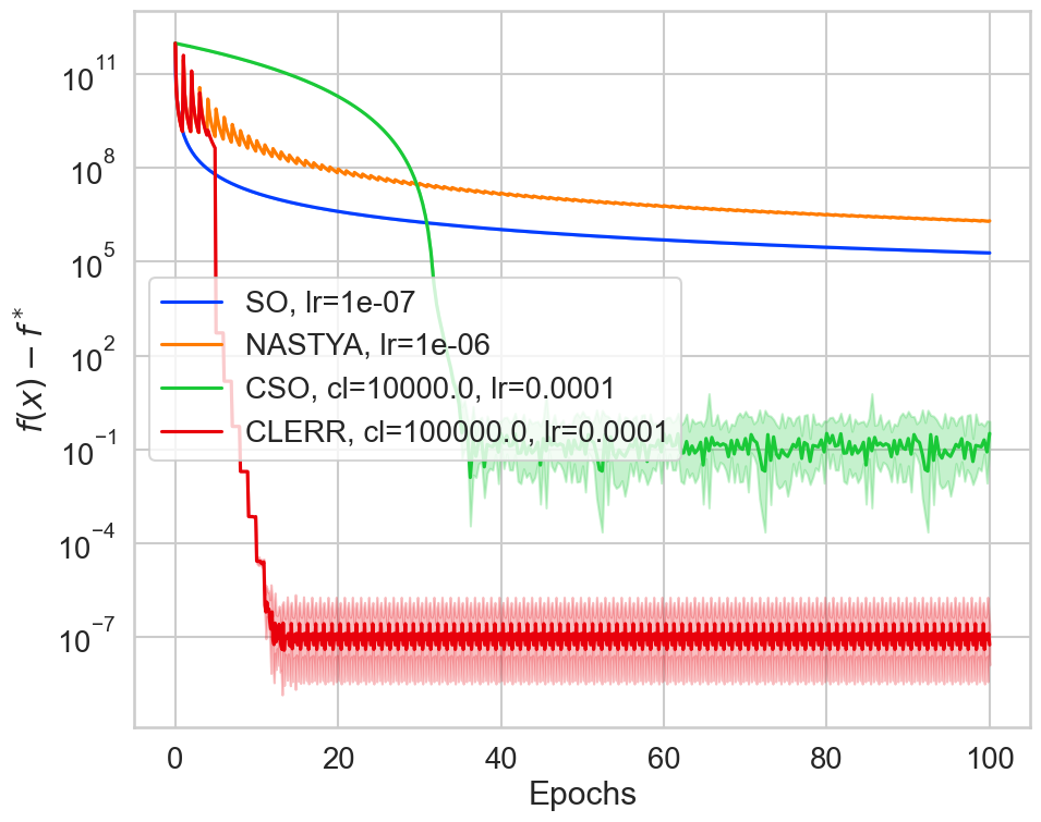
Figure 5: Function residual for (4), $\alpha_{t}=10^{-7}$. The best parameters are provided in the legend.

In these experiments we compare methods with random reshuffling, that shuffle data once at the start of training process. The main idea is to show the positive impact of random reshuffling and clipping on algorithm performance. We incorporate these two techniques inside our CLERR method (Algorithm 2).

Firstly, consider (4). For these experiments we take $d=1$ and randomly sample 1000 shifts $x_{i}\in[-10,10]$. We run all the methods for 10 different seeds on a logarithmic hyperparameter grid. Then we choose the best hyperparameters according to the best mean loss values on the second half of epochs. The parameter grid is provided in Table 1. To find $f^{*}$, we run the Newton method for couple iterations until convergence.

Since both Nastya and Algorithm 2 have jumping at the end of every epoch, if we tuned the inner stepsize along with other parameters, the inner stepsize would go to zero and the outer stepsize would be selected such as these methods solve the problem in 1 step. This would be unfair because other baselines do not use a jumping technique, so they would not be able to achieve such performance. Thus, we decided to fix the inner stepsize for Algorithm 2 and Nastya equal to the best stepsize, chosen for SO, and tune the clipping level and outer stepsize with the outer stepsize not exceeding the values supported in theory. Here and later, for simplicity, we speak about Algorithm 2 in terms of stepsize and clipping level, that we can obtain from $c_{0}$ and $c_{1}$ from (3). The best stepsize for SO is $10^{-7}$, so we choose inner stepsize for Nastya and Algorithm 2 the same. Nastya chooses outer stepsize equal $10^{-7}$, while CSO and CLERR (Algorithm 2) choose it equal to $10^{-4}$. CSO clips gradients at the level $10^{4}$, while CLERR – at the level $10^{5}$.

Method	Stepsize	Clipping Level	Inner Stepsize
SO	$[10^{-8},10^{-2}]$	-	-
NASTYA	$[10^{-8},10^{-2}]$	-	$10^{-7}$
CSO	$[10^{-8},10^{-2}]$	$[10^{0},10^{5}]$	-
Algorithm 2	$[10^{-8},10^{-2}]$	$[10^{0},10^{5}]$	$10^{-7}$

Table 1: Parameter grids for experiments on methods with random reshuffling on (4).

F.1.1 ResNet-18 on CIFAR-10

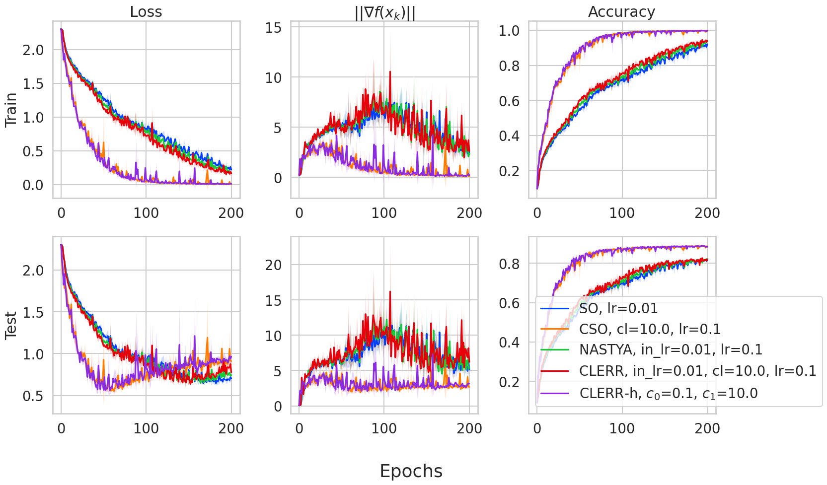
Figure 6: Loss, gradient norm and accuracy on train and test dataset for ResNet-18 on CIFAR-10. The best parameters are provided in the legend.

In this experiment we consider image classification task. We train ResNet-18 He et al. (2016) on the CIFAR-10 Krizhevsky et al. (2009) dataset. The implementation of ResNet-18 was taken from https://github.com/kuangliu/pytorch-cifar. All the methods are run on 3 different random seeds on logarithmic hyperparameter grid. Then we choose the best hyperparameters according to the best mean test accuracy on the last 25% of epochs.

In this experiment, we do not fix the inner stepsize for Nastya and CLERR, since methods do not try to make it as small as possible, as it was in the previous experiment. However, both SO, Nastya, and CLERR choose the same inner stepsize $10^{-2}$ as the best. Then, both Nastya and CLERR choose bigger outer step size $10^{-1}$, and CLERR also chooses clipping level on outer step size as $10$. Despite the fact that both Nastya and CLERR choose bigger outer stepsizes compared to inner stepsize, jumping does not have any impact on this problem. CLERR clips outer gradients at the level of $10$, so this also does not help method to converge to a better area.

Moreover, we provide results of heuristically modified Algorithm 2, where we fix clipping level and inner stepsize of Algorithm 2 equal to the best clipping level and the best stepsize from CSO correspondingly. The tunable parameters are only $c_{0}$ and $c_{1}$ for outer stepsize. We call this method CLERR-h. CLERR-h chooses an outer stepsize equal to $5$, while the clipping level is very tiny and equal to $10^{-2}$. All the parameter grids are provided in Table 2.

Method	Stepsize	Clipping Level	Inner Stepsize	$c_{0}$	$c_{1}$
RR	$[10^{-3},10^{-1}]$	-	-	-	-
NASTYA	$[10^{-3},10^{-1}]$	-	$[10^{-4},10^{0}]$	-	-
CRR	$[10^{-3},10^{-1}]$	$[10^{0},10^{3}]$	-	-	-
CLERR	$[10^{-3},10^{-1}]$	$[10^{0},10^{3}]$	$[10^{-4},10^{0}]$	-	-
CLERR-h	-	$10^{1}$	$10^{-1}$	$[10^{-2},10^{1}]$	$[10^{-2},10^{1}]$

Table 2: Parameter grids for experiments on methods with random reshuffling on ResNet-18 on CIFAR-10.

F.2 Methods with local steps

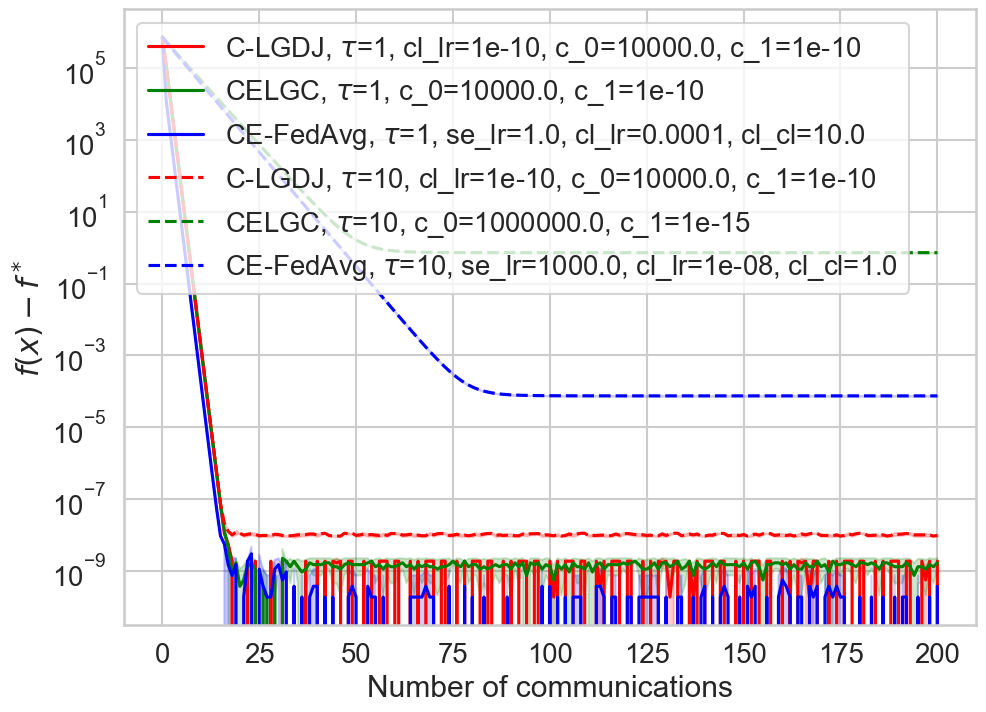
(a) $x_{0}=(1,...,1)$

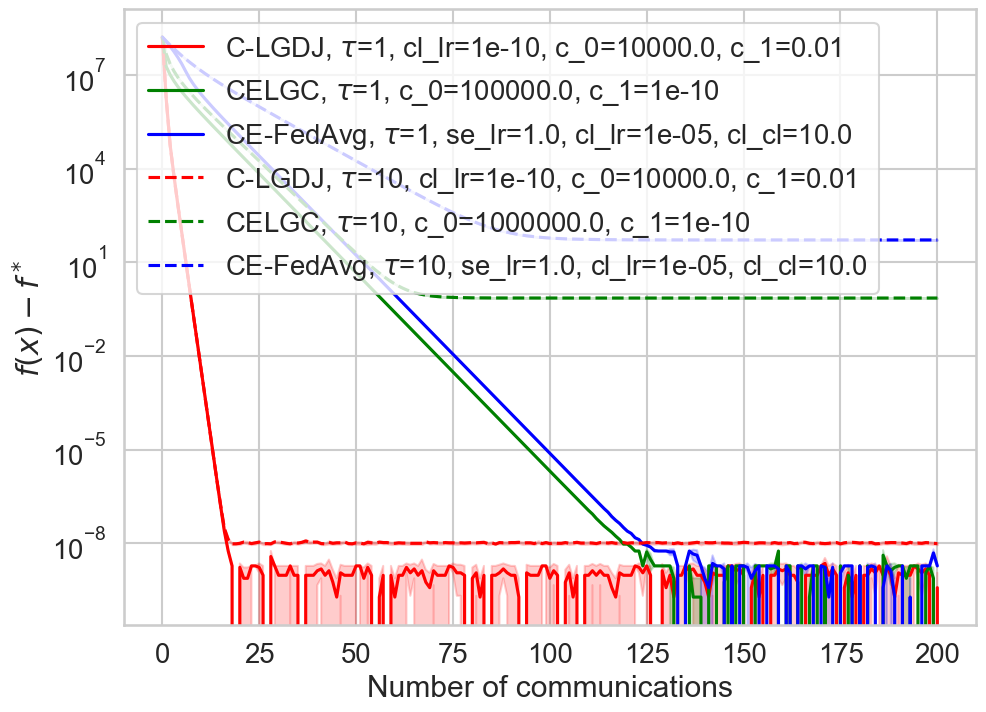
(b) $x_{0}=(10,...,10)$

Figure 7: Function residual for (4), starting from different $x_{0}$ for different number of local steps on the client device $\tau$. The best parameters are provided in the legend.

In these experiments we compare methods with local steps: Algorithm 1 (C-LGDJ) with Communication Efficient Local Gradient Clipping (CELGC) (Liu et al., 2022) and Clipping-Enabled-FedAvg (CE-FedAvg) Zhang et al. (2022). For comparison we take problem (4) for $d=100$, where we randomly sample 1000 shifts $x_{i}\in[-10,10]^{d}$. To make the distributions of data on each client more distinct between each other, we sort the whole dataset at the beginning of the experiment by $\|x_{i}\|$. Each method has 10 clients, where each client has equal number of data. We provide results for two starting points: $x_{0}=(1,...,1)$ and $x_{0}=(10,...,10)$. All the methods are run for 10 different random seeds on logarithmic hyperparameter grid. The best hyperparameters are chosen according to the best mean loss on the last 25% of epochs.

Each client performs $\tau=1$ or $\tau=10$ local steps, and each local step is performed on the whole local data. For ease of implementation and due to computational limitations we iterate over all the clients sequentially.

We reformulate constants $c_{0}$ and $c_{1}$ as server stepsize and clipping level from (3) to better interpret the experimental results. We start by paying attention to results with a single local step. Firstly, consider C-LGDJ (Algorithm 1). It chooses tiny client stepsizes $10^{-10}$ and small server stepsizes $5\cdot 10^{-5}$ for both starting points. For Figure 7(a) it also takes very big clipping level for server $10^{14}$, compared to Figure 7(b), where it clips on level $10^{6}$, which is obvious because on the second picture methods start farther from the minimum and have bigger gradients. Secondly, consider CELGC. In both cases, it takes very small client stepsizes: $5\cdot 10^{-5}$ and $5\cdot 10^{-6}$ respectively, and very big clipping levels: $10^{14}$ and $10^{15}$ respectively. Finally, CE-FedAvg also takes small client stepsizes: $10^{-4}$ and $10^{-5}$, rather big server stepsizes, which are equal to $1$, and average client clipping levels: $10$ in both cases. For $\tau=10$ we have the same parameters for C-LGDJ, CELGC tries to make even smaller steps with high clipping levels, while CE-FedAvg uses a much bigger server stepsize and much smaller client stepsize, for the case from Figure 7(a).

The grids of hyperparameters for $x_{0}=(1,...,1)$ are provided in Table 3, and for $x_{0}=(10,...,10)$ – in Table 4.

Method	Cl. Stepsize	Se. Stepsize	Cl. Clip Level	$c_{0}$	$c_{1}$
Clipped-L-SGD-J	$[10^{-10},10^{0}]$	-	-	$[10^{-10},10^{6}]$	$[10^{-10},10^{6}]$
CELGC	-	-	-	$[10^{-15},10^{10}]$	$[10^{-15},10^{10}]$
CE-FedAvg	$[10^{-10},10^{0}]$	$[10^{-10},10^{3}]$	$[10^{0},10^{4}]$	-	-

Table 3: Parameter grids for experiments on methods with local steps on (4) for $x_{0}=(1,...,1)$. Here "cl." means "Client", and "se." – "server".

Method	Cl. Stepsize	Se. Stepsize	Cl. Clip Level	$c_{0}$	$c_{1}$
Clipped-L-SGD-J	$[10^{-10},10^{0}]$	-	-	$[10^{-10},10^{6}]$	$[10^{-10},10^{6}]$
CELGC	-	-	-	$[10^{-10},10^{10}]$	$[10^{-10},10^{10}]$
CE-FedAvg	$[10^{-10},10^{0}]$	$[10^{-10},10^{0}]$	$[10^{0},10^{4}]$	-	-

Table 4: Parameter grids for experiments on methods with local steps on (4) for $x_{0}=(10,...,10)$. Here "cl." means "client", and "se." – "server".

F.3 Methods with local steps, random reshuffling and partial participation

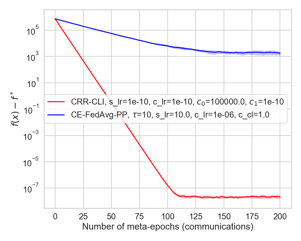
Figure 8: Function residual for (4), starting from $x_{0}=(1,...,1)$ with batch size 16. The best parameters are provided in the legend.

In these experiments we compare methods with clipping, random reshuffling, local steps and partial participation: Algorithm 3 (CRR-CLI) and with CE-FedAvg Zhang et al. (2022) with partial participation (CE-FedAvg-PP). For comparison we take problem (4) for $d=100$, where we randomly sample 1000 shifts $x_{i}\in[-10,10]^{d}$. Again, to make the distributions of data on each client more distinct between each other, we sort the whole dataset at the beginning of the experiment by $\|x_{i}\|$. All the methods are run for 10 different random seeds on logarithmic hyperparameter grid. The best hyperparameters are chosen according to the best mean loss on the last 25% of epochs.

Each method has 10 clients, where each client has the same amount of data. The size of the cohort is chosen to be 2. The method performs local steps on each client from the cohort, after which it performs communication and goes to the next cohort. In the Algorithm 3 the clients to the cohort are chosen sequentially with sliding window after Client-Reshuffling. In CE-FedAvg-PP clients to the cohort are always chosen randomly. The starting point is chosen $x_{0}=(1,...,1)$. All the methods are run for 10 different random seeds. The best hyperparameters are chosen according to the best mean loss on the last 25% of epochs.

For local steps we chose batch size equal to 16. In Algorithm 3 every client goes sequentially over the whole shuffled local dataset with batch size window. In CE-FedAvg-PP we fix number of local steps to 10, and each client samples batch on every local step.

Just like in previous experiment in Section 5.2, all the methods try to reduce the influence of local steps by making inner stepsizes very small. Algorithm 3 chooses both client and server stepsizes equal $10^{-10}$, and CE-FedAvg-PP chooses client stepsize equal $10^{-6}$ and client clipping level equals $1$. Speaking of outer steps, Algorithm 3 chooses global stepsize equal to $5\cdot 10^{-7}$ with clipping level $10^{16}$. And CE-FedAvg-PP has server stepsize equal to $10$. The grids of hyperparameters are provided in Table 5.

Method	Cl. Stepsize	Se. Stepsize	Cl. Clip Level	$c_{0}$	$c_{1}$
CRR-CLI	$[10^{-10},10^{6}]$	$[10^{-10},10^{6}]$	-	$[10^{-10},10^{5}]$	$[10^{-10},10^{5}]$
CE-FedAvg-PP	$[10^{-10},10^{3}]$	$[10^{-10},10^{3}]$	$[10^{0},10^{4}]$	-	-

Table 5: Parameter grids for experiments on methods with clipping, random reshuffling, local steps and partial participation. Here "cl." means "client", and "se." – "server".

Appendix G Additional experiments

In this section, we provide additional numerical experiments, that did not fit in the main paper: in Section G.1 we investigate the influence of that inner step size on the behavior of Algorithm 2, and in Section G.2 we provide additional experiments on logistic regression, where we compare Algorithm 2 with clipped SGD.

G.1 How the inner step size affects convergence of the method

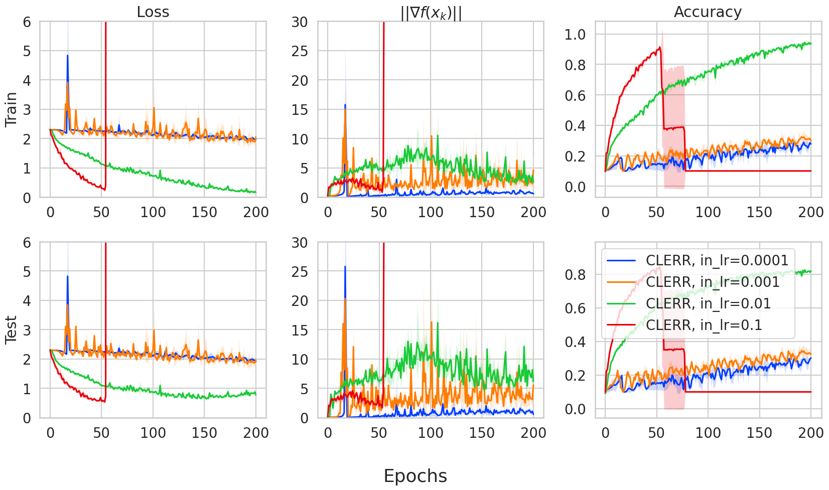
Figure 9: Algorithm 2 with different step sizes on ResNet-18 on CIFAR-10.

In this experiment, we investigate the influence of the inner step size on the behavior of Algorithm 2 on ResNet-18 on CIFAR-10. To do this, we take the same hyperparameters for Algorithm 2 as in Sections 5.1.1, F.1.1 and only change the inner step size. The results are provided in Figure 9.

On the one hand, if we take the inner step size too small (blue and orange lines), it converges very slowly. This is obvious since Algorithm 2 becomes regular Clipped-GD, which can be seen from pseudocode. Because Clipped-GD performs a single step per epoch, it has slow convergence. On the other hand, if we take the inner step size too big (red line), the method diverges. It does not have clipping on the inner step, so such behavior is expected. To summarize, it is important to take the inner step size small, but not too small, because it may slow down the convergence.

G.2 Logistic regression experiments

Since in the experiments on neural networks (Sections 5.1.1, F.1.1) regular CSO (SGD with clipping) showed very good results, we decided to conduct additional experiments on logistic regression, where we compare CSO with our Algorithm 2. We consider gisette and realsim datasets from libsvm library Chang & Lin (2011). All the methods are run for 3 different random seeds on logarithmic hyperparameter grid. The best hyperparameters are chosen according to the best mean loss on the last 25% of epochs. The results are presented in Figure 9.

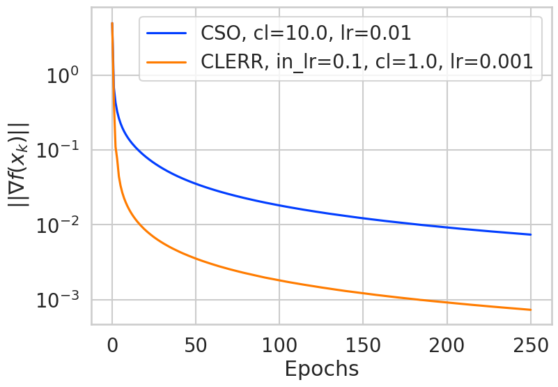
(a) gisette

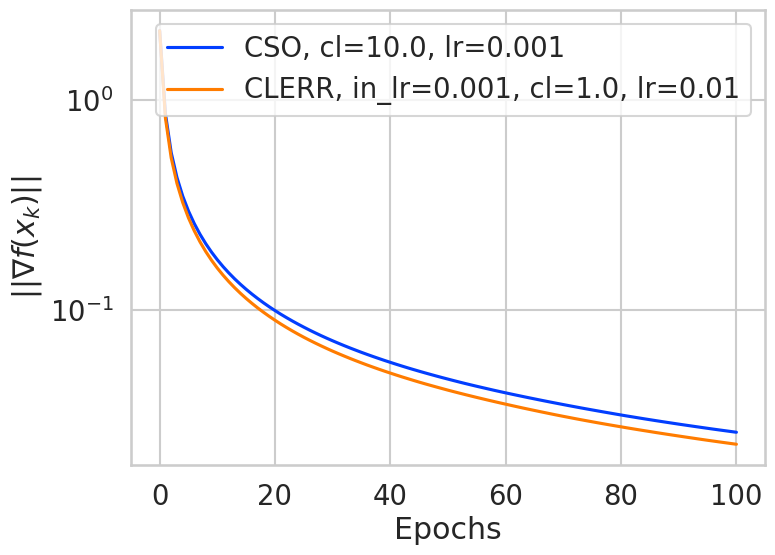
(b) realsim

Figure 10: Gradient norm for logistic regression problem on gisette and realsim datasets. The best parameters are provided in the legend.

Since the inner stepsize for CLERR has the same meaning as stepsize for CSO, we decided to take the same parameter grids for these two parameters. The same goes for clipping levels in spite of the fact that CLERR clips the gradient approximation only in the end of the epoch. This experiment shows that CLERR either has the same performance as CSO or better. Since logistic regression is ($L_{0},L_{1}$)-smooth, such result is expected, as Algorithm 2 is designed for such type of functions. Figure 10(a) shows us that CLERR chooses very small outer stepsize $10^{-3}$, while inner step size is bigger than the one in CSO: $10^{-1}$ vs $10^{-2}$. In the Figure 10(b) CLERR chooses parameters in the opposite way: inner step size is very small and equal to the one from CSO, while the outer stepsize is bigger. The parameter grids for gisette dataset is presented in Table 6, and for realsim – in Table 7.

	Stepsize	Clipping Level	Inner Stepsize
CSO	$[10^{-3},10^{-1}]$	$[10^{0},10^{2}]$	-
CLERR	$[10^{-3},10^{-1}]$	$[10^{0},10^{2}]$	$[10^{-3},10^{-1}]$

Table 6: Parameter grids for logistic regression experiments on gisette dataset

	Stepsize	Clipping Level	Inner Stepsize
CSO	$[10^{-5},10^{-1}]$	$[10^{0},10^{2}]$	-
CLERR	$[10^{-3},10^{-1}]$	$[10^{0},10^{2}]$	$[10^{-5},10^{-1}]$

Table 7: Parameter grids for logistic regression experiments on realsim dataset

Appendix H Extended Related Work

The usage of distributed methods is dictated by the fact that data can be naturally distributed across multiple devices/clients and be private, which is a typical scenario in Federated Learning (FL) (Konecný et al., 2016; McMahan et al., 2016; Kairouz et al., 2019). FL systems have practical considerations and are backed by extensive experiments from recent years. These highlight important effective design rules and algorithmic features. Below is a quick overview of some key points.

Partial Participation.

Partial Participation (PP) is a FL technique in which a server selects a subset of clients to engage in the training process during each communication round. Its application may be necessary in scenarios where server capacity or client availability is limited (Kairouz et al., 2021). The technique is useful when the number of clients is large, as the benefits of convergence do not grow proportionally with the size of the cohort (Charles et al., 2021). Clients can be selectively chosen to form a cohort, prioritizing those that deliver the most impactful information (Chen et al., 2020).

Local training.

Local Training (LT), where clients perform multiple optimization steps on their local data before engaging in the resource-intensive process of parameter synchronization, stands out as one of the most effective and practical techniques for training FL models. LT was proposed by Mangasarian (1995); Povey et al. (2014); Moritz et al. (2015) and later promoted by McMahan et al. (2016). While these works provided strong empirical evidence for the efficiency and potential of LT-based methods, they lacked theoretical backing. Early theoretical analyses of LT methods relied on restrictive data homogeneity assumptions, which are often unrealistic in real-world federated learning (FL) settings (Stich, 2018; Li et al., 2019; Haddadpour & Mahdavi, 2019). Later, Khaled et al. (2019a, b) removed limiting data homogeneity assumptions for LocalGD (Gradient Descent (GD) with LT). Then, Woodworth et al. (2020); Glasgow et al. (2022) derived lower bounds for GD with LT and data sampling, showing that its communication complexity is no better than minibatch Stochastic Gradient Descent (SGD) in settings with heterogeneous data. Another line of works focused on the mitigating so-called client drift phenomenon, which naturally occurs in LocalGD applied to distributed problems with heterogeneous local functions (Karimireddy et al., 2020; Tran-Dinh et al., 2021; Gorbunov et al., 2021b; Thapa et al., 2022; Mishchenko et al., 2022; Malinovsky et al., 2023b; Yi et al., 2024).

Although removing the dependence on data homogeneity was a key advancement, the theoretical result suggests LT worsens GD, which contradicts empirical evidence showing LT significantly improves it. Karimireddy et al. (2020) identified the client drift phenomenon as the main cause of the gap and proposed a solution to mitigate it, which led to the development of the Scaffold method, featuring the same communication complexity as GD. Later, another algorithm S-Local-GD was proposed by Gorbunov et al. (2021b). Finally, Mishchenko et al. (2022) demonstrated that a novel and simplified form of LT exemplified by their ProxSkip method, results in provable communication acceleration compared to GD. LocalGD is at the base of Federated Averaging (FedAvg) (McMahan et al., 2016). Essentially, FedAvg is a variant of LocalGD with participating devices and data sampled randomly. FedAvg has found applications in various ML tasks, such as, e.g., mobile keyboard prediction (Hard et al., 2018). Wide applicability of FedAvg motivates theoretical study of its backbone LocalGD algorithm.

Random reshuffling.

Stochastic Gradient Descent (SGD) serves as the foundation for nearly all advanced methods used to train supervised machine learning models. SGD is often refined with techniques like minibatching, momentum, and adaptive stepsizes. However, beyond these enhancements, it is important to decide how to select the next data point for training. Typically, variants of SGD apply a sampling with replacement approach where each new training data point is selected from the full dataset independently of previous samples. Although standard Stochastic Gradient Descent (SGD) (Robbins & Monro, 1951) is well-understood from a theoretical perspective (Rakhlin et al., 2012; Bottou et al., 2018; Nguyen et al., 2018; Gower et al., 2019; Drori & Shamir, 2020; Khaled & Richtárik, 2020; Sokolov, 2022; Demidovich et al., 2024), most widely-used ML frameworks rely on sampling without replacement, as it works better in the training neural networks (Bottou, 2009; Recht & Ré, 2013; Bengio, 2012; Sun, 2020). It leverages the finite-sum structure by ensuring each function is used once per epoch. However, this introduces bias: individual steps may not reflect full gradient descent steps on average. Thus, proving convergence requires more advanced techniques. Three popular variants of sampling without replacement are commonly used. Random Reshuffling (RR), where the training data is randomly reshuffled before the start of every epoch, is an extremely popular and well-studied approach. The aim of RR is to disrupt any potentially untoward default data sequencing that could hinder training efficiency. RR works very well in practice. Shuffle Once (SO) is analogous to RR, however, the training data is permuted randomly only once prior to the training process. The empirical performance is similar to RR. Incremental Gradient (IG) is identical to SO with the difference that the initial permutation is deterministic. This approach is the simplest, however, ineffective. IG has been extensively studied over a long period (Luo, 1991; Grippo, 1994; Li et al., 2022; Ying et al., 2019; Gürbüzbalaban et al., 2019; Nguyen et al., 2021). A major challenge with IG lies in selecting a particular permutation for cycling through the iterations, a task that Nedic & Bertsekas (2001) highlight as being quite difficult. (Bertsekas, 2015) provides an example that underscores the vulnerability of IG to poor orderings, especially when contrasted with RR. Meaningful theoretical analyses of the SO method have only emerged recently (Safran & Shamir, 2020; Rajput et al., 2020). RR has been shown to outperform both SGD and IG for objectives that are twice-smooth (Gürbüzbalaban et al., 2015; Haochen & Sra, 2019). Jain et al. (2019) examine the convergence of RR for smooth objectives. Safran & Shamir (2020); Rajput et al. (2020) provide lower bounds for RR. Mishchenko et al. (2020) recently conducted a thorough analysis of IG, SO and RR using innovative and simplified proof techniques, resulting in better convergence rates. Recent advances on RR can be found in (Sadiev et al., 2022; Cha et al., 2023; Cai et al., 2023; Koloskova et al., 2023b).

Other useful features.

Further techniques in FL include compression during the communication rounds (Alistarh et al., 2018; Gorbunov et al., 2021a; Panferov et al., 2024), clients’ drift reduction (Karimireddy et al., 2020; Gorbunov et al., 2021b).

References

• Ahn et al. (2023) Kwangjun Ahn, Xiang Cheng, Minhak Song, Chulhee Yun, Ali Jadbabaie, and Suvrit Sra. Linear attention is (maybe) all you need (to understand transformer optimization). ArXiv, abs/2310.01082, 2023. URL https://api.semanticscholar.org/CorpusID:263605847.
• Alistarh et al. (2018) Dan Alistarh, Torsten Hoefler, Mikael Johansson, Sarit Khirirat, Nikola Konstantinov, and Cédric Renggli. The convergence of sparsified gradient methods. In Proceedings of the 32nd International Conference on Neural Information Processing Systems, NIPS’18, pp.  5977–5987, Red Hook, NY, USA, 2018. Curran Associates Inc.
• Bengio (2012) Yoshua Bengio. Practical recommendations for gradient-based training of deep architectures. In Neural Networks, 2012. URL https://api.semanticscholar.org/CorpusID:10808461.
• Bertsekas (2015) Dimitri P. Bertsekas. Incremental gradient, subgradient, and proximal methods for convex optimization: A survey. ArXiv, abs/1507.01030, 2015.
• Bottou (2009) Léon Bottou. Curiously fast convergence of some stochastic gradient descent algorithms. 2009. URL https://api.semanticscholar.org/CorpusID:16822133.
• Bottou et al. (2018) Léon Bottou, Frank E. Curtis, and Jorge Nocedal. Optimization methods for large-scale machine learning. SIAM Review, 60(2):223–311, 2018. doi:10.1137/16M1080173. URL https://doi.org/10.1137/16M1080173.
• Brown et al. (2020) Tom Brown, Benjamin Mann, Nick Ryder, Melanie Subbiah, Jared D Kaplan, Prafulla Dhariwal, Arvind Neelakantan, Pranav Shyam, Girish Sastry, Amanda Askell, Sandhini Agarwal, Ariel Herbert-Voss, Gretchen Krueger, Tom Henighan, Rewon Child, Aditya Ramesh, Daniel Ziegler, Jeffrey Wu, Clemens Winter, Chris Hesse, Mark Chen, Eric Sigler, Mateusz Litwin, Scott Gray, Benjamin Chess, Jack Clark, Christopher Berner, Sam McCandlish, Alec Radford, Ilya Sutskever, and Dario Amodei. Language models are few-shot learners. In H. Larochelle, M. Ranzato, R. Hadsell, M.F. Balcan, and H. Lin (eds.), Advances in Neural Information Processing Systems, volume 33, pp.  1877–1901. Curran Associates, Inc., 2020. URL https://proceedings.neurips.cc/paper_files/paper/2020/file/1457c0d6bfcb4967418bfb8ac142f64a-Paper.pdf.
• Cai et al. (2023) Xufeng Cai, Cheuk Yin Lin, and Jelena Diakonikolas. Empirical risk minimization with shuffled SGD: A primal-dual perspective and improved bounds. CoRR, abs/2306.12498, 2023. doi:10.48550/ARXIV.2306.12498. URL https://doi.org/10.48550/arXiv.2306.12498.
• Cha et al. (2023) Jaeyoung Cha, Jaewook Lee, and Chulhee Yun. Tighter lower bounds for shuffling sgd: random permutations and beyond. In Proceedings of the 40th International Conference on Machine Learning, ICML’23. JMLR.org, 2023.
• Chang & Lin (2011) Chih-Chung Chang and Chih-Jen Lin. LIBSVM: A library for support vector machines. ACM Transactions on Intelligent Systems and Technology, 2:27:1–27:27, 2011. Software available at http://www.csie.ntu.edu.tw/˜cjlin/libsvm.
• Charles et al. (2021) Zachary Charles, Zachary Garrett, Zhouyuan Huo, Sergei Shmulyian, and Virginia Smith. On large-cohort training for federated learning. In M. Ranzato, A. Beygelzimer, Y. Dauphin, P.S. Liang, and J. Wortman Vaughan (eds.), Advances in Neural Information Processing Systems, volume 34, pp.  20461–20475. Curran Associates, Inc., 2021. URL https://proceedings.neurips.cc/paper_files/paper/2021/file/ab9ebd57177b5106ad7879f0896685d4-Paper.pdf.
• Chen et al. (2020) Wenlin Chen, Samuel Horváth, and Peter Richtárik. Optimal client sampling for federated learning. Trans. Mach. Learn. Res., 2022, 2020. URL https://api.semanticscholar.org/CorpusID:225068165.
• Chen et al. (2023) Ziyi Chen, Yi Zhou, Yingbin Liang, and Zhaosong Lu. Generalized-smooth nonconvex optimization is as efficient as smooth nonconvex optimization. In Proceedings of the 40th International Conference on Machine Learning, ICML’23. JMLR.org, 2023.
• Crawshaw et al. (2024) Michael Crawshaw, Mingrui Liu, Francesco Orabona, Wei Zhang, and Zhenxun Zhuang. Robustness to unbounded smoothness of generalized signsgd. In Proceedings of the 36th International Conference on Neural Information Processing Systems, NIPS ’22, Red Hook, NY, USA, 2024. Curran Associates Inc. ISBN 9781713871088.
• Defazio & Bottou (2019) Aaron Defazio and Léon Bottou. On the ineffectiveness of variance reduced optimization for deep learning. Advances in Neural Information Processing Systems, 32, 2019.
• Demidovich et al. (2024) Yury Demidovich, Grigory Malinovsky, Igor Sokolov, and Peter Richtárik. A guide through the zoo of biased sgd. In Proceedings of the 37th International Conference on Neural Information Processing Systems, NIPS ’23, Red Hook, NY, USA, 2024. Curran Associates Inc.
• Drori & Shamir (2020) Yoel Drori and Ohad Shamir. The complexity of finding stationary points with stochastic gradient descent. In Hal Daumé III and Aarti Singh (eds.), Proceedings of the 37th International Conference on Machine Learning, volume 119 of Proceedings of Machine Learning Research, pp.  2658–2667. PMLR, 13–18 Jul 2020. URL https://proceedings.mlr.press/v119/drori20a.html.
• Glasgow et al. (2022) Margalit R. Glasgow, Honglin Yuan, and Tengyu Ma. Sharp bounds for federated averaging (local sgd) and continuous perspective. In Gustau Camps-Valls, Francisco J. R. Ruiz, and Isabel Valera (eds.), Proceedings of The 25th International Conference on Artificial Intelligence and Statistics, volume 151 of Proceedings of Machine Learning Research, pp.  9050–9090. PMLR, 28–30 Mar 2022. URL https://proceedings.mlr.press/v151/glasgow22a.html.
• Gorbunov et al. (2021a) Eduard Gorbunov, Konstantin P. Burlachenko, Zhize Li, and Peter Richtarik. Marina: Faster non-convex distributed learning with compression. In Marina Meila and Tong Zhang (eds.), Proceedings of the 38th International Conference on Machine Learning, volume 139 of Proceedings of Machine Learning Research, pp.  3788–3798. PMLR, 18–24 Jul 2021a.
• Gorbunov et al. (2021b) Eduard Gorbunov, Filip Hanzely, and Peter Richtarik. Local sgd: Unified theory and new efficient methods. In Arindam Banerjee and Kenji Fukumizu (eds.), Proceedings of The 24th International Conference on Artificial Intelligence and Statistics, volume 130 of Proceedings of Machine Learning Research, pp. 3556–3564. PMLR, 13–15 Apr 2021b. URL https://proceedings.mlr.press/v130/gorbunov21a.html.
• Gorbunov et al. (2024) Eduard Gorbunov, Nazarii Tupitsa, Sayantan Choudhury, Alen Aliev, Peter Richtárik, Samuel Horváth, and Martin Takáč. Methods for convex $(l_{0},l_{1})$-smooth optimization: Clipping, acceleration, and adaptivity, 2024. URL https://arxiv.org/abs/2409.14989.
• Gower et al. (2019) Robert Mansel Gower, Nicolas Loizou, Xun Qian, Alibek Sailanbayev, Egor Shulgin, and Peter Richtárik. SGD: General analysis and improved rates. In Kamalika Chaudhuri and Ruslan Salakhutdinov (eds.), Proceedings of the 36th International Conference on Machine Learning, volume 97 of Proceedings of Machine Learning Research, pp. 5200–5209. PMLR, 09–15 Jun 2019. URL https://proceedings.mlr.press/v97/qian19b.html.
• Goyal et al. (2017) Priya Goyal, Piotr Dollár, Ross B. Girshick, Pieter Noordhuis, Lukasz Wesolowski, Aapo Kyrola, Andrew Tulloch, Yangqing Jia, and Kaiming He. Accurate, large minibatch sgd: Training imagenet in 1 hour. ArXiv, abs/1706.02677, 2017.
• Grippo (1994) Luigi Grippo. A class of unconstrained minimization methods for neural network training. Optimization Methods & Software, 4:135–150, 1994.
• Gürbüzbalaban et al. (2019) M. Gürbüzbalaban, A. Ozdaglar, and P. A. Parrilo. Convergence rate of incremental gradient and incremental newton methods. SIAM Journal on Optimization, 29(4):2542–2565, 2019. doi:10.1137/17M1147846. URL https://doi.org/10.1137/17M1147846.
• Gürbüzbalaban et al. (2015) Mert Gürbüzbalaban, Asuman E. Ozdaglar, and Pablo A. Parrilo. Why random reshuffling beats stochastic gradient descent. Mathematical Programming, 186:49 – 84, 2015.
• Haddadpour & Mahdavi (2019) Farzin Haddadpour and Mehrdad Mahdavi. On the convergence of local descent methods in federated learning. ArXiv, abs/1910.14425, 2019.
• Haochen & Sra (2019) Jeff Haochen and Suvrit Sra. Random shuffling beats SGD after finite epochs. In Kamalika Chaudhuri and Ruslan Salakhutdinov (eds.), Proceedings of the 36th International Conference on Machine Learning, volume 97 of Proceedings of Machine Learning Research, pp. 2624–2633. PMLR, 09–15 Jun 2019. URL https://proceedings.mlr.press/v97/haochen19a.html.
• Hard et al. (2018) Andrew Straiton Hard, Kanishka Rao, Rajiv Mathews, Françoise Beaufays, Sean Augenstein, Hubert Eichner, Chloé Kiddon, and Daniel Ramage. Federated learning for mobile keyboard prediction. ArXiv, abs/1811.03604, 2018. URL https://api.semanticscholar.org/CorpusID:53207681.
• He et al. (2016) Kaiming He, Xiangyu Zhang, Shaoqing Ren, and Jian Sun. Deep residual learning for image recognition. In Proceedings of the IEEE conference on computer vision and pattern recognition, pp.  770–778, 2016.
• Jain et al. (2019) Prateek Jain, Dheeraj M. Nagaraj, and Praneeth Netrapalli. Sgd without replacement: Sharper rates for general smooth convex functions. ArXiv, abs/1903.01463, 2019.
• Jin et al. (2021) Jikai Jin, Bohang Zhang, Haiyang Wang, and Liwei Wang. Non-convex distributionally robust optimization: Non-asymptotic analysis. Advances in Neural Information Processing Systems, 34:2771–2782, 2021.
• Kairouz et al. (2019) Peter Kairouz, H. B. McMahan, Brendan Avent, Aurélien Bellet, Mehdi Bennis, Arjun Nitin Bhagoji, Keith Bonawitz, Zachary B. Charles, Graham Cormode, Rachel Cummings, Rafael G. L. D’Oliveira, Salim Y. El Rouayheb, David Evans, Josh Gardner, Zachary Garrett, Adrià Gascón, Badih Ghazi, Phillip B. Gibbons, Marco Gruteser, Zaïd Harchaoui, Chaoyang He, Lie He, Zhouyuan Huo, Ben Hutchinson, Justin Hsu, Martin Jaggi, Tara Javidi, Gauri Joshi, Mikhail Khodak, Jakub Konecný, Aleksandra Korolova, Farinaz Koushanfar, Oluwasanmi Koyejo, Tancrède Lepoint, Yang Liu, Prateek Mittal, Mehryar Mohri, Richard Nock, Ayfer Özgür, R. Pagh, Mariana Raykova, Hang Qi, Daniel Ramage, Ramesh Raskar, Dawn Xiaodong Song, Weikang Song, Sebastian U. Stich, Ziteng Sun, Ananda Theertha Suresh, Florian Tramèr, Praneeth Vepakomma, Jianyu Wang, Li Xiong, Zheng Xu, Qiang Yang, Felix X. Yu, Han Yu, and Sen Zhao. Advances and open problems in federated learning. Found. Trends Mach. Learn., 14:1–210, 2019.
• Kairouz et al. (2021) Peter Kairouz, H. Brendan McMahan, Brendan Avent, Aurélien Bellet, Mehdi Bennis, Arjun Nitin Bhagoji, Kallista Bonawitz, Zachary Charles, Graham Cormode, Rachel Cummings, Rafael G. L. D’Oliveira, Hubert Eichner, Salim El Rouayheb, David Evans, Josh Gardner, Zachary Garrett, Adrià Gascón, Badih Ghazi, Phillip B. Gibbons, Marco Gruteser, Zaid Harchaoui, Chaoyang He, Lie He, Zhouyuan Huo, Ben Hutchinson, Justin Hsu, Martin Jaggi, Tara Javidi, Gauri Joshi, Mikhail Khodak, Jakub Konecný, Aleksandra Korolova, Farinaz Koushanfar, Sanmi Koyejo, Tancrède Lepoint, Yang Liu, Prateek Mittal, Mehryar Mohri, Richard Nock, Ayfer Özgür, Rasmus Pagh, Hang Qi, Daniel Ramage, Ramesh Raskar, Mariana Raykova, Dawn Song, Weikang Song, Sebastian U. Stich, Ziteng Sun, Ananda Theertha Suresh, Florian Tramèr, Praneeth Vepakomma, Jianyu Wang, Li Xiong, Zheng Xu, Qiang Yang, Felix X. Yu, Han Yu, and Sen Zhao. Advances and open problems in federated learning. Found. Trends Mach. Learn., 14(1–2):1–210, June 2021. ISSN 1935-8237. doi:10.1561/2200000083. URL https://doi.org/10.1561/2200000083.
• Karimireddy et al. (2020) Sai Praneeth Karimireddy, Satyen Kale, Mehryar Mohri, Sashank Reddi, Sebastian Stich, and Ananda Theertha Suresh. SCAFFOLD: Stochastic controlled averaging for federated learning. In Hal Daumé III and Aarti Singh (eds.), Proceedings of the 37th International Conference on Machine Learning, volume 119 of Proceedings of Machine Learning Research, pp.  5132–5143. PMLR, 13–18 Jul 2020. URL https://proceedings.mlr.press/v119/karimireddy20a.html.
• Khaled & Richtárik (2020) Ahmed Khaled and Peter Richtárik. Better theory for sgd in the nonconvex world. ArXiv, abs/2002.03329, 2020. URL https://api.semanticscholar.org/CorpusID:211069380.
• Khaled et al. (2019a) Ahmed Khaled, Konstantin Mishchenko, and Peter Richtárik. First analysis of local gd on heterogeneous data. ArXiv, abs/1909.04715, 2019a.
• Khaled et al. (2019b) Ahmed Khaled, Konstantin Mishchenko, and Peter Richtárik. Tighter theory for local sgd on identical and heterogeneous data. In International Conference on Artificial Intelligence and Statistics, 2019b.
• Kolesnikov et al. (2019) Alexander Kolesnikov, Lucas Beyer, Xiaohua Zhai, Joan Puigcerver, Jessica Yung, Sylvain Gelly, and Neil Houlsby. Big transfer (bit): General visual representation learning. In European Conference on Computer Vision, 2019.
• Koloskova et al. (2020) Anastasia Koloskova, Nicolas Loizou, Sadra Boreiri, Martin Jaggi, and Sebastian U. Stich. A unified theory of decentralized sgd with changing topology and local updates. In Proceedings of the 37th International Conference on Machine Learning, ICML’20. JMLR.org, 2020.
• Koloskova et al. (2023a) Anastasia Koloskova, Hadrien Hendrikx, and Sebastian U. Stich. Revisiting gradient clipping: stochastic bias and tight convergence guarantees. In Proceedings of the 40th International Conference on Machine Learning, ICML’23. JMLR.org, 2023a.
• Koloskova et al. (2023b) Anastasia Koloskova, Ryan McKenna, Zachary B. Charles, Keith Rush, and Brendan McMahan. Convergence of gradient descent with linearly correlated noise and applications to differentially private learning. ArXiv, abs/2302.01463, 2023b. URL https://api.semanticscholar.org/CorpusID:256598052.
• Konecný et al. (2016) Jakub Konecný, H. B. McMahan, Felix X. Yu, Peter Richtárik, Ananda Theertha Suresh, and Dave Bacon. Federated learning: Strategies for improving communication efficiency. ArXiv, abs/1610.05492, 2016.
• Krizhevsky et al. (2009) Alex Krizhevsky, Geoffrey Hinton, et al. Learning multiple layers of features from tiny images. 2009.
• Le Scao et al. (2023) Teven Le Scao, Angela Fan, Christopher Akiki, Ellie Pavlick, Suzana Ilić, Daniel Hesslow, Roman Castagné, Alexandra Sasha Luccioni, François Yvon, Matthias Gallé, et al. Bloom: A 176b-parameter open-access multilingual language model. 2023.
• Li (2020) Chuan Li. Demystifying gpt-3 language model: A technical overview, 2020. URL https://lambdalabs.com/blog/demystifying-gpt-3.
• Li et al. (2024a) Haochuan Li, Jian Qian, Yi Tian, Alexander Rakhlin, and Ali Jadbabaie. Convex and non-convex optimization under generalized smoothness. NIPS ’23, Red Hook, NY, USA, 2024a. Curran Associates Inc.
• Li et al. (2024b) Haochuan Li, Alexander Rakhlin, and Ali Jadbabaie. Convergence of adam under relaxed assumptions. In Proceedings of the 37th International Conference on Neural Information Processing Systems, NIPS ’23, Red Hook, NY, USA, 2024b. Curran Associates Inc.
• Li et al. (2019) Xiang Li, Kaixuan Huang, Wenhao Yang, Shusen Wang, and Zhihua Zhang. On the convergence of fedavg on non-iid data. ArXiv, abs/1907.02189, 2019.
• Li et al. (2022) Xiao Li, Zhihui Zhu, Anthony Man-Cho So, and Jason D Lee. Incremental methods for weakly convex optimization, 2022. URL https://arxiv.org/abs/1907.11687.
• Liu et al. (2022) Mingrui Liu, Zhenxun Zhuang, Yunwen Lei, and Chunyang Liao. A communication-efficient distributed gradient clipping algorithm for training deep neural networks. Advances in Neural Information Processing Systems, 35:26204–26217, 2022.
• Lojasiewicz (1963) Stanislaw Lojasiewicz. A topological property of real analytic subsets. Coll. du CNRS, Les équations aux dérivées partielles, 117(87-89):2, 1963.
• Luo (1991) Zhi-Quan Tom Luo. On the convergence of the lms algorithm with adaptive learning rate for linear feedforward networks. Neural Computation, 3:226–245, 1991.
• Malinovsky et al. (2022) Grigory Malinovsky, Konstantin Mishchenko, and Peter Richtárik. Server-side stepsizes and sampling without replacement provably help in federated optimization. Proceedings of the 4th International Workshop on Distributed Machine Learning, 2022.
• Malinovsky et al. (2023a) Grigory Malinovsky, Samuel Horv’ath, Konstantin Burlachenko, and Peter Richt’arik. Federated learning with regularized client participation. ArXiv, abs/2302.03662, 2023a. URL https://api.semanticscholar.org/CorpusID:256627753.
• Malinovsky et al. (2023b) Grigory Malinovsky, Konstantin Mishchenko, and Peter Richtárik. Server-side stepsizes and sampling without replacement provably help in federated optimization. In Proceedings of the 4th International Workshop on Distributed Machine Learning, DistributedML ’23, pp.  85–104, New York, NY, USA, 2023b. Association for Computing Machinery. ISBN 9798400704475. doi:10.1145/3630048.3630187. URL https://doi.org/10.1145/3630048.3630187.
• Mangasarian (1995) LO Mangasarian. Parallel gradient distribution in unconstrained optimization. SIAM Journal on Control and Optimization, 1995.
• McMahan et al. (2016) H. B. McMahan, Eider Moore, Daniel Ramage, Seth Hampson, and Blaise Agüera y Arcas. Communication-efficient learning of deep networks from decentralized data. In International Conference on Artificial Intelligence and Statistics, 2016.
• Mishchenko et al. (2020) Konstantin Mishchenko, Ahmed Khaled, and Peter Richtárik. Random reshuffling: Simple analysis with vast improvements. In H. Larochelle, M. Ranzato, R. Hadsell, M.F. Balcan, and H. Lin (eds.), Advances in Neural Information Processing Systems, volume 33, pp.  17309–17320. Curran Associates, Inc., 2020. URL https://proceedings.neurips.cc/paper_files/paper/2020/file/c8cc6e90ccbff44c9cee23611711cdc4-Paper.pdf.
• Mishchenko et al. (2022) Konstantin Mishchenko, Grigory Malinovsky, Sebastian Stich, and Peter Richtarik. ProxSkip: Yes! Local gradient steps provably lead to communication acceleration! Finally! In Kamalika Chaudhuri, Stefanie Jegelka, Le Song, Csaba Szepesvari, Gang Niu, and Sivan Sabato (eds.), Proceedings of the 39th International Conference on Machine Learning, volume 162 of Proceedings of Machine Learning Research, pp.  15750–15769. PMLR, 17–23 Jul 2022. URL https://proceedings.mlr.press/v162/mishchenko22b.html.
• Moritz et al. (2015) Philipp Moritz, Robert Nishihara, Ion Stoica, and Michael I. Jordan. Sparknet: Training deep networks in spark. CoRR, abs/1511.06051, 2015.
• Nedic & Bertsekas (2001) Angelia Nedic and Dimitri P. Bertsekas. Incremental subgradient methods for nondifferentiable optimization. SIAM Journal on Optimization, 12(1):109–138, 2001. doi:10.1137/S1052623499362111. URL https://doi.org/10.1137/S1052623499362111.
• Nguyen et al. (2021) Lam M. Nguyen, Quoc Tran-Dinh, Dzung T. Phan, Phuong Ha Nguyen, and Marten Van Dijk. A unified convergence analysis for shuffling-type gradient methods. J. Mach. Learn. Res., 22(1), jan 2021. ISSN 1532-4435.
• Nguyen et al. (2018) Phuong Ha Nguyen, Lam M. Nguyen, and Marten van Dijk. Tight dimension independent lower bound on the expected convergence rate for diminishing step sizes in sgd. In Neural Information Processing Systems, 2018. URL https://api.semanticscholar.org/CorpusID:52965883.
• Panferov et al. (2024) Andrei Panferov, Yury Demidovich, Ahmad Rammal, and Peter Richtárik. Correlated quantization for faster nonconvex distributed optimization, 2024. URL https://arxiv.org/abs/2401.05518.
• Pascanu et al. (2013) Razvan Pascanu, Tomas Mikolov, and Yoshua Bengio. On the difficulty of training recurrent neural networks. In Proceedings of the 30th International Conference on International Conference on Machine Learning-Volume 28, 2013.
• Polyak (1963) Boris Polyak. Gradient methods for the minimisation of functionals. Ussr Computational Mathematics and Mathematical Physics, 3:864–878, 1963.
• Povey et al. (2014) Daniel Povey, Xiaohui Zhang, and Sanjeev Khudanpur. Parallel training of deep neural networks with natural gradient and parameter averaging. In International Conference on Learning Representations, 2014.
• Qian et al. (2021) Jiang Qian, Yuren Wu, Bojin Zhuang, Shaojun Wang, and Jing Xiao. Understanding gradient clipping in incremental gradient methods. In Arindam Banerjee and Kenji Fukumizu (eds.), Proceedings of The 24th International Conference on Artificial Intelligence and Statistics, volume 130 of Proceedings of Machine Learning Research, pp. 1504–1512. PMLR, 13–15 Apr 2021. URL https://proceedings.mlr.press/v130/qian21a.html.
• Rajput et al. (2020) Shashank Rajput, Anant Gupta, and Dimitris Papailiopoulos. Closing the convergence gap of SGD without replacement. In Hal Daumé III and Aarti Singh (eds.), Proceedings of the 37th International Conference on Machine Learning, volume 119 of Proceedings of Machine Learning Research, pp.  7964–7973. PMLR, 13–18 Jul 2020. URL https://proceedings.mlr.press/v119/rajput20a.html.
• Rakhlin et al. (2012) Alexander Rakhlin, Ohad Shamir, and Karthik Sridharan. Making gradient descent optimal for strongly convex stochastic optimization. In Proceedings of the 29th International Coference on International Conference on Machine Learning, ICML’12, pp.  1571–1578, Madison, WI, USA, 2012. Omnipress. ISBN 9781450312851.
• Recht & Ré (2013) Benjamin Recht and Christopher Ré. Parallel stochastic gradient algorithms for large-scale matrix completion. Mathematical Programming Computation, 5:201 – 226, 2013. URL https://api.semanticscholar.org/CorpusID:17109415.
• Robbins & Monro (1951) Herbert Robbins and Sutton Monro. A Stochastic Approximation Method. The Annals of Mathematical Statistics, 22(3):400 – 407, 1951. doi:10.1214/aoms/1177729586. URL https://doi.org/10.1214/aoms/1177729586.
• Sadiev et al. (2022) Abdurakhmon Sadiev, Grigory Malinovsky, Eduard Gorbunov, Igor Sokolov, Ahmed Khaled, Konstantin Burlachenko, and Peter Richtárik. Federated optimization algorithms with random reshuffling and gradient compression, 2022. URL https://arxiv.org/abs/2206.07021.
• Safran & Shamir (2020) Itay Safran and Ohad Shamir. How good is sgd with random shuffling? In Jacob Abernethy and Shivani Agarwal (eds.), Proceedings of Thirty Third Conference on Learning Theory, volume 125 of Proceedings of Machine Learning Research, pp.  3250–3284. PMLR, 09–12 Jul 2020. URL https://proceedings.mlr.press/v125/safran20a.html.
• Sokolov (2022) I. Sokolov. Non-convex stochastic optimization with biased gradient estimators, 2022.
• Stich (2018) Sebastian U Stich. Local sgd converges fast and communicates little. arXiv preprint arXiv:1805.09767, 2018.
• Sun (2020) Ruoyu Sun. Optimization for deep learning: An overview. Journal of the Operations Research Society of China, 8:249 – 294, 2020. URL https://api.semanticscholar.org/CorpusID:220511793.
• Thapa et al. (2022) Chandra Thapa, Mahawaga Arachchige Pathum Chamikara, Seyit Camtepe, and Lichao Sun. Splitfed: When federated learning meets split learning. In AAAI, pp.  8485–8493. AAAI Press, 2022. ISBN 978-1-57735-876-3.
• Tran-Dinh et al. (2021) Quoc Tran-Dinh, Nhan H. Pham, D. Phan, and Lam M. Nguyen. Feddr - randomized douglas-rachford splitting algorithms for nonconvex federated composite optimization. In Neural Information Processing Systems, 2021. URL https://api.semanticscholar.org/CorpusID:235376727.
• Wang et al. (2024) Bohan Wang, Yushun Zhang, Huishuai Zhang, Qi Meng, Ruoyu Sun, Zhi-Ming Ma, Tie-Yan Liu, Zhi-Quan Luo, and Wei Chen. Provable adaptivity of adam under non-uniform smoothness. In Proceedings of the 30th ACM SIGKDD Conference on Knowledge Discovery and Data Mining, KDD ’24, pp.  2960–2969, New York, NY, USA, 2024. Association for Computing Machinery. ISBN 9798400704901. doi:10.1145/3637528.3671718. URL https://doi.org/10.1145/3637528.3671718.
• Woodworth et al. (2020) Blake Woodworth, Kumar Kshitij Patel, and Nathan Srebro. Minibatch vs local sgd for heterogeneous distributed learning. In Proceedings of the 34th International Conference on Neural Information Processing Systems, NIPS ’20, Red Hook, NY, USA, 2020. Curran Associates Inc. ISBN 9781713829546.
• Yi et al. (2024) Kai Yi, Timur Kharisov, Igor Sokolov, and Peter Richtárik. Cohort squeeze: Beyond a single communication round per cohort in cross-device federated learning, 2024. URL https://arxiv.org/abs/2406.01115.
• Ying et al. (2019) Bicheng Ying, Kun Yuan, Stefan Vlaski, and Ali H. Sayed. Stochastic learning under random reshuffling with constant step-sizes. IEEE Transactions on Signal Processing, 67(2):474–489, 2019. doi:10.1109/TSP.2018.2878551.
• You et al. (2019) Yang You, Jing Li, Sashank J. Reddi, Jonathan Hseu, Sanjiv Kumar, Srinadh Bhojanapalli, Xiaodan Song, James Demmel, Kurt Keutzer, and Cho-Jui Hsieh. Large batch optimization for deep learning: Training bert in 76 minutes. arXiv: Learning, 2019.
• Zhang et al. (2020a) Bohang Zhang, Jikai Jin, Cong Fang, and Liwei Wang. Improved analysis of clipping algorithms for non-convex optimization. In Proceedings of the 34th International Conference on Neural Information Processing Systems, NIPS ’20, Red Hook, NY, USA, 2020a. Curran Associates Inc. ISBN 9781713829546.
• Zhang et al. (2020b) Jingzhao Zhang, Tianxing He, Suvrit Sra, and Ali Jadbabaie. Why gradient clipping accelerates training: A theoretical justification for adaptivity. In 8th International Conference on Learning Representations, ICLR 2020, Addis Ababa, Ethiopia, April 26-30, 2020. OpenReview.net, 2020b. URL https://openreview.net/forum?id=BJgnXpVYwS.
• Zhang et al. (2022) Xinwei Zhang, Xiangyi Chen, Mingyi Hong, Zhiwei Steven Wu, and Jinfeng Yi. Understanding clipping for federated learning: Convergence and client-level differential privacy. In International Conference on Machine Learning, ICML 2022, 2022.