Data-Driven LQR with Finite-Time Experiments
via Extremum-Seeking Policy Iteration

Abstract

In this paper, we address Linear Quadratic Regulator (LQR) problems through a novel iterative algorithm named EXtremum-seeking Policy iteration LQR (EXP-LQR). The peculiarity of EXP-LQR is that it only needs access to a truncated approximation of the infinite-horizon cost associated to a given policy. Hence, EXP-LQR does not need the direct knowledge of neither the system matrices, cost matrices, and state measurements. In particular, at each iteration, EXP-LQR refines the maintained policy using a truncated LQR cost retrieved by performing finite-time virtual or real experiments in which a perturbed version of the current policy is employed. Such a perturbation is done according to an extremum-seeking mechanism and makes the overall algorithm a time-varying nonlinear system. By using a Lyapunov-based approach exploiting averaging theory, we show that EXP-LQR exponentially converges to an arbitrarily small neighborhood of the optimal gain matrix. We corroborate the theoretical results with numerical simulations involving the control of an induction motor.

I Introduction

Data-driven strategies for optimal control have become an increasingly prominent trend in recent years, see, e.g., the survey [1]. The distinctive feature of these methods stands in refining the control policy by gathering data rather than using a priori knowledge of the system. A key distinction in this field is between off-policy methods, where the tentative policy is not concurrently applied to the system, and on-policy methods, where the policy is implemented.

A branch of off-policy methodologies originated by the so-called Kleinman algorithm [2], see, e.g., the related works [3, 4, 5, 6, 7, 8]. We can further classify off-policy methods by distinguishing between indirect approaches [9, 10, 11], which incorporate an initial identification step before the policy formulation, and direct approaches, where data is directly applied during the policy design [12, 13, 14]. Direct methods have been also extended to deal with unknown linear systems with switching time-varying dynamics [15], noisy data [16, 17, 18], and robustness issues [19]. The works [20, 21, 22] try to bridge the gap between indirect and direct paradigms. Policy-gradient methods are another widely-used class of strategies, whose distinctive feature consists of optimizing the control policies through gradient-based updates, see the works [23, 24, 25, 26, 27, 28]. As for the on-policy approaches, we mention the works [29, 30, 31]. Recently, on-policy methods using adaptive control tools have been provided in [32, 33]. While, in [34, 35, 36], on-policy strategies are obtained including learning mechanisms based on the recursive least squares mechanism. As we will detail later, our approach is based on the so-called extremum-seeking mechanism, see, e.g., the recent survey [37] and the works [38, 39, 40, 41, 42]. In the context of linear optimal control, extremum-seeking has been already used in [43], where, however, it is employed with the goal of finding a sequence of open-loop control steps minimizing a finite-time horizon problem.

The main contribution of this paper is the development of EXtremum-seeking Policy iteration LQR (EXP-LQR), namely, a novel data-driven strategy for solving LQR problems. Our approach does not need direct knowledge of system matrices, cost matrices, and state measurements and situates itself at the intersection of off-policy and on-policy methods. More specifically, our method only needs a finite-time truncated version of the infinite-horizon cost (obtained, e.g., by running the real system or a simulator) computed by using a suitably perturbed version of the current policy maintained by the algorithm, see the schematic representation provided in Fig. 1.

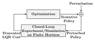
Figure 1: Schematic representation of the proposed strategy.

Using this information, EXP-LQR iteratively improves the policy taking on an extremum-seeking mechanism and a suitable reformulation of the LQR problem. This results in an overall algorithm that we interpret as a nonlinear time-varying system, which we then analyze by using system-theoretic tools based on the so-called averaging approach (see, for example, [44, Ch. 10] and [45] for the continuous-time case or [46] for the discrete-time one). Indeed, as customary in the context of averaging theory, we focus on the so-called averaged system associated to the algorithm. In particular, the averaged system reads as a policy gradient method perturbed by errors arising from the use of the truncated cost instead of the infinite-horizon one, as well as from the derivative-free gradient approximation. More in detail, we employ a Lyapunov-based approach to ensure that the averaged system trajectories exponentially converge to an arbitrarily small neighborhood of the optimal gain matrix. Then, we use this preparatory result to achieve the same property on the trajectories of the original time-varying algorithm. This final step is supported by Theorem 1, introduced in Section II, which presents averaging-related stability results for generic discrete-time systems. To the best of the authors’ knowledge, Theorem 1 also represents a per se contribution of this work. A conference version of this paper appeared in [47]. However, in that preliminary version, the algorithm relies on oracles providing the exact infinite-horizon cost associated to the tentative gain, making it impractical for real-world scenarios where only finite-time virtual or real experiments are feasible. Moreover, certain proofs were omitted. Finally, this work includes a concrete application example involving the control of an induction motor.

We organize the paper as follows. In Section II, we introduce some preliminaries about averaging theory for discrete-time systems. In Section III, we describe the problem setup considered in the paper. In Section IV, we provide the description of EXP-LQR and state its theoretical features. Finally, in Section V, we numerically test the effectiveness of EXP-LQR.

Notation

A square matrix $M\in\mathbb{R}^{n\times n}$ is Schur if all its eigenvalues lie in the open unit disk. The identity matrix in $\mathbb{R}^{n\times n}$ is $I_{n}$. The vector of zeros of dimension $n$ is denoted as $0_{n}$. The vertical concatenation of vectors $v_{1},\dots,v_{N}$ is $\operatorname{col}(v_{1},\dots,v_{N})$. Given $r>0$ and $x\in\mathbb{R}^{n}$, we use $\mathcal{B}_{r}(x)$ to denote the closed ball of radius $r>0$ centered in $x$, namely $\mathcal{B}_{r}(x):=\{y\in\mathbb{R}^{n}\mid\left\|y-x\right\|\leq r\}$. Given $A\in\mathbb{R}^{n\times n}$, $\operatorname{Tr}(A)$ denotes its trace. $\mathbb{R}_{+}$ denotes the positive orthant in $\mathbb{R}$.

II Preliminaries: Averaging Theory for Discrete-Time Systems

In this preliminary part, we provide a generic stability result for discrete-time systems in the context of averaging theory (see, e.g., [44, 45, 46]). Although we will use it as an instrumental step for proving the main result of the paper, we remark that it represents a contribution per se.

Let us consider the time-varying discrete-time system

$$\chi^{{k+1}}=\chi^{k}+\gamma f(\chi^{k},k)\qquad\chi^{0}=\chi_{0},$$ (1)

where $\chi^{k}\in\mathbb{R}^{n}$ denotes the state, $f:\mathbb{R}^{n}\times\mathbb{N}\to\mathbb{R}^{n}$ describes its dynamics, and $\gamma>0$ is a tunable parameter. Let us enforce the following assumptions.

Assumption 1.

There exist $\mathbf{k}_{\text{prd}}\in\mathbb{N}$ and $f_{\textsc{av}}\,:\,\mathbb{R}^{n}\to\mathbb{R}^{n}$ such that

$$f_{\textsc{av}}(\chi)=\dfrac{1}{\mathbf{k}_{\text{prd}}}\sum_{\tau=k+1}^{k+\mathbf{k}_{\text{prd}}}f(\chi,\tau),$$ (2)

for all $\chi\in\mathbb{R}^{n}$ and $k\in\mathbb{N}$. $\blacksquare$

Assumption 1 allows for properly writing a well-posed averaged system associated to system (1). Roughly, Assumption 1 says that $f(\chi,\cdot)$ is periodic and $\mathbf{k}_{\text{prd}}\in\mathbb{N}$ represents its period. The next assumption guarantees some regularity conditions on the functions $f$ and $f_{\textsc{av}}$ and their derivatives.

Assumption 2.

There exists a set $\mathcal{X}\subseteq\mathbb{R}^{n}$ such that the restrictions of $f(\cdot,k)$, $f_{\textsc{av}}(\cdot)$, $\partial f(\chi,k)/\partial\chi$, and $\partial f_{\textsc{av}}(\chi)/\partial\chi$ to $\mathcal{X}$ are continuous for all $k\in\mathbb{N}$. $\blacksquare$

The next assumption characterizes the convergence properties of the so-called averaged system associated to (1), i.e., the auxiliary time-invariant dynamics described by

$$\chi^{{k+1}}_{\textsc{av}}=\chi^{k}_{\textsc{av}}+\gamma f_{\textsc{av}}(\chi^{k}_{\textsc{av}})\qquad\chi^{0}_{\textsc{av}}=\chi_{0},$$ (3)

with $\chi^{k}_{\textsc{av}}\in\mathbb{R}^{n}$.

Assumption 3.

There exists $V:\mathcal{X}\to\mathbb{R}_{+}$ such that $V\in\mathcal{C}^{1}$ and, for any $c_{0}>0$ such that $\Omega_{c_{0}}\subseteq\mathcal{X}$ and any $\rho_{\textsc{av}}\in(0,c_{0})$, there exist $\bar{\gamma}_{1},a>0$ such that, for all $\chi_{0}\in\Omega_{c_{0}}$ and for all $\gamma\in(0,\bar{\gamma_{1}})$, it holds

$$V(\chi^{k}_{\textsc{av}})\leq V(\chi_{0})\exp(-\gamma ak),$$ (4)

along the trajectories of (3) and as long as $V(\chi^{k})\geq\rho_{\textsc{av}}$. $\blacksquare$

We are ready to state the following result about the original system (1).

Theorem 1.

Consider system (1) and let Assumptions 1-3 hold. Then, for any $c_{0},c_{1}>0$ such that $\Omega_{c_{0}}\subset\Omega_{c_{1}}\subseteq\mathcal{X}$ and $\rho\in(0,c_{0})$ there exist $\bar{\gamma}>0$ and $\bar{k}\in\mathbb{N}$ such that, for all $\chi_{0}\in\Omega_{c_{0}}$ and $\gamma\in(0,\bar{\gamma})$, it holds

$$V(\chi^{k})\leq c_{1},$$ (5)

for all $k\in\mathbb{N}$ and

$$V(\chi^{k})\leq\rho,$$ (6)

for all $k\geq\bar{k}$. Moreover, the convergence to $\Omega_{\rho}$ is exponentially fast. $\blacksquare$

The proof of Theorem 1 is provided in Appendix -A. Essentially, Theorem 1 ensures that, with sufficiently small values of the parameter $\gamma$, the properties of the averaged system (3) enforced by Assumption 3 can be “transferred” to the original time-varying system (1).

III Problem Setup

This section states the problem setup that we aim to address and recalls a model-based iterative approach to solve it.

III-A Data-Driven LQR Problem Setup

In this paper, we focus on LQR problems in the form

$$\min_{\begin{subarray}{c}x_{1},x_{2},\ldots,\\ u_{0},u_{1},\ldots\end{subarray}}\>\> \>\mathbb{E}\bigg{[}\frac{1}{2}\sum_{t=0}^{\infty}\Big{(}{x_{t}}^{\top}Qx_{t}+{u_{t}}^{\top}Ru_{t}\Big{)}\bigg{]}$$ (7a)

subj. to $$\>x_{{t+1}}=Ax_{t}+Bu_{t},\qquad\qquad x^{0}\sim\mathcal{X}^{0},$$ (7b)

where $x_{t}\in\mathbb{R}^{n}$ and $u_{t}\in\mathbb{R}^{m}$ denote, respectively, the state and the input of the system at time $t\in\mathbb{N}$, $A\in\mathbb{R}^{{n}\times{n}}$ and $B\in\mathbb{R}^{{n}\times{m}}$ represent the state and the input matrices, while $Q\in\mathbb{R}^{{n}\times{n}}$ and $R\in\mathbb{R}^{{m}\times{m}}$ are the cost matrices. As for the initial condition $x^{0}\in\mathbb{R}^{n}$, we assume that it is drawn from the uniform probability distribution $\mathcal{X}^{0}$ over the unitary-sphere. The operator $\mathbb{E}[\cdot]$ denotes the expected value with respect to $\mathcal{X}^{0}$. We require the following properties on the pairs $(A,B)$ and $(Q,R)$.

Assumption 4 (System and Cost Matrices Properties).

The pair $(A,B)$ is controllable, while the cost matrices $Q$ and $R$ are both symmetric and positive definite, i.e., $Q=Q^{\top}\succ 0$ and $R=R^{\top}\succ 0$. $\blacksquare$

Under the properties enforced by Assumption 4, when $(A,B)$ and $(Q,R)$ are known, the optimal solution to problem (7) is ruled by a linear time-invariant policy $u_{t}=K^{\star}x_{t}$ with $K^{\star}\in\mathbb{R}^{{m}\times{n}}$ given by

$$K^{\star}=-(R+B^{\top}P^{\star}B)^{-1}B^{\top}P^{\star}A,$$

where the matrix $P^{\star}\in\mathbb{R}^{{n}\times{n}}$ solves the so-called Discrete-time Algebraic Riccati Equation associated to problem (7), see [48]. However, as formalized in the next assumption, in this paper the knowledge of the pairs $(A,B)$ and $(Q,R)$ is not available and, therefore, $K^{\star}$ cannot be computed.

Assumption 5 (Unknown System and Cost Matrices).

The pairs $(A,B)$ and $(Q,R)$ are unknown. $\blacksquare$

Accordingly, we are interested in devising a data-driven strategy to iteratively address problem (7).

III-B Model-based Gradient Method for LQR

Next, we recall a model-based gradient method to address problem (7) in an iterative fashion. Let $\mathcal{K}\subset\mathbb{R}^{m\times n}$ be the set of stabilizing gains, namely

$$\mathcal{K}:=\{K\in\mathbb{R}^{m\times n}\mid A+BK\text{ is Schur}\}.$$

As shown in, e.g., [24], by considering the state-feedback control $u_{t}=Kx_{t}$ with $K\in\mathcal{K}$, it is possible to recast problem (7) as the unconstrained program

$$\min_{K\in\mathcal{K}}\> \>J(K),$$ (8)

where the cost function $J:\mathcal{K}\to\mathbb{R}$ is given by

$$J(K):=\tfrac{1}{2}\operatorname{Tr}\sum_{t=0}^{\infty}(A+BK)^{t,\top}(Q+K^{\top}RK)(A+BK)^{t}.$$

It is worth noting that since $x^{0}\sim\mathcal{X}^{0}$ (see problem (7)) and $\mathcal{X}^{0}$ is a uniform distribution over the unitary-radius sphere, then the set of stabilizing gains $\mathcal{K}$ coincides with the domain of the cost function $J$ [24]. Moreover, being the set $\mathcal{K}$ open [49, Lemma IV.3] and connected [49, Lemma IV.6], one could use the gradient descent method to iteratively solve problem (8) (see, e.g., [24]). Namely, at each iteration $k\in\mathbb{N}$, an estimate $K^{k}\in\mathbb{R}^{{n}\times{m}}$ of the optimal gain $K^{\star}$ could be maintained and iteratively updated according to

$$K^{{k+1}}=K^{k}-\gamma G(K^{k}),$$ (9)

where $\gamma>0$ is the step size parameter, while, when $\mathbb{R}^{m\times n}$ is equipped with the Frobenius inner product, $G:\mathbb{R}^{m\times n}\to\mathbb{R}^{m\times n}$ is the gradient of the cost function $J$ with respect to $K$ evaluated at $K^{k}$. In particular, given $K\in\mathcal{K}$, the gradient $G(K)$ reads as

$$G(K)=\left(RK+B^{\top}P(A+BK)\right)W_{c},$$

where the matrices $W_{c}\in\mathbb{R}^{n\times n}$ and $P\in\mathbb{R}^{n\times n}$ are solutions to the equations

$$(A+BK)W_{c}(A+BK)^{\top}-W_{c} =-I_{n}$$

$$(A+BK)^{\top}P(A+BK)-P =-(Q+{K}^{\top}RK).$$

Therefore, in our setup, it is not possible to compute $G(K^{k})$ and implement (9) because its computation would require the knowledge of the pairs $(A,B)$ and $(Q,R)$ that are both not available (cf. Assumption 5). However, for a given gain $K$ (e.g., the current estimate about the optimal gain $K^{\star}$), we assume the presence of an oracle providing the associated finite-horizon cost

$$J_{T}(K):=\tfrac{1}{2}\operatorname{Tr}\sum_{t=0}^{T-1}(A+BK)^{t,\top}(Q+K^{\top}RK)(A+BK)^{t},$$

where the number of samples $T\in\mathbb{N}$ represents an algorithm parameter that will be designed later. Differently from the entire cost $J(K)$ whose exact computation would require virtual or real experiments over infinite time horizons, we remark that $J_{T}(K)$ may be retrieved with finite-time virtual or real experiments using the control law $u_{t}=Kx_{t}$.

Remark 1.

We emphasize that the LQR problem (7) depends on the expectation over the system initial state $x^{0}$. However, since the latter is drawn from the uniform distribution $\mathcal{X}^{0}$ over the unitary sphere, the truncated cost $J_{T}(K)$ can be computed through ${n}$ virtual or real experiments each composed of $T$ samples of system (7b) controlled via $u_{t}=Kx_{t}$. In particular, the $i$-th experiment must be executed with $x^{0}=e_{i}$, where $e_{i}\in\mathbb{R}^{{n}}$ denotes the $i$-th vector of the canonical basis in $\mathbb{R}^{{n}}$. We also remark that retrieving $J_{T}(K)$ does not require measuring $x_{t}$, In particular, it can be obtained either measuring the output $y_{t}=x_{t}^{\top}Qx_{t}+u_{t}^{\top}Ru_{t}$ for $t\in\{0,\dots,T-1\}$ or having an oracle that directly provides the cumulative truncated cost $J_{T}(K)$ at the end of the experimental phase. $\blacksquare$

Our idea is to mimic (9) by elaborating these finite-horizon approximations $J_{T}(K)$ according to an extremum-seeking perspective to compensate for the lack of knowledge about the gradient $G(K)$.

IV EXP-LQR: Algorithm Description and Convergence Properties

In this section, we present EXtremum-seeking Policy iteration LQR (EXP-LQR), i.e., the novel data-driven method resumed in Algorithm 1 to iteratively address problem (7) without the knowledge of the system and cost matrices $(A,B)$ and $(Q,R)$.

Initialization: $\mathrm{z}^{0}\in\mathbb{R}$, $K^{0}\in\mathcal{K}$.

for $k=0,1,2\ldots$ do

     Experiment phase

         Set the controller $u_{t}=(K^{k}+\delta\mathrm{D}^{k})x_{t}$

         Test $x_{{t+1}}=Ax_{t}+Bu_{t}$ for $t=0,\dots,T-1$

         Retrieve $J_{T}(K^{k}+\delta\mathrm{D}^{k})$

     Optimization phase:

$$\mathrm{z}^{k+1} =\mathrm{z}^{k}+\gamma(J_{T}(K^{k}+\delta\mathrm{D}^{k})-\mathrm{z}^{k})$$ (10a)

$$K^{{k+1}} =K^{k}-\gamma\frac{2(J_{T}(K^{k}+\delta\mathrm{D}^{k})-\mathrm{z}^{k})\mathrm{D}^{k}}{\delta}$$ (10b)

end for

Algorithm 1 EXP-LQR

Our algorithmic idea is to mimic the (model-based) gradient descent update (9) through an extremum-seeking scheme. To this end, at each iteration $k$, we perturb a given policy gain $K^{k}$ obtaining $K^{k}+\delta\mathrm{D}^{k}$, where $\delta>0$ is an amplitude parameter and $\mathrm{D}^{k}\in\mathbb{R}^{m\times n}$ is the so-called dither matrix. The element $D_{ij}^{k}$ of $\mathrm{D}^{k}$ is generated according to the sinusoidal law

$$D_{ij}^{k}:=\sin\left(\frac{2\pi k}{\mathbf{k}_{ij,\text{prd}}}+\phi_{ij}\right),$$

where $\mathbf{k}_{ij,\text{prd}},\phi_{ij}\in\mathbb{R}$ are the period and the phase of component $(i,j)$, respectively, for all $(i,j)\in\{1,\ldots,{n}\}\times\{1,\ldots,{m}\}$. Such a perturbed policy is used to implement the feedback control law $u_{t}=(K^{k}+\delta\mathrm{D}^{k})x_{t}$ and retrieve the corresponding finite-horizon cost $J_{T}(K^{k}+\delta\mathrm{D}^{k})$ providing an approximation of the infinite-horizon one $J(K+\delta\mathrm{D}^{k})$. This scenario may occur, for example, when a simulator of a complex system is available, but the analytical knowledge of the dynamics being implemented for the simulations is unavailable. Hence, the finite-time truncation turns out to be crucial in avoiding experiments over infinite time horizons. With $J_{T}(K^{k}+\delta\mathrm{D}^{k})$ at hand, we perform the algorithm iteration detailed in (10). Specifically, the variable $\mathrm{z}^{k}\in\mathbb{R}$ filters the variation of $J_{T}(K^{k}+\delta\mathrm{D}^{k})$ (see its update (10a)), while the evolution of the gain matrix $K^{k}$ follows the extremum-seeking update (10b).

A block diagram representation that graphically describes EXP-LQR is provided in Fig. 2.

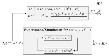
Figure 2: Block diagram representation of Algorithm 1.

Before establishing the convergence properties of EXP-LQR, we need to ensure that the dither matrix is generated by following the orthonormality conditions detailed in the next assumption.

Assumption 6 (Dither Frequencies Orthonormality).

Let $\mathbf{k}_{\text{prd}}\in\mathbb{N}$ be the least common multiple of all periods $\mathbf{k}_{11,\text{prd}},\dots,\mathbf{k}_{{m}{n},\text{prd}}$. Then, it holds

$$\sum_{k=1}^{\mathbf{k}_{\text{prd}}}\sin\left(\tfrac{2\pi k}{\mathbf{k}_{p,\text{prd}}}+\phi_{p}\right)\!=\!0$$ (11a)

$$\sum_{k=1}^{\mathbf{k}_{\text{prd}}}\sin\left(\tfrac{2\pi k}{\mathbf{k}_{p,\text{prd}}}+\phi_{p}\right)\sin\left(\tfrac{2\pi k}{\mathbf{k}_{q,\text{prd}}}+\phi_{q}\right)\!=\!\dfrac{\mathbf{k}_{\text{prd}}}{2}$$ (11b)

$$\sum_{k=1}^{\mathbf{k}_{\text{prd}}}\sin\!\left(\tfrac{2\pi k}{\mathbf{k}_{p,\text{prd}}}\!+\!\phi_{p}\right)\!\sin\!\left(\tfrac{2\pi k}{\mathbf{k}_{q,\text{prd}}}\!+\!\phi_{p}\right)\!\sin\!\left(\tfrac{2\pi k}{\mathbf{k}_{r,\text{prd}}}\!+\!\phi_{r}\right)\!=\!0,$$ (11c)

for all $p,q,r\in\{1,\ldots,{m}\}\times\{1,\ldots,{n}\}$ such that $p\neq q$, $q\neq r$, and $p\neq r$. $\blacksquare$

Now, we are in the position to provide the main result of the paper, i.e., the convergence properties of EXP-LQR.

Theorem 2 (Convergence Properties of EXP-LQR).

Consider EXP-LQR and let Assumptions 4, 5, and 6 hold. Then, for any $r>0$ and $(\mathrm{z}^{0},K^{0})\in\mathbb{R}\times\mathcal{K}$, there exist $\bar{\gamma},\bar{\delta}>0$ and $\bar{k},\bar{T}\in\mathbb{N}$, such that, for all $\gamma\in(0,\bar{\gamma})$, $\delta\in(0,\bar{\delta})$, $T\geq\bar{T}$, the trajectories of (10) are bounded and it holds

$$\left\|K^{k}-K^{\star}\right\|\leq r,$$ (12)

for all $k\geq\bar{k}$. Moreover, the convergence to the set $\{(\mathrm{z},K)\in\mathbb{R}\times\mathcal{K}\mid\left\|K-K^{\star}\right\|\leq r\}$ is exponentially fast. $\blacksquare$

The proof of Theorem 2 is provided in Section V-C. More in detail, the proof is based on the exploitation of Lyapunov stability and averaging theory tools to prove that $(\mathrm{z}^{\star},K^{\star})$ is a semi-global practical exponentially stable equilibrium point of system (10) restricted to $\mathbb{R}\times\mathcal{K}$, for a suitable $\mathrm{z}^{\star}\in\mathbb{R}$.

V Stability Analysis of EXP-LQR

In this section, we perform the stability analysis of system (10) to prove Theorem 2. First, in Section V-A, we perform a preliminary phase due to evaluate the approximation of the infinite-horizon gradient $G(K)$ using the finite-horizon cost $J_{T}(K)$. In Section V-B, by resorting to these approximations and an approach based on averaging theory, we characterize the stability and convergence properties of the so-called averaged system associated to (10). With these results at hand, in Section V-C, we come back to the original time-varying system (10) and provide the proof of Theorem 2. Assumptions 4, 5, and 6 are valid throughout the entire section.

V-A Preliminary Approximation Results

Here, we provide two approximation results that will be used in the remainder of the analysis of system (10). First, we evaluate the approximation error due to using the truncated cost $J_{T}(K\!+\!\delta\mathrm{D}^{k})$ instead of the infinite-horizon one $J(K\!+\!\delta\mathrm{D}^{k})$.

Lemma 1 (Truncated Cost Approximation Error).

For any $\alpha>0$ and compact set $\mathcal{S}\subset\mathcal{K}$, there exists $\bar{T}\in\mathbb{N}$ such that, for all $T\geq\bar{T}$, it holds

$$\|J(K)-J_{T}(K)\|\leq\alpha,$$ (13)

for all $K\in\mathcal{S}$. $\blacksquare$

The proof of Lemma 1 is provided in Appendix -B.

Second, we establish the gradient approximation properties obtained using the infinite-horizon cost samples $J(K+\mathrm{D}^{1}),\dots,J(K+\mathrm{D}^{\mathbf{k}_{\text{prd}}})$ for any fixed (and stabilizing) gain $K\in\mathcal{K}$.

Lemma 2 (Gradient Approximation Error).

For any compact set $\mathcal{S}\subset\mathcal{K}$, there exist $e:\mathbb{R}^{{m}\times{n}}\to\mathbb{R}^{{m}\times{n}}$ and $\beta_{e}>0$ such that

$$\dfrac{2}{\delta\mathbf{k}_{\text{prd}}}\!\!\sum_{\tau=k+1}^{k+\mathbf{k}_{\text{prd}}}\!\!\!J(K+\delta\mathrm{D}^{\tau})\mathrm{D}^{\tau} =G(K)+\delta^{2}e(K),$$ (14a)

$$\left\|e(K)\right\| \leq\beta_{e},$$ (14b)

for all $k\in\mathbb{N}$, $\delta\in(0,1]$, and $K$ such that $K+\delta\mathrm{D}^{\tau}\in\mathcal{S}$ for all $\tau\in\{1,\ldots,\mathbf{k}_{\text{prd}}\}$. $\blacksquare$

The proof of Lemma 2 is provided in Appendix -C.

With these results at hand, we are able to study the stability properties of system (10) through the averaging theory.

V-B Averaged System Analysis

As shown in Section II, the averaged system associated to (10) is an auxiliary dynamics derived by averaging the time-varying vector field of (10) over time horizons of length equal to the period $\mathbf{k}_{\text{prd}}$ (see Assumption 6). To properly write this system, given $K\in\mathcal{K}$ and $\mathrm{z}\in\mathbb{R}$, we consider the term $\sum_{\tau=k+1}^{k+\mathbf{k}_{\text{prd}}}(J_{T}(K+\delta\mathrm{D}^{\tau})-\mathrm{z})$ and add and subtract the infinite-horizon terms $J(K+\delta\mathrm{D}^{\tau})$ with $\tau=1,\dots,\mathbf{k}_{\text{prd}}$, thus obtaining

$$\sum_{\tau=k+1}^{k+\mathbf{k}_{\text{prd}}}(J_{T}(K+\delta\mathrm{D}^{\tau})-\mathrm{z})$$

$$=\sum_{\tau=k+1}^{k+\mathbf{k}_{\text{prd}}}(J(K+\delta\mathrm{D}^{\tau})-\mathrm{z})\mathrm{D}^{\tau}$$

$$\hskip 11.38092pt+\sum_{\tau=k+1}^{k+\mathbf{k}_{\text{prd}}}(J_{T}(K+\delta\mathrm{D}^{\tau})-J(K+\delta\mathrm{D}^{\tau}))\mathrm{D}^{\tau}$$

$$\stackrel{{\scriptstyle(a)}}{{=}}\sum_{\tau=k+1}^{k+\mathbf{k}_{\text{prd}}}J(K+\delta\mathrm{D}^{\tau})\mathrm{D}^{\tau}$$

$$\hskip 11.38092pt+\sum_{\tau=k+1}^{k+\mathbf{k}_{\text{prd}}}(J_{T}(K+\delta\mathrm{D}^{\tau})-J(K+\delta\mathrm{D}^{\tau}))\mathrm{D}^{\tau},$$ (15)

where in $(a)$ we used the frequencies’ property (11a) to simplify the expression. Hence, by applying Lemma 1, Lemma 2, and (15), the averaged system associated to (10) reads as

$$\mathrm{z}_{\textsc{av}}^{k+1} =\mathrm{z}_{\textsc{av}}^{k}+\gamma\left(J_{\textsc{av}}^{\delta}(K_{\textsc{av}}^{k})-\mathrm{z}_{\textsc{av}}^{k}\right)$$ (16a)

$$K_{\textsc{av}}^{{k+1}} =K_{\textsc{av}}^{k}-\gamma G(K_{\textsc{av}}^{k})+\gamma p^{\delta,T}(K_{\textsc{av}}^{k}),$$ (16b)

where $J_{\textsc{av}}^{\delta}:\mathcal{K}\to\mathbb{R}$ and $p^{\delta,T}:\mathcal{K}\to\mathcal{K}$ are defined as

$$J_{\textsc{av}}^{\delta}(K) :=\frac{1}{\mathbf{k}_{\text{prd}}}\sum_{\tau=k+1}^{k+\mathbf{k}_{\text{prd}}}J_{T}(K+\delta\mathrm{D}^{\tau})$$ (17a)

$$p^{\delta,T}(K) :=-\dfrac{2}{\delta\mathbf{k}_{\text{prd}}}\!\!\sum_{\tau=k+1}^{k+\mathbf{k}_{\text{prd}}}\!\!\!\left(J_{T}(K\!+\!\delta\mathrm{D}^{\tau})\!-\!J(K\!+\!\delta\mathrm{D}^{\tau})\right)\mathrm{D}^{\tau}\!$$

$$\hskip 11.38092pt-\delta^{2}e(K).$$ (17b)

As graphically highlighted in Fig. 3, we remark that the averaged scheme (16) is a cascade system.

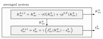
Figure 3: Block diagram representation of the averaged system (16).

The next lemma provides the convergence properties of the averaged system (16). To this end, we introduce the candidate Lyapunov function $V:\mathbb{R}\times\mathcal{K}\to\mathbb{R}_{+}$ defined as

$$V_{\lambda}(\mathrm{z},K) :=\frac{1}{2\lambda}\left\|\mathrm{z}\right\|^{2}+J(K)-J(K^{\star}),$$ (18)

where $\lambda\geq 1$ will be fixed in the next lemma.

Lemma 3 (Averaged System Stability).

Consider (16). Then, for all $(\mathrm{z}_{\textsc{av}}^{0},K_{\textsc{av}}^{0})\in\mathbb{R}\times\mathcal{K}$ and $\rho_{\textsc{av}}>0$, there exist $\bar{\gamma}_{1},\bar{\delta}_{1},a,\bar{T}>0$ and $\bar{\lambda}\geq 1$ such that, for all $\gamma\in(0,\bar{\gamma}_{1})$, $\delta\in(0,\bar{\delta}_{1})$, $T\geq\bar{T}$, and $\lambda\geq\bar{\lambda}$, it holds

$$V_{\lambda}(\mathrm{z}_{\textsc{av}}^{k}-J_{\textsc{av}}^{\delta}(K_{\textsc{av}}^{k}),K_{\textsc{av}}^{k})$$

$$\leq\exp(-\gamma ak)V_{\lambda}(\mathrm{z}_{\textsc{av}}^{0}-J_{\textsc{av}}^{\delta}(K_{\textsc{av}}^{0}),K_{\textsc{av}}^{0}),$$ (19)

for all $V_{\lambda}(\mathrm{z}_{\textsc{av}}^{k}-J_{\textsc{av}}^{\delta}(K_{\textsc{av}}^{k}),K_{\textsc{av}}^{k})\geq\rho_{\textsc{av}}$. $\blacksquare$

The proof of Lemma 3 is provided in Appendix -D.

V-C Proof of Theorem 2

The proof relies on the application of Theorem 1 (cf. Section II) to system (10). Then, in order to apply Theorem 1, we need to (i) choose the design parameters $c_{1},\rho>0$ bounding the initial and final values of $V_{\lambda}$, respectively, and (ii) satisfy the conditions required by Assumptions 1, 2, and 3. By [50, Lemma 3.8], we recall that there exists $\psi>0$ such that

$$\psi\left\|K-K^{\star}\right\|\leq J(K)-J(K^{\star}),$$ (20)

for all $K\in\mathcal{K}$. Therefore, by looking at the statement of Theorem 1 and given the desired final radius $r$, we set $\rho\in(0,r\psi]$. In order to set the initial radius, we need to find a bound for $\delta$ such that $K^{0}+\delta\mathrm{D}^{k}$ is stabilizing for all $k\in\mathbb{N}$. To this end, we note that $K^{0}\in\mathcal{K}$, $\mathcal{K}$ is open [49, Lemma IV.3], and $\mathrm{D}^{k}$ is bounded for all $k\in\mathbb{N}$. Hence, there exists $\bar{\delta}_{0}>0$ such that $K^{0}+\delta\mathrm{D}^{k}\in\mathcal{K}$ for all $\delta\in[0,\bar{\delta}]$ and $k\in\{1,\ldots,\mathbf{k}_{\text{prd}}\}$. Now, we arbitrarily choose $c_{1}>\max_{\delta\in[0,\bar{\delta}_{0}]}V_{1}(\mathrm{z}^{0}-J_{\textsc{av}}^{\delta}(K^{0}),K^{0})$ and, thus, we note that $c_{1}\geq\max_{\delta\in[0,\bar{\delta}]}V_{\lambda}(\mathrm{z}^{0}-J_{\textsc{av}}^{\delta}(K^{0}),K^{0})$ for all $\lambda\geq 1$ (see the definition of $V_{\lambda}$ in (18)). Once the initial and final radius $c_{1}$ and $\rho$ have been chosen, let us check Assumptions 1, 2, and 3. First, Assumption 1 is trivially satisfied because the dither signals are $\mathbf{k}_{\text{prd}}$-periodic (cf. Assumption 6). Second, we remark that (10) and its corresponding averaged system (16) are continuous over the set $\{(\mathrm{z},K)\in\mathbb{R}\times\mathcal{K}\mid K+\delta\mathrm{D}^{k}\in\mathcal{K}\text{ for all }k\in\mathbb{N}\}$, as required by Assumption 2. For this reason, let us choose $\delta$ such that the level set $\Omega_{c_{1}}:=\{(\mathrm{z},K)\in\mathbb{R}\times\mathcal{K}\mid V_{1}(\mathrm{z}-J_{\textsc{av}}^{\delta}(K),K)\leq c_{1}\}$ of $V_{1}$ (i.e, the function $V_{\lambda}$ with $\lambda=1$, see (18)) is contained into $\{(\mathrm{z},K)\in\mathbb{R}\times\mathcal{K}\mid K+\delta\mathrm{D}^{k}\in\mathcal{K}\text{ for all }k\in\mathbb{N}\}$. To this end, by looking at the definition of $V_{\lambda}$ (cf. (18)), we note that

$$V_{1}(\mathrm{z}-J_{\textsc{av}}^{\delta}(K),K)\leq c_{1}\implies J(K)-J(K^{\star})\leq c_{1},$$ (21)

independently on the choice of $\delta$. In turn, the result (21) implies

$$(\mathrm{z},K)\in\Omega_{c_{1}}\implies K\in\mathcal{K}.$$

Moreover, we recall that $\mathcal{K}$ is open [49, Lemma IV.3] and $\mathrm{D}^{k}$ is bounded for all $k\in\mathbb{N}$. Then, we guarantee the existence of $\bar{\delta}_{2}>0$ such that, for all $\delta\in(0,\min\{\bar{\delta}_{0},\bar{\delta}_{2}\})$, it holds $K+\delta\mathrm{D}^{k}\in\mathcal{K}$ for all $K$ satisfying $J(K)-J(K^{\star})\leq c_{1}$ and $k\in\mathbb{N}$. With these results at hand, Lemma 3 ensures the existence of $\bar{\gamma}_{1},\bar{\delta}_{1}>0$, $\bar{\lambda}\geq 1$, and $\bar{T}\in\mathbb{N}$ such that, by setting $\gamma\in(0,\bar{\gamma}_{1})$, $\delta\in(0,\bar{\delta})$ with $\bar{\delta}:=\min\{\bar{\delta}_{0},\bar{\delta}_{1},\bar{\delta}_{2}\}$, $T>\bar{T}$ and $\lambda\geq\bar{\lambda}$, $V_{\lambda}$ achieves the convergence properties (19) along the trajectories of the averaged system (16) and, thus, Assumption 3 is satisfied. Hence, we are entitled to apply Theorem 1. Specifically, it ensures the existence of $\bar{\gamma},\bar{k}>0$ such that, for all $\gamma\in(0,\bar{\gamma})$ and $k\geq\bar{k}$, it holds

$$V_{\lambda}(\mathrm{z}^{k}-J(K^{k}),K^{k})\leq\rho,$$ (22)

for all $(\mathrm{z}^{0},K^{0})\in\Omega_{c_{1}}$. The proof of (12) follows by combining $J(K)-J(K^{\star})\leq V(\mathrm{z}-J(K),K)$, (20), (22), and the choice of $\rho$.

VI Numerical Simulations: Control of a Doubly Fed Induction Motor

In this section, we numerically test the effectiveness of EXP-LQR. To this end, we consider a forward Euler discretization of the continuous-time linear model provided by [51] for a Doubly Fed Induction Motor (DFIM) operating at constant speed. Namely, we consider the discrete-time linear system

$$x_{{t+1}}=\underbrace{(I+\Delta tA_{\text{cont}})}_{A}x_{t}+\underbrace{\Delta tB_{\text{cont}}}_{B}u_{t},$$ (23)

where $\Delta t=10^{-2}$ is the adopted sampling period, while $x,u\in\mathbb{R}^{4}$ are the state and input variables, respectively, and are defined as

$$x:=\begin{bmatrix}i_{1u}\\ i_{1v}\\ i_{2u}\\ i_{2v}\end{bmatrix},\quad u:=\begin{bmatrix}u_{1u}\\ u_{1v}\\ u_{2u}\\ u_{2v}\end{bmatrix},$$

where $i_{1u},i_{1v}\in\mathbb{R}$ are the stator currents and $i_{2u},i_{2v}\in\mathbb{R}$ are the rotor currents, while $u_{1u},u_{1v}\in\mathbb{R}$ are the stator voltages and $u_{2u},u_{2v}\in\mathbb{R}$ the rotor voltages. Finally, $A_{\text{cont}}\in\mathbb{R}^{4\times 4}$ and $B_{\text{cont}}\in\mathbb{R}^{4\times 4}$ represent the state and input matrices of the continuous-time model, respectively, and are defined as

$$A_{\text{cont}} :=\frac{1}{\bar{L}}\begin{bmatrix}-L_{2}R_{1}&-a+b&L_{m}R_{2}&b_{2}\\ a-b&-L_{2}R_{1}&-b_{2}&-L_{m}R_{2}\\ L_{m}R_{1}&-b_{1}&-L_{1}R_{2}&-a-b_{12}\\ b_{1}&L_{m}R_{1}&a+b_{12}&-L_{1}R_{2}\end{bmatrix}$$

$$B_{\text{cont}} :=\frac{1}{\bar{L}}\begin{bmatrix}L_{2}&0&-L_{m}&0\\ 0&L_{2}&0&-L_{m}\\ -L_{m}&0&L_{1}&0\\ 0&-L_{m}&0&L_{1}\end{bmatrix},$$

where

$$\bar{L} \coloneqq L_{1}L_{2}-L_{m}^{2},\quad a:=\bar{L}\omega_{0},\quad b\coloneqq L_{m}^{2}\omega_{r}$$

$$b_{12} :=L_{1}L_{2}\omega_{r},\quad b_{1}\coloneqq L_{1}L_{m}\omega_{r},\quad b_{2}\coloneqq L_{2}L_{m}\omega_{r}.$$

More in detail, the parameters $R_{1}$ and $R_{2}$ correspond to the resistances of the stator and rotor, while the parameters $L_{1}$, $L_{2}$, and $L_{m}$ refer to the stator and rotor self-inductances, and the mutual inductance, respectively. Lastly, $\omega_{r}$ and $\omega_{0}$ denote the electrical angular velocities of the rotor and the rotating reference frame, respectively, which are assumed constant. We adopt the physical parameters used by [33] about the same model, and we report them in Table I. These parameters make the discrete-time pair $(A,B)$ controllable as required by Assumption 4.

TABLE I: Physical parameters of the DFIM [33].

Parameter	Value	Parameter	Value
$L_{1}$ [htpb]	$0.02645$	$R_{1}$ [$\Omega$]	$0.036$
$L_{2}$ [htpb]	$0.0264$	$R_{2}$ [$\Omega$]	$0.038$
$L_{m}$ [htpb]	$0.0257$	$\omega_{0}$ [rad/s]	$2\pi 70.8$
$p$	$3$	$\omega_{r}$ [rad/s]	$2\pi 62$

For the cost matrices $Q\in\mathbb{R}^{4\times 4}$ and $R\in\mathbb{R}^{4\times 4}$, we randomly generate them to ensure they are symmetric, with eigenvalues lying within the interval $(0,2)$ thus satisfying Assumption 4.

We arbitrarily pick $T=20$, i.e., the algorithm needs to perform $4$ experiments or simulations given by $20$ samples per iteration to retrieve the truncated cost $J_{T}(K^{k}+\delta\mathrm{D}^{k})$, see Remark 1. We empirically tune the other algorithm parameters as $\gamma=10^{-8}$ and $\delta=10^{-2}$. As for the generation of the dither matrix $\mathrm{D}^{k}\in\mathbb{R}^{4\times 4}$, we ordered the pairs $(i,j)\in\{1,\ldots,4\}\times\{1,\ldots,4\}$ with indices $p=1,\dots,16$ and chosen $\mathbf{k}_{p,\text{prd}}=19^{-(p-1)/2}$ and $\phi_{p}=0$ for $p$ odd, while $\mathbf{k}_{p,\text{prd}}=\mathbf{k}_{p-1,\text{prd}}$ and $\phi_{p}=\pi/2$ for $p$ even. This choice ensures that Assumption 6 is satisfied with period $\mathbf{k}_{\text{prd}}=19$.

Fig. 4 shows the evolution of the relative cost error $(J(K^{k})-J(K^{\star}))/J(K^{\star})$ along the algorithm iterations $k$ in logarithmic scale. As predicted by Theorem 2, Fig. 4 shows that EXP-LQR asymptotically converges in a neighborhood of the optimal gain $K^{\star}$.

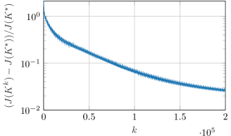
Figure 4: Evolution of the relative cost error $(J(K^{k})-J(K^{\star}))/J(K^{\star})$ along the algorithm iteration $k$.

In Fig. 5, we show the evolution of $\sigma_{\text{max}}(A+B(K^{k}+\delta\mathrm{D}^{k}))$ along the algorithm iterations $k$, where, given a generic square matrix $M\in\mathbb{R}^{n\times n}$, the symbol $\sigma_{\text{max}}(M)$ denotes the maximum (in absolute value) eigenvalue of $M$. In particular, Fig. 5 shows that $\sigma_{\text{max}}(A+B(K^{k}+\delta\mathrm{D}^{k}))$ never reaches the unitary value, i.e., we always test the system through a stabilizing state-feedback controller $u_{t}=(K^{k}+\delta\mathrm{D}^{k})x_{t}$.

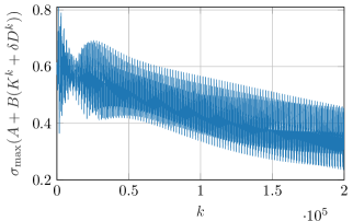
Figure 5: Evolution of the maximum (in absolute value) closed-loop matrix eigenvalue $\sigma_{\text{max}}(A+B(K^{k}+\delta\mathrm{D}^{k}))$ along the algorithm iteration $k$.

Finally, in Fig. 6, we show the evolution of the norm of the state trajectory $\left\|x_{t}\right\|$ of system (23) in four simulations (each composed of $T=20$ samples) performed at different algorithm iterations $k$ to retrieve the truncated cost $J_{T}(K^{k}+\delta\mathrm{D}^{k})$. In particular, Fig. 6 shows that the trajectories of system (23) (controlled with $u_{t}=(K^{k}+\delta\mathrm{D}^{k})u_{t}$) exponentially converge to the origin quicker and quicker as the iteration index $k$ increases since we are iteratively reducing the absolute values of the eigenvalues of the gain closed-loop matrix $(A+BK^{k})$ (see also Fig. 5).

(a)

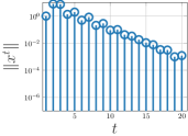
(b)

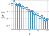
(c)

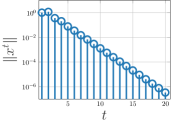
(d)

Figure 6: System evolutions in the interval $[0,T]$ along different algorithm iterations $k$.

VII Conclusions

We proposed EXP-LQR, i.e., a novel data-driven method able to iteratively find the state feedback gain matrix solving a Linear Quadratic Regulator problem. EXP-LQR does not need the direct knowledge of the system matrices, cost matrices, and state measurements. Indeed, given an oracle able to provide a finite-time truncation of the LQR cost, our method refines its estimate according to a mechanism based on extremum-seeking. We analyzed the resulting time-varying algorithm by exploiting system theory tools based on Lyapunov stability and averaging theory. Specifically, we guaranteed that our algorithm exponentially converges to an arbitrarily small ball containing the optimal gain matrix. We tested the proposed solution with numerical simulations involving the control of an inductance motor.

-A Proof of Theorem 1

Since Assumption 3 characterizes the evolution of $V$ along the trajectories $\{\chi^{k}_{\textsc{av}}\}_{k\in\mathbb{N}}$ of the averaged system (16), the idea of the proof is to bound the distance $\|\chi^{k}-\chi^{k}_{\textsc{av}}\|$ to characterize the evolution of $V$ along the trajectories $\{\chi^{k}\}_{k\in\mathbb{N}}$ of the original time-varying system (1). To this end, we introduce $\upsilon:\mathbb{R}^{n}\times\mathbb{N}\to\mathbb{R}^{n}$ defined as

$$\upsilon(\chi_{\textsc{av}},k):=\sum_{\tau=0}^{k-1}\left(f(\chi_{\textsc{av}},\tau)-f_{\textsc{av}}(\chi_{\textsc{av}})\right).$$ (24)

By using (2) and (24), the evolution of $\upsilon$ reads as

$$\upsilon(\chi^{{k+1}}_{\textsc{av}},{k+1})-\upsilon(\chi^{k}_{\textsc{av}},k)$$

$$=f(\chi^{{k+1}}_{\textsc{av}},k)-f_{\textsc{av}}(\chi^{{k+1}}_{\textsc{av}})+\upsilon(\chi^{{k+1}}_{\textsc{av}},k)-\upsilon(\chi^{k}_{\textsc{av}},k).$$ (25)

Let us recall that $V(\chi_{0})\leq c_{0}$ and that $\rho<c_{0}<c_{1}$ by assumption. Then, let us arbitrarily choose $\epsilon\in(0,\min\{c_{1}-c_{0},\rho\})$, and $\rho_{\textsc{av}}\in(0,\min\{\rho-\epsilon,c_{0}\})$. As it will become clearer later, $\epsilon$ represents the maximum difference between $V(\chi^{k})$ and $V(\chi^{k}_{\textsc{av}})$, where $\rho_{\textsc{av}}$ defines the level set of $V$ in which we enforce the convergence of the averaged state $\chi^{k}_{\textsc{av}}$. (cf. Assumption 3). Under the assumption of $\chi^{k}\in\Omega_{c_{1}}$ for all $k\in\mathbb{N}$ (later verified by a proper selection of $\gamma$), we use the compactness of the set $\Omega_{c_{1}}$ (cf. Assumption 3) and the continuity properties over $\Omega_{c_{1}}\subseteq\mathcal{X}$ (cf. Assumption 2) to ensure the existence of $L>0$ such that

$$\left\|f(\chi,k)\right\| \leq L$$ (26a)

$$\left\|f_{\textsc{av}}(\chi)\right\| \leq L$$ (26b)

$$\left\|\dfrac{\partial f(\chi,k)}{\partial\chi}\right\| \leq L$$ (26c)

$$\left\|\nabla f_{\textsc{av}}(\chi)\right\| \leq L$$ (26d)

$$\left\|\nabla V(\chi)\right\| \leq L,$$ (26e)

for all $\chi\in\Omega_{c_{1}}$ and $k\in\mathbb{N}$. In turn, the bounds (26) lead to

$$\left\|\upsilon(\chi,k)\right\| \leq 2L\mathbf{k}_{\text{prd}}$$ (27a)

$$\left\|f(\chi,k)-f(\chi^{\prime},k)\right\| \leq L\left\|\chi-\chi^{\prime}\right\|$$ (27b)

$$\left\|f_{\textsc{av}}(\chi)-f_{\textsc{av}}(\chi^{\prime})\right\| \leq L\left\|\chi-\chi^{\prime}\right\|$$ (27c)

$$\left\|\upsilon(\chi,k)-\upsilon(\chi^{\prime},k)\right\| \leq 2L\mathbf{k}_{\text{prd}}\left\|\chi-\chi^{\prime}\right\|$$ (27d)

$$\left\|f_{\textsc{av}}(\chi)\right\| \leq L$$ (27e)

$$V(\chi)-V(\chi^{\prime}) \leq L,$$ (27f)

for all $\chi,\chi^{\prime}\in\Omega_{c_{1}}$ and $k\in\mathbb{N}$. Now, let us introduce $\zeta^{k}\in\mathbb{R}^{n}$ defined as

$$\zeta^{k}:=\chi^{k}_{\textsc{av}}+\gamma\upsilon(\chi^{k}_{\textsc{av}},k).$$ (28)

By algebraically rearranging the terms, we can write

$$\chi^{k}-\zeta^{k} =\sum_{\tau=0}^{k-1}\left((\chi^{\tau+1}-\chi^{\tau})-(\zeta^{\tau+1}-\zeta^{\tau})\right).$$

Now let us add $\pm\gamma\sum_{\tau=0}^{k-1}(f(\zeta^{\tau},\tau)+f(\chi^{\tau}_{\textsc{av}},\tau))$ in the above equation and use (25) to get

$$\chi^{k}-\zeta^{k} =\gamma\sum_{\tau=0}^{k-1}(f(\chi^{\tau},\tau)-f(\zeta^{\tau},\tau))$$

$$\hskip 11.38092pt+\gamma\sum_{\tau=0}^{k-1}(f(\zeta^{\tau},\tau)-f(\chi^{\tau}_{\textsc{av}},\tau))$$

$$\hskip 11.38092pt-\gamma\sum_{\tau=0}^{k-1}(f(\chi^{\tau+1}_{\textsc{av}},\tau)-f(\chi^{\tau}_{\textsc{av}},\tau))$$

$$\hskip 11.38092pt+\gamma\sum_{\tau=0}^{k-1}(f_{\textsc{av}}(\chi^{\tau+1}_{\textsc{av}})-f_{\textsc{av}}(\chi^{\tau}_{\textsc{av}}))$$

$$\hskip 11.38092pt-\gamma\sum_{\tau=0}^{k-1}(\upsilon(\chi^{\tau+1}_{\textsc{av}},\tau)-\upsilon(\chi^{\tau}_{\textsc{av}},\tau)).$$ (29)

By combining (29) with (1), (3), and (27), we can write

$$\left\|\chi^{k}-\zeta^{k}\right\|\leq\gamma L\sum_{\tau=0}^{k-1}\left\|\chi^{k}-\zeta^{\tau}\right\|+\gamma^{2}L^{2}2\left(1+2\mathbf{k}_{\text{prd}}\right)k.$$ (30)

Note that

$$\sum_{\tau=0}^{k-1}\gamma Lk\exp\left(-\gamma Lk\right)\leq\sum_{\tau=0}^{\infty}\gamma L\tau\exp\left(-\gamma L\tau\right)=1.$$ (31)

By combining (31) and the discrete Gronwall inequality (see [52, 53]), we are able to bound (30) as

$$\left\|\chi^{k}-\zeta^{k}\right\|\leq \,\gamma^{2}L^{2}2\left(1+2\mathbf{k}_{\text{prd}}\right)k+\gamma L2\left(1+2\mathbf{k}_{\text{prd}}\right)\exp\left(\gamma Lk\right)\!.$$

By combining the latter with the definition of $\zeta$ (cf. (28)) and the triangle inequality, we get

$$\left\|\chi^{k}-\chi^{k}_{\textsc{av}}\right\| \leq\gamma^{2}L^{2}2\left(1+2\mathbf{k}_{\text{prd}}\right)k$$

$$\hskip 11.38092pt+\gamma L2\left(1+2\mathbf{k}_{\text{prd}}\right)\exp\left(\gamma Lk\right)+\gamma\left\|\upsilon(k,\chi^{k}_{\textsc{av}})\right\|$$

$$\stackrel{{\scriptstyle(a)}}{{\leq}}\gamma^{2}L^{2}2\left(1+2\mathbf{k}_{\text{prd}}\right)k$$

$$\hskip 11.38092pt+\gamma L2\left(1+2\mathbf{k}_{\text{prd}}\right)\exp\left(\gamma Lk\right)\!+\!\gamma 2L\mathbf{k}_{\text{prd}}.\!\!$$ (32)

where in $(a)$ we use (27a) to bound $\left\|\upsilon(k,\chi^{k}_{\textsc{av}})\right\|$. Then, we set $\theta_{\rho_{\textsc{av}}}\in\mathbb{R}$ such that

$$\theta_{\rho_{\textsc{av}}}\geq-\frac{1}{a}\ln\left(\tfrac{\rho_{\textsc{av}}}{c_{0}}\right).$$ (33)

Now, we want to impose the $\epsilon$-closeness between the trajectories of system (1) and its averaged version (3). To this end, by looking at the bound in (32), we introduce

$$\bar{\gamma}_{2} :=\tfrac{\epsilon/(3L)}{L^{2}2\left(1+2\mathbf{k}_{\text{prd}}\right)\theta_{\rho_{\textsc{av}}}}$$ (34a)

$$\bar{\gamma}_{3} :=\tfrac{\epsilon/(3L)}{2L(1+2\mathbf{k}_{\text{prd}})\exp(L\theta_{\rho_{\textsc{av}}})}$$ (34b)

$$\bar{\gamma}_{4} :=\tfrac{\epsilon/(3L)}{2L\mathbf{k}_{\text{prd}}}$$ (34c)

$$\bar{\gamma}_{1} :=\min\{\bar{\gamma}_{2},\bar{\gamma}_{3},\bar{\gamma}_{4}\}.$$ (34d)

Subsequently, we pick $\gamma\in(0,\bar{\gamma}_{1})$ such that $\bar{k}:=\frac{\theta_{\rho_{\textsc{av}}}}{\gamma}\in\mathbb{N}$. This can be done without loss of generality since $\theta_{\rho_{\textsc{av}}}$ is a design parameter. Then, the definition of $\bar{\gamma}_{1}$ (cf. (34d)) and the inequality in (32) lead to the bound

$$\left\|\chi^{k}-\chi^{k}_{\textsc{av}}\right\|\leq\frac{\epsilon}{L},$$ (35)

for all $k\in\{0,\dots,\bar{k}\}$. Then, for all $k\in\{0,\dots,\bar{k}\}$, we add and subtract $V(\chi^{k}_{\textsc{av}})$ to $V(\chi^{k})$ and write

$$V(\chi^{k}) =V(\chi^{k}_{\textsc{av}})+V(\chi^{k})-V(\chi^{k}_{\textsc{av}})$$

$$\stackrel{{\scriptstyle(a)}}{{\leq}}c_{0}+L\left\|\chi^{k}-\chi^{k}_{\textsc{av}}\right\|$$

$$\stackrel{{\scriptstyle(b)}}{{\leq}}c_{0}+\epsilon$$

$$\stackrel{{\scriptstyle(c)}}{{\leq}}c_{1},$$ (36)

where in $(a)$ we use the fact that $\chi^{k}_{\textsc{av}}\in\Omega_{c_{0}}$ for all $k\geq 0$ (see (4) by Assumption 3) and the bound (27f), in $(b)$ we use the bound (35), while in $(c)$ we use the fact that $\epsilon\leq c_{1}-c_{0}$. Therefore, the bound (36) allows us to claim that

$${\chi}^{k}\in\Omega_{c_{1}},$$

for all $k\in\{0,\dots,\bar{k}\}$, i.e., we have verified that the bounds (27) can be used into the interval $\{0,\dots,\bar{k}\}$. Moreover, the exponential law (4) and the expression of $\theta_{\rho_{\textsc{av}}}$ (cf. (33)) ensure that it holds

$$V(\chi^{k}_{\textsc{av}})\leq\rho_{\textsc{av}},$$ (37)

for all $k\geq\bar{k}$. By adding and subtracting $V(\chi^{\bar{k}}_{\textsc{av}})$ to $V(\chi^{k})$, we get

$$V(\chi^{\bar{k}}) =V(\chi^{\bar{k}}_{\textsc{av}})+V(\chi^{\bar{k}})-V(\chi^{\bar{k}}_{\textsc{av}})$$

$$\stackrel{{\scriptstyle(a)}}{{\leq}}\rho_{\textsc{av}}+L\left\|\chi^{\bar{k}}-\chi^{\bar{k}}_{\textsc{av}}\right\|$$

$$\stackrel{{\scriptstyle(b)}}{{\leq}}\rho_{\textsc{av}}+\epsilon$$

$$\stackrel{{\scriptstyle(c)}}{{\leq}}\rho,$$ (38)

where in $(a)$ we combined (27f) and (37), in $(b)$ we used (35), while $(c)$ uses the choice of $\rho_{\textsc{av}}\leq\rho-\epsilon$. We remark that the inequality (38) also guarantees that $\chi^{\bar{k}}\in\Omega_{c_{0}}$ since $\rho\leq c_{0}$. Next, in order to show that $\chi^{k}\in\Omega_{\rho}$ for all $k\geq\bar{k}$, we divide the set of natural numbers in intervals as $\mathbb{N}=\{0,\dots,\bar{k}\}\cup\{\bar{k},\dots,2\bar{k}\}\cup\dots$. Define $\psi_{\textsc{av}}(\chi^{\bar{k}},k+\bar{k})$ as the solution to (3) for $\chi^{0}_{\textsc{av}}=\chi^{\bar{k}}$ and $k\in\{0,\dots,\bar{k}\}$. Thus, at the beginning of the time interval $\{\bar{k},\dots,2\bar{k}\}$, the initial condition of the trajectory of (3) coincides with the one of $\psi_{\textsc{av}}(\chi^{\bar{k}},k+\bar{k})$ and lies into $\Omega_{\rho}\subseteq\Omega_{c_{0}}$. Thus, we apply the same arguments above to guarantee that, for any $\gamma\in(0,\bar{\gamma})$, it holds

$$\left\|\chi^{k+\bar{k}}-\psi_{\textsc{av}}(\chi^{\bar{k}},k+\bar{k})\right\|\leq\frac{\epsilon}{L},$$

for all $k\in\{0,\dots,\bar{k}\}$. Moreover, with the same arguments, it holds $\psi_{\textsc{av}}(\chi^{\bar{k}},2\bar{k})\in\Omega_{\rho_{\textsc{av}}}$. Then, in light of Assumption 3, we guarantee that the averaged system (3) cannot escape from the set $\Omega_{\rho}$, namely

$$\chi^{k}_{\textsc{av}}\in\Omega_{\rho},$$

for all $k\in\{\bar{k},\dots,2\bar{k}\}$. Thus, we get $\chi^{k}\in\Omega_{\rho}$ for all $k\in\{\bar{k},\dots,2\bar{k}\}$. The proof follows by recursively applying the above arguments for each time interval $\{j\bar{k},\dots,(j+1)\bar{k}\}$ with $j=2,3,\dots$.

-B Proof of Lemma 1

We observe that

$$\lim_{T\to\infty}J_{T}(K)=J(K),$$

for all $K\in\mathcal{S}\subset\mathcal{K}$. Therefore, since the series of real numbers $\{J_{T}(K)\}_{T\in\mathbb{N}}$ converges to $J(K)$ and $J(K)$ is finite since $K\in\mathcal{K}$ by assumption, we can exploit the Cauchy convergence criterion to demonstrate that, for any $\alpha>0$ and $\mathcal{S}\in\mathcal{K}$, there exists a finite $\bar{T}\in\mathbb{N}$, possibly function of $\alpha$ and $\mathcal{S}$, such that for any $T>\bar{T}$, the bound (13) is achieved and the proof concludes.

-C Proof of Lemma 2

We note that [54, Lemma 1] provides the same results claimed in Lemma 2. The only difference is that, in the mentioned reference, the objective function is assumed to have globally Lipschitz gradients. However, since we assumed compactness of the set $\mathcal{S}\subset\mathcal{K}$ and since $J$ and its gradient $G$ are continuous and differentiable [24] over the set of stabilizing gains $\mathcal{K}$, the constant

$$\beta_{\mathcal{S}} :=\max_{K\in\mathcal{S}}\left\|\nabla G(K)\right\|,$$

is finite, and we can use it as Lipschitz constant of $G$ over $\mathcal{S}$. With this constant at hand, we can repeat all the steps in [54, Lemma 1] to conclude the proof.

-D Proof of Lemma 3

Let us start by using the cost $J$ to introduce the function $V_{K}:\mathcal{K}\to\mathbb{R}$ defined as

$$V_{K}(K_{\textsc{av}}):=J(K_{\textsc{av}})-J(K^{\star}).$$ (39)

Being $K^{\star}$ the unique minimizer of $J$ [24], we note that $V_{K}$ is positive definite. Now, given any $c>0$, let us introduce

$$\tilde{\Omega}_{c}\! :=\!\Big{\{}(\mathrm{z}_{\textsc{av}},K_{\textsc{av}})\in\mathbb{R}\times\mathcal{K}\mid$$

$$\hskip 25.8921pt\tfrac{1}{2}\left\|\mathrm{z}_{\textsc{av}}\!-\!J_{\textsc{av}}^{\delta}(K_{\textsc{av}})\right\|^{2}\!+\!J(K_{\textsc{av}})\!-\!J(K^{\star})\!\leq\!c\Big{\}}$$ (40a)

$$\Omega^{K}_{c}\! :=\!\Big{\{}K_{\textsc{av}}\in\mathcal{K}\mid J(K_{\textsc{av}})-J(K^{\star})\leq c\Big{\}},$$ (40b)

namely, $\Omega^{K}_{c}$ is the level set of $V_{K}$ (cf. (39)), while $\tilde{\Omega}$ would be the level set of $V$ (cf. (18)) in the case in which $\lambda=1$. Then, let $c_{0}>0$ be the smallest number such that $(\mathrm{z}_{\textsc{av}}^{0}-J_{\textsc{av}}^{\delta}(K_{\textsc{av}}^{0}),K_{\textsc{av}}^{0})\in\tilde{\Omega}_{c_{0}}$ and use $\Omega^{K}_{c_{0}}$ to define

$$\beta_{0} :=\max_{K_{\textsc{av}}\in\Omega^{K}_{c_{0}}}\left\|G(K_{\textsc{av}})\right\|.$$ (41)

We remark that [24, Corollary 3.7.1] guarantees that, given any $c>0$, the level set of the cost function $J$, namely $\{K_{\textsc{av}}\in\mathbb{R}^{m\times n}\mid J(K_{\textsc{av}})\leq c\}\subset\mathbb{R}^{m\times n}$, is compact and, thus, so is $\Omega^{K}_{c_{0}}$. Hence, by continuity and differentiability of $J$ and $G$ [24], $\beta_{0}$ is finite. Now, by considering the compact set $\Omega^{K}_{c_{0}}$ and $\delta\in(0,1]$, we recall that (14b) (cf. Lemma 2) ensures the existence of $\beta_{e}>0$ such that $\left\|e(K_{\textsc{av}}^{k})\right\|\leq\beta_{e}$ and that, for any $\alpha>0$, the result (13) (cf. (cf. Lemma 1)) ensures the existence of $\bar{T}>0$ such that, for all $T>\bar{T}$, it holds $|J(K)-J_{T}(K)|\leq\alpha$. By exploiting these results, the definition of $p^{\delta,T}$ (cf. (17b)), and the triangle inequality, we write

$$\left\|p^{\delta,T}(K)\right\|\leq\delta^{2}\beta_{e}+\alpha\dfrac{2}{\delta\mathbf{k}_{\text{prd}}}\sum_{\tau=k+1}^{k+\mathbf{k}_{\text{prd}}}\|\mathrm{D}^{\tau}\|,$$ (42)

for all $K\in\Omega^{K}_{c_{0}}$ and $\delta\in(0,1]$. Now, to simplify the computations, we impose $\alpha=\delta^{3}$. We remark that, for all $\delta>0$, this choice of $\alpha$ is justified by Lemma 1 with a sufficiently large $T$. In any case, this choice allows us to rewrite (42) as

$$\left\|p^{\delta,T}(K)\right\|\leq\delta^{2}\beta_{p},$$ (43)

for all $K\in\Omega^{K}_{c_{0}}$, where $\beta_{p}:=\beta_{e}+2\sum_{\tau=k+1}^{k+\mathbf{k}_{\text{prd}}}\|\mathrm{D}^{\tau}\|/\mathbf{k}_{\text{prd}}$. Hence, by using (41), (43), and the triangle inequality, we can write the bound

$$\left\|G(K_{\textsc{av}})-p^{\delta,T}(K_{\textsc{av}})\right\|\leq\beta_{0}+\delta^{2}\beta_{p},$$ (44)

for all $K_{\textsc{av}}\in\Omega^{K}_{c_{0}}$ and $\delta\in(0,1]$. Thus, since $\mathcal{K}$ is open [49, Lemma IV.3], for any $\tilde{c}_{0}>c_{0}$, there exists $\bar{\gamma}_{0}>0$ such that

$$K_{\textsc{av}}-\gamma G(K_{\textsc{av}})+\gamma p^{\delta,T}(K_{\textsc{av}})\in\Omega^{K}_{\tilde{c}_{0}}\subset\mathcal{K},$$ (45)

for all $\gamma\in(0,\bar{\gamma}_{0})$, $\delta\in(0,1]$, and $K_{\textsc{av}}\in\Omega^{K}_{c_{0}}$. We now invoke [24, Lemma 3.12] to guarantee that the cost $J$ is gradient dominated, i.e., there exists $\mu>0$ such that

$$J(K_{\textsc{av}})-J(K^{\star})\leq\mu\left\|G(K_{\textsc{av}})\right\|^{2},$$ (46)

for all $K_{\textsc{av}}\in\mathcal{K}$. Now, we define

$$\beta_{1} :=\max_{K_{\textsc{av}}\in\Omega^{K}_{\tilde{c}_{0}}}\left\|G(K_{\textsc{av}})\right\|$$ (47a)

$$\beta_{2} :=\max_{K_{\textsc{av}}\in\Omega^{K}_{\tilde{c}_{0}}}\left\|\nabla G(K_{\textsc{av}})\right\|.$$ (47b)

Since also $\Omega^{K}_{\tilde{c}_{0}}$ is compact [24, Corollary 3.7.1] and recalling the continuity and differentiability of $J$ and $G$ [24], $\beta_{1}$ and $\beta_{2}$ are finite. Next, we will use them to show that $\mathbb{R}\times\Omega^{K}_{c_{0}}$ is (forward) invariant for (16). To this end, assume that $K_{\textsc{av}}\in\Omega^{K}_{c_{0}}$ and let us prove such an invariance using an induction argument. The increment $\Delta V_{K_{\textsc{av}}}(K_{\textsc{av}})$ of $V_{K_{\textsc{av}}}(K_{\textsc{av}}^{k})$ along trajectories of (16b) is given by

$$\Delta V_{K_{\textsc{av}}}(K_{\textsc{av}}^{k}) :=J(K_{\textsc{av}}-\gamma G(K_{\textsc{av}})+\gamma p^{\delta,T}(K_{\textsc{av}}))-J(K_{\textsc{av}})$$

$$\stackrel{{\scriptstyle(a)}}{{\leq}}-\gamma\left\|G(K_{\textsc{av}})\right\|^{2}+\gamma\left\|G(K_{\textsc{av}})\right\|\left\|p^{\delta,T}(K_{\textsc{av}})\right\|$$

$$\hskip 11.38092pt+\gamma^{2}\frac{\beta_{2}}{2}\left\|G(K_{\textsc{av}})-p^{\delta,T}(K_{\textsc{av}})\right\|^{2}$$

$$\stackrel{{\scriptstyle(b)}}{{\leq}}-\gamma\left(1-\gamma\beta_{2}\right)\left\|G(K_{\textsc{av}})\right\|^{2}$$

$$\hskip 11.38092pt+\gamma\left\|G(K_{\textsc{av}})\right\|\left\|p^{\delta,T}(K_{\textsc{av}})\right\|$$

$$\hskip 11.38092pt+\gamma^{2}\beta_{2}\left\|p^{\delta,T}(K_{\textsc{av}})\right\|^{2},$$ (48)

where $(a)$ uses the Taylor expansion of $J(\cdot)$ about $K_{\textsc{av}}$ evaluated at $K-\gamma G(K_{\textsc{av}})+\gamma p^{\delta,T}(K_{\textsc{av}})$, (45), (47b), and the Cauchy-Schwarz inequality, while $(b)$ rearranges the terms and uses $\frac{1}{2}\left\|G(K_{\textsc{av}})-p^{\delta,T}(K_{\textsc{av}})\right\|^{2}\leq\left\|G(K_{\textsc{av}})\right\|^{2}+\left\|p^{\delta,T}(K_{\textsc{av}})\right\|^{2}$. Let us arbitrarily fix $\eta\in(0,1)$ and define $\bar{\gamma}_{2}:=\min\{\bar{\gamma}_{1},\frac{1-\eta}{\beta_{2}}\}$. Then, for all $\gamma\in(0,\bar{\gamma}_{2})$, we can bound (48) as

$$\Delta V_{K}(K_{\textsc{av}}) \leq-\gamma\eta\left\|G(K_{\textsc{av}})\right\|^{2}+\gamma\left\|G(K_{\textsc{av}})\right\|\left\|p^{\delta,T}(K_{\textsc{av}})\right\|$$

$$\hskip 11.38092pt+\gamma^{2}\beta_{2}\left\|p^{\delta,T}(K_{\textsc{av}})\right\|^{2}$$

$$\stackrel{{\scriptstyle(a)}}{{\leq}}-\gamma\eta\left\|G(K_{\textsc{av}})\right\|^{2}+\gamma\beta_{0}\delta^{2}\beta_{p}^{2}$$

$$\hskip 11.38092pt+\gamma^{2}\delta^{4}\beta_{2}\beta_{p}^{2},$$ (49)

where in $(a)$ we use the results (41) and (43) to bound $G(K_{\textsc{av}})$ and $\left\|p^{\delta,T}(K_{\textsc{av}})\right\|$ over the compact set $\Omega^{K}_{c_{0}}$. Now, in order to handle also the dynamics (16a), let us introduce $\tilde{\mathrm{z}}_{\textsc{av}}\in\mathbb{R}$ defined as

$$\tilde{\mathrm{z}}_{\textsc{av}}:=\mathrm{z}_{\textsc{av}}-J_{\textsc{av}}^{\delta}(K_{\textsc{av}}),$$ (50)

which allows us to rewrite (16) as

$$\tilde{\mathrm{z}}_{\textsc{av}}^{k+1} =(1-\gamma)\tilde{\mathrm{z}}_{\textsc{av}}^{k}+g^{\delta}(K_{\textsc{av}}^{k})$$ (51a)

$$K_{\textsc{av}}^{{k+1}} =K_{\textsc{av}}^{k}-\gamma G(K_{\textsc{av}}^{k})+\gamma p^{\delta,T}(K_{\textsc{av}}^{k}),$$ (51b)

where $g^{\delta}:\mathbb{R}^{{m}\times{n}}\to\mathbb{R}$ is defined as

$$g^{\delta}(K):=-J_{\textsc{av}}^{\delta}(K_{\textsc{av}}-\gamma G(K_{\textsc{av}})+\gamma p^{\delta,T}(K_{\textsc{av}}^{k}))+J_{\textsc{av}}^{\delta}(K_{\textsc{av}}).$$ (52)

Now, let us introduce $V_{\mathrm{z}}:\mathbb{R}\to\mathbb{R}$ defined as

$$V_{\mathrm{z}}(\tilde{\mathrm{z}}_{\textsc{av}})=\frac{1}{2}\left\|\tilde{\mathrm{z}}_{\textsc{av}}\right\|^{2}.$$ (53)

Hence, by evaluating the increment $\Delta V_{\mathrm{z}}(\tilde{\mathrm{z}}_{\textsc{av}}):=V_{\mathrm{z}}((1-\gamma)\tilde{\mathrm{z}}_{\textsc{av}}+g^{\delta}(K_{\textsc{av}}))-V_{\mathrm{z}}(\tilde{\mathrm{z}}_{\textsc{av}})$ of $V_{\mathrm{z}}$ along the trajectories of (51a), it holds

$$\Delta V_{\mathrm{z}}(\tilde{\mathrm{z}}_{\textsc{av}}) =-\gamma\left(1-\frac{\gamma}{2}\right)\left\|\tilde{\mathrm{z}}_{\textsc{av}}\right\|^{2}+(1-\gamma)\tilde{\mathrm{z}}_{\textsc{av}}^{k}g^{\delta}(K_{\textsc{av}})$$

$$\hskip 11.38092pt+\frac{1}{2}\left\|g^{\delta}(K_{\textsc{av}})\right\|^{2}.$$ (54)

Being the set $\mathcal{K}$ open [49, Lemma IV.3] and since $\mathrm{D}^{k}$ is uniformly bounded for all $k$, there exists $\bar{\delta}_{1}>0$ such that $K_{\textsc{av}}+\delta\mathrm{D}^{k}\in\mathcal{K}$ for all $K_{\textsc{av}}\in\Omega^{K}_{c_{0}}$, $\delta\in(0,\bar{\delta}_{1})$, and $k\in\mathbb{N}$. Hence, by exploiting the same arguments used to derive (47), there exists $\beta_{J_{\textsc{av}}}>0$ such that

$$\min_{K_{\textsc{av}}\in\Omega^{K}_{c_{0}}}\left\|\nabla g^{\delta}(K_{\textsc{av}})\right\|\leq\beta_{J_{\textsc{av}}},$$ (55)

for all $\delta\in(0,\bar{\delta}_{1})$. Thus, by using the definition of $g^{\delta}$ (cf. (52)) and the triangle inequality, the bound (55) leads to

$$\left\|g^{\delta}(K_{\textsc{av}})\right\|\leq\gamma\beta_{J_{\textsc{av}}}\left\|G(K_{\textsc{av}})\right\|+\gamma\beta_{J_{\textsc{av}}}\left\|p^{\delta,T}(K_{\textsc{av}})\right\|,$$ (56)

for all $K_{\textsc{av}}\in\Omega_{c_{0}}$ and $\delta\in(0,\bar{\delta}_{1})$. Hence, by using (56), the Cauchy-Schwarz inequality, and the Young’s inequality with parameter $2$, we can bound (54) as

$$\Delta V_{\mathrm{z}}(\tilde{\mathrm{z}}_{\textsc{av}}) \leq-\gamma\left(1-\frac{\gamma}{2}\right)\left\|\tilde{\mathrm{z}}_{\textsc{av}}\right\|^{2}$$

$$\hskip 11.38092pt+(1-\gamma)\gamma\beta_{J_{\textsc{av}}}\left\|\tilde{\mathrm{z}}_{\textsc{av}}\right\|\left\|G(K_{\textsc{av}})\right\|$$

$$\hskip 11.38092pt+\gamma^{2}\beta_{J_{\textsc{av}}}^{2}\left\|G(K_{\textsc{av}})\right\|^{2}$$

$$\hskip 11.38092pt+(1-\gamma)\gamma\beta_{J_{\textsc{av}}}\left\|\tilde{\mathrm{z}}_{\textsc{av}}^{k}\right\|\left\|p^{\delta,T}(K_{\textsc{av}})\right\|$$

$$\hskip 11.38092pt+\gamma^{2}\beta_{J_{\textsc{av}}}^{2}\left\|p^{\delta,T}(K_{\textsc{av}})\right\|^{2}$$

$$\stackrel{{\scriptstyle(a)}}{{\leq}}-\gamma\left(1-\frac{\gamma}{2}\right)\left\|\tilde{\mathrm{z}}_{\textsc{av}}\right\|^{2}$$

$$\hskip 11.38092pt+(1-\gamma)\gamma\beta_{J_{\textsc{av}}}\left\|\tilde{\mathrm{z}}_{\textsc{av}}^{k}\right\|\left\|G(K_{\textsc{av}})\right\|$$

$$\hskip 11.38092pt+\gamma^{2}\beta_{J_{\textsc{av}}}^{2}\left\|G(K_{\textsc{av}})\right\|^{2}$$

$$\hskip 11.38092pt+\delta^{2}(1-\gamma)\gamma\beta_{J_{\textsc{av}}}\left\|\tilde{\mathrm{z}}_{\textsc{av}}\right\|\beta_{e}$$

$$\hskip 11.38092pt+\delta^{4}\gamma^{2}\beta_{J_{\textsc{av}}}^{2}\beta_{e}^{2}$$

$$\stackrel{{\scriptstyle(b)}}{{\leq}}-\gamma\left(1-\frac{\gamma(1+\kappa)}{2}\right)\left\|\tilde{\mathrm{z}}_{\textsc{av}}\right\|^{2}$$

$$\hskip 11.38092pt+(1-\gamma)\gamma\beta_{J_{\textsc{av}}}\left\|\tilde{\mathrm{z}}_{\textsc{av}}\right\|\left\|G(K_{\textsc{av}})\right\|$$

$$\hskip 11.38092pt+\gamma^{2}\beta_{J_{\textsc{av}}}^{2}\left\|G(K_{\textsc{av}})\right\|^{2}$$

$$\hskip 11.38092pt+\delta^{4}\left(\gamma^{2}+\frac{1}{2\kappa}(1-\gamma)^{2}\right)\beta_{J_{\textsc{av}}}^{2}\beta_{e}^{2},$$ (57)

where in $(a)$ we use (43) to bound $\left\|p^{\delta,T}(K_{\textsc{av}})\right\|$, while in $(b)$ we use the Young’s inequality with an arbitrarily fixed parameter $\kappa>0$ to handle the term $\delta^{2}(1-\gamma)\gamma\beta_{J_{\textsc{av}}}\left\|\tilde{\mathrm{z}}_{\textsc{av}}\right\|\beta_{e}$. Now, let us introduce a function to compactly contain all the terms due to the approximation error $p^{\delta,T}$, namely, let us define

$$\tilde{V}(\gamma,\delta,\lambda):=\delta^{2}\gamma\beta_{0}\beta_{p}^{2}+\delta^{4}\Big{(}\gamma^{2}\beta_{2}\beta_{p}^{2}+\tfrac{1}{\lambda}\Big{(}\gamma^{2}+\frac{1}{2\kappa}\beta_{J_{\textsc{av}}}^{2}\beta_{p}^{2}\Big{)}\Big{)}.$$ (58)

Then, let us consider the function $V_{\lambda}$ (cf. (18)) and evaluate its increment $\Delta V_{\lambda}(\tilde{\mathrm{z}}_{\textsc{av}},K_{\textsc{av}}):=V_{\lambda}((1-\gamma)\tilde{\mathrm{z}}_{\textsc{av}}+g^{\delta}(K_{\textsc{av}}),K_{\textsc{av}}-\gamma G(K_{\textsc{av}})+\gamma p^{\delta,T}(K_{\textsc{av}}))-V_{\lambda}(\tilde{\mathrm{z}}_{\textsc{av}},K_{\textsc{av}})$ along the trajectories of (51). By using the bounds (49)-(57) and the definition of $\tilde{V}$ (cf. (58)), we get

$$\Delta V_{\lambda}(\tilde{\mathrm{z}}_{\textsc{av}},K_{\textsc{av}})$$

$$\leq-\gamma\begin{bmatrix}\tilde{\mathrm{z}}_{\textsc{av}}\\ G(K_{\textsc{av}})\end{bmatrix}^{\top}\mathcal{Q}(\gamma,\lambda)\begin{bmatrix}\tilde{\mathrm{z}}_{\textsc{av}}\\ G(K_{\textsc{av}})\end{bmatrix}+\tilde{V}(\gamma,\delta,\lambda),$$ (59)

where we introduced the matrix $\mathcal{Q}(\gamma,\lambda)\in\mathbb{R}^{2\times 2}$ defined as

$$\mathcal{Q}(\gamma,\lambda):=\begin{bmatrix}\frac{1}{\lambda}\left(1-\frac{\gamma(1+\kappa)}{2}\right)&-\frac{(1-\gamma)\beta_{J_{\textsc{av}}}}{2\lambda}\\ -\frac{(1-\gamma)\beta_{J_{\textsc{av}}}}{2\lambda}&\eta-\gamma\frac{\beta_{J_{\textsc{av}}}^{2}}{2\lambda}\end{bmatrix}.$$

Let us impose the positive definiteness of the top-left entry of $\mathcal{Q}(\gamma,\lambda)$. To this end, let us arbitrarily fix $\nu\in(0,2)$ and define $\bar{\gamma}_{1}:=\min\{\bar{\gamma}_{0},\bar{\gamma}_{2},(2-\nu)/(1+\kappa)\}$. Then, by Sylvester Criterion, for all $\gamma\in(0,\bar{\gamma}_{1})$, it holds

$$\mathcal{Q}(\gamma,\lambda)\succeq\begin{bmatrix}\frac{\nu}{2\lambda}&-\frac{(1-\gamma)\beta_{J_{\textsc{av}}}^{2}}{2\lambda}\\ -\frac{(1-\gamma)\beta_{J_{\textsc{av}}}}{2\lambda}&\eta-\frac{\beta_{J_{\textsc{av}}}^{2}}{2\lambda}\end{bmatrix}.$$

Now, let us impose the positive definiteness of the entire matrix $\mathcal{Q}(\gamma,\lambda)$. To this end, let us arbitrarily fix $\tilde{\eta}\in(0,\eta)$ and $\tilde{\nu}\in(0,\nu)$ and define

$$\bar{\lambda}:=\max\left\{\frac{\beta_{J_{\textsc{av}}}^{2}+2\beta_{J_{\textsc{av}}}(\nu-\tilde{\nu})}{4(\eta-\tilde{\eta})(\nu-\tilde{\nu})},1\right\}.$$ (60)

Then, we arbitrarily fix $\lambda\geq\bar{\lambda}$ and, by Sylvester Criterion, it holds

$$\mathcal{Q}(\gamma,\lambda)\succeq\begin{bmatrix}\frac{\tilde{\nu}}{2\lambda}&0\\ 0&\tilde{\eta}\end{bmatrix},$$

which allows us to further bound the right-hand side of (59) as

$$\Delta V_{\lambda}(\tilde{\mathrm{z}}_{\textsc{av}},K_{\textsc{av}}) \leq-\gamma\left(\frac{\tilde{\nu}}{2\lambda}\left\|\tilde{\mathrm{z}}_{\textsc{av}}\right\|^{2}+\tilde{\eta}\left\|G(K_{\textsc{av}})\right\|^{2}\right)$$

$$\hskip 11.38092pt+\tilde{V}(\bar{\gamma}_{1},\delta,\lambda).$$ (61)

Now, by applying the gradient dominance property of $J$ (cf. (46)), we note that

$$-\frac{\tilde{\nu}}{2\lambda}\left\|\tilde{\mathrm{z}}_{\textsc{av}}\right\|^{2}-\tilde{\eta}\left\|G(K_{\textsc{av}})\right\|^{2}$$

$$\leq-\frac{\tilde{\nu}}{2\lambda}\left\|\tilde{\mathrm{z}}_{\textsc{av}}\right\|^{2}-\frac{\tilde{\eta}}{\mu}\left(J(K_{\textsc{av}})-J(K^{\star})\right)$$

$$\stackrel{{\scriptstyle(a)}}{{\leq}}-vV_{\lambda}(\tilde{\mathrm{z}}_{\textsc{av}},K_{\textsc{av}}),$$ (62)

where in $(a)$ we use the definition of $V_{\lambda}$ (cf. (18)) and $v:=\max\{\tilde{\nu},\tilde{\eta}/\mu\}$. Then, by using (62), we can further bound (61) according to

$$\Delta V_{\lambda}(\tilde{\mathrm{z}}_{\textsc{av}},K_{\textsc{av}})\leq-\gamma vV_{\lambda}(\tilde{\mathrm{z}}_{\textsc{av}},K_{\textsc{av}})+\tilde{V}(\bar{\gamma}_{1},\delta,\lambda).$$ (63)

Now, without loss of generality, we assume $\rho_{\textsc{av}}\leq c_{0}$. Indeed, one may always recover such a condition by using $\max\{\rho_{\textsc{av}},c_{0}\}$ in place of $c_{0}$. Subsequently, given $\tilde{v}\in(0,v)$, let us introduce $\bar{\delta}_{3}>0$ defined as

$$\bar{\delta}_{3}:=\min\left\{\sqrt{\frac{\left(v-\tilde{v}\right)\rho_{\textsc{av}}}{\bar{\gamma}_{1}\beta_{0}\beta_{p}+\bar{\gamma}_{1}^{2}\beta_{2}\beta_{p}^{2}+\tfrac{1}{\lambda}\Big{(}\bar{\gamma}_{1}^{2}+\frac{1}{2\kappa}\beta_{J_{\textsc{av}}}^{2}\beta_{p}^{2}\Big{)}}},1\right\}.$$

Then, for all $\delta\in(0,\bar{\delta}_{1})$ with $\bar{\delta}_{1}:=\min\{\bar{\delta}_{2},\bar{\delta}_{3}\}$, the definition of $\tilde{V}$ (cf. (58)) allows us to bound (63) as

$$\Delta V_{\lambda}(\tilde{\mathrm{z}}_{\textsc{av}},K_{\textsc{av}}) \leq-\gamma\tilde{v}V_{\lambda}(\tilde{\mathrm{z}}_{\textsc{av}},K_{\textsc{av}}),$$ (64)

for all $(\tilde{\mathrm{z}}_{\textsc{av}},K_{\textsc{av}})\in\mathbb{R}\times\mathcal{K}$ such that $V_{\lambda}(\tilde{\mathrm{z}}_{\textsc{av}},K_{\textsc{av}})\geq\rho_{\textsc{av}}$. Although (64) seems to conclude the proof, we recall that it has been obtained by assuming $K_{\textsc{av}}\in\tilde{\Omega}_{c_{0}}$. In other words, since $(\tilde{\mathrm{z}}_{\textsc{av}}^{0},K_{\textsc{av}}^{0})\in\tilde{\Omega}_{c_{0}}$ by definition of $c_{0}$, to conclude the proof we only need to prove that the set $\mathbb{R}\times\Omega^{K}_{c_{0}}$ is forward-invariant for system (51). To this end, consider $(\tilde{\mathrm{z}}_{\textsc{av}}^{k},K_{\textsc{av}}^{k})\in\tilde{\Omega}_{c_{0}}$ and, in light of the definition of $V_{\lambda}$ (cf. (18)), we note that

$$J(K_{\textsc{av}}^{{k+1}})-J(K^{\star}) \leq V_{\lambda}(\tilde{\mathrm{z}}_{\textsc{av}}^{k+1},K_{\textsc{av}}^{{k+1}})$$

$$\stackrel{{\scriptstyle(a)}}{{\leq}}V_{\lambda}(\tilde{\mathrm{z}}_{\textsc{av}}^{k},K_{\textsc{av}}^{k})$$

$$\stackrel{{\scriptstyle(b)}}{{\leq}}\frac{1}{2}\left\|\tilde{\mathrm{z}}_{\textsc{av}}^{k}\right\|^{2}+J(K_{\textsc{av}}^{k})-J(K^{\star}),$$ (65)

where in $(a)$ we use the fact that the right-hand side of (64) is non-positive for all $(\tilde{\mathrm{z}}_{\textsc{av}}^{k},K_{\textsc{av}}^{k})\in\mathbb{R}\times\mathcal{K}$ such that $V_{\lambda}(\tilde{\mathrm{z}}_{\textsc{av}}^{k},K_{\textsc{av}}^{k})\geq\rho_{\textsc{av}}$, while in $(b)$ we use the fact that $\lambda\geq 1$. By looking at the definition of $\tilde{\Omega}$ in (40), the inequality (65) proves the desired invariance property of $\mathbb{R}\times\Omega^{K}_{c_{0}}$ and the proof concludes.

References

- [1] Z.-S. Hou and Z. Wang, “From model-based control to data-driven control: Survey, classification and perspective,” Information Sciences, vol. 235, pp. 3–35, 2013.
- [2] D. Kleinman, “On an iterative technique for Riccati equation computations,” IEEE Transactions on Automatic Control, vol. 13, no. 1, pp. 114–115, 1968.
- [3] C. Qin, H. Zhang, and Y. Luo, “Online optimal tracking control of continuous-time linear systems with unknown dynamics by using adaptive dynamic programming,” International Journal of Control, vol. 87, no. 5, pp. 1000–1009, 2014.
- [4] H. Modares, F. L. Lewis, and Z.-P. Jiang, “Optimal output-feedback control of unknown continuous-time linear systems using off-policy reinforcement learning,” IEEE Transactions on Cybernetics, vol. 46, no. 11, pp. 2401–2410, 2016.
- [5] B. Pang, T. Bian, and Z.-P. Jiang, “Data-driven finite-horizon optimal control for linear time-varying discrete-time systems,” in 2018 IEEE Conference on Decision and Control (CDC), pp. 861–866, IEEE, 2018.
- [6] K. Krauth, S. Tu, and B. Recht, “Finite-time analysis of approximate policy iteration for the linear quadratic regulator,” Advances in Neural Information Processing Systems, vol. 32, 2019.
- [7] B. Pang, T. Bian, and Z.-P. Jiang, “Robust policy iteration for continuous-time linear quadratic regulation,” IEEE Transactions on Automatic Control, vol. 67, no. 1, pp. 504–511, 2021.
- [8] V. G. Lopez, M. Alsalti, and M. A. Müller, “Efficient off-policy Q-learning for data-based discrete-time LQR problems,” IEEE Transactions on Automatic Control, 2023.
- [9] S. Dean, S. Tu, N. Matni, and B. Recht, “Safely learning to control the constrained linear quadratic regulator,” in IEEE American Control Conference (ACC), pp. 5582–5588, 2019.
- [10] H. Mania, S. Tu, and B. Recht, “Certainty equivalence is efficient for linear quadratic control,” Advances in Neural Information Processing Systems, vol. 32, 2019.
- [11] M. Ferizbegovic, J. Umenberger, H. Hjalmarsson, and T. B. Schön, “Learning robust lq-controllers using application oriented exploration,” IEEE Control Systems Letters, vol. 4, no. 1, pp. 19–24, 2019.
- [12] C. De Persis and P. Tesi, “Formulas for data-driven control: Stabilization, optimality, and robustness,” IEEE Transactions on Automatic Control, vol. 65, no. 3, pp. 909–924, 2019.
- [13] H. J. Van Waarde, J. Eising, H. L. Trentelman, and M. K. Camlibel, “Data informativity: a new perspective on data-driven analysis and control,” IEEE Transactions on Automatic Control, vol. 65, no. 11, pp. 4753–4768, 2020.
- [14] M. Rotulo, C. De Persis, and P. Tesi, “Data-driven linear quadratic regulation via semidefinite programming,” IFAC-PapersOnLine, vol. 53, no. 2, pp. 3995–4000, 2020.
- [15] M. Rotulo, C. De Persis, and P. Tesi, “Online learning of data-driven controllers for unknown switched linear systems,” Automatica, vol. 145, p. 110519, 2022.
- [16] H. J. van Waarde, M. K. Camlibel, and M. Mesbahi, “From noisy data to feedback controllers: Nonconservative design via a matrix s-lemma,” IEEE Transactions on Automatic Control, vol. 67, no. 1, pp. 162–175, 2020.
- [17] C. De Persis and P. Tesi, “Low-complexity learning of linear quadratic regulators from noisy data,” Automatica, vol. 128, p. 109548, 2021.
- [18] F. Dörfler, P. Tesi, and C. De Persis, “On the certainty-equivalence approach to direct data-driven LQR design,” IEEE Transactions on Automatic Control, 2023.
- [19] J. Berberich, A. Koch, C. W. Scherer, and F. Allgöwer, “Robust data-driven state-feedback design,” in 2020 American Control Conference (ACC), pp. 1532–1538, IEEE, 2020.
- [20] S. Formentin and A. Chiuso, “Core: Control-oriented regularization for system identification,” in 2018 IEEE Conference on Decision and Control (CDC), pp. 2253–2258, IEEE, 2018.
- [21] A. Iannelli, M. Khosravi, and R. S. Smith, “Structured exploration in the finite horizon linear quadratic dual control problem,” IFAC-PapersOnLine, vol. 53, no. 2, pp. 959–964, 2020.
- [22] F. Dörfler, J. Coulson, and I. Markovsky, “Bridging direct and indirect data-driven control formulations via regularizations and relaxations,” IEEE Transactions on Automatic Control, vol. 68, no. 2, pp. 883–897, 2022.
- [23] M. Fazel, R. Ge, S. Kakade, and M. Mesbahi, “Global convergence of policy gradient methods for the linear quadratic regulator,” in International conference on machine learning, pp. 1467–1476, PMLR, 2018.
- [24] J. Bu, A. Mesbahi, M. Fazel, and M. Mesbahi, “LQR through the lens of first order methods: Discrete-time case,” arXiv preprint arXiv:1907.08921, 2019.
- [25] K. Zhang, B. Hu, and T. Basar, “Policy optimization for linear control with robustness guarantee: Implicit regularization and global convergence,” in Learning for Dynamics and Control, pp. 179–190, PMLR, 2020.
- [26] K. Zhang, A. Koppel, H. Zhu, and T. Basar, “Global convergence of policy gradient methods to (almost) locally optimal policies,” SIAM Journal on Control and Optimization, vol. 58, no. 6, pp. 3586–3612, 2020.
- [27] X. Zhang and T. Başar, “Revisiting LQR control from the perspective of receding-horizon policy gradient,” IEEE Control Systems Letters, vol. 7, pp. 1664–1669, 2023.
- [28] B. Hu, K. Zhang, N. Li, M. Mesbahi, M. Fazel, and T. Başar, “Toward a theoretical foundation of policy optimization for learning control policies,” Annual Review of Control, Robotics, and Autonomous Systems, vol. 6, pp. 123–158, 2023.
- [29] D. Vrabie, O. Pastravanu, M. Abu-Khalaf, and F. L. Lewis, “Adaptive optimal control for continuous-time linear systems based on policy iteration,” Automatica, vol. 45, no. 2, pp. 477–484, 2009.
- [30] Y. Jiang and Z.-P. Jiang, “Computational adaptive optimal control for continuous-time linear systems with completely unknown dynamics,” Automatica, vol. 48, no. 10, pp. 2699–2704, 2012.
- [31] C. Possieri and M. Sassano, “Value iteration for continuous-time linear time-invariant systems,” IEEE Transactions on Automatic Control, 2022.
- [32] M. Borghesi, A. Bosso, and G. Notarstefano, “On-policy data-driven linear quadratic regulator via model reference adaptive reinforcement learning,” in IEEE 62nd Conference on Decision and Control (CDC), pp. 32–37, IEEE, 2022.
- [33] M. Borghesi, A. Bosso, and G. Notarstefano, “MR-ARL: Model reference adaptive reinforcement learning for robustly stable on-policy data-driven LQR,” arXiv preprint arXiv:2402.14483, 2024.
- [34] L. Sforni, G. Carnevale, I. Notarnicola, and G. Notarstefano, “On-policy data-driven linear quadratic regulator via combined policy iteration and recursive least squares,” in IEEE 62nd Conference on Decision and Control (CDC), pp. 5047–5052, 2023.
- [35] L. Sforni, G. Carnevale, I. Notarnicola, and G. Notarstefano, “On-policy data-driven linear quadratic regulator via combined policy iteration and recursive least squares,” in 2023 62nd IEEE Conference on Decision and Control (CDC), pp. 5047–5052, IEEE, 2023.
- [36] B. Song and A. Iannelli, “The role of identification in data-driven policy iteration: A system theoretic study,” International Journal of Robust and Nonlinear Control, 2024.
- [37] A. Scheinker, “100 years of extremum seeking: A survey,” Automatica, vol. 161, p. 111481, 2024.
- [38] B. Wittenmark and A. Urquhart, “Adaptive extremal control,” in Proceedings of 1995 34th IEEE Conference on Decision and Control, vol. 2, pp. 1639–1644, IEEE, 1995.
- [39] A. R. Teel and D. Popovic, “Solving smooth and nonsmooth multivariable extremum seeking problems by the methods of nonlinear programming,” in Proceedings of the 2001 American Control Conference.(Cat. No. 01CH37148), vol. 3, pp. 2394–2399, IEEE, 2001.
- [40] K. B. Ariyur and M. Krstic, Real-time optimization by extremum-seeking control. John Wiley & Sons, 2003.
- [41] M. Krstić and H.-H. Wang, “Stability of extremum seeking feedback for general nonlinear dynamic systems,” Automatica, vol. 36, no. 4, pp. 595–601, 2000.
- [42] Y. Tan, D. Nešić, and I. Mareels, “On non-local stability properties of extremum seeking control,” Automatica, vol. 42, no. 6, pp. 889–903, 2006.
- [43] P. Frihauf, M. Krstic, and T. Başar, “Finite-horizon LQ control for unknown discrete-time linear systems via extremum seeking,” European Journal of Control, vol. 19, no. 5, pp. 399–407, 2013.
- [44] H. K. Khalil, “Nonlinear systems,” Upper Saddle River, 2002.
- [45] J. A. Sanders, F. Verhulst, and J. Murdock, Averaging methods in nonlinear dynamical systems, vol. 59. Springer, 2007.
- [46] E.-W. Bai, L.-C. Fu, and S. S. Sastry, “Averaging analysis for discrete time and sampled data adaptive systems,” IEEE Transactions on Circuits and Systems, vol. 35, no. 2, pp. 137–148, 1988.
- [47] G. Carnevale, N. Mimmo, and G. Notarstefano, “Extremum-seeking policy iteration for data-driven LQR,” in IEEE 63rd Conference on Decision and Control (CDC), IEEE, 2024. to appear.
- [48] B. D. Anderson and J. B. Moore, Optimal control: linear quadratic methods. Courier Corporation, 2007.
- [49] J. Bu, A. Mesbahi, and M. Mesbahi, “On topological properties of the set of stabilizing feedback gains,” IEEE Transactions on Automatic Control, vol. 66, no. 2, pp. 730–744, 2020.
- [50] J. Bu, A. Mesbahi, and M. Mesbahi, “LQR via first order flows,” in 2020 American Control Conference (ACC), pp. 4683–4688, IEEE, 2020.
- [51] W. Leonhard, Control of electrical drives. Springer Science & Business Media, 2001.
- [52] J. Popenda, “On the discrete analogy of gronwall lemma,” Demonstratio Mathematica, vol. 16, no. 1, pp. 11–26, 1983.
- [53] J. M. Holte, “Discrete gronwall lemma and applications,” in MAA-NCS meeting at the University of North Dakota, vol. 24, pp. 1–7, 2009.
- [54] N. Mimmo, G. Carnevale, A. Testa, and G. Notarstefano, “Extremum seeking tracking for derivative-free distributed optimization,” arXiv preprint arXiv:2110.04234, 2021.