On the S-stars’ Zone of Avoidance in the Galactic Center

This paper investigates the origin and orbital evolution of S-stars in the Galactic Center using models of binary disruption and relaxation processes. We focus on explaining the recently discovered “zone of avoidance” in S-star orbital parameters, defined as a region where no S-stars are observed with pericenters $\log(r_{p}/{\rm AU})\leq 1.57+2.6(1-e)$ pc. We demonstrate that the observed S-star orbital distributions, including this zone of avoidance and their thermal eccentricity distribution, can be largely explained by continuous disruption of binaries near the central supermassive black hole, followed by orbital relaxation. Our models consider binaries originating from large scales ($5$–$100$ pc) and incorporate empirical distributions of binary properties. We simulate close encounters between binaries and the black hole, tracking the remnant stars’ orbits. The initially highly eccentric orbits of disrupted binary remnants evolve due to non-resonant and resonant relaxation in the Galactic Center potential. While our results provide insights into the formation mechanism of S-stars, there are limitations, such as uncertainties in the initial binary population and mass-function and simplifications in our relaxation models. Despite these caveats, our study demonstrates the power of using S-star distributions to probe the dynamical history and environment of the central parsec of our Galaxy.

1 Introduction

The Galactic Center’s proximity allows direct measurement of stellar orbits within the central parsec. There are distinct structures within this region: multiple young stellar discs with O and Wolf–Rayet stars (Levin & Beloborodov, 2003; Paumard et al., 2006; Bartko et al., 2009; Yelda et al., 2014; von Fellenberg et al., 2022), as well as the isotropic S-star cluster with many B-and later type stars (Gillessen et al., 2017).

These stars have been the subject of intense, decades-long studies. They have established the presence of the central SMBH in the Galactic Center (Genzel et al., 1996, 1997; Ghez et al., 1998), and the closest S-stars can be used for stringent tests of general relativity (GRAVITY Collaboration et al., 2018; Do et al., 2019; GRAVITY Collaboration et al., 2020). The S-stars can also be used to probe the extended mass distribution in the Galactic Center (GRAVITY Collaboration et al., 2020, 2022).

The origin of the S-stars is a long-standing puzzle, considering that strong tides from Sgr A* are expected to suppress star formation in the S-star region (Sanders, 1992; Ghez et al., 2003). Instead, the S-stars may have migrated inwards from larger scales via tidal disruption of binary stars (Hills, 1988; Gould & Quillen, 2003). Binaries may either come from relatively large scales ($\sim$ tens of pc; Perets et al., 2007; Hamers & Perets, 2017) or from one of the young discs (Madigan et al., 2009; Generozov & Madigan, 2020; Rantala & Naab, 2023). Remnants from binary stars would initially be on highly eccentric ($e\mathrel{\hbox to0.0pt{\lower 4.0pt\hbox{\hskip 1.0pt$\sim$}\hss}\raise 1.0pt\hbox{$>$}}0.98$; Hills, 1988) orbits. In contrast, the observed S-stars have a thermal eccentricity distribution. However, other stars or remnants can perturb the stars’ orbits following binary disruptions. The stars’ energy only evolves due to uncorrelated two-body encounters (non-resonant relaxation). The star’s angular momentum can evolve on much faster timescales due to coherent torques (resonant relaxation; Rauch & Tremaine, 1996; Hopman & Alexander, 2006a; Perets et al., 2009; Kocsis & Tremaine, 2011; Antonini & Merritt, 2013). The S-stars can easily isotropize within their lifetime via vector resonant relaxation (Hopman & Alexander, 2006a), but the eccentricity distribution relaxes on the slower scalar resonant relaxation time. Many papers have studied whether this process can reproduce the observed eccentricities within the stars’ lifetimes.

For example, Merritt et al. (2009) and Perets et al. (2009) used N-body simulations to provide the first detailed theoretical study of the S-stars’ eccentricity evolution due to an IMBH and stellar mass black holes, respectively. Antonini & Merritt (2013) were the first to study of resonant relaxation in the Galactic Center with both relativistic and Newtonian precession. Initial studies used approximate treatments for resonant relaxation. Subsequently, a self-consistent formalism was developed (Bar-Or & Alexander, 2014; Sridhar & Touma, 2016; Fouvry et al., 2017; Bar-Or & Fouvry, 2018) and applied to the S-stars by Generozov & Madigan (2020) and Tep et al. (2021).

Generally, these studies find that a population of stellar mass black holes is needed to reproduce the S-stars’ eccentricity within their lifetimes. The exact number and mass required depend on the modeling assumptions, observational dataset, and the uncertain ages of the S-stars. The other orbital elements provide complementary constraints on the S-stars’ origin. For example, Perets & Gualandris (2010) found that many theoretical models have difficulty explaining the populations of B-stars on small and large scales.

We revisit the problem of the S-stars orbital evolution, in light of most recent S-star observations and constraints on the background mass distribution. Recently, it was shown that there is a dearth of S-stars with pericenters,

$$\log(r_{p}/{\rm AU})=1.57+2.6\left(1-e\right)$$ (1)

even though they would be observable (Burkert et al., 2023). The S-stars eccentricity distribution in the latest GRAVITY data is thermal, with observational uncertainties.

We show that these orbital distributions can be explained via a combination of binary disruptions and relaxation in the Galactic Center. If binaries are continuously disrupted in the Galactic Center the observed eccentricity distribution can be reproduced with a population of $\sim 10M_{\odot}$ black holes in the S-star cluster. In the case of impulsive injection, as expected in the young disc scenario, the background black holes would have to be at least $\sim 30M_{\odot}$, considering existing constraints on the total enclosed mass in the Galactic Center.

Our model accounts for many processes that to our knowledge have never been studied together in the literature. In particular, we have (i) An observationally motivated progenitor binary population, (ii) Self-consistent diffusion coefficients for resonant relaxation, (iii) Both eccentricity and semi-major axis evolution, (iv) Stellar evolution, and (v) A loss cone. We also model the K-band luminosity function of the S-stars and incorporate this into our observational comparisons.

The remainder of this paper is organized as follows. In § 2 we discuss our methods and the relevant physical processes. In § 3 we show that most S-star observables can be reproduced by continuous disruption of binaries in the Galactic Center. In § 4 we discuss additional effects that are not accounted for in our fiducial models. In § 5 we discuss models where binaries are all disrupted at a fixed lookback time. We summarize our main results in § 6.

2 Relevant Physical Processes and Methods

2.1 Binary disruptions

We assume that all the S-stars are initially sourced by disruption of binaries that come near their tidal radius, viz.

$$r_{t} =\left(\frac{M_{\rm bh}}{m_{\rm bin}}\right)^{1/3}a_{\rm bin}$$

$$\approx 3.7\times 10^{-4}\,{\rm pc}\left(\frac{M_{\rm bh}}{4.3\times 10^{6}M_{\odot}}\right)^{1/3}\left(\frac{m_{\rm bin}}{10M_{\odot}}\right)^{-1/3}\left(\frac{a_{\rm bin}}{1{\rm au}}\right),$$ (2)

where $M_{\rm bh}$ and $m_{\rm bin}$ are the mass of the black hole and binary; $a_{\rm bin}$ is the binary semi-major axis. During a tidal interaction with an SMBH, a binary can (i) collide, (ii) survive (with some change to the orbital elements), or (iii) disrupt (Hills, 1991; Ginsburg & Loeb, 2007; Antonini et al., 2010; Bradnick et al., 2017). In the latter case, the binary is split into two stars. In the limit of a parabolic center-of-mass orbit, one of the stars is always bound to the SMBH, while the other is unbound. The semi-major axis of the remnant star is (e.g. Sari et al., 2010).

$$a_{s} =\chi\left(\frac{M_{\rm BH}}{m_{\rm bin}}\right)^{2/3}\left(\frac{m_{\rm bin}}{m_{\rm ej}}\right)a_{\rm bin},$$

$$\approx 0.028\,{\rm pc}\left(\frac{M_{\rm bh}}{4.3\times 10^{6}M_{\odot}}\right)^{2/3}\left(\frac{m_{\rm bin}}{10M_{\odot}}\right)^{-2/3}\left(\frac{m_{\rm bin}}{m_{\rm ej}}\right)\left(\frac{a_{\rm bin}}{1{\rm au}}\right),$$ (3)

where $m_{\rm ej}$ is the mass of the ejected star and $\chi$ is typically a factor of order unity. The pericenter of the remnant star, $r_{p,s}$, is comparable to that of the progenitor binary. Thus, $r_{p,s}\mathrel{\hbox to0.0pt{\lower 4.0pt\hbox{\hskip 1.0pt$\sim$}\hss}\raise 1.0pt\hbox{$<$}}r_{t}$. The eccentricity of the remnant star, $e_{s}$, is close to one. More precisely,

$$e_{s} \mathrel{\hbox to0.0pt{\lower 4.0pt\hbox{\hskip 1.0pt$\sim$}\hss}\raise 1.0pt\hbox{$>$}}1-\left(\frac{m_{\rm ej}}{m_{\rm bin}}\right)\left(\frac{M_{\rm BH}}{m_{\rm bin}}\right)^{-1/3}$$

$$\mathrel{\hbox to0.0pt{\lower 4.0pt\hbox{\hskip 1.0pt$\sim$}\hss}\raise 1.0pt\hbox{$>$}}1-0.013\left(\frac{m_{\rm ej}}{m_{\rm bin}}\right)\left(\frac{M_{\rm bh}}{4.3\times 10^{6}M_{\odot}}\right)^{-1/3}\left(\frac{m_{\rm bin}}{10M_{\odot}}\right)^{1/3}$$ (4)

Binaries can have a few different sources: the clockwise disc (Madigan et al., 2009; Generozov & Madigan, 2020; Rantala & Naab, 2023), scattering from massive pertubers such as large-scale molecular clouds or stellar clusters at $\sim 5-100$ pc away from the Galactic Center (Perets et al., 2007), or large scale gaseous spiral arms at similar scales Hamers & Perets (2017). We focus on the massive perturbers origin here.

To model binary disruptions in the Galactic Center, we first construct a model field-like binary population such that

1. The primary mass distribution follows a Kroupa mass function ($dN/dm_{*}\propto m_{*}^{-2.3}$ for $m_{*}>0.5M_{\odot}$) (Kroupa, 2001).

2. The binary properties (semi-major axis, eccentricity, and mass ratio) follow the empirical distributions in Moe & Di Stefano (2017). We only consider mass ratios above 0.1, considering the distribution is unconstrained for smaller mass ratios. The higher multiplicity fraction of massive stars is accounted for.

In principle, dynamical processes, like binary evaporation can affect the binary distribution. In practice, this is not relevant for binaries that would populate the S-star region. Specifically, binaries would disrupt prior to evaporating or hardening (cf Appendix A).

For each binary, we simulate a close encounter with a pericenter drawn from a uniform distribution (up to three times the maximum tidal radius of the binary population), implicitly assuming binaries are in the full loss cone regime as might be expected for the massive pertubers scenario. Furthermore, the S-stars imply high rates of disruptions that are difficult to reproduce in the empty loss-cone regime (Perets et al., 2007; Perets & Gualandris, 2010). If the pericenter of the encounter is greater than three times the binary tidal radius, we assume the binary will not be disrupted (see Sari et al., 2010; Generozov & Madigan, 2020), and proceed to the next one. Otherwise, we simulate a close encounter between the binary and the central SMBH with the Fewbody code (Fregeau et al., 2004).

We assume a constant disruption rate. Model binaries are disrupted at a random look-back time between $10^{9}$ years ago and the present day. Furthermore, the binary is disrupted at a random point along the main sequence of the primary star.

Finally, we collect the remnants of all disrupted binaries with semi-major axes $<0.05$ pc, as S-star progenitors and model their subsequent orbital relaxation.

2.2 Relaxation

Binary disruptions deposit stars onto highly eccentricity orbits (see equation 4), and cannot account for the nearly thermal S-star eccentricity distribution Perets et al. (2009). However, the orbits of remnant stars can evolve due to non-resonant and resonant relaxation (Hopman & Alexander, 2006a; Perets et al., 2009). In the former, stars change their energy and angular momenta due to uncorrelated two-body encounters. In the latter, stars change their angular momenta due to coherent torques in potentials with a high degree of symmetry (like the nearly Keplerian potential in the Galactic Center).

The non-resonant relaxation time at Galactocentric radius $r$ is

$$t_{\rm NRR} \approx\frac{Q^{2}P(r)}{N_{*}(r)\log(Q)}$$

$$\approx 5\times 10^{10}{\rm\,yr}\left(\frac{m_{*}}{1M_{\odot}}\right)^{-2}\left(\frac{N_{*}(1\,\,{\rm pc})}{10^{6}}\right)^{-1}\left(\frac{r}{1{\rm\,pc}}\right)^{\gamma-3/2},$$ (5)

where $P(r)$ is the orbital period, $N_{*}(r)$ is the number of stars enclosed within $r$, $Q$ is the ratio of the SMBH mass to a characteristic stellar mass, and $\gamma$ is the power-law index of the 3D density profile. Note that the presence of stellar-mass black holes or other massive objects can significantly reduce the relaxation timescale (see review by Alexander, 2017).

In the limit where the precession is dominated by extended stellar mass, the resonant relaxation time is

$$t_{\rm RR} \approx QP(r)$$

$$\approx 1.5\times 10^{10}{\rm\,yr}\left(\frac{m_{*}}{1M_{\odot}}\right)^{-1}\left(\frac{r}{1{\rm\,pc}}\right)^{3/2}.$$ (6)

For highly eccentric orbits, general relativistic precession dominates, and resonant relaxation is suppressed (Merritt et al., 2011).

These timescales depend on the background density profile of stars and remnants. We model the background with two components of (i) low-mass stars and remnants ($\sim 1M_{\odot}$) and stellar-mass black holes ($\sim 10M_{\odot}$). This is a reasonable approximation for modeling relaxation in an evolved galactic nucleus, and has been used extensively in the literature (Merritt, 2013). In principle, the high eccentricity S-stars should also contribute to the background density. In practice, we assume the enclosed mass is dominated by the older, relaxed population that dominates the central 10” (Schödel et al., 2020).

Well inside the sphere of influence, a relaxed stellar profile will be between $r^{-1.5}$ and $r^{-1.75}$, depending on the relative abundance of stellar mass black holes (Bahcall & Wolf, 1976; Alexander & Hopman, 2009). The black hole profile will be steeper than $r^{-2}$ on larger scales, and flatten to $r^{-1.75}$ in the innermost parts of the Galactic Center (Freitag et al., 2006a; Hopman & Alexander, 2006b; Alexander & Hopman, 2009; Preto & Amaro-Seoane, 2010; Aharon & Perets, 2015; Vasiliev, 2017; Zhang & Amaro Seoane, 2024). We use the following power law approximations for the density profiles of stars and black holes.

$$\rho_{\rm bh}=7.2\times 10^{5}\left(\frac{r}{0.1\,{\rm pc}}\right)^{-2.04}M_{\odot}\,{\rm pc}^{-3}$$

$$\rho_{\rm*}=3.0\times 10^{6}\left(\frac{r}{0.1\,{\rm pc}}\right)^{-1.46}M_{\odot}\,{\rm pc}^{-3}.$$ (7)

This is a reasonable approximation for different Galactic Center models. Equation (7) is within $\sim 10\%$ of the density profiles from the Fokker-Planck models Vasiliev (2017) and within $\sim 40\%$ of the ‘Fiducial’ model in Generozov et al. (2018) between 0.01 and 0.1 pc after 10 Gyr of evolution. The final density profiles of these models are similar despite differences in the initial conditions. In Vasiliev (2017), the stars and black holes all form together in the distant past. In Generozov et al. (2018), the black holes are completely sourced by ongoing star formation at the present-day location of the clockwise disc. Recent measurements of the diffuse star-light and resolved stars in the Galactic Center indicate a stellar density profile between $r^{-1.1}$ and $r^{-1.4}$ (Schödel et al., 2018; Gallego-Cano et al., 2018). There is some evidence for stellar mass black holes in the central parsec from observations of X-ray transients in this region (Mori et al., 2019). There is also a population of quiescent black hole X-ray binary candidates (Hailey et al., 2018; Mori et al., 2021; though the identification of these sources as black holes is controversial Maccarone et al., 2022).

In this model, the total mass enclosed within the apocenter of S2 is $\sim 1.5\times 10^{3}M_{\odot}$, comparable to the 1-$\sigma$ upper limit from the GRAVITY collaboration ($\sim 1000M_{\odot}$; Collaboration et al., 2024). We note that, in principle, the present day upper limit does not rule out a larger number of black holes in the past.

We calculate angular momentum diffusion coefficients for this model, using JuDOKA (Tep et al., 2021). Then we evolve the remnants’ orbital elements forward in time, using the Monte-Carlo procedure described in Bar-Or & Alexander (2016). For every timestep $\Delta t$ the reduced angular momentum, $j$, and the semi-major axis, $a$, are incremented by

$$\Delta j=D_{\rm j,NRR}\Delta t+\gamma_{1}\sqrt{D_{\rm jj,NRR}\Delta t}+D_{\rm j,RR}\Delta t$$ (8)

$$+\gamma_{3}\sqrt{D_{\rm jj,RR}\Delta t}$$

$$\Delta a=D_{\rm a,NR}\Delta t+\gamma_{2}^{\prime}(\gamma_{1},\gamma_{2})D_{\rm aa,NRR},$$ (9)

respectively, where $D_{j}$, $D_{jj}$, $D_{a}$, and $D_{aa}$ are the diffusion coefficients, and the subscripts ${\rm RR}$ and ${\rm NRR}$ denote resonant and non-resonant relaxation, respectively. The unprimed $\gamma$ coefficients are independently drawn from a Gaussian distribution of unit variance, and

$$\gamma_{2}^{\prime}(\gamma_{1},\gamma_{1})=\rho\gamma_{1}+\sqrt{1-\rho^{2}}\gamma_{2}$$

$$\rho=\frac{D_{aj,NR}}{\sqrt{|D_{jj,NR}D_{a,NR}|}},$$ (10)

accounting for the covariance between energy and angular momentum diffusion. We use an adaptive timestep for the evolution, viz.

$$\Delta t=10^{-3}\frac{j^{2}}{\mathrm{max}(D_{jj,RR}(j))},$$ (11)

where $\mathrm{max}(D_{jj,RR}(j))$ is the maximum of $D_{jj,RR}$ at fixed energy. Gravitational wave emission is included, following Peters (1964), but is negligible except for a small minority of stars (e.g. for 99% of the star the semi-major axis changes by less than 1% with semi-major axis diffusion artificially turned off). To speed up our calculations, we compute the diffusion coefficients for a predefined grid of semi-major axes and angular momenta.

At each step, we linearly interpolate the resonant diffusion coefficients in $a$ and $j$. The non-resonant diffusion coefficients also depend on the S-star masses. More precisely, they are a linear combination of integrals of the background distribution function, with mass-dependent coefficients. We linearly interpolate each integral term in $a$ and $j$ and combine them. Our interpolation tables extend between $j=0.001$ and $j=0.999$ and between $a=7\times 10^{-4}$ pc and $0.5$ pc. These are the boundaries of our integration domain.

The outer boundaries are purely reflective. The inner semi-major axis is purely absorptive.

At the inner $j$ boundary, stars can be disrupted if their pericenter falls below the stellar tidal radius (Rees, 1988),

$$r_{t}=\left(\frac{M_{\rm BH}}{m_{*}}\right)^{1/3}r_{*},$$ (12)

Here $m_{*}$ and $r_{*}$ are the stellar mass and radius, respectively. These are evolved as described in § 2.3, so that the inner boundary depends on stellar properties. To avoid stars overshooting and crossing into negative angular momenta, we implement a second, reflective inner boundary at $j=10^{-3}$.

The true tidal radius may differ by a factor of order unity from equation (12), based on the results of hydrodynamic simulations (Ryu et al., 2020a). We use equation (2) in any case, as there is currently no fitting formula for the tidal radius of evolved stars that is calibrated to hydrodynamic simulations.

2.3 Stellar Evolution

As time progresses the stars evolve. We use both PARSEC isochrones (Bressan et al., 2012; Chen et al., 2014, 2015; Tang et al., 2014; Marigo et al., 2017; Pastorelli et al., 2019, 2020) and MIST (Dotter, 2016; Choi et al., 2016; Paxton et al., 2011, 2013, 2015) stellar evolution tracks, to evolve stellar masses, radii, and types. We find similar results with both approaches. For conciseness, we only present the results from MIST.

We present results for solar metallicity, though we find similar results for [Fe/H]=0.5. There are no existing metallicity constraints for the young stars in the Galactic Center.

2.4 Summary of model

We now summarize our forward model for the formation of the S-star cluster, starting from binary disruptions. The key steps are (see Figure 1)

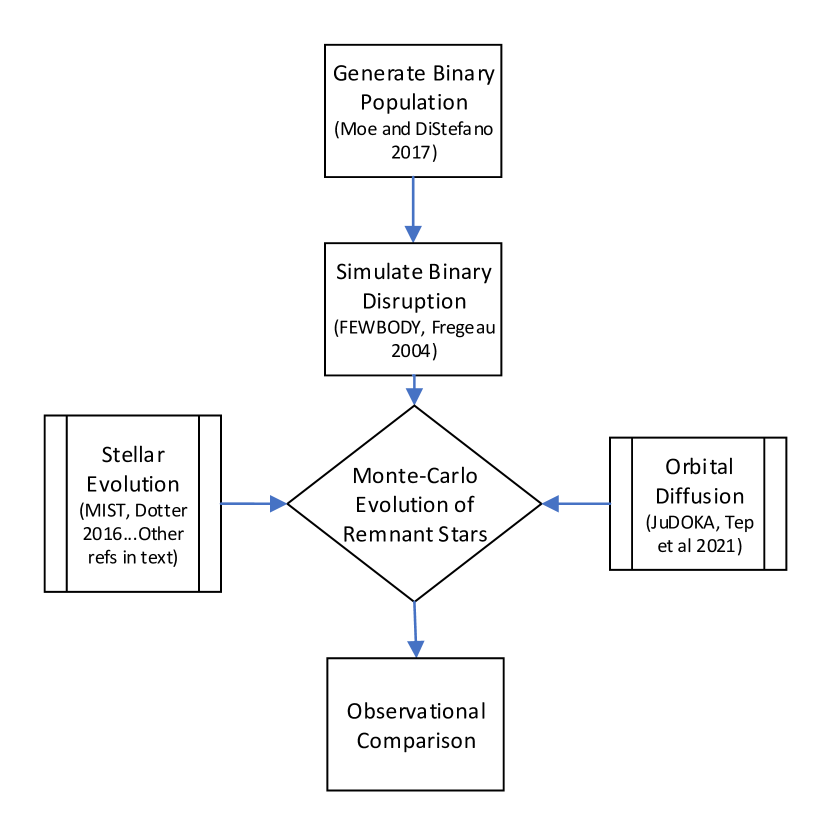
Figure 1: Flowchart summarizing the key steps in our model for the production of S-stars, including references and software used.

1. Generate model binaries following the assumptions in § 2.1.

   1. We only consider binaries with semi-major axes up to 15 au, as wider binaries are unlikely to deposit stars into the S-star region (see equation 3).

   2. The primary mass is between $1$ and $100M_{\odot}$. Lower mass binaries would not produce the presently-observed S-stars.

2. Generate close encounters with the SMBH following a Monte-Carlo procedure:

   1. The look-back time for the encounter is sampled uniformly between $10^{9}$ yr ago and the present day.

   2. The pericenter of the encounter is sampled uniformly between 16 gravitational radii ($\sim$ the tidal radius of a single star) and three times the maximum tidal radius of the binary population (equation 2). Thus, we implicitly assume binaries are in the full loss cone regime, such that the pericenter of the center-of-mass orbit is uniformly distributed. (See Merritt, 2013 for a discussion of loss cone physics).

   3. If the pericenter of the encounter exceeds three times the binary tidal radius (equation 2), the binary is unlikely to disrupt, and we proceed to the next one (Sari et al., 2010; Generozov & Madigan, 2020).

3. We simulate tidal encounters between each binary and the SMBH using the Fewbody code (Fregeau et al., 2004). In these encounters the binary is initialized at 50 tidal radii on a nearly parabolic with respect to the SMBH. The binary is generally split into low angular momentum bound and unbound stars (see § 2.1).

   1. We discard cases where the binary stars collide. This only happens $\sim 1\%$ of the time.

4. We collect all bound remnant stars with semi-major axes $<0.05$ pc, and follow their angular momentum and energy relaxation in a fixed background as described in § 2.2. The effect of the remnant stars on the background density profile is neglected (Fragione & Sari, 2018).

5. Stars are allowed to evolve and die (see § 2.3). Furthermore, stars may be tidally disrupted by the central SMBH (see equation 12)

6. We collect the properties of all surviving stars with semi-major axes $<0.05$ pc and K-band magnitudes $<18$, and compare to observations.

7. For each model star we compute the probability to measure its orbital elements according to equation 1 in Burkert et al. (2023). To account for observational bias, we exclude stars according to this probability.

3 Results

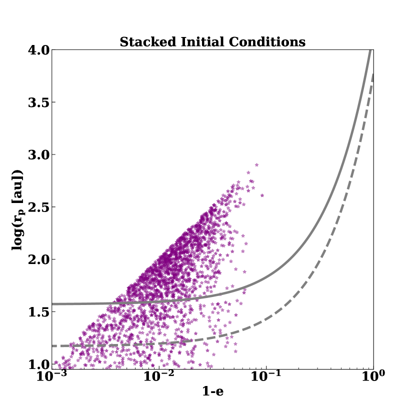
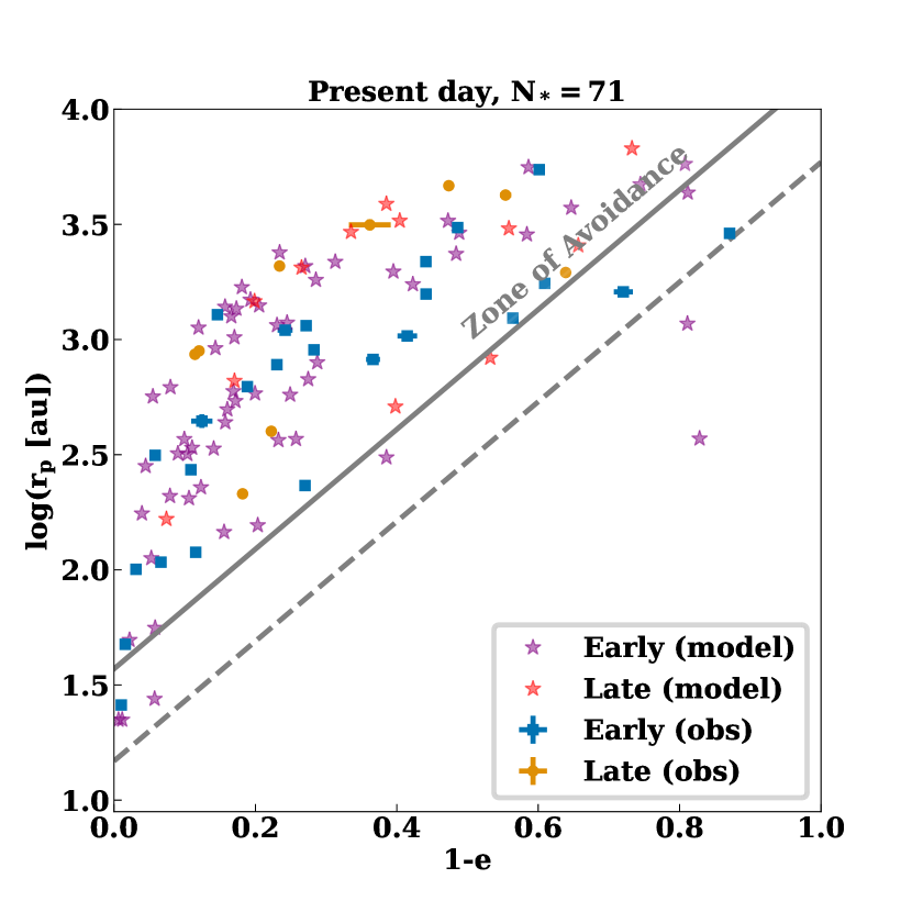
Figure 2: Initial (left) and final (right) pericenters and eccentricities for a subsample of model stars (Note the different x-scales in the two panels.) The left panel shows all stars, independently of when they are deposited in the Galactic Center. The right panel shows the 71 model stars surviving to the present day with $K\leq 18$ and $a\leq 0.05$ pc. Early (late) stars are shown in purple (red). Model stars initially have high eccentricities and evolve towards lower ones. For comparison, we show the observed S-stars with blue squares (early type) and orange (late type) circles in the right panel. The zone of avoidance from (Burkert et al., 2023) is shown as a solid, gray line. The dashed, gray line shows an adjusted zone of avoidance so that all S-stars are outside it.

The initial conditions of bound stars with semi-major axes, $a_{s}\leq 0.05$ pc are shown in the left panel of Figure 2. As expected, all stars start on highly eccentric orbits. The semi-major axis distribution is close to uniform, due to the approximately log-uniform semi-major axis distribution of the progenitor binaries, and our assumption of a full loss cone (see also Perets & Gualandris, 2010). The minimum semi-major axis is $\sim 5\times 10^{-4}$ pc, corresponding to remnants of near contact binaries (see equation 3). After $\sim 200$ Myr a quasi-steady state is reached in the S-star region. The final pericenter and eccentricity of surviving stars are shown in the right panel of Figure 2. Purple and red stars correspond to early and late-type stars, respectively. We also show the observed orbits of early and late-type S-stars with blue squares and orange circles, respectively. We group observed stars of unknown type with early stars. If they were late-type stars they would likely have been identified as such, considering CO absorption lines are prominent and therefore easily observed with current instruments. Unless otherwise specified, here and in other observational comparisons, we exclude (i) disc S-stars, (ii) Unbound S-stars, and (iii) S-stars with semi-major axes greater than 1.25”. Overall, we find reasonable agreement with the zone of avoidance. Approximately $\sim 14\%$ of model stars are in the zone of avoidance, as defined in Burkert et al. (2023). Similarly, in the latest orbital data, three of the $\sim 40$ observed stars are in the zone of avoidance (S14, S18, and S23). If we adjust the zone of avoidance so that all observed stars are outside (dashed gray line in Figure 2), then only $\sim 3.9\%$ of model stars are inside the modified zone. For 40 stars, this would correspond to a $\sim 20\%$ probability of no stars being in the zone of avoidance.

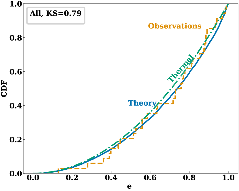
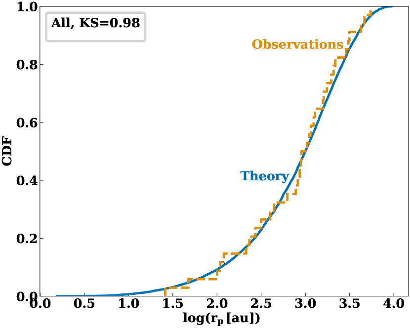
Figure 3: Top panel: Cumulative eccentricity distribution from the model (blue, solid), compared to the observed S-star eccentricity distribution (orange, dashed). For reference, we also show a thermal eccentricity distribution (green, dashed-dotted). Bottom panel: Cumulative pericenter distribution from our model and observations. The numbers in the legend are the p-values from a two-sample KS-test with the model and observed distributions.

Figure 3 shows the one-dimensional pericenter and eccentricity of our model stars, compared to the observed S-stars. Both distributions are consistent with the observations.

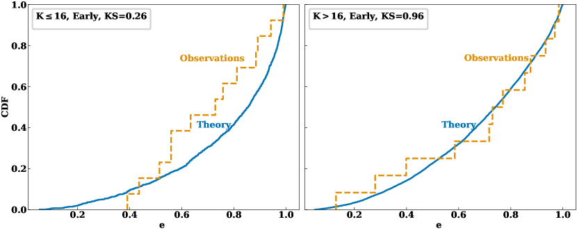
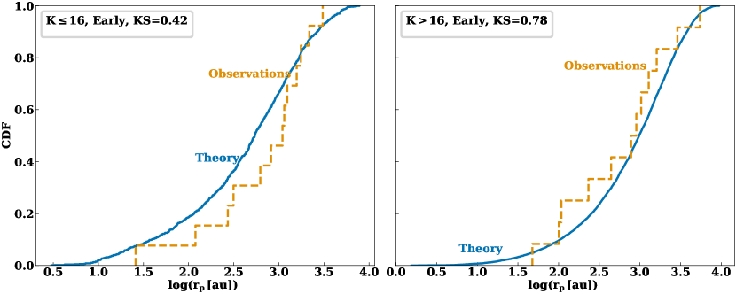
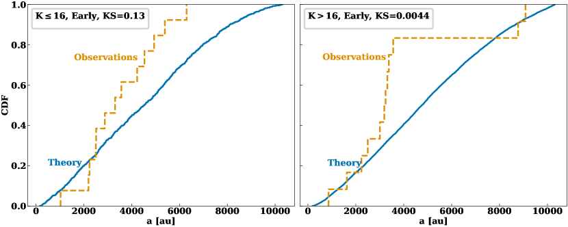
Figure 4: Cumulative eccentricity, pericenter, and semi-major axis distributions for bright ($K\leq 16$, left panels) and faint ($K>16$, right panels) early S-stars.

Figure 4 shows the orbital properties of early S-stars with $K\leq 16$ and $K>16$. Each group contains approximately the same number of stars. The eccentricity and pericenter distributions of each group are consistent with observations, though the bright stars have a somewhat superthermal eccentricity distribution. The faint stars’ semi-major axis distribution is too skewed towards large semi-major axes, compared to observations. In part, this is due to the assumed model for the progenitor binaries: as the primary mass decreases, the period distribution gradually shifts from approximately log-uniform to log-normal (with a peak near $10^{5}$ days). We also note that faint stars at large semi-major axes are the most difficult to detect, and this comparison is subject to observational bias.

We now compare the stellar properties of model stars with observations. In the model, $\sim 20\%$ of stars are late-type. This is consistent (within Poisson uncertainties) with the observed fraction $\sim 26\%$. However, we note that we have not included disruptions of old ($\mathrel{\hbox to0.0pt{\lower 4.0pt\hbox{\hskip 1.0pt$\sim$}\hss}\raise 1.0pt\hbox{$>$}}10^{10}$) stars that make up the bulk of the nuclear stellar disc, and that can increase the population of evolved stars in the S-star region.

We also compare the K-band magnitudes of our model stars to observations (Figure 5). In practice, we use the JWST F210M magnitude from MIST isochrones (Dotter, 2016; Choi et al., 2016; Paxton et al., 2011, 2013, 2015), to approximate the K-band magnitude of our model stars. We also assume an extinction of 2.42 (Fritz et al., 2011) and a galactocentric distance of 8.3 kpc (GRAVITY Collaboration et al., 2021). We neglect corrections from differential extinction ($\sim 0.3$ mag; Schödel et al., 2010; Do et al., 2013).

The bottom panel of Figure 5 compares the overall K-band luminosity functions (KLF) from theory and observations. We rescale the luminosity functions to match at $K=16.2$. There are significant discrepancies between the model and observed S-star K-band luminosity function at both the faint and bright ends. The former can plausibly be explained by completeness effects. The latter is due to $\sim 3$ bright giants with $K<14$ that are not observed, and is of marginal significance. We note that collisions with black holes cannot remove these bright giants (see § 4.2).

The top panel of Figure 5 compares the model and observed KLF of early-type stars (blue and orange). Here, there are no large differences at the bright end, while the model has many more stars with $K>16$. This discrepancy may again be due to completeness effects. Unfortunately this is difficult to quantify, as the observational selection function is highly non-trivial (the orange KLF only includes stars with measured orbits). The model more closely matches overall KLF from Schödel et al. (2020) (light red points; see Appendix B for details), which should be more complete, as even stars without orbits are included.

However, the progenitor binaries are more likely to follow a present-day mass function rather than an initial mass function (as assumed here). A present-day mass function would steepen the model KLF, and exacerbate the tension with observations (see § 4).

The top panel of Figure 6 shows the K-band magnitude as a function of age for the eight bright ($K\leq 15.5$) S-stars from Habibi et al. (2017) and for our model stars, which appear significantly older. To better compare the age distributions, we select a subset of model stars with comparable K magnitudes. First, we select all model stars within 0.1 mag for each of the Habibi et al. (2017) stars. Then, we sample 100 stars (with replacement) from each of these subsets. The gray line in the bottom panel of Figure 6 shows the stacked age distribution of the selected stars. On average, model stars are significantly older, even after accounting for the observational bias towards bright stars. This may suggest that the brightest S-stars have a distinct origin or that the star formation rate (and delay time distribution between star formation and disruption) is non-uniform. Finally, there is a degeneracy between the age and metallicity (see Appendix C), such that the S-stars may in fact have sub-solar metallicity and be significantly older. Currently there are no measurements of metallicity for the S-stars, but future observations of the S-stars with ERIS and NIRSpec will constrain this. A priori, this explanation is less likely, considering the nuclear stellar disc and nuclear star cluster are mostly metal rich with small metal-poor populations (Do et al., 2015; Feldmeier-Krause et al., 2017; Rich et al., 2017; Nandakumar et al., 2018; Schultheis et al., 2019; Schödel et al., 2020; Schultheis et al., 2021; Nieuwmunster et al., 2024; Nogueras-Lara et al., 2024).

Finally, Figure 7 shows a corner plot of $a$, $e$, and $K$. Once again, we see good agreement between the observed and theoretical eccentricity distributions. At the same time, the model produces too many faints stars, and too many stars at large semi-major axes (though again we caution that faint stars at large semi-major axes are the most difficult to detect, and the latter discrepancy may be due to observational bias). In the observations, many of the lowest eccentricity stars are in a narrow band of semi-major axes ($3.3\mathrel{\hbox to0.0pt{\lower 4.0pt\hbox{\hskip 1.0pt$\sim$}\hss}\raise 1.0pt\hbox{$<$}}\log(a/{\rm au})\mathrel{\hbox to0.0pt{\lower 4.0pt\hbox{\hskip 1.0pt$\sim$}\hss}\raise 1.0pt\hbox{$<$}}3.55$). This feature is not apparent in the model. However, there are not enough stars to conclude this is a statistically significant difference. Furthermore, the absence of this feature may simply reflect the differences in the one-dimensional semi-major axis distributions. To test this, we select the model star with the closest semi-major axis for each observed S-star. The structure of these model stars in $a-e$ space is more similar to the observed one, as shown in the bottom panel of Figure 7. Interestingly, there is a band of low eccentricity stars near the galactocentric radius where the scalar resonant relaxation time is minimized ($\log(a/{\rm au})\approx 3.24$). This is where angular momentum relaxation is most efficient.

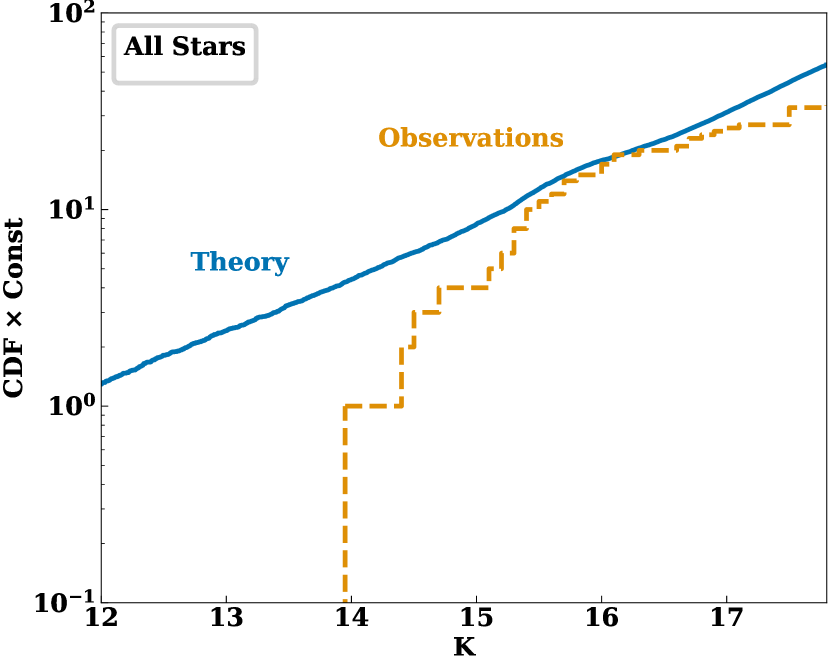
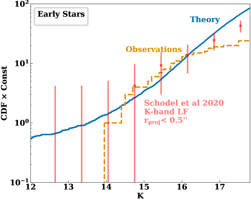
Figure 5: Top panel: K-band luminosity function of all model (blue) and observed (orange, dashed) S-stars. Bottom panel: K-band luminosity functions for model (blue) and observed (orange, dashed) early S-stars (with orbits). The red line is the K-band luminosity function of early stars in the central 0.5” from Schödel et al. (2020) (red line; see Appendix B for details). The luminosity functions are normalized to match at a K-band magnitude of 16.2.

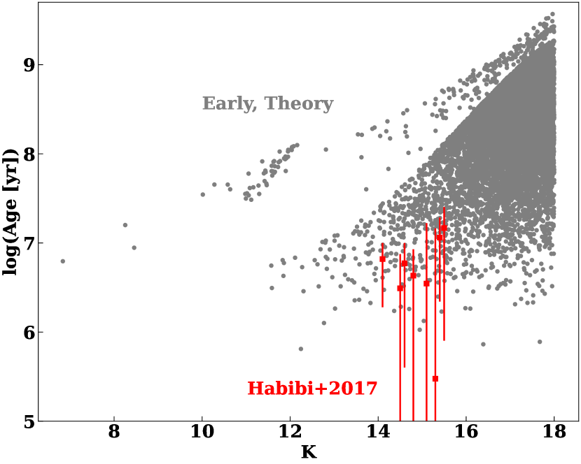
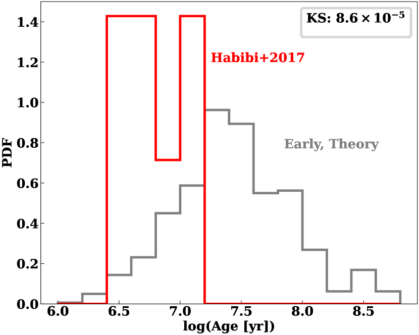
Figure 6: Top panel: Age versus K-band magnitude for eight bright S-stars (red; Habibi et al., 2017), compared to early model stars (gray). Bottom: Age distribution of Habibi et al. (2017) stars and model stars with comparable magnitudes (see text for details).

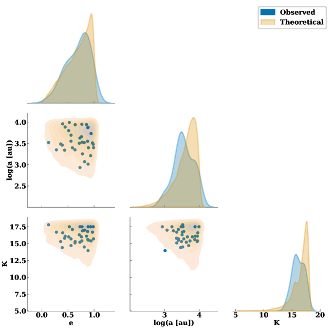
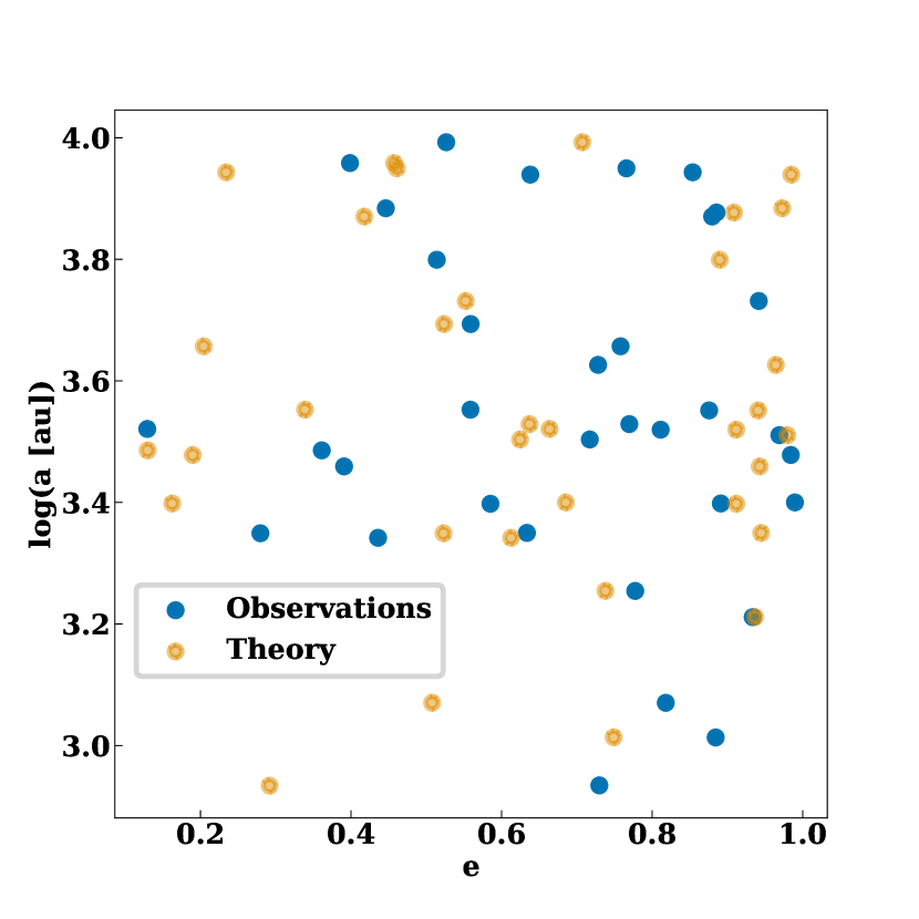
Figure 7: Top panel: Corner plot showing distributions of semi-major axis ($a$), eccentricity ($e$), and $K$ magnitude from theory (orange) and observations (blue). Bottom panel: Eccentricity versus semi-major axis for the observed S-stars, and for the model stars that are closest in semi-major axis.

4 Critical discussion of model assumptions

Here we critically examine two assumptions about the progenitor binary population, and how they affect observational comparisons. Firstly, the primary mass of each binary is drawn from an initial mass function. However, a steeper present-day mass function is more realistic, considering the shorter lifetimes of massive stars. Secondly, binaries are allowed to disrupt immediately after formation. In reality, binaries may need some time to reach disruption, especially if they form on circular orbits. As discussed below, delays and a present-day mass function exacerbate the tension with the observed K-band luminosity function.

We also discuss the effect of stellar collisions and repeated, individually non-disruptive tidal encounters between the stars and the central SMBH. These effects are not included in our base model, but do not affect the results.

4.1 Mass function and disruption times

In our base model, the primary mass of each binary is drawn from a Kroupa initial mass function. However, the mass function of disrupting binaries will likely be more bottom-heavy, due to the longer lifetimes of low-mass stars.

Here we account for this effect by re-weighting probability distributions. In particular, each remnant star is weighted by the main sequence lifetime of the primary star in the progenitor binary. This causes the K-band luminosity function to steepen, in tension with observations, as shown in Figure 8.

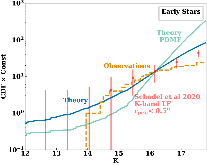
Figure 8: The light green line shows the luminosity function, accounting for the dependence of the binary disruption probability on stellar lifetime. (Effectively, the progenitor binaries are drawn from a present-day mass function rather than an initial mass function). The other lines are the same as in Figure 5.

This result depends on the star formation history in the Galactic Center, particularly within the region of the nuclear stellar disc, where disrupting binaries likely originate. Schödel et al. (2023) recently showed that the star formation history in the nuclear stellar disc is highly non-uniform: $\mathrel{\hbox to0.0pt{\lower 4.0pt\hbox{\hskip 1.0pt$\sim$}\hss}\raise 1.0pt\hbox{$>$}}70\%$ of the stars formed more than $10$ Gyr ago, $\sim 15\%$ formed $\sim 1$ Gyr ago and up to $10\%$ formed in the last tens to hundreds of Myr. This suggests a star formation rate rising towards the present-day (since a comparable of stars were formed within the last $\sim 10^{8}$ yr and $\sim 10^{9}$ yr). Furthermore, the star formation rate is likely correlated with the binary disruption rate, since both are correlated to the molecular gas density.

Motivated by these observations, we discard stars that formed more than $10^{8}$ yr ago. Figure 9, shows the K-band luminosity function after this cut, with and without re-weighting for stellar lifetimes. In the former case, massive stars receive a weight equal to their main sequence lifetime divided by $10^{8}$ yr. Stars with main sequence lifetimes longer than $10^{8}$ yr receive a weight of unity. This ameliorates, but does not entirely remove the tension with observations, as shown in Figure 9. Furthermore, the model eccentricity distribution is in tension with observations, though this can be resolved if the background black holes are each 20 $M_{\odot}$ instead of 10 $M_{\odot}$.

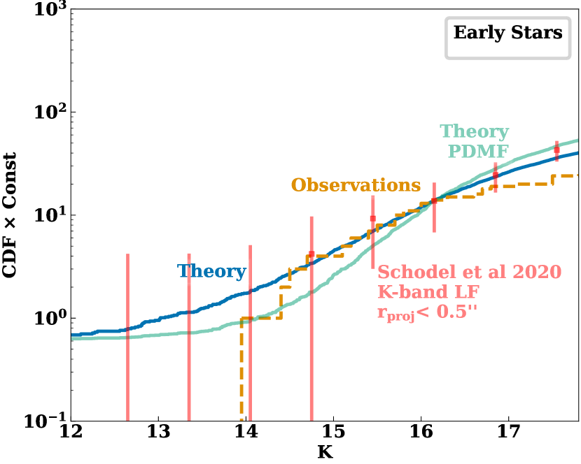
Figure 9: K-band luminosity functions, after discarding stars formed more than $10^{8}$ yr ago. The blue (light green) line corresponds to binaries drawn from an initial (present-day) mass function.

The results also depend on the delay time distribution between star formation and disruptions. In the base model, binaries can be disrupted immediately after formation. More realistically, binaries will take some time to reach the loss cone, especially if they form on circular orbits. Imposing a minimum age at disruption tends to steepen the K-band luminosity function, as illustrated in Figure 10. This shows the K-band luminosity function after (i) Discarding stars older $10^{8}$ yr and (ii) Discarding stars that disrupted less than $10^{7}$ yr after formation.

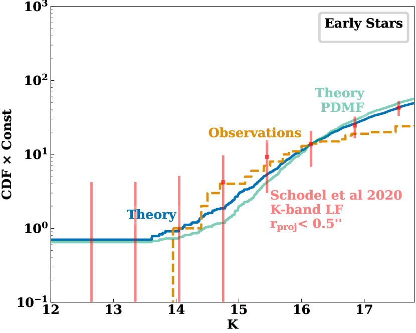
Figure 10: Same as Figure 9, except we discard stars that were less that $10^{7}$ yr old at the moment of disruption.

The better agreement between theory and observation in Figure 9 suggests that the early S-stars are primarily sourced by binaries formed within the last $\sim 100$ Myr. Nonetheless a slight tension remains, especially for realistic delay times between star formation and disruption, as in Figure 10. In this case, there is a $\sim$2$\sigma$ tension between the observed (orange) and theoretical (turquoise) KLF between $K=14$ and $K=16$. Potentially, this tension could be resolved via a bursty star formation rate that is more skewed towards the present day.

Alternatively, the tension with the observed KLF may be resolved with a top-heavy initial mass function. The mass function required itself depends on the binary injection history. In the last case (Figure 10), an initial mass function of $dN/dm\propto m^{-0.2}$ reduces the tension to 1$\sigma$.

4.2 Collisions

In principle, stars may suffer mass loss or destruction via collisions with other stars or compact objects. Alternatively, star-star collisions can lead to mergers and the build-up of massive stars (Spitzer & Saslaw, 1966; Duncan & Shapiro, 1983; Murphy et al., 1991; Genzel et al., 1996; Davies et al., 1998; Portegies Zwart et al., 1999; Gürkan et al., 2004; Freitag et al., 2006b; Dale et al., 2009; Rose et al., 2023).

Here, we estimate the impact of destructive black-hole star collisions. In particular, we compute the orbit-averaged collision rate between the remnant stars and black holes in our Monte-Carlo models, viz.

$$\Gamma_{\rm coll}(r)=n_{\rm bh}(r)v(r)r_{*}^{2}\left(1+2\frac{G(m_{\rm bh}+m_{*})}{v(r)^{2}r_{*}}\right),$$ (13)

where $m_{*}$ and $m_{\rm bh}$ are the stellar and BH masses respectively, $r_{*}$ is the stellar radius, $v(r)\approx\sqrt{GM_{\rm bh}/r}$, is the local velocity dispersion, and $n_{\rm bh}(r)$ is the BH density (see eq 7). The orbit average is calculated from $10^{4}$ points along the orbit, equally spaced in eccentricity anomaly ($EA$). Each point is weighted by $\left(1-e\cos(EA)\right)$ in the average.

For each Monte-Carlo timestep, $\delta t$, we generate a random number between 0 and 1, and record a collision if it is less than the expected number of collisions, $<\Gamma_{\rm coll}>\delta t$.

Removing stars that experience collisions has a minor impact on the results. Most notably, the fraction of late-type S-stars decreases from $\sim 20\%$ to $\sim 16\%$. In fact, the impact of collisions may be overestimated, considering deeply penetrating encounters are necessary to significantly dim giant stars (Dale et al., 2009).

Rose et al. (2023) showed that star-star collisions in the S-star region can lead to the build-up of massive stars (but this would require non-disruptive collisions). We leave this effect to future studies, though it may have a major impact on the comparisons to the observed K-band luminosity function and ages. Additionally, stellar collisions can lead to TDE-like or SNe-like transients (Balberg et al., 2013; Amaro Seoane, 2023; Ryu et al., 2024; Dessart et al., 2024).

4.3 Repeated tidal encounters with the SMBH

So far, we have only considered the removal of stars due to full tidal disruptions by the central SMBH. However, stars may also be removed due to multiple partial tidal disruptions. Furthermore, stars may become swollen and disrupted due to tidal heating (Alexander & Morris, 2003).

To experience such effects the star needs to pass within a factor of a few of the central SMBH (Guillochon & Ramirez-Ruiz, 2013; Li & Loeb, 2013; Mainetti et al., 2017; Ryu et al., 2020b; Lu et al., 2021; Generozov, 2021).

To test how these effects would change the results, we multiply the tidal radius of each star by two. We find that this has no significant effect on the comparisons previously discussed.

5 Fixed age model (Eccentric disc)

So far, we have considered models, where stellar ages and disruption times can vary freely. We now discuss models, where all stars are injected at similar times in the recent past. Such an impulsive burst of disruptions may be triggered by a secular gravitational instability in the $\sim 2.5-8$ Myr old (Levin & Beloborodov, 2003; Paumard et al., 2006; Bartko et al., 2009; Lu et al., 2013; Yelda et al., 2014) clockwise disc if it starts in a lopsided, eccentric configuration (Madigan et al., 2009; Generozov & Madigan, 2020; Rantala & Naab, 2023). This configuration can arise from the tidal disruption of a molecular cloud (Bonnell & Rice, 2008; Gualandris et al., 2012; Generozov et al., 2022), or via an SMBH merger in the Galactic Center (Akiba et al., 2024). Interactions between the misaligned young disks may also trigger a burst of binary disruptions (Löckmann et al., 2008).

Previously, Generozov & Madigan (2020) and Tep et al. (2021) analyzed the relaxation of the S-stars in such scenarios. The former found that $10M_{\odot}$ BHs would be able to reproduce the observed S-star eccentricity distribution, by modeling angular momentum relaxation at a fixed semi-major axis of 0.01 pc. However, the resonant relaxation time will be significantly longer in the outer part of the S-star cluster. Tep et al. (2021) accounted for the S-stars’ semi-major axis distribution, and found that reproducing the observed S-star eccentricity distribution requires black holes above $100M_{\odot}$ at $2\sigma$ confidence, though this constraint depends on the S-star sample (i.e. this is the constraint including late-type and disc S-stars).

We perform a similar analysis, assuming stars are injected into the Galactic Center all at once. First, for consistency with Tep et al. (2021), we turn off (i) the loss cone, (ii) stellar evolution, and (iii) semi-major axis diffusion. Effects (i) and (ii) will be negligible for the S-stars over Myr timescales. However, we show that the loss cone can affect black hole mass constraints at the factor of $\sim 2$ level.

We also match the initial conditions in Tep et al. (2021), assuming all stars were injected into the Galactic Center 7.1 Myr ago, the mean age of eight bright S-Stars from Habibi et al. (2017). The initial angular momentum distribution is a Gaussian with a mean of 0.2 ($e=0.98$) and a standard deviation of 0.02.

We present results for both the density profiles in Tep et al. (2021), viz.

$$\rho_{\rm bh}=3.6\times 10^{6}\left(\frac{r}{0.1\,{\rm pc}}\right)^{-1.8}M_{\odot}\,{\rm pc}^{-3}$$

$$\rho_{\rm*}=9.4\times 10^{5}\left(\frac{r}{0.1\,{\rm pc}}\right)^{-1.5}M_{\odot}\,{\rm pc}^{-3},$$ (14)

and our fiducial density profile (eq 7) that is in better agreement with the latest constraints from GRAVITY (Collaboration et al., 2024) and has a factor of $3$ fewer BHs within 0.05 pc.

Using the same S-star sample and background profile as Tep et al. (2021), we find good agreement with their results: black hole masses $<100M_{\odot}$ can be ruled out. However, the full sample includes late-type stars and stars at larger scales that may be unrelated to binary disruptions. For example, eight of the S-stars are members of the clockwise disc. For the 25 early, non-disc S-stars with semi-major axes within 0.05 pc, only black holes with masses $<17M_{\odot}$ can be ruled out. For the same subsample and our fiducial density profile, masses $<50M_{\odot}$ can be ruled out. Finally, the lower limit is reduced to $\sim 24M_{\odot}$, with a loss cone.

Overall, explaining the entire S-star population via binaries from the young clockwise disc requires a background with more massive black holes. There is also tension between the mass functions of the disc and S-stars that may require an unusual mass ratio distribution within the disc to reconcile (Generozov, 2021). Moreover, it is not clear whether the conditions for the eccentric disc instability could arise with steep background density profiles (e.g. eq 7; see the discussions in Madigan et al., 2009 and Generozov et al., 2022). On the other hand, efficient angular momentum relaxation of the S-stars likely requires a steep black hole cusp.

Detailed modeling of disc binary disruptions suggests that they can reproduce the zone of avoidance, but remnant stars will be skewed towards large semi-major axes compared to the observations.

6 Summary and Discussion

We show that many properties of the observed S-star cluster in the Galactic Center, including the recently discovered zone of avoidance, can be explained by a combination of isotropic binary disruptions, and relaxation in the Galactic Center. Our focus is on explaining the classic, isotropic S-star cluster. In our model, the young discs would have a different origin that we leave to future work.

Our main conclusions are summarized as follows.

1. In the full-loss-cone regime the remnant stars from massive binary disruptions will have an approximately uniform semi-major axis distribution. This naturally explains the lack of S-stars in the zone of avoidance. Empty loss cone models would place too many stars in this region.

2. The overall orbital eccentricity and pericenter distribution of the S-star cluster is well reproduced in our models, via relaxation processes. We only consider non-resonant and resonant relaxation from a background population of stars and $10M_{\odot}$ black holes. Potentially, an AGN disc may also perturb the S-star orbits, dramatically reducing the angular momentum relaxation time (Chen & Amaro-Seoane, 2014).

3. There is a slight tension with the observed semi-major axis distribution of fainter S-star ($K<16$), potentially indicating the progenitor binary population is more skewed to small separations than in Moe & Di Stefano (2017).

4. The model K-band luminosity function is in tension with observations, particularly with a Kroupa present-day mass function and realistic delay times between star formation and disruption. Potentially, this tension may be resolved with a top-heavy initial mass function or with a bursty star formation rate that is skewed towards the present day. However, reproducing the observed thermal eccentricity distribution would be more challenging in such scenarios.

5. There is also tension with the measured ages of the bright S-stars, with the model predicting older ages. Again, this may point to a bursty star formation rate. Alternatively, the measured ages may be underestimated if the S-stars have sub-solar metallicities.

Appendix A Binary Evaporation

In principle, the binary population in the Galactic Center region may be shaped by dynamical processes. For example, soft binaries can be evaporated by encounters with other stars. Here we quantify this effect and show that in our models binaries are more likely to disrupt rather than evaporate, and thus binary evaporation may be neglected.

The local evaporation timescale is (cf Alexander & Pfuhl, 2014)

$$t_{\rm evap} =0.07\frac{v_{12}^{2}\sigma}{G^{2}n<m^{2}>\ln\Lambda_{12}}$$

$$=2.6\times 10^{10}{\rm yr}\left(\frac{a_{\rm bin}}{15{\rm au}}\right)^{-1}\left(\frac{<m^{2}>}{1M_{\odot}}\right)^{-1}\left(\frac{m_{\rm bin}}{6M_{\odot}}\right)$$

$$\left(\frac{\sigma}{100{\rm kms^{-1}}}\right)\left(\frac{n}{5000{\rm pc^{-3}}}\right)\ln\Lambda_{12}^{-1},$$ (15)

where $v_{12}$ is the internal velocity of the binary, $n$, $\sigma$, and $<m^{2}>$ are the number density, velocity dispersion of the perturbing population, and $\Lambda_{12}=2\sigma^{2}/v_{12}^{2}$. In our model, binaries come from outside the central 5 pc, where $n\approx 5\times 10^{3}$ pc^-3, and $\sigma\approx 100$ km s^-1. For binaries with semi-major axes $\leq 15$ au in this region the evaporation timescale is of order 10 Gyr or more.

In comparison, the timescale for binaries to disrupt is

$$t_{\rm dis}=\frac{r}{\sigma}\frac{j_{c}^{2}}{j_{\rm lc}^{2}},$$ (16)

where $j_{lc}=\sqrt{2GM_{\rm bh}r_{t}}$. For an enclosed mass of $10^{7}M_{\odot}$ inside 5 pc,

$$t_{\rm dis}(5{\rm pc})\approx 3\times 10^{7}{\rm yr}\left(\frac{\sigma}{100{\rm kms^{-1}}}\right)^{-1}\left(\frac{m_{\rm bin}}{6M_{\odot}}\right)^{-1/3}\left(\frac{a_{\rm bin}}{15{\rm au}}\right)^{-1}$$ (17)

Binaries on eccentric orbits will cross the central region where the evaporation timescale is shorter. In particular the evaporation timescale will be between $r^{1.3}-r^{1.5}$. The average evaporation time over the binary population is

$$<t_{\rm evap}>=\int_{0}^{e_{\rm max}}def(e)\left(\int_{r_{p}}^{r_{a}}dr\frac{2}{Pt_{\rm evap}}\frac{1}{v_{r}}\right)^{-1},$$ (18)

where $r_{p}$, $r_{a}$, $v_{r}$, $P$, $e$, and $f(e)$ are the pericenter, apocenter, radial velocity, orbital period, eccentricity, and eccentricity distribution respectively. Note that the inner integral corresponds to a harmonic average.

In steady state $f(e)$ is expected to be thermal. Also, since we are considering binaries that are not too far outside the SMBH sphere of influence, we assume Keplerian scalings with radius for all the dynamical quantities. Overall, we find eccentric orbits give a $\sim 10\%$ correction to the evaporation time.

Although we have focused on soft binaries, the hardening rate of hard binaries has a similar dependence on cluster and binary properties (Heggie, 1975; Hills, 1983). Therefore, we also expect hard binaries to disrupt before they can significantly harden.

Appendix B K-band luminosity function

Here we describe how we derive the KLF of early stars inside of 0.5” (the red line in Figure 5) from the data in Schödel et al. (2020).

First we compute the KLF in two radial rings with $r_{\rm proj}<0.5\arcsec$ and $4\arcsec<r_{\rm proj}<5\arcsec$. These KLFs include contribution from both early and late stars, with surface density profiles $r^{-0.8\pm 0.08}$ and $r^{0\pm 0.08}$, respectively (Table 6 in Gallego-Cano et al., 2024). The surface densities are equal at $\sim 0.7\arcsec$, such that late (early) stars dominate on larger (smaller) scales.

The KLF of early stars within $0.5\arcsec$ is

$$K_{\rm early,0.5}\approx K_{0.5}-WK_{4}$$ (19)

where $K_{0.5}$ is the total KLF inside of $0.5\arcsec$ and $K_{4}$ is the KLF between $4\arcsec$ and $5\arcsec$, which is dominated by late stars. The weight, W, is chosen to reproduce the ratio of late to all stars inside of $0.5\arcsec$, $X$. From the surface density profiles in Gallego-Cano et al. (2024), $X\approx 0.3$ and

$$W=\frac{N(r_{\rm proj}<0.5\arcsec,K\leq 16.15)}{N(4\arcsec<r_{\rm proj}<5\arcsec,K\leq 16.15)}X\approx 1.3,$$ (20)

where the numerator is the number of stars with projected radius, $r_{\rm proj}$ less than $0.5\arcsec$ and $K\leq 16$. Similarly, the denominator is the number of stars with $4\arcsec<r_{\rm proj}<5\arcsec$ and $K\leq 16.15$. The cut near $K=16.15$ is motivated by exclusion of fainter stars from the surface density fits in Gallego-Cano et al. (2024).

From equations (19) and (20), we obtain the $K_{\rm early,0.5}$, the red line in Figure 5. The uncertainty is calculated by adding the uncertainties from $K_{0.5}$ and $K_{4}$ in quadrature. The results change by less than the uncertainty, if we use the KLF from $2$–$3\arcsec$ or $3$–$4\arcsec$ in lieu of $K_{4}$. In fact, the difference between $K_{0.5}$ and $K_{\rm early,0.5}$ are smaller than the uncertainties for $K\lesssim 19$.

Appendix C S-star Ages versus Metallicity

Here we show that the S-star ages are degenerate with metallicity. Figure 11 shows a comparison of MIST isochrones of $\log(g)$ versus $\log(T_{\rm eff})$ for two different metallicities. Qualitatively, the S-stars can either be younger and metal rich or older and metal poor. For each star, we estimate the age by identifying the closest main sequence isochrone point. We summarize these estimates in Table 1, along with the fits from Habibi et al. (2017). We emphasize that our ages are merely estimates to illustrate the trend with metallicity, rather than detailed fits.

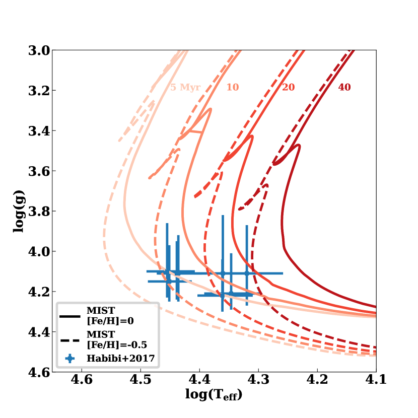
Figure 11: $\log(g)$ versus $\log(T_{\rm eff})$ for the eight bright S-stars from Habibi et al. (2017) compared to MIST isochrones (v1.2, $v/v_{\rm crit}=0.4$). The solid (dashed) lines correspond to $[{\rm Fe/H}]=0$ ($[{\rm Fe/H}]=-0.5$).

Table 1: Ages for eight bright S-stars from Habibi et al. (2017), and from MIST isochrones at different metallicities.

Star	Habibi et al 2017	MIST, [Fe/H]=0.0	MIST, [Fe/H]=-0.5	MIST, [Fe/H]=-1.0
	[Myr]	[Myr]	[Myr]	[Myr]
S1	${4.3}_{-4.2}^{+4.2}$	5.0	10.0	14.1
S2	${6.6}_{-4.7}^{+3.4}$	4.5	7.9	11.2
S4	${5.9}_{-5.5}^{+4.1}$	5.0	10.0	14.1
S6	${11.5}_{-9.3}^{+7.8}$	8.9	17.8	25.1
S7	${0.3}_{-0.3}^{+14.3}$	4.0	15.8	25.1
S8	${3.1}_{-3.0}^{+4.4}$	3.2	7.9	11.2
S9	${3.5}_{-3.5}^{+13.2}$	5.0	15.8	25.1
S12	${14.7}_{-13.9}^{+10.6}$	14.1	28.2	35.5

References

- Aharon & Perets (2015) Aharon, D. & Perets, H. B. 2015, ApJ, 799, 185
- Akiba et al. (2024) Akiba, T., Naoz, S., & Madigan, A.-M. 2024, arXiv e-prints, arXiv:2410.19881
- Alexander (2017) Alexander, T. 2017, ArXiv e-prints [arXiv:1701.04762]
- Alexander & Hopman (2009) Alexander, T. & Hopman, C. 2009, ApJ, 697, 1861
- Alexander & Morris (2003) Alexander, T. & Morris, M. 2003, ApJ, 590, L25
- Alexander & Pfuhl (2014) Alexander, T. & Pfuhl, O. 2014, ApJ, 780, 148
- Amaro Seoane (2023) Amaro Seoane, P. 2023, ApJ, 947, 8
- Antonini et al. (2010) Antonini, F., Faber, J., Gualandris, A., & Merritt, D. 2010, ApJ, 713, 90
- Antonini & Merritt (2013) Antonini, F. & Merritt, D. 2013, ApJ, 763, L10
- Astropy Collaboration et al. (2022) Astropy Collaboration, Price-Whelan, A. M., Lim, P. L., et al. 2022, ApJ, 935, 167
- Astropy Collaboration et al. (2013) Astropy Collaboration, Robitaille, T. P., Tollerud, E. J., et al. 2013, A&A, 558, A33
- Bahcall & Wolf (1976) Bahcall, J. N. & Wolf, R. A. 1976, ApJ, 209, 214
- Balberg et al. (2013) Balberg, S., Sari, R., & Loeb, A. 2013, MNRAS, 434, L26
- Bar-Or & Alexander (2014) Bar-Or, B. & Alexander, T. 2014, Classical and Quantum Gravity, 31, 244003
- Bar-Or & Alexander (2016) Bar-Or, B. & Alexander, T. 2016, ApJ, 820, 129
- Bar-Or & Fouvry (2018) Bar-Or, B. & Fouvry, J.-B. 2018, ApJ, 860, L23
- Bartko et al. (2009) Bartko, H., Martins, F., Fritz, T. K., et al. 2009, ApJ, 697, 1741
- Baumgardt et al. (2018) Baumgardt, H., Amaro-Seoane, P., & Schödel, R. 2018, A&A, 609, A28
- Bonnell & Rice (2008) Bonnell, I. A. & Rice, W. K. M. 2008, Science, 321, 1060
- Bradnick et al. (2017) Bradnick, B., Mandel, I., & Levin, Y. 2017, MNRAS, 469, 2042
- Bressan et al. (2012) Bressan, A., Marigo, P., Girardi, L., et al. 2012, MNRAS, 427, 127
- Burkert et al. (2023) Burkert, A., Gillessen, S., Lin, D. N. C., et al. 2023, arXiv e-prints, arXiv:2306.02076
- Cao et al. (2024) Cao, C. Y., Liu, F. K., Li, S., Chen, X., & Wang, K. 2024, arXiv e-prints, arXiv:2411.09278
- Chen & Amaro-Seoane (2014) Chen, X. & Amaro-Seoane, P. 2014, ApJ, 786, L14
- Chen et al. (2015) Chen, Y., Bressan, A., Girardi, L., et al. 2015, Monthly Notices of the Royal Astronomical Society, 452, 1068
- Chen et al. (2014) Chen, Y., Girardi, L., Bressan, A., et al. 2014, Monthly Notices of the Royal Astronomical Society, 444, 2525
- Choi et al. (2016) Choi, J., Dotter, A., Conroy, C., et al. 2016, ApJ, 823, 102
- Collaboration et al. (2024) Collaboration, T. G., Dayem, K. A. E., Abuter, R., et al. 2024, Improving constraints on the extended mass distribution in the Galactic Center with stellar orbits
- Dale et al. (2009) Dale, J. E., Davies, M. B., Church, R. P., & Freitag, M. 2009, MNRAS, 393, 1016
- Davies et al. (1998) Davies, M. B., Blackwell, R., Bailey, V. C., & Sigurdsson, S. 1998, MNRAS, 301, 745
- Dessart et al. (2024) Dessart, L., Ryu, T., Amaro Seoane, P., & Taylor, A. M. 2024, A&A, 682, A58
- Do et al. (2019) Do, T., Hees, A., Ghez, A., et al. 2019, Science, 365, 664
- Do et al. (2015) Do, T., Kerzendorf, W., Winsor, N., et al. 2015, ApJ, 809, 143
- Do et al. (2013) Do, T., Lu, J. R., Ghez, A. M., et al. 2013, ApJ, 764, 154
- Dotter (2016) Dotter, A. 2016, ApJS, 222, 8
- Duncan & Shapiro (1983) Duncan, M. J. & Shapiro, S. L. 1983, ApJ, 268, 565
- Feldmeier-Krause et al. (2017) Feldmeier-Krause, A., Kerzendorf, W., Neumayer, N., et al. 2017, MNRAS, 464, 194
- Fouvry et al. (2017) Fouvry, J. B., Pichon, C., & Magorrian, J. 2017, A&A, 598, A71
- Fragione et al. (2017) Fragione, G., Capuzzo-Dolcetta, R., & Kroupa, P. 2017, MNRAS, 467, 451
- Fragione & Sari (2018) Fragione, G. & Sari, R. 2018, ApJ, 852, 51
- Fregeau et al. (2004) Fregeau, J. M., Cheung, P., Portegies Zwart, S. F., & Rasio, F. A. 2004, MNRAS, 352, 1
- Freitag et al. (2006a) Freitag, M., Amaro-Seoane, P., & Kalogera, V. 2006a, ApJ, 649, 91
- Freitag et al. (2006b) Freitag, M., Gürkan, M. A., & Rasio, F. A. 2006b, MNRAS, 368, 141
- Fritz et al. (2011) Fritz, T. K., Gillessen, S., Dodds-Eden, K., et al. 2011, ApJ, 737, 73
- Gallego-Cano et al. (2024) Gallego-Cano, E., Fritz, T., Schödel, R., et al. 2024, A&A, 689, A190
- Gallego-Cano et al. (2018) Gallego-Cano, E., Schödel, R., Dong, H., et al. 2018, A&A, 609, A26
- Generozov (2021) Generozov, A. 2021, MNRAS, 501, 3088
- Generozov & Madigan (2020) Generozov, A. & Madigan, A.-M. 2020, ApJ, 896, 137
- Generozov et al. (2022) Generozov, A., Nayakshin, S., & Madigan, A. M. 2022, MNRAS, 512, 4100
- Generozov et al. (2018) Generozov, A., Stone, N. C., Metzger, B. D., & Ostriker, J. P. 2018, MNRAS, 478, 4030
- Genzel et al. (1997) Genzel, R., Eckart, A., Ott, T., & Eisenhauer, F. 1997, MNRAS, 291, 219
- Genzel et al. (1996) Genzel, R., Thatte, N., Krabbe, A., Kroker, H., & Tacconi-Garman, L. E. 1996, ApJ, 472, 153
- Ghez et al. (2003) Ghez, A. M., Duchêne, G., Matthews, K., et al. 2003, ApJ, 586, L127
- Ghez et al. (1998) Ghez, A. M., Klein, B. L., Morris, M., & Becklin, E. E. 1998, ApJ, 509, 678
- Gillessen et al. (2017) Gillessen, S., Plewa, P. M., Eisenhauer, F., et al. 2017, ApJ, 837, 30
- Ginsburg & Loeb (2007) Ginsburg, I. & Loeb, A. 2007, MNRAS, 376, 492
- Gould & Quillen (2003) Gould, A. & Quillen, A. C. 2003, ApJ, 592, 935
- GRAVITY Collaboration et al. (2022) GRAVITY Collaboration, Abuter, R., Aimar, N., et al. 2022, A&A, 657, L12
- GRAVITY Collaboration et al. (2018) GRAVITY Collaboration, Abuter, R., Amorim, A., et al. 2018, A&A, 615, L15
- GRAVITY Collaboration et al. (2020) GRAVITY Collaboration, Abuter, R., Amorim, A., et al. 2020, A&A, 636, L5
- GRAVITY Collaboration et al. (2021) GRAVITY Collaboration, Abuter, R., Amorim, A., et al. 2021, A&A, 647, A59
- Gualandris et al. (2012) Gualandris, A., Mapelli, M., & Perets, H. B. 2012, MNRAS, 427, 1793
- Guillochon & Ramirez-Ruiz (2013) Guillochon, J. & Ramirez-Ruiz, E. 2013, ApJ, 767, 25
- Gürkan et al. (2004) Gürkan, M. A., Freitag, M., & Rasio, F. A. 2004, ApJ, 604, 632
- Habibi et al. (2017) Habibi, M., Gillessen, S., Martins, F., et al. 2017, ApJ, 847, 120
- Hailey et al. (2018) Hailey, C. J., Mori, K., Bauer, F. E., et al. 2018, Nature, 556, 70
- Hamers & Perets (2017) Hamers, A. S. & Perets, H. B. 2017, ApJ, 846, 123
- Harris et al. (2020) Harris, C. R., Millman, K. J., van der Walt, S. J., et al. 2020, Nature, 585, 357
- Heggie (1975) Heggie, D. C. 1975, MNRAS, 173, 729
- Hills (1983) Hills, J. G. 1983, AJ, 88, 1269
- Hills (1988) Hills, J. G. 1988, Nature, 331, 687
- Hills (1991) Hills, J. G. 1991, AJ, 102, 704
- Hopman & Alexander (2006a) Hopman, C. & Alexander, T. 2006a, ApJ, 645, 1152
- Hopman & Alexander (2006b) Hopman, C. & Alexander, T. 2006b, ApJ, 645, L133
- Hunter (2007) Hunter, J. D. 2007, Computing in Science & Engineering, 9, 90
- Kim et al. (2004) Kim, S. S., Figer, D. F., & Morris, M. 2004, ApJ, 607, L123
- Kluyver et al. (2016) Kluyver, T., Ragan-Kelley, B., Pérez, F., et al. 2016, in Positioning and Power in Academic Publishing: Players, Agents and Agendas, ed. F. Loizides & B. Schmidt, IOS Press, 87 – 90
- Kocsis & Tremaine (2011) Kocsis, B. & Tremaine, S. 2011, MNRAS, 412, 187
- Kroupa (2001) Kroupa, P. 2001, MNRAS, 322, 231
- Levin & Beloborodov (2003) Levin, Y. & Beloborodov, A. M. 2003, ApJ, 590, L33
- Li & Loeb (2013) Li, G. & Loeb, A. 2013, MNRAS, 429, 3040
- Löckmann et al. (2008) Löckmann, U., Baumgardt, H., & Kroupa, P. 2008, ApJ, 683, L151
- Lu et al. (2013) Lu, J. R., Do, T., Ghez, A. M., et al. 2013, ApJ, 764, 155
- Lu et al. (2021) Lu, W., Fuller, J., Raveh, Y., et al. 2021, MNRAS, 503, 603
- Maccarone et al. (2022) Maccarone, T. J., Degenaar, N., Tetarenko, B. E., et al. 2022, MNRAS, 512, 2365
- Madigan et al. (2009) Madigan, A.-M., Levin, Y., & Hopman, C. 2009, ApJ, 697, L44
- Mainetti et al. (2017) Mainetti, D., Lupi, A., Campana, S., et al. 2017, A&A, 600
- Marigo et al. (2017) Marigo, P., Girardi, L., Bressan, A., et al. 2017, ApJ, 835, 77
- Merritt (2013) Merritt, D. 2013, Dynamics and Evolution of Galactic Nuclei (Princeton University Press)
- Merritt et al. (2011) Merritt, D., Alexander, T., Mikkola, S., & Will, C. M. 2011, Phys. Rev. D, 84, 044024
- Merritt et al. (2009) Merritt, D., Gualandris, A., & Mikkola, S. 2009, ApJ, 693, L35
- Moe & Di Stefano (2017) Moe, M. & Di Stefano, R. 2017, ApJS, 230, 15
- Mori et al. (2019) Mori, K., Hailey, C. J., Mandel, S., et al. 2019, ApJ, 885, 142
- Mori et al. (2021) Mori, K., Hailey, C. J., Schutt, T. Y. E., et al. 2021, ApJ, 921, 148
- Murphy et al. (1991) Murphy, B. W., Cohn, H. N., & Durisen, R. H. 1991, ApJ, 370, 60
- Nandakumar et al. (2018) Nandakumar, G., Ryde, N., Schultheis, M., et al. 2018, MNRAS, 478, 4374
- Nieuwmunster et al. (2024) Nieuwmunster, N., Schultheis, M., Sormani, M., et al. 2024, A&A, 685, A93
- Nogueras-Lara et al. (2024) Nogueras-Lara, F., Nieuwmunster, N., Schultheis, M., et al. 2024, Astronomy & Astrophysics
- Pastorelli et al. (2020) Pastorelli, G., Marigo, P., Girardi, L., et al. 2020, MNRAS, 498, 3283
- Pastorelli et al. (2019) Pastorelli, G., Marigo, P., Girardi, L., et al. 2019, MNRAS, 485, 5666
- Paumard et al. (2006) Paumard, T., Genzel, R., Martins, F., et al. 2006, ApJ, 643, 1011
- Paxton et al. (2011) Paxton, B., Bildsten, L., Dotter, A., et al. 2011, ApJS, 192, 3
- Paxton et al. (2013) Paxton, B., Cantiello, M., Arras, P., et al. 2013, ApJS, 208, 4
- Paxton et al. (2015) Paxton, B., Marchant, P., Schwab, J., et al. 2015, ApJS, 220, 15
- Perets & Gualandris (2010) Perets, H. B. & Gualandris, A. 2010, ApJ, 719, 220
- Perets et al. (2009) Perets, H. B., Gualandris, A., Kupi, G., Merritt, D., & Alexander, T. 2009, ApJ, 702, 884
- Perets et al. (2007) Perets, H. B., Hopman, C., & Alexander, T. 2007, ApJ, 656, 709
- Peters (1964) Peters, P. C. 1964, Physical Review, 136, 1224
- Portegies Zwart et al. (1999) Portegies Zwart, S. F., Makino, J., McMillan, S. L. W., & Hut, P. 1999, A&A, 348, 117
- Preto & Amaro-Seoane (2010) Preto, M. & Amaro-Seoane, P. 2010, ApJ, 708, L42
- Rantala & Naab (2023) Rantala, A. & Naab, T. 2023, Monthly Notices of the Royal Astronomical Society, 527, 11458
- Rauch & Tremaine (1996) Rauch, K. P. & Tremaine, S. 1996, New A, 1, 149
- Rees (1988) Rees, M. J. 1988, Nature, 333, 523
- Rich et al. (2017) Rich, R. M., Ryde, N., Thorsbro, B., et al. 2017, AJ, 154, 239
- Rose et al. (2023) Rose, S. C., Naoz, S., Sari, R., & Linial, I. 2023, ApJ, 955, 30
- Ryu et al. (2024) Ryu, T., Amaro Seoane, P., Taylor, A. M., & Ohlmann, S. T. 2024, MNRAS, 528, 6193
- Ryu et al. (2020a) Ryu, T., Krolik, J., Piran, T., & Noble, S. C. 2020a, ApJ, 904, 98
- Ryu et al. (2020b) Ryu, T., Krolik, J., Piran, T., & Noble, S. C. 2020b, ApJ, 904, 100
- Sanders (1992) Sanders, R. H. 1992, Nature, 359, 131
- Sari et al. (2010) Sari, R., Kobayashi, S., & Rossi, E. M. 2010, ApJ, 708, 605
- Schödel et al. (2018) Schödel, R., Gallego-Cano, E., Dong, H., et al. 2018, A&A, 609, A27
- Schödel et al. (2010) Schödel, R., Najarro, F., Muzic, K., & Eckart, A. 2010, A&A, 511, A18
- Schödel et al. (2020) Schödel, R., Nogueras-Lara, F., Gallego-Cano, E., et al. 2020, A&A, 641, A102
- Schödel et al. (2023) Schödel, R., Nogueras-Lara, F., Hosek, M., et al. 2023, A&A, 672, L8
- Schultheis et al. (2021) Schultheis, M., Fritz, T. K., Nandakumar, G., et al. 2021, A&A, 650, A191
- Schultheis et al. (2019) Schultheis, M., Rich, R. M., Origlia, L., et al. 2019, A&A, 627, A152
- Spitzer & Saslaw (1966) Spitzer, Lyman, J. & Saslaw, W. C. 1966, ApJ, 143, 400
- Sridhar & Touma (2016) Sridhar, S. & Touma, J. R. 2016, MNRAS, 458, 4143
- Tang et al. (2014) Tang, J., Bressan, A., Rosenfield, P., et al. 2014, Monthly Notices of the Royal Astronomical Society, 445, 4287
- Tep et al. (2021) Tep, K., Fouvry, J.-B., Pichon, C., et al. 2021, MNRAS, 506, 4289
- The Astropy Collaboration et al. (2018) The Astropy Collaboration, Price-Whelan, A. M., Sipőcz, B. M., et al. 2018, AJ, 156, 123
- Vasiliev (2017) Vasiliev, E. 2017, ApJ, 848, 10
- Virtanen et al. (2020) Virtanen, P., Gommers, R., Oliphant, T. E., et al. 2020, Nature Methods, 17, 261
- von Fellenberg et al. (2022) von Fellenberg, S. D., Gillessen, S., Stadler, J., et al. 2022, ApJ, 932, L6
- Waskom (2021) Waskom, M. L. 2021, Journal of Open Source Software, 6, 3021
- Yelda et al. (2014) Yelda, S., Ghez, A. M., Lu, J. R., et al. 2014, ApJ, 783, 131
- Zhang & Amaro Seoane (2024) Zhang, F. & Amaro Seoane, P. 2024, ApJ, 961, 232