MVCTrack: Boosting 3D Point Cloud Tracking via Multimodal-Guided Virtual Cues

Abstract

3D single object tracking is essential in autonomous driving and robotics. Existing methods often struggle with sparse and incomplete point cloud scenarios. To address these limitations, we propose a Multimodal-guided Virtual Cues Projection (MVCP) scheme that generates virtual cues to enrich sparse point clouds. Additionally, we introduce an enhanced tracker MVCTrack based on the generated virtual cues. Specifically, the MVCP scheme seamlessly integrates RGB sensors into LiDAR-based systems, leveraging a set of 2D detections to create dense 3D virtual cues that significantly improve the sparsity of point clouds. These virtual cues can naturally integrate with existing LiDAR-based 3D trackers, yielding substantial performance gains. Extensive experiments demonstrate that our method achieves competitive performance on the NuScenes dataset. Code is available at https://github.com/StiphyJay/MVCTrack Code.

I INTRODUCTION

Recently, LiDAR-based 3D single object tracking (3D SOT) has garnered attention due to its wide applications in autonomous driving[1, 2, 3] and mobile robots[4, 5]. Compared to RGB cameras, LiDAR can easily gauge spatial distances, relationships and shapes of objects through collecting laser measurement signals to represent 3d models and maps of environments, exhibiting robustness against visual degraded. Those advantages makes LiDAR particularly appealing for tracking tasks which the scenarios and illumination always change rapidly. Most existing 3D SOT methods [6, 7, 8, 2, 9, 10, 11, 12] inherit the 2D visual tracking pipeline, which leverage siamese networks [13, 14, 15] for feature extraction and geometry matching between the template and search region. Despite being effective, the inherent sparsity and low resolution of LiDAR still make them be stuck in unsatisfied performance, especially in distant-range scenarios and small size objects (e.g., pedestrian, cyclist). Notably, compact and cheap RGB cameras can provide dense semantic and texture features, effectively mitigating the inherent sparsity of point clouds and assist trackers in distinguishing targets from disturbances. Therefore, a natural and direct approach is to leverage the complementary multi-modal information to boost the performance of 3D SOT tasks.

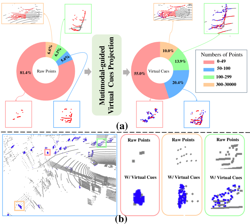
Figure 1: (a) Left: statistics of the number of points on nuScenes’s car. Right: the number of points on nuScenes’s car with multimodal-guided virtual cues. Raw points is red, the virtual cues is blue. (b) Virtual cues generated using MVCP scheme. Blue Square box: Virtual cues of a certain frame. The raw points are marked in gray, and the virtual cues are marked in blue.

F-Siamese [16] is the first multi-modal SOT tracker. It initially employs a 2D tracker to estimate the 2D bounding box of the target, which is then projected into the 3D viewing frustum. Subsequently, it introduces a frustum-based dual Siamese network that effectively reduces redundant point cloud area by combining 2D region proposals with the 3D search space, thereby improving tracking accuracy. However, F-Siamese overlooks the feature interactions between the different modalities, resulting in the loss of critical cues from dense images. Thus, its performance lags much behind LiDAR-Only methods. After that, MMF-Track [17] further enhances the semantic association between point clouds and images through multi-level feature interaction and fusion, significantly improving the model’s performance in sparse and occluded scenarios. However, its complex feature interaction module greatly limits the inference speed, which is crucial tracking tasks with real-time requirements.

Unlike the aforementioned methods that introduce additional visual branches to generate frustums or dense RGB features for semantic-texture fusion, we argue that directly leveraging virtual cues from the RGB image modality can effectively enhance the performance without incurring significant additional computational overhead. Notably, many existing object detection and segmentation methods [1, 18, 19] are lightweight and highly efficient, making them well-suited for use on resource-limited edge devices. These methods can maintain high perception performance while introducing minimal latency, making them particularly suitable for latency-sensitive tracking tasks. Building on this intuition, we propose a novel Multimodal-guided Virtual Cues Projection (MVCP) mechanism to enhance the density and completeness of point clouds, thereby mitigating the impact of sparse point cloud on accuracy and facilitating a better understanding of the surrounding environment. As shown in Fig1, we analyze the number of points in the nuScenes [20] dataset. It can be found that 81% of objects contain fewer than 50 points, while only 7% of objects have more than 300 points. This significant sparsity issue severely limits the tracking performance, as the few discriminative points on the target make it difficult to distinguish from the background. However, after applying our proposed Multimodal-guided Virtual Cues Projection (MVCP) mechanism, a significant change in the distribution of point clouds in the original dataset is observed. The proportion of objects with fewer than 50 points decreases from 81% to 55%, while the proportion of targets with more than 50 points rises from 19% to 45%.

Particularly, in our Multimodal-guided Virtual Cues Projection (MVCP) mechanism, a lightweight 2D object segmentor [1] is employed to crop the original point cloud into instance-wise frustums. Subsequently, dense 3D virtual cues are generated near these foreground points by lifting 2D pixels into 3D space, with depth completion used in the image space to infer the depth of these virtual cues. Finally, the MVCP combines the virtual cues with the original LiDAR measurements as input to a 3D SOT tracker [21]. Based on MVCP scheme, we construct our MVCTrack framework, which offers three key advantages: (1) Lightweight 2D object detection The 2D object detectors employed are well-optimized [1, 19], ensuring that their integration does not incur significant computational overhead while effectively leveraging dense visual features. (2) Balanced point density distribution: The virtual cues balance the density distribution of points across different distances, reducing the density imbalance between near and far objects. (3) Plug-and-play module: Our projection mechanism serves as a plug-and-play module that can be integrated with any existing or new advanced 2D or 3D detectors yielding substantial benefits with minimal effort—achieving significant gains. We evaluate our MVCTrack on the large-scale nuScenes datasets [20]. Extensive experimental results demonstrate that our approach achieves competitive performance on the nuScenes dataset, significantly surpassing existing multi-modal 3D trackers. Our main contributions are summarized as follows:

• Multimodal-guided Virtual Cues Projection (MVCP). A novel plug-in scheme for generating virtual cues that leverages dense semantics from the images to compensate for the sparsity of point clouds.

• MVCTrack. An enhanced 3D single object tracking network that integrates virtual cues, enabling end-to-end training to improve overall tracking performance, particularly for small and distant objects.

• Our approach achieves competitive performance on the challenging large-scale nuScenes datasets. Extensive ablation studies demonstrate the effectiveness and generalization of the proposed methods.

II RELATED WORK

LiDAR-based 3D Single Object Tracking. Leveraging the insensitivity of LiDAR to illumination changes and its ability to capture accurate distance information, numerous works on LiDAR-based 3D single object tracking (3D SOT) have emerged. SC3D [22], as a pioneering work in 3D SOT, employs a Kalman filter to generate a set of candidate 3D bounding boxes and selects the one most similar to the template target as the predicted result. However, due to the time-consuming candidate generation process, SC3D is not an end-to-end framework and struggles to achieve real-time performance. To address these problems, P2B [7] introduced a target-specific feature matching framework and utilized VoteNet[23] to estimate the target center. Similarly, 3D-SiamRPN [8] implemented a region proposal network for object tracking. Building upon this foundation, BAT[11] incorporated box-aware information to enhance similarity features. PTT [2, 9] proposes the Point-Track-Transformer module to assign weights to crucial point cloud features. STNet[24] developed an iterative coarse-to-fine correlation network for robust correlation learning. GLT-T[25] introduced a global-local Transformer voting scheme to generate higher-quality 3D proposals. A series of follow-up methods [26, 24, 27, 28, 25, 29, 30, 31, 32] have also adopted appearance matching frameworks. In contrast to the appearance matching framework, M²Track [33] introduced a motion-centric framework that utilizes motion information rather than appearance for 3D SOT, achieving impressive results. Furthermore, M²Track++ [34] explored the performance with a semi-supervised setting. However, those methods are still limited by the sparsity of point cloud in single modal.

Multi-Model 3D Single Object Tracking. Multi-Model 3D SOT leverage the complementary nature of diverse sensor data, such as LiDAR and RGB, to achieve more robust and accurate tracking. F-Siamese[16] introduced a frustum-based dual Siamese network that extends 2D region proposals from RGB images into 3D space, effectively reducing redundant 3D search areas. By performing accuracy validation within the 3D frustum, F-Siamese maintained a certain success rate even in cases of sparse point clouds or target occlusion; however, it lacks feature-level alignment and exhibits relatively slow tracking speed. Subsequently, MMF-Track [17] proposed a multimodal, multi-level fusion approach that aligns RGB images and point clouds in 3D space through a spatial alignment module, facilitating feature-level interaction between geometric and texture information. Although the multi-layer feature interaction in MMF-Track enables robust tracking performance in complex environments, its intricate feature interaction process significantly constrains inference speed, particularly on onboard robotic platforms.

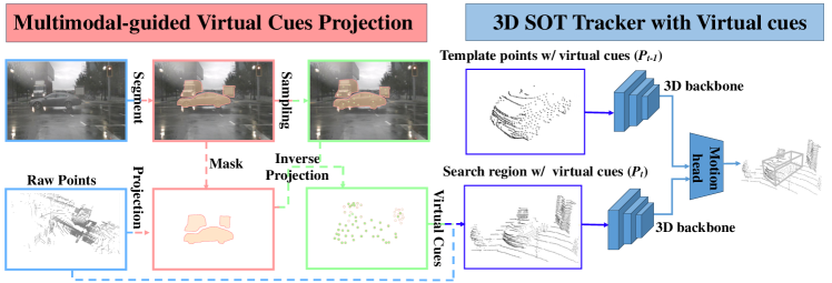
Figure 2: MVCTrack Framework. First step: Multimodal-guided virtual cues projection, this step will generate virtual cues based on the segmentation masks and raw points. Second step: 3D single object tracking with the integration of raw points and virtual cues.

III PRELIMINARY

3D Single Object Tracking In 3D SOT, given the point cloud input $P=\{(x_{i},y_{i},z_{i})\}$ at time $t$, where $(x_{i},y_{i},z_{i})$ denotes the 3D coordinates of a point. The 3D SOT task aims to predict the 3D bounding box of the tracked object $\mathbf{b}_{t}=(u,v,o,w,l,h,\theta)$, where $(u,v,o)$ represent the 3D center location, $w,l,h$ denote the width, length, and height of the object, and $\theta$ represents the rotation around the z-axis. The primary goal is to maintain a consistent tracking of the object across sequential frames by exploiting the spatio-temporal information provided by the point clouds.

2D-3D Correspondence In multi-modal fusion techniques, establishing a correspondence between 2D image and 3D point cloud data is essential for accurately integrating sensory information. The projection from 3D LiDAR measurements onto the 2D image plane involves several transformations. These transformations align the two modalities effectively, ensuring that each 3D point in the LiDAR frame is properly matched with its corresponding pixel in the 2D RGB image. Let $P=\{(x_{i},y_{i},z_{i})\}$ represent a point cloud. The mapping of 3D coordinates to 2D image pixels involves a series of homogeneous transformations. First, the LiDAR points undergo a transformation $T_{\text{car}\leftarrow\text{lidar}}$, which shifts the points from the LiDAR’s coordinate frame to the vehicle’s reference frame. Given that the vehicle may be moving, a time-dependent transformation $T(t_{1}\leftarrow t_{2})$ is applied to account for the displacement of the vehicle between the timestamps $t_{1}$ and $t_{2}$. After this, the transformed points are mapped from the vehicle’s reference frame to the RGB camera frame using $T_{\text{rgb}\leftarrow\text{car}}$. The final step is the application of the RGB camera’s intrinsic matrix $I_{\text{rgb}}$, which projects the 3D points onto the 2D image plane. The entire transformation process can be described as:

$$T_{t_{1}\leftarrow t_{2}}=T_{\text{rgb}\leftarrow\text{car}}\cdot T_{t_{1}\leftarrow t_{2}}\cdot T_{\text{car}\leftarrow\text{lidar}}$$ (1)

$$\mathbf{P}_{\text{rgb}}=I_{\text{rgb}}\cdot T_{t_{1}\leftarrow t_{2}}\cdot\mathbf{P}_{\text{lidar}}$$ (2)

IV METHOD

IV-A Overview

Given an initial bounding box $B_{0}=(x_{0},y_{0},z_{0},w,h,l,\theta_{0})\in\mathbb{R}^{7}$, where $(x_{0},y_{0},z_{0})$ denotes the object center, $(w,h,l)$ represent the object’s size, and $\theta_{0}$ indicates its orientation. Throughout tracking, we predict the target state $B_{f}=(x_{f},y_{f},z_{f},\theta_{f})\in\mathbb{R}^{4}$ for each frame $f$, because the size $(w,h,l)$ remains constant across frames. Our method leverages multi-modal virtual cues $v_{i}=(x,y,z)$, where $(x,y,z)$ specifies the 3D coordinates obtained from MVCP scheme. For each 2D object detection $b_{j}$ with an associated instance mask $m_{j}$, we generate a fixed number $\tau$ as virtual cues to compensate the sparsity of the point cloud.

IV-B Multimodal-guided Virtual Cues Projection

IV-B1 Virtual Cues Sampling

The process of virtual cues sampling begins with identifying potential areas around the tracked object where additional information may enhance the tracking performance. Given the inherent sparsity of LiDAR point clouds, particularly around small or distant objects, we aim to densely populate these regions with additional points that are not originally captured by the LiDAR sensor. To achieve this, we leverage 2D image data, which often provides more dense and detailed object boundaries, to inform the placement of virtual cues in the 3D space.

Typically, we obtain a set of 2D object segmentation masks $\mathbf{B}_{obj}=\{b_{1},b_{2},\dots,b_{n}\}$ from an 2D segmentor. Each detected object is represented by a bounding box $b_{j}=(u_{j},v_{j},w_{j},h_{j})$ and an associated instance mask $m_{j}$, which segments the object’s pixels in the 2D image. Using this mask, we generate a fixed number $\tau$ of virtual cues $\mathbf{v}_{i}=(x_{i},y_{i},z_{i})$ uniformly across the detected object’s area in the image, where $(x_{i},y_{i},z_{i})$ is the 3D location of generated virtual cues.

The virtual cues are sampled based on the pixel coordinates within the instance mask $m_{j}$, ensuring an even distribution of points throughout the object’s silhouette:

$$\mathbf{v}_{i}=\{(x_{i},y_{i},z_{i})\mid(x_{i},y_{i})\in m_{j},i=1,\dots,\tau\}\vspace{-2mm}$$ (3)

where $\tau$ is the sampled number of virtual cues per object.

IV-B2 Virtual Cues Projection

To project the virtual cues from 2D into 3D space, we use the LiDAR point cloud to infer depth. Each point $\mathbf{p}_{i}=(x_{i},y_{i},z_{i})$ from the LiDAR point cloud is first projected onto the 2D image plane, and for each virtual point $\mathbf{v}_{i}=(x_{i},y_{i},z_{i})$, we assign the depth value $d_{i}$ of its nearest neighbor LiDAR point in the projected 2D space:

$$d_{i}=\arg\min_{\mathbf{p}_{i}}\left\|\mathbf{v}_{i}-\mathbf{p}_{i}^{\text{2D}}\right\|\vspace{-2mm}$$ (4)

The virtual cues are unprojected back into the 3D space, ensuring that each virtual point $\mathbf{v}_{i}$ has a full 3D coordinate $(x_{i},y_{i},z_{i})$:

$$\mathbf{v}_{i}=\left(\frac{x_{i}}{z_{i}},\frac{y_{i}}{z_{i}},z_{i}\right)\vspace{-2mm}$$ (5)

As a result of the above process, the denser point cloud is generated, which effectively enhances the semantic information of discriminative points in scenes where real LiDAR point cloud may be sparse or incomplete. Here, we agree that adopting more advanced depth association methods could yield virtual cues with finer-grained geometric information. We remain this issue for future work.

TABLE I: Comparisons with state-of-the-art methods on nuScenes dataset [20]. L means LiDAR-Only methods. LC denotes LiDAR-Camera methods. M and S are motion-based and similarity-based paradigms. Success / Precision are used for evaluation. Bold and underline denote the best result and the second-best one, respectively. $\dagger$ means our reimplementation based on official code.

Tracker	Publish	Modality	Car [64,159]	Pedestrian [33,227]	Truck [13,587]	Trailer [3,352]	Bus [2,953]	Mean [117,278]
SC3D [22]	CVPR’19	L+S	22.31 / 21.93	11.29 / 12.65	30.67 / 27.73	35.28 / 28.12	29.35 / 24.08	20.70 / 20.20
P2B [7]	CVPR’20		38.81 / 43.18	28.39 / 52.24	42.95 / 41.59	48.96 / 40.05	32.95 / 27.41	36.48 / 45.08
PTT [9]	IROS’21		41.22 / 45.26	19.33 / 32.03	50.23 / 48.56	51.70 / 46.50	39.40 / 36.70	36.33 / 41.72
BAT [11]	ICCV’21		40.73 / 43.29	28.83 / 53.32	45.34 / 42.58	52.59 / 44.89	35.44 / 28.01	38.10 / 45.71
V2B [12]	NIPS’21		54.40 / 59.70	30.10 / 55.40	53.70 / 54.50	54.90 / 51.44	- / -	- / -
PTTR [26]	CVPR’22		51.89 / 58.61	29.90 / 45.09	45.30 / 44.74	45.87 / 38.36	43.14 / 37.74	44.50 / 52.07
M2Track [33]	CVPR’22		55.85 / 65.09	32.10 / 60.92	57.36 / 59.54	57.61 / 58.26	51.39 / 51.44	49.23 / 62.73
C2FT [35]	RAL’22		40.80 / 43.80	- / -	48.40 / 46.60	58.50 / 51.80	40.50 / 36.60	- / -
SMAT [36]	RAL’22		43.51 / 49.04	32.27 / 60.28	- / -	- / -	39.42 / 34.32	- / -
MLSET [37]	RAL’23		53.20 / 58.30	33.20 / 58.60	54.30 / 52.50	53.10 / 40.90	- / -	- / -
STTracker [38]	RAL’23		56.11 / 69.07	37.58 / 68.36	54.29 / 60.71	36.31 / 36.07	48.13 / 55.48	49.88 / 66.61
GLT-T [25]	AAAI’23		48.52 / 54.29	31.74 / 56.49	52.74 / 51.43	57.60 / 52.01	44.55 / 40.69	44.42 / 54.33
MoCUT [39]	ICLR’24		57.32 / 66.01	33.47 / 63.12	61.75 / 64.38	60.90 / 61.84	57.39 / 56.07	51.19 / 64.63
PTTR++ [40]	TPAMI’24		59.96 / 66.73	32.49 / 50.50	59.85 / 61.20	54.51 / 50.28	53.98 / 51.22	51.86 / 60.63
FlowTrack [41]	IROS’24		60.29 / 71.07	37.60 / 67.64	- / -	55.39 / 62.70	- / -	- / -
MMFTrack [17]	TIV’23	LC+S	50.73 / 58.51	32.80 / 66.25	- / -	- / -	52.73 / 52.78	- / -
Baseline [21]†	-	L+M	64.61 / 71.98	45.64 / 74.62	64.42 / 65.37	70.23 / 66.08	58.54 / 56.13	59.22 / 71.19
MVCTrack	Ours	LC+M	66.76 / 73.76	47.34 / 76.64	66.21 / 66.33	72.73 / 69.80	60.20 / 58.88	61.20 / 73.22
Improvement			$\uparrow$2.15 / $\uparrow$1.78	$\uparrow$1.70 / $\uparrow$2.02	$\uparrow$1.79 / $\uparrow$0.96	$\uparrow$2.50 / $\uparrow$3.72	$\uparrow$1.66 / $\uparrow$2.75	$\uparrow$1.98 / $\uparrow$2.03

IV-C MVCTrack with Virtual Cues

To validate the effectiveness of generated virtual cues for 3D SOT tasks, we integrate those virtual cues to enhance the detail of object boundaries by concatenating with the raw points. Specifically, the raw LiDAR point cloud $P=\{(x_{i},y_{i},z_{i})\}$ is combined with the virtual point cloud $\mathbf{V}=\{(x_{i},y_{i},z_{i})\}$, forming an augmented point cloud $\mathbf{P}^{\text{aug}}=P\cup\mathbf{V}$. Subsequently, the augmented point cloud are as follows:

$$\mathbf{P}^{\text{xyz}}=\left\{(x_{i},y_{i},z_{i})\mid(x_{i},y_{i},z_{i})\in P\cup\mathbf{V}\right\}\vspace{-2mm}$$ (6)

where $\quad\mathbf{P}^{\text{xyz}}\in\mathbb{R}^{n\times 3}$. The augmented point cloud $\mathbf{P}$ contains rich geometric and semantic information that effectively reduces noise interference and enhances the representation of target objects. The overall framework of MVCTrack is shown in Fig 2, where the augmented point cloud is input into a 3D convolutional network for encoding, capturing both spatial and semantic features of the objects. After the convolutional operations, the network transforms the extracted 3D feature map into a BEV feature map, which contains global spatial information about the object in the plane. Guided by virtual cues, the model can more clearly identify the central position, contour, and orientation angle $\theta$ of the target object in the BEV feature map, thereby improving the accuracy of the 3D bounding box. Finally, based on the BEV feature map, the model regresses the final 3D bounding box $B_{f}=(x_{f},y_{f},z_{f},\theta_{f})$ for the target object and achieves continues tracking in subsequent frames. Our MVCTrack not only compensates for deficiencies in sensor data but also significantly improve the tracking accuracy through explicitly multi-modal information fusion. More details about the tracking network can refer to  [21].

V EXPERIMENTS

V-A Dataset, Metrics and Implementation Details.

The extended range are defined as extended range [(-4.8,4.8),(-4.8,4.8),(-1.5,1.5)] and [(-1.92,1.92),(-1.92,1.92),(-1.5,1.5)] for cars and humans, respectively. The backbone of MVCTrack is designed with 4 sparse convolution blocks, each featuring 16, 32, 64, 128 channels, as the Shared backbone for efficient feature extraction. The tracking head is designed with 2 fully connected layers followed by a sigmoid activation function, which outputs the predicted center position and orientation. And we adopt a single regression loss to minimize the distance between predicted and ground truth center positions, along with an angular difference penalty for orientation. The entire MVCTrack network can be trained end-to-end. We train the model on two NVIDIA GTX 4090 GPUs for a total of 20 epochs using the AdamW optimizer, with a learning rate set to 1e-4 and a batch size of 256. The weight decay parameter is fixed at 1e-5. During training, we apply common data augmentation strategies such as random flipping, random rotation, and random translation. The loss function used is a single regression loss to refine the predicted outputs effectively. We follow the common setup [7, 33] and conduct extensive experiments on large-scale nuScenes [20] Dataset. The evaluation metrics is followed the common setup [2, 25, 42] to report Success and Precision based on one pass evaluation (OPE) [43, 44]. Our experiment video is available at https://youtu.be/c-OPJ0PvvbA video.

V-B Quantitative, Qualitative, and Ablation Study

Extensive results on nuScenes. We evaluate our MVCTrack on the large-scale nuScenes [20] dataset, known for its challenging and sparse point clouds. As shown in Tab. I, MVCTrack achieves significant improvements over prior methods and baseline, outperforming M²Track, which also uses motion cues, by 10.91%/8.67% and 15.23%/15.75% in Car and Pedestrian. Compared with the latest multi-modal tracking methods MMF-Track[17], MVCTrack outperforms 16.03%/15.25% and 14.53%/10.39% in the categories of Cars and Pedestrians. And MVCTrack also outperforms the baseline [21] without using virtual clues by 1.98%/2.03% in the mean accuracy, demonstrating the effectiveness of our multimodal-guided virtual cues Projection scheme.

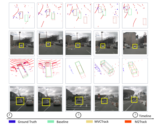
Figure 3: Visualization of tracking results on nuScenes dataset. We compare our MVCTrack with M²Track [33] and baseline model [21].

Ablation study of sampling strategy. MVCP is crucial for improving tracking accuracy in sparse scenarios. Therefore, we ablation the impact of different sampling strategies. Strategy 1: The sampling number of virtual points are generated based on the object’s distance from the sensor. Distant objects receive fewer points (with a minimum set to $\mathbf{\lambda}$), while closer objects receive more points (with a maximum set to $\mathbf{2\lambda}$). Strategy 2: Similar to Strategy 2, but with the converse trend: sparse objects at a distance receive more points (with a minimum set to $\mathbf{\lambda}$), while dense objects nearby receive fewer points (with a maximum set to $\mathbf{2\lambda}$). Strategy 3: A fixed number of virtual points $\mathbf{\lambda}$ is uniformly generated for all objects. As shown in Tab. II, Strategy 3 consistently exhibits the best performance, which we attribute to the fixed sampling number of virtual points being more similar with the real-world distribution of point clouds across varying distances.

TABLE II: Comparison for different sampling strategies.

Strategy	Category
	Car	Pedestrian
Strategy 1	64.53 / 72.92	45.59 / 74.64
Strategy 2	65.59 / 73.38	45.38 / 74.71
Strategy 3	66.76 / 73.76	47.34 / 76.64

The effectiveness on small objects. In Tab III, we perform the accuracy on small objects such as pedestrians, bicycle. Consistent with prior studies[33, 17, 41], small objects typically exhibit reduced point cloud representation, making tracking particularly challenging. However, our MVCTrack shows significant performance gains in these categories. By employing MVCP scheme, our MVCTrack effectively increases the point cloud density for small objects, leading to a notable accuracy improvement. This shows the effectiveness of our approach in handling small objects.

TABLE III: Comparison on small objects

Strategy/Method	Category
	Pedestrian	Bicycle
M2Track [33]	32.10 / 60.92	36.32 / 67.50
MMFTrack [17]	32.80 / 66.25	37.53 / 68.59
Ours	47.34 / 76.64	52.16 / 77.21
Improvement	$\uparrow$14.53 / $\uparrow$9.73	$\uparrow$14.53 / $\uparrow$9.73

TABLE IV: Comparison in long-distance scenarios.

Method	Distance Range	Category
		Car	Pedestrian
M2Track	$<30m$	68.73 / 77.14	44.44 / 73.33
	$\geqslant 30m$	57.24 / 64.92	34.14 / 60.89
Ours	$<30m$	73.23$\uparrow$3.28 / 80.42$\uparrow$10.80	55.24$\uparrow$4.50 / 83.00$\uparrow$9.67
	$\geqslant 30m$	67.62$\uparrow$10.38 / 73.74$\uparrow$8.82	49.14$\uparrow$15.0 / 78.44$\uparrow$17.55

The effectiveness in long-distance scenarios. Here, we classify the trajectories into different ranges based on the initial bbox location to evaluate the tracking performance in long-distance scenarios. As shown in Table V-B, our MVCTrack outperforms M²Track, which also uses motion cues, by 10.38%/8.82% and 15.00%/17.55% in Car and Pedestrian, demonstrating the effectiveness in long-distance scenes.

TABLE V: Comparison with different 2d images resolutions.

Resolutions	Category
	Car	Pedestrian
800 x 450	64.53 / 72.92	46.22 / 75.31
1600 x 900 (origin)	66.76 / 73.76	47.33 / 76.64

Robustness to 2D Segmentation. As shown in Tab V, We evaluate the robustness of our method against variations in the quality of 2D segmentation results by reducing the resolution of the input images. Specifically, we decrease the resolution from the original 1600x900 to half, simulating less accurate segmentation results. This experiment aims to evaluate the impact of decreased segmentation precision on the generation of virtual cues and overall tracking performance. Despite the significant reduction in image resolution, our method maintains a high accuracy, achieving a tracking success and precision of 64.53/72.92 and 46.22/75.31 in car and pedestrian, outperforming similar state-of-the-art models. These results indicate that our model demonstrates resilience to lower-quality segmentation inputs, suggesting that the MVCP mechanism effectively compensates for the diminished precision by generating robust virtual cues. This highlights the adaptability of our method, even when 2D segmentation results is compromised, further emphasizing its practical applicability in real-world scenarios where segmentation quality may fluctuate.

TABLE VI: Generalization ability on M2-Track.

Strategy /Method	Modality	Category
		Car	Pedestrian
M2Track	L+S	57.22 / 65.72	32.10 / 60.92
M2Track+VC	LC+M	58.15$\uparrow$1.93 / 66.88$\uparrow$2.16	36.64$\uparrow$4.54 / 65.28$\uparrow$4.36

Generalization Ability on Other Trackers. To demonstrate the generalization capability of the proposed MVCP scheme, we employ the generated virtual cues to representative M²Track [33]. As shown in Tab. V-B, the performance of M²Track improved significantly by 1.93%/2.16% and 4.54%/4.36% in Car and Pedestrian after incorporating generated virtual cues, strongly validating the effectiveness and generalization ability of our proposed MVCP mechanism. This result indicates that our MVCP method not only enhances MVCTrack but also provides substantial performance improvements for other state-of-the-art trackers. Furthermore, the plug-and-play feature of our approach enables seamless integration into existing LiDAR-based 3D SOT trackers, resulting in notable performance gains.

Running Speed. Our MVCTrack can achieve 32.1 FPS on single NVIDIA 3090Ti GPU and make certain improvement compared with 13.2 FPS of multi-modal MMFTrack [17].

Visualization results. As shown in Fig 3, we visualize the tracking results over the state-of-the-art method M2Track [33] and our baseline on the nuScenes [33] dataset, across diverse trajectories. In extremely sparse scenarios (rows 1 and 2), both M²Track (red bbox) and the baseline (green bbox) will fail to track. In contrast, our MVCTrack (yellow bbox) along with virtual cues is able to tightly track the target. In other case (rows 3 and 4), M²Track (red bbox) and the the baseline (green bbox) incorrectly track these similar objects due to insufficient points geometrics for differentiation. In comparison, our MVCTrack (yellow bbox) utilizes virtual cues to achieve robust tracking performance, closely aligning with the Ground Truth (blue bbox). The consistent robustness of MVCTrack, even in challenging sparse cases, shows its effectiveness for real-world scenes.

VI CONCLUSION

In this paper, to mitigate the inherent sparsity of point cloud, we propose a Multimodal-guided Virtual Cues Projection (MVCP) mechanism aimed at enhancing the performance of 3D SOT. Based on MVCP, we construct the MVCTrack framework, which directly utilizes the generated dense 3D virtual cues alongside the raw point cloud as input to the network. The proposed MVCTrack offers three key advantages: (1) Lightweight 2D object segmentation, ensuring efficient integration; (2) Balanced point density distribution, reducing the disparity between near and far objects; and (3) A plug-in module that can seamlessly integrate with existing trackers. Extensive Experiments demonstrate that MVCTrack achieves competitive performance on the nuScenes dataset, and significantly surpass existing multi-modal 3D trackers. We hope our research can provide new insights for 3D SOT.

References

- [1] X. Zhou, D. Wang, and P. Krähenbühl, “Objects as points,” in arXiv preprint arXiv:1904.07850, 2019.
- [2] J. Shan, S. Zhou, Z. Fang, and Y. Cui, “Ptt: Point-track-transformer module for 3d single object tracking in point clouds,” in 2021 IEEE/RSJ International Conference on Intelligent Robots and Systems (IROS). IEEE, 2021, pp. 1310–1316.
- [3] S. Zhou, Z. Tian, X. Chu, X. Zhang, B. Zhang, X. Lu, C. Feng, and Z. Jie, “Fastpillars: A deployment-friendly pillar-based 3d detector.”
- [4] A. Kim, A. Ošep, and L. Leal-Taixé, “Eagermot: 3d multi-object tracking via sensor fusion,” in Proceedings of the 2021 IEEE International Conference on Robotics and Automation (ICRA). IEEE, 2021, pp. 11 315–11 321.
- [5] J. Shan et al., “Real-time 3d single object tracking with transformer,” IEEE Transactions on Multimedia, vol. 25, pp. 2339–2353, 2022.
- [6] Y. Cui, Z. Fang, and S. Zhou, “Point siamese network for person tracking using 3d point clouds,” Sensors, vol. 20, no. 1, p. 143, 2019.
- [7] H. Qi, C. Feng, Z. Cao, F. Zhao, and Y. Xiao, “P2b: Point-to-box network for 3d object tracking in point clouds,” in Proceedings of the IEEE/CVF conference on computer vision and pattern recognition, 2020, pp. 6329–6338.
- [8] Z. Fang, S. Zhou, Y. Cui, and S. Scherer, “3d-siamrpn: An end-to-end learning method for real-time 3d single object tracking using raw point cloud,” IEEE Sensors Journal, vol. 21, no. 4, pp. 4995–5011, 2020.
- [9] J. Shan, S. Zhou, Y. Cui, and Z. Fang, “Real-time 3d single object tracking with transformer,” IEEE Transactions on Multimedia, vol. 25, pp. 2339–2353, 2022.
- [10] Y. Cui, Z. Fang, J. Shan, Z. Gu, and S. Zhou, “3d object tracking with transformer,” British Machine Vision Conference, pp. 1445–1458, 2021.
- [11] C. Zheng, X. Yan, J. Gao, W. Zhao, W. Zhang, Z. Li, and S. Cui, “Box-aware feature enhancement for single object tracking on point clouds,” in Proceedings of the IEEE/CVF International Conference on Computer Vision, 2021, pp. 13 199–13 208.
- [12] L. Hui, L. Wang, M. Cheng, J. Xie, and J. Yang, “3d siamese voxel-to-bev tracker for sparse point clouds,” Advances in Neural Information Processing Systems, vol. 34, pp. 28 714–28 727, 2021.
- [13] L. Bertinetto, J. Valmadre, J. F. Henriques, A. Vedaldi, and P. H. Torr, “Fully-convolutional siamese networks for object tracking,” in Computer Vision–ECCV 2016 Workshops: Amsterdam, The Netherlands, October 8-10 and 15-16, 2016, Proceedings, Part II 14. Springer, 2016, pp. 850–865.
- [14] B. Li, J. Yan, W. Wu, Z. Zhu, and X. Hu, “High performance visual tracking with siamese region proposal network,” in Proceedings of the IEEE conference on computer vision and pattern recognition, 2018, pp. 8971–8980.
- [15] J. Nie, Z. He, Y. Yang, M. Gao, and Z. Dong, “Learning localization-aware target confidence for siamese visual tracking,” IEEE Transactions on Multimedia, 2022.
- [16] H. Zou, J. Cui, X. Kong, C. Zhang, Y. Liu, F. Wen, and W. Li, “F-siamese tracker: A frustum-based double siamese network for 3d single object tracking,” in IEEE/RSJ International Conference on Intelligent Robots and Systems, 2020, pp. 8133–8139.
- [17] Z. Li et al., “Mmf-track: Multi-modal multi-level fusion for 3d single object tracking,” IEEE Transactions on Intelligent Vehicles, 2023.
- [18] C. Li et al., “Yolov6: A single-stage object detection framework for industrial applications,” arXiv preprint arXiv:2209.02976, 2022.
- [19] C.-Y. Wang, A. Bochkovskiy, and H.-Y. M. Liao, “Yolov7: Trainable bag-of-freebies sets new state-of-the-art for real-time object detectors,” in Proceedings of the IEEE/CVF Conference on Computer Vision and Pattern Recognition, 2023, pp. 7464–7475.
- [20] H. Caesar, V. Bankiti, A. H. Lang, S. Vora, V. E. Liong, Q. Xu, A. Krishnan, Y. Pan, G. Baldan, and O. Beijbom, “nuscenes: A multimodal dataset for autonomous driving,” in Proceedings of the IEEE/CVF conference on computer vision and pattern recognition, 2020, pp. 11 621–11 631.
- [21] J. Nie, F. Xie, S. Zhou, X. Zhou, D.-K. Chae, and Z. He, “P2p: Part-to-part motion cues guide a strong tracking framework for lidar point clouds,” arXiv e-prints, pp. arXiv–2407, 2024.
- [22] S. Giancola, J. Zarzar, B. Ghanem, S. Giancola, and J. Zarzar, “Leveraging shape completion for 3d siamese tracking,” in Proceedings of the IEEE/CVF conference on computer vision and pattern recognition, 2019, pp. 1359–1368.
- [23] C. R. Qi, O. Litany, K. He, and L. J. Guibas, “Deep hough voting for 3d object detection in point clouds,” in proceedings of the IEEE/CVF International Conference on Computer Vision, 2019, pp. 9277–9286.
- [24] L. Hui, L. Wang, L. Tang, K. Lan, J. Xie, and J. Yang, “3d siamese transformer network for single object tracking on point clouds,” in Computer Vision–ECCV 2022: 17th European Conference, Tel Aviv, Israel, October 23–27, 2022, Proceedings, Part II. Springer, 2022, pp. 293–310.
- [25] J. Nie, Z. He, Y. Yang, M. Gao, and J. Zhang, “Glt-t: Global-local transformer voting for 3d single object tracking in point clouds,” in Proceedings of the AAAI Conference on Artificial Intelligence, 2023, pp. 1957–1965.
- [26] C. Zhou, Z. Luo, Y. Luo, T. Liu, L. Pan, Z. Cai, H. Zhao, and S. Lu, “Pttr: Relational 3d point cloud object tracking with transformer,” in Proceedings of the IEEE/CVF Conference on Computer Vision and Pattern Recognition, 2022, pp. 8531–8540.
- [27] Z. Guo, Y. Mao, W. Zhou, M. Wang, and H. Li, “Cmt: Context-matching-guided transformer for 3d tracking in point clouds,” in Computer Vision–ECCV 2022: 17th European Conference, Tel Aviv, Israel, October 23–27, 2022, Proceedings, Part XXII. Springer, 2022, pp. 95–111.
- [28] Y. Xia, Q. Wu, W. Li, A. B. Chan, and U. Stilla, “A lightweight and detector-free 3d single object tracker on point clouds,” IEEE Transactions on Intelligent Transportation Systems, 2023.
- [29] J. Nie, Z. He, Y. Yang, Z. Bao, M. Gao, and J. Zhang, “Osp2b: One-stage point-to-box network for 3d siamese tracking,” in Proceedings of the Thirty-Second International Joint Conference on Artificial Intelligence, 2023, pp. 1285–1293.
- [30] K. Lan, H. Jiang, and J. Xie, “Temporal-aware siamese tracker: Integrate temporal context for 3d object tracking,” in Proceedings of the Asian Conference on Computer Vision, 2022, pp. 399–414.
- [31] T. Ma, M. Wang, J. Xiao, H. Wu, and Y. Liu, “Synchronize feature extracting and matching: A single branch framework for 3d object tracking,” in Proceedings of the IEEE/CVF International Conference on Computer Vision, 2023, pp. 9953–9963.
- [32] W. Xu, S. Zhou, and Z. Yuan, “Pillartrack: Redesigning pillar-based transformer network for single object tracking on point clouds,” arXiv preprint arXiv:2404.07495, 2024.
- [33] C. Zheng, X. Yan, H. Zhang, B. Wang, S. Cheng, S. Cui, and Z. Li, “Beyond 3d siamese tracking: A motion-centric paradigm for 3d single object tracking in point clouds,” in Proceedings of the IEEE/CVF Conference on Computer Vision and Pattern Recognition, 2022, pp. 8111–8120.
- [34] ——, “An effective motion-centric paradigm for 3d single object tracking in point clouds,” IEEE Transactions on Pattern Analysis and Machine Intelligence, 2023.
- [35] B. Fan, K. Wang, H. Zhang, and J. Tian, “Accurate 3d single object tracker with local-to-global feature refinement,” IEEE Robotics and Automation Letters, 2022.
- [36] Y. Cui, J. Shan, Z. Gu, Z. Li, and Z. Fang, “Exploiting more information in sparse point cloud for 3d single object tracking,” IEEE Robotics and Automation Letters, vol. 7, no. 4, pp. 11 926–11 933, 2022.
- [37] Q. Wu, C. Sun, and J. Wang, “Multi-level structure-enhanced network for 3d single object tracking in sparse point clouds,” IEEE Robotics and Automation Letters, 2023.
- [38] Y. Cui, Z. Li, and Z. Fang, “Sttracker: Spatio-temporal tracker for 3d single object tracking,” IEEE Robotics and Automation Letters, 2023.
- [39] J. Nie, Z. He, X. Lv, X. Zhou, D.-K. Chae, and F. Xie, “Towards category unification of 3d single object tracking on point clouds,” in The Twelfth International Conference on Learning Representations, 2024.
- [40] Z. Luo, C. Zhou, L. Pan, G. Zhang, T. Liu, Y. Luo, H. Zhao, Z. Liu, and S. Lu, “Exploring point-bev fusion for 3d point cloud object tracking with transformer,” IEEE Transactions on Pattern Analysis and Machine Intelligence, 2024.
- [41] S. Li, Y. Cui, L. Zhiheng, and Z. Fang, “Flowtrack: Point-level flow network for 3d single object tracking,” arXiv preprint arXiv:2407.01959, 2024.
- [42] T.-X. Xu, Y.-C. Guo, Y.-K. Lai, and S.-H. Zhang, “Mbptrack: Improving 3d point cloud tracking with memory networks and box priors,” arXiv preprint arXiv:2303.05071, 2023.
- [43] Y. Wu, J. Lim, and M.-H. Yang, “Online object tracking: A benchmark,” in Proceedings of the IEEE conference on computer vision and pattern recognition, 2013, pp. 2411–2418.
- [44] M. Kristan, J. Matas, A. Leonardis, T. Vojíř, R. Pflugfelder, G. Fernandez, G. Nebehay, F. Porikli, and L. Čehovin, “A novel performance evaluation methodology for single-target trackers,” IEEE transactions on pattern analysis and machine intelligence, vol. 38, no. 11, pp. 2137–2155, 2016.