DYffCast: Regional Precipitation Nowcasting Using IMERG Satellite Data. A case study over South America
Abstract
Climate change is increasing the frequency of extreme precipitation events, making weather disasters such as flooding and landslides more likely. The ability to accurately nowcast precipitation is therefore becoming more critical for safeguarding society by providing immediate, accurate information to decision makers. Motivated by the recent success of generative models at precipitation nowcasting, this paper: extends the DYffusion framework to this task and evaluates its performance at forecasting IMERG satellite precipitation data up to a 4-hour horizon; modifies the DYffusion framework to improve its ability to model rainfall data; and introduces a novel loss function that combines MSE, MAE and the LPIPS perceptual score. In a quantitative evaluation of forecasts up to a 4-hour horizon, the modified DYffusion framework trained with the novel loss outperforms four competitor models. It has the highest CSI scores for weak, moderate, and heavy rain thresholds and retains an LPIPS score 0.2 for the entire roll-out, degrading the least as lead-time increases. The proposed nowcasting model demonstrates visually stable and sharp forecasts up to a 2-hour horizon on a heavy rain case study111Code is available at https://github.com/Dseal95/DYffcast.
1 Introduction
The ability to accurately nowcast (predict up to 6 hours in advance [1]) precipitation, is a vital task that can help mitigate hazards such as flooding or landslides [2]. Globally, heavy precipitation events are becoming more common due to climate change [3, 4, 5, 6, 7], causing large human displacement, human fatalities [8], and economic cost. Accurate precipitation forecasts are therefore becoming more instrumental in providing critical information required for weather-dependent decision making that can safeguard society. The absence of effective precipitation models especially impacts countries that lack access to freely available ground-based radar systems and experience vulnerability in resource management, agriculture, disaster preparedness, and climate adaptation.
This work evaluates the applicability of a novel probabilistic, spatio-temporal forecasting framework, DYffusion [9], to precipitation nowcasting. This research is motivated by the recent success of generative modelling at this task and, DYffusion’s skilful forecasts over long horizons on Navier-Stokes flows and sea surface temperatures (SST); two systems that exhibit complex dynamics comparable to that of precipitation. In this study, the focus is on how well DYffusion can forecast up to a 4-hour horizon, how well these forecasts compare to deterministic and statistical baselines, and what modifications are required to apply DYffusion to precipitation nowcasting.
The contributions to the field of precipitation nowcasting can be summarised as follows:
-
1.
Evaluation of a novel modelling framework, alternative to diffusion-based or Generative Adversarial Network (GAN)-based models, at precipitation nowcasting.
-
2.
A focus on countries lacking freely available ground-based radar and most impacted by global warming.
-
3.
Introduction of a novel loss function that demonstrates how guiding a pixel-wise distance-based loss with a perceptual loss improves a model’s ability to learn small-scale features in imbalanced datasets such as precipitation.
2 Methods
2.1 Data
This research uses the publicly available satellite precipitation product, IMERG. In particular, it uses the latest version (V07B [10]) of the half-hourly, Early Run product with a spatial resolution and precipitation rates in . The dataset is created from four 128128 grid boxes that cover the South American countries: Colombia, Ecuador and Perú. These are regions that are susceptible to increased flooding and have limited availability of weather radar222According to the World Meteorological Organisation’s (WMO) radar database, South America has roughly / of North America’s or Europe’s radar [11].. The four 128128 grid boxes are stacked into dimensions: (N, S, C, H, W) where N is the number of samples, S is the sequence length (input and target) and C is the number of channels (1 for IMERG). The data is preprocessed to using linear normalisation, transform and min-max normalisation. For this research, a 4-hour horizon or 81128128 images, was chosen to match the latency of the Early-Run IMERG product and avoid any discontinuity of real-time data.
2.2 Modelling
2.2.1 DYffusion Framework
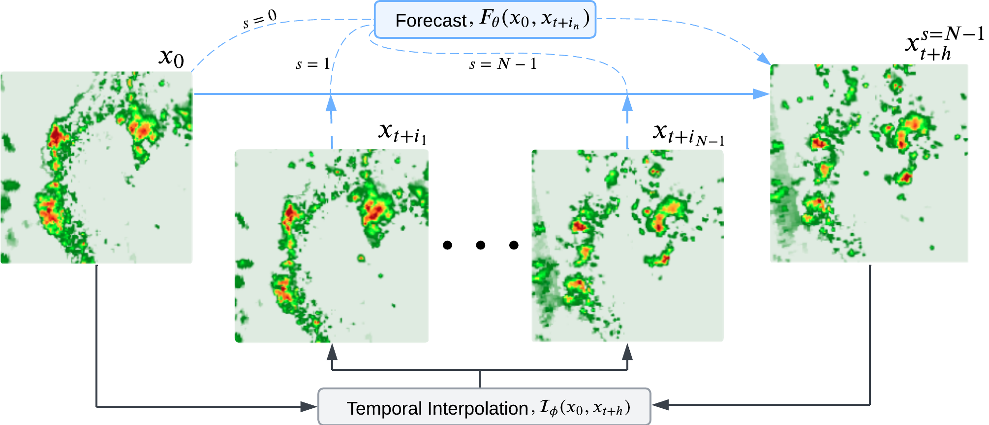
The DYffusion framework is outlined in Figure 1. It consists of an Interpolator network, and a Forecastor network, .
Training. is trained to interpolate any timestep of the sequence , given the initial and final states, and , respectively. is trained to forecast the horizon given the initial condition and an intermediate state . This two-stage training has a constant memory footprint as a function of , only requiring and (plus during the Interpolator training).
Inference. Given an initial condition, , the entire sequence is generated over (or ) auto-regressive steps. At step = ( = + 1), predicts the horizon using only . then interpolates using and . At the next step ( = ), predicts the horizon again , using and . and are then used to interpolate, . This process is repeated until predicts ( times), using the nearest intermediate value, . This iterative process is analogous to the iterative denoising in standard diffusion models and underpins the time-coupled, DYnamics informed nature of the DYffusion framework. The final forecast is the mean of an ensemble of members.
The probabilistic nature of DYffusion occurs through Monte Carlo dropout. is trained with dropout rates that are enabled during the training (and inference) of . Enabling dropout during training is analogous to interpolating by sampling it from the conditional probability distribution .
2.2.2 DYffusion Key Modifications
For the IMERG dataset, the SST U-Net backbone from DYffusion and parts of the training framework were modified to model the rainfall data. The following key modifications were made:
-
1.
Loss Function. Replaced the L1 loss with a novel loss function (referred to as LCB), combining the Learned Perceptual Image Patch Similarity (LPIPS)[12] score with the class-weighted Mean Squared Error (MSE) and Mean Absolute Error (MAE) loss proposed in [13] (referred to as CBLoss in [14]). LCB was constructed as follows:
(1) Based on experimental results during Interpolator training, was set to 0.6, optimising for MSE, LPIPS and Critical Success Index (CSI) at varying thresholds. This value slightly biases the CBLoss towards spatial accuracy, while the perceptual component prevents large-scale features from dominating and improves image detail. Lower values ( 0.6) led to background artefacts and magnitude errors. For the CBLoss, the scaling term was set to 1.0 to equally weight the MSE and MAE components, and the rainfall classes (in ) and their associated weights were:
(2) -
2.
Forecastor Training. Removed any exposure to the horizon during Forecastor training to better emulate the sampling process. Referring to Algorithm 1, Stage 2, Step 2 in the original DYffusion paper, the intermediate values are now interpolated using the initial condition and an initial forecast instead of the target . This initial forecast is generated using only the initial conditions () to directly replicate the sampling procedure. A separate loss term for the initial forecast is added to the existing loss in Stage 2, Step 3 of Algorithm 1 in the original DYffusion paper. The updated loss function (including the one-step-ahead loss) becomes:
(3) Where L represents the loss function and is used to balance the different terms. For training, a linear schedule is used to calculate , starting at (decaying to 0 over 20 epochs) to place more emphasis on the initial forecast at the start of training. and are both set to 0.5, inherited from the original DYffusion implementation.
-
3.
Cold Sampling. Clamped the cold sampling update to avoid passing the Interpolator data . The cold sampling update from Algorithm 2, Step 4 in the original DYffusion paper becomes:
(4)
2.2.3 Baselines
We compare DYffusion to auto-regressive implementations of both deterministic and statistical methods to align more closely with DYffusion’s roll-out inference:
-
•
ConvLSTM [15]: implemented the same 2-layer architecture used on the Radar Echo dataset, but with increased hidden states (128 vs 64), larger kernels (55 vs 33), and additional pixel-wise dropout (either 0.15 or 0.4) after each ConvLSTM cell for regularisation. The ConvLSTM was trained to predict the next timestep from the previous 41128128 images (2 hours).
-
•
Short-Term Ensemble Prediction System (STEPS)[16]: implemented in PySteps [17] following the STEPS example on the PySTEPS website333https://pysteps.readthedocs.io/en/stable/auto_examples/plot_steps_nowcast.html. The previous 41128128 images (2 hours) were used as input and the units were transformed from to dBR before estimating the motion field and forecasting the next timestep.
3 Results
| Model | MSE | LPIPS | CSI2 | CSI10 | CSI18 | CRPS | SSR | Time [s] |
|---|---|---|---|---|---|---|---|---|
| DYffusion | 0.0020 | 0.145 | 0.270 | 0.112 | 0.064 | 0.013 | 0.131 | 3 |
| DYffusion | 0.0015 | 0.323 | 0.227 | 0.068 | 0.023 | 0.010 | 0.050 | 3 |
| ConvLSTM | 0.0085 | 0.272 | 0.139 | 0.027 | 0.010 | 1.2 | ||
| ConvLSTM | 0.0052 | 0.335 | 0.165 | 0.038 | 0.016 | 1.2 | ||
| STEPS | 2.4102 | 0.342 | 0.140 | 0.030 | 0.011 | 0.013 | 0.219 | 2.1 |
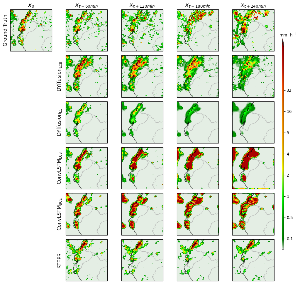
Table 1 shows the 4-hour averaged forecast evaluation metrics for each of the models on the test dataset. For both DYffusion and the baseline ConvLSTM [15], two models were trained. One model was trained using the LCB loss and a second model was trained using the model’s native loss function: L1 loss for DYffusion and binary cross-entropy (BCE) loss for ConvLSTM. The DYffusion and STEPS models are evaluated by taking the mean prediction from a 10-member ensemble. Figure 2 demonstrates each model’s nowcasting ability on the heavy precipitation event, Cyclone Yaku [18]. The forecasts clearly show the improved sharpness, detail and stability of DYffusion, especially up to a 2-hour horizon. This is supported by its outperforming CSI and LPIPS scores in Table 1. DYffusion can distinguish between heavy rain intensities in the band of rain moving toward the coast, and it tracks the split at the top of the rain-band forming at around min. The ConvLSTM also demonstrates improved sharpness (at earlier timesteps) compared to the ConvLSTM, indicating the effectiveness of the LCB loss function at capturing the small-scale features. DYffusion more accurately forecasts Cyclone Yaku’s spatial expansion compared to STEPS. However, Figure 2 shows that optical flow methods remain effective at earlier timesteps, before chaotic behaviour emerges.
Computational Resources.
DYffusion was trained on an NVIDIA L4 GPU, which is readily accessible through cloud computing vendors at reasonable costs. Training took 20 minutes per epoch for the Interpolator (60 epochs, 20 hours total) and 1.5 hours per epoch for DYffusion with a 10-member ensemble (25-30 epochs, 40 hours total). The IMERG dataset requires 18GB of storage.
4 Conclusion
In this study, DYffusion has been extended to the task of precipitation nowcasting. The task was to forecast IMERG precipitation data at 30-minute intervals up to a 4-hour horizon, generating a total of 81128128 images. By applying key modifications to the DYffusion framework and introducing a novel loss function, the modified framework outperforms both deterministic (ConvLSTM) and statistical (STEPS) baselines. Overall, the initial results of DYffusion suggest that with some improvements, the DYffusion framework is a potential candidate for operational precipitation nowcasting. The constant memory footprint associated with the forecast-interpolate process makes it an attractive alternative to single-pass generative networks.
Limitations.
Nowcasting precipitation is more challenging than SST or Navier-Stokes. The initial task of forecasting the 4-hour horizon from a single timestep is difficult. The implemented U-Net backbone struggles to not forecast as an expansion or reduction of the initial condition . This ultimately constrains the problem to the spatial domain of , contributing to the limited variability in the ensemble forecasts.
Future Work.
The results of [19] demonstrate the importance of high SSR scores for more skilful precipitation nowcasts. Conditioning the initial forecast with atmospheric information, such as divergence at 925 hPa and wind speed, is an interesting avenue to explore. The additional physical context should help the model capture the non-linear chaotic evolution of the rainfall, especially at earlier timesteps, similar to the motion field in STEPS. This should improve and, therefore, the overall stochasticity by allowing the framework to sufficiently explore .
References
- [1] Wang Y, et al. Guidelines for Nowcasting Techniques. World Meteorological Organization; 2017. P. 11.
- [2] Tohari A. Study of rainfall-induced landslide: a review. IOP Conference Series: Earth and Environmental Science. 2018 feb;118(1):012036. Available from: https://dx.doi.org/10.1088/1755-1315/118/1/012036.
- [3] Donat M, Lowry A, Alexander L, et al. More extreme precipitation in the world’s dry and wet regions. Nature Climate Change. 2016;6:508-13. Available from: https://doi.org/10.1038/nclimate2941.
- [4] Kendon EJ, Fischer EM, Short CJ. Variability conceals emerging trend in 100yr projections of UK local hourly rainfall extremes. Nature Communications. 2023;14:1133. Available from: https://doi.org/10.1038/s41467-023-36499-9.
- [5] Myhre G, Alterskjær K, Stjern CW, et al. Frequency of extreme precipitation increases extensively with event rareness under global warming. Scientific Reports. 2019;9:16063. Available from: https://doi.org/10.1038/s41598-019-52277-4.
- [6] Robinson A, Lehmann J, Barriopedro D, et al. Increasing heat and rainfall extremes now far outside the historical climate. npj Climate and Atmospheric Science. 2021;4:45.
- [7] Tabari H. Climate change impact on flood and extreme precipitation increases with water availability. Scientific Reports. 2020;10:13768. Available from: https://doi.org/10.1038/s41598-020-70816-2.
- [8] for the Coordination of Humanitarian Affairs (OCHA) UNO. OCHA, editor. Latin America & The Caribbean Weekly Situation Update as of 1 March 2024. OCHA; 2024. Accessed: 2024-03-01. https://reliefweb.int/report/bolivia-plurinational-state/latin-america-caribbean-weekly-situation-update-1-march-2024.
- [9] Cachay SR, Zhao B, James H, Yu R. Dyffusion: A dynamics-informed diffusion model for spatiotemporal forecasting. arXiv preprint arXiv:230601984. 2023.
- [10] Huffman GJ, Bolvin DT, Joyce R, Kelley OA, Nelkin EJ, Portier A, et al. IMERG V07 Release Notes. NASA; 2023. Available from: https://gpm.nasa.gov/sites/default/files/2024-02/IMERG_V07_ReleaseNotes_240221.pdf.
- [11] Organization WM. WMO, editor. WMO Radar Database [Database]. WMO; 2019. Accessed: March 2019. Available from: http://wrd.mgm.gov.tr/.
- [12] Zhang R, Isola P, Efros AA, Shechtman E, Wang O. The Unreasonable Effectiveness of Deep Features as a Perceptual Metric. CoRR. 2018;abs/1801.03924. Available from: http://arxiv.org/abs/1801.03924.
- [13] Shi X, et al. Deep Learning for Precipitation Nowcasting: A Benchmark and a New Model. In: Advances in Neural Information Processing Systems. vol. 30. NeurIPS; 2017. p. 5617-27.
- [14] Kim W, Jeong CH, Kim S. Improvements in deep learning-based precipitation nowcasting using major atmospheric factors with radar rain rate. Computers & Geosciences. 2024;184:105529. Available from: https://www.sciencedirect.com/science/article/pii/S0098300424000128.
- [15] Shi X, Chen Z, Wang H, Yeung D, Wong W, Woo W. Convolutional LSTM Network: A Machine Learning Approach for Precipitation Nowcasting. CoRR. 2015;abs/1506.04214. Available from: http://arxiv.org/abs/1506.04214.
- [16] Bowler NE, Pierce CE, Seed AW. STEPS: A probabilistic precipitation forecasting scheme which merges an extrapolation nowcast with downscaled NWP. Quarterly Journal of the Royal Meteorological Society. 2006;132:2127-55. Available from: https://doi.org/10.1256/qj.04.100.
- [17] Pulkkinen S, Nerini D, Pérez Hortal AA, Velasco-Forero C, Seed A, Germann U, et al. Pysteps: An open-source Python library for probabilistic precipitation nowcasting (v1. 0). Geoscientific Model Development. 2019;12(10):4185-219.
- [18] Adam Voiland. Observatory NE, editor. Warming Water and Downpours in Peru. NASA Earth Observatory; 2023. Accessed [Insert Date]. Available from: https://earthobservatory.nasa.gov/images/151183/warming-water-and-downpours-in-peru.
- [19] Nai C, Pan B, Chen X, Tang Q, Ni G, Duan Q, et al. Reliable precipitation nowcasting using probabilistic diffusion models. Environmental Research Letters. 2024 feb;19(3):034039. Available from: https://dx.doi.org/10.1088/1748-9326/ad2891.