Scalar embedding of temporal network trajectories

Abstract

A temporal network –a collection of snapshots recording the evolution of a network whose links appear and disappear dynamically– can be interpreted as a trajectory in graph space. In order to characterize the complex dynamics of such trajectory via the tools of time series analysis and signal processing, it is sensible to preprocess the trajectory by embedding it in a low-dimensional Euclidean space. Here we argue that, rather than the topological structure of each network snapshot, the main property of the trajectory that needs to be preserved in the embedding is the relative graph distance between snapshots. This idea naturally leads to dimensionality reduction approaches that explicitly consider relative distances, such as Multidimensional Scaling (MDS) or identifying the distance matrix as a feature matrix in which to perform Principal Component Analysis (PCA). This paper provides a comprehensible methodology that illustrates this approach. Its application to a suite of generative network trajectory models and empirical data certify that nontrivial dynamical properties of the network trajectories are preserved already in their scalar embeddings, what enables the possibility of performing time series analysis in temporal networks.

1 Introduction

If complexity emerges out of the interactions of elements, then it is safe to say that Network Science [1, 2] studies the architecture of complexity. In a nutshell, the interaction backbone of complex systems can be mathematically modeled as graphs, or more generally networks if these graphs model real-world interactions (from now on we will use the terms graph and network in an interchangeable way). In many occasions, these interactions can vary dynamically, and, accordingly, networks can evolve over time. The area of temporal networks [3, 4, 5, 6] englobes such idea, and usually focus on understanding how dynamical processess –from diffusion [7, 8, 9], social [10] or financial interactions [11] to epidemic spreading [12, 13], brain activity [14] or even propagation of delays in the air transport system [15, 16]– are affected when the network changes over time [17]. While the field has been predominantly driven by studies of the dynamics on the network, more recently some focus has been paid to study, from a principled viewpoint, the intrinsic dynamics of temporal networks. The rationale is that, to make use of the toolkit of dynamical systems, time series analysis and signal processing as a means to characterize the intrinsic dynamics of a temporal network, it is helpful to interpret such temporal network as a network trajectory [18].

One direction to deal with network trajectories is to develop methods that extend classical properties of time series to the network realm. In this line, classical dynamical concepts such as linear correlation functions [18, 19, 20, 21], Lyapunov exponents [22, 23], or memory [24] have recently been extended to temporal networks. The opposite direction, followed in this work, is to convert network trajectories into low-dimensional signals where classical methods can be readily applied. In this case, it is clear that simple symbolization cannot work due to high dimensionality [24], and thus we need to resort to embedding techniques. Traditional graph embedding methods leverage dimensionality reduction techniques to build a projection of the nodes (or edges [25]) of a single, static network in a (low-dimensional) space. Techniques include Laplacian eigenmaps [26], locally linear embedding [27], and graph factorization [28] among others (see [29] and references therein for a review). Extensions of these ideas to temporal networks have predominantly focused again on projecting nodes [30, 31]. Interestingly, only very recently some approaches [32, 33] have been proposed to project full network snapshots –rather than individual nodes or edges–. The rationale for projecting network snapshots rather than their microscopic properties is that each snapshot, conceived as a point in graph space, can somehow be seen as lacking internal structure [18]. Moreover, if one aims to do time series analysis –or signal processing– of network trajectories, then the key aspect of the network trajectory to be preserved in the embedding is the relation between snapshots, rather than the relation between the nodes or edges of each snapshot. Such insight suggests considering quasi-isometric transformations of the temporal network, and in particular, recently lead to the proposal [32] that explores the performance of multidimensional scaling (MDS) embedding of a specific model of temporal networks called tie-decay networks [32, 34, 35]. However, these works do not explicitly address whether low-dimensional embedding preserves key statistical properties of network trajectories, and to which extent standard concepts like memory, temporal correlations or dynamical instability can be retrieved from such low-dimensional embeddings.

Here we expand on [32] to consider various possible approaches one can follow to obtain low-dimensional –and in particular, scalar– embeddings of network trajectories using linear dimensionality reduction methods. We build various types of complex dynamics, from one-dimensional processes to synthetic network trajectories –white, noisy periodic, autorregressive and chaotic– and empirical temporal networks, and explore how correctly the resulting embeddings capture the subtle, intrinsic dynamics of the original network trajectory. The rest of the paper goes as follows. In Sec. 2 we define our methodology, which encompasses four strategies to obtain low-dimensional (and in particular, scalar) embeddings of network trajectories that leverage two different dimensionality reduction philosophies: principal component analysis and multidimensional scaling. In this section we also define the metrics used to validate our results, which include autocorrelation functions, Lyapunov exponents, and their extensions for network trajectories. In Sec. 3 we describe the results of applying the embedding methodology to signals of different complexity, ranging from 1D processes to synthetic temporal network models. We also apply the method to a couple of empirical temporal networks, in order to showcase how the method works in real scenarios. In Sec. 4 we conclude and discuss open problems for future work.

2 Methodology

Let us define a temporal network –or network trajectory– as an ordered sequence of $T$ graphs ${\cal S}=(G_{1},G_{2},\dots,G_{T})$, where $G_{t}$ is the $t$-th network snapshot. When the nodes are labelled, $G_{t}$ can be fully represented by its adjacency matrix ${\bf A}(t)$, with entries $A_{ij}(t)$. We assume that each network snapshot has a fixed number of nodes $N$ and let the time-evolving interactions be weighted or directed in general. We define the low-dimensional Euclidean embedding of such trajectory as a time series ${\cal S}_{\Phi}:=\{z_{1},z_{2},\dots,z_{T}\}$, where $z_{t}\in\mathbb{R}^{\textsc{dim}}$, and in general we aim at $\textsc{dim}\ll T$ ($\textsc{dim}=1$ is the case of special interest that produces a scalar embedding). Accordingly, the embedding function $\Phi:G_{t}\to z_{t}$ assigns a point $z\in\mathbb{R}^{\textsc{dim}}$ to every graph: $z=\Phi(G),\ \forall\ G\in{\cal S}$. The whole problem therefore reduces to find the function $\Phi(\cdot)$.

In this work, we construct functions $\Phi(\cdot)$ based on linear dimensionality reduction schemes. In particular, we consider four strategies to build $\Phi(\cdot)$ based either on PCA or MDS. The proposed methods are conceptually similar to each other, since all apply a dimensional reduction to the network trajectory, but differ in a few technical details which produce some variability in the results and highlight different aspects of the problem.

2.1 PCA-based strategies

Principal Component Analysis (PCA) is a widely used linear dimensionality reduction technique that identifies orthogonal directions along which the variance of the data is maximized [36]. Formally, PCA involves the spectral decomposition of a covariance matrix of data features in terms of the eigenvalues (which capture the magnitude of the explained variance) and the associated eigenvectors (the principal components).

In order to apply PCA to our problem, the network snapshots $G_{t}$ are originally projected in a suitable (Euclidean) feature space. Now, which would be the feature vector of each network snapshot? Shall we just extract a list of network scalar metrics associated to each snapshot or shall we use all the entries of the adjacency matrix as features? The key insight is to realize that, for the sake of understanding the properties of a network trajectory (i.e. the dynamics of a temporal network), the most relevant properties of each network snapshot are not necessarily their individual topological properties, but the relative positions among snapshots. In other words, an intuitive solution is to consider the set of relative distances between a snapshot $G_{t}$ and every other snapshot as the features of snapshot $G_{t}$. Accordingly, $G_{t}$ is expressed as a vector of $T$ features, where the $j$-th feature depicts the distance between $G_{t}$ and the $j$-th network snapshot. Subsequently, one can project $G_{t}$ in such a feature space, where the first axis relates to the distance of a generic snapshot $G_{t}$ to $G_{1}$, the second axis to the distance to $G_{2}$, and so on. By taking the spectral decomposition of the distance-based covariance matrix and projecting the data points into the first principal component (or by simply using the first component), we obtain a scalar embedding of the network trajectory.

More specifically, we first define the features of each network snapshot based on pairwise squared distances. From pairs of snapshots $G_{t}$ and $G_{\ell}$, we construct the squared distance matrix:

$$\mathcal{D}^{(2)}=\{d_{t\ell}^{2}\}_{t,\ell=1}^{T},\quad d_{t\ell}^{2}=\|G_{t}-G_{\ell}\|^{2},$$ (1)

where $\|\cdot\|$ is a suitable norm (e.g., Frobenius or an $L_{p}$ norm for adjacency matrices). While using standard distances $d_{ij}$ already produces decent results in our problem, squared distances are a better choice because they have a direct relationship with the inner product space and preserve better the distances after the spectral decomposition is applied (as clarified in the MDS section). Before applying such decomposition, in PCA the covariance matrix must be column-centered, such that features have zero mean and variance can be maximized along the principal components [36]:

$$\tilde{\mathcal{D}}_{t\ell}^{(2)}=d_{t\ell}^{2}-\langle d_{t\ell}^{2}\rangle_{\ell},$$ (2)

where $\langle d_{t\ell}^{2}\rangle_{\ell}$ is the mean over columns. The column-centered matrix $\tilde{\mathcal{D}}^{(2)}$ serves as the input feature space for PCA. Since the covariance matrix $\tilde{{\cal D}}^{{(2)}^{\top}}\tilde{{\cal D}}^{(2)}$ is always symmetric and positive definite, the spectral decomposition:

$$\tilde{{\cal D}}^{(2)^{\top}}\tilde{{\cal D}}^{(2)}=\sum_{i=1}^{T}\Lambda_{i}{\bf e}_{i}{\bf e}_{i}^{\top}$$ (3)

has always non-negative eigenvalues which can be ordered as $\Lambda_{1}\geq\Lambda_{2}\geq\dots\geq\Lambda_{T}\geq 0$ and $T$ associated orthogonal and real eigenvectors, where ${\bf e}_{i}=(e^{1}_{i},e^{2}_{i},\dots,e^{T}_{i})$ is the $i$-th eigenvector –also called the $i$-th principal component– with entries $e_{i}^{j}\in\mathbb{R}$. Reducing the dimensionality of each network snapshot $G_{t}$ from $T$ (the original dimension of the feature set) to $\textsc{dim}\ll T$ implies truncating this decomposition at order dim. From this point, we identify two slightly different strategies of finding a low-dimensional embedding of the network trajectory $\cal S$:

i) PCA-projection strategy: The most conventional approach in PCA is to systematically project the feature vector of each network snapshot onto the first dim principal components. If we label ${\bf v}_{t}$ as the feature vector of $G_{t}$ (the $t$-th row in $\tilde{{\cal D}}^{(2)}$), then $z_{t}=({\bf v}_{t}\cdot{\bf e}_{1},{\bf v}_{t}\cdot{\bf e}_{2},\dots,{\bf v}_{t}\cdot{\bf e}_{\textsc{dim}})$, or in matrix form $\mathbf{Z}=\tilde{{\cal D}}^{(2)}\mathbf{E}_{\textsc{dim}}$, where $\mathbf{E}_{\textsc{dim}}\in\mathbb{R}^{T\times\textsc{dim}}$ is a matrix containing the first dim eigenvectors as columns. In the particular case of a scalar embedding ($\textsc{dim}=1$), we get:

$$z_{t}={\bf v}_{t}\cdot{\bf e}_{1},$$ (4)

meaning that the scalar embedding of snapshot $G_{t}$ is just the inner product of the feature vector of that snapshot and the first eigenvector of the decomposition.

ii) PCA-embedding strategy: An alternative and non-standard approach is to directly identify the entries of the scaled principal components (weighted by the square root of the eigenvalues), with the embedded coordinates. Anecdotically, this is similar in spirit to some methods in graph-based spectral embedding. In this strategy, the dim-order embedding of $G_{t}$ corresponds to the $t$-th component of the set of dim (scaled) eigenvectors $z_{t}=(\sqrt{\Lambda_{1}}{e}_{1}^{t},\sqrt{\Lambda_{2}}{e}_{2}^{t},\dots,\sqrt{\Lambda_{\textsc{dim}}}{e}_{\textsc{dim}}^{t})\in\mathbb{R}^{\textsc{dim}}$, where ${e}_{k}^{t}$ stands for the $t$-th entry of the vector ${\bf e}_{k}$, or in matrix form $\mathbf{Z}=\mathbf{E}_{\textsc{dim}}\mathbf{\Lambda}_{\textsc{dim}}^{1/2}$ where $\mathbf{\Lambda}_{\text{dim}}^{1/2}=\text{diag}(\sqrt{\Lambda_{1}},\sqrt{\Lambda_{2}},\dots,\sqrt{\Lambda_{\textsc{dim}}})$. In the scalar case, the embedding of $G_{t}$ simplifes to:

$$z_{t}=\sqrt{\Lambda_{1}}e_{1}^{t},$$ (5)

where all the information required for the embedding is contained in the first (scaled) eigenvector.

Both strategies rely on the same decomposition but differ in interpretation. While the PCA-projection strategy emphasizes variance in the feature space (where distances are squared), the PCA-embedding strategy directly leverages the spectral decomposition, potentially better preserving pairwise relationships and aligning more closely with the geometry of the network snapshots.

2.2 MDS-based strategies

An a priori more direct approach is to make use of a spectral truncation method that, by construction, aims to preserve as much as possible the pairwise distance between points: we aim at building a quasi-isometrical transformation that reduces the dimensionality. This is the remit of the family of multidimensional scaling (MDS) algorithms [37], used in previous work on tie-decay network embedding [32]. As in the PCA case, we consider two different strategies based on MDS, both of them being conceptually similar and aiming at the same goal but differing in technical details.

iii) Classical-MDS strategy: The classical idea of MDS is to reconstruct a hidden inner product space from the squared distances between points [37]. In fact, the connection between squared distances and inner products is key to understanding how MDS works and its relationship to the previous PCA-based strategies. If $G_{t}$ and $G_{\ell}$ are two generic snapshots, with pairwise squared distance $d_{t\ell}^{2}$, this squared distance can be formally expressed as the inner product space of some latent (hidden, i.e. unobservable) features as:

$$d_{t\ell}^{2}=\|\mathbf{x}_{t}-\mathbf{x}_{\ell}\|^{2}=\|\mathbf{x}_{t}\|^{2}+\|\mathbf{x}_{\ell}\|^{2}-2\mathbf{x}_{t}\cdot\mathbf{x}_{\ell},$$ (6)

where $\mathbf{x}_{t}\in\mathbb{R}^{Q}$ is the unknown feature vector of snapshot $G_{t}$ (in our case, if the feature vector $\mathbf{x}_{t}$ were to correspond to the full adjancency matrix $\mathbf{A}(t)$, then $Q=N\times N$.), and $\|\mathbf{x}_{t}\|^{2}$ is its squared norm. This formal relationship indeed allows reconstructing the inner product matrix $\mathcal{B}$, which encodes the geometry of the hidden feature space. The trick works by first applying a double-centering transformation to the squared-distance matrix $\mathcal{D}^{(2)}$, which includes the column-centering of the PCA approach and also a row-centering and finally a global-centering across the whole matrix. This transformation can be compactly written in matrix form as $\mathbf{J}=\mathbf{I}-\frac{1}{T}\mathbf{1}\mathbf{1}^{\top}$, where $\mathbf{I}$ is the identity matrix and $\mathbf{1}$ is a column vector of ones. The double-centered matrix $\mathcal{B}$ is given by:

$$\mathcal{B}=-\frac{1}{2}\mathbf{J}\mathcal{D}^{(2)}\mathbf{J}.$$ (7)

Remarkably, this step reconstructs the inner product matrix exactly since $\mathcal{B}=\mathbf{X}\mathbf{X}^{\top}\in\mathbb{R}^{T\times T}$, where $\mathbf{X}$ contains the unknown feature vectors $\mathbf{x}_{t}$ as rows. The matrix $\mathcal{B}$ captures the geometry of the (hidden) feature space only using a properly centered square distance matrix, instead of using the full information of the (unknown) feature vectors. Finally, to get the low-dimensional embeddings, we truncate the spectral decomposition of ${\cal B}=\sum_{k=1}^{T}\lambda_{k}{\bf u}_{i}{\bf u}_{i}^{\top}$ up to $\textsc{dim}\ll T$. The embedding of each snapshot $G_{t}$ is directly given by the entries of the first dim eigenvectors of $\mathcal{B}$, scaled by the square root of the corresponding eigenvalues. In the scalar case, the embedding of $G_{t}$ is

$$z_{t}=\sqrt{\lambda_{1}}u_{1}^{t}.$$ (8)

Notice the algebraic resemblance between this approach and performing PCA on the squared-distance matrix. In fact, this strategy is directly analogous to the PCA-embedding strategy, the only difference being that the column-centering of the squared-distance matrix in PCA becomes a double-centering in MDS. Since the latter is the transformation that better preserves the distances (instead of the variances), one might expect that this method should consistently outperform PCA-based approaches, although this is not systematically the case (see e.g. Fig. 5 for a case where the properties of network trajectories with planted short-term memory are better captured by the PCA embedding than the classical MDS one).

iv) Metric-MDS strategy: Finally, an alternative approach is to make use of the so-called metric MDS method, an embedding which explicitly aims at minimizing the mismatch between the pairwise distances in the embedded space and the original distance matrix. This involves solving an optimization problem to minimize the so-called stress function:

$$\text{Stress}=\sum_{t,\ell=1}^{T}\left(d_{t\ell}-\|z_{t}-z_{\ell}\|\right)^{2},$$ (9)

where $z_{t}$ and $z_{\ell}$ are the embedded coordinates of snapshots $G_{t}$ and $G_{\ell}$, respectively, and $d_{t\ell}$ is their original distance. Unlike classical MDS, this method does not explicitly rely on a spectral decomposition but instead uses iterative optimization techniques to find the embedding that minimizes the stress. This approach may be particularly useful when pairwise distances are not Euclidean, or when preserving exact distances is less critical than maintaining a general similarity structure [37].

2.3 Validation strategies

In order to validate our working hypothesis, in this work we have studied the performance of the four methodological strategies discussed above in building scalar embeddings of (i) complex one-dimensional dynamics, and (ii) temporal network trajectories of varied complexity. We use three tools to validate the methods: When the original trajectory has a canonical embedding (e.g. when the original trajectory is itself a one-dimensional time series, and thus $G_{t}=x_{t}\in\mathbb{R}$, see Sec. 3.1), validation is performed by assessing the Pearson correlation $r$ and the Spearman correlation $\rho$ of the scatter plot $z_{t}$ vs $x_{t}$ (correct embeddings $z_{t}\propto x_{t}$ give $r=\rho=1$). Network trajectories on the other hand are inherently difficult to project in a low-dimensional space and thus we lack a direct ground truth to compare our embeddings. In this case, we resort to their statistical properties with the aid of the network extensions of autocorrelation [18] and Lyapunov exponents [22] as follows:

For models of temporal networks with planted memory, we compare the network autocorrelation function $\text{nACF}(\tau)$ of the original network trajectory [18], computed from the network trajectory as

$$\text{nACF}(\tau)=\texttt{tr}\bigg{(}\frac{1}{T-\tau}\sum_{t=1}^{T-\tau}[{\bf A}(t)-\mu]\cdot[{\bf A}(t+\tau)^{\top}-\mu^{\top}]\bigg{)},$$ (10)

where ${\bf A}(t)$ is the adjacency matrix of the $t$-th network snapshot, $\mu=\frac{1}{T}\sum_{t=1}^{T}{\bf A}(t)$ is the annealed (i.e., time-averaged) adjacency matrix of the whole temporal network trajectory, $\top$ denotes matrix transposition and $\texttt{tr}(\cdot)$ is the trace operator. $\text{nACF}(\tau)$ will play the role of our ground truth against which we will compare the autocorrelation function $\text{ACF}(\tau)$ of the scalar embedding obtained via PCA or MDS:

$$\text{ACF}(\tau)=\frac{1}{\sigma_{z}^{2}(T-\tau)}\sum_{t=1}^{T-\tau}(z_{t}-\mu_{z})(z_{t+\tau}-\mu_{z}),$$ (11)

where $\mu_{z}=\langle z_{t}\rangle$ is the mean of the time series $\{z_{1},\ldots,z_{T}\}$ and $\sigma^{2}_{z}=\langle z_{t}^{2}\rangle-\langle z_{t}\rangle^{2}$ is the variance. Notice that $\text{ACF}(\tau)$ is normalised between $-1$ and $1$ but $\text{nACF}(\tau)$ is only centered, so matching should not be identical accordingly.

For models of temporal networks showing sensitive dependence of initial conditions, the network Maximum Lyapunov Exponent (nMLE [22]) will serve as ground truth, against which to compare the estimated maximum Lyapunov exponent (MLE) of the scalar embedding. Such MLE will be found using Wolf’s method, that exploits recurrences in the scalar embedding trajectory $z_{t}$ to build pairs of initially close surrogate trajectories whose expansion over time is estimated. Concretely, pairs of points $z_{u}$ and $z_{v}$ in the scalar embedding which are close in that space, i.e. $|z_{u}-z_{v}|<\epsilon$, are tracked. The ansatz in Wolf’s method assumes that the distance function $d(k)=|z_{u+k}-z_{v+k}|$ displays exponential growth $d(k)\sim\exp(\lambda k)$, where $\lambda$ is a local expansion rate which in general depends on the position of $z_{u}$ (or $z_{v}$, depending which one is considered a perturbed condition). The MLE is simply an average of $\lambda$ over different initial conditions.

3 Results

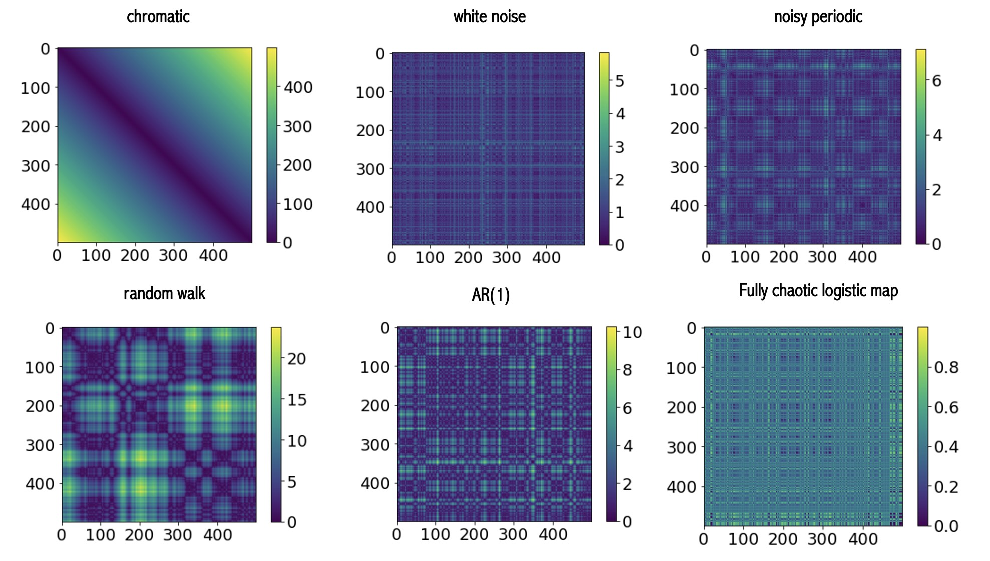
Figure 1: One-dimensional validation set. Distance matrices from one-dimensional trajectories of different complexity, used to provide a preliminary validation of the methods.

3.1 Preliminary validation of complex scalar time series

To validate the methods, we generate time series $\{x_{t}\}_{t=1}^{T}$ from a variety of synthetic, one-dimensional processes with different levels of complexity. In each case, we extract the distance matrix ${\cal D}=\{d_{ij}\};\ d_{ij}=|x_{i}-x_{j}|$ and subsequently build the scalar embedding procedures that yield the different functions $\Phi(\cdot)$ so that the embedded scalar signal is $(z_{t})_{t=1}^{T}$, where $z_{t}=\Phi(x_{t})$. Since the original signal is actually one-dimensional, we assess the validity of the framework by scatter plotting $z_{t}$ vs $x_{t}$ and computing two different correlation coefficients: Pearson’s $r$, and Spearman’s $\rho$. The list of synthetic processes include: (i) a chromatic process $x_{t}=t$, (ii) white Gaussian noise $x_{t}=\xi$, $\xi\sim N(0,1)$, (iii) a noisy periodic signal $x_{t}=\cos(2\pi t/P)+\xi$ of period $P=100$, where $\xi\sim\mathcal{N}(0,\sigma)$ is an extrinsic noise polluting the periodic signal, (iv) a Gaussian random walk $x_{t+1}=x_{t}+\xi$, $\xi\sim\mathcal{N}(0,1)$, (v) an autorreggressive process of order 1 $x_{t+1}=0.7x_{t}+\xi$, $\xi\sim\mathcal{N}(0,1)$, and (vi) a chaotic process generated by a fully chaotic logistic map $x_{t+1}=4x_{t}(1-x_{t})$. In every case we generate a time series of $T=500$ points from these processes. The distance matrices are reported in Fig.1 for illustration.

The distance matrices $\cal D$ are reported in Fig. 1. After building the different scalar embeddings, we have observed that the method based on PCA embedding is systematically successful, as shown by a perfect matching ($r=1$) between the original signal $\{x_{t}\}$ and the embedded signal $\{z_{t}\}$ for all the six time series, implying a perfectly linear relationship $z_{t}=\Phi(x_{t})=\alpha x_{t}$, for some $\alpha\neq 0$. Anecdotically, the explained variance associated to the first principal component hovers around $90\%$ for all six time series. Similar results hold for the method based on classical-MDS. The method based on using a PCA projection is also successful, albeit the scatter plot between $\{x_{t}\}$ and $\{z_{t}\}$ is not a straight line, but rather has a curved shape (with small curvature, so $r<1$ but it is very close to 1) and $\rho=1$. Finally, the method based on using metric-MDS suffers from the problem of observing the onset of what we call “antiphases” in the signal: time points $t$ where, instead of having the correct assignment $z_{t}=\alpha x_{t}$, the embedding provides a sign flipping $z_{t}=-\alpha x_{t}$ (see Fig. 9 for an illustration). The frequency of these undesired antiphases is usually between $1\%$ and $15\%$. These antiphases are clearly observable when the signals are smooth, but it is less evident otherwise. Additionally, these antiphases can break the temporal structure of the embedding, as we will show below. Removing these artifacts is relatively easy in the most simple case where when there is an available ground truth (see Appendix). In general, the best one can do is to assume that the embedding is smooth and flip the sign of the points that violate such assumption, but such smoothness assumption does not necessarily hold. All in all, these issues already makes the strategy based on metric-MDS less useful than the other three.

3.2 Synthetic network trajectories

In the preceding subsection we have validated our methods in the easier case when the original signal is already a scalar time series. We now proceed to analyze synthetic network trajectories of different garment. For simplicity, we make use of the Euclidean norm and, accordingly, the distance $d({\bf A},{\bf A}^{\prime})$ between two network snapshots with adjacency matrices ${\bf A}=\{A_{ij}\}$ and ${\bf A}^{\prime}=\{A^{\prime}_{ij}\}$ is defined as

$$d({\bf A},{\bf A}^{\prime})=\sqrt{\frac{1}{N^{2}}\sum_{i,j=1}^{N}(A_{ij}-A^{\prime}_{ij})^{2}}$$ (12)

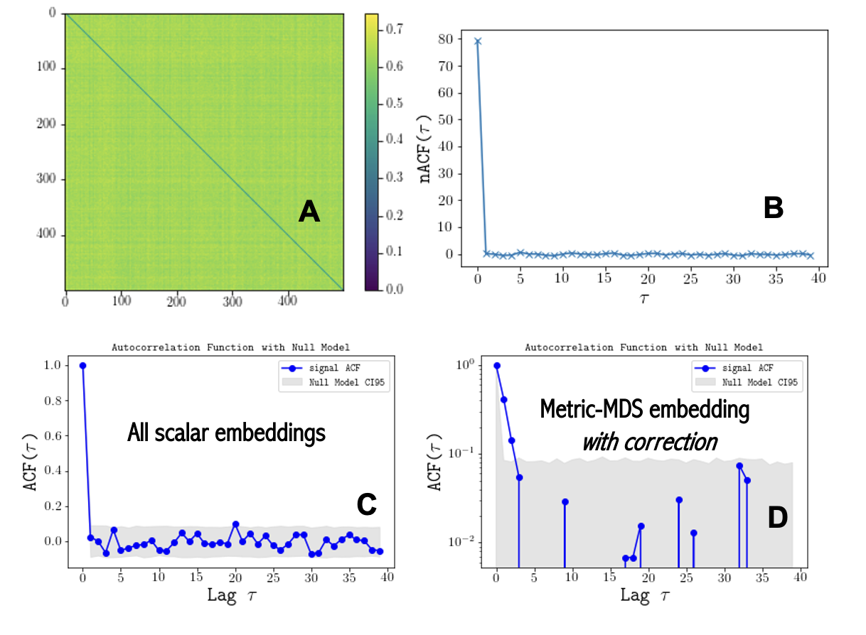
Figure 2: Autocorrelation analysis of white network trajectories and its embeddings. (A) Distance matrix of a network trajectory of $T=500$ snapshots, where each snapshot is an Erdős-Rényi graph of $N=20$ nodes sampled from $\mathscr{G}(20,0.3)$. (B) Network Autocorrelation Function $\text{nACF}(\tau)$ estimated from the network trajectory, showing the characteristic Dirac-delta shape of uncorrelated signals. (C) Scalar autocorrelation function $\text{ACF}(\tau)$ (alongside a $95\%$ confidence interval of a null model where the one-dimensional signal was shuffled $10^{3}$ times) associated to the PCA-embedding, correctly capturing the uncorrelated nature of the network trajectory. All four embeddings display a similar $\text{ACF}(\tau)$ as the one displayed in this panel. (D) Scalar autocorrelation function $\text{ACF}(\tau)$ of the scalar time series $(z_{t})_{t=1}^{500}$ obtained via metric-MDS embedding, after (wrongly) applying the phase correction post-processing (see Appendix). This postprocessing introduces a spurious short memory artifact, as highlighted by the fact that $\text{ACF}(\tau<4)$ appears as statistically significant.

3.2.1 White network trajectories

We start by the simplest network trajectory: one emulating an uncorrelated stochastic process in graph space with a Dirac delta-shaped autocorrelation function. To do that [18], the network trajectory $\cal S$ is built by sampling a total of $T$ Erdős-Rényi graphs from $\mathscr{G}(N,p)$. For illustration, in Fig. 2(A) we show the resulting distance matrix when $T=500$, $N=20$ and $p=0.3$. Figure 2(B) reports the network autocorrelation function, that adequately captures the expected shape (note that $\text{nACF}(0)\neq 1$ as it is not normalized). The scalar embeddings produced by all four strategies yield the correct scalar autocorrelation function (see Fig. 2(C)). Incidentally, observe that in this uncorrelated case the onset of antiphases in the metric-MDS case do not break down the statistical properties of the signal –as the signal remains uncorrelated–, but precisely because of the non-smooth nature of this signal, applying an antiphase correction (which is based on assuming smoothness in the embedding, see Appendix for details) introduces spurious correlations in the metric-MDS embedding, as shown in panel (D) of the figure.

3.2.2 Pulsating network trajectories: the scalar embedding as a noise filter

As a second step, we consider a temporal network model where the weight of each link in the network independently evolves according to the following dynamics: $A_{ij}(t)=\cos(2\pi t/P)+\xi,$ where $P$ is the period of the periodic part of the dynamics and $\xi\sim\mathcal{N}(0,\sigma)$ is an extrinsic noise polluting each link in the network in an uncorrelated way. The periodic component of the individual link dynamics makes the network to ‘pulsate’. Observe that the standard deviation of the noise, $\sigma$, modulates the signal-to-noise ratio (SNR), which goes to zero as $\sigma$ increases as $1/\sigma^{2}$. Here we consider two cases: $\sigma=1$ (where the characterization of periodicity at the link level is still possible although the detection is not fully trivial) and $\sigma=4$ (where there is virtually no trace of the periodic component at the link level, and the link dynamics appears as white noise).

Figure 3: Noisy pulsating network trajectories. We generate noisy pulsating temporal networks, where each link consists in a sinusoidal dynamics polluted with extrinsic Gaussian noise of standard deviation $\sigma$. The left panels display the distance matrix between network snapshots, for two cases: $\sigma=1$ and $\sigma=4$. The middle panels display the time series of an individual link, showing that whereas for the case $\sigma=1$ the individual links still show some (noisy) periodicity, for $\sigma=4$ any sign of periodicity has been washed off by the noise. The right panels display the scalar embedding of the full network trajectory, using two types of embedding strategies: PCA-embedding and classical-MDS, respectively (for readability we only depict the embedding provided by the PCA-embedding and classical-MDS strategies, but results offered by PCA-projection, are similar, and all three are similar for both levels of noise $\sigma$). The three strategies are capable to capture the periodic nature of the network trajectory even when the individual link dynamics are essentially indistinguishable from noise.

For each case, we generate a pulsating network trajectory of $T=10^{3}$ snapshots (where each snapshot has $N=20$ nodes), compute the distance matrix on the network trajectory, and perform the battery of scalar embeddings. We summarise results in Fig. 3. The middle panels display the time series of an individual link, certifying that for $\sigma=1$ the individual links still show some (noisy) periodicity and for $\sigma=4$ any sign of periodicity has been washed off by the noise. The right panels display the scalar embedding of the full network trajectory. For simplicity, we just show two types of embedding strategies, via PCA and classical-MDS respectively (the embedding based on metric-MDS has poorer performance, as expected). Interestingly, not only in the $\sigma=1$ but also for $\sigma=4$, the scalar embeddings clearly enhance the periodic backbone of the network dynamics. The explained variance of the first principal component drops from $88\%$ for $\sigma=1$ to about $32\%$ for $\sigma=4$. Remind that for $T=10^{3}$, full reconstruction requires $10^{3}$ principal components, so the drop in explained variance remains very low).
Overall, results suggest that the scalar embeddings induced by both PCA and classic-MDS strategies are capable of inheriting the pulsating character of the temporal network and filtering out noise, thus enhancing the signal-to-noise ratio.

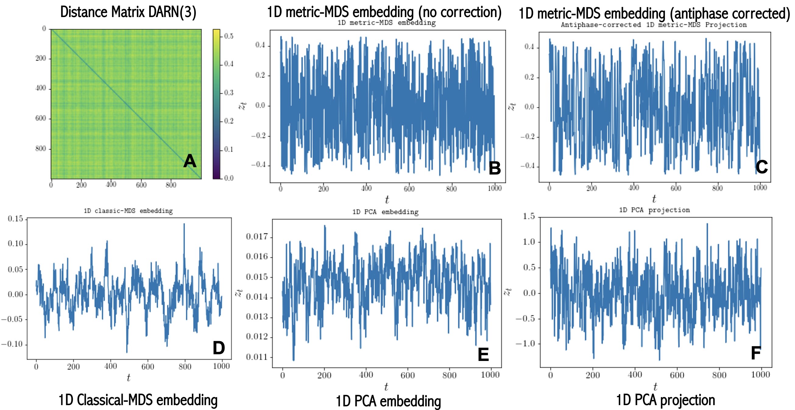
Figure 4: Scalar embedding of DARN(p) network trajectories. Scalar embedding of a correlated temporal network trajectory of $T=10^{3}$ network snapshots generated by a DARN(3) model with parameters $(q,y)=(0.6,0.1)$. (A) Distance matrix between network snapshots, based on Eq.12. Panels (B)–(F) report the one-dimensional (scalar) embedding $(z_{t})_{t=1}^{T},z_{t}\in\mathbb{R}$ of the network trajectory, based on different strategies: (B) Metric-MDS embedding (raw embedding), (C) like (B), but after antiphase correction based on smoothness criterion (about 15% of the datapoints are detected as antiphases and their sign flipped), (D) obtained via classical-MDS embedding, (E) obtained via PCA-embedding, (F) obtained via PCA-projecting.

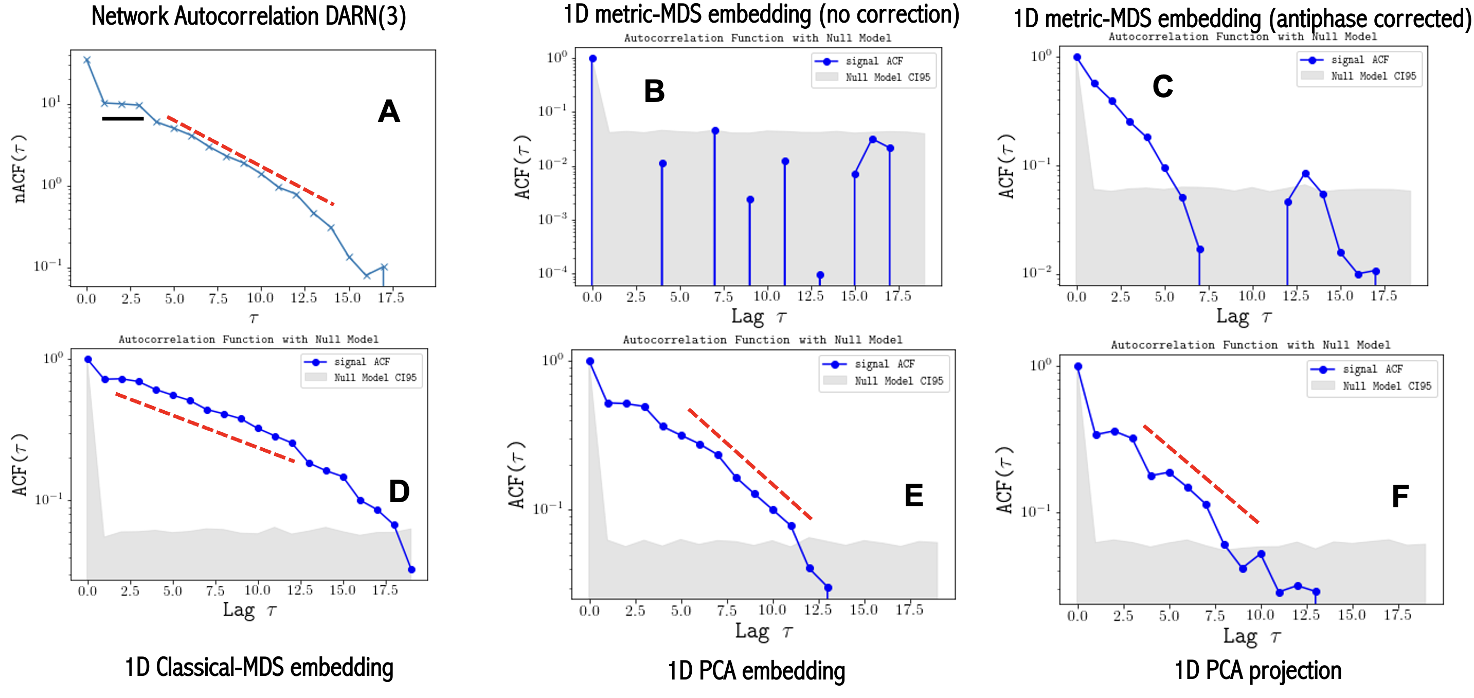
Figure 5: Autocorrelation analysis of DARN(p) network trajectories and its embeddings. (A) Semi-log plot of the Network Autocorrelation Function $\text{nACF}(\tau)$ estimated from the network trajectory $(G_{t})_{t=1}^{1000}$, where each snapshot is a network of 20 nodes) generated by the DARN(3) model reported in Fig.4. The network trajectory has memory order $p=3$, and thus we have $\text{nACF}(1)=\text{nACF}(2)=\text{nACF}(3)$, followed by an exponentially decaying tail for $\tau>p$, as indicated by the dashed lines. Panels (B)–(F) report a semi-log plot of the scalar autocorrelation function $\text{ACF}(\tau)$ of the scalar time series $(z_{t})_{t=1}^{2000}$ (alongside a gray area reporting the $95\%$ confidence interval of a null model which consists in computing such scalar autocorrelation function in an ensemble of $10^{3}$ times shuffled signals). Each panel reports results for the different scalar embeddings of Fig.4: (B) obtained via 1D metric-MDS embedding (raw embedding), (C) like (B), but after antiphase correction based on smoothness criterion, (D) obtained classical-MDS embedding, (E) obtained via PCA-embedding, (F) obtained via PCA-projection. Results further certify that metric-MDS embedding is contaminated with signal antiphases that breaks down linear correlations in the embedding. This correlation structure is only partially recovered after antiphase correction. Scalar embeddings from both classical-MDS and PCA-based methods seem to better capture the autocorrelation function, with a specially good performance by the PCA-embedding strategy.

3.2.3 Network trajectories with memory: DARN(p)

Moving on, we now consider a model that generates temporal network trajectories with memory: the Discrete Autorregressive Network model DARN(p) [17, 24, 18]. In this model, the dynamics of each link $\ell_{t}$ is constructed independently, such that with probability $q$, $\ell_{t+1}$ samples uniformly from its past $p$ states, and with probability $(1-q)$, it assigns a Bernoulli trial with probability $y$. In other words, when the link update is random, we flip a biased coin and assign the entry $1$ (link present) with probability $y$ and the entry $0$ (link absent) with probability $1-y$).
Such process generates a non-Markovian network trajectory with memory order $p$. As ground truth, we use the network autocorrelation function $\text{nACF}(\tau)$, which for DARN($p$) processes has a constant value for lags $\tau\leq p$ and an exponentially decaying curve for larger lags $\tau>p$, against which we will compare the (scalar) autocorrelation function of the scalar embedding.

As a validation, we set $p=3$ and proceed to generate a network trajectory of $T=10^{3}$ snapshots of a DARN(3) model, where each snapshot has $N=20$ nodes and the model parameters are $(q,y)=(0.6,0.1)$. In Fig.4(A) we plot a heatmap of the distance matrix ${\cal D}$ constructed from the network trajectory. Figure 5(A) displays the network autocorrelation function of this network trajectory, displaying the abovementioned characteristic features of DARN(p) models. The different scalar embeddings are reported in panels (B-F) of Fig. 4, namely scalar embeddings based on: metric-MDS (B), metric-MDS after correcting antiphases (C), classical-MDS (D), PCA-embedding (E), and PCA-projection (F). Their respective (scalar) autocorrelation functions are reported in panels (B-F) of Fig. 5. From these results we can conclude that (i) antiphases emerging in metric-MDS embedding break down the temporal correlations of the scalar embedding and thus this method is not suitable, (ii) the fingerprints of the network autocorrelation function are approximately inherited by the rest of the methods, with a specially good performance found in the PCA-embedding (panel E).

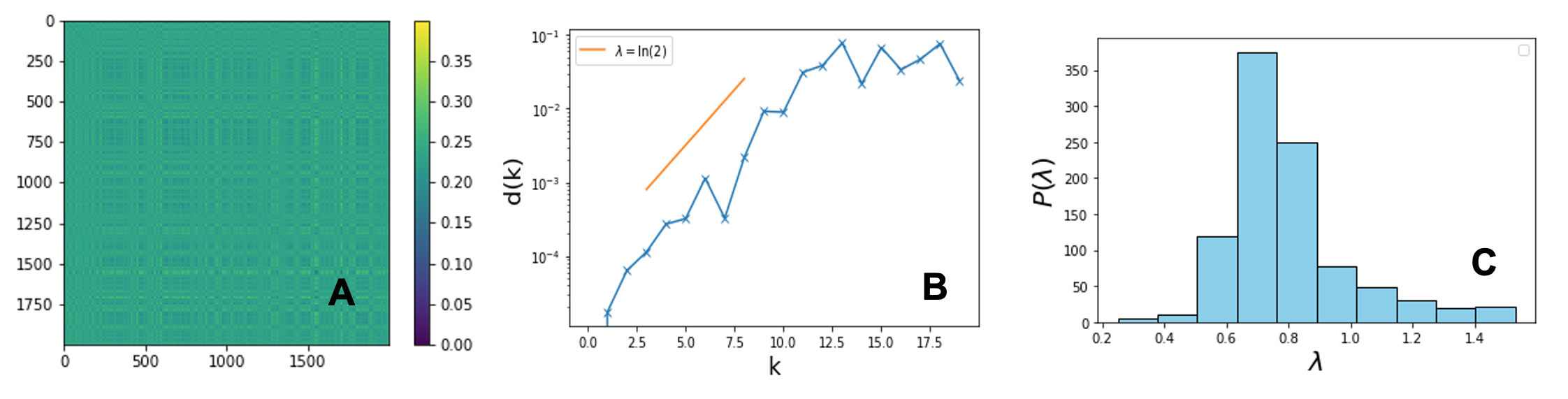
Figure 6: Scalar embedding of a chaotic network trajectory. (A) Distance matrix between network snapshots, for a chaotic network trajectory of $T=2000$ snapshots (where each snapshot has $N=500$ nodes) generated via the dictionary trick, based on a fully chaotic logistic map with theoretical largest Lyapunov exponent $\lambda=\ln 2$. (B) Semi-log plot of the distance $d(k)=|z_{u+k}-z_{v+k}|$ between a pair of initially close points $z_{u}$, $z_{v}$ in the scalar embedding, with $|z_{u}-z_{v}|<10^{-4}$. The distance $d(k)$ increases exponentially (until saturation) with a characteristic exponent close to $\ln 2$. (C) Histogram of characteristic exponents obtained by repeating the procedure in panel (B) for a total of $10^{3}$ initial conditions, bootstrapped from the scalar embedding. The average of the distribution is close to $\ln 2$.

3.2.4 Chaotic network trajectories: the dictionary trick

To round off the theoretical validation, here we illustrate the ability of the scalar embeddings to inherit chaotic properties. To build a chaotic network trajectory, we resort to the so-called dictionary trick [18, 22]. This is a method to generate temporal networks with the same dynamical properties of one-dimensional maps. We initially consider a one-dimensional dynamics generated by the fully chaotic logistic map $x_{t+1}=4x_{t}(1-x_{t})$. This is an interval map $x\in[0,1]$, so the algorithm proceeds by generating a time series $(x_{t})_{t=1}^{T}$, and symbolising the signal after homogeneously partitioning the interval $[0,1]$ into $Q$ equally-sized cells. In parallel, we construct a network dictionary of $Q$ snapshots $\{G[q]\}_{q=1}^{Q}$ (observe that this is a set of networks, not a temporal network). This dictionary is generated sequentially: starting from an initial (e.g. Erdős-Rényi) network of $N$ nodes $G[1]$, in each step of the process a unique link rewiring is performed. Iterating such process builds $G[2]$, $G[3]$, etc. Such rewiring needs to follow two strict rules: (i) one cannot select a link which had already been inserted from a previous rewiring, and (ii) the new link cannot be inserted in a place which previously had a link that had eventually been rewired. By following these two rules, the sequence of generated networks is metrical: any two $G[s]$ and $G[t]$ are precisely $t-s$ rewirings apart, so ${\left\|G[s]-G[t]\right\|}=|t-s|$. Once the dictionary is built, each cell of the interval $[0,1]$ is matched with a network of the dictionary, so that the first cell is assigned $G[1]$, the second cell is assigned $G[2]$, and so on. Finally, each point of the time series $x_{t}$ is mapped to a network which we label $G_{t}$, thereby constructing a temporal network $(G_{t})_{t=1}^{T}$ with the same dynamical properties of $(x_{t})_{t=1}^{T}$.

We have applied this procedure with $Q=10^{4}$, and constructed a network trajectory of $T=2000$ snapshots, where each snapshot is a network with $N=500$ nodes. In Fig.6(A), we show the distance matrix of the network trajectory, displaying an apparent uncorrelated structure. After computing its scalar embedding $(z_{t})_{t=1}^{T}$ (based for illustration in the PCA-embedding strategy), Fig. 6(B) displays a semi-log plot of the distance $d(k)=|z_{u+k}-z_{v+k}|$, where $z_{u}$ and $z_{v}$ are two points which are close in the embedding space i.e. $|z_{u}-z_{v}|<\epsilon=10^{-4}$ –these are akin to recurrences of the trajectory, as in Wolf’s method [22, 38]–. The orange solid line depicts an exponential expansion with slope $\lambda=\ln 2$, the Lyapunov exponent of the fully chaotic logistic map. These results suggest that the scalar embedding has inherited the chaotic properties of the network trajectory. Indeed, we typically observe exponential expansion of nearby trajectories for almost all initial conditions. Note that here we used the PCA-embedding strategy, but the other three embedding strategies work reasonably well, with the caveat that the metric-MDS one requires antiphase correction. Figure 6(C) displays the distribution $P(\lambda)$ obtained when bootstrapping a total of $10^{3}$ initial conditions from the scalar embedding (as in Wolf’s method). The average of the distribution is the theoretical analogue of the network Maximum Lyapunov Exponent [22] in the scalar embedding, indeed finding it to be close to $\ln 2$.

3.3 Empirical network trajectories

We finally illustrate the performance of the scalar embedding in two real (empirical) temporal network trajectories. We have concentrated in the scalar embedding obtained via the PCA-embedding strategy, as it showed a consistently good performance in the previous section.

3.3.1 Emails

In Fig. 7 we present results on an empirical email network trajectory that was previously identified as having a periodic backbone [18]. This is a directed temporal network of emails in the 2016 Democratic National Comittee (DNC). In this network, each node represents a person, and directed edges indicate that one person has sent an email to another. Because an email can be sent to multiple recipients, each email is represented by several edges. We have aggregated into the same network snapshot all timestamped edges belonging within a time window of 24 hours. The resulting network trajectory is highly non-stationary, with an initial period of almost no activity. Accordingly, we focus only in a period of the last 30 days (one-month activity, i.e. 30 snapshots), where there was a substantial email exchange. Results in Fig.7 confirm that the scalar embedding of this network trajectory captures the periodic backbone. The periodic fingerprint appears to be enhanced in the scalar autocorelation function (see Fig. 7(C)) with respect to the nACF case (Fig. 7(C)) . This result supports that the scalar embedding acts as a filter that enhances the signal-to-noise ratio, in agreement with what was observed for synthetic noisy periodic network trajectories.

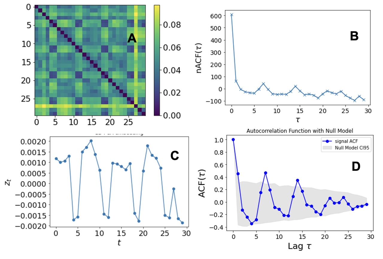
Figure 7: Embedding of email network trajectory from the democratic national committee. (A) Distance matrix between network snapshots, for a trajectory of $T=30$ snapshots (one month). Each snapshot aggregates the email activity over a total of one day, between $1800$ individuals. $\tau$ scale is in days. (B) Network autocorrelation function $\text{nACF}(\tau)$ estimated from the network trajectory. The function displays a subtle periodic behavior, with period $\tau=7$ days (weekly periodicity). (C) Scalar embedding of the network trajectory (PCA-embedding). (D) Scalar autocorrelation function $\text{ACF}(\tau)$, where the periodic backbone is clearly enhanced.

3.3.2 Sociopatterns

We have further explored the scalar embedding of empirical temporal networks obtained from the Sociopatterns project. In Fig.8 we show the results applied to a primary school temporal network trajectory. This network trajectory has $T=1300$ snapshots (based on the aggregation window, roughly equivalent to 8.5 hours), where each snapshot has $N=243$ nodes which correspond to students in a primary school, and links model proximity-based interaction [40]. This is a subset of the original temporal network, and we selected only one day of data to remove any source of daily periodicity. Our results show that the interaction activity strongly fluctuates throughout the day (Fig. 8(A)) and that the network trajectory displays memory, with a characteristic timescale of about 47 minutes, as found with the network autocorrelation function (Fig. 8(C)). This characteristic timescale is similar to the typical duration of a lecture. The scalar embedding based on the PCA-embedding strategy (Fig. 8(D)) almost perfectly retrieves the dynamics (explained variance of the first principal component is over $92\%$), and its autocorrelation function also displays decaying memory with the same characteristic timescale of 47 minutes (Fig. 8(E)). Now, since the number of links strongly fluctuates over time –tracking different levels of activity in the system–, we wonder whether the network dynamics is primarily influenced by such effective one-dimensional degree of freedom. To remove such variability –and thus make the task of retrieving dynamics from the scalar embedding substantially more challenging–, we now pollute each snapshot with different amounts of noise (i.e. adding links at random), such that the number of active links across snapshots is the same for all the snapshots, see (Fig. 8(F)). This is akin to superposing a non-constant amount of extrinsic noise. Interestingly, the memory structure detected by the network autocorrelation –as well its the characteristic timescale– is conserved after this drastic contamination (Fig. 8(H)). This means that the memory pattern cannot be attributed to the link density fluctuations. As for the scalar embedding, the explained variance of the first principal component decreases but remains substantial (over $17\%$ in a system of 1300 principal components). The autocorrelation function still displays decaying memory, although the characteristic timescale is larger.

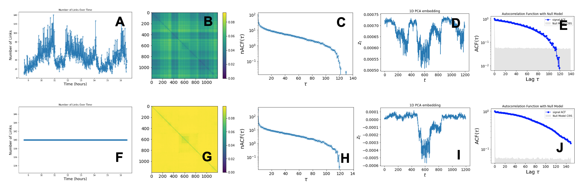
Figure 8: Embedding of primary school temporal network trajectory. The network trajectory of $T=1300$ snapshots (roughly equivalent to 8.5 hours of intraday activity in a primary school), where each snapshot has $N=243$ nodes (students) and links model proximity-based interactions among students. This is a subset of the original temporal network, where only one day of activity is selected to remove any source of daily periodicity. (A) Time series of the number of links of each network snapshot, showing a clear heterogeneous interaction intensity from 9AM to 4PM. (B) The distance matrix of the network trajectory. (C) Semi-log plot of the network autocorrelation function $\text{nACF}(\tau)$, showing a decaying shape –i.e. memory– with a characteristic timescale of $\tau=120$ (roughly equivalent to a characteristic time of 47 minutes). (D) Scalar embedding $z_{t}$, based on the PCA-embedding strategy. The explained variance by the first principal component is $92\%$. (E) Semi-log plot of the scalar autocorrelation function $\text{ACF}(\tau)$ of the scalar embedding, showing hints of memory with a characteristic timescale of $\tau=120$ (roughly 47 minutes), equal to the one detected by the network autocorrelation function. (F) Same as (A), after having polluted the network trajectory with noise of varying intensity, such that each network snapshot has a fixed number of links. This removes the source of dynamics based on number of links, and in principle makes the embedding much more challenging. (G-J) Same as (B-E), for the contaminated network trajectory. Despite the substantial amount of time-varying noise contamination, the network autocorrelation function shows the same shape –an exponential decay of correlations with a cutoff at $\tau=120$ (roughly equivalent to a characteristic time of 47 minutes)–. The explained variance by the first principal component drops to $17\%$ The scalar autocorrelation function $\text{ACF}(\tau)$ still shows hints of memory although with a larger characteristic scale.

4 Discussion

In this work we have explored the performance of four similar strategies –all based on leveraging linear dimensionality reduction techniques– to extract a scalar embedding (i.e. one-dimensional time series) out of a temporal network trajectory. The common insight underpinning such approaches is that the key information which is relevant for capturing the intrinsic dynamics of the temporal network trajectory lies in the relative distance between network snapshots, rather than specific structure within each snapshot, i.e. inter-snapshot information, rather than intra-snapshot one. We have validated the approaches by constructing several synthetic models of network trajectories with different types of dynamics, finding that their scalar embeddings adequately inherit the planted dynamical fingerprints. We have also provided some evidence supporting that the scalar embedding behaves as a filter that enhances the signal-to-noise ratio of the original network trajectory. The analysis of two empirical network trajectories further confirms the applicability of the method in realistic, high dimensional scenarios.

Out of the four strategies under analysis, embedding and projection based on PCA and classical-MDS work substantially better than the one based on metric-MDS. There is no clearly superior method among the three successful ones (i.e., PCA-projection, PCA-embedding and classical-MDS), as some work slightly better than others in different cases. However, PCA’s explained variance of the first principal component can be used as a quantification of how much information is discarded in the dimensionality reduction, and this might give these strategies an interpretability advantage. Observe that despite the severe dimensionality reduction, the scalar embedding captures substantial and nontrivial dynamical properties of the original network trajectory. All in all, we thus consider the conceptual approach advanced here to be promising and offers an avenue for making time series analysis of temporal networks, with high applicability across the disciplines.

Let us now outline some limitations and open questions for further work. First, this paper proposes a proof of concept, focusing on scalar embeddings. In this sense, the method can be straightforwardly generalized to dimensions larger than one –if and when needed– along the lines described in Section 2. Second, computational efficiency of the method could also be improved in future work, e.g. by considering online versions of the embedding algorithms. Third, as a proof of concept we used an Euclidean norm to assess the distance between two network snapshots, but other choices are also possible. Fourth, on relation to the feature matix, in this work we have treated as ‘equally important features’ all the relative distances of a snapshot to any other snapshot. This assumption is perhaps too strict, as one can argue that the relative distance between closer snapshots (in time) is a more important feature than the relative distance between snapshot that are very far apart in time. Accordingly, a possible improvement for future work could define some ‘weight decay’ (e.g. a kernel) between snapshots based on how close the snapshots are in time. This kernel could, in turn, boost the computational efficiency of the whole methodology. Fifth, it would be interesting to consider other dynamical quantifiers beyond linear correlations or dynamical stability. Sixth, extracting faithful scalar embeddings of temporal networks would enable to directly assess the similarity among different network trajectories, a topic of recent interest [41]. Finally, note that the dimensionality reduction approaches considered here are inherently linear. In this sense, further work should assess the viability of nonlinear techniques, ranging from classical nonlinear dimensionality reduction methods to recent machine learning solutions.

Appendix: Spontaneous sign flipping detection

The scalar embeddings $z_{t}$ obtained via metric-MDS sometimes appear to suffer from rando, unexpected sign flips $z\to-z$ for some time values $t$. We call these sign flips antiphases, alluding to the fact that $e^{i\pi}=-1$: sign flip is equivalent to a rotation of $\pi$. In Fig. 9 we illustrate this phenomenon in a controlled scenario where we use the metric-MDS strategy to extract the scalar embedding $z_{t}=\Phi(x_{t})$, where $x_{t}$ is the result of one-dimensional random walk $x_{t+1}=x_{t}+\xi$. Panel (B) displays the one-dimensional original time series $(x_{t})_{t=1}^{500}$. For comparison, Panel (C) displays a correct scalar embedding via classical-MDS. Panel (E) displays the scalar embedding obtained via metric-MDS. Panel (D) depicts a scatter plot between $z_{t}$ (as obtained via metric-MDS) and $x_{t}$, detecting the values $x_{t}$ for which there seems to be a sign flip. These points can affect the subsequent statistical analysis of the embedded trajectory, and thus need to be detected and corrected before any analysis. To do that, we introduce two simple techniques, depending on whether we have access or not to a ground true scalar trajectory $(x_{t})$. If we have access to the ground true one-dimensional signal, the antiphase correction is a simple iterative method whereby:

1. Initially, we consider a scatter plot $z_{t}$ vs $x_{t}$, and we fit a straight line. The quality of the fit is ruined by the points with spontaneous sign flip: correcting these signs will then yield to an improved fit. Therefore:

2. All the points $\{{x_{t}}\}$ considered outliers of the linear fit (residual error larger than a certain threshold) are flipped ${x_{t}}\to-{x_{t}}$. The changes are accepted if the Pearson’s $R^{2}$ of the scatter plot does not decrease.

3. Steps (1) and (2) are repeated until convergence (i.e. no more outliers are detected or the flip does not increase $R^{2}$).

This technique is applied in Fig.9(F). Unfortunately, this method cannot be applied when we do not have access to $\{x_{t}\}$ (e.g., for temporal networks). In the latter case, we can always implement an antiphase correction that relies on a property of smoothness: if $z_{t}$ is not in antiphase , and if the magnitude of $z_{t+1}$ (i.e. $|z_{t+1}|$) is sufficiently close to $z_{t}$ but its sign is flipped, then it is highly likely that an antiphase took place at $z_{t+1}$, and we perform the flip $z_{t+1}\to-z_{t+1}$. Note, however, that the validity of this method relies on the smoothness assumption. This assumption does not hold e.g. in very network trajectories.

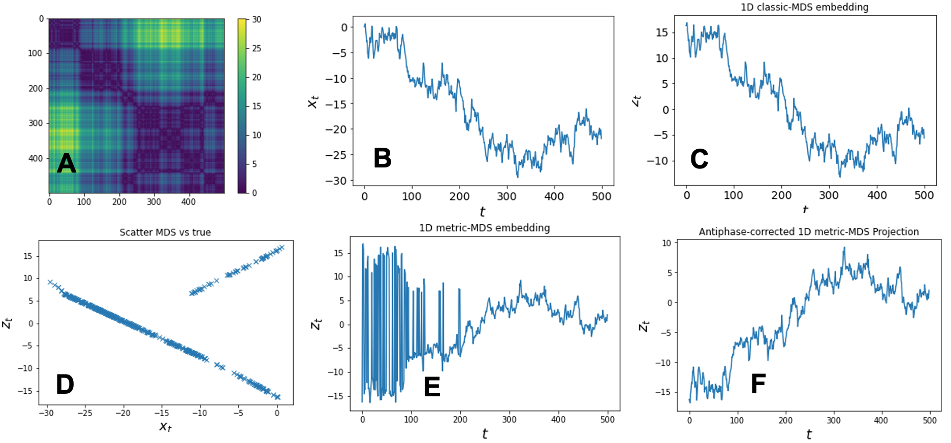
Figure 9: Onset and correction of antiphases. (A) Distance matrix of a toy one-dimensional random walk trajectory $x_{t+1}=x_{t}+\xi$. (B) Random walk trajectory $(x_{t})_{t=1}^{500}$. (C) Example of scalar embedding $z_{t}$ that works correctly. We used the classic-MDS one, but the result is similar with the PCA-based ones. (D-E) Illustration of the onset of antiphases $z_{t}\to-z_{t}$ that emerge for some time values when using metric-MDS based embedding. (D) Scatter plot $z_{t}$ vs $x_{t}$, where we observe that several points have a $z_{t}\to-z_{t}$ flip.(E) metric-MDS scalar embedding, where we clearly see the position of the antiphases. (F) Antiphase-corrected embedding.

Acknowledgments – LL and LAF acknowledge partial support from projects DYNDEEP (EUR2021- 122007) MISLAND (PID2020-114324GB-C22) and Maria de Maeztu (CEX2021-001164-M) funded by the MICIU/AEI/10.13039/501100011033. NM acknowledges partial support from the National Science Foundation (grant no. 2052720), the Japan Science and Technology Agency (JST) Moonshot R&D (grant no. JPMJMS2021), and JSPS KAKENHI (grant nos. JP 23H03414, 24K14840, and 24K030130).

Code availability – All codes will be available upon publication at https://github.com/lucaslacasa

References

- [1] Vito Latora, Vincenzo Nicosia, and Giovanni Russo. Complex networks: principles, methods and applications. Cambridge University Press, 2017.
- [2] Mark Newman. Networks. Oxford university press, 2018.
- [3] Naoki Masuda and Renaud Lambiotte. A Guide to Temporal Networks. 2016.
- [4] Petter Holme and Jari Saramäki. Temporal networks. Physics Reports, 519(3):97–125, October 2012.
- [5] Petter Holme. Modern temporal network theory: a colloquium. The European Physical Journal B, 88(9), September 2015.
- [6] Petter Holme and Jari Saramäki. Temporal network theory, volume 2. Springer, 2019.
- [7] Naoki Masuda, Konstantin Klemm, and Víctor M Eguíluz. Temporal networks: slowing down diffusion by long lasting interactions. Physical Review Letters, 111(18):188701, 2013.
- [8] Jean-Charles Delvenne, Renaud Lambiotte, and Luis EC Rocha. Diffusion on networked systems is a question of time or structure. Nature communications, 6(1):7366, 2015.
- [9] Ingo Scholtes, Nicolas Wider, René Pfitzner, Antonios Garas, Claudio J Tessone, and Frank Schweitzer. Causality-driven slow-down and speed-up of diffusion in non-markovian temporal networks. Nature communications, 5(1):5024, 2014.
- [10] M. Starnini, A. Baronchelli, and R. Pastor-Satorras. Modeling human dynamics of face-to-face interaction networks. Physical Review Letters, 110:168701, Apr 2013.
- [11] Piero Mazzarisi, Paolo Barucca, Fabrizio Lillo, and Daniele Tantari. A dynamic network model with persistent links and node-specific latent variables, with an application to the interbank market. European Journal of Operational Research, 281(1):50–65, 2020.
- [12] Takayuki Hiraoka and Hang-Hyun Jo. Correlated bursts in temporal networks slow down spreading. Scientific reports, 8(1):15321, 2018.
- [13] P Van Mieghem and R Van de Bovenkamp. Non-markovian infection spread dramatically alters the susceptible-infected-susceptible epidemic threshold in networks. Physical review letters, 110(10):108701, 2013.
- [14] William Hedley Thompson, Per Brantefors, and Peter Fransson. From static to temporal network theory: Applications to functional brain connectivity. Network Neuroscience, 1(2):69–99, 2017.
- [15] Massimiliano Zanin, Lucas Lacasa, and Miguel Cea. Dynamics in scheduled networks. Chaos: An Interdisciplinary Journal of Nonlinear Science, 19(2), 2009.
- [16] Massimiliano Zanin and Fabrizio Lillo. Modelling the air transport with complex networks: A short review. The European Physical Journal Special Topics, 215(1):5–21, 2013.
- [17] Oliver E Williams, Fabrizio Lillo, and Vito Latora. Effects of memory on spreading processes in non-markovian temporal networks. New Journal of Physics, 21(4):043028, 2019.
- [18] Lucas Lacasa, Jorge P. Rodriguez, and Victor M. Eguiluz. Correlations of network trajectories. Phys. Rev. Res., 4:L042008, Oct 2022.
- [19] Harrison Hartle and Naoki Masuda. Autocorrelation properties of temporal networks governed by dynamic node variables. arXiv preprint arXiv:2408.16270, 2024.
- [20] Francisco Bauzá Mingueza, Mario Floría, Jesús Gómez-Gardeñes, Alex Arenas, and Alessio Cardillo. Characterization of interactions’ persistence in time-varying networks. Scientific Reports, 13(1):765, 2023.
- [21] Elsa Andres, Alain Barrat, and Márton Karsai. Detecting periodic time scales of changes in temporal networks. Journal of Complex Networks, 12(2):cnae004, 2024.
- [22] Annalisa Caligiuri, Victor M. Eguíluz, Leonardo Di Gaetano, Tobias Galla, and Lucas Lacasa. Lyapunov exponents for temporal networks. Phys. Rev. E, 107:044305, Apr 2023.
- [23] Kaloyan Danovski, Miguel C Soriano, and Lucas Lacasa. Dynamical stability and chaos in artificial neural network trajectories along training. Frontiers in Complex Systems, 2:1367957, 2024.
- [24] Oliver E Williams, Lucas Lacasa, Ana P Millán, and Vito Latora. The shape of memory in temporal networks. Nature communications, 13(1):499, 2022.
- [25] Changping Wang, Chaokun Wang, Zheng Wang, Xiaojun Ye, and Philip S. Yu. Edge2vec: Edge-based social network embedding. ACM Trans. Knowl. Discov. Data, 14(4), may 2020.
- [26] Mikhail Belkin and Partha Niyogi. Laplacian eigenmaps and spectral techniques for embedding and clustering. Advances in neural information processing systems, 14, 2001.
- [27] Sam T Roweis and Lawrence K Saul. Nonlinear dimensionality reduction by locally linear embedding. science, 290(5500):2323–2326, 2000.
- [28] Amr Ahmed, Nino Shervashidze, Shravan Narayanamurthy, Vanja Josifovski, and Alexander J Smola. Distributed large-scale natural graph factorization. In Proceedings of the 22nd international conference on World Wide Web, pages 37–48, 2013.
- [29] Palash Goyal and Emilio Ferrara. Graph embedding techniques, applications, and performance: A survey. Knowledge-Based Systems, 151:78–94, 2018.
- [30] Giang Hoang Nguyen, John Boaz Lee, Ryan A. Rossi, Nesreen Ahmed, Eunyee Koh, and Sungchul Kim. Continuous-time dynamic network embeddings. Companion Proceedings of the The Web Conference 2018, 2018.
- [31] Jundong Li, Harsh Dani, Xia Hu, Jiliang Tang, Yi Chang, and Huan Liu. Attributed network embedding for learning in a dynamic environment. In Proceedings of the 2017 ACM on Conference on Information and Knowledge Management, CIKM ’17, page 387–396, New York, NY, USA, 2017. Association for Computing Machinery.
- [32] Chanon Thongprayoon, Lorenzo Livi, and Naoki Masuda. Embedding and trajectories of temporal networks. IEEE Access, 11:41426–41443, 2023.
- [33] Naoki Masuda and Petter Holme. Detecting sequences of system states in temporal networks. Scientific Reports, 9(1), January 2019.
- [34] Chanon Thongprayoon and Naoki Masuda. Online landmark replacement for out-of-sample dimensionality reduction methods. arXiv preprint arXiv:2311.12646, 2023.
- [35] Chanon Thongprayoon and Naoki Masuda. Spline tie-decay temporal networks. arXiv preprint arXiv:2408.11913, 2024.
- [36] Ian T. Jolliffe. Principal Component Analysis. Springer, New York, 2nd edition, 2002.
- [37] Ingwer Borg and Patrick J. F. Groenen. Modern Multidimensional Scaling: Theory and Applications. Springer, New York, 2nd edition, 2005.
- [38] Alan Wolf, Jack B Swift, Harry L Swinney, and John A Vastano. Determining lyapunov exponents from a time series. Physica D: nonlinear phenomena, 16(3):285–317, 1985.
- [39] Ryan Rossi and Nesreen Ahmed. The network data repository with interactive graph analytics and visualization. In Proceedings of the AAAI conference on artificial intelligence, volume 29, 2015.
- [40] Juliette Stehlé, Nicolas Voirin, Alain Barrat, Ciro Cattuto, Lorenzo Isella, Jean-François Pinton, Marco Quaggiotto, Wouter Van den Broeck, Corinne Régis, Bruno Lina, et al. High-resolution measurements of face-to-face contact patterns in a primary school. PloS one, 6(8):e23176, 2011.
- [41] Lorenzo Dall’Amico, Alain Barrat, and Ciro Cattuto. An embedding-based distance for temporal graphs. Nature Communications, 15(1), 2024.