Controlling independently the heading and the position of a Dubins car using Lie brackets
Abstract
In this paper, we give a control approach to follow a trajectory for a Dubins car controlling the heading independently. The difficulty is that the Dubins car should have a heading corresponding to the argument of the vector speed of the vehicle. This non holonomic constraint can be relaxed thanks to a specific control which uses Lie brackets. We will show such a control will allow us, at least from a theoretical point of view, to control independently the moving position of the car and the heading.
1 Introduction
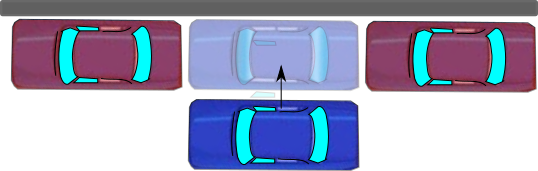
The motivation of Lie brackets for control is illustrated by Figure 1 on the car parking problem. We would like to move the blue car sideway between the two red cars already parked. Moving sideway is not possible, but we can approach this direction using many small forward-backward maneuvers. Building this new sideway direction corresponds to the Lie bracket operator between two dynamics.
The difficulty that we meet when we park a car is that we have two inputs (the acceleration and the steering wheel) whereas we want to control three quantities: two for the position and one for the heading. The goal of this paper is to illustrate how controlling three directions from two actuators can be done using Lie brackets. This will be illustrated on the case of a first order Dubins car and a second order Dubins car [3][11].
2 Control of a driftless system with two inputs
A driftless system is a system of the form
| (1) |
where is the state vector, is the input vector, is a matrix which depends on . If then the evolution of the system stops. Lie brackets are mainly used to control this type of systems. In this section, for simplicity, we consider that , which means that we have two inputs.
2.1 Definition of Lie brackets
Consider two vector fields f and of corresponding to two state equations and . We define the Lie bracket between these two vector fields as
| (2) |
The adjoint notation can be used:
| (3) |
We can check that the set of vector fields equipped with the Lie bracket is a Lie algebra. The proof is not difficult but tedious. As a consequence we have the following Jacobi equality
| (4) |
In this paper, the fact that the set of vector fields equipped with the Lie bracket is a Lie algebra will not be needed.
As an example, consider the two linear vector fields , . We have
| (5) |
2.2 Creating new direction with Lie brackets
Lie brackets are often used to check the local accessibility near driftless states [13] [1]. The accessibility distribution (or Lie ideal) Lie of two vector fields is obtained by taking all vector fields that can be generated using Lie brackets from and [4]. If at a driftless state , Lie spans all directions of , then we can conclude [12]) that the system is locally accessible. Now, Lie brackets can also be used to control driftless systems as shown by the following proposition.
Proposition 1.
Consider the driftless system
| (6) |
Consider the following cyclic sequence:
where is an infinitesimal time period . This periodic sequence will be denoted by
| (7) |
We have:
| (8) |
Proof.
Without loss of generality, the proof will be done for . We shall use the following notations
| (9) |
For a given , and a small we have
| (10) |
with
| (11) |
Taking the cyclic sequence, we have
| (12) |
We get
| (13) |
The sum yields
Now,
Therefore
| (14) |
The same reasoning yields
This result could be obtained directly from (14) by rewriting: . Thus
| (15) |
The consequence is that using the periodic sequence, we are now able to move with respect to the direction . ∎
2.3 Controlling the new direction created by the Lie brackets
In this section, we want to find which periodic sequence we should take in order to follow the field . We will first consider the case and then the case .
We have shown that within a time period of we moved in the direction by . This means that we follow the field which is infinitesimal. Multiplying the cyclic sequence by the scalar amounts to multiplying both by . The field thus becomes . If we want the field , we have to multiply the sequence by . If is negative, we have to change the orientation of the sequence. The cyclic sequence is thus
| (16) |
where changes the orientation of the sequence (clockwise for , counterclockwise for ).
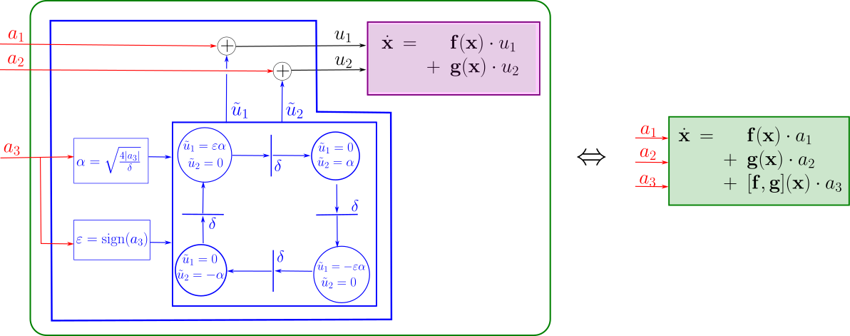
2.4 Controller
In this section, we propose a controller such that closed loop system becomes
where is the new input vector.
If we want to follow the field , we have to take the sequence
| (17) |
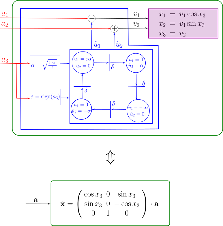
with and As illustrated by Figure 2, we succeeded to create a new input to our system which corresponds to the direction pointed by the Lie bracket. Note that the equivalence given in the figure should be understood as an approximation since is not infinitesimal.
3 Control of the first order Dubins car
3.1 Dubins car
Consider a Dubins car described by the following state equations:
| (18) |
where is the speed of the cart, the rotation rate, its orientation and the coordinates of its center. Using Lie Brackets, we can add a new input to the system, i.e., a new direction of control. We call this vehicle a first order Dubins car, since we control the speed and the rotation rate directly. It will be a second order Dubins car when their derivative will be controlled instead.
If we set , we have
| (19) |
We have
| (20) |
We conclude that we can now move the car laterally.
3.2 Simulation
We propose a simulation (taken from [8] [9]) to check the good behavior of your controller. To do this, take small enough to be consistent with the second order Taylor approximation but large with respect to the sampling time For instance, we may take The initial state vector is taken as .
If we apply the cyclic sequence as a controller, we get
| (21) |
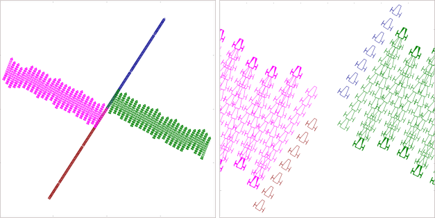
We made 4 simulations for , , and . We took for initial vector , and . We obtained the results depicted on Figure 3. We observe that after each simulation, the distance to the origin is approximately which is consistent we the fact that and have a norm equal to 1. We did not show the simulation for since there no displacement: the car turns on itself.
3.3 Control the cardinal directions
We now propose a controller so that the car follows the cardinal directions, i.e., North, South, East, West. We have
| (22) |
We take to get , where .
For take sequentially the desired directions: , , , We get the results shown on Figure 4.
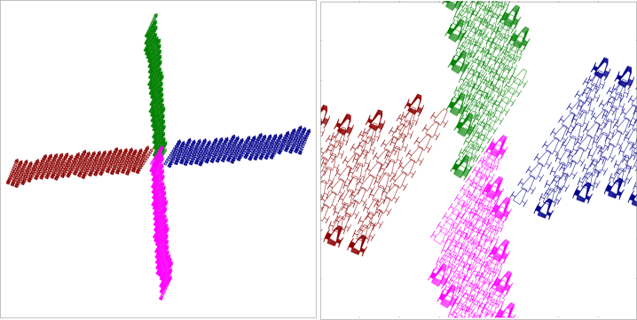
Figure 5 shows the complete controller for our Dubins car to follow a desired pose trajectory . For this, a high gain proportional controller was added. As we will see in the following section, we have a right inverse of the first order Dubins car.

4 Control of the second order Dubins car
4.1 Model
We consider the second order Dubins car given by
| (23) |
or equivalently
| (24) |
The system has a drift which cannot be directly controlled. To control such a system, we can use a backstepping technique by decomposing the system as a sequence of right invertible systems.
4.2 Right inverse
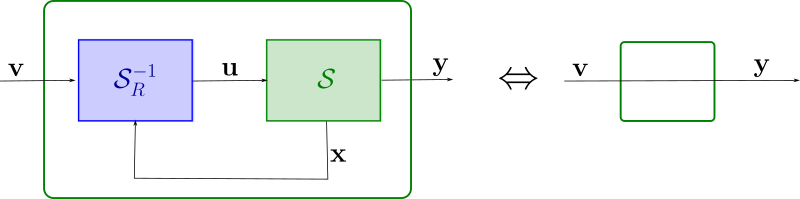
The notion of right invertibility comes from [6] and [2], Section 3.3.3. The notion right invertibility is illustrated by Figure 6 and says that if we put the controller in front of , the effect of will be canceled. Equivalently, we have .
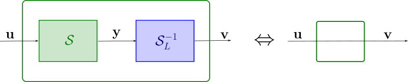
Similarly, the notion left invertibility is illustrated by Figure 7 and says that if we put the system after , the effect of will be canceled, i.e, . This left invertibility corresponds more or less to an observer and will not be used later in this paper.
4.3 Backstepping control of the car
As illustrated by Figure 8, our Dubins car can be decomposed into two systems. Both are right invertible.
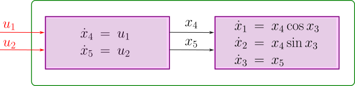
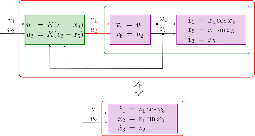
Indeed, the first block of Figure 9, corresponding to two integrators in parallel, can be eliminated by adding a proportional controller with a gain . If is large enough, we can consider that and . We thus get a first order Dubins car.
As seen previously (see Figure 2), the first order Dubins, which is a driftless system with two inputs and three states can be controlled using Lie brackets. As illustrated by Figure 10, the resulting vehicle can be controlled tangentially (i.e., forward and backward), laterally (i.e., left and right), and in orientation, all independently.
As illustrated by Figure 10, using a feedback linearization [14], we can control the car in all directions in the robot frame.
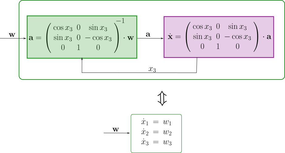
Finally, with a simple proportional control, we can follow any pose trajectory , (see Figure 12), i.e., a trajectory in the world frame, with a heading which can be chosen independently.
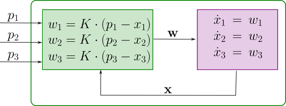
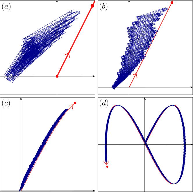
Figure 13 shows the trajectory of the car for the wanted Lissajou trajectory :
| (25) |
and for different periods of time. Subfigure (a) shows the beginning of the mission. We observe that the car maneuvers to have both a heading to East and reach the target point (red). Subfigure (b) shows the mission a few seconds later. The heading is now almost to East, as expected. Subfigures (c) and (d) demonstrate the ability for the Dubins to follows the Lissajou curve, always pointing to East.
5 Conclusion
In control theory [5][7][10][12], when dealing with nonlinear systems, we generally ask to control states variables if we have inputs. Using Lie brackets, we can control more than variables, but the new directions of control only allow infinitesimal displacements in the state space. These displacements can be obtained using infinitesimal cycles created by the Lie brackets. These cycles may be interpreted as an infinitesimal time-division multiplexing (TDM) method, used for transmitting and receiving independent signals over a common signal path by means of synchronized switches.
In this paper, we have illustrated the principle of the approach on a first order and a second order Dubins cars. Using Lie brackets, we have shown that we were able to move a car sideway to make a parking slot, even if sideway motion are very slow.
The source codes of the simulations and a video associated to the experiment are available at
References
- [1] B. d’Andréa Novel. Commande non-linéaire des robots. Hermès, Paris, France, 1988.
- [2] F.J. Doyle and M.A. Henson. Nonlinear Systems Theory. Prentice-Hall, 1997.
- [3] L. E. Dubins. On curves of minimal length with a constraint on average curvature, and with prescribed initial and terminal positions and tangents. American Journal of Mathematics, 79(3):497, jul 1957.
- [4] I. Duleba and W. Khefifi. A lie algebraic method of motion planning for driftless nonholonomic systems. In Krzysztof Kozlowski, editor, Proceedings of the Fifth International Workshop on Robot Motion and Control, RoMoCo 2005, Poznań, Poland, June 23-25, 2005, pages 79–84. IEEE, 2005.
- [5] I. Fantoni and R. Lozano. Non-linear control for underactuated mechanical systems. Springer-Verlag, 2001.
- [6] R. M. Hirschorn. Invertibility of nonlinear control systems. SIAM Journal on Control and Optimization, 17(2):289–297, 1979.
- [7] A. Isidori. Nonlinear Control Systems: An Introduction, 3rd Ed. Springer-Verlag, New-York, 1995.
- [8] L. Jaulin. Mobile Robotics. ISTE editions, 2015.
- [9] L. Jaulin. InMOOC, inertial tools for robotics , www.ensta-bretagne.fr/inmooc/. ENSTA-Bretagne, 2019.
- [10] H.K. Khalil. Nonlinear Systems, Third Edition. Prentice Hall, 2002.
- [11] J. P. Laumond. Feasible trajectories for mobile robots with kinematic and environment constraints. In Proceedings of the International Conference on Intelligent Autonomous Systems, pages 246–354, Amsterdam, the Netherlands, 1986.
- [12] S. LaValle. Planning algorithm. Cambridge University Press, 2006.
- [13] L. Pernebo. An algebraic theory for design of controllers for linear multivariable systems–part i: Structure matrices and feedforward design. IEEE Transactions on Automatic Control, 26(1):171–182, 1981.
- [14] J.J. Slotine and W. Li. Applied nonlinear control. Prentice Hall, Englewood Cliffs (N.J.), 1991.