Stage IV CMB forecasts for warm inflation

Abstract

We report forecasted constraints on warm inflation in the light of future cosmic microwave background (CMB) surveys, with data expected to be available in the coming decade. These observations could finally give us the missing information necessary to unveil the production of gravitational waves during inflation, reflected by detecting a non-zero tensor-to-scalar ratio crucial to the B-mode power spectrum of the CMB. We consider the impact of three future surveys, namely the CMB-S4, Simons Observatory, and the space-borne LiteBIRD, in restricting the parameter space of four typical warm inflationary models in the context of a quartic potential, which is well motivated theoretically. We find that all three surveys significantly improve the models’ parameter space, compared to recent results obtained with current Planck+BICEP/Keck Array data. Moreover, the combination of ground-based and space-borne (CMB-S4+LiteBIRD) tightens the constraints so that we expect to distinguish even better warm inflation scenarios. This result becomes clear when we compare the models’ predictions with a $\Lambda$CDM+$r$ forecast, compatible with $r=0$, in which one of them already becomes excluded by data.

1 Introduction

Measurements of the cosmic microwave background (CMB) opened a new window of observation to the early universe [1, 2, 3, 4], not only providing tight constraints on cosmological parameters, but also allowing us to directly probe the hypothesis of inflation at very early times [5, 6, 7], which solves a series of problems related to the standard cosmological model. In addition, inflation provides a mechanism to generate the perturbations that dictate the matter distribution at present times, as well as a connection between a new scalar field, the inflaton, and particle production through the reheating of the universe [8, 9, 10, 11].

Although the current CMB data provide substantial hints at the occurrence of the so-called slow-roll inflationary period, an important piece is still missing: tensor perturbations generated during inflation can produce a gravitational wave background of primordial origin, which is reflected in the CMB as B-mode polarization. Additional sources of B modes are also provided by weak gravitational lensing, which changes polarization of E modes to B ones. Lensing constitutes the dominant part in the B-mode power spectrum, while fluctuations of primordial origin are only relevant at large scales. Lensing B modes were recently detected by the BICEP/Keck Array observatories [12, 13, 4], such that the tensor-to-scalar ratio $r$ (the ratio between amplitudes of tensor and scalar perturbations) is now constrained as $r<0.036$ (see also [14, 15]), enough to exclude many classes of well-motivated inflationary models.

As the value of $r$ gets lower, it is important to determine whether we have a realization of the universe consistent with $r=0$, or if there really is an inflationary gravitational wave background that may be detectable. That is one of the goals of future CMB experiments, such as LiteBIRD [16, 17, 18], CMB-S4 [19, 20], and the Simons Observatory (SO) [21]. When properly combined, they are projected to estimate $r$ with high precision, thus being expected to finally give us one of the more conclusive evidence for or against inflation.

Models in which $r$ can be small are well discussed in the literature. In particular, the idea of warm inflation [22, 23, 24, 25, 26], where the inflaton interacts with radiation fields in a thermal bath, becomes an interesting possibility. Additionally, models which are currently excluded by observations e.g. the one given by a quartic potential, are now viable within the formalism. This comes at the cost of considering a suitable form for the dissipation coefficient $\Upsilon$ that contains the details of the interactions and usually is dependent on the temperature of the thermal bath. Over the past years, many realizations of the scenario, both at the fundamental and phenomenological level have been studied [27, 28, 29, 30, 31, 32, 33, 34, 35, 36, 37, 38, 39, 40, 41, 42], in which it is possible to establish reasonable constraints with current CMB data. In a recent work, some of us have obtained updated constraints on the quartic model for four different dissipation coefficients [43], all of which exhibited a preference for lower values of $r$, which is expected, but may vary according to the model considered.

A useful manner to assess the capability of future experiments to constrain cosmological models is the forecasting procedure, which allows us, given information about the instrument and its limitations, to estimate the constraining power of many different scenarios. In this work, we investigate the constraints given only by future CMB data in a way that provides a more direct comparison with the current constraints obtained by the Planck+BICEP/Keck Array (BK18). In our approach, warm inflationary models can depend on only one additional parameter, the ratio between the dissipation coefficient $\Upsilon$ and the rate of cosmic expansion $H$, defined as $Q\equiv\Upsilon/3H$, at the chosen pivot scale $k_{\star}$. Constraints on this parameter directly reflect restrictions on $r$, a derived parameter. Thus, we consider the individual impact of CMB-S4 and SO while performing a combined analysis with LiteBIRD.

The work is organized as follows. In Section 2 we review recent results on the phenomenology of warm inflation models when confronted with the current CMB data. Such results will be the basis for our forecasts. In section 3, we describe the forecasting procedure along with the mock likelihoods to be used in our analysis. Section 4 presents and discusses our main results. Finally, we present our conclusions in Section 5.

2 Current CMB constraints on the quartic warm inflation model

In this section, we review the formalism of warm inflation, as well as the results obtained in [43].

2.1 The warm inflation formalism

The warm inflation idea proposed in [22] establishes that the slow-roll inflationary period was sustained by a thermal bath caused by the dissipation of the inflaton field into radiation. In a general manner, this is modeled by the presence of a dissipation coefficient $\Upsilon$ that carries the microphysics of the model in the scalar field equation of motion:

$$\ddot{\phi}+3H\dot{\phi}+V_{,\phi}=-\Upsilon\dot{\phi}$$ (2.1)

where $H=\frac{\dot{a}}{a}$ is the Hubble parameter, with a dot denoting a derivative with respect to cosmic time. Given the presence of the term on the right-hand side, the friction to the inflaton’s motion is then characterized by a combination of the Hubble expansion and the dissipation rate. It is then convenient to define a parameter $Q$ as

$$Q\equiv\frac{\Upsilon}{3H},$$ (2.2)

that helps us to identify the dissipative regime in which inflation takes place. Specifically, $Q\ll 1$ characterizes the weak dissipative regime, while the strong regime happens for $Q\gg 1$.

The ratio $Q$ has a great impact on the determination of the slow-roll regime, given that the usual slow-roll parameters $\epsilon_{V}$ and $\eta_{V}$ are redefined as

$$\epsilon_{w}=\frac{\epsilon_{V}}{1+Q},\quad\eta_{w}=\frac{\eta_{V}}{1+Q},$$ (2.3)

meaning that even for $\epsilon_{V},|\eta_{V}|>1$, inflation in the strong regime ($Q>1$) can lead to successful slow-roll inflation, as $\epsilon_{w},|\eta_{w}|$ can still be lower than one.

Assuming rapid thermalization, warm inflation is achieved whenever $T/H>1$, where $T$ is the temperature of the bath. By the end of inflation, the radiation energy density can be comparable to that of the inflaton, thereby allowing the universe to smoothly transit into a radiation-dominated era. Due to the dissipative effects, the physics at the perturbative level are no longer the same. The primordial curvature power spectrum is modified as [44, 45, 46]

$$\Delta^{2}_{\mathcal{R}}(k_{\star})=\mathcal{P}_{\mathcal{R},c}\left(1+2n_{BE,\star}+\frac{2\sqrt{3}\pi Q_{\star}}{\sqrt{3+4\pi Q_{\star}}}\frac{T_{\star}}{H_{\star}}\right)G(Q_{\star}),$$ (2.4)

while the tensor spectrum retains its usual form, $\Delta^{2}_{T}(k_{\star})=\frac{2H_{\star}^{2}}{\pi^{2}M_{p}^{2}}$. Here, $\mathcal{P}_{\mathcal{R},c}\equiv\left(\frac{H_{\star}^{2}}{2\pi\dot{\phi}_{\star}}\right)^{2}$ and $n_{BE,\star}=\frac{1}{e^{H_{\star}/T_{\star}}-1}$, where the subscript ‘$\star$’ corresponds to quantities measured at the horizon crossing of the CMB pivot scale. $G(Q_{\star})$ is a function determined numerically that accounts for interactions between inflaton and radiation perturbations, being usually more relevant in the strong dissipation regime.

The spectral index $n_{s}$ and tensor-to-scalar ratio $r$ are still determined in the usual manner:

$$n_{s}-1=\frac{d\ln\Delta^{2}_{\mathcal{R}}}{d\ln k},\quad r=\frac{\Delta^{2}_{T}}{\Delta^{2}_{\mathcal{R}}}.$$ (2.5)

However, the differences shown in 2.4 reflect drastic changes in how the predictions for $n_{s}$ and $r$ will be when compared to CMB constraints. For instance, while the spectral index can be either well inside the current Planck constraints or become blue/red-tilted, usually, the tensor-to-scalar ratio can be very low, down to $r\sim 10^{-5}$, or, in more extreme cases, when the very strong regime takes place at $Q_{\star}\sim 800$, $r$ can be as low as $r\sim 10^{-30}$ [39].

2.2 The quartic model

In recent work [43], some of us have performed an updated analysis on the quartic inflation model, given by the potential

$$V(\phi)=\frac{\lambda}{4}\phi^{4},$$ (2.6)

which is currently excluded by CMB data in the standard cold inflation scenario. On the other hand, in the warm inflationary picture, concordance with CMB constraints is possible, allowing a direct comparison with the data in order to perform a parameter infererence. This was recently done in [31, 33, 30]; however, in our work, we have collected some of the most studied forms for $\Upsilon$ and have performed a Bayesian statistical comparison when B-mode polarization CMB data from the BICEP/Keck Array telescopes is considered [4], for models displayed in Table 1. These are based on an earlier study done by the authors in [32], in which the possibilities for the predictions on the $n_{s}-r$ plane and the swampland conjectures were discussed. In general, they can arise from a general parametrization of $\Upsilon$, expressed as:

$$\Upsilon=C_{\Upsilon}T^{p}\phi^{c}M^{1-p-c},$$ (2.7)

where $C_{\Upsilon}$ and $M$ are constants.

The findings in [43] suggest an overall preference for the weak dissipative regime, irrespective of the coefficients considered in Table 1, with best-fits for the dissipation parameter $\log Q_{\star}$ ranging from -1.4 to -2.3. Also, a Bayesian evidence comparison with the standard Starobinsky inflationary model returns a weak to moderate preference for Starobinsky inflation in all but the linear dissipation case, which had inconclusive evidence according to Jeffreys’ scale, being the most competitive coefficient. Moreover, the best-fit predictions for the B-mode polarization spectra were provided, which we display here in Fig. 1 for convenience. Although all the models are capable of fitting the B-mode lensing data, there is a clear distinction between the predictions for the primordial B-mode polarization spectrum. Therefore, it is evident that primordial B-modes are particularly sensitive to each dissipation coefficient and future constraints on the tensor-to-scalar ratio are paramount to better distinguish warm inflationary scenarios.

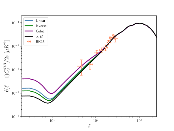
Figure 1: CMB B-mode power spectra for the WI models of Table 1. The data points correspond to the BK18 data (Fig. 3 of [43]).

3 Methods and mock likelihoods

$\Upsilon=C_{C}\frac{T^{3}}{\phi^{2}}$	$c=-2,p=3$	Refs. [47, 48]
$\Upsilon=C_{L}T$	$c=0,p=1$	Ref. [49]
$\Upsilon=C_{I}\frac{\phi^{2}}{T}$	$c=2,p=-1$	Ref. [34]
$\Upsilon=C_{H}H$	$-$	Refs. [50, 51, 52, 32]

Table 1: Summary of the models investigated in this work. We always consider the quartic potential given by eq. 2.6.

CMB forecasting has been widely performed over the years [53, 54, 55, 56, 57, 58, 59, 60, 61, 62, 63, 64, 20, 65, 66, 67, 68, 69, 70, 71, 72, 73, 74], especially with the approval and development of the next generation of CMB dedicated experiments. Surveys scheduled to start operating in this and the next decade aim to achieve precision at cosmological scales not probed before, with the hopes of providing more answers about the cosmos, particularly on the inflationary era. For instance, the LiteBIRD satellite [16, 17] is expected to reach the large scales of the polarization spectra, in particular those of the primordial B-modes, one of last pieces of information needed to futher support the existence of inflation in the early universe. Complementary to these measurements, ground-based surveys are also crucial at smaller scales. The Simons Observatory [21], and the CMB-S4 [19] collaboration, will improve significantly over the Planck results, while also giving us clues to the early-time physics.

3.1 Future CMB surveys

In what follows, we describe the CMB experiments to be considered in our analysis, focusing on parameters necessary to approach the noise modeling. We briefly describe the nature and status of each experiment:

• LiteBIRD: The LiteBIRD satellite project is being lead by the Japan Aerospace Exploration Agency (JAXA) in collaboration with European and North American countries, with operations scheduled to start by the beginning of the 2030s, and focused on measurements of the CMB polarization modes. It will operate in frequencies between 40 GHz and 402 GHz, divided into 15 bands. We work with the 140 GHz band only, as done in [63], but assume a observed sky fraction of $f_{\textrm{sky}}=0.9$.

• CMB-S4: The collaboration consists of large and small aperture telescopes (LAT and SAT, respectively), projected to be located at both South Pole in Antarctica and the Atacama Desert, in Chile. Being a ground-based experiment, its sky fraction coverage is limited, therefore we assume $f_{\textrm{sky}}=0.4$ ($f_{\textrm{sky}}=0.03$) for LAT (SATs). The experiment is set to cover the frequency range of 30$-$270 GHz.

• Simons Observatory: Located in Cerro Toco, also in Chile, the Simons Observatory consists of three SATs and one LAT covering frequencies from 27 to 280 GHz, in six bands. We assume in our analysis, the 93 GHz band , with configurations described in [21], and a sky fraction of $f_{\textrm{sky}}=0.4$ ($f_{\textrm{sky}}=0.1$), for the LAT (SATs).

It is possible to estimate the constraining power of each experiment by assuming different configurations referent to each instrument, such as the sky coverage, temperature and polarization noise, and the scale limit, given by the multipole $\ell$. We use the framework implemented in the MontePython code [75, 76], which builds the mock likelihood given the experimental configuration. Starting from a fiducial model, which is computed with the Cosmic Linear Anisotropy Solving System (CLASS) [77], one can either perform a Fisher matrix forecast, or a MCMC analysis around this model, the latter being the case done here. Given the results obtained in [43], we choose as a starting model a WI implementation with $\log_{10}Q_{\star}=-2$, while setting the remaining cosmological parameters with values consistent with Planck [78], being $\{\omega_{b}=0.02237,\omega_{cdm}=0.12,100\theta_{s}=1.04,\ln(10^{10}A_{s})=3.045\}$. The optical depth at reionization $\tau_{reio}$, is taken as a Gaussian prior of $\tau=0.0544\pm 0.001$, its uncertainty compatible with the one assumed in [63]. Table 2 shows the multipole range for each experiment. We perform our uncertainty analysis and plotting of the confidence contours with GetDist [79].

Survey	T	E	B
SO (LAT)	$30<\ell<8000$	$30<\ell<8000$	$30<\ell<1000$
SO (SAT)	$-$	$30<\ell<8000$	$30<\ell<300$
CMB-S4 (LAT)	$30<\ell<3000$	$30<\ell<5000$	$-$
CMB-S4 (SAT)	$-$	$21<\ell<335$	$21<\ell<335$
LiteBIRD	$-$	$2<\ell<200$	$2<\ell<200$

Table 2: Multipole $\ell$ range for the experiments considered in this work.

3.2 Noise modeling and delensing

In the MontePython implementation, the mock CMB likelihood depends on the $\textbf{C}_{\ell}$ matrix, represented as

$$\textbf{C}_{\ell}=\begin{pmatrix}C_{\ell}^{TT}+N_{\ell}^{TT}&C_{\ell}^{TE}&0\\ C_{\ell}^{TE}&C_{\ell}^{EE}+N_{\ell}^{EE}&0\\ 0&0&C_{\ell}^{BB}+N_{\ell}^{BB}\\ \end{pmatrix}\;.$$ (3.1)

The noise is included as contributions to the diagonal, modeled as [80, 57]

$$N_{\ell}^{XX}=\sigma_{X}^{2}\exp\left({\frac{\ell(\ell+1)\theta_{\textrm{\tiny{FWHM}}}^{2}}{8\ln 2}}\right)\;,$$ (3.2)

where $X$ stands for either temperature $T$ or polarization modes $E,B$, representing the sensitivity in units of $\mu$K-arcmin, while $\theta_{\textrm{\tiny{FWHM}}}$ is the beam width, in units of arcmin. We assume that polarization and temperature noises are related by the multiplicative factor of $\sqrt{2}$, such that $\sigma_{E,B}=\sqrt{2}\sigma_{T}$.

We follow the same approach as [21], in which the instrumental noise has a contribution from low frequency contamination at large scales [81, 82]. This $1/f$ additional noise contributes to the instrumental one as

$$N_{1/f}=1+\left(\frac{\ell}{\ell_{\textrm{knee}}}\right)^{\alpha_{\textrm{knee}}}.$$ (3.3)

The parameters $\ell_{\textrm{knee}}$ and $\alpha_{\textrm{knee}}$ for all experiments considered are the ones displayed in Table 3 of [69]. For LiteBIRD, the beam width and sensitivities are chosen as being correspondent to the 140 GHz band, with values shown in [17, 83]. As for SO, we consider the 93 GHz band of the baseline setting, with parameters displayed in [21]. Finally, for CMB-S4, we follow [63], and choose $\theta_{\textrm{\tiny{FWHM}}}=3$ arcmin and $\sigma_{T}=1\mu$K-arcmin. The chosen approach involving eqs. 3.2 and 3.3 provides a good approximation to the noise curves shown in Fig. 2 of [21]. We also consider the same multipole range of the experiments as done in [69], which are summarized in Table 2. Note that we consider only polarization measurements from LiteBIRD, and avoid the overlap of the $\ell$ for the CMB-S4+LiteBIRD combination. Furthermore, extra care must be taken when we consider B modes in the analysis. As mentioned, the BB power spectrum is dominated by lensed E modes that mask the contribution from primordial perturbations. A technique known as delensing consists of reconstructing the spectrum with reduced lensing power, which depends on the specifics of the instrument and allows us to obtain more information on potential primordial sources at smaller scales. Within the forecasting formalism, one manner of modeling the delensing process is to add an extra source of noise in the $C_{\ell}$ coefficients, such that $C_{\ell}\rightarrow C_{\ell}+N_{\textrm{del}}$, where $N_{\textrm{del}}$ is the noise associated to the delensing process. An approach to this is to simply estimate the delensing level by a parameter $A_{\textrm{lens}}$, such that the $C_{\ell}$s are written as [69]

$$C_{\ell}^{BB}=A_{\textrm{lens}}\left(C_{\ell}^{\textrm{BB},\textrm{lensed}}-C_{\ell}^{\textrm{BB},\textrm{unlensed}}\right)+C_{\ell}^{\textrm{BB},\textrm{unlensed}}.$$ (3.4)

Note that if $A_{\textrm{lens}}=1$, there is no delensing, while $A_{\textrm{lens}}=0$ corresponds to a perfect delensing. For SO, we use $A_{\textrm{lens}}=0.5$, while $A_{\textrm{lens}}=0.27$ is considered for CMB-S4. As for LiteBIRD, we choose a conservative approach and take $A_{\textrm{lens}}=1$ for the experiment.

	Cubic coefficient	Linear coefficient	Inverse coefficient	$\propto H$ coefficient
SO
$\sigma(\Omega_{b}h^{2})$	$0.0000577$	$0.0000553$	$0.0000567$	$0.0000592$
$\sigma(\Omega_{c}h^{2})$	$0.000431$	$0.000437$	$0.000445$	$0.000434$
$\sigma(100\theta)$	$0.000116$	$0.000116$	$0.0000115$	$0.000117$
$\sigma(\tau)$	$0.001$	$0.001$	$0.001$	$0.001$
$\sigma(\ln(10^{10}A_{s}))$	$0.00217$	$0.00212$	$0.00207$	$0.0022$
$\sigma(\log_{10}Q_{\star})$	$0.172$	$0.253$	$0.236$	$0.174$
FoM$/10^{5}$	$15.759$	$14.573$	$14.693$	$15.411$
CMB-S4
$\sigma(\Omega_{b}h^{2})$	$0.0000307$	$0.0000298$	$0.0000295$	$0.0000295$
$\sigma(\Omega_{c}h^{2})$	$0.000365$	$0.000366$	$0.000363$	$0.00362$
$\sigma(100\theta)$	$0.0000809$	$0.0000792$	$0.0000786$	$0.00008$
$\sigma(\tau)$	$0.001$	$0.001$	$0.001$	$0.001$
$\sigma(\ln(10^{10}A_{s}))$	$0.00204$	$0.00198$	$0.002$	$0.00198$
$\sigma(\log_{10}Q_{\star})$	$0.167$	$0.223$	$0.202$	$0.206$
FoM$/10^{5}$	$23.347$	$23.246$	$24.312$	$23.59$
LiteBIRD+CMB-S4
$\sigma(\Omega_{b}h^{2})$	$0.0000311$	$0.0000294$	$0.0000294$	$0.0000297$
$\sigma(\Omega_{c}h^{2})$	$0.000362$	$0.00036$	$0.00035$	$0.000358$
$\sigma(100\theta)$	$0.0000807$	$0.0000805$	$0.000077$	$0.000081$
$\sigma(\tau)$	$0.0009$	$0.000893$	$0.000884$	$0.000891$
$\sigma(\ln(10^{10}A_{s}))$	$0.00183$	$0.00182$	$0.00182$	$0.00181$
$\sigma(\log_{10}Q_{\star})$	$0.1$	$0.15$	$0.138$	$0.139$
FoM$/10^{5}$	$30.223$	$27.556$	$28.508$	$27.59$

Table 3: From left to right, the columns show the projected uncertainties and Figure of Merit values for the cubic, linear, inverse and $\propto H$ dissipation coefficients, according to each experiment.

4 Results

In this section, we present our results, with the general consequences for the warm inflationary picture and its comparison with the standard $\Lambda$CDM$+r$ model results.

4.1 Results for WI models

We now discuss our results for the models chosen. Figures 2,3,4 and 5 show the contours at 68% and 95% CL for the cubic, linear, inverse and $\Upsilon\propto H$ coefficients, respectively. As discussed, we probe the same cosmological parameters as done in [43] to facilitate the comparison between the estimates. We start by comparing projections from the Simons Observatory and CMB-S4, the two ground-based experiments. Fig. 2 shows the result for the cubic model, where we see a significant improvement in the uncertainties for all parameters. This is explicit if we remember the present estimated value of $\log_{10}Q_{\star}=-2.32^{+0.50}_{-0.33}$ [43]. On the other hand, we note that CMB-S4 performs better, especially in estimating the matter fraction, while other parameters remain somewhat similar. It is noticeable here, and this is one of our main results, how the dissipation ratio $Q_{\star}$ is well determined for either SO or CMB-S4, but in particular for the combination of ground and space-borne experiments, represented by the CMB-S4+LiteBIRD analysis. We symmetrize the uncertainties and show their values in Table 3. We find $\sigma(\log_{10}Q_{\star})=0.097$, which is about four times smaller than what was given by the Planck+BK18 analysis performed in [43]. Thus we expect a significant constraining power of future data for these models.

The results for the other models give us the same general conclusions, in which the uncertainties for each experiment are roughly the same, with the notable exception of $\log_{10}Q_{\star}$. In the previous CMB analysis, we have seen that while the cubic model has the best constraints on $\log_{10}Q_{\star}$ (but it is the worst when considering statistical criteria), the other models usually have a larger uncertainty, mainly due to the freedom in the behavior of the primordial power spectrum which is reflected in the curves for the spectral index $n_{s}$ and tensor-to-scalar ratio $r$. Therefore, it is important to know the extent of constraining power of future CMB surveys in order to determine these parameters, since, depending on the model considered, $Q_{\star}$ could span a few orders of magnitude, while still providing a viable inflationary picture.

Table 3 shows that the constraints on $\log_{10}Q_{\star}$ for the linear model have improved by $4.0/4.5$ times when considering SO/CMB-S4, while we have $6.7$ times when the CMB-S4+LiteBIRD combination is considered. Even better restrictions are obtained for the inverse model, which has similar uncertainties as the linear model within current CMB data. Moreover, the model where $\Upsilon\propto H$ has some interesting features. First of all, this is the model that allows the widest range in $Q_{\star}$, where a scenario with a very strong dissipative regime is possible. However, the constraints with SO/CMB-S4 already allow the best constraints of $\log_{10}Q_{\star}$ when compared with the other models, being the same as for the cubic model, while the CMB-S4+LiteBIRD analysis show that the uncertainty in $\log_{10}Q_{\star}$ is also decreased to the same level of the other scenarios considered.

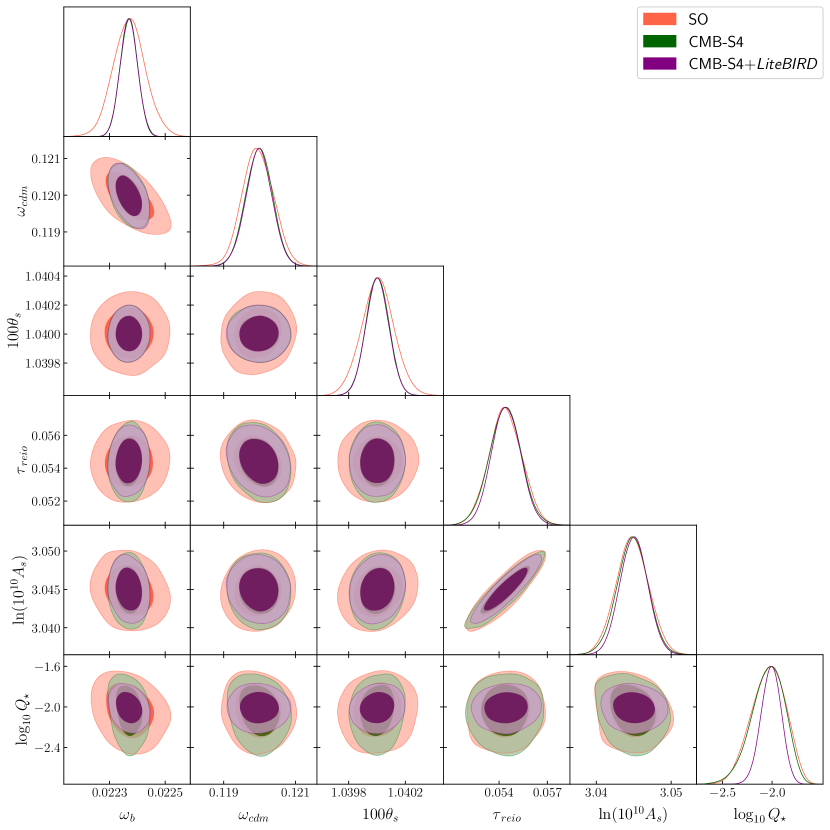
Figure 2: Mock confidence contour plots at 68% and 95% CL (confidence level) and normalized posteriors for the cubic model. We consider the Simons Observatory (red contours), CMB-S4 (green contours) and CMB-S4+LiteBIRD (purple contours).

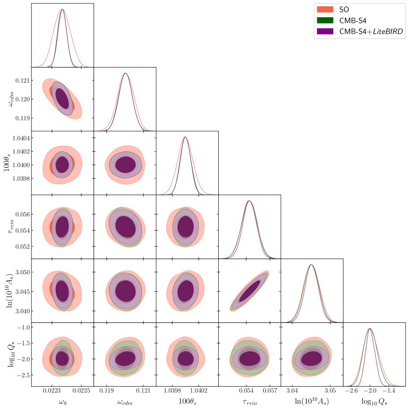
Figure 3: Same as fig. 2, for the linear model.

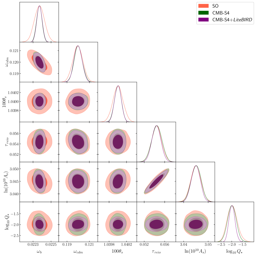
Figure 4: Same as fig. 2, for the inverse model.

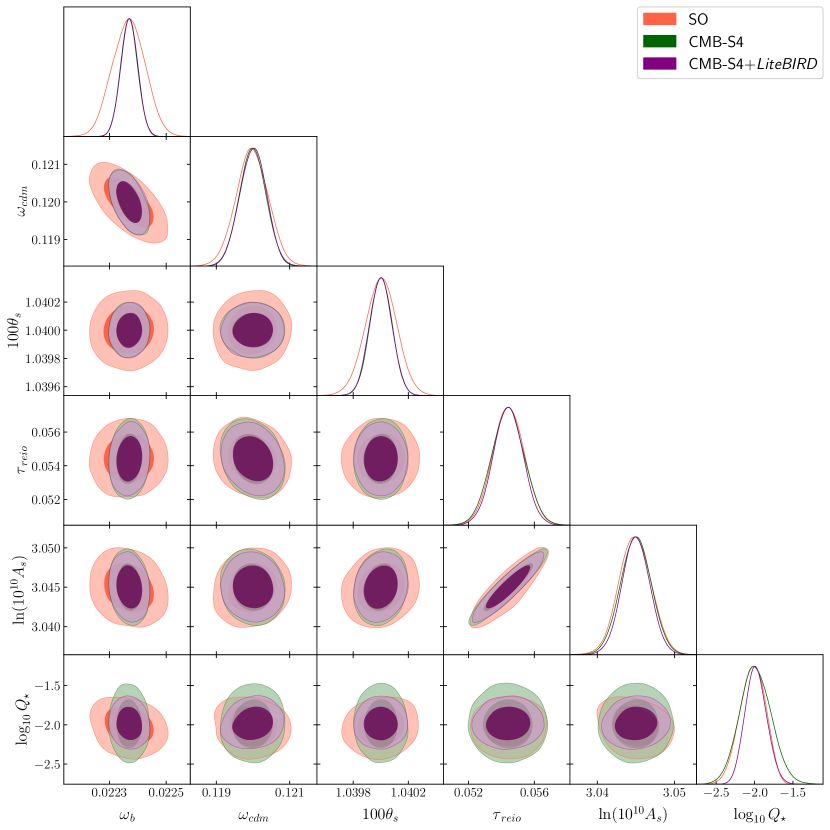
Figure 5: Same as fig. 2, for the $\Upsilon\propto H$ model.

We gather the results on the individual improvement in the uncertainties with respect to the current CMB estimates. Figure 6 shows the ratio $\sigma_{\textrm{current}}/\sigma_{\textrm{s4}}$ for each probed model and experiment, for the six parameters chosen. $\sigma_{\textrm{current}}$ is the symmetrized uncertainty obtained from [43], while $\sigma_{\textrm{s4}}$ corresponds to the values shown in Table 3. For all models, Simons Observatory gives an average of two times better constraints on $\omega_{b},\omega_{c}$ and $100\theta_{s}$, while we note the significant improvement in the dissipation ratio $Q$, represented as $\log_{10}Q_{\star}$. The cubic model is already the best restricted one, but has an improvement of 2.4 times with respect to Planck+BK18 constraints. On the other hand, the $\Upsilon\propto H$ model has a dramatic change, as we estimate an improvement factor of 8.0 in the uncertainty of the parameter.

A somewhat similar behavior happens when we consider CMB-S4 for all models. $\omega_{c}$ and $100\theta_{s}$ constraints are improved by the same order as SO, as well as $\log_{10}Q_{\star}$, which is slightly better for CMB-S4. The main changes are in the baryon fraction $\omega_{c}$, whose uncertainties are more than half of those for SO. Now, for CMB-S4+LiteBIRD, we note that the uncertainties are improved progressively for the cubic, linear, inverse and $\Upsilon\propto H$ models, respectively. In particular, constraints for $\log_{10}Q_{\star}$ in the $\Upsilon\propto H$ model are expected to be $10.1$ times better than the current CMB estimate.

Another way of indicating the experiment’s precision is the measurement of the Figure of Merit (FoM) for each model, which provides the inverse of the area of the ellipse that encloses the 95% confidence limit. Therefore, a higher FoM value indicates greater accuracy of the experiment for that set of parameters. We can define the FoM for $N$ parameters as [84]

$$\text{FoM}=\left(\det F_{ij}^{-1}\right)^{-1/N},$$ (4.1)

where $F_{ij}^{-1}$ is the covariance matrix. As discussed, the most constrained results arise from the CMB-S4+LiteBIRD combination. The CMB-S4 and the Simons Observatory give us very close constraints, depending on the dissipation coefficient considered. Table 3 shows the FoM measurements for the different experiments and models. One can notice that for the Simons observatory, the better accuracy is obtained when considering the cubic dissipation coefficient, with FoM$/10^{5}=15.759$ while CMB-S4 gives FoM$/10^{5}=24.312$ for the inverse model as the highest value. When we look at the the CMB-S4+LiteBIRD combination, we notice the cubic coefficient as the one that provides the best constraints. For this case, we have FoM$/10^{5}=30.223$.

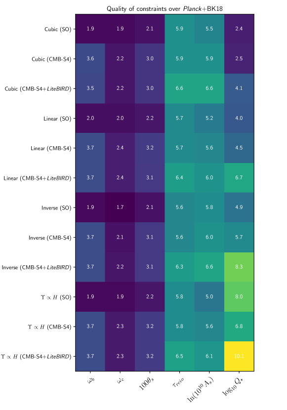
Figure 6: The projected quality on the constraining power of future surveys to the WI models, when compared to current CMB data results, presented in [43]. In the boxes, we show the ratio $\sigma_{\textrm{current}}/\sigma_{\textrm{s4}}$.

4.2 Comparing WI models within a $r=0$ compatibility

For completeness, we also present the prospects for warm inflation in light of the standard $\Lambda$CDM$+r$ model. Current observations are compatible with $r=0$, and it is possible that these results could be maintained, with the upper limit being decreased. We perform a forecast for this model, assuming a $r=0$ detection, with results shown in Fig. 6, for the same mock likelihoods discussed previously. In the figure, we show the predicted $n_{s}-r$ contours for each experiment, compared with the predictions for each WI model.

Regardless of the choice of survey, the cubic WI model (gray curve) becomes excluded by the improved constraints on $r$; this not only shows how warm inflationary models can be now distinguished even better, but also tells us how in the event of a non-detection of a primordial gravitational wave signal, possibly dozens of other inflationary models will also be excluded by data. On the other hand, such scenario is somewhat more favorable to WI models, which allow in general a decreasing tensor-to-scalar ratio with respect to cold inflationary models. The other WI models presented are still in good agreement with a lower $r$, as also seen in the figure. For instance, the linear model, shown by the blue curve in the plot, is not only favored statistically with respect to the Starobinsky model [43], but is also the one that better agrees with the $1\sigma$ contour of the CMB-S4+LiteBIRD projection. Also, viable WI models in the very strong regime ($Q\gg 1$) start to become stronger candidates as well, since they generally predict extremely low values of $r$.

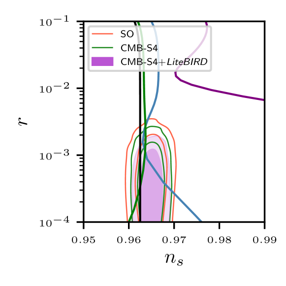
Figure 7: Projected constraints on the scalar spectral index $n_{s}$ and tensor-to-scalar ratio $r$ for the $\Lambda$CDM$+r$ model, for SO (red contour), CMB-S4 (green contour) and CMB-S4+LiteBIRD (filled violet contours). Also in the plot are the predictions for the different WI models investigated in this work, being the cubic (purple curve), linear (blue curve), inverse (green curve), and the $\propto H$ model, represented by the black curve.

5 Discussion and Conclusions

The next decade CMB data is highly anticipated, not only because it will open a new era in precision cosmology, after the successful findings of WMAP and Planck, but also for the prospects of further exploring the parameter space of a variety of early-time physical models, including inflation. As there are plenty of viable models currently, it becomes urgent to start properly distinguishing these scenarios, as well as looking for specific phenomena directly related to a possible inflationary period. The most searched signal from primordial times is arguably the production of gravitational waves during inflation, which manifest themselves through a polarization pattern in the CMB. If existent, these B modes are actually extremely difficult to detect, due to the weakness of the signal, and the astrophysical contaminants that should be properly extracted in the data processing. Thus, it is important to assess the readiness of developing experiments in performing these measurements, while also dealing with different kinds of noise that will permeate the observations.

In this work, we performed a forecast to investigate the sensitivity with which future CMB experiments will constrain early-time physics within the warm inflation scenario, which has been shown to be promising due to a solid theoretical background, rich phenomenology, and the possibility of uniting the eras of inflation and reheating in the same framework. Specifically, we explore a model given by a quartic potential, considering four different forms of the dissipation coefficient. We then have forecast restrictions on these models using configurations of Simons Observatory, CMB-S4, and a combination of CMB-S4 and LiteBIRD.

A summary of the main findings of this work are displayed in Table 3, which shows the projected uncertainties in the cosmological parameters, and Figure 6, in which the improvement over current CMB constraints are shown. The improvement in the uncertainties is compatible with the findings in [63], for instance, where a stage IV CMB forecast was also performed, but for an extended $\Lambda$CDM model with neutrinos. We see how especially the combination of CMB-S4 and LiteBIRD could lead to at least $\sim$2 times smaller uncertainties with respect to current data. As seen in Figure 6, the consequences are even more explicit for the logarithm of the dissipation ratio $\log_{10}Q_{\star}$, which has its uncertainties reduced by at least 4.1 times. Another important discussion is the possibility of a non-detection of a primordial gravitational signal, leading to results compatible with $r=0$, which is the case currently. We perform an analysis for the $\Lambda$CDM$+r$ model, and compare the $n_{s}-r$ contours with the predictions for each WI model. Since we have around $r<3\times 10^{-3}$ at 95% CL, the cubic WI model becomes excluded; this tells us that future CMB data should allow us to distinguish different dissipation coefficients already at the $n_{s}-r$ level. Moreover, the linear model with a quartic potential, compatible with the proposal in [49], becomes a even more viable option in the WI construction. Finally, as mentioned, a $r=0$ result can be favorable to WI models in the strong dissipation regime, in which the tensor-to-scalar ratio is typically low, and few well motivated cold inflationary models are actually compatible with such projections.

References

- Hinshaw et al. [2013] G. Hinshaw et al. (WMAP), Astrophys. J. Suppl. 208, 19 (2013), arXiv:1212.5226 [astro-ph.CO] .
- Aghanim et al. [2020a] N. Aghanim et al. (Planck), Astron. Astrophys. 641, A1 (2020a), arXiv:1807.06205 [astro-ph.CO] .
- Aghanim et al. [2020b] N. Aghanim et al. (Planck), Astron. Astrophys. 641, A6 (2020b), [Erratum: Astron.Astrophys. 652, C4 (2021)], arXiv:1807.06209 [astro-ph.CO] .
- Ade et al. [2021] P. A. R. Ade et al. (BICEP, Keck), Phys. Rev. Lett. 127, 151301 (2021), arXiv:2110.00483 [astro-ph.CO] .
- Guth [1981] A. H. Guth, Phys. Rev. D 23, 347 (1981).
- Starobinsky [1980] A. A. Starobinsky, Phys. Lett. B 91, 99 (1980).
- Linde [1982] A. D. Linde, Phys. Lett. B 108, 389 (1982).
- Albrecht et al. [1982] A. Albrecht, P. J. Steinhardt, M. S. Turner, and F. Wilczek, Phys. Rev. Lett. 48, 1437 (1982).
- Abbott et al. [1982] L. F. Abbott, E. Farhi, and M. B. Wise, Phys. Lett. B 117, 29 (1982).
- Kofman et al. [1994] L. Kofman, A. D. Linde, and A. A. Starobinsky, Phys. Rev. Lett. 73, 3195 (1994), arXiv:hep-th/9405187 .
- Kofman et al. [1997] L. Kofman, A. D. Linde, and A. A. Starobinsky, Phys. Rev. D 56, 3258 (1997), arXiv:hep-ph/9704452 .
- Ade et al. [2016] P. A. R. Ade et al. (BICEP2, Keck Array), Phys. Rev. Lett. 116, 031302 (2016), arXiv:1510.09217 [astro-ph.CO] .
- Ade et al. [2018] P. A. R. Ade et al. (BICEP2, Keck Array), Phys. Rev. Lett. 121, 221301 (2018), arXiv:1810.05216 [astro-ph.CO] .
- Tristram et al. [2021] M. Tristram et al., Astron. Astrophys. 647, A128 (2021), arXiv:2010.01139 [astro-ph.CO] .
- Tristram et al. [2022] M. Tristram et al., Phys. Rev. D 105, 083524 (2022), arXiv:2112.07961 [astro-ph.CO] .
- Matsumura et al. [2014] T. Matsumura et al., J. Low Temp. Phys. 176, 733 (2014), arXiv:1311.2847 [astro-ph.IM] .
- Hazumi et al. [2019] M. Hazumi et al., J. Low Temp. Phys. 194, 443 (2019).
- Allys et al. [2023] E. Allys et al. (LiteBIRD), PTEP 2023, 042F01 (2023), arXiv:2202.02773 [astro-ph.IM] .
- Abazajian et al. [2016] K. N. Abazajian et al. (CMB-S4), (2016), arXiv:1610.02743 [astro-ph.CO] .
- Abazajian et al. [2022] K. Abazajian et al. (CMB-S4), Astrophys. J. 926, 54 (2022), arXiv:2008.12619 [astro-ph.CO] .
- Ade et al. [2019] P. Ade et al. (Simons Observatory), JCAP 02, 056 (2019), arXiv:1808.07445 [astro-ph.CO] .
- Berera [1995] A. Berera, Phys. Rev. Lett. 75, 3218 (1995), arXiv:astro-ph/9509049 .
- Maia and Lima [1999] J. M. F. Maia and J. A. S. Lima, Phys. Rev. D 60, 101301 (1999), arXiv:astro-ph/9910568 .
- Hall et al. [2004] L. M. H. Hall, I. G. Moss, and A. Berera, Phys. Rev. D 69, 083525 (2004), arXiv:astro-ph/0305015 .
- Berera [2023] A. Berera, Universe 9, 272 (2023), arXiv:2305.10879 [hep-ph] .
- Kamali et al. [2023] V. Kamali, M. Motaharfar, and R. O. Ramos, Universe 9, 124 (2023), arXiv:2302.02827 [hep-ph] .
- Berera et al. [2009] A. Berera, I. G. Moss, and R. O. Ramos, Rept. Prog. Phys. 72, 026901 (2009), arXiv:0808.1855 [hep-ph] .
- Bastero-Gil et al. [2011a] M. Bastero-Gil, A. Berera, and R. O. Ramos, JCAP 09, 033 (2011a), arXiv:1008.1929 [hep-ph] .
- Benetti and Ramos [2017] M. Benetti and R. O. Ramos, Phys. Rev. D 95, 023517 (2017), arXiv:1610.08758 [astro-ph.CO] .
- Bastero-Gil et al. [2018] M. Bastero-Gil, S. Bhattacharya, K. Dutta, and M. R. Gangopadhyay, JCAP 02, 054 (2018), arXiv:1710.10008 [astro-ph.CO] .
- Arya et al. [2018] R. Arya, A. Dasgupta, G. Goswami, J. Prasad, and R. Rangarajan, JCAP 02, 043 (2018), arXiv:1710.11109 [astro-ph.CO] .
- Motaharfar et al. [2019] M. Motaharfar, V. Kamali, and R. O. Ramos, Phys. Rev. D 99, 063513 (2019), arXiv:1810.02816 [astro-ph.CO] .
- Arya and Rangarajan [2020] R. Arya and R. Rangarajan, Int. J. Mod. Phys. D 29, 2050055 (2020), arXiv:1812.03107 [astro-ph.CO] .
- Bastero-Gil et al. [2021] M. Bastero-Gil, A. Berera, R. O. Ramos, and J. a. G. Rosa, Phys. Lett. B 813, 136055 (2021), arXiv:1907.13410 [hep-ph] .
- Das et al. [2020] S. Das, G. Goswami, and C. Krishnan, Phys. Rev. D 101, 103529 (2020), arXiv:1911.00323 [hep-th] .
- Kamali et al. [2020] V. Kamali, M. Motaharfar, and R. O. Ramos, Phys. Rev. D 101, 023535 (2020), arXiv:1910.06796 [gr-qc] .
- Benetti et al. [2019] M. Benetti, L. Graef, and R. O. Ramos, JCAP 10, 066 (2019), arXiv:1907.03633 [astro-ph.CO] .
- Berera and Calderón [2019] A. Berera and J. R. Calderón, Phys. Rev. D 100, 123530 (2019), arXiv:1910.10516 [hep-ph] .
- Das and Ramos [2020] S. Das and R. O. Ramos, Phys. Rev. D 102, 103522 (2020), arXiv:2007.15268 [hep-th] .
- Santos et al. [2023] F. B. M. d. Santos, R. Silva, S. S. da Costa, M. Benetti, and J. S. Alcaniz, Eur. Phys. J. C 83, 178 (2023), arXiv:2209.06153 [astro-ph.CO] .
- Arya and Mishra [2022] R. Arya and A. K. Mishra, Phys. Dark Univ. 37, 101116 (2022), arXiv:2204.02896 [astro-ph.CO] .
- Arya et al. [2024] R. Arya, R. K. Jain, and A. K. Mishra, JCAP 02, 034 (2024), arXiv:2302.08940 [astro-ph.CO] .
- Santos et al. [2024] F. B. M. d. Santos, R. de Souza, and J. S. Alcaniz, JCAP 10, 071 (2024), arXiv:2407.18891 [astro-ph.CO] .
- Graham and Moss [2009] C. Graham and I. G. Moss, JCAP 07, 013 (2009), arXiv:0905.3500 [astro-ph.CO] .
- Bastero-Gil and Berera [2009] M. Bastero-Gil and A. Berera, Int. J. Mod. Phys. A 24, 2207 (2009), arXiv:0902.0521 [hep-ph] .
- Bastero-Gil et al. [2011b] M. Bastero-Gil, A. Berera, and R. O. Ramos, JCAP 07, 030 (2011b), arXiv:1106.0701 [astro-ph.CO] .
- Bastero-Gil et al. [2013] M. Bastero-Gil, A. Berera, R. O. Ramos, and J. G. Rosa, JCAP 01, 016 (2013), arXiv:1207.0445 [hep-ph] .
- Berghaus et al. [2020] K. V. Berghaus, P. W. Graham, and D. E. Kaplan, JCAP 03, 034 (2020), [Erratum: JCAP 10, E02 (2023)], arXiv:1910.07525 [hep-ph] .
- Bastero-Gil et al. [2016] M. Bastero-Gil, A. Berera, R. O. Ramos, and J. G. Rosa, Phys. Rev. Lett. 117, 151301 (2016), arXiv:1604.08838 [hep-ph] .
- Bolotin et al. [2014] Y. L. Bolotin, A. Kostenko, O. A. Lemets, and D. A. Yerokhin, Int. J. Mod. Phys. D 24, 1530007 (2014), arXiv:1310.0085 [astro-ph.CO] .
- von Marttens et al. [2020] R. von Marttens, H. A. Borges, S. Carneiro, J. S. Alcaniz, and W. Zimdahl, Eur. Phys. J. C 80, 1110 (2020), arXiv:1909.10336 [gr-qc] .
- Barbosa et al. [2017] C. M. S. Barbosa, H. Velten, J. C. Fabris, and R. O. Ramos, Phys. Rev. D 96, 023527 (2017), arXiv:1702.07040 [astro-ph.CO] .
- Okamoto and Hu [2003] T. Okamoto and W. Hu, Phys. Rev. D 67, 083002 (2003), arXiv:astro-ph/0301031 .
- Lesgourgues et al. [2006] J. Lesgourgues, L. Perotto, S. Pastor, and M. Piat, Phys. Rev. D 73, 045021 (2006), arXiv:astro-ph/0511735 .
- Perotto et al. [2006] L. Perotto, J. Lesgourgues, S. Hannestad, H. Tu, and Y. Y. Y. Wong, JCAP 10, 013 (2006), arXiv:astro-ph/0606227 .
- Smith et al. [2012] K. M. Smith, D. Hanson, M. LoVerde, C. M. Hirata, and O. Zahn, JCAP 06, 014 (2012), arXiv:1010.0048 [astro-ph.CO] .
- Wu et al. [2014] W. L. K. Wu, J. Errard, C. Dvorkin, C. L. Kuo, A. T. Lee, P. McDonald, A. Slosar, and O. Zahn, Astrophys. J. 788, 138 (2014), arXiv:1402.4108 [astro-ph.CO] .
- Errard et al. [2016] J. Errard, S. M. Feeney, H. V. Peiris, and A. H. Jaffe, JCAP 03, 052 (2016), arXiv:1509.06770 [astro-ph.CO] .
- Namikawa and Nagata [2015] T. Namikawa and R. Nagata, JCAP 10, 004 (2015), arXiv:1506.09209 [astro-ph.CO] .
- Finelli et al. [2018] F. Finelli et al. (CORE), JCAP 04, 016 (2018), arXiv:1612.08270 [astro-ph.CO] .
- Green et al. [2017] D. Green, J. Meyers, and A. van Engelen, JCAP 12, 005 (2017), arXiv:1609.08143 [astro-ph.CO] .
- Manzotti et al. [2017] A. Manzotti et al. (SPT, Herschel), Astrophys. J. 846, 45 (2017), arXiv:1701.04396 [astro-ph.CO] .
- Brinckmann et al. [2019] T. Brinckmann, D. C. Hooper, M. Archidiacono, J. Lesgourgues, and T. Sprenger, JCAP 01, 059 (2019), arXiv:1808.05955 [astro-ph.CO] .
- Baleato Lizancos et al. [2021] A. Baleato Lizancos, A. Challinor, and J. Carron, Phys. Rev. D 103, 023518 (2021), arXiv:2010.14286 [astro-ph.CO] .
- Hotinli et al. [2022] S. C. Hotinli, J. Meyers, C. Trendafilova, D. Green, and A. van Engelen, JCAP 04, 020 (2022), arXiv:2111.15036 [astro-ph.CO] .
- Baleato Lizancos and Ferraro [2022] A. Baleato Lizancos and S. Ferraro, Phys. Rev. D 106, 063534 (2022), arXiv:2205.09000 [astro-ph.CO] .
- Hamann and Malhotra [2022] J. Hamann and A. Malhotra, JCAP 12, 015 (2022), arXiv:2209.00827 [astro-ph.CO] .
- Modak et al. [2023] T. Modak, L. Röver, B. M. Schäfer, B. Schosser, and T. Plehn, SciPost Phys. 15, 047 (2023), arXiv:2210.05698 [astro-ph.CO] .
- Bahr-Kalus et al. [2023] B. Bahr-Kalus, D. Parkinson, and R. Easther, Mon. Not. Roy. Astron. Soc. 520, 2405 (2023), arXiv:2212.04115 [astro-ph.CO] .
- Belkner et al. [2024] S. Belkner, J. Carron, L. Legrand, C. Umiltà, C. Pryke, and C. Bischoff (CMB-S4), Astrophys. J. 964, 148 (2024), arXiv:2310.06729 [astro-ph.CO] .
- Fuskeland et al. [2023] U. Fuskeland et al. (LiteBIRD), Astron. Astrophys. 676, A42 (2023), arXiv:2302.05228 [astro-ph.CO] .
- Namikawa et al. [2024] T. Namikawa et al. (LiteBIRD), JCAP 06, 010 (2024), arXiv:2312.05194 [astro-ph.CO] .
- Lonappan et al. [2024] A. I. Lonappan et al. (LiteBIRD), JCAP 06, 009 (2024), arXiv:2312.05184 [astro-ph.CO] .
- Chen et al. [2024] W.-Z. Chen, Y. Liu, S. Li, B. Hu, and H. Li, (2024), arXiv:2403.16726 [astro-ph.CO] .
- Brinckmann and Lesgourgues [2019] T. Brinckmann and J. Lesgourgues, Phys. Dark Univ. 24, 100260 (2019), arXiv:1804.07261 [astro-ph.CO] .
- Audren et al. [2013] B. Audren, J. Lesgourgues, K. Benabed, and S. Prunet, JCAP 1302, 001 (2013), arXiv:1210.7183 [astro-ph.CO] .
- Blas et al. [2011] D. Blas, J. Lesgourgues, and T. Tram, JCAP 07, 034 (2011), arXiv:1104.2933 [astro-ph.CO] .
- Akrami et al. [2020] Y. Akrami et al. (Planck), Astron. Astrophys. 641, A10 (2020), arXiv:1807.06211 [astro-ph.CO] .
- Lewis [2019] A. Lewis, (2019), arXiv:1910.13970 [astro-ph.IM] .
- Ng and Liu [1999] K.-W. Ng and G.-C. Liu, Int. J. Mod. Phys. D 8, 61 (1999), arXiv:astro-ph/9710012 .
- Maino et al. [2002] D. Maino, C. Burigana, K. M. Gorski, N. Mandolesi, and M. Bersanelli, Astron. Astrophys. 387, 356 (2002), arXiv:astro-ph/0202271 .
- Donzelli et al. [2009] S. Donzelli, F. K. Hansen, M. Liguori, and D. Maino, Astrophys. J. 706, 1226 (2009), arXiv:0907.4650 [astro-ph.CO] .
- Paoletti and Finelli [2019] D. Paoletti and F. Finelli, JCAP 11, 028 (2019), arXiv:1910.07456 [astro-ph.CO] .
- Alonso et al. [2017] D. Alonso, E. Bellini, P. G. Ferreira, and M. Zumalacárregui, Phys. Rev. D 95, 063502 (2017), arXiv:1610.09290 [astro-ph.CO] .