Taming Scalable Visual Tokenizer for Autoregressive Image Generation

Abstract

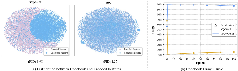
Figure 2: Effects of Distribution Gap on Codebook Usage. (a) T-SNE of the codebook (16,384 codebook size and 256 dimension) and sampled encoder features. (b) Codebook usage curve. The partial-update strategy adopted by VQGAN broadens the distribution gap between encoded features and non-activated codes, while those of IBQ based on all-codes updating are evenly mixed, maintaining a high codebook usage ($\sim$96%) throughout the training. Fully leveraging the codebook significantly improves the reconstruction quality.

Existing vector quantization (VQ) methods struggle with scalability, largely attributed to the instability of the codebook that undergoes partial updates during training. The codebook is prone to collapse as utilization decreases, due to the progressively widening distribution gap between non-activated codes and visual features. To solve the problem, we propose Index Backpropagation Quantization (IBQ), a new VQ method for the joint optimization of all codebook embeddings and the visual encoder. Applying a straight-through estimator on the one-hot categorical distribution between the encoded feature and codebook, all codes are differentiable and maintain a consistent latent space with the visual encoder. IBQ enables scalable training of visual tokenizers and, for the first time, achieves a large-scale codebook ($2^{18}$) with high dimension ($256$) and high utilization. Experiments on the standard ImageNet benchmark demonstrate the scalability and superiority of IBQ, achieving competitive results on both reconstruction ($1.00$ rFID) and autoregressive visual generation ($2.05$ gFID). The code and models are available at https://github.com/TencentARC/SEED-Voken.

Figure 1: Reconstruction and generation samples of IBQ. We show 1024 $\times$ 1024 reconstructed samples (top) and 256 $\times$ 256 generated samples (middle and bottom).

1 Introduction

Given the remarkable scalability and generalizability of autoregressive transformers [29, 2] in large language models [17, 26], recent efforts have been made to extend this success to visual generation [28, 6, 24, 25]. The common practice is to discretize images into tokens using vector quantization (VQ) before applying autoregressive transformers for discrete sequence modeling through next-token prediction.

Existing studies on autoregressive visual generation primarily aim to improve the reconstruction performance of visual tokenizers [6, 31, 32] or to refine the autoregressive modeling of transformers [25, 24, 16, 14]. The improvement of visual tokenizers is crucial, given that it can markedly amplify the potential performance of ensuing autoregressive models. Intuitively, scaling visual tokenizers by increasing the codebook size and embedding dimension could help bridge the gap between discrete and continuous representations, thereby mitigating the information loss associated with discrete tokens. However, it is noteworthy that current visual tokenizers [31, 24] have not demonstrated such scaling properties.

Empirical research [6, 24] has revealed that current VQ methods struggle with scalability due to the inherent tendency of the codebook to collapse. This arises because these methods only optimize limited selected codes during each backpropagation. Such a widely-adopted partial update strategy gradually broadens the distribution gap between non-activated codes and the visual encoder’s representation space, making the non-activated codes further less likely to be selected. As shown in Fig. 2, VQGAN [6] almost fails when scaling both codebook size (i.e., $16,384$) and embedding dimension (i.e., $256$) simultaneously. Only a small amount of codes share the same distribution with the visual encoder, and the codebook usage degrades from $68\%$ to $0.002\%$ after training one epoch.

To tackle the challenge, we introduce a new VQ method, namely, Index Backpropagation Quantization (IBQ). It globally updates the entire codebook in each backward process to ensure consistency with the distribution of the visual encoder. In such a way, all codes have the same probability of being selected, resulting in a high utilization of the codebook throughout the training process. Specifically, rather than directly applying the straight-through estimator [1] to the selected codes, we employ this reparameterization approach on the categorical distribution between visual features and all codebook embeddings, thereby rendering all codes differentiable. As shown in Fig. 2, the sampled visual features and the codebook embeddings from IBQ are evenly mixed. IBQ keeps a high codebook usage ($\sim 96\%$) throughout the training process. Fully leveraging the codebook effectively enhances the representation capacity, as demonstrated by the superior reconstruction of IBQ ($1.37$ rFID) compared to VQGAN ($3.98$ rFID).

Experiments on the standard ImageNet benchmark validate the scalability and superiority of our method in both reconstruction and generation. We conducted an in-depth study on the scaling law of the IBQ tokenizer from three aspects: codebook size, code dimension, and model size. We observed that the reconstruction performance or codebook usage significantly increases when scaling up tokenizer training. To our knowledge, IBQ is the pioneering work to train an extremely large codebook (i.e., $262,144$) with a relatively large code dimension (i.e., $256$). This achievement has resulted in state-of-the-art reconstruction performance, achieving a $1.00$ rFID. We employed the IBQ tokenizer in a vanilla autoregressive transformer for visual generation, training models of varying sizes from 300M to 2.1B, and achieved competitive results.

In summary, our contributions are threefold:

• We propose a simple yet effective vector quantization method, dubbed Index Backpropagation Quantization (IBQ), for training scalable visual tokenizers.

• We study the scaling properties of IBQ by increasing codebook size, code dimension, and model size. IBQ for the first time trains a super large codebook ($2^{18}$) with a large dimension ($256$) and high usage, achieving state-of-the-art reconstruction performance.

• We present a family of vanilla autoregressive image generation models ranging from 300M to 2.1B, remarkably outperforming competing methods, e.g., LlamaGen [24], and Open-MAGVIT2 [16].

2 Related Work

2.1 Vector Quantization

At the core of visual tokenizers is vector quantization, which maps the visual signals into discrete tokens. VQ-VAE [28] proposes an encoder-quantizer-decoder structure and uses a learnable codebook as the discrete representation space. VQ-VAE2 [19] introduces multi-scale hierarchical VQ-VAE to enhance local features. VQGAN [6] further uses adversarial loss and perceptual loss for good perceptual quality. RQ-VAE [13] and DQ-VAE [9] improve VQGAN by residual quantization and dynamic quantization respectively. To improve codebook utilization for large-size codebooks, some works try to decrease code dimension [31, 24]. Following this observation, MAGVIT-v2 [32] reduces the code dimension to zero, and significantly enlarges the codebook size to $2^{18}$ with Lookup-Free Quantization. Instead of joint optimization of the model and codebook, VQGAN-LC [36] extends the codebook size to 100,000 by utilizing a frozen codebook with a trainable projector.

Existing VQ methods suffer from codebook collapse when scaling up tokenzier, and usually use a small codebook size or low code dimension, which limits the representational capacity of the codebook. In contrast, our proposed IBQ shows consistent improvements when scaling up code dimension, codebook size and model size.

2.2 Tokenized Visual Generation

Tokenizers map continuous visual signals into a discrete token sequence. For subsequent visual generation, there are two approaches, including non-autoregressive (NAR) and autoregressive (AR) generation. NAR [3, 32] usually adopts BERT-style transformers to predict masked tokens. For inference, these methods generate all tokens of an image simultaneously, and iteratively refine the generated images conditioned on the previous generation. In contrast, AR models perform next-token prediction in a raster-scan manner. VQGAN [6] adopts GPT2-medium architecture, while LlamaGen [24] employs Llama [26] for scalable image generation. VAR [25] extends “next-token prediction” to “next-scale prediction” and introduces adaptive normalization (AdaLN [18]) to improve visual generation quality. Open-MAGVIT2 [16] introduces asymmetric token factorization for super-large codebook learning. In this paper, we follow vanilla autoregressive visual generation, and adopt Llama [26] with AdaLn [18] for image generation.

Algorithm 1 Pseudocode of IBQ in a PyTorch-like style

⬇

def IBQ(z, codebook):

’’’

␣␣␣␣z:␣visual␣feature␣map␣(B␣*␣h␣*␣w,␣D)

␣␣␣␣␣␣␣␣B:␣batch␣size

␣␣␣␣␣␣␣␣h:␣height␣of␣feature␣map

␣␣␣␣␣␣␣␣w:␣width␣of␣feature␣map

␣␣␣␣␣␣␣␣D:␣feature␣dimension

␣␣␣␣codebook:␣(K,␣D)

␣␣␣␣␣␣␣␣K:␣codebook␣size

␣␣␣␣␣␣␣␣D:␣code␣dimension

␣␣␣␣’’’

logits = mm(z, codebook.T) # (B * h * w, K)

Ind_soft = softmax(logits, dim=1) # (B * h * w, K)

_, indices = soft_one_hot.max(dim=1)

Ind_hard = onehot(indices) # (B * h * w, K)

Ind = Ind_hard - Ind_soft.detach() + Ind_soft

z_q = mm(Ind, codebook) # (B * h * w, D)

return z_q

 mm: matrix multiplication; onehot: transfer index into one-hot vector.

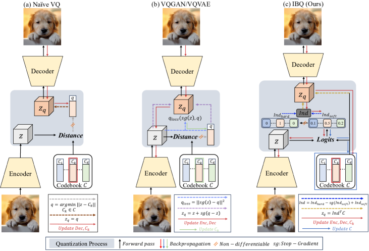
Figure 3: Gradient flow of different VQ methods. Naïve VQ and VQGAN/VQVAE only update the selected codes in each backward process. IBQ updates all codes simultaneously by transferring the gradients of soft one-hot categorical distribution to hard one-hot index.

3 Method

Our framework consists of two stages. The first stage is to learn a scalable visual tokenizer with high codebook utilization via Index Backpropagation Quantization. In the second stage, we use an autoregressive transformer for visual generation by next-token prediction.

3.1 Preliminary

Vector quantization (VQ) maps continuous visual signals into discrete tokens with a fixed-size codebook $\mathcal{C}\in\mathbb{R}^{K\times D}$, where $K$ is the codebook size and $D$ is the code dimension. Given an image $\mathcal{I}\in\mathbb{R}^{H\times W\times 3}$, VQ first utilizes an encoder to project the image into the feature map $\mathcal{Z}\in\mathbb{R}^{h\times w\times D}$, where $h=H/p$, $w=W/p$, and $p$ is the downsample ratio. Then the feature map is quantized into $\mathcal{Q}\in\mathbb{R}^{h\times w\times D}$ as discrete representations with the codebook. Finally, the decoder reconstructs the image given the quantized features.

For quantization, previous methods typically calculate the Euclidean distance between each visual feature $z\in\mathbb{R}^{D}$ and all codes of the codebook, and then select the closest code as its discrete representation [28, 6]. Since the $\operatorname*{arg\,min}$ operation in quantization is non-differentiable, they apply the straight-through estimator on selected codes to copy the gradients from the decoder, to optimize the encoder simultaneously. The quantization process is as follows:

$$q =\operatorname*{arg\,min}_{\mathcal{C}_{k}\in\mathcal{C}}||z-\mathcal{C}_{k}||\in\mathbb{R}^{D},$$ (1)

$$z_{q} =z+\text{sg}[q-z],$$ (2)

where sg$[\cdot]$ is stop-gradient operation.

The partial updating strategy (i.e., only selected codes are optimized) adopted by these methods progressively widens the distribution gap between visual features and non-activated codes. It incurs the instability during training due to the codebook collapse, which hampers the scalability of the visual tokenizer.

3.2 Index Backpropagation Quantization

Quantization. To ensure the consistent distribution between the codebook and encoded features through the training, we introduce an all-codes updating method, Index Backpropagation Quantization (IBQ). At the core of IBQ is passing gradients backward to all codes of the codebook, instead of the selected codes only. Algorithm 1 provides the pseudo-code of IBQ.

Specifically, we first perform dot product between the given visual feature $z$ and all code embeddings as logits and get probabilities (soft one-hot) by softmax function.

logits $$=[z^{T}\mathcal{C}_{1},z^{T}\mathcal{C}_{2},\cdots,z^{T}\mathcal{C}_{K}]^{T}\in\mathbb{R}^{K},$$ (3)

$$\text{Ind}_{\text{soft}} =\text{softmax}(\text{logits}),$$ (4)

$$\text{Ind}_{\text{hard}} =\text{One-Hot}(\text{argmax}(\text{Ind}_{\text{soft}})).$$ (5)

Then we copy the gradients of soft one-hot categorical distribution to hard one-hot index:

$$\text{Ind}=\text{Ind}_{\text{hard}}-\text{sg}[\text{Ind}_{\text{soft}}]+\text{Ind}_{\text{soft}}.$$ (6)

Given the index, the quantized feature is obtained by:

$$z_{q}=\text{Ind}^{T}\mathcal{C}.$$ (7)

In this way, we can pass the gradients to all codes of the codebook via index. By Index Backpropagation Quantization, the distribution of the whole codebook and encoded features remains consistent throughout completed training, thus gaining a high codebook utilization.

Training Losses. Similar to VQGAN [6], the tokenizer is optimized with a combination of losses:

$$\mathcal{L} =\mathcal{L}_{R}+\mathcal{L}_{Q}+\mathcal{L}_{P}+\mathcal{L}_{G}+\mathcal{L}_{E},$$ (8)

where $\mathcal{L}_{R}$ is reconstruction loss of image pixels, $\mathcal{L}_{Q}$ is quantization loss between the selected code embeddings and encoded features, $\mathcal{L}_{P}$ is perceptual loss from LPIPS [34], $\mathcal{L}_{G}$ is adversarial loss with PatchGAN discriminator [10] to enhance the image quality, and $\mathcal{L}_{E}$ is entropy penalty to encourage codebook utilization.

We further introduce double quantization loss, to force the selected code embeddings and given encoded visual features towards each other.

$${z_{q}}^{\prime}= \text{Ind}_{\text{hard}}^{T}\cdot[\mathcal{C}_{1},\mathcal{C}_{2},\cdots,\mathcal{C}_{K}],$$ (9)

$$\begin{split}\mathcal{L}_{Q}=&||z_{q}-z||^{2}+\\ &||\text{sg}[z]-{z_{q}}^{\prime}||^{2}+\beta||z-\text{sg}[{z_{q}}^{\prime}]||^{2}.\end{split}$$ (10)

Discussion with other VQ methods. Vector quantization (VQ) discretizes a continuous visual feature into a quantized code with a fix-size codebook. Naive VQ selects the code with the closest Euclidean distance to the given visual feature. Since the $\operatorname*{arg\,min}$ operation is non-differentiable, the gradient flow back to the encoder is truncated, and only the parameters of the decoder and the selected codes can be updated. Inspired by straight-through gradient estimator [1], VQ-VAE and VQGAN copy the gradients from the decoder to the encoder for gradient approximation. They also adopt quantization loss to optimize the selected codes towards the encoded features. Consequently, the VQ model can be trained in an end-to-end manner. Despite progress has been made, these VQ methods struggle to scale up tokenizers for better representation capacity.

As shown in Fig. 3, existing VQ methods simply optimize a limited number of codes towards encoded features within each backward process. It progressively broadens the distribution gap between the non-activated codes and the encoded features, eventually leading to codebook collapse. And this situation becomes more severe with the code dimension and codebook size increase. Rather than directly applying the straight-through estimator [1] on the selected codes, we employ this parameterization approach on the categorical distribution between visual features and all codebook embeddings to enable gradients backward to all codes. In such a way, the distribution between the whole codebook and the encoded features remains consistent throughout the training process. Consequently, IBQ achieves an extremely large codebook with high code dimension and utilization.

3.3 Autoregressive Transformer

After tokenization, the visual feature is quantized into discrete representations which are subsequently flattened in a raster-scan manner for visual generation. Given the discrete token index sequence $\mathcal{X}=\{x_{i}\}_{i=1}^{T}$, where $T=h^{\prime}\times w^{\prime}$, we leverage an autoregressive transformer to model the sequence dependency via next-token prediction. Specifically, the optimization process is to maximize the log-likelihood:

$$p(x_{1},\cdots,x_{T}|c)=\prod_{t=1}^{T}p(x_{t}|x_{1},\cdots,x_{t-1},c),$$ (11)

where $c$ is the condition such as class label.

Note that, since our focus is on the visual tokenizer, we adopt the vanilla architecture of autoregressive transformers akin to Llama [26] with AdaLN [18] for visual generation.

Method	Token	Tokens	Ratio	Train	Codebook	Codebook	rFID$\downarrow$	LPIPS$\downarrow$	Codebook
	Type			Resolution	Size	Dim			Usage$\uparrow$
VQGAN [6]	2D	16 $\times$ 16	16	256 $\times$ 256	1,024	256	7.94	$-$	44%
VQGAN [6]	2D	16 $\times$ 16	16	256 $\times$ 256	16,384	256	4.98	0.2843	5.9%
VQGAN∗ [6]	2D	16 $\times$ 16	16	256 $\times$ 256	16,384	256	3.98	0.2873	5.3%
SD-VQGAN [20]	2D	16 $\times$ 16	16	256 $\times$ 256	16,384	8	5.15	$-$	$-$
MaskGIT [3]	2D	16 $\times$ 16	16	256 $\times$ 256	1,024	256	2.28	$-$	$-$
LlamaGen [24]	2D	16 $\times$ 16	16	256 $\times$ 256	16,384	256	9.21	$-$	0.29$\%$
LlamaGen [24]	2D	16 $\times$ 16	16	256 $\times$ 256	16,384	8	2.19	0.2281	97$\%$
VQGAN-LC [36]	2D	16 $\times$ 16	16	256 $\times$ 256	16,384	8	3.01	0.2358	99$\%$
VQGAN-LC [36]	2D	16 $\times$ 16	16	256 $\times$ 256	100,000	8	2.62	0.2212	99$\%$
MaskBit [30]	2D	16 $\times$ 16	16	256 $\times$ 256	16,384	0	1.61	$-$	$-$
Open-MAGVIT2 [16]	2D	16 $\times$ 16	16	256 $\times$ 256	16,384	0	1.58	0.2261	100%
Open-MAGVIT2 [16]	2D	16 $\times$ 16	16	256 $\times$ 256	262,144	0	1.17	0.2038	100%
IBQ (Ours)	2D	16 $\times$ 16	16	256 $\times$ 256	16,384	256	$1.37$	0.2235	96$\%$
IBQ (Ours)	2D	16 $\times$ 16	16	256 $\times$ 256	262,144	256	1.00	0.2030	84%
Titok-L [33]	1D	32	$-$	256 $\times$ 256	4,096	16	2.21	$-$	$-$
Titok-B [33]	1D	64	$-$	256 $\times$ 256	4,096	16	1.70	$-$	$-$
Titok-S [33]	1D	128	$-$	256 $\times$ 256	4,096	16	1.71	$-$	$-$

Table 1: Reconstruction performance of different tokenizers on $256\times 256$ ImageNet 50k validation set. ^∗ reproduced VQGAN.

IBQ	Double Quant.	Deeper Model	rFID$\downarrow$	LPIPS$\downarrow$	Usage$\uparrow$
			$3.98$	$0.2873$	$5.3\%$
$\checkmark$			1.67	0.2340	98%
$\checkmark$	$\checkmark$		1.55	0.2311	97%
$\checkmark$	$\checkmark$	$\checkmark$	1.37	0.2235	96%

Table 2: Effectiveness of designed modules.

Codebook Dim	rFID$\downarrow$	LPIPS$\downarrow$	Usage$\uparrow$
32	2.04	0.2408	92%
64	1.39	0.2281	69%
128	1.38	0.2255	77%
256	1.37	0.2235	96%

Table 3: Effect of codebook dim.

Codebook Size	rFID$\downarrow$	LPIPS$\downarrow$	Usage$\uparrow$
1,024	2.24	0.2580	99%
8,192	1.87	0.2437	98%
16,384	1.37	0.2235	96%
262,122	1.00	0.2030	84%

Table 4: Impact of codebook size.

Method	Codebook	Codebook	Transformer	rFID$\downarrow$	LPIPS$\downarrow$	gFID$\downarrow$	IS$\uparrow$
	size	dim	scale
LFQ	16,384	0	342M	1.58	0.2261	3.40	228.03
IBQ	16,384	256	342M	1.37	0.2235	2.88	254.73

Table 5: Performance comparison with LFQ.

Num Resblock	rFID$\downarrow$	LPIPS$\downarrow$	Usage$\uparrow$
1	1.80	0.2377	99%
2	1.55	0.2311	97%
4	1.37	0.2235	96%

Table 6: Benefit of larger model size.

Figure 4: Qualitative Reconstruction Comparison. We compare IBQ with LlamaGen and Open-MAGVIT2 tokenizer.

4 Experiment

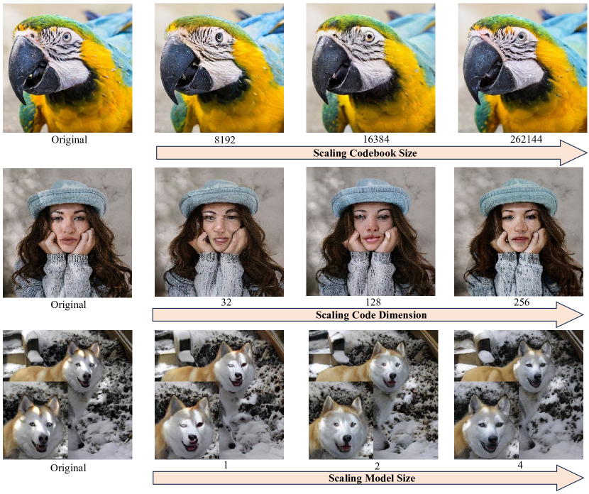
Figure 5: Scaling up visual tokenizers (e.g., codebook size, code dimension and model size) improves visual soundness of reconstruction. Zoom in for a better view.

Type	Model	#Para.	FID$\downarrow$	IS$\uparrow$	Precision$\uparrow$	Recall$\uparrow$
Diffusion	ADM [5]	554M	10.94	101.0	0.69	0.63
	CDM [8]	$-$	4.88	158.7	$-$	$-$
	LDM-4 [20]	400M	3.60	247.7	$-$	$-$
	DiT-XL/2 [18]	675M	2.27	278.2	0.83	0.57
VAR	VAR-d16 [25]	310M	3.30	274.4	0.84	0.51
	VAR-d20 [25]	600M	2.57	302.6	0.83	0.56
	VAR-d24 [25]	1.0B	2.09	312.9	0.82	0.59
	VAR-d30 [25]	2.0B	1.92	323.1	0.82	0.59
MAR	MAR-B [14]	208M	2.31	281.7	0.82	0.57
	MAR-L [14]	479M	1.78	296.0	0.81	0.60
	MAR-H [14]	943M	1.55	303.7	0.81	0.62
AR	VQGAN [6]	227M	18.65	80.4	0.78	0.26
	VQGAN [6]	1.4B	15.78	74.3	$-$	$-$
	VQGAN-re [6]	1.4B	5.20	280.3	$-$	$-$
	ViT-VQGAN [31]	1.7B	4.17	175.1	$-$	$-$
	ViT-VQGAN-re [31]	1.7B	3.04	227.4	$-$	$-$
	RQTran. [13]	3.8B	7.55	134.0	$-$	$-$
	RQTran.-re [13]	3.8B	3.80	323.7	$-$	$-$
	LlamaGen-L [24]	343M	3.80	248.28	0.83	0.51
	LlamaGen-XL [24]	775M	3.39	227.08	0.81	0.54
	LlamaGen-XXL [24]	1.4B	3.09	253.61	0.83	0.53
	LlamaGen-3B [24]	3.1B	3.06	279.72	0.84	0.53
	LlamaGen-L∗ [24]	343M	3.07	256.06	0.83	0.52
	LlamaGen-XL∗ [24]	775M	2.62	244.08	0.80	0.57
	LlamaGen-XXL∗ [24]	1.4B	2.34	253.90	0.80	0.59
	LlamaGen-3B∗ [24]	3.1B	2.18	263.33	0.81	0.58
	Open-MAGVIT2-B [16]	343M	3.08	258.26	0.85	0.51
	Open-MAGVIT2-L [16]	804M	2.51	271.70	0.84	0.54
	Open-MAGVIT2-XL [16]	1.5B	2.33	271.77	0.84	0.54
AR	IBQ-B (Ours)	342M	2.88	254.73	0.84	0.51
	IBQ-L (Ours)	649M	2.45	267.48	0.83	0.52
	IBQ-XL (Ours)	1.1B	2.14	278.99	0.83	0.56
	IBQ-XXL (Ours)	2.1B	2.05	286.73	0.83	0.57

Table 7: Class-conditional generation on $256\times 256$ ImageNet. $*$ specifies the generated images are $384\times 384$ and are resized to 256×256 for evaluation. The evaluation protocol and implementation are the same with ADM.

4.1 Datasets and Metrics

The training of the visual tokenizer and autoregressive transformer are both on $256\times 256$ ImageNet [4]. For visual reconstruction, the reconstruction-FID, denoted as rFID [7], codebook utilization, and LPIPS [34] on ImageNet 50k validation set are adopted to measure the quality of reconstructed images. For visual generation, we measure the quality of image generation by the prevalent metrics FID, IS [21] and Precision/Recall [12].

4.2 Implementations Details

Visual Reconstruction Setup.

We adopt the same model architecture proposed in VQGAN [6]. The visual tokenizer is trained with the following settings: an initial $1e-4$ learning rate with $0.01$ multi-step decay mechanism, an Adam Optimizer [11] with $\beta_{1}=0.5$, $\beta_{2}=0.9$, a total $256$ batch size with $330$ epochs, a combination of reconstruction, GAN [10], perceptual [34], commitment [6], entropy [32], double quantization losses, and LeCAM regularization [27] for training stability. When not specified, we use 16,384 codebook size, 256 code dimension, and 4 ResBlocks as our default tokenizer setting.

Visual Generation Setup.

It is anticipated that the plain autoregressive visual generation method can well exhibit the effectiveness of our visual tokenizer design. Specifically, we adopt Llama-based architecture where the RoPE [23], SwiGLU [22], and RMSNorm [35] techniques are incorporated. We further introduce AdaLN [18] for better visual synthesis quality. The class embedding serves as the start token and the conditional of AdaLN simultaneously. IBQ with width $w$, depth $d$ and head $h$ follows the scaling rules proposed in [24, 25], which is formulated as:

$$w=64d,\quad h=d.$$ (12)

All models are trained with similar settings: a base learning rate of $1e-4$ per $256$ batch size, an AdamW optimizer [15] with $\beta_{1}=0.9$, $\beta_{2}=0.95$, weight decay = $5e-2$, a total $768$ batch size and 300 $\sim$ 450 training epochs corresponding the model size, gradient clipping of $1.0$, and $0.1$ dropout rate for input embedding, FFN module and conditional embedding.

4.3 Main Results

Visual Reconstruction.

Tab. 1 shows the quantitative reconstruction comparison between IBQ and prevalent visual tokenizers. It can be seen that a significant drop in codebook usage on existing VQ methods when scaling codebook size (e.g., VQGAN [6] has a 44% usage for 1024 codebook size, while a 5.9% usage for 16,384 codebook size.), and code dimension (e.g., LlamaGen [24] has a 97% usage for 8-dimension codes, while a 0.29% usage for 256-dimension codes.) Therefore, the actual representational capacity is limited by the codebook collapse.

In contrast, our joint optimization of all codebook embedding and the visual encoder ensures the consistent distribution between them, facilitating the stable training of an large codebook size and embedding visual tokenizer with high utilization. Specifically, IBQ with 16,384 codebook size and 256 code dimension achieves 1.37 rFID, exceeding other VQ methods under the same downsampling rate and codebook size. By increasing the codebook size to 262,144, IBQ outperforms Open-MAGVIT2 [16] and achieves state-of-the-art reconstruction performance (1.00 rFID). We also perform a qualitative comparison with several representative VQ methods in Fig. 4. IBQ exhibits better visual soundness on complex scenarios such as faces and characters.

Visual Generation.

In Tab. 7, we compare IBQ with other generative models, including Diffusion models, AR models, and variants of AR models (VAR [25] and MAR [14]) on class-conditional image generation task. With the powerful visual tokenizers of IBQ, our models show consistent improvements when scaling up the model size (from 300M to 2.1B), and outperform all previous vanilla autoregressive models at different scales of model size. Moreover, IBQ outperforms the diffusion-based model DiT [18], and achieves comparable results with the variants of AR models. These AR model variants focus on the architecture designs of transformers in the second stage, while our work is devoted to better visual tokenizers in the first stage. Therefore, we believe that with our stronger tokenizers, the AR models and their variants can be boosted further.

4.4 Scaling Up IBQ

Existing VQ methods struggle to scale up due to the codebook collapse. For example, the usage and rFID of LlamaGen[24] significantly drop when increasing the code dimension from 8 to 256 (97% $\rightarrow$0.29%, 2.19 rFID$\rightarrow$9.21 rFID), as shown in Tab. 1. This is due to their partial updates during training which progressively widens the distribution gap between non-activated codes and encoded features.

IBQ shows promising scaling capacity in three aspects: 1) Codebook Size: As shown in Tab. 6, there is a significant improvement in reconstruction quality as the codebook size enlarges from 1024 to 16,384. Furthermore, IBQ enables high codebook utilization and consistent gain in visual soundness even training with 262,144 codes. 2) Model Size: Tab. 6 reveals that by extending the number of ResBlock both in the encoder and the decoder, the boost in reconstruction performance can be guaranteed. 3) Code Dimension: interestingly, we observe significant codebook usage increasements when scaling up code dimension. We assume that low-dimensional codes are less discriminative where similar ones tend to be clustered. It indicates that the representative codes are more likely to be selected under our global updating strategy. In contrast, codes with high-dimensional embedding are highly informative since they are mutually sparse in the representation space. Therefore, these codes can be evenly selected during training, which ensures high utilization with better performance. With the above factors, we realize a super large codebook of 262,144 codebook size and 256 dimensions with high codebook usage (84%), achieving the state-of-the-art reconstruction performance (1.00 rFID). To better illustrate the scaling properties, we also provide visualizations in Fig. 5.

4.5 Ablation Studies

Key Designs.

To validate the effectiveness of our method, we conduct ablation studies on several key designs, as shown in Tab. 6. The re-implemented VQGAN performance is 3.98 rFID and 5.3% codebook utilization. Different from previous methods, the replacement from VQ to IBQ achieves consistent distribution between encoded features and the whole codebook by rendering all code differentiable, which brings a clear improvement of both codebook usage (5.3%$\rightarrow$ 98%) and reconstruction quality (3.98 rFID$\rightarrow$1.67 rFID). By incorporating double quantization loss to force the selected code embeddings and encoded visual features toward each other, IBQ guarantees more precise quantization. Following MAGVIT-v2 [32], we enlarge the model size for better compacity, and the reconstruction performance gets improved correspondingly.

Comparison with LFQ.

For fair comparisons, we adopt LFQ [16] with 16,384 codes and replace its asymmetric token factorization with our vanilla transformer architecture. We compare with LFQ on both reconstruction and generation in Tab. 6, and our proposed IBQ performs better, which demonstrates increasing code dimension can improve the reconstruction ability of the visual tokenizer and further boost the visual generation.

5 Conclusion

In this paper, we identify the bottleneck in scaling tokenizers arising from the partial-update strategy in current VQ methods, which progressively broadens the distribution gap between encoded features and non-activated codes, ultimately leading to codebook collapse. To tackle this challenge, we propose a simple yet effective vector quantization method, coined as Index Backpropagation Quantization (IBQ), for scalable tokenizer training, which updates all codes by applying the straight-through estimator on the categorical distribution between visual features and all codebook embeddings, thereby maintaining consistent distribution between the entire codebook and encoded features. Experiments on ImageNet demonstrate that IBQ enables a high-utilization, large-scale visual tokenizer with improved performance in both reconstruction (1.00 rFID) and generation (2.05 gFID), confirming the scalability and effectiveness of our method.

Appendix

Appendix A Autoregressive Model Configurations

We show the detailed autoregressive model configurations in Tab. 8. We scale up the AR models from 342M to 2.1B following the scaling rules proposed in VAR [25].

Appendix B Comparison with Soft Vector Quantization

To comprehensively illustrate the rationality of our IBQ, we compare it with another global update method, Soft Vector Quantization dubbed as Soft VQ. During training, it adopts the weighted average of all code embeddings as the quantized feature $v_{q}$ and incorporates a cosine decay schedule of the temperature ranging from $0.9$ to $1e$-$6$ for one-hot vector approximation. As for inference, it switches back to the original VQGAN way, which selects the code with the highest probability for hard quantization.

As shown in Tab. 9, Soft VQ is far behind IBQ in both reconstruction quality and codebook usage. In the experiments, we observe that the training process of Soft VQ corrupts within a few epochs ($<10$). This may stem from the unstable adversarial training where the adaptive weight of the GAN loss appears enormous and ends up with NAN. In addition, the soft-to-hard manner for one-hot vector approximation brings more difficulty in optimization and incurs inconsistency of quantization between training and inference, as demonstrated by a significant reconstruction quality drop ($16.17\text{rFID}\rightarrow 233.17\text{rFID}$).

Moreover, we provide an in-depth investigation by visualizing the distribution between the codebook and encoded features of Soft VQ. As shown in Fig. 6, although all-code updating strategy is enabled, the inappropriate quantization process tends to cluster codes mistakenly which subsequently suffers from low codebook usage (2.5%). We speculate that the force of the weighted average of code embeddings toward the encoded feature will smooth the codebook representation and result in similar and less informative code embeddings. In contrast, IBQ adopts hard quantization with index backpropagation. The hard quantization only involves the selected codes toward the encoded features for discriminative representation, thus ensuring precise quantization, while index backpropagation performs joint optimization of all codebook and the visual encoder to achieve consistent distribution. Considering the factors above, our proposed IBQ shows dominance in both reconstruction quality and codebook utilization.

Appendix C Additional Visualizations

We provide more qualitative reconstruction and generation samples in Fig. 7 and Fig. 8, respectively.

Appendix D Limitation and Future Work

In this work, we mainly focus on visual tokenizers through scalable training, and adopt vanilla autoregressive transformers for visual generation. We believe that combining our powerful visual tokenizers with advanced AR models is a promising way to improve autoregressive visual generation. In addition, our models are trained on ImageNet [4], limiting the generalization ability. Pretraining tokenizers on more data and training AR models on text-image pairs would be helpful. We leave these for future work.

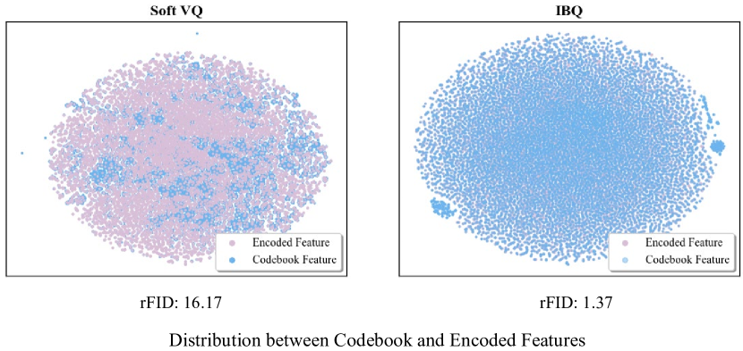
Figure 6: Distribution Gap. The T-SNE results of the codebook (16,384 codebook size and 256 dimension) and sampled encoded features.

Model	Parameters	Width $w$	Head $h$	Depth $d$
IBQ-B	342M	16	16	1024
IBQ-L	649M	20	20	1280
IBQ-XL	1.1B	24	24	1536
IBQ-XXL	2.1B	30	30	1920

Table 8: Model sizes and architecture configurations of IBQ.

Model	Optimization	Training	Inference	rFID$\downarrow$	Usage$\uparrow$
Soft VQ	Corrupted	Soft	Soft	16.17	2.5%
Soft VQ	Corrupted	Soft	Hard	233.17	2.5%
IBQ (Ours)∗	Stable	Hard	Hard	4.03	99%
IBQ (Ours)	Stable	Hard	Hard	1.37	96%

Table 9: Comparison with Soft Vector Quantization. Soft VQ training corrupts after a few epochs. When adopting hard quantization for inference, there is a significant drop in rFID. ^∗ denotes IBQ with the same training epochs as Soft VQ.

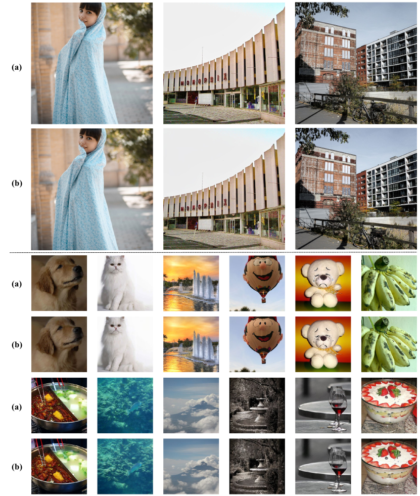
Figure 7: The upper part illustrates the IBQ tokenizer tested at 1024 $\times$ 1024 Unsplash. While the second part showcases the IBQ tokenizer tested at 256 $\times$ 256 Imagenet. (a) indicates the original images and (b) signifies the reconstructions.

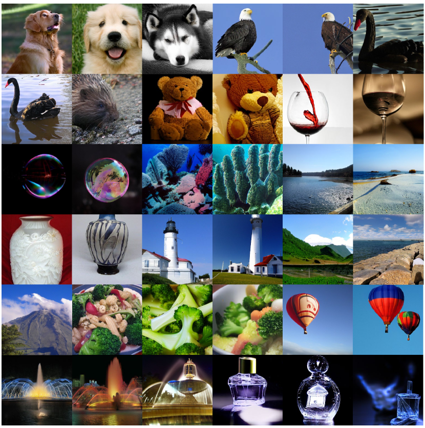
Figure 8: We showcases the 256 $\times$ 256 class conditional generation samples on Imagenet.

References

- Bengio et al. [2013] Yoshua Bengio, Nicholas Léonard, and Aaron Courville. Estimating or propagating gradients through stochastic neurons for conditional computation. arXiv preprint arXiv:1308.3432, 2013.
- Brown et al. [2020] Tom Brown, Benjamin Mann, Nick Ryder, Melanie Subbiah, Jared D Kaplan, Prafulla Dhariwal, Arvind Neelakantan, Pranav Shyam, Girish Sastry, Amanda Askell, Sandhini Agarwal, Ariel Herbert-Voss, Gretchen Krueger, Tom Henighan, Rewon Child, Aditya Ramesh, Daniel Ziegler, Jeffrey Wu, Clemens Winter, Chris Hesse, Mark Chen, Eric Sigler, Mateusz Litwin, Scott Gray, Benjamin Chess, Jack Clark, Christopher Berner, Sam McCandlish, Alec Radford, Ilya Sutskever, and Dario Amodei. Language models are few-shot learners. In NeurIPS, pages 1877–1901, 2020.
- Chang et al. [2022] Huiwen Chang, Han Zhang, Lu Jiang, Ce Liu, and William T. Freeman. Maskgit: Masked generative image transformer. In CVPR, pages 11305–11315, 2022.
- Deng et al. [2009] Jia Deng, Wei Dong, Richard Socher, Li-Jia Li, Kai Li, and Li Fei-Fei. ImageNet: A large-scale hierarchical image database. In CVPR, pages 248–255, 2009.
- Dhariwal and Nichol [2021] Prafulla Dhariwal and Alexander Nichol. Diffusion models beat gans on image synthesis. NeurIPS, 34:8780–8794, 2021.
- Esser et al. [2021] Patrick Esser, Robin Rombach, and Björn Ommer. Taming transformers for high-resolution image synthesis. In CVPR, pages 12873–12883, 2021.
- Heusel et al. [2017] Martin Heusel, Hubert Ramsauer, Thomas Unterthiner, Bernhard Nessler, and Sepp Hochreiter. GANs trained by a two time-scale update rule converge to a local nash equilibrium. In NeurIPS, 2017.
- Ho et al. [2022] Jonathan Ho, Chitwan Saharia, William Chan, David J Fleet, Mohammad Norouzi, and Tim Salimans. Cascaded diffusion models for high fidelity image generation. 23(1):2249–2281, 2022.
- Huang et al. [2023] Mengqi Huang, Zhendong Mao, Zhuowei Chen, and Yongdong Zhang. Towards accurate image coding: Improved autoregressive image generation with dynamic vector quantization. In CVPR, pages 22596–22605, 2023.
- Isola et al. [2017] Phillip Isola, Jun-Yan Zhu, Tinghui Zhou, and Alexei A. Efros. Image-to-image translation with conditional adversarial networks. In CVPR, pages 5967–5976, 2017.
- Kingma [2014] Diederik P Kingma. Adam: A method for stochastic optimization. arXiv preprint arXiv:1412.6980, 2014.
- Kynkäänniemi et al. [2019] Tuomas Kynkäänniemi, Tero Karras, Samuli Laine, Jaakko Lehtinen, and Timo Aila. Improved precision and recall metric for assessing generative models. In NeurIPS, pages 3929–3938, 2019.
- Lee et al. [2022] Doyup Lee, Chiheon Kim, Saehoon Kim, Minsu Cho, and Wook-Shin Han. Autoregressive image generation using residual quantization. In CVPR, pages 11513–11522, 2022.
- Li et al. [2024] Tianhong Li, Yonglong Tian, He Li, Mingyang Deng, and Kaiming He. Autoregressive image generation without vector quantization. arXiv preprint arXiv:2406.11838, 2024.
- Loshchilov [2017] I Loshchilov. Decoupled weight decay regularization. arXiv preprint arXiv:1711.05101, 2017.
- Luo et al. [2024] Zhuoyan Luo, Fengyuan Shi, Yixiao Ge, Yujiu Yang, Limin Wang, and Ying Shan. Open-magvit2: An open-source project toward democratizing auto-regressive visual generation. arXiv preprint arXiv:2409.04410, 2024.
- OpenAI [2023] OpenAI. GPT-4 technical report. arXiv preprint arXiv:2303.08774, 2023.
- Peebles and Xie [2023] William Peebles and Saining Xie. Scalable diffusion models with transformers. In CVPR, pages 4195–4205, 2023.
- Razavi et al. [2019] Ali Razavi, Aaron Van den Oord, and Oriol Vinyals. Generating diverse high-fidelity images with vq-vae-2. In NeurIPS, 2019.
- Rombach et al. [2022] Robin Rombach, Andreas Blattmann, Dominik Lorenz, Patrick Esser, and Björn Ommer. High-resolution image synthesis with latent diffusion models. In CVPR, pages 10684–10695, 2022.
- Salimans et al. [2016] Tim Salimans, Ian Goodfellow, Wojciech Zaremba, Vicki Cheung, Alec Radford, and Xi Chen. Improved techniques for training gans. In NeurIPS, 2016.
- Shazeer [2020] Noam Shazeer. Glu variants improve transformer. arXiv preprint arXiv:2002.05202, 2020.
- Su et al. [2024] Jianlin Su, Murtadha Ahmed, Yu Lu, Shengfeng Pan, Wen Bo, and Yunfeng Liu. Roformer: Enhanced transformer with rotary position embedding, 2024.
- Sun et al. [2024] Peize Sun, Yi Jiang, Shoufa Chen, Shilong Zhang, Bingyue Peng, Ping Luo, and Zehuan Yuan. Autoregressive model beats diffusion: Llama for scalable image generation. arXiv preprint arXiv:2406.06525, 2024.
- Tian et al. [2024] Keyu Tian, Yi Jiang, Zehuan Yuan, Bingyue Peng, and Liwei Wang. Visual autoregressive modeling: Scalable image generation via next-scale prediction. arXiv preprint arXiv:2404.02905, 2024.
- Touvron et al. [2023] Hugo Touvron, Louis Martin, Kevin Stone, Peter Albert, Amjad Almahairi, Yasmine Babaei, Nikolay Bashlykov, Soumya Batra, Prajjwal Bhargava, Shruti Bhosale, Dan Bikel, Lukas Blecher, Cristian Canton-Ferrer, Moya Chen, Guillem Cucurull, David Esiobu, Jude Fernandes, Jeremy Fu, Wenyin Fu, Brian Fuller, Cynthia Gao, Vedanuj Goswami, Naman Goyal, Anthony Hartshorn, Saghar Hosseini, Rui Hou, Hakan Inan, Marcin Kardas, Viktor Kerkez, Madian Khabsa, Isabel Kloumann, Artem Korenev, Punit Singh Koura, Marie-Anne Lachaux, Thibaut Lavril, Jenya Lee, Diana Liskovich, Yinghai Lu, Yuning Mao, Xavier Martinet, Todor Mihaylov, Pushkar Mishra, Igor Molybog, Yixin Nie, Andrew Poulton, Jeremy Reizenstein, Rashi Rungta, Kalyan Saladi, Alan Schelten, Ruan Silva, Eric Michael Smith, Ranjan Subramanian, Xiaoqing Ellen Tan, Binh Tang, Ross Taylor, Adina Williams, Jian Xiang Kuan, Puxin Xu, Zheng Yan, Iliyan Zarov, Yuchen Zhang, Angela Fan, Melanie Kambadur, Sharan Narang, Aurélien Rodriguez, Robert Stojnic, Sergey Edunov, and Thomas Scialom. Llama 2: Open foundation and fine-tuned chat models. arXiv preprint arXiv:2307.09288, 2023.
- Tseng et al. [2021] Hung-Yu Tseng, Lu Jiang, Ce Liu, Ming-Hsuan Yang, and Weilong Yang. Regularizing generative adversarial networks under limited data. In CVPR, pages 7921–7931, 2021.
- Van Den Oord et al. [2017] Aaron Van Den Oord, Oriol Vinyals, et al. Neural discrete representation learning. In NeurIPS, 2017.
- Vaswani et al. [2017] Ashish Vaswani, Noam Shazeer, Niki Parmar, Jakob Uszkoreit, Llion Jones, Aidan N. Gomez, Lukasz Kaiser, and Illia Polosukhin. Attention is all you need. In NeurIPS, pages 5998–6008, 2017.
- Weber et al. [2024] Mark Weber, Lijun Yu, Qihang Yu, Xueqing Deng, Xiaohui Shen, Daniel Cremers, and Liang-Chieh Chen. Maskbit: Embedding-free image generation via bit tokens. arXiv preprint arXiv:2409.16211, 2024.
- Yu et al. [2022] Jiahui Yu, Xin Li, Jing Yu Koh, Han Zhang, Ruoming Pang, James Qin, Alexander Ku, Yuanzhong Xu, Jason Baldridge, and Yonghui Wu. Vector-quantized image modeling with improved VQGAN. In ICLR, 2022.
- Yu et al. [2024a] Lijun Yu, Jose Lezama, Nitesh Bharadwaj Gundavarapu, Luca Versari, Kihyuk Sohn, David Minnen, Yong Cheng, Agrim Gupta, Xiuye Gu, Alexander G Hauptmann, Boqing Gong, Ming-Hsuan Yang, Irfan Essa, David A Ross, and Lu Jiang. Language model beats diffusion - tokenizer is key to visual generation. In ICLR, 2024a.
- Yu et al. [2024b] Qihang Yu, Mark Weber, Xueqing Deng, Xiaohui Shen, Daniel Cremers, and Liang-Chieh Chen. An image is worth 32 tokens for reconstruction and generation. arXiv preprint arXiv:2406.07550, 2024b.
- Zhang et al. [2018] Richard Zhang, Phillip Isola, Alexei A. Efros, Eli Shechtman, and Oliver Wang. The unreasonable effectiveness of deep features as a perceptual metric. In CVPR, pages 586–595, 2018.
- Zhang et al. [2022] Susan Zhang, Stephen Roller, Naman Goyal, Mikel Artetxe, Moya Chen, Shuohui Chen, Christopher Dewan, Mona T. Diab, Xian Li, Xi Victoria Lin, Todor Mihaylov, Myle Ott, Sam Shleifer, Kurt Shuster, Daniel Simig, Punit Singh Koura, Anjali Sridhar, Tianlu Wang, and Luke Zettlemoyer. OPT: open pre-trained transformer language models. arXiv preprint arXiv:2205.01068, 2022.
- Zhu et al. [2024] Lei Zhu, Fangyun Wei, Yanye Lu, and Dong Chen. Scaling the codebook size of vqgan to 100,000 with a utilization rate of 99%. arXiv preprint arXiv:2406.11837, 2024.