Electron Beam Characterization via Quantum Coherent Optical Magnetometry
Abstract
We present a quantum optics-based detection method for determining the position and current of an electron beam. As electrons pass through a dilute vapor of rubidium atoms, their magnetic field perturb the atomic spin’s quantum state and causes polarization rotation of a laser resonant with an optical transition of the atoms. By measuring the polarization rotation angle across the laser beam, we recreate a 2D projection of the magnetic field and use it to determine the e-beam position, size and total current. We tested this method for an e-beam with currents ranging from 30 to 110 A. Our approach is insensitive to electron kinetic energy, and we confirmed that experimentally between 10 to 20 keV. This technique offers a unique platform for non-invasive characterization of charged particle beams used in accelerators for particle and nuclear physics research.
With the advent of charged particle accelerators came the need for accurate beam diagnostics. Driven by improvements to quality and control of charged particle beams, the sensitivity and precision of in-situ diagnostics must meet the needs of new particle accelerators where increasingly strict demands are placed on beam properties such as energy, current, emittance and others. The need for increasingly precise beam diagnostics for a wide range of parameters inspires relentless efforts to continue towards the development of more robust, non-invasive spatial beam parameter measurements. Much of this development is focused on the methods relying on optical signals. Synchrotron radiation has been used for monitoring beam position and size Bossart et al. (1980); Wang et al. (2013); Li et al. (2022), and laserwires Hofmann et al. (2018); Corner et al. (2014) rely on Compton scattering from a high-power laser to extract the charged particle beam parameters. However, these types of optical diagnostics are limited by technical requirements on the particle and laser beams. For example, synchrotron radiation is only available in particle trajectory-bending components such as magnets, while the laserwire method requires a high-intensity laser to slowly scan the beam profile, and often requires additional radiation, or electronic, detectors. Beam profile monitors based on gas ionization and excitation by particle beams have been demonstrated and used at different accelerators Anne et al. (1993); Sandberg et al. (2021); Variola, Jung, and Ferioli (2007). More recently, a 2D beam monitor measuring fluorescence from the interaction between a 5 keV particle beam and a supersonic gas curtain was reported Salehilashkajani et al. (2022), but it is not suitable for spatial longitudinal profile measurement, and the sensitivity is quite limited. It is worth mentioning another type of device widely used in the accelerator community, the RF-based beam monitor, which can provide beam centroid at high resolution, but is incapable of profile measurement Maesaka et al. (2012).
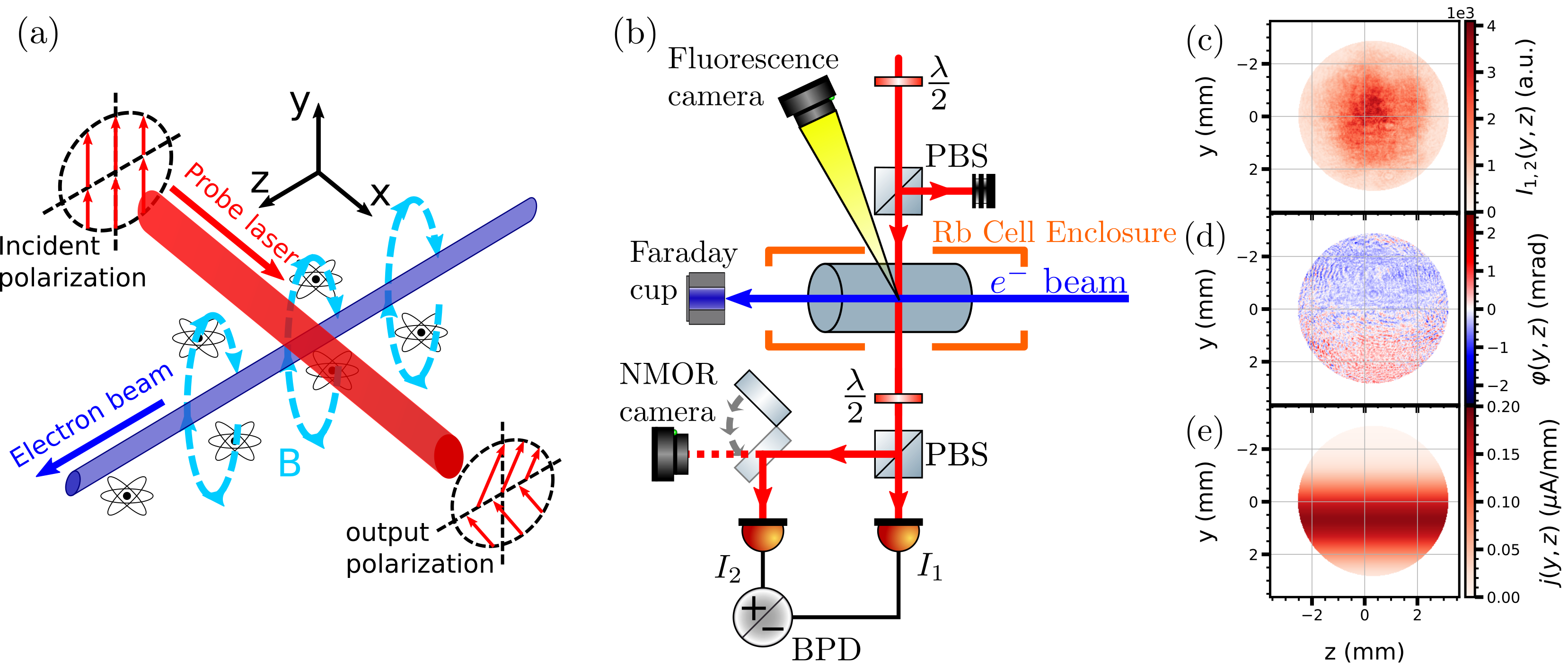
In this paper, we propose a qualitatively different approach to beam diagnostics that takes advantage of recent advances in quantum atom-based optical sensors to map the magnetic field produced by the moving charged particles and then reconstruct the beam parameters. In this proof-of-principle demonstration, we use coupling between resonant laser light and atomic spins to monitor evolution of the latter in the magnetic field of a collimated electron beam. The essence of the proposed approach is shown in Fig. 1(a). The -beam travels through a cell containing a dilute gas of rubidium atoms. Within the cell each Rb spin precesses at a rate determined by the local magnetic field. A linearly polarized laser beam traverses the volume surrounding the charge particle beam and probes the atomic spins: the nonlinear magneto-optical polarization rotation (NMOR) effect Budker and Jackson Kimball (2013); Weis, Bison, and Grujić (2017); Fu et al. (2020) rotates the optical linear polarization axis due to the magnetic field of the -beam. By measuring the polarization rotation variation across the laser beam cross-section, we are able to determine the local magnetic field of the -beam and reconstruct its transverse spatial profile. Our detection scheme is largely non-invasive as the -beam is minimally affected by low-density alkali vapor () localized within a 30 cm region enclosed in high-vacuum111We calculate a Bethe energy loss of 0.1 eV/m at a Rb density of for 20 keV electrons. At 1 GeV, the energy loss is 0.04 eV/m.. The strong resonant coupling between laser light and atomic spin coherence enhances the sensitivity compared to the approaches based on incoherent electron impact-induced fluorescence Salehilashkajani et al. (2022). This demonstration is a stepping stone toward more sensitive and comprehensive detection of charged particle beams using advanced spectroscopy techniques.
The proposed -beam detector relies on two effects: high sensitivity of atomic spin state superposition to the magnetic field and strong dependence of atoms’ resonant optical properties on their spin state. Thanks to the Zeeman effect, the energy sub-levels with different magnetic quantum numbers, , shift by different amounts, a superposition of two such sub-levels evolves in time, developing a magnetic field dependent relative phase. A resonant, and linearly polarized laser field, can simultaneously prepare the desired quantum superposition and measure its evolution. Indeed, the two circularly-polarized components create a two-photon transition between the states with (spin alignment, see Fig. S1 in Supplementary). The optical field’s propagation through the magnetic field changes the relative phase between the two circular polarization components, resulting in rotation of the original linear polarization. This effect, known as nonlinear magneto-optical polarization rotation (NMOR), is a convenient and sensitive method for optical magnetic field measurements. In the case of long spin coherence lifetime and exact optical resonance, the rate at which the polarization rotation angle rotates (as the laser propagates along the -axis) is proportional to the local magnetic field (see Supplementary A for derivation):
| (1) |
where we assume the greatest contribution to is when the probe beam direction and magnetic field are along the -axis; , , and are the wavelength, local intensity, and speed of light, respectively; is the density of the Rb vapor, and Hz/nT is the gyromagnetic ratio for 85Rb atoms. In principle, since the intrinsic spin coherence lifetime is very long, and in some experiments Balabas et al. (2010) was extended up to many seconds, NMOR-based magnetometers can achieve an impressive sub-pT sensitivity Rosner et al. (2022); Lucivero et al. (2021). When the spin decoherence and optical losses are accounted for, the exact proportionality coefficient between the polarization rotation rate and the applied magnetic field is more complex and depends, at some extent, on many experimental parameters (lifetimes of both optical spin states, laser frequency detuning from the optical resonance, influence of additional near-resonant atomic levels, etc. See Supplementary A for detailed derivations). We experimentally derive the rotation response profile across the Gaussian laser beam by applying a known constant magnetic field and measure the polarization rotation for each camera pixel.
In the experiment, the laser beam propagates along the -axis shown in Fig. 1(a), nearly perpendicular to the electron beam direction, designated as the -direction. The laser is linearly polarized in the -direction, perpendicular to both the electron and the laser beam propagation directions. In this configuration, the laser polarization rotation should only be sensitive to the longitudinal magnetic field component (Faraday configuration) Budker et al. (2002). For a narrow laser beam the magnitude and sign of the rotation angle depend on the cumulative magnetic field along the optical propagation path. Thus, imaging a 2D map of the polarization angle on a camera using a laser beam with large cross-section, we can in principle obtain a transverse profile of the -beam. The schematic of the experimental setup is shown in Fig. 1(b).
We used a commercial thermionic electron source generating a collimated electron beam with energy 10-20 keV and current up to 200 A. The electron beam passes through a glass cell (inner dimensions: 10 mm 10 mm 45 mm) containing rubidium vapor before terminating in a Faraday cup. Differential pumping through 8 mm apertures, up- and down-stream of the cell, are used to confine the vapor to the cell and to keep it at constant pressure. The vapor was maintained at C, corresponding to a 85Rb vapor density of and a pressure of Torr, housed within a vacuum system of pressure nTorr during experiment operation to preserve the quality of the electron source filament. Since such system is most sensitive to small magnetic fields, so we suppress environmental fields by placing the atomic vapor inside a layer of -metal magnetic shielding, and use external coils to further reduce the background magnetic fields.
For optical detection, we use an external cavity diode laser (ECDL) operating at the line of 85Rb (wavelength nm), specifically at the transition. The laser beam was linearly polarized using a polarizing beam splitter (PBS) cube and enlarged to 6 mm before the entering the Rb-filled glass cell to capture the full -beam diameter. Beyond the cell, the laser polarization rotation is analyzed using a balanced polarimeter, consisting of a half-wave plate that rotates the polarization by , an analyzer PBS and a differential amplified photodetector (BPD). In the absence of the -beam, the intensities of the two PBS outputs are balanced. A small rotation of the polarization produces a proportional variation between the two channel intensities, allowing accurate calculations of :
| (2) |
In our experiment we measure total power changes in each channel that let us measure the integrated rotation signal, which is convenient for system alignment. For most presented data we use a CCD-based imaging system (magnification 0.50) to record the spatial distribution across the laser beam. To ensure the consistency between the recorded intensity masks they are recorded consecutively at the same camera position, but with a different angle of the waveplate before the polarizer. An example of such intensity profile for one of the channels is shown in Fig. 1(c), in which the intensity difference between two channels, induced by the -beam, is not distinguishable by the naked eye. As the laser beam has Gaussian intensity profile, we only use its central part with sufficient intensity in further calculations. In addition, the electron beam was pulsed on and off at Hz to record two consecutive images, with and without the -beam. Subtracting the images from each other allows us to remove any residual polarization rotation due to stray magnetic fields or optical elements to ensure that we only detect the polarization rotation caused by the -beam.
By capturing the intensity profiles of the two outputs on a CCD camera with two waveplate positions, we were able to calculate local variations of within the laser beam cross-section as shown in Fig. 1(d). The angle distribution within the laser beam is extracted by applying Eq. 2 to each camera pixel. Since the -beam generates a circulating magnetic field in plane, and the nonlinear polarization rotation is primarily sensitive to the component of the magnetic field, we expect to see a sign change in the measured polarization rotation angle below and above the center of the -beam, as shown in Fig. 1(a).

To obtain more quantitative information about the -beam, we assume that its current density is cylindrically symmetric and has a Gaussian transverse profile:
| (3) |
where is the total current, and is the beam half-width. The corresponding magnetic field maintains cylindrical symmetry, forming concentric field lines around the beam central axis, and its magnitude can be easily found using Ampere’s law:
| (4) |
where is the permeability of free space.
In the limit of a weak magnetic field, the total measured polarization rotation is integrated along the laser probe propagation path :
| (5) |
Here we assume that the rotation angle is small, the -beam is collimated and its magnetic field has no -dependence. In this case any changes in the polarization rotation in this direction can only be caused by the variation in the atomic response due to, e.g., laser intensity variation. Using Eq. 4, and assuming that the length of the cell is much larger than the -beam width , we can find an analytical expression for the polarization rotation for an electron beam centered at vertical location :
| (6) |
where is the error function, and we assume . For a longer cell the first term dominates the rotation, while the edge effects become more noticeable farther from the -beam center.
It is convenient to introduce a normalized signal since it depends only on the -beam current distribution. For a Gaussian current distribution, according to Eq. 6, the normalized signal is an error function, centered at the vertical position of the -beam , and the maximum variation of depends only on the total -beam current, that allows for robust measurements of these parameters even for a noisy signals. An example of the electron current distribution using the parameters obtained from fitting the normalized rotation spectra are shown in Fig. 1(e).
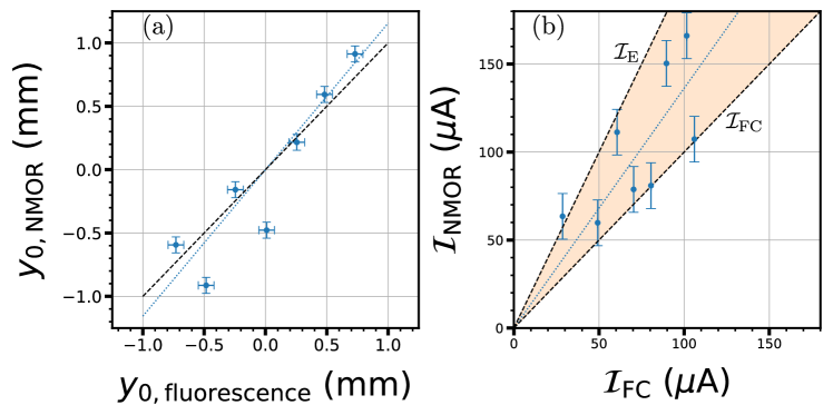
Fig. 2 shows the examples of the recorded normalized signal for two positions of the -beam. As expected, the polarization rotation changes direction from positive to negative at the -beam center position, and the signal is uniform in the -direction. To obtain the -beam parameters we fit the 2D experimental signal distribution with the error function. We then repeated the measurements for varied electron beam positions and values of the total current, as shown in Fig. 3. We verify the accuracy of the beam position measurements by capturing images of fluorescence from Rb atoms ionized by the -beam (see Supplementary C for details). While both signals are noisy, the measured centroid position variation matches within 16% between the two methods, indicating that the spatial coordinate systems agree between the two separate imaging systems. Similarly, we compare the total -beam current value extracted from the polarization rotation measurements with that measured at the Faraday cup and electron emission current , located approximately 25 cm downstream of the Rb cell, matching within 36% of and 14% of between the two methods. Varying the electron beam energy between 10 to 20 keV yielded no significant changes in the profiles or quantities derived using the polarization rotation method.
From the fit, we obtain a FWHM -beam diameter of mm. Although we are unable to independently verify the precise profiles of the electron beam, this value is noticeably broader than that obtained from the fluorescence fits, mm FWHM. The uncertainty for these quantities are derived by considering the variance of the profile parameters of the datasets. We attribute this discrepancy between the widths in part to poor signal-to-noise ratio (SNR) of the rotation signal, especially at the edges of the laser beam, where the laser intensity is low. The overall rotation signal was typically below 1 mrad, and thus strongly affected by the camera electronic noise. Further, the presence of a transverse magnetic field has been shown to broaden the NMOR resonance Anisimov et al. (2003), and thus the unaccounted transverse components of the magnetic field can increase the estimated width of the electron beam. In the future we plan improve the accuracy of the electron beam width measurements by, for example, realizing a more complex optical interrogation scheme to enhance atomic spin coherence and boost the magnetic response of atoms Zhou et al. (2018); Zhu et al. (2021), as well as by developing a model describing the polarization rotation for arbitrary magnetic field orientation. Also, using a low-noise CCD camera and pulsing the -beam at higher rate will remove the dominant source of the technical noise and may boost the sensitivity by several order of magnitude, limited by the laser shot noise (see Supplementary B for details). Moreover, in this case, we may be able further improve the performance by using a non-classical (squeezed) optical field Wolfgramm et al. (2010); Horrom et al. (2012); Otterstrom, Pooser, and Lawrie (2014); Bai et al. (2021); Li and Novikova (2022); Wu et al. (2023). The ultimate spatial resolution of our method is diffraction limited and can potentially resolve details down to a few microns. Using these enhancements, we can accurately image the current distribution of the electron beam non-invasively with optimum SNR.
Looking forward, higher sensitivity and spatial resolution could be achieved by employing advanced spectroscopic methods based on two or more lasers. For example, the 2D transverse current distribution can potentially be mapped out by 4-wave mixing, in which two intersecting probe lasers generate a third beam (imaged on a camera) that depends on the magnetic field in the crossing region Boyer et al. (2007). Currently we are investigating 2- and 3-photon excitation to Rydberg states where we expect much higher sensitivity to the magnetic and electric fields from the -beam due to their large Stark and Zeeman shifts Thaicharoen et al. (2019); Dietsche et al. (2019). Indeed, Rydberg states of ultracold atoms may have sufficient sensitivity for single particle detection Jerkins et al. (2010); Kawasaki (2023).
In summary, thanks to nonlinear interaction with atomic spins, the light polarization rotates in a dilute alkali-metal vapor in the presence of the magnetic field produced by a passing charged particle beam. Taking advantage of this effect, we demonstrated a non-invasive method for characterizing the position and total current of an electron beam that was obtained by mapping the nonlinear polarization rotation of a transverse probe laser crossing the -beam. We experimentally evaluated the accuracy of the proposed technique to determine the total current and transverse position at 20 keV for -beam currents between 30–110 A, and discussed its current limitations. Since the -beam is detected via its magnetic field, the scheme is insensitive to the beam energy Ramaswamy and Malinovskaya (2022), charged particle type and local electric fields associated with the beam. We expect that this technique can be applied to high energy particle accelerators and also refined to meet the precision required for experiments at the frontier of nuclear and high-energy physics research.
Supplementary Material
See the supplementary material for detailed discussion of NMOR, sensitivity, and electron-induced rubidium fluorescence.
Acknowledgements.
This work is supported by U.S. DOE Contract No. DE-AC05-06OR23177, NSF award 2326736 and Jefferson Lab LDRD program. The collaboration thanks Jiahui Li and Cutter Fugett for their assistance in the early stages of the project.Data Availability Statement
The data that support the findings of this study are available from the corresponding author upon reasonable request.
References
References
- Bossart et al. (1980) R. Bossart, J. Bosser, L. Burnod, E. d’Amico, G. Ferioli, J. Mann, F. Meot, and R. Coïsson, “Proton beam profile monitor using synchrotron light,” in 11th International Conference on High-Energy Accelerators: Geneva, Switzerland, July 7–11, 1980, edited by W. S. Newman (Birkhäuser Basel, Basel, 1980) pp. 470–475.
- Wang et al. (2013) S. Wang, D. Rubin, J. Conway, M. Palmer, D. Hartill, R. Campbell, and R. Holtzapple, “Visible-light beam size monitors using synchrotron radiation at cesr,” Nuclear Instruments and Methods in Physics Research Section A: Accelerators, Spectrometers, Detectors and Associated Equipment 703, 80–90 (2013).
- Li et al. (2022) W. Li, J. Yan, P. Liu, and Y. K. Wu, “Synchrotron radiation interferometry for beam size measurement at low current and in large dynamic range,” Phys. Rev. Accel. Beams 25, 080702 (2022).
- Hofmann et al. (2018) T. Hofmann, G. Boorman, A. Bosco, S. Gibson, and F. Roncarolo, “A low-power laserwire profile monitor for h- beams: Design and experimental results,” Nuclear Instruments and Methods in Physics Research Section A: Accelerators, Spectrometers, Detectors and Associated Equipment 903, 140–146 (2018).
- Corner et al. (2014) L. Corner, A. Aryshev, G. Blair, S. Boogert, P. Karataev, K. Kruchinin, L. Nevay, N. Terunuma, J. Urakawa, and R. Walczak, “Laserwire: A high resolution non-invasive beam profiling diagnostic,” Nuclear Instruments and Methods in Physics Research Section A: Accelerators, Spectrometers, Detectors and Associated Equipment 740, 226–228 (2014), proceedings of the first European Advanced Accelerator Concepts Workshop 2013.
- Anne et al. (1993) R. Anne, Y. Georget, R. Hue, C. Tribouillard, and J. Luc Vignet, “A noninterceptive heavy ion beam profile monitor based on residual gas ionization,” Nuclear Instruments and Methods in Physics Research Section A: Accelerators, Spectrometers, Detectors and Associated Equipment 329, 21–28 (1993).
- Sandberg et al. (2021) H. Sandberg, W. Bertsche, D. Bodart, S. Gibson, S. Jensen, S. Levasseur, K. Satou, G. Schneider, J. Storey, and R. Veness, “Commissioning of timepix3 based beam gas ionisation profile monitors for the CERN proton synchrotron.” JACoW IBIC 2021, 172–175 (2021).
- Variola, Jung, and Ferioli (2007) A. Variola, R. Jung, and G. Ferioli, “Characterization of a nondestructive beam profile monitor using luminescent emission,” Phys. Rev. ST Accel. Beams 10, 122801 (2007).
- Salehilashkajani et al. (2022) A. Salehilashkajani, H. D. Zhang, M. Ady, N. Chritin, P. Forck, J. Glutting, O. R. Jones, R. Kersevan, N. Kumar, T. Lefevre, T. Marriott-Dodington, S. Mazzoni, I. Papazoglou, A. Rossi, G. Schneider, O. Sedlacek, S. Udrea, R. Veness, and C. P. Welsch, “A gas curtain beam profile monitor using beam induced fluorescence for high intensity charged particle beams,” Applied Physics Letters 120, 174101 (2022).
- Maesaka et al. (2012) H. Maesaka, H. Ego, S. Inoue, S. Matsubara, T. Ohshima, T. Shintake, and Y. Otake, “Sub-micron resolution rf cavity beam position monitor system at the sacla xfel facility,” Nuclear Instruments and Methods in Physics Research Section A: Accelerators, Spectrometers, Detectors and Associated Equipment 696, 66–74 (2012).
- Budker and Jackson Kimball (2013) D. Budker and D. F. Jackson Kimball, eds., Optical Magnetometry (Cambridge University Press, Cambridge, 2013).
- Weis, Bison, and Grujić (2017) A. Weis, G. Bison, and Z. D. Grujić, “Magnetic resonance based atomic magnetometers,” in High Sensitivity Magnetometers. Smart Sensors, Measurement and Instrumentation, Vol. 19, edited by A. Grosz, M. Haji-Sheikh, and S. Mukhopadhyay (Springer, Cham, 2017) pp. 361–424.
- Fu et al. (2020) K. M. C. Fu, G. Z. Iwata, A. Wickenbrock, and D. Budker, “Sensitive magnetometry in challenging environments,” AVS Quantum Science 2, 044702 (2020).
- Note (1) We calculate a Bethe energy loss of 0.1 eV/m at a Rb density of for 20 keV electrons. At 1 GeV, the energy loss is 0.04 eV/m.
- Balabas et al. (2010) M. V. Balabas, T. Karaulanov, M. P. Ledbetter, and D. Budker, “Polarized alkali-metal vapor with minute-long transverse spin-relaxation time,” Phys. Rev. Lett. 105, 070801 (2010).
- Rosner et al. (2022) M. Rosner, D. Beck, P. Fierlinger, H. Filter, C. Klau, F. Kuchler, P. Rößner, M. Sturm, D. Wurm, and Z. Sun, “A highly drift-stable atomic magnetometer for fundamental physics experiments,” Applied Physics Letters 120, 161102 (2022).
- Lucivero et al. (2021) V. G. Lucivero, W. Lee, N. Dural, and M. V. Romalis, “Femtotesla direct magnetic gradiometer using a single multipass cell,” Physical Review Applied 15, 014004 (2021).
- Budker et al. (2002) D. Budker, W. Gawlik, D. F. Kimball, S. M. Rochester, V. V. Yashchuk, and A. Weis, “Resonant nonlinear magneto-optical effects in atoms,” Rev. Mod. Phys. 74, 1153 (2002).
- Anisimov et al. (2003) P. M. Anisimov, R. A. Akhmedzhanov, I. V. Zelensky, and E. A. Kuznetsova, “Influence of transverse magnetic fields and depletion of working levels on the nonlinear resonance faraday effect,” Journal of Experimental and Theoretical Physics 97, 868–874 (2003).
- Zhou et al. (2018) F. Zhou, E. Y. Zhu, Y. L. Li, E. W. Hagley, and L. Deng, “Nanotesla-level, shield-less, field-compensation-free, wave-mixing-enhanced body-temperature atomic magnetometry for biomagnetism,” (2018).
- Zhu et al. (2021) C. J. Zhu, J. Guan, F. Zhou, E. Y. Zhu, and Y. Li, “Giant magneto-optical rotation effect in rubidium vapor measured with a low-cost detection system,” OSA Continuum 4, 2527–2534 (2021).
- Wolfgramm et al. (2010) F. Wolfgramm, A. Cerè, F. A. Beduini, A. Predojević, M. Koschorreck, and M. W. Mitchell, “Squeezed-light optical magnetometry,” Physical Review Letters 105, 053601 (2010).
- Horrom et al. (2012) T. Horrom, R. Singh, J. P. Dowling, and E. E. Mikhailov, “Quantum-enhanced magnetometer with low-frequency squeezing,” Physical Review A - Atomic, Molecular, and Optical Physics 86, 023803 (2012).
- Otterstrom, Pooser, and Lawrie (2014) N. Otterstrom, R. C. Pooser, and B. J. Lawrie, “Nonlinear optical magnetometry with accessible in situ optical squeezing,” Opt. Lett. 39, 6533–6536 (2014).
- Bai et al. (2021) L. Bai, X. Wen, Y. Yang, L. Zhang, J. He, Y. Wang, and J. Wang, “Quantum-enhanced rubidium atomic magnetometer based on faraday rotation via 795 nm stokes operator squeezed light,” Journal of Optics 23, 085202 (2021).
- Li and Novikova (2022) J. Li and I. Novikova, “Improving sensitivity of an amplitude-modulated magneto-optical atomic magnetometer using squeezed light,” J. Opt. Soc. Am. B 39, 2998–3003 (2022).
- Wu et al. (2023) S. Wu, G. Bao, J. Guo, J. Chen, W. Du, M. Shi, P. Yang, L. Chen, and W. Zhang, “Quantum magnetic gradiometer with entangled twin light beams,” Science Advances 9, eadg1760 (2023).
- Boyer et al. (2007) V. Boyer, C. F. McCormick, E. Arimondo, and P. D. Lett, “Ultraslow propagation of matched pulses by four-wave mixing in an atomic vapor,” Phys. Rev. Lett. 99, 143601 (2007).
- Thaicharoen et al. (2019) N. Thaicharoen, K. R. Moore, D. A. Anderson, R. C. Powel, E. Peterson, and G. Raithel, “Electromagnetically induced transparency, absorption, and microwave-field sensing in a rb vapor cell,” Phys. Rev. A 100, 063427 (2019).
- Dietsche et al. (2019) E. K. Dietsche, A. Larrouy, S. Haroche, J. M. Raimond, M. Brune, and S. Gleyzes, “High-sensitivity magnetometry with a single atom in a superposition of two circular rydberg states,” Nature Phys. 15, 326 (2019).
- Jerkins et al. (2010) M. Jerkins, J. P. Klein, J. H. Majors, F. Robicheaux, and M. G. Raizen, “Using cold atoms to measure neutrino mass,” New J. Phys. 12, 043022 (2010).
- Kawasaki (2023) A. Kawasaki, “Tracking a nonrelativistic charge with an array of rydberg atoms,” Phys. Rev. Res. 5, 043178 (2023).
- Ramaswamy and Malinovskaya (2022) A. Ramaswamy and S. A. Malinovskaya, “Control with eit: High energy charged particle detection,” in Progress in Nanoscale and Low-Dimensional Materials and Devices: Properties, Synthesis, Characterization, Modelling and Applications, edited by H. Ünlü and N. J. M. Horing (Springer International Publishing, Cham, 2022) pp. 363–392.