\svgsetup

inkscapelatex=false

The asymptotic behavior of attention in transformers

Á. Rodríguez Abella, J.P. Silvestre, P. Tabuada Electrical and Computer Engineering Department
University of California at Los Angeles
rodriguezabella@g.ucla.edu, joaosilvestre@g.ucla.edu, tabuada@ee.ucla.edu
Abstract.

A key component of transformers is the attention mechanism orchestrating how each token influences the propagation of every other token through a transformer. In this paper we provide a rigorous, mathematical analysis of the asymptotic properties of attention in transformers. Although we present several results based on different assumptions, all of them point to the same conclusion, all tokens asymptotically converge to each other, a phenomenon that has been empirically reported in the literature. Our findings are carefully compared with existing theoretical results and illustrated by simulations and experimental studies using the GPT-2 model.

1. Introduction

The incorporation of attention [1] in natural language processing was a significant breakthrough, particularly in the context of sequence-to-sequence models, enabling the creation of transformers [2] which revolutionized the field. Even initial transformer models such as GPT [3] or Bert [4] showed drastic improvements over previous approaches such as the Long Short-Term Memory model [5].

As practical applications of deep neural networks, such as image recognition [6], natural language processing [7], and autonomous driving [8], continue to advance, our understanding of these networks is struggling to keep pace [9]. This underscores the critical importance of our study, which aims to delve deeper into transformers and their dynamics. Our understanding of transformers is currently limited by their inherent complexity, making it challenging to comprehensively explain their behavior [10]. However, recent studies have shown the emergence of clusters of tokens empirically and theoretically [11; 12; 13; 14]. These findings suggest that without proper care, large transformers may collapse, a phenomenon where the tokens cluster, limiting the model’s ability to produce different outputs.

Our work was motivated by the paper [15] where a mathematical model for attention was proposed, based on prior work on similar models [16; 17], and investigated. The authors share the vision outlined in [15], a better understanding of the role and importance of attention mechanisms can be achieved through the study of mathematical models. Our contribution lies in bringing ideas developed by the control community, where the study of asymptotic properties of dynamical and control systems is a central preoccupation, to bear on this problem. While deferring to the next section a more detailed comparison between our results and those available in the literature, we emphasize here that, in contrast with [15; 13; 14], we do not rely on stochastic and/or mean-field techniques and rather adopt a geometric perspective drawing from control theory, e.g., from consensus dynamics on manifolds [18] such as spheres  [19; 20] and Input-to-State Stability [21; 22; 23].

Contributions and plan of the paper

The main contribution of this work is to provide a number of results, for a differential equation model of attention, showing that all tokens converge to a single cluster thereby leading to a collapse of the model. We use the term consensus equilibria to refer to such clusters as is done in the consensus literature [24; 25]. These results hold under different assumptions on the parameters of the model —namely, the query ($Q$), key ($K$) and value matrices ($U$), as well as the number of heads ($h$)— that are summarized in Table 1. More specifically, the paper is organized as follows:

  • In Section 2 we introduce the differential equation model for attention studied in this paper. Since layer normalization is part of the model, tokens will evolve on ellipsoids. As we are mainly concerned with attention, the model does not describe the effect of feedforward layers111By feedforward layer we mean the layer implementing a perceptron, i.e., an elementwise activation function acting on an affine function of the input, see, e.g., [26]. in a transformer. Yet, we briefly discuss how the model can be extended to accommodate feedforward layers and the challenges brought by such extension.

  • Section 3 is devoted to the single-head case with $U$ being the identity and $P=Q^{\top}\,K$ being time invariant, positive definite, and symmetric. With Theorem 3.2, we prove that the dynamics of the transformer is a Riemannian gradient vector field, from which we conclude convergence to an equilibrium point (guaranteed to be of consensus type when $P$ is the identity) for every initial position of the tokens. Although the gradient nature of the dynamics, in this case, was already observed and exploited in [15], for the benefit of the readers we provide a formal proof of this fact in a slightly more general setting.

  • In Section 4 we show that tokens converge to a consensus equilibrium whenever their starting positions lie in the interior of some hemisphere of the ellipsoid. This is stated in Theorem 4.1, which holds for any number of heads and time varying matrix $P=Q^{\top}\,K$ provided that $U$ is the identity and $P$ is bounded and uniformly continuous as a function of the time. A similar result is reported in [15] under Lemma 4.2. However, its conclusions hold under the stronger assumptions that both $U$ and $P=Q^{\top}K$ are the identity matrix and there is a single attention head.

The previous results hold under no assumptions on the attention matrix other those induced by the assumptions on $P$. In the next sections, we focus on the auto-regressive case, also known as causal attention, where the self-attention matrix is lower triangular.

  • For the auto-regressive case with $U$ being the identity, the first token is fixed. In Section 5, we show that all tokens converge to the position of the first one for almost every initial position of the tokens. In fact, Theorem 5.1 ensures asymptotic stability of this consensus equilibrium. This holds for any number of heads and any time varying $P$ matrix provided it is bounded. Similar conclusions are reported under Theorem 4.1 in [27] by imposing stronger assumptions: time invariance of $P=Q^{\top}K$ and existence of a single attention head.

  • To conclude the theoretical part, Section 6 extends the previous result to the case where $U$ is a time invariant symmetric matrix and the multiplicity of its largest eigenvalue is one. Therefore, the corresponding eigenspace divides the sphere in two different hemispheres. Theorem 6.1 ensures that the tokens will converge to a consensus equilibrium (moreover, that equilibrium is asymptotically stable) if all the tokens start in one of those hemispheres. We were only able to establish this result for the single-head case although we believe it holds in greater generality. To the best of the author’s knowledge there is no result available in the literature for the case where $U$ is not the identity matrix although this is conjectured, but not proved, in [27].

  • In Section 7 we illustrate the theoretical results through simulations of the mathematical model for attention. We do this using a small number of tokens in low dimensions, for better visualization, as well as a number of tokens and dimension comparable to what is used in the GPT-2 model. We also report on several experiments with the GPT-2 model suggesting convergence to a consensus equilibria in more general situations than those captured by our theoretical results thus providing additional confirmation for model collapse.

Full attention Causal attention (auto-regressive)
Section §3 §4 §5 §6
# of heads $h=1$ $h\geq 1$ $h\geq 1$ $h=1$
$P(t)=Q(t)^{\top}\,K(t)$ Time invariant, symmetric, positive definite Time varying, uniformly continuous, bounded Time varying, bounded Time varying, bounded
$U(t)$ Identity Identity Identity Time invariant, symmetric
Result Theorem 3.2 Theorem 4.1 Theorem 5.1 Theorem 6.1
Statement Gradient flow, convergence to equilibrium Convergence to consensus Asympt. stability of consensus (determined by the first token) Asympt. stability of consensus (determined by eigenspace of largest eigenvalue of $U$)
Domain of attraction Whole sphere Some hemisphere Conull (complement of zero measure) Fixed hemisphere
Table 1. Summary of the results presented in this work for several particular cases of the continuous model (7), where $Q(t)$, $K(t)$, and $U(t)$ denote the query, key and value matrices, respectively.

Notations

We use the letters $n,\ell,r$ and $s$ to denote natural numbers, i.e., elements of $\mathbb{N}=\{1,2,\ldots\}$. The space of $r\times s$ real matrices is denoted by $\mathcal{M}_{r\times s}(\mathbb{R})$. In particular, $\mathbb{I}_{r}\in\mathcal{M}_{r\times r}(\mathbb{R})$ denotes the identity matrix. The elements of $\mathbb{R}^{n+1}$, denoted by ${\rm x}$, are regarded as column matrices, i.e., ${\rm x}\in\mathbb{R}^{n+1}\equiv\mathcal{M}_{(n+1)\times 1}(\mathbb{R})$. Tuples of $\ell$ elements of $\mathbb{R}^{n+1}$ are denoted by $\mathbf{x}=({\rm x}_{1},\ldots,{\rm x}_{\ell})$ (note the different font). When it is convenient, they will be regarded either as matrices $\mathbf{x}\in\mathcal{M}_{(n+1)\times\ell}(\mathbb{R})$ or column matrices, i.e., $\mathbf{x}\in\mathcal{M}_{(n+1)\ell\times 1}(\mathbb{R})$.

The tangent space of a smooth manifold $M$ at $p\in M$ and its elements are denoted by $T_{p}M$ and $X_{p}\in T_{p}M$, respectively. The corresponding tangent bundle and the space of vector fields are denoted by $\pi_{M}:TM\to M$ and $\mathfrak{X}(M)=\Gamma(\pi_{M})$, respectively. In the same vein, the space of $k$-forms is denoted by $\Omega^{k}(M)$. Given another smooth manifold $N$ and a smooth map $\phi:M\to N$, i.e., $\phi\in C^{\infty}(M,N)$, its tangent map is denoted by $T\phi:TM\to TN$ while its pullback is denoted by $\phi^{*}:T^{*}N\to T^{*}M$.

The inner product between the vectors $X_{p}\in T_{p}M$ and $Y_{p}\in T_{p}M$, according to a Riemannian metric $g$ on $M$, is denoted by $\langle X_{p},Y_{p}\rangle_{g(p)}$, and the norm of the vector $X_{p}$ computed with the metric $g$ is denoted by $|X_{p}|_{g(p)}=\langle X_{p},X_{p}\rangle_{g(p)}^{1/2}$. Similarly, the gradient of a function $\phi\in C^{\infty}(M)$ is the vector field ${\rm grad}_{g}\,\phi=(\mathbf{d}\phi)^{\sharp_{g}}\in\mathfrak{X}(M)$, where $\mathbf{d}\phi\in\Omega^{1}(M)$ is the exterior derivative of $\phi$ and $\sharp_{g}:T^{*}M\to TM$ denotes the sharp isomorphism, i.e., $\mathbf{d}\phi(X)=\langle{\rm grad}_{g}\,\phi,X\rangle_{g}$ for each $X\in\mathfrak{X}(M)$. In coordinates, it is given by:

(1) $${\rm grad}_{g}\,\phi(\mathbf{x})=g(\mathbf{x})^{-1}\,\frac{\partial\phi(\mathbf{x})}{\partial\mathbf{x}},\qquad\mathbf{x}\in M.$$

2. Dynamics of transformers

2.1. Configuration space

Let $\ell,n\in\mathbb{N}$. A symmetric, positive-definite matrix $W\in\mathcal{M}_{(n+1)\times(n+1)}(\mathbb{R})$ defines an inner product (and, thus, a Riemannian metric) on $\mathbb{R}^{n+1}$, namely:

$$\langle X_{\rm x},Y_{\rm x}\rangle_{g({\rm x})}=X_{\rm x}^{\top}\,W\,Y_{\rm x},\qquad X_{\rm x},Y_{\rm x}\in T_{\rm x}\mathbb{R}^{n+1},~{}{\rm x}\in\mathbb{R}^{n+1},$$

where the superscript $\top$ denotes the transpose. The corresponding norm is denoted by $|X_{\rm x}|_{W}=(X_{\rm x}^{\top}\,W\,X_{\rm x})^{1/2}$. The points of $\mathbb{R}^{n+1}$ of unit norm define an $n$-dimensional ellipsoid, which is denoted by:

$$\mathcal{E}_{W}^{n}=\{{\rm x}\in\mathbb{R}^{n+1}\mid{\rm x}^{\top}\,W{\rm x}=1\}.$$

In this work, we consider a transformer consisting of $\ell$ tokens of dimension $n+1$ constrained to evolve on an ellipsoid. This choice of state space models the effect of token normalization which constrains the “size” of a token as discussed in more detail in the next section. As we have $\ell$ tokens, the resulting state space is the Cartesian product of $\ell$ copies of the ellipsoid, i.e.:

$$(\mathcal{E}_{W}^{n})^{\ell}=\underbrace{\mathcal{E}_{W}^{n}\times{\ldots}\times\mathcal{E}_{W}^{n}}_{\ell\text{-times}}.$$

Note that $(\mathcal{E}_{W}^{n})^{\ell}$ is an embedded submanifold of:

$$(\mathbb{R}_{0}^{n+1})^{\ell}=\underbrace{\mathbb{R}_{0}^{n+1}\times{\ldots}\times\mathbb{R}_{0}^{n+1}}_{\ell\text{-times}},$$

where $\mathbb{R}_{0}^{n+1}=\mathbb{R}^{n+1}-\{0\}$. The natural inclusion is denoted by $\imath_{W}:(\mathcal{E}_{W}^{n})^{\ell}\hookrightarrow(\mathbb{R}_{0}^{n+1})^{\ell}$ and we define the projection:

$$\boldsymbol{\pi}_{W}:(\mathbb{R}_{0}^{n+1})^{\ell}\to(\mathcal{E}_{W}^{n})^{\ell},\quad\boldsymbol{\pi}_{W}=\underbrace{\pi_{W}\times\ldots\times\pi_{W}}_{\ell\text{-times}},$$

where:

(2) $$\pi_{W}:\mathbb{R}_{0}^{n+1}\to\mathcal{E}_{W}^{n},\quad{\rm x}\mapsto\pi_{W}({\rm x})={\rm x}\,|{\rm x}|_{W}^{-1}.$$

The corresponding tangent map is readily seen to be:

$$T_{\mathbf{x}}\boldsymbol{\pi}_{W}=T_{{\rm x}_{1}}\pi_{W}\times\ldots\times T_{{\rm x}_{\ell}}\pi_{W}:T_{\mathbf{x}}(\mathbb{R}_{0}^{n+1})^{\ell}\to T_{\boldsymbol{\pi}_{W}(\mathbf{x})}(\mathcal{E}_{W}^{n})^{\ell},$$

for each $\mathbf{x}=({\rm x}_{1},\ldots,{\rm x}_{\ell})\in(\mathbb{R}_{0}^{n+1})^{\ell}$, where the tangent map of $\pi_{W}$ at each ${\rm x}\in\mathbb{R}_{0}^{n+1}$ is given by:

(3) $$T_{\rm x}\pi_{W}:T_{\rm x}\mathbb{R}_{0}^{n+1}\to T_{\pi_{W}({\rm x})}\mathcal{E}_{W}^{n},\quad X_{\rm x}\mapsto T_{\rm x}\pi_{W}\cdot X_{\rm x}=|{\rm x}|_{W}^{-1}\left(\mathbb{I}_{n+1}-{\rm x}\,{\rm x}^{\top}\,W\,|{\rm x}|_{W}^{-2}\right)\cdot X_{{\rm x}}.$$

In particular, for ${\rm y}\in\mathcal{E}_{W}^{n}$, we have $T_{\rm y}\pi_{W}\cdot X_{\rm y}=\left(\mathbb{I}_{n+1}-{\rm y}\,{\rm y}^{\top}\,W\right)\cdot X_{\rm y}$.

Remark 2.1 (Tangent bundle of the ellipsoid).

For each ${\rm x}\in\mathbb{R}^{n+1}$, we make the identification $T_{\rm x}\mathbb{R}^{n+1}\simeq\mathbb{R}^{n+1}$. In particular, for ${\rm y}\in\mathcal{E}_{W}^{n}$, we have:

$$T_{\rm y}\mathcal{E}_{W}^{n}=\{Y_{\rm y}\in T_{\rm y}\mathbb{R}^{n+1}\simeq\mathbb{R}^{n+1}\mid{\rm y}^{\top}\,W\,Y_{\rm y}=0\}.$$

Therefore, the tangent space of $(\mathcal{E}_{W}^{n})^{\ell}$ at each $\mathbf{y}=({\rm y}_{1},\ldots,{\rm y}_{\ell})\in(\mathcal{E}_{W}^{n})^{\ell}$ reads:

$\displaystyle T_{\mathbf{y}}(\mathcal{E}_{W}^{n})^{\ell}$ $\displaystyle=T_{{\rm y}_{1}}\mathcal{E}_{W}^{n}\times{\dots}\times T_{{\rm y}_{\ell}}\mathcal{E}_{W}^{n}$
$\displaystyle=\left\{Y_{\mathbf{y}}=(Y_{{\rm y}_{1}},\ldots,Y_{{\rm y}_{\ell}})\in(\mathbb{R}^{n+1})^{\ell}\mid{\rm y}_{i}^{\top}\,W\,Y_{{\rm y}_{i}}=0,~{}1\leq i\leq\ell\right\}.$
Remark 2.2 (Evolution on the sphere).

There are a number of models in which the tokens evolve on the $n$-sphere, $\mathbb{S}^{n}=\mathcal{E}_{\mathbb{I}_{n+1}}^{n}$. For brevity, in that case we will drop the subscripts standing for the matrix $W=\mathbb{I}_{n+1}$. For instance, we will write $|\cdot|=|\cdot|_{\mathbb{I}_{n+1}}$, $\boldsymbol{\pi}=\boldsymbol{\pi}_{\mathbb{I}_{n+1}}$, etc.

2.2. Discrete-time attention model

In this section we present the mathematical model for a transformer. Similarly to [15], the model encompasses the self-attention mechanism, the skip connection, and the normalization layer, but excludes the feedforward layer.

Let $w\in\mathbb{N}$ be a design parameter. The weight matrices at the $k$-th layer of the transformer, $k\in\mathbb{N}$, are denoted by $Q(k)\in\mathcal{M}_{w\times(n+1)}(\mathbb{R})$, $K(k)\in\mathcal{M}_{w\times(n+1)}(\mathbb{R})$ and $V(k)\in\mathcal{M}_{w\times(n+1)}(\mathbb{R})$, and are typically known as the Query, Key, and Value222In the introduction we used $U$ to refer to the value matrix; this difference is resolved in this section. matrices, respectively. The input to the $k$-th layer is denoted by $\mathbf{x}=({\rm x}_{1},\ldots,{\rm x}_{\ell})\in\mathcal{M}_{(n+1)\times\ell}(\mathbb{R})$ and the output $\boldsymbol{z}\in\mathcal{M}_{w\times\ell}(\mathbb{R})$ of the self-attention mechanism is given by:

(4) $$\boldsymbol{z}(k)=V(k)\,\mathbf{x}(k)\,D(k)\,\exp\left(\mathbf{x}(k)^{\top}\,K(k)^{\top}\,Q(k)\,\mathbf{x}(k)\,\right),$$

where $\exp(\cdot)$ denotes the entry-wise exponential (i.e., $[\exp(R)]_{ij}=e^{R_{ij}}$), and $D(k)\in\mathcal{M}_{\ell\times\ell}(\mathbb{R})$ is defined as:

$$D(k)_{ij}=\begin{cases}\left(\sqrt{n+1}\,\sum_{l=1}^{\ell}\exp({\rm x}_{l}(k)^{\top}\,K(k)^{\top}\,Q(k)\,{\rm x}_{i}(k))\right)^{-1},&i=j,\\ 0&i\neq j,\end{cases}\qquad 1\leq i,j\leq\ell.$$

Practical transformer applications often distribute the computations of the self-attention mechanism through several parallel heads, leading to what is commonly known as multi-headed self-attention. In this case, each layer of the transformer has $h\in\mathbb{N}$ heads. To make explicit the dependence on the head, we write (4) as:

$$\boldsymbol{z}_{\eta}(k)=V_{\eta}(k)\,\mathbf{x}(k)\,D_{\eta}(k)\,\exp\left(\mathbf{x}(k)^{\top}\,K_{\eta}(k)^{\top}\,Q_{\eta}(k)\,\mathbf{x}(k)\right),\qquad 1\leq\eta\leq h.$$

The outputs from all attention heads are added after being multiplied by certain weight matrices $W_{\eta}\in\mathcal{M}_{(n+1)\times w}(\mathbb{R})$, $1\leq\eta\leq\ell$. Then, the resulting sum is added to the input of the layer $\mathbf{x}(k)$, using what is often called a skip connection. Lastly, a normalization function is applied to ensure that the output is bounded. In this work, we consider functions that normalize each token of the transformer separately, which is known as layer normalization and was first proposed in [28] as opposed to batch normalization, which consists of normalizing the distribution of the summed inputs. Hence, the normalization function is of the form:

$$\mathbf{N}:\mathcal{M}_{(n+1)\times\ell}(\mathbb{R})\mapsto\mathcal{M}_{(n+1)\times\ell}(\mathbb{R}),\quad\mathbf{x}=({\rm x}_{1},\ldots,{\rm x}_{\ell})\mapsto\mathbf{N}(\mathbf{x})=(N({\rm x}_{1}),\ldots,N({\rm x}_{\ell})),$$

for some $N:\mathbb{R}^{n+1}\to\mathbb{R}^{n+1}$. As mentioned before, our simplified model does not have a feedforward layer. Therefore, the output of the $k$-th layer is given by:

$\displaystyle\mathbf{x}(k+1)$ $\displaystyle=$ $\displaystyle\mathbf{N}\left(\mathbf{x}(k)+\sum_{\eta=1}^{h}W_{\eta}(k)\mathbf{z}_{\eta}(k)\right)$
$\displaystyle=$ $\displaystyle\mathbf{N}\left(\mathbf{x}(k)+\sum_{\eta=1}^{h}W_{\eta}(k)\,V_{\eta}(k)\,\mathbf{x}(k)\,D_{\eta}(k)\,\exp\left(\mathbf{x}(k)^{\top}\,K_{\eta}(k)^{\top}\,Q_{\eta}(k)\,\mathbf{x}(k)\right)\right).$

Similarly to [15], in the following we consider the normalization function $N=\pi_{W}$ given in (2), which projects each token to the ellipsoid $\mathcal{E}_{W}^{n}$. In practice, this projection has been used explicitly in some models such as [29]. For clarity, we utilize the symbol $\mathbf{y}=({\rm y}_{1},\ldots,{\rm y}_{\ell})$ for the tokens evolving on the ellipsoid (after this explicit choice of normalization). The previous discrete-time dynamical system thus reads:

(5) $$\boxed{\mathbf{y}(k+1)=\boldsymbol{\pi}_{W}\left(\mathbf{y}(k)+\sum_{\eta=1}^{h}W_{\eta}(k)\,V_{\eta}(k)\,\mathbf{y}(k)\,D_{\eta}(k)\,\exp\left(\mathbf{y}(k)^{\top}\,K_{\eta}(k)^{\top}\,Q_{\eta}(k)\,\mathbf{y}(k)\right)\right).}$$

More explicitly, the discrete dynamics of the $i$-th token, $1\leq i\leq\ell$, is given by:

(6) $${\rm y}_{i}(k+1)=\pi_{W}\left({\rm y}_{i}(k)+\sum_{\eta=1}^{h}\sum_{j=1}^{\ell}W_{\eta}(k)\,V_{\eta}(k)\,D_{\eta}(k)_{ii}\,\exp\left({\rm y}_{j}(k)^{\top}\,K_{\eta}(k)^{\top}\,Q_{\eta}(k)\,{\rm y}_{i}(k)\right){\rm y}_{j}(k)\right).$$

2.3. Continuous-time attention model

Let $Y\in\mathfrak{X}((\mathcal{E}_{W}^{n})^{\ell})$ be a vector field and denote its flow by $Y^{\tau}:(\mathcal{E}_{W}^{n})^{\ell}\to(\mathcal{E}_{W}^{n})^{\ell}$. Given a map $g:(\mathcal{E}_{W}^{n})^{\ell}\times\mathbb{R}\to\mathbb{R}_{0}^{+}$ we use the notation $g({\rm y},\tau)=O_{\rm y}(\tau^{2})$ to denote the existence of a constant $T\in\mathbb{R}^{+}$ and of a function $\sigma:(\mathcal{E}_{W}^{n})^{\ell}\to\mathbb{R}_{0}^{+}$ so that for every $\tau\in[0,T]$ and for every ${\rm y}\in(\mathcal{E}_{W}^{n})^{\ell}$ we have $g({\rm y},\tau)\leq\sigma(x)\tau^{2}$. A map $\phi:(\mathcal{E}_{W}^{n})^{\ell}\times\mathbb{R}\to(\mathcal{E}_{W}^{n})^{\ell}$ is a first order approximation to the flow $Y^{\tau}$ if $\mathbf{d}(Y^{\tau}({\rm y}),\phi({\rm y},\tau))=O_{\rm y}(\tau^{2})$ where $\mathbf{d}$ denotes the distance on $(\mathcal{E}_{W}^{n})^{\ell}$ induced by the Euclidean distance on $(\mathbb{R}^{n+1}_{0})^{\ell}$.

Using the concepts introduced in the previous paragraph, our objective is to construct a vector field $Y$ so that the map defined by the right-hand side of (5) is a first order approximation of $Y^{\tau}$. To that effect we write $V_{\eta}$ as $V_{\eta}=\tau V_{\eta}^{\prime}$ and compute $Y$ as the best linear approximation in $\tau$ of (5). For simplicity, we work with (6), instead of (5), as rewrite it as:

$${\rm y}_{i}(k+1)=\pi_{W}({\rm y}_{i}(k)+\tau\,f_{k}(\mathbf{y}(k)),\qquad 1\leq i\leq\ell,$$

where $f_{k}:(\mathcal{E}_{W}^{n})^{\ell}\to\mathbb{R}^{n+1}$ is defined as:

$$f_{k}(\mathbf{y})=\sum_{\eta=1}^{h}\sum_{j=1}^{\ell}W_{\eta}(k)\,V_{\eta}(k)^{\prime}\,D_{\eta}(k)_{ii}\,\exp\left({\rm y}_{j}^{\top}\,K_{\eta}(k)^{\top}\,Q_{\eta}(k)\,{\rm y}_{i}\right){\rm y}_{j},\quad\mathbf{y}\in(\mathcal{E}_{W}^{n})^{\ell}.$$

For each $1\leq i\leq\ell$, the best linear approximation in $\tau$ is given by:

$\displaystyle\dot{\rm y}_{i}=\left.\frac{d}{d\tau}\right|_{\tau=0}\pi_{W}({\rm y}_{i}+\tau\,f_{k}(\mathbf{y}))=T_{{\rm y}_{i}}\pi_{W}\cdot f_{k}({\rm y}_{i}).$

Therefore, the continuous-time model is given by:

$$\dot{{\rm y}}_{i}=T_{{\rm y}_{i}}\pi_{W}\cdot f_{t}({\rm y}_{i})=T_{{\rm y}_{i}}\pi_{W}\cdot\left(\sum_{\eta=1}^{h}\sum_{j=1}^{\ell}W_{\eta}(t)\,V^{\prime}_{\eta}(t)\,D_{\eta}(t)_{ii}\,\exp\left({\rm y}_{j}^{\top}\,K_{\eta}(t)^{\top}\,Q_{\eta}(t)\,{\rm y}_{i}\right){\rm y}_{j}\right),$$

for each $1\leq i\leq\ell$, $\mathbf{y}=({\rm y}_{1},\ldots,{\rm y}_{\ell})\in(\mathcal{E}_{W}^{n})^{\ell}$ and $t\geq 0$.

To simplify notation we introduce the following (time-dependent) auxiliary matrices:

$$U_{\eta}(t)=W_{\eta}(t)\,V^{\prime}_{\eta}(t)\in\mathcal{M}_{(n+1)\times(n+1)}(\mathbb{R}),\quad P_{\eta}(t)=Q_{\eta}(t)^{\top}\,K_{\eta}(t)\in\mathcal{M}_{(n+1)\times(n+1)}(\mathbb{R}),$$

for each $1\leq\eta\leq h$ and $t\geq 0$. We still refer to the matrix $U_{\eta}(t)$ as the value matrix since it plays a similar role. Similarly, we define the functions $\alpha_{ij}^{\eta},Z_{i}^{\eta}:\mathbb{R}_{0}^{+}\times(\mathcal{E}_{W}^{n})^{\ell}\to\mathbb{R}$ by:

$$\alpha_{ij}^{\eta}(t,\mathbf{y})=\frac{1}{Z_{i}^{\eta}(t,\mathbf{y})}\,\exp({\rm y}_{i}^{\top}\,P_{\eta}(t)\,{\rm y}_{j}),\quad Z_{i}^{\eta}(t,\mathbf{y})=D_{\eta}(t)_{ii}^{-1}=\sqrt{n+1}\,\sum_{j=1}^{\ell}\exp({\rm y}_{i}^{\top}\,P_{\eta}(t)\,{\rm y}_{j}),$$

respectively, for each $1\leq i,j\leq\ell$, $1\leq\eta\leq h$, $t\geq 0$ and $\mathbf{y}=({\rm y}_{1},\ldots,{\rm y}_{\ell})\in(\mathcal{E}_{W}^{n})^{\ell}$. The matrix having $\alpha_{ij}^{\eta}$ as its $i$th row and $j$th column entry is usually called the attention matrix of head $\eta$.

With the notation just introduced, the dynamical system that describes the evolution of a transformer with $h$ heads and $\ell$ tokens evolving on the ellipsoid $\mathcal{E}_{W}^{n}$ is given by:

(7) $$\boxed{\dot{\rm y}_{i}=T_{{\rm y}_{i}}\pi_{W}\cdot\left(\sum_{\eta=1}^{h}\sum_{j=1}^{\ell}\alpha_{ij}^{\eta}(t,\mathbf{y})\,U_{\eta}(t)\,{\rm y}_{j}\right)=\sum_{\eta=1}^{h}\sum_{j=1}^{\ell}\alpha_{ij}^{\eta}(t,\mathbf{y})\left(U_{\eta}(t)\,{\rm y}_{j}-{\rm y}_{i}^{\top}\,W\,U_{\eta}(t)\,{\rm y}_{j}\,{\rm y}_{i}\right),}$$

for each $1\leq i\leq\ell$, $t\geq 0$ and $\mathbf{y}=({\rm y}_{1},\ldots,{\rm y}_{\ell})\in(\mathcal{E}_{W}^{n})^{\ell}$. Let us denote by $Y$ the vector field on $(\mathcal{E}_{W}^{n})^{\ell}$ defined by (7). It is simple to check, by using Taylor’s theorem to expand the flow of $Y$ in powers of $\tau$, that (6) is a first order approximation to the flow of $Y$. A similar approach can be employed to derive a continuous-time model incorporating the effect of feedforward layers and a simple computation reveals that such model is a vector field of the form $Y+W$ where $W$ is a vector field describing a transformer with no attention layers. We view the results in this paper as a first step towards the analysis of the more complex model $Y+W$ that we leave to future work. The experimental results in Section 7 suggest the behavior of the more complex model is qualitatively the same as the behavior of the model (7) studied in this paper.

3. Transformers as gradient vector fields

It was noted in [13] that the transformer dynamics can be regarded as a gradient vector field under certain assumptions. For the benefit of the readers we formally prove such observation in the slightly more general setting where $P$ is not the identity matrix.

We consider the particular case of (7) with a single head, $h=1$, identity value matrix, $U_{1}(t)=\mathbb{I}_{n+1}$, and $P_{1}(t)=P$ time-independent, positive definite, and symmetric. In this case, we pick $W=P$, i.e.:

(8) $$\dot{\rm y}_{i}=T_{{\rm y}_{i}}\pi_{P}\cdot\left(\sum_{j=1}^{\ell}\alpha_{ij}(\mathbf{y})\,{\rm y}_{j}\right)=\sum_{j=1}^{\ell}\alpha_{ij}(\mathbf{y})\left({\rm y}_{j}-{\rm y}_{i}^{\top}\,P\,{\rm y}_{j}\,{\rm y}_{i}\right),$$

for each $1\leq i\leq\ell$ and $\mathbf{y}=({\rm y}_{1},\ldots,{\rm y}_{\ell})\in(\mathcal{E}_{P}^{n})^{\ell}$, where:

$$\alpha_{ij}(\mathbf{y})=\frac{1}{Z_{i}(\mathbf{y})}\,\exp({\rm y}_{i}^{\top}\,P\,{\rm y}_{j}),\qquad Z_{i}(\mathbf{y})=\sqrt{n+1}\,\sum_{j=1}^{\ell}\exp({\rm y}_{i}^{\top}\,P\,{\rm y}_{j}).$$

3.1. Riemannian metric on the configuration space

A Riemannian metric $g$ on $(\mathbb{R}_{0}^{n+1})^{\ell}$ may be defined as follows:

(9) $$\langle X_{\mathbf{x}},Y_{\mathbf{x}}\rangle_{g(\mathbf{x})}=\sum_{i=1}^{\ell}Z_{i}(\mathbf{x})\,X_{{\rm x}_{i}}^{\top}\,P\,Y_{{\rm x}_{i}},$$

for each $X_{\mathbf{x}}=(X_{{\rm x}_{1}},\ldots,X_{{\rm x}_{\ell}}),Y_{\mathbf{x}}=(Y_{{\rm x}_{1}},\ldots,Y_{{\rm x}_{\ell}})\in T_{\mathbf{x}}(\mathbb{R}_{0}^{n+1})^{\ell}$ and $\mathbf{x}=({\rm x}_{1},\ldots,{\rm x}_{\ell})\in(\mathbb{R}_{0}^{n+1})^{\ell}$. The orthogonal decomposition induced by $g$ is denoted by:

$$T_{\mathbf{y}}(\mathbb{R}_{0}^{n+1})^{\ell}=T_{\mathbf{y}}(\mathcal{E}_{P}^{n})^{\ell}\oplus T_{\mathbf{y}}^{\perp}(\mathcal{E}_{P}^{n})^{\ell},\quad X_{\mathbf{y}}=X_{\mathbf{y}}^{\parallel}+X_{\mathbf{y}}^{\perp},\qquad\mathbf{y}\in(\mathcal{E}_{P}^{n})^{\ell},$$

where $T^{\perp}(\mathcal{E}_{P}^{n})^{\ell}\to(\mathcal{E}_{P}^{n})^{\ell}$ denotes the normal bundle, i.e.:

$$T_{\mathbf{y}}^{\perp}(\mathcal{E}_{P}^{n})^{\ell}=\{X_{\mathbf{y}}\in T_{\mathbf{y}}(\mathbb{R}_{0}^{n+1})^{\ell}\mid\langle X_{\mathbf{y}},Y_{\mathbf{y}}\rangle_{g(\mathbf{y})}=0,~{}\forall\,Y_{\mathbf{y}}\in T_{\mathbf{y}}(\mathcal{E}_{P}^{n})^{\ell}\},\quad\mathbf{y}\in(\mathcal{E}_{P}^{n})^{\ell}.$$

The orthogonal projection is the following vertical bundle morphism over $(\mathcal{E}_{P}^{n})^{\ell}$:

$$\boldsymbol{\pi}^{\parallel}:T(\mathbb{R}_{0}^{n+1})^{\ell}|_{(\mathcal{E}_{P}^{n})^{\ell}}\to T(\mathcal{E}_{P}^{n})^{\ell},\quad X_{\mathbf{y}}\mapsto\boldsymbol{\pi}_{\mathbf{y}}^{\parallel}(X_{\mathbf{y}})=X_{\mathbf{y}}^{\parallel}.$$
Lemma 3.1.

The orthogonal projection is given by $\boldsymbol{\pi}^{\parallel}=T\boldsymbol{\pi}_{P}|_{(\mathcal{E}_{P}^{n})^{\ell}}$.

Proof.

It is enough to prove that, for each $\mathbf{y}=({\rm y}_{1},\ldots,{\rm y}_{\ell})\in(\mathcal{E}_{P}^{n})^{\ell}$ and $X_{\mathbf{y}}=(X_{{\rm y}_{1}},\ldots,X_{{\rm y}_{\ell}})\in T_{\mathbf{y}}(\mathbb{R}_{0}^{n+1})^{\ell}$, we have that $X_{\mathbf{y}}-T_{\mathbf{y}}\boldsymbol{\pi}_{P}\cdot X_{\mathbf{y}}\in T_{\mathbf{y}}^{\top}(\mathcal{E}_{P}^{n})^{\ell}$, i.e., that $\langle X_{\mathbf{y}}-T_{\mathbf{y}}\boldsymbol{\pi}_{P}\cdot X_{\mathbf{y}},Y_{\mathbf{y}}\rangle_{g(\mathbf{y})}=0$ for each $Y_{\mathbf{y}}=(Y_{{\rm y}_{1}},\ldots,Y_{{\rm y}_{\ell}})\in T_{\mathbf{y}}(\mathcal{E}_{P}^{n})^{\ell}$. By using (3) and (9), this latter condition is clearly satisfied:

$\displaystyle\langle X_{\mathbf{y}}-T_{\mathbf{y}}\boldsymbol{\pi}_{P}\cdot X_{\mathbf{y}},Y_{\mathbf{y}}\rangle_{g(\mathbf{y})}$ $\displaystyle=\sum_{i=1}^{\ell}Z_{i}(\mathbf{y})\,(X_{{\rm y}_{i}}-X_{{\rm y}_{i}}+{\rm y}_{i}^{\top}\,P\,X_{{\rm y}_{i}}\,{\rm y}_{i})^{\top}\,P\,Y_{{\rm y}_{i}}$
$\displaystyle=\sum_{i=1}^{\ell}Z_{i}(\mathbf{y})\,{\rm y}_{i}^{\top}\,P\,X_{{\rm y}_{i}}\,\underbrace{{\rm y}_{i}^{\top}\,P\,Y_{{\rm y}_{i}}}_{0}=0,$

where we have used Remark 2.1. ∎

Lastly, recall that $\imath_{P}:(\mathcal{E}_{P}^{n})^{\ell}\hookrightarrow(\mathbb{R}_{0}^{n+1})^{\ell}$ is an embedding (and, in particular, an immersion). Hence, we can pullback $g$ to the Riemannian metric $g_{P}=\imath_{P}^{*}g$ on $(\mathcal{E}_{P}^{n})^{\ell}$.

3.2. Gradient vector field

Let us show that the transformer dynamics is a gradient vector field on the manifold $(\mathcal{E}_{P}^{n})^{\ell}$ equipped with the Riemannian metric $g_{P}=\imath_{P}^{*}g$. For simplicity, we introduce the following vector fields corresponding to (8) before and after projecting to the ellipsoid, respectively:

$\displaystyle X_{P}:(\mathbb{R}_{0}^{n+1})^{\ell}\to T(\mathbb{R}_{0}^{n+1})^{\ell},\quad\mathbf{x}\mapsto X_{P}(\mathbf{x})=\begin{pmatrix}\sum_{j=1}^{\ell}\alpha_{1j}(\mathbf{x})\,{\rm x}_{j}\\ \vdots\\ \sum_{j=1}^{\ell}\alpha_{\ell j}(\mathbf{x})\,{\rm x}_{j}\end{pmatrix},$
$\displaystyle Y_{P}:\mathcal{E}^{n}(P)^{\ell}\to T\mathcal{E}^{n}(P)^{\ell},\quad\mathbf{y}\mapsto Y_{P}(\mathbf{y})=T_{\mathbf{y}}\boldsymbol{\pi}_{P}\cdot X_{P}(\mathbf{y})=\begin{pmatrix}T_{{\rm y}_{1}}\pi_{P}\cdot\left(\sum_{j=1}^{\ell}\alpha_{1j}(\mathbf{y})\,{\rm y}_{j}\right)\\ \vdots\\ T_{{\rm y}_{\ell}}\pi_{P}\cdot\left(\sum_{j=1}^{\ell}\alpha_{\ell j}(\mathbf{y})\,{\rm y}_{j}\right)\end{pmatrix}.$
Lemma 3.2.

We have ${\rm grad}_{g}\,V=-X_{P}$ for the following the potential function:

(10) $$V:(\mathbb{R}_{0}^{n+1})^{\ell}\to\mathbb{R},\quad\mathbf{x}=({\rm x}_{1},\ldots,{\rm x}_{\ell})\mapsto V(\mathbf{x})=-\frac{1}{2}\sum_{i,j=1}^{\ell}\exp({\rm x}_{i}^{\top}\,P\,{\rm x}_{j}).$$
Proof.

For each $1\leq k\leq\ell$, we have:

$\displaystyle\frac{\partial V(\mathbf{x})}{\partial{\rm x}_{k}}$ $\displaystyle=-\frac{1}{2}\sum_{i,j=1}^{\ell}\exp({\rm x}_{i}^{\top}\,P\,{\rm x}_{j})\,(\delta_{ik}\,P\,{\rm x}_{j}+\delta_{kj}\,P^{\top}\,{\rm x}_{i})=-\sum_{i=1}^{\ell}\exp({\rm x}_{k}^{\top}\,P\,{\rm x}_{i})\,P\,{\rm x}_{i},$

where $\delta_{ij}$ denotes the Kronecker delta and we have used that $P$ is symmetric. Therefore:

$\displaystyle\frac{\partial V(\mathbf{x})}{\partial\mathbf{x}}=\begin{pmatrix}\frac{\partial V}{\partial{\rm x}_{1}}(\mathbf{x})\\ \vdots\\ \frac{\partial V}{\partial{\rm x}_{\ell}}(\mathbf{x})\end{pmatrix}=-\begin{pmatrix}\sum_{j=1}^{\ell}\exp({\rm x}_{1}^{\top}\,P\,{\rm x}_{j})\,P\,{\rm x}_{j}\\ \vdots\\ \sum_{j=1}^{\ell}\exp({\rm x}_{\ell}^{\top}\,P\,{\rm x}_{j})\,P\,{\rm x}_{j}\end{pmatrix}.$

From this, (1) and (9), we conclude:

$\displaystyle{\rm grad}_{g}\,V(\mathbf{x})$ $\displaystyle=-\begin{pmatrix}Z_{1}^{-1}(\mathbf{x})\,P^{-1}\,&\dots&0\\ \vdots&\ddots&\vdots\\ 0&\dots&Z_{\ell}^{-1}(\mathbf{x})\,P^{-1}\,\end{pmatrix}\begin{pmatrix}\sum_{j=1}^{\ell}\exp({\rm x}_{1}^{\top}\,P\,{\rm x}_{j})\,P\,{\rm x}_{j}\\ \vdots\\ \sum_{i=j}^{\ell}\exp({\rm x}_{\ell}^{\top}\,P\,{\rm x}_{j})\,P\,{\rm x}_{j}\end{pmatrix}=-X_{P}(\mathbf{x}).$

The previous result, together with the fact that the gradient on a submanifold of a Riemannian manifold is the orthogonal projection of the gradient on the original manifold, enable us to show that $Y_{P}$ is a gradient vector field.

Theorem 3.1.

Let $V_{P}=V\circ\imath_{P}:(\mathcal{E}_{P}^{n})^{\ell}\to\mathbb{R}$, then ${\rm grad}_{g_{P}}\,V_{P}=-Y_{P}$.

Proof.

For each $Z\in\mathfrak{X}\left((\mathcal{E}_{P}^{n})^{\ell}\right)$ and $\mathbf{y}\in(\mathcal{E}_{P}^{n})^{\ell}$, we have:

$\displaystyle\mathbf{d}_{\mathbf{y}}V_{P}(Z(\mathbf{y}))$ $\displaystyle=\mathbf{d}_{\mathbf{y}}(V\circ\imath_{P})(Z(\mathbf{y}))$
$\displaystyle=\mathbf{d}_{\imath_{P}(\mathbf{y})}V(T_{\mathbf{y}}\imath_{P}\cdot Z(\mathbf{y}))$
$\displaystyle=\langle({\rm grad}_{g}\,V)(\imath_{P}(\mathbf{y})),T_{y}\imath_{P}\cdot Z(\mathbf{y})\rangle_{g(\imath_{P}(\mathbf{y}))}$
$\displaystyle=\langle({\rm grad}_{g}\,V)^{\parallel}(\imath_{P}(\mathbf{y}))+({\rm grad}_{g}\,V)^{\perp}(\imath_{P}(\mathbf{y})),T_{\mathbf{y}}\imath_{P}\cdot Z(\mathbf{y})\rangle_{g(\imath_{P}(\mathbf{y}))}$
$\displaystyle=\langle({\rm grad}_{g}\,V)^{\parallel}(\imath_{P}(\mathbf{y})),T_{\mathbf{y}}\imath_{P}\cdot Z(\mathbf{y})\rangle_{g(\imath_{P}(\mathbf{y}))}$
$\displaystyle=\langle T_{\imath_{P}(\mathbf{y})}\boldsymbol{\pi}_{P}\cdot({\rm grad}_{g}\,V)(\imath_{P}(\mathbf{y})),T_{\mathbf{y}}\imath_{P}\cdot Z(\mathbf{y})\rangle_{g(\imath_{P}(\mathbf{y}))}$
$\displaystyle=\langle-T_{\mathbf{y}}\imath_{P}\cdot Y_{P}(\mathbf{y}),T_{\mathbf{y}}\imath_{P}\cdot Z(\mathbf{y})\rangle_{g(\imath_{P}(\mathbf{y}))}$
$\displaystyle=\langle-Y_{P}(\mathbf{y}),Z(\mathbf{y})\rangle_{h(\mathbf{y})},$

where we used Lemma 3.1 and the equality $T_{\mathbf{y}}\imath_{P}\cdot Y_{P}(\mathbf{y})=Y_{P}(\mathbf{y})$, which follows from regarding $Y_{P}(\mathbf{y})$ both as an element of $T_{\mathbf{y}}(\mathbb{R}_{0}^{n+1})^{\ell}$ and $T_{\mathbf{y}}(\mathcal{E}_{P}^{n})^{\ell}$. ∎

3.3. Stability analysis

Having established that (8) is a gradient vector field, it is natural to use the potential $V_{P}:(\mathcal{E}_{P}^{n})^{\ell}\to\mathbb{R}$ as a Lyapunov function to study the asymptotic behavior of the tokens.

Lemma 3.3.

The trajectories of the system (8) converge to the set:

$$\{\mathbf{y}\in(\mathcal{E}_{P}^{n})^{\ell}\mid{\rm grad}_{g_{P}}\,V_{P}(\mathbf{y})=0\}.$$
Proof.

Let $\mathbf{y}\in(\mathcal{E}_{P}^{n})^{\ell}$ and $Y_{\mathbf{y}}=(Y_{{\rm y}_{1}},\ldots,Y_{{\rm y}_{\ell}})\in T_{\mathbf{y}}(\mathcal{E}_{P}^{n})^{\ell}$. Recall that the formal time derivative (at $t=0$) of the potential $V_{P}$ is the map $\dot{V}_{P}=\mathbf{d}V_{P}(Y_{P}):(\mathcal{E}_{P}^{n})^{\ell}\to\mathbb{R}$. From Theorem 3.1, we obtain:

$\displaystyle\dot{V}_{N}=\mathbf{d}V_{P}(Y_{P})=\mathbf{d}V_{P}(-{\rm grad}_{g_{P}}\,V_{P})=-\langle{\rm grad}_{g_{P}}\,V_{P},{\rm grad}_{g_{P}}\,V_{P}\rangle_{h}\leq 0,$

and the equality holds if and only if ${\rm grad}_{g_{P}}\,V_{P}=0$. The proof is concluded by a routine application of LaSalle’s invariance principle. ∎

Theorem 3.2.

Every trajectory of the system (8) converges to an equilibrium.

Proof.

Recall that the potential $V_{P}$ satisfies the Łojasiewicz inequality if $|V_{P}|\leq\lambda\,|{\rm grad}_{g_{P}}\,V_{P}|_{h}$ for some $\lambda>0$. A sufficient condition for the Łojasiewicz inequality to hold is that $((\mathcal{E}_{P}^{n})^{\ell},g_{P}=\imath^{*}g)$ is a real analytic, Riemannian manifold and the potential is real analytic, i.e., $V_{P}\in C^{\omega}((\mathcal{E}_{P}^{n})^{\ell})$. It is clear that these two conditions are satisfied since $(\mathcal{E}_{P}^{n})^{\ell}$ is a real analytic submanifold of $\mathbb{R}^{n+1}$ and $Z_{i},\alpha_{ij}\in C^{\omega}((\mathbb{R}_{0}^{n+1})^{\ell}),\mathbb{R}^{+})$ for each $1\leq i,j\leq\ell$, which ensures that both the Riemannian metric $g_{P}$ and the potential $V_{P}$ are real analytic.

On the other hand, $(\mathcal{E}_{P}^{n})^{\ell}\subset(\mathbb{R}_{0}^{n+1})^{\ell}$ is compact, whence the set of $\omega$-limit points of (8) is non-empty. The Łojasiewicz inequality thus ensures that every trajectory converges to a point $\mathbf{y}\in(\mathcal{E}_{P}^{n})^{\ell}$. From Lemma 3.3, we know that $\mathbf{y}$ is an equilibrium of (8) since $\dot{\mathbf{y}}=-{\rm grad}_{g_{P}}\,V_{P}(\mathbf{y})=0$. ∎

If we take $P$ to be the identity, linearization of $Y_{P}$ around each equilibrium point shows that the only equilibria that are asymptotically stable are the consensus equilibria, i.e., the points $\mathbf{y}=({\rm y}_{1},\ldots,{\rm y}_{\ell})\in(\mathbb{S}^{n})^{\ell}$ satisfying ${\rm y}_{i}={\rm y}_{j}$ for every $i,j\in\{1,2,\ldots,\ell\}$. This linearization strategy was employed, e.g., in [19]. Unfortunately, when $P$ is not the identity this strategy leads to conditions whose validity cannot be easily ascertained.

4. Tokens evolving on an hemisphere

The conditions assumed in the previous section are quite restrictive and hardly encountered in real transformers: only one head and $P$ time invariant, symmetric, and positive definite. For that reason, in this section we consider the particular case of (7) with identity value matrices, $U_{\eta}(t)=\mathbb{I}_{n+1}$ and $P_{\eta}(t)$ uniformly continuous and bounded, but not necessarily symmetric nor positive definite, for each head $1\leq\eta\leq h$. The matrix $W$ is assumed to be symmetric and positive-definite. Under these assumptions, (7) becomes:

(11) $$\dot{\rm y}_{i}=T_{{\rm y}_{i}}\pi_{W}\cdot\left(\sum_{\eta=1}^{h}\sum_{j=1}^{\ell}\alpha_{ij}^{\eta}(t,\mathbf{y})\,{\rm y}_{j}\right)=\sum_{\eta=1}^{h}\sum_{j=1}^{\ell}\alpha_{ij}^{\eta}(t,\mathbf{y})\left({\rm y}_{j}-{\rm y}_{i}^{\top}\,W\,{\rm y}_{j}\,{\rm y}_{i}\right),$$

for each $1\leq i\leq\ell$, $t\geq 0$ and $\mathbf{y}=({\rm y}_{1},\ldots,{\rm y}_{\ell})\in(\mathcal{E}_{W}^{n})^{\ell}$, where:

$$\alpha_{ij}^{\eta}(t,\mathbf{y})=\frac{1}{Z_{i}^{\eta}(t,\mathbf{y})}\,\exp({\rm y}_{i}^{\top}\,P_{\eta}(t)\,{\rm y}_{j}),\qquad Z_{i}^{\eta}(t,\mathbf{y})=\sqrt{n+1}\,\sum_{j=1}^{\ell}\exp({\rm y}_{i}^{\top}\,P_{\eta}(t)\,{\rm y}_{j}).$$

In the proof of Theorem 4.1 below, a nonsmooth candidate for Lyapunov function will be introduced. In order to handle this situation, we briefly recall how to compute the Dini derivative of a function defined through a maximum (cf. [30, §2.3]).

Definition 4.1.

The upper Dini derivative of a continuous function $f:\mathbb{R}\to\mathbb{R}$ is defined as:

$$\dot{f}^{+}(t)=\lim\sup_{\tau\to t^{+}}\frac{f(t+\tau)-f(t)}{\tau},\qquad t\in\mathbb{R}.$$

As a particular case, let $\{f_{i}:[0,\infty[\to\mathbb{R}\mid i\in I\}$ be a family of continuously differentiable functions, and consider its maximum:

$$f:[0,\infty[\to\mathbb{R},\quad t\mapsto f(t)=\max_{i\in I}f_{i}(t).$$

For each $t\geq 0$, Danskin’s theorem yields the upper Dini derivative of $f$(cf. [30, Lemma 2.2]):

(12) $$\dot{f}^{+}(t)=\max_{i\in\mathcal{I}(t)}\dot{f}_{i}(t),$$

where $\mathcal{I}(t)=\{i\in I\mid f(t)=f_{i}(t)\}$.

In addition, let us introduce the following two technical lemmas.

Lemma 4.1.

If there exists $b>0$ such that $\max_{1\leq\eta\leq h}\sup_{t\geq 0}\|P_{\eta}(t)\|\leq b$, then there exist $c_{1},c_{2}>0$ such that $c_{1}\leq\alpha_{ij}^{\eta}(t,\mathbf{y})\leq c_{2}$ for each $t\geq 0$, $\mathbf{y}\in(\mathcal{E}_{W}^{n})^{\ell}$, $1\leq\eta\leq h$ and $1\leq i,j\leq\ell$.

Proof.

By compactness of $\mathcal{E}_{W}^{n}$, there exists $K>0$ such that $|{\rm y}|\leq K$ for each ${\rm y}\in\mathcal{E}_{W}^{n}$. Therefore, we have $|{\rm y}_{i}^{\top}\,P_{\eta}(t)\,{\rm y}_{j}|\leq K^{2}\,\|P_{\eta}(t)\|\leq K^{2}\,b$ and, thus, $\exp(-K^{2}\,b)\leq\exp({\rm y}_{i}^{\top}\,P_{\eta}(t)\,{\rm y}_{j})\leq\exp(K^{2}\,b)$. Moreover, we also have $\exp(-K^{2}\,b)\leq\sum_{k=1}^{\ell}\exp({\rm y}_{i}^{\top}\,P_{\eta}(t)\,{\rm y}_{k})\leq\ell\,\exp(K^{2}\,b)$, which leads to:

$$\alpha_{ij}^{\eta}(t,\mathbf{y})=\frac{\exp({\rm y}_{i}^{\top}\,P_{\eta}(t){\rm y}_{j})}{\sqrt{n+1}\,\sum_{k=1}^{i}\exp({\rm y}_{i}^{\top}\,P_{\eta}(t)\,{\rm y}_{k})}\geq\frac{\exp(-K^{2}\,b)}{\sqrt{n+1}\,\ell\,\exp(K^{2}\,b)}\geq\frac{1}{\sqrt{n+1}\,\ell\,\exp(2\,K^{2}\,b)}.$$

Similarly, we have:

$$\alpha_{ij}^{\eta}(t,\mathbf{y})=\frac{\exp({\rm y}_{i}^{\top}\,P_{\eta}(t){\rm y}_{j})}{\sqrt{n+1}\,\sum_{k=1}^{i}\exp({\rm y}_{i}^{\top}\,P_{\eta}(t)\,{\rm y}_{k})}\leq\frac{\exp(K^{2}\,b)}{\exp(-K^{2}\,b)}=\exp(2\,K^{2}\,b).$$

By taking $c_{1}=1/(\sqrt{n+1}\,\ell\,\exp(2\,K^{2}\,b))$ and $c_{2}=\exp(2\,K^{2}\,b)$, we conclude. ∎

Lemma 4.2.

Let $\mathbf{y}=({\rm y}_{1},\ldots,{\rm y}_{\ell}):[0,\infty[\to\mathcal{E}_{W}^{n}$ be a solution of (11) and $v\in\mathcal{E}_{W}^{n}$. If there exists $b>0$ such that $\sup_{t\geq 0}\|P_{\eta}(t)\|\leq b$ and $P_{\eta}$ is uniformly continuous on $[0,\infty[$ for each $1\leq\eta\leq h$, then the following functions:

$$f_{i}:[0,\infty[\to\mathbb{R},\quad t\mapsto f_{i}(t)=\sum_{\eta=1}^{h}\sum_{j=1}^{\ell}\alpha_{ij}^{\eta}(t,\mathbf{y}(t))\left(v^{\top}\,{\rm y}_{j}(t)-{\rm y}_{i}(t)^{\top}\,W\,{\rm y}_{j}(t)\,v^{\top}\,{\rm y}_{i}(t)\right),$$

for each $1\leq i\leq\ell$, are bounded and uniformly continuous.

Proof.

Let $1\leq i\leq\ell$. It is clear that the following functions:

$\displaystyle g_{j}:[0,\infty[\to\mathbb{R},\quad$ $\displaystyle t\mapsto g_{j}(t)=v^{\top}\,{\rm y}_{j}(t)-{\rm y}_{i}(t)^{\top}\,W\,{\rm y}_{j}(t)\,v^{\top}\,{\rm y}_{i}(t),$
$\displaystyle g_{j}^{\eta}:[0,\infty[\to\mathbb{R},\quad$ $\displaystyle t\mapsto g_{j}^{\eta}(t)=\alpha_{ij}^{\eta}(t,\mathbf{y}(t)),$

for each $1\leq\eta\leq h$ and $1\leq j\leq\ell$, are bounded: $g_{j}$ due to tokens evolving on the ellipsoid, and $g_{j}^{\eta}$ due to Lemma 4.1. Recall that the addition and multiplication of bounded and uniformly continuous functions results in uniformly continuous functions. Thus, it is enough to prove that $g_{j}$ and $g_{j}^{\eta}$ are uniformly continuous to conclude that $f_{i}$ is uniformly continuous:

  1. (1)

    The derivative of $g_{j}$ is bounded on $[0,\infty[$ since the tokens evolve on the ellipsoid and their dynamics is given by (11). Note that $\sup_{t\geq 0}|\dot{\rm y}_{j}(t)|<\infty$ for each $1\leq j\leq\ell$ thanks to Lemma 4.1. Hence, $g_{j}$ is uniformly continuous on $[0,\infty[$.

  2. (2)

    Given that the tokens evolve on the ellipsoid and every $P_{\eta}$ is bounded on $[0,\infty[$, we can ensure the existence of $K>0$ such that $\max_{1\leq\eta\leq h}\sup_{t\geq 0}|{\rm y}_{i}(t)^{\top}\,P_{\eta}(t)\,{\rm y}_{j}(t)|\leq K$. Moreover, $\exp|_{[-K,K]}:[-K,K]\to[\exp(-K),\exp(K)]$ is uniformly continuous, as it is defined on a compact. Hence, $\exp({\rm y}_{i}(\cdot)\,P_{\eta}(\cdot)\,{\rm y}_{j}(\cdot)):[0,\infty[\to[\exp(-K),\exp(K)]$ is uniformly continuous, as the composition of uniformly continuous functions is uniformly continuous. In particular, $Z_{i}^{\eta}(\cdot,\mathbf{y}(\cdot)):[0,\infty[\to[\ell\,\exp(-K),\ell\,\exp(K)]$ is uniformly continuous. By gathering all, we conclude that $g_{j}^{\eta}$ is uniformly continuous on $[0,\infty[$.

We now use the previous results to prove attractivity of the consensus set, introduced in the next result, provided that the initial position of the tokens is some open hemisphere of the ellipsoid.

Theorem 4.1.

Let $v\in\mathcal{E}_{W}^{n}$ and consider the open hemisphere:

$$\mathcal{H}^{+}(v)=\{{\rm y}\in\mathcal{E}_{W}^{n}\mid v^{\top}\,y>0\}.$$

If there exists $b>0$ such that $\sup_{t\geq 0}\|P_{\eta}(t)\|\leq b$ and $P_{\eta}$ is uniformly continuous on $[0,\infty[$ for each $1\leq\eta\leq h$, then the consensus set on the hemisphere:

$$\mathcal{C}_{\ell}^{+}(v)=\{\mathbf{y}=({\rm y},\ldots,{\rm y})\in(\mathcal{E}_{W}^{n})^{\ell}\mid{\rm y}\in\mathcal{H}^{+}(v)\},$$

is attractive for (11) with domain of attraction $\mathcal{H}^{+}(v)^{\ell}$.

Proof.

For each $t\geq 0$ and $\mathbf{y}=({\rm y}_{1},\ldots,{\rm y}_{\ell})\in\mathcal{H}^{+}(v)$, note that:

$$v^{\top}\,\sum_{\eta=1}^{h}\sum_{j=1}^{\ell}\alpha_{ij}^{\eta}(t,\mathbf{y})\,{\rm y}_{j}=\sum_{\eta=1}^{h}\sum_{j=1}^{\ell}\alpha_{ij}^{\eta}(t,\mathbf{y})\,v^{\top}\,{\rm y}_{j}>0,$$

since $\alpha_{ij}^{\eta}(t,\mathbf{y})>0$ for each $1\leq i,j\leq\ell$ and $1\leq\eta\leq h$. Therefore, $\dot{\rm y}_{i}$ points to the interior of $\mathcal{H}^{+}(v)$ for each $1\leq i\leq\ell$, which ensures that $\mathcal{H}^{+}(v)$ is forward invariant under (11).

On the other hand, an easy check shows that every $\mathbf{y}\in\mathcal{C}_{\ell}^{+}(v)$ is an equilibrium of (11). Let us define the following function:

(13) $$V:\mathcal{H}^{+}(v)^{\ell}\to\mathbb{R},\quad\mathbf{y}\mapsto V(\mathbf{y})=\max_{1\leq i\leq\ell}V_{i}(\mathbf{y}),$$

where $V_{i}(\mathbf{y})=1-v^{\top}\,{\rm y}_{i}$. Let $\mathbf{y}=({\rm y}_{1},\ldots,{\rm y}_{\ell}):[0,\infty[\to(\mathcal{E}_{W}^{n})^{\ell}$ be a solution of (4.1) with $\mathbf{y}(0)\in\mathcal{H}^{+}(v)^{\ell}$. Forward invariance ensures that $\mathbf{y}(t)\in\mathcal{H}^{+}(v)^{\ell}$ for each $t\geq 0$. Moreover, let $\mathcal{I}(t)=\{i\in\{1,\ldots,\ell\}\mid V(\mathbf{y}(t))=V_{i}(\mathbf{y}(t))\}$. Note that, for $i\in\mathcal{I}(t)$, we have that $v^{\top}\,{\rm y}_{i}\leq v^{\top}\,{\rm y}_{j}$ for each $1\leq j\leq\ell$, where we dropped the argument $t$ for simplicity. Given that ${\rm y}_{i}^{\top}\,W\,{\rm y}_{j}\leq 1$ (since all tokens lie on the ellipsoid) and $v^{\top}\,{\rm y}_{i}>0$ (by assumption), we get:

$${\rm y}_{i}^{\top}\,W\,{\rm y}_{j}\,v^{\top}\,{\rm y}_{i}\leq\,v^{\top}\,{\rm y}_{i}\leq v^{\top}\,{\rm y}_{j},\qquad 1\leq j\leq\ell,~{}i\in\mathcal{I}(t).$$

From this and (12), the upper Dini derivative of $V(\mathbf{y}(t))$, $t\geq 0$, is given by:

$\displaystyle\dot{V}^{+}(t,\mathbf{y}(t))$ $\displaystyle=\max_{i\in\mathcal{I}(t)}\dot{V}_{i}(t,\mathbf{y}(t))=-\min_{i\in\mathcal{I}(t)}v^{\top}\,\dot{\rm y}_{i}(t)$
$\displaystyle=-\min_{i\in\mathcal{I}(t)}\sum_{\eta=1}^{h}\sum_{j=1}^{\ell}\alpha_{ij}^{\eta}(t,\mathbf{y})\left(v^{\top}\,{\rm y}_{j}(t)-{\rm y}_{i}(t)^{\top}\,W\,{\rm y}_{j}(t)\,v^{\top}\,{\rm y}_{i}(t)\right)\leq 0.$

The equality holds if and only if $v^{\top}\,{\rm y}_{i}(t)=v^{\top}\,{\rm y}_{j}(t)$ and ${\rm y}_{i}(t)^{\top}\,W\,{\rm y}_{j}(t)=1$ for each $1\leq j\leq\ell$, i.e., if and only if $\mathbf{y}(t)\in\mathcal{C}_{\ell}^{+}(v)$. In addition, the minimum of bounded and uniformly continuous functions is bounded and uniformly continuous. Hence, Lemma 4.2 ensures that $\dot{V}^{+}$ is uniformly continuous on $[0,\infty[$. Therefore, $V$ is a strict Lyapunov function for $\mathcal{C}_{\ell}^{+}(v)$ on $\mathcal{H}^{+}(v)^{\ell}$, and we conclude by the Lyapunov-like theorem based on Barbalat’s lemma (cf. [31, Theorem 8.4]). ∎

Remark 4.1 (Closest result available in the literature).

Similar conclusions appear in [15] (see Lemma 4.2) under the stronger assumptions of a single attention head and that both $U$ and $P=Q^{\top}K$ are the identity matrix.

Remark 4.2 (Higher dimensions).

Let us restrict ourselves to the case where we have normalization to the sphere, i.e., $W=\mathbb{I}_{n+1}$. Wendel’s theorem (cf. [32, Eq. (1)]) gives the probability that $\ell$ tokens lie on the same hemisphere when distributed uniformly at random; namely:

$$\mathcal{P}_{\ell,n}=\frac{1}{2^{\ell-1}}\sum_{\mu=0}^{n-1}\binom{\ell-1}{\mu}.$$

In particular, $\mathcal{P}_{\ell,n}=1$ whenever $n\geq\ell$. As a result, if the starting position of the tokens is chosen from a uniformly random distribution and $n\geq\ell$, then they will lie on the same hemisphere almost surely. The previous result thus deals with the most general situation for higher dimensions.

5. Auto-regressive self-attention with identity value matrix

The remainder of this paper addresses the auto-regressive case, that is, the case where the dynamics of each token only depends on itself and the previous tokens. This corresponds to the model (7) with the so-called auto-regressive self-attention matrix, i.e.:

$$Z_{i}^{\eta}(t,\mathbf{y})=\sqrt{n+1}\,\sum_{j=1}^{i}\exp({\rm y}_{i}^{\top}\,P_{\eta}(t)\,{\rm y}_{j}),\quad\alpha_{ij}^{\eta}(t,\mathbf{y})=\left\{\begin{array}[]{ll}\displaystyle\frac{1}{Z_{i}^{\eta}(t,\mathbf{y})}\,\exp({\rm y}_{i}^{\top}\,P_{\eta}(t)\,{\rm y}_{j}),&i\geq j,\\ 0,&i<j.\end{array}\right.$$

Given that the equations are decoupled, the solution of the $i$-th equation only depends on the first $i$-th initial conditions. Hence, given an initial condition $\mathbf{y}^{0}=({\rm y}_{1}^{0},\ldots,{\rm y}_{\ell}^{0})\in(\mathcal{E}_{W}^{n})^{\ell}$, we denote the solution of the $i$-th equation by ${\rm y}_{i}(\cdot,{\rm y}_{1}^{0},\ldots,{\rm y}_{i}^{0}):[0,\infty[\to\mathcal{E}_{W}^{n}$, and the solution of the system by:

$$\mathbf{y}(\cdot,\mathbf{y}^{0})=({\rm y}_{1}(\cdot,{\rm y}_{1}^{0}),\ldots,{\rm y}_{\ell}^{0}(\cdot,{\rm y}_{1}^{0},\ldots,{\rm y}_{\ell}^{0})):[0,\infty[\to(\mathcal{E}_{W}^{n})^{\ell}.$$

For later convenience, let us introduce the following functions:

(14) $$\tilde{\alpha}_{ij}^{\eta}:[0,\infty[\to[0,\infty[,\quad t\mapsto\tilde{\alpha}_{ij}^{\eta}(t)=\alpha_{ij}^{\eta}(t,\mathbf{y}(t,\mathbf{y}^{0})),$$

for each $1\leq\eta\leq h$ and $1\leq i,j\leq\ell$.

In this section, we focus on the case where $U_{\eta}(t)=\mathbb{I}_{n+1}$ for each $t\geq 0$, and $P_{\eta}$ is bounded (as a function of time) for each head $1\leq\eta\leq h$. In addition, we choose $W=\mathbb{I}_{n+1}$, i.e., the tokens evolve on the sphere. Consequently, the model becomes:

(15) $$\dot{\rm y}_{i}=T_{{\rm y}_{i}}\pi\cdot\left(\sum_{\eta=1}^{h}\sum_{j=1}^{i}\alpha_{ij}^{\eta}(t,\mathbf{y})\,{\rm y}_{j}\right)=\sum_{\eta=1}^{h}\sum_{j=1}^{i}\alpha_{ij}^{\eta}(t,\mathbf{y})\left({\rm y}_{j}-{\rm y}_{i}^{\top}\,{\rm y}_{j}\,{\rm y}_{i}\right),$$

for each $1\leq i\leq\ell$, $t\geq 0$ and $\mathbf{y}=({\rm y}_{1},\ldots,{\rm y}_{\ell})\in(\mathbb{S}^{n})^{\ell}$. In order to show that the consensus set is asymptotically stable, we make use of the following lemma.

Lemma 5.1.

Consider a point ${\rm y}^{0}\in\mathbb{S}^{n}$ and let $\tilde{\alpha}:[0,\infty[\to[c,\infty)$ be a continuously differentiable function for some $c\in\mathbb{R}^{+}$. The only equilibria ${\rm y}^{*}\in\mathbb{S}^{n}$ of the following differential equation:

(16) $$\dot{\rm y}=\tilde{\alpha}(t)({\rm y}^{0}-{\rm y}^{\top}\,{\rm y}^{0}\,{\rm y}),\qquad t\geq 0,~{}{\rm y}\in\mathbb{S}^{n},$$

are ${\rm y}^{*}=-{\rm y}^{0}$ and ${\rm y}^{*}={\rm y}^{0}$. Furthermore, the former is unstable whereas the latter is asymptotically stable with domain of attraction $\mathbb{S}^{n}-\{-{\rm y}^{0}\}$.

Proof.

For the first part, note that the equation $\tilde{\alpha}(t)({\rm y}^{0}-({\rm y}^{*})^{\top}\,{\rm y}^{0}\,{\rm y}^{*})=0$ holds for each $t\geq 0$ if and only if $({\rm y}^{*})^{\top}\,{\rm y}^{0}\in\{-1,1\}$, where we have used that $\tilde{\alpha}$ is always positive and both ${\rm y}^{0}$ and ${\rm y}^{*}$ lie on the $n$-sphere, i.e., if and only if ${\rm y}^{*}=-{\rm y}^{0}$ or ${\rm y}^{*}={\rm y}^{0}$. For the second part, let ${\rm y}:[0,\infty[\to\mathbb{S}^{n}$ be a solution of (16) and define:

$$a:[0,\infty[\to[-1,1],\quad t\mapsto a(t)=({\rm y}^{0})^{\top}\,{\rm y}(t).$$

From (16), the dynamics of $a$ is easily seen to be given by:

$$\dot{a}=\tilde{\alpha}(t)\,({\rm y}^{0})^{\top}\,({\rm y}^{0}-{\rm y}^{\top}\,{\rm y}^{0}\,{\rm y})=\tilde{\alpha}(t)\left(1-\left(({\rm y}^{0})^{\top}\,{\rm y}\right)^{2}\right)=\tilde{\alpha}(t)(1-a^{2}).$$

The equilibria of the previous ODE are $a^{*}=-1$ and $a^{*}=1$, which correspond to ${\rm y}^{*}=-{\rm y}^{0}$ and ${\rm y}^{*}={\rm y}^{0}$, respectively. To check that the former is unstable and the latter is asymptotically stable with domain of attraction $(-1,1]$, which corresponds to $\mathbb{S}^{n}-\{-{\rm y}^{0}\}$, we define:

(17) $$V:[-1,1]\to\mathbb{R},\qquad a\mapsto V(a)=\frac{2}{3}-a+\frac{a^{3}}{3}.$$

We have that $V(a)\geq 0$ for $-1\leq a\leq 1$ and the equality holds if and only if $a=1$. Moreover, its derivative is given by $V^{\prime}(a)=a^{2}-1$, whence:

$\displaystyle\dot{V}(t,a)$ $\displaystyle=V^{\prime}(a)\,\dot{a}=-\tilde{\alpha}(t)\,V^{\prime}(a)^{2}\leq-c\,V^{\prime}(a)^{2}.$

Since $V^{\prime}(a)\neq 0$ for each $-1<a<1$, we conclude that $V$ is a Lyapunov function for the equilibrium $a^{*}=1$ and its domain of attraction is $(-1,1]$. ∎

We now state and prove the main result of this section establishing asymptotic stability of the consensus set for almost all initial conditions.

Theorem 5.1.

If there exists $b>0$ such that $\max_{1\leq\eta\leq h}\sup_{t\geq 0}\|P_{\eta}(t)\|<b$, then the consensus set:

$$\mathcal{C}_{\ell}=\{\mathbf{y}=({\rm y},\ldots,{\rm y})\in(\mathbb{S}^{n})^{\ell}\},$$

is asymptotically stable for the system (15) and the domain of attraction contains the following set:

$$\mathcal{D}_{\ell}^{1}=\{({\rm y}_{1},\ldots,{\rm y}_{\ell})\in(\mathbb{S}^{n})^{\ell}\mid{\rm y}_{j}\neq-{\rm y}_{1},~{}2\leq j\leq\ell\}.$$
Proof.

Let $\mathbf{y}^{0}=({\rm y}_{1}^{0},\ldots,{\rm y}_{\ell}^{0})\in(\mathbb{S}^{n})^{\ell}$. To begin with, note that $\dot{\rm y}_{1}=0$ and, thus, the solution of the first equation is constant:

$${\rm y}_{1}(t,{\rm y}_{1}^{0})={\rm y}_{1}^{0},\qquad t\geq 0.$$

By substituting this into the second equation, we may write $\dot{\rm y}_{2}=\sum_{\eta=1}^{h}\tilde{\alpha}_{21}^{\eta}(t)({\rm y}_{1}^{0}-{\rm y}_{2}^{\top}\,{\rm y}_{1}^{0}\,{\rm y}_{2})$. From Lemmas 4.1 and 5.1, we conclude that ${\rm y}_{2}^{*}={\rm y}_{1}^{0}$ is the only asymptotically stable equilibrium with domain of attraction $\mathbb{S}^{n}-\{-{\rm y}_{1}^{0}\}$. In particular, $\mathcal{C}_{2}$ is asymptotically stable for the subsystem of (15) given by the first two tokens, and the domain of attraction is $\mathcal{D}_{2}^{1}$.

We proceed by induction: given $2\leq i\leq\ell$, for each $2\leq j\leq i-1$ suppose that $\mathcal{C}_{j}$ is asymptotically stable for the subsystem of (15) given by the first $j$ tokens, and the domain of attraction contains $\mathcal{D}_{j}^{1}$.

In order to study the behavior of the $i$-th token, we define the errors as:

$$e_{j}:[0,\infty[\to\mathbb{R}^{n+1},\quad t\mapsto e_{j}(t)={\rm y}_{j}(t,{\rm y}_{1}^{0},\dots,{\rm y}_{j}^{0})-{\rm y}_{1}^{0},\qquad 1\leq j\leq i-1.$$

Although $e_{1}=0$, it will be convenient to consider the system given by $e=(e_{1},\ldots,e_{i-1})$. The dynamics of the $i$-th token may be written as:

$\displaystyle\dot{\rm y}_{i}$ $\displaystyle=\sum_{\eta=1}^{h}\tilde{\alpha}_{i1}^{\eta}(t)\,({\rm y}_{1}^{0}-{\rm y}_{i}^{\top}\,{\rm y}_{1}^{0}\,{\rm y}_{i})+\sum_{\eta=1}^{h}\sum_{j=2}^{i-1}\tilde{\alpha}_{ij}^{\eta}(t)\,({\rm y}_{1}^{0}+e_{j}-{\rm y}_{i}^{\top}\,{\rm y}_{1}^{0}\,{\rm y}_{i}-{\rm y}_{i}^{\top}\,e_{j}\,{\rm y}_{i})$
(18) $\displaystyle=\sum_{\eta=1}^{h}\sum_{j=1}^{i-1}\tilde{\alpha}_{ij}^{\eta}(t)\,({\rm y}_{1}^{0}-{\rm y}_{i}^{\top}\,{\rm y}_{1}^{0}\,{\rm y}_{i})+\sum_{\eta=1}^{h}\sum_{j=2}^{i-1}\tilde{\alpha}_{ij}^{\eta}(t)\,(e_{j}-{\rm y}_{i}^{\top}\,e_{j}\,{\rm y}_{i}).$

Analogous to the proof of Lemma 5.1, we define:

$$a_{i}:[0,\infty[\to[-1,1],\quad t\mapsto a_{i}(t)=({\rm y}_{1}^{0})^{\top}\,{\rm y}_{i}(t,{\rm y}_{1}^{0},\ldots,{\rm y}_{i}^{0}).$$

Its dynamics is readily obtained from (18):

(19) $$\dot{a}_{i}=\sum_{\eta=1}^{h}\sum_{j=1}^{i-1}\tilde{\alpha}_{ij}^{\eta}(t)\,(1-a_{i}^{2})+\sum_{j=2}^{i-1}\tilde{\alpha}_{ij}(t)\,e_{j}^{\top}\,({\rm y}_{1}^{0}-{\rm y}_{i}\,a_{i}).$$

Note that $a_{i}^{*}=-1$ and $a_{i}^{*}=1$ are the only equilibria of the previous ODE when $e=(e_{2},\ldots,e_{i-1})=0$. Let us consider the function $V$ introduced in (17). For the dynamics (19), it satisfies:

$\displaystyle\dot{V}(t,a_{i})$ $\displaystyle=-\sum_{\eta=1}^{h}\sum_{j=1}^{i-1}\tilde{\alpha}_{ij}^{\eta}(t)\,(1-a_{i}^{2})^{2}+(a_{i}^{2}-1)\sum_{\eta=1}^{h}\sum_{j=2}^{i-1}\tilde{\alpha}_{ij}^{\eta}(t)\,e_{j}^{\top}\,({\rm y}_{1}^{0}-{\rm y}_{i}\,a_{i})$
$\displaystyle\leq-\sum_{\eta=1}^{h}\sum_{j=1}^{i-1}\tilde{\alpha}_{ij}^{\eta}(t)\,V^{\prime}(a_{i})^{2}+(1-a_{i}^{2})\sum_{\eta=1}^{h}\sum_{j=2}^{i-1}\tilde{\alpha}_{ij}^{\eta}(t)\,|e_{j}|\,(|{\rm y}_{1}^{0}|+|{\rm y}_{i}|\,|a_{i}|)$
$\displaystyle\leq-c_{1}\,h\,(i-1)\,V^{\prime}(a_{i})^{2}+2\,c_{2}\,h\sum_{j=2}^{i-1}|e_{j}|,$

where we have used that there exist $c_{1},c_{2}>0$ such that $c_{1}\leq\tilde{\alpha}_{ij}^{\eta}(t)\leq c_{2}$ for each $t\geq 0$ (recall Lemma 4.1). Note that $V^{\prime}(1)=0$ and $V^{\prime}|_{(-1,1)}\neq 0$. As a result, the previous inequality, together with the fact that $V|_{(-1,1)}>0$ and $V(1)=0$, ensures that $V|_{(-1,1]}$ is an ISS-Lyapunov function for the equilibrium $a_{i}^{*}=1$ of (19) where the input is given by $e=(e_{1},\ldots,e_{i-1})$. We conclude that $a_{i}^{*}=-1$ is an unstable equilibrium whereas $a_{i}^{*}=1$ is ISS-stable on $(-1,1]$. For the system (18), this corresponds to ${\rm y}_{i}^{*}=-{\rm y}_{1}^{0}$ being unstable and ${\rm y}_{i}^{*}={\rm y}_{1}^{0}$ being ISS-stable on $\mathbb{S}^{n}-\{-{\rm y}_{1}^{0}\}$.

Lastly, if we regard the errors as functions of the initial conditions, i.e., $e(t)=e(t,{\rm y}_{1}^{0},\ldots,{\rm y}_{i-1}^{0})$, then the induction hypothesis ensures that $e^{*}=0$ is an asymptotically stable equilibrium and its domain of attraction contains $\mathcal{D}_{i-1}^{1}$. As a result, $(e^{*},{\rm y}_{i}^{*})=(0,{\rm y}_{1}^{0})$ is asymptotically stable for the cascade system $(e,{\rm y}_{i})$ and its domain of attraction contains $\mathcal{D}_{i}^{1}$ (cf. [33, Lemma 4.7]). ∎

Remark 5.1 (Regular value matrix with different choice of projection).

The results in this section can be applied to non-identity value matrices, i.e., $U\neq\mathbb{I}_{n+1}$. To that end, we need to substitute the projection $T\pi_{W}$ introduced in (3) by a different projection to the ellipsoid. More specifically, we restrict ourselves to the single-head case, $h=1$, assume that $U$ is regular and pick $W=U^{\top}\,U$, which is symmetric and positive-define by construction. Then, for each ${\rm y}\in\mathcal{E}_{W}^{n}$, we define a new projection as:

$$(\Pi_{W})_{\rm y}:T_{\rm y}\mathbb{R}_{0}^{n+1}\to T_{\rm y}\mathcal{E}_{W}^{n},\quad X_{\rm y}\mapsto(\Pi_{W})_{\rm y}\cdot X_{\rm y}=U^{-1}\,(\mathbb{I}_{n+1}-U\,{\rm y}\,{\rm y}^{\top}\,U^{\top})\cdot X_{\rm y}.$$

With these choices, we obtain the system:

(20) $$\dot{\rm y}_{i}=(\Pi_{W})_{{\rm y}_{i}}\cdot\left(\sum_{j=1}^{i}\alpha_{ij}(t,\mathbf{y})\,U\,{\rm y}_{j}\right)=\sum_{j=1}^{i}\alpha_{ij}(t,\mathbf{y})\left({\rm y}_{j}-{\rm y}_{i}^{\top}\,W\,{\rm y}_{j}\,{\rm y}_{i}\right),$$

for each $1\leq i\leq\ell$, $t\geq 0$ and $\mathbf{y}=({\rm y}_{1},\ldots,{\rm y}_{\ell})\in(\mathcal{E}_{W}^{n})^{\ell}$.

The change of coordinates ${\rm z}_{i}=U\,{\rm y}_{i}\in\mathbb{S}^{n}$ for each $1\leq i\leq\ell$ brings (20) into:

$$\dot{\rm z}_{i}=T_{{\rm y}_{i}}\pi\cdot\left(\sum_{j=1}^{i}\beta_{ij}(t,\mathbf{z})\,{\rm z}_{j}\right)=\sum_{j=1}^{i}\beta_{ij}(t,\mathbf{z})\,({\rm z}_{j}-{\rm z}_{i}^{\top}\,{\rm z}_{j}\,{\rm z}_{i}),$$

for each $1\leq i\leq\ell$, $t\geq 0$ and $\mathbf{z}=({\rm z}_{1},\ldots,{\rm z}_{\ell})\in\mathbb{S}^{n}$, where $\beta_{ij}(t,\mathbf{z})=\alpha_{ij}(t,U^{-1}\mathbf{z})$, $1\leq i,j\leq\ell$. In other words, we obtain (15) with $h=1$ and $\beta_{ij}$ instead of $\alpha_{ij}$, which also satisfy Lemma 4.1. Therefore, Theorem 5.1 ensures that the consensus set $\mathcal{C}_{\ell}$ is asymptotically stable and the domain of attraction contains the set $\mathcal{D}_{\ell}^{1}$.

In the following section, we will investigate the stability of the system with non-identity value matrices while keeping the standard projection (3).

Remark 5.2 (Closest result available in the literature).

Similar conclusions are reported under Theorem 4.1 in [27] by imposing stronger assumptions, time invariance of $P=Q^{\top}K$ and existence of a single attention head, although the authors state that time-invariance is not explicitly used.

6. Symmetric value matrix

In this section we extend the results of the previous section to more general value matrices. To that end, we restrict ourselves to a single head and symmetric, time-independent value matrix, i.e., $h=1$ and $U_{1}(t)=U$ with $U^{\top}=U$. In addition, the tokens evolve on the sphere, i.e., $W=\mathbb{I}_{n+1}$, leading to:

(21) $$\dot{\rm y}_{i}=T_{{\rm y}_{i}}\pi\cdot\left(\sum_{j=1}^{i}\alpha_{ij}(t,\mathbf{y})\,U\,{\rm y}_{j}\right)=\sum_{j=1}^{i}\alpha_{ij}(t,\mathbf{y})\left(U\,{\rm y}_{j}-{\rm y}_{i}^{\top}\,U\,{\rm y}_{j}\,{\rm y}_{i}\right),$$

for each $1\leq i\leq\ell$, $t\geq 0$ and $\mathbf{y}=({\rm y}_{1},\ldots,{\rm y}_{\ell})\in(\mathbb{S}^{n})^{\ell}$, where:

$$Z_{i}(t,\mathbf{y})=\sqrt{n+1}\,\sum_{j=1}^{i}\exp({\rm y}_{i}^{\top}\,P(t)\,{\rm y}_{j}),\quad\alpha_{ij}(t,\mathbf{y})=\left\{\begin{array}[]{ll}\displaystyle\frac{1}{Z_{i}(t,\mathbf{y})}\,\exp({\rm y}_{i}^{\top}\,P(t)\,{\rm y}_{j}),&i\geq j,\\ 0,&i<j.\end{array}\right.$$

We denote the spectrum of $U$ by $\lambda(U)$. Note that $\lambda(U)\subset\mathbb{R}$ as $U$ is symmetric. Given $\lambda\in\lambda(U)$, the corresponding eigenspace is denoted by $L_{\lambda}(U)\subset\mathbb{R}^{n+1}$. Lastly, $L_{\lambda}(U)^{\perp}=\{w\in\mathbb{R}^{n+1}\mid w^{\top}\,v=0,~{}\forall v\in L_{\lambda}(U)\}$ denotes the orthogonal complement of $L_{\lambda}(U)$ (with respect to the Euclidean metric). Recall that $L_{\mu}(U)\subset L_{\lambda}^{\perp}(U)$ for each $\mu\in\lambda(U)-\{\lambda\}$.

Unlike the case $U=\mathbb{I}_{n+1}$ considered in the previous section, the first token is no longer fixed. However, it can be shown that it converges to a fixed position provided the multiplicity of the largest eigenvalue is one.

Lemma 6.1.

Let $\tilde{\alpha}:[0,\infty[\to[c,\infty)$ be a continuously differentiable function for some $c\in\mathbb{R}^{+}$ and let $\lambda=\max\lambda(U)$. Suppose that $\dim L_{\lambda}(U)=1$ and define $v\in\mathbb{S}^{n}$ by $L_{\lambda}(U)\cap\mathbb{S}^{n}=\{-v,v\}$. The only equilibria ${\rm y}^{*}\in\mathbb{S}^{n}$ of the following differential equation:

(22) $$\dot{\rm y}=\tilde{\alpha}(t)\,(U\,{\rm y}-{\rm y}^{\top}\,U\,{\rm y}\,{\rm y}),\qquad{\rm y}\in\mathbb{S}^{n},~{}t\geq 0,$$

are the elements ${\rm y}^{*}\in L_{\mu}(U)\cap\mathbb{S}^{n}$ for each $\mu\in\lambda(U)$. Furthermore, we have:

  1. (1)

    ${\rm y}^{*}\in L_{\lambda}(U)\cap\mathbb{S}^{n}=\{-v,v\}$ is asymptotically stable with domain of attraction:

    $$\mathcal{D}^{1}({\rm y}^{*})=\{{\rm y}\in\mathbb{S}^{n}\mid{\rm y}^{\top}\,{\rm y}^{*}>0\}.$$
  2. (2)

    ${\rm y}^{*}\in L_{\mu}(U)\cap\mathbb{S}^{n}$, $\mu\in\lambda(U)-\{\lambda\}$, is unstable with empty domain of attraction.

Proof.

Firstly, $L_{\mu}(U)\cap\mathbb{S}^{n}$ is a manifold of equilibria of (22) for each $\mu\in\lambda(U)$, since:

$$\tilde{\alpha}(t)\,(U\,{\rm y}-{\rm y}^{\top}\,U\,{\rm y}\,{\rm y})=\mu\,\tilde{\alpha}(t)\,({\rm y}-{\rm y}^{\top}\,{\rm y}\,{\rm y})=0,\qquad{\rm y}\in L_{\mu}(U)\cap\mathbb{S}^{n},~{}t\geq 0.$$

In order to study their stability, let ${\rm y}:[0,\infty[\to\mathbb{S}^{n}$ be a solution of (22) and define:

$$b:[0,\infty[\to[-1,1],\quad t\mapsto b(t)=v^{\top}\,{\rm y}(t).$$

From (22) and the symmetry of $U$, the dynamics of $b$ is readily seen to be:

$\displaystyle\dot{b}$ $\displaystyle=\tilde{\alpha}(t)\,v^{\top}\,(U\,{\rm y}-{\rm y}^{\top}\,U\,{\rm y}\,{\rm y})$
$\displaystyle=\tilde{\alpha}(t)\,(v^{\top}\,U^{\top}\,{\rm y}-{\rm y}^{\top}\,U\,{\rm y}\,v^{\top}\,{\rm y})$
$\displaystyle=\tilde{\alpha}(t)\,(\lambda\,v^{\top}\,{\rm y}-{\rm y}^{\top}\,U\,{\rm y}\,v^{\top}\,{\rm y})$
$\displaystyle=\tilde{\alpha}(t)\,(\lambda-{\rm y}^{\top}\,U\,{\rm y})\,v^{\top}\,{\rm y}$
$\displaystyle=\tilde{\alpha}(t)\,(\lambda-{\rm y}^{\top}\,U\,{\rm y})\,b,$

By using that ${\rm y}^{\top}\,U\,{\rm y}\leq\lambda\,{\rm y}^{\top}\,{\rm y}=\lambda$ (and the equality holds if and only if ${\rm y}\in L_{\lambda}(U)$), the fact that $\tilde{\alpha}(t)>0$ for each $t\geq 0$, we obtain the equilibria of the previous equation:

  1. (1)

    $b^{*}=0$, which corresponds to ${\rm y}^{*}\in L_{\lambda}(U)^{\perp}\cap\mathbb{S}^{n}$.

  2. (2)

    $b^{*}=-1$, which corresponds to ${\rm y}^{*}=-v\in L_{\lambda}(U)$.

  3. (3)

    $b^{*}=1$, which corresponds to ${\rm y}^{*}=v\in L_{\lambda}(U)$.

Moreover, $\dot{b}<0$ for $b\in(-1,0)$ and $\dot{b}>0$ for $b\in(0,1)$. Hence, $b^{*}=0$ is unstable with empty domain of attraction, whereas $b^{*}=-1$ and $b^{*}=1$ is asymptotically stable with domains of attraction $[-1,0)$ and $(0,1]$, respectively, which corresponds $\mathcal{D}^{1}(-v)$ and $\mathcal{D}^{1}(v)$, respectively. ∎

The previous lemma settles the asymptotic stability of the first token and is used to prove the following result establishing asymptotic stability of two specific consensus points induced by the matrix $U$.

Theorem 6.1.

Suppose that $U$ is symmetric, that $\dim L_{\lambda}(U)=1$, where $\lambda=\max\lambda(U)$, and denote the elements of $L_{\lambda}(U)\cap\mathbb{S}^{n}$ by $L_{\lambda}(U)\cap\mathbb{S}^{n}=\{-v,v\}$. If $\lambda>0$ and $\sup_{t\geq 0}\|P(t)\|<b$ for some $b>0$, then $\mathbf{y}^{*}=(v,\ldots,v)$ (resp. $\mathbf{y}^{*}=-(v,\ldots,v)$) is an asymptotically stable equilibrium of (21) and its domain of attraction contains the set:

$$\mathcal{D}^{\ell}(v)=\{({\rm y}_{1},\ldots,{\rm y}_{\ell})\in(\mathbb{S}^{n})^{\ell}\mid v^{\top}\,{\rm y}_{i}>0,~{}1\leq i\leq\ell\},\qquad\text{(resp. $\mathcal{D}^{\ell}(-v)$)}.$$
Proof.

Firstly, the dynamics of the subsystem of (21) given by the first token is given by $\dot{\rm y}_{1}=\tilde{\alpha}_{11}(t)(U\,{\rm y}_{1}-{\rm y}_{1}^{\top}\,U\,{\rm y}_{1}\,{\rm y}_{1})$, with $\tilde{\alpha}_{ij}:[0,\infty[\to[0,\infty[$ as in (14). Lemmas 4.1 and 6.1 ensure that the result holds for that subsystem.

Now we proceed by induction: given $2\leq i\leq\ell$, the result is assumed to hold for the subsystem of (21) given by the first $i-1$ tokens. Hence, for each solution $({\rm y}_{1},\ldots,{\rm y}_{i}):[0,\infty[\to(\mathbb{S}^{n})^{i}$ of the subsystem of (21) given by the first $i$ tokens, we have that $\lim_{t\to\infty}{\rm y}_{j}(t)=v$ for each $1\leq j\leq i-1$ provided $({\rm y}_{1}(0),\ldots,{\rm y}_{i-1}(0))\in\mathcal{D}^{i-1}(v)$. In order to study the behavior of the $i$-th token, we define:

$\displaystyle e_{j}:[0,\infty[\to\mathbb{R}^{n+1},$ $\displaystyle t\mapsto e_{j}(t)={\rm y}_{j}(t)-v,\qquad 1\leq j\leq i-1,$
$\displaystyle b_{i}:[0,\infty[\to[-1,1],$ $\displaystyle t\mapsto b_{i}(t)=v^{\top}\,{\rm y}_{i}(t).$

A straightforward check, using that $U$ is symmetric and $v\in\mathbb{S}^{n}$ as well as the previous definitions, leads to:

$\displaystyle\dot{b}_{i}$ $\displaystyle=v^{\top}\,\dot{\rm y}_{i}$
$\displaystyle=\sum_{j=1}^{i-1}\tilde{\alpha}_{ij}(t)\,(v^{\top}\,U\,(e_{j}+v)-{\rm y}_{i}^{\top}\,U\,(e_{j}+v)\,v^{\top}\,{\rm y}_{i})+\tilde{\alpha}_{ii}(t)\,(v^{\top}\,U\,{\rm y}_{i}-{\rm y}_{i}^{\top}\,U\,{\rm y}_{i}\,v^{\top}\,{\rm y}_{i})$
$\displaystyle=\sum_{j=1}^{i-1}\tilde{\alpha}_{ij}(t)\,(\lambda\,v^{\top}\,e_{j}+\lambda-({\rm y}_{i}^{\top}\,U\,e_{j}+\lambda\,b_{i})\,b_{i})+\tilde{\alpha}_{ii}(t)\,(\lambda-{\rm y}_{i}^{\top}\,U\,{\rm y}_{i})\,b_{i}$
(23) $\displaystyle=\sum_{j=1}^{i-1}\tilde{\alpha}_{ij}(t)\,\lambda\,(1-b_{i}^{2})+\tilde{\alpha}_{ii}(t)\,(\lambda-{\rm y}_{i}^{\top}\,U\,{\rm y}_{i})\,b_{i}+g(t,e),$

where $g$ is given by:

$$g(t,e)=\sum_{j=1}^{i-1}\tilde{\alpha}_{ij}(t)\,(\lambda\,v^{\top}-b_{i}\,{\rm y}_{i}^{\top}\,U)\,e_{j},\qquad e=(e_{1},\ldots,e_{i-1}),$$

and satisfies:

$\displaystyle|g(t,e)|$ $\displaystyle\leq\sum_{j=1}^{i-1}\tilde{\alpha}_{ij}(t)(\lambda\,|v|+|b_{i}|\,|{\rm y}_{i}|\,\|U\|)\,|e_{j}|$
$\displaystyle\leq\sum_{j=1}^{i-1}c_{2}\,(\lambda+\|U\|\,)\,|e_{j}|$
(24) $\displaystyle=C_{2}\sum_{j=1}^{i-1}|e_{j}|,\qquad t\geq 0,$

with $c_{2}>0$ as in Lemma 4.1 and $C_{2}=c_{2}\,(\lambda+\|U\|)$, where we have used that $\lambda>0$.

Given that $\lambda>0$ and ${\rm y}_{i}^{\top}\,U\,{\rm y}_{i}\leq\lambda\,{\rm y}^{\top}\,{\rm y}=\lambda$, the only equilibria of (23) are $b_{i}^{*}=1$ (which corresponds to ${\rm y}_{i}^{*}=v$) and $b_{i}^{*}=-1$ (which corresponds to ${\rm y}_{i}^{*}=-v$). In order to analyze the stability of the former, let us consider the function $V_{+}:[-1,1]\to\mathbb{R}$ defined as $V_{+}(b_{i})=1-b_{i}$. We have that $V_{+}(1)=0$ and $V_{+}|_{(0,1)}>0$, as well as:

$\displaystyle\dot{V}_{+}(t,b_{i})$ $\displaystyle=V_{+}^{\prime}(b_{i})\,\dot{b}_{i}$
$\displaystyle=-\sum_{j=1}^{i-1}\tilde{\alpha}_{ij}(t)\,\lambda\,(1-b_{i}^{2})-\tilde{\alpha}_{ii}(t)\,(\lambda-{\rm y}_{i}^{\top}\,U\,{\rm y}_{i})\,b_{i}-g(t,e)$
$\displaystyle\leq-\tilde{\alpha}_{ii}(t)\,b_{i}\,(\lambda-{\rm y}_{i}^{\top}\,U\,{\rm y}_{i})+C_{2}\sum_{j=1}^{i-1}|e_{j}|,$

where we have used (24), $\tilde{\alpha}_{ij}(t),\lambda>0$ for each $t\geq 0$, and $0<b_{i}\leq 1$. For $e=0$ and $t\geq 0$, $\dot{V}_{+}(t,1)=0$ and $\dot{V}_{+}(t,\cdot)|_{(0,1)}<0$. This ensures that $V_{+}$ is a strict ISS-Lyapunov function for the equilibrium $b_{i}^{*}=1$ of (23), where the input is given by $e=(e_{1},\ldots,e_{i-1})$. We conclude that $b_{i}^{*}=1$ is ISS-stable with domain of attraction $(0,1)$. This corresponds to ${\rm y}_{i}^{*}=v$ with domain of attraction $\{{\rm y}_{i}\in\mathbb{S}^{n}\mid v^{\top}\,{\rm y}_{i}>0\}$.

Lastly, if we regard the errors as function of the initial conditions i.e., $e(t)=e(t,{\rm y}_{1}^{0},\ldots,{\rm y}_{i-1}^{0})$, then the induction hypothesis ensures that $e^{*}=0$ is an asymptotically stable equilibrium and its domain of attraction contains $\mathcal{D}_{1}^{i-1}(v)$. As a result, $(e^{*},{\rm y}_{i}^{*})=(0,v)$ is asymptotically stable for the cascade system $(e,{\rm y}_{i})$ and its domain of attraction contains $\mathcal{D}_{1}^{i}(v)$ (cf. [33, Lemma 4.7]).

The proof for the case $\mathbf{y}^{*}=-(v,\ldots,v)$ is analogous. ∎

Remark 6.1 (Closest results available in the literature).

The authors were not able to find results in the literature addressing the case where $U$ is not the identity matrix although two conjectures are proposed, but not proved, in [27].

7. Simulations

In this section we illustrate the theoretical results and show that its conclusions appear to hold even when our assumptions are violated. First, we simulate the continuous transformer model and provide an example for each of our theoretical results, i.e., for Theorems 3.24.15.1, and  6.1. Then, we use the GPT-2 XL model to illustrate how token consensus seems to occur even if the assumptions in our theoretical results are not satisfied. These experiments also illustrate the effects of token consensus on the decoding process.

In Sections 7.1 to 7.3 we use $10$ three-dimensional tokens with random initial positions. The initial position of the tokens is represented by a white circle and final position by a gray circle. Their trajectories are displayed in blue. All matrices are initially chosen randomly, with each element drawn from a uniform distribution on the interval $[-0.5,0.5]$. When a specific assumption needs to be satisfied, we modify the randomly chosen matrix to construct one that adheres to the required properties. For example, if we assume $P$ is symmetric, we start with a random matrix $A$ and compute $P$ as $P=A+A^{\top}$.

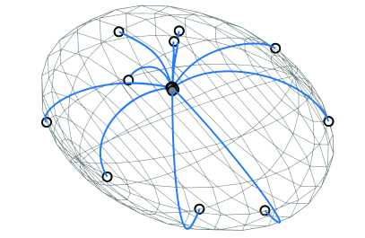
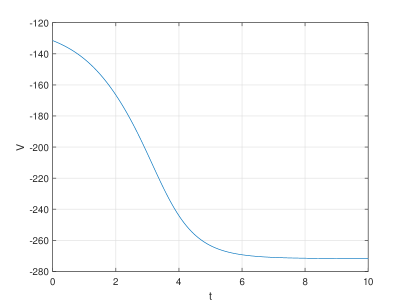
7.1. Illustration of Theorem 3.2

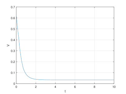
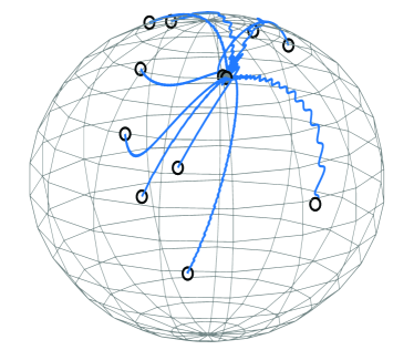
On the left of Figure 1 we can appreciate the motion of 10 tokens on the ellipsoid $(\mathcal{E}_{P}^{2})^{10}$ defined by the randomly generated positive definite symmetric matrix:

$$P=\begin{pmatrix}0.9432&0.0587&-0.1813\\ 0.0587&0.8450&-0.1013\\ -0.1813&-0.1013&0.5519\end{pmatrix},$$

according to the dynamics (8). As expected, all of the tokens converge to a consensus equilibrium. In this case, the dynamics is a gradient vector field and on the right of Figure 1 we show the time evolution of the corresponding potential $V_{P}=V\circ\imath_{P}$ with $V$ defined in (10).

Refer to caption
(a) Convergence to a consensus equilibrium on the ellipsoid $\mathcal{E}^{2}_{P}$.
Refer to caption
(b) Evolution of the potential function $V_{P}=V\circ\imath_{P}$ with $V$ defined in (10).
Figure 1. Illustration of Theorem 3.2.

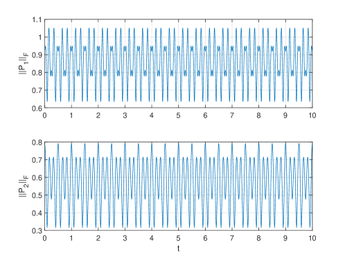
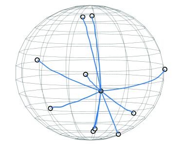
7.2. Illustration of Theorem 4.1

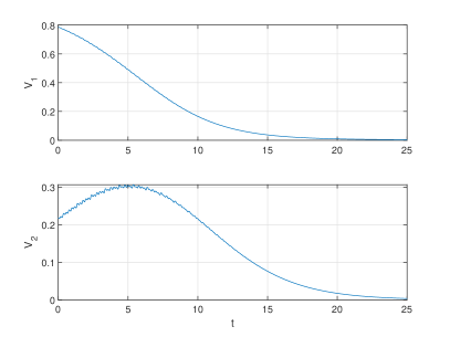
Figure 3 shows the motion of 10 tokens on the sphere $(\mathbb{S}^{2})^{10}$ according to the dynamics (11) with $h=2$. The matrices $P_{1}(t)$ and $P_{2}(t)$ were computed as $P_{1}(t)=D_{1}(t)P_{1}^{\prime}$, $P_{2}(t)=D_{2}(t)P_{2}^{\prime}$ with $P_{1}^{\prime}$ and $P_{2}^{\prime}$ randomly generated:

$$P_{1}^{\prime}=\begin{pmatrix}0.0805&-0.1929&0.1991\\ -0.2312&0.3131&-0.2335\\ 0.1788&-0.1732&-0.1594\end{pmatrix},\quad P_{2}^{\prime}=\begin{pmatrix}-0.3067&0.0349&0.1107\\ 0.0572&-0.0557&0.1343\\ 0.1375&0.1083&0.1018\end{pmatrix},$$

and $D_{1}(t)$ and $D_{2}(t)$ given by:

$$D_{1}=\begin{pmatrix}2\cos(10\pi t)&0&0\\ 0&2\sin(10\pi t)&0\\ 0&0&2\cos(6\pi t)\end{pmatrix},\quad D_{2}=\begin{pmatrix}2\cos(6\pi t)&0&0\\ 0&2\sin(6\pi t)&0\\ 0&0&2\cos(4\pi t)\end{pmatrix}.$$

To better appreciate the time-varying nature of the matrices $P_{1}$ and $P_{2}$, in Figure 2 we shown their Frobenius norm.

Refer to caption
Figure 2. Frobenius norm of the matrices $P_{1}$ and $P_{2}$.
Refer to caption
(a) Convergence to a consensus equilibrium on the sphere $\mathbb{S}^{2}$. All the tokens start and remain in an hemisphere.
Refer to caption
(b) Evolution of the Lyapunov function (13) used in the proof of Theorem 4.1.
Figure 3. Illustration of Theorem 4.1.

On the left of Figure 3 we can appreciate that all the tokens start and remain in an hemisphere and that they converge to a consensus equilibrium. The proof of Theorem 4.1 was based on the Lyapunov function (13) whose time-evolution is displayed on the right of Figure 3 for the case where $v=(1~{}0~{}0)$.

7.3. Illustration of Theorem 6.1

Theorem 6.1 considers the dynamics (21) with $P(t)=D(t)P^{\prime}$, randomly generated $P^{\prime}$ and $U$ given by:

$$P^{\prime}=\begin{pmatrix}0.3598&0.4150&0.1319\\ 0.0971&-0.0668&-0.2046\\ 0.1548&-0.2102&0.1220\end{pmatrix},\quad U=\begin{pmatrix}-0.2590&0.4965&0.5609\\ 0.4965&-0.7174&-0.5003\\ 0.5609&-0.5003&-0.0247\end{pmatrix},$$

and $D(t)$ defined as:

$$D=\begin{pmatrix}2\cos(10\pi t)&0&0\\ 0&2\sin(10\pi t)&0\\ 0&0&2\cos(6\pi t)\end{pmatrix}.$$

On the left of Figure 4 we can observe convergence of the tokens to a consensus equilibrium point whereas on the right we have the time evolution of $V_{1}=1-{\rm y}_{1}^{\top}v$ and $V_{2}=1-{\rm y}_{2}^{\top}v$ where $v\in\mathbb{R}^{3}$ is the eigenvector of $U$ corresponding to its largest eigenvalue. Note that $V_{2}$ is not a Lyapunov function, and therefore it may increase, although the proof of Theorem 6.1, establishes that it will eventually converge to zero.

Refer to caption
(a) Convergence to a consensus equilibrium on the sphere $\mathbb{S}^{2}$. All the tokens start and remain in the hemisphere defined by $v$.
Refer to caption
(b) Evolution of the functions $V_{1}$ and $V_{2}$ used in the proof of Theorem 6.1.
Figure 4. Illustration of Theorem 6.1.

7.4. Illustration of Theorem 5.1
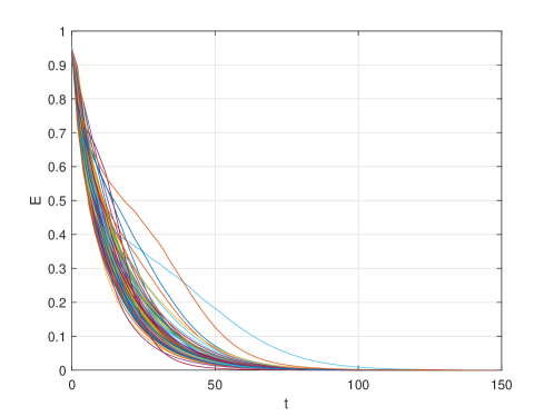
We now consider the dynamics (15) with $50$ tokens each of dimension $500$. The number and dimension of the tokens were chosen to make them comparable to the GPT-2 model. We use two heads ($h=2$) with the matrices $P_{1}=D_{1}(t)P_{1}^{\prime}$ and $P_{2}=D_{2}(t)P_{2}^{\prime}$ obtained by randomly generating $P_{1}^{\prime}$ and $P_{2}^{\prime}$, and taking $D_{1}(t)$ and $D_{2}(t)$ to be diagonal with entries $(D_{\eta})_{jj}=|2\sin(wt+\phi)|$ for $\eta=1,2$, $j=1,\ldots,500$, $w$ drawn from the uniform distribution on $]0,1[$ and $\phi$ drawn from the uniform distribution on $]0,2\pi[$.

In Figure 5 we display the evolution of the function $E:(\mathcal{E}_{W}^{n})^{\ell}\to\mathbb{R}^{+}$ defined as:

(25) $$E=1-\frac{1}{\ell}\sum_{i=0}^{\ell}\frac{|{\rm y}_{1}^{\top}\,{\rm y}_{i}|}{|{\rm y}_{1}|\,|{\rm y}_{i}|},$$

along $100$ trajectories of (15) from random initial conditions drawn from an element-wise uniform distribution on $]-0.5,0.5[$, and then projected to the sphere. The function $E$ only becomes zero when all the tokens are located at the same configuration. We can appreciate in Figure 5 how the function $E$ converges to zero along all the trajectories.

Refer to caption
Figure 5. Illustration of Theorem 5.1; evolution of the function $E$ defined in (25) along $100$ solutions of (15) with random initial conditions drawn from an element-wise uniform distribution on $]-0.5,0.5[$ and then projected to the sphere.

7.5. GPT-2 Experiments

In this section we report on experiments conducted on the GPT-2 Xl model suggesting that our theoretical findings hold under more general assumptions. Since our results are asymptotic, we need to increase the depth of the GPT-2 XL model. We do so by running the same set of tokens through the model multiple times. In other words, we extract the tokens at the end of the model and feed them to the model for another pass thereby simulating a model of increased length. In total, the tokens pass through the model $2000$ times.

In the first experiment, we prompted the model with:

Describe a futuristic city where humans and robots live together.
Talk about what the city looks like and what daily life is like there.

The experiments were conducted on two different configurations of the GPT-2 XL model, the first using the pre-trained weights provided by the Hugging Face library [34], and the second using randomly generated weight matrices. The multiple passes through the model result in matrices $P$ and $U$ that are time-varying but periodic with period corresponding to the depth of the GPT-2 XL model: 48 layers. To measure how far the tokens are from each other we used the function (25) whose evaluation after each pass is depicted in Figure 6.

Refer to caption
Figure 6. Evaluation of the function (25) after each pass through GPT-2 XL with original and random weights.

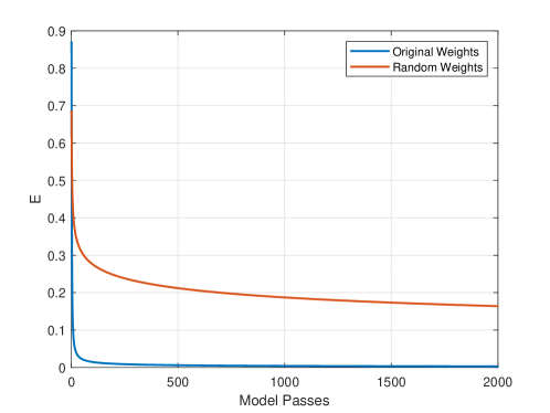
We can observe that for both configurations the function $E$ decreases with each pass through the model thus implying the tokens converge to a consensus equilibrium. We recall that our theoretical results predict this observation only when feedforward layers are absent. These empirical results suggest that token consensus does not depend on the chosen weight matrices. However, this conclusion is predicated on the matrices $P$ and $U$ being periodic.

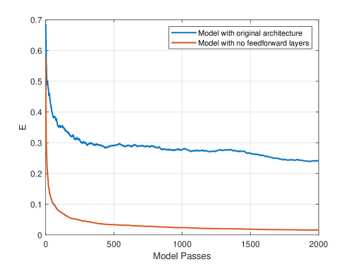
To eliminate the periodicity constraint, we repeated the same experiment while randomly generating all the weight matrices with each pass through the model. In addition, we also performed this test by removing the feedforward layers (including the associated normalization function and skip connection) to better understand the impact of these on token consensus. The results are reported in Figure 7 where we can see that convergence towards consensus still occurs.

Refer to caption
Figure 7. Comparison between original GPT-2 XL architecture and GPT-2 XL with feedforward layers removed; evaluation of the function (25) after each pass through the model; model weights resampled after each model pass.

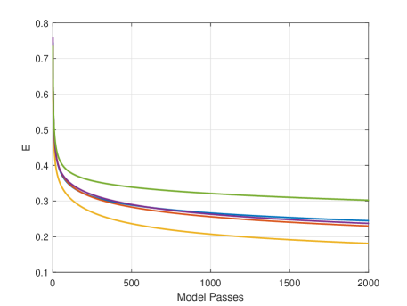
In the next experiment we returned to time-varying periodic matrices $P$ and $U$ randomly picked using a Gaussian distribution with zero mean and standard deviation $0.02$. We randomly picked five sentences from [35], presented in Table 2, to be used as prompts and test if consensus depends on the prompt.

Table 2. Five sentences randomly chosen from [35] to be used as prompts.
Prompts
1. A few colleagues and I amused ourselves at a previous IEEE conference on Decision and Control (CDC) with having ChatGPT try to handle all sorts of things, including a failed attempt at having it find Lyapunov function.
2. The instructions that we gave to ChatGPT were, ’’Write a presidential column for the Control Systems Magazine on the future of control,’’ and the resulting column is given verbatim here:
3. Spearheaded by (CSS) Vice-President for Conference Activities Carolyn Beck and Prof. Philip E. Paré, we arrived at a temporary policy, for now, large-scale language models are not allowed as coauthors.
4. Imagine the absurdity of having to agree that ‘‘By uploading this manuscript, I certify that the computations in this submission are made by hand and no calculator was used to perform any of the computations.’’
5. I have no doubt that our warning message will seem as quaint and obsolete as this statement about calculators within a few years.

Since all the prompts have different lengths each prompt was padded with zeros. The results are present in Figure 8 where it can be seen that all tokens tend to converge to a consensus equilibrium for all the tested inputs.

The final experiment was designed to illustrate the deleterious effects of token consensus, using the prompt:

After endless years lost in the shadows of Shakespeare’s sonnets and the melancholic musings of Pessoa, I have glimpsed enlightenment’s elusive light.
Now, on the precipice of my final hour, as the weight of mortality presses upon me, I must reveal to you the one truth that transcends all others—the meaning of life is...

We performed a series of model passes using the pre-trained GPT-2 XL weights and decoded the output, after $1$, $5$, $10$, $100$, and $1000$ passes, using the classifier layer and a greedy sampling approach333By greedy sampling we mean selecting the output with the highest probability.. The results, presented in Table 3, show that as the number of model passes increases, the generated words become increasingly repetitive illustrating the convergence of the tokens to a consensus equilibrium, i.e., model collapse.

Refer to caption
Figure 8. Evaluation of the function (25) for the five different prompts in [35].
Table 3. Decoded output of the GPT-2 XL model for different number of passes through the model with original model weights.
# passes Decoded phrase
00 (original prompt) After endless years lost in the shadows of Shakespeare’s sonnets and the melancholic musings of Pessoa, I have glimpsed enlightenment’s elusive light. Now, on the precipice of my final hour, as the weight of mortality presses upon me, I must reveal to you the one truth that transcends all others—the meaning of life is…
$1$ the hours of in the m, the’s playsnets, the worksolic poetryings of therouoa, the finally finallyed the. light light. I I I the eveice of a th exams, I I sun of my begins down me, I am face the the the truth thing that Iends all others:the one of life. lovelove
$5$ ,, of, the last, the, time,, the lastol,ing of the,,, I have beened the. last,. I, I the lastit of the last,, I I lasty the, on me, I have have to you my last and I Ien the the.the one of the. to
$10$ ,, of, the last, the,,,, I last,,ing on the S,, I have beening my. last,, I, I the last, of the,,, I I lasty the, on me, I have have to you my last, I,, the,.I last of the. to to
$100$ __ __, in the thermal, the in and_ in in thermal_ in in in thermal __ ___ __ __ ___my in __thermal in_ __the thermal__ the ___in __ __thermal in the in on my, and __ __my the the thermal in in_ in the_ in __thermal_ the_ to __
$1000$ ____/__/_______________________
__/___/_______/_______________/__\__\___

References

  • [1] J. K. Chorowski, D. Bahdanau, D. Serdyuk, K. Cho, and Y. Bengio, “Attention-based models for speech recognition,” Advances in neural information processing systems, vol. 28, 2015.
  • [2] A. Vaswani, N. Shazeer, N. Parmar, J. Uszkoreit, L. Jones, A. N. Gomez, Ł. Kaiser, and I. Polosukhin, “Attention is all you need,” Advances in neural information processing systems, vol. 30, 2017.
  • [3] A. Radford, K. Narasimhan, T. Salimans, I. Sutskever, et al., “Improving language understanding by generative pre-training,” OpenAI, 2018.
  • [4] J. Devlin, M.-W. Chang, K. Lee, and K. Toutanova, “Bert: Pre-training of deep bidirectional transformers for language understanding,” arXiv preprint arXiv:1810.04805, 2018.
  • [5] T. N. Sainath, O. Vinyals, A. Senior, and H. Sak, “Convolutional, long short-term memory, fully connected deep neural networks,” in 2015 IEEE international conference on acoustics, speech and signal processing (ICASSP), pp. 4580–4584, Ieee, 2015.
  • [6] K. O’shea and R. Nash, “An introduction to convolutional neural networks,” arXiv preprint arXiv:1511.08458, 2015.
  • [7] A. Torfi, R. A. Shirvani, Y. Keneshloo, N. Tavaf, and E. A. Fox, “Natural language processing advancements by deep learning: A survey,” arXiv preprint arXiv:2003.01200, 2020.
  • [8] S. Grigorescu, B. Trasnea, T. Cocias, and G. Macesanu, “A survey of deep learning techniques for autonomous driving,” Journal of field robotics, vol. 37, no. 3, pp. 362–386, 2020.
  • [9] B. Van Dijk, T. Kouwenhoven, M. R. Spruit, and M. J. van Duijn, “Large language models: The need for nuance in current debates and a pragmatic perspective on understanding,” arXiv preprint arXiv:2310.19671, 2023.
  • [10] B. Peng, S. Narayanan, and C. Papadimitriou, “On limitations of the transformer architecture,” arXiv preprint arXiv:2402.08164, 2024.
  • [11] Y. Dong, J.-B. Cordonnier, and A. Loukas, “Attention is not all you need: Pure attention loses rank doubly exponentially with depth,” in International Conference on Machine Learning, pp. 2793–2803, PMLR, 2021.
  • [12] R. Feng, K. Zheng, Y. Huang, D. Zhao, M. Jordan, and Z.-J. Zha, “Rank diminishing in deep neural networks,” Advances in Neural Information Processing Systems, vol. 35, pp. 33054–33065, 2022.
  • [13] B. Geshkovski, C. Letrouit, Y. Polyanskiy, and P. Rigollet, “The emergence of clusters in self-attention dynamics,” arXiv preprint arXiv:2305.05465, 2023.
  • [14] B. Geshkovski, H. Koubbi, Y. Polyanskiy, and P. Rigollet, “Dynamic metastability in the self-attention model,” arXiv preprint arXiv:2410.06833, 2024.
  • [15] B. Geshkovski, C. Letrouit, Y. Polyanskiy, and P. Rigollet, “A mathematical perspective on transformers,” arXiv preprint arXiv:2312.10794, 2023.
  • [16] Y. Lu, Z. Li, D. He, Z. Sun, B. Dong, T. Qin, L. Wang, and T.-Y. Liu, “Understanding and improving transformer from a multi-particle dynamic system point of view,” arXiv preprint arXiv:1906.02762, 2019.
  • [17] S. Dutta, T. Gautam, S. Chakrabarti, and T. Chakraborty, “Redesigning the transformer architecture with insights from multi-particle dynamical systems,” arXiv preprint arXiv:2109.15142, 2021.
  • [18] A. Sarlette and R. Sepulchre, “Consensus optimization on manifolds,” SIAM journal on Control and Optimization, vol. 48, no. 1, pp. 56–76, 2009.
  • [19] J. Markdahl, J. Thunberg, and J. Gonçalves, “Almost global consensus on the $n$-sphere,” IEEE Transactions on Automatic Control, vol. 63, no. 6, pp. 1664–1675, 2017.
  • [20] J. Thunberg, J. Markdahl, F. Bernard, and J. Goncalves, “A lifting method for analyzing distributed synchronization on the unit sphere,” Automatica, vol. 96, pp. 253–258, 2018.
  • [21] E. Sontag, “Smooth stabilization implies coprime factorization,” IEEE Transactions on Automatic Control, vol. 34, no. 4, pp. 435–443, 1989.
  • [22] E. D. Sontag, “The ISS philosophy as a unifying framework for stability-like behavior,” in Nonlinear control in the year 2000 volume 2 (A. Isidori, F. Lamnabhi-Lagarrigue, and W. Respondek, eds.), (London), pp. 443–467, Springer London, 2001.
  • [23] E. D. Sontag, Input to State Stability: Basic Concepts and Results, pp. 163–220. Berlin, Heidelberg: Springer Berlin Heidelberg, 2008.
  • [24] W. Ren, R. Beard, and E. Atkins, “A survey of consensus problems in multi-agent coordination,” in Proceedings of the 2005, American Control Conference, 2005., pp. 1859–1864 vol. 3, 2005.
  • [25] Y. Cao, W. Yu, W. Ren, and G. Chen, “An overview of recent progress in the study of distributed multi-agent coordination,” IEEE Transactions on Industrial Informatics, vol. 9, no. 1, pp. 427–438, 2013.
  • [26] R. E. Turner, “An introduction to transformers,” 2024. https://arxiv.org/abs/2304.10557.
  • [27] N. Karagodin, Y. Polyanskiy, and P. Rigollet, “Clustering in causal attention masking,” arXiv preprint arXiv:2411.04990, 2024.
  • [28] J. L. Ba, J. R. Kiros, and G. E. Hinton, “Layer normalization,” arXiv preprint arXiv:1607.06450, 2016.
  • [29] A. Q. Jiang, A. Sablayrolles, A. Mensch, C. Bamford, D. S. Chaplot, D. d. l. Casas, F. Bressand, G. Lengyel, G. Lample, L. Saulnier, et al., “Mistral 7b,” arXiv preprint arXiv:2310.06825, 2023.
  • [30] Z. Lin, B. Francis, and M. Maggiore, “State agreement for continuous-time coupled nonlinear systems,” SIAM J. Control and Optimization, vol. 46, pp. 288–307, 01 2007.
  • [31] H. Khalil, “Nonlinear systems,” 3rd edition, 2002.
  • [32] J. G. Wendel, “A problem in geometric probability,” Mathematica Scandinavica, vol. 11, no. 1, pp. 109–111, 1962.
  • [33] H. Khalil, Nonlinear Systems. Prentice Hall, 3rd ed., 2002.
  • [34] T. Wolf, L. Debut, V. Sanh, J. Chaumond, C. Delangue, A. Moi, P. Cistac, T. Rault, R. Louf, M. Funtowicz, et al., “Transformers: State-of-the-art natural language processing,” in Proceedings of the 2020 conference on empirical methods in natural language processing: system demonstrations, pp. 38–45, 2020.
  • [35] M. Egerstedt, “Chatbots as tools or existential threats [president’s message],” IEEE Control Systems Magazine, vol. 44, no. 1, pp. 7–8, 2024.