Perspective: Time irreversibility in systems observed at coarse resolution

Abstract

A broken time-reversal symmetry, i.e. broken detailed balance, is central to non-equilibrium physics and is a prerequisite for life. However, it turns out to be quite challenging to unambiguously define and quantify time-reversal symmetry (and violations thereof) in practice, that is, from observations. Measurements on complex systems have a finite resolution and generally probe low-dimensional projections of the underlying dynamics, which are well known to introduce memory. In situations where many microscopic states become “lumped” onto the same observable “state” or when introducing “reaction coordinates” to reduce the dimensionality of data, signatures of a broken time-reversal symmetry in the microscopic dynamics become distorted or masked. In this perspective we highlight why in defining and discussing time-reversal symmetry, and quantifying its violations, the precise underlying assumptions on the microscopic dynamics, the coarse graining, and further reductions, are not a technical detail. These assumptions decide whether the conclusions that are drawn are physically sound or inconsistent. We summarize recent findings in the field and reflect upon key challenges.

I Introduction

A broken time-reversal symmetry, or broken detailed balance, is essential for the existence of living matter [1, 2, 3]. Stated from a thermodynamic perspective, the emergence and persistence of life requires constant entropy production [4, 3]. These two statements are intuitive and may nowadays seem obvious, perhaps rightfully so. However, an attempt to unambiguously define time-reversal symmetry (and violations thereof) and consistently connect it to thermodynamics purely in terms of observations turns out to be rather non-trivial. Avoiding the conceptually much harder problem of the emergence of a positive entropy production from mechanics (classical or quantum) [5, 6], the main difficultly we are referring to in this perspective is to define, understand, and infer violations of detailed balance in a system’s dynamics when one cannot observe all degrees of freedom. There may be cases, where one at least has some knowledge about how the observable depends on the relevant (i.e., “slow”; to be made precise later), hidden microscopic degrees of freedom, and in some cases one does not even have such knowledge.

From a practical perspective, measurements on complex systems either have a finite resolution [7, 8, 9, 10] or do not resolve all relevant degrees of freedom—they only probe low-dimensional projections of the dynamics, such as the magnetization [11] or dielectric response [12], and observables such as molecular extensions or FRET efficiencies and lifetimes in single-molecule experiments [13, 14, 15, 16, 17, 18, 19, 20]. It is well known that these projections typically introduce memory [21, 22, 23]. In these situations, many microscopic states become “lumped” onto the same observable “state”. Similar projections emerge when introducing “reaction coordinates” to reduce the dimensionality of data to the essential observable(s) [24, 25, 26], which is taken a step further if one constructs kinetic (typically Markov) models with a small number of most relevant, long-lived states [27, 28, 29]. These projections and reductions significantly distort or mask signatures of a broken time-reversal symmetry in microscopic dynamics. The main aim of this perspective is not on biological applications [30], but to highlight why in defining and discussing time-reversal symmetry, and quantifying its violations, the precise underlying assumptions on the microscopic dynamics, the projection/coarse graining, and further reductions, are not merely a technical detail. These assumptions typically decide whether the conclusions that are drawn are physically correct or inconsistent, and in turn whether they lead to controversy.

Defining the entropy production rate based on some general observable (i.e., without knowledge about microscopic dynamics) from first principles is non-trivial. While irreversibility implies that microscopic trajectories evolving “forwards” in time are not equally likely as their time-reversed counterparts, the situation is typically very different when we observe only projections and/or discretized trajectories. To motivate this claim, we note the “oddness” of certain degrees of freedom (like momenta) under time-reversal. Note that the sign-change is a post factum rule, there is no necessary mathematical condition for assuming it, it is enforced to align with observations.

Inertia is essentially nothing but the persistence of motion, and memory effects may, consistently, be considered a generalization of this (trivial) persistence. In other words, memory effects are, strictly speaking, manifested as (anti-)persistence of motion—a particle is more (or less) likely to move in the instantaneous direction or to transition into another state depending on the past. It should not be difficult to appreciate that deciding about a possible “sign change” of general memory effects is far from trivial. In other words, in general (except if assuming that everything that is hidden is at equilibrium [31]) one cannot simply “flip the sign” of memory effects.

This perspective is written to highlight, by examples, possible inconsistencies of, and incompatibilities between, common underlying assumptions. For the sake of simplicity we will focus on situations where the “microscopic” dynamics is an overdamped Markovian dynamics. To ease the reading, we refrain from being rigorous, but we nevertheless insist on being consistent and, as far as feasible, precise. We will express entropy in units of Boltzmann’s constant $k_{\rm B}$ and energy in units of thermal energy $k_{\rm B}T$ at temperature $T$.

II Entropy production in Markovian systems coupled to an equilibrium bath

A meaningful definition of entropy production ought to measure the discrepancy between the probability of forward paths, $(x_{\tau})_{0\leq\tau\leq t}$, $\mathbbm{P}[(x_{\tau})_{0\leq\tau\leq t}]$, and the probability of time-reversed paths, $(\theta x_{\tau})_{0\leq\tau\leq t}$, $\widetilde{\mathbbm{P}}[(\theta x_{\tau})_{0\leq\tau\leq t}]$, where the backwards paths may be measured with a different probability measure $\widetilde{\mathbbm{P}}$ than the forwards paths, and hence may refer to a different ensemble [32]. A priori there are many possibilities to quantify a discrepancy, e.g., any $L^{p}$ norm. However, the definition for Markovian dynamics that turns out to be consistent with classical (phenomenological) thermodynamics is the Kullback-Leibler divergence [33, 32],

$$S_{\rm inf} =\int\mathrm{d}\mathbbm{P}[(x_{\tau})_{0\leq\tau\leq t}]\ln\frac{\mathbbm{P}[(x_{\tau})_{0\leq\tau\leq t}]}{\widetilde{\mathbbm{P}}[(\theta x_{\tau})_{0\leq\tau\leq t}]}.$$ (1)

$S_{\rm inf}\equiv S_{\rm inf}[0,t]$ is called the informatic entropy production in the interval $[0,t]$ [32], as it a priori does not necessarily relate to the thermodynamic entropy production. One may also write $S_{\rm inf}=\langle\Delta s_{\rm inf}[(x_{\tau})_{0\leq\tau\leq t}]\rangle$ which is the expectation $\langle\cdots\rangle$ of the stochastic path-wise entropy production $\Delta s_{\rm inf}[(x_{\tau})_{0\leq\tau\leq t}]\equiv\ln(\mathbbm{P}[(x_{\tau})_{0\leq\tau\leq t}]/\widetilde{\mathbbm{P}}[(\theta x_{\tau})_{0\leq\tau\leq t}])$ [34] in the forward path ensemble $\mathbbm{P}[(x_{\tau})_{0\leq\tau\leq t}]$. Only for a physically consistent choice of time reversal $\theta$ and backwards measure $\widetilde{\mathbbm{P}}$ they may become equivalent, which will be discussed in more detail below.

From $\frac{\widetilde{\mathbbm{P}}[(\theta x_{\tau})_{0\leq\tau\leq t}]}{\mathbbm{P}[(x_{\tau})_{0\leq\tau\leq t}]}={\rm e}^{-\Delta s_{\rm inf}[(x_{\tau})_{0\leq\tau\leq t}]}$ and

$$1 =\int{\rm d}\mathbbm{P}[(x_{\tau})_{0\leq\tau\leq t}]=\int\mathrm{d}\mathbbm{P}[(x_{\tau})_{0\leq\tau\leq t}]\frac{\widetilde{\mathbbm{P}}[(\theta x_{\tau})_{0\leq\tau\leq t}]}{\mathbbm{P}[(x_{\tau})_{0\leq\tau\leq t}]}$$

$$=\left\langle{\rm e}^{-\Delta s_{\rm inf}[(x_{\tau})_{0\leq\tau\leq t}]}\right\rangle\geq{\rm e}^{-\Delta S_{\rm inf}},$$

where in the last step we used Jensen’s inequality for the convex exponential function and Eq. (1), follows the detailed fluctuation theorem $\langle{\rm e}^{-\Delta s_{\rm inf}}\rangle=1$ and non-negativity of the entropy production (i.e., the second law) $\Delta S_{\rm inf}\geq 0$.

For brevity and sake of simplicity we will limit the subsequent discussion to situations, where the detailed, “microscopic” dynamics corresponds to an overdamped diffusion (with additive noise) in $d$ dimensions and obeys local detailed balance[33, 35, 36]. Then, the relevant (“slow”) degrees of freedom $x_{t}\in\mathbbm{R}^{d}$ obey the Itô equation with symmetric positive-definite $d\times d$ diffusion matrix $D$ proportional to the temperature, $D\propto T$ reflecting the effect of a heat bath containing all irrelevant (“fast”) degrees of freedom (at all times) at equilibrium at temperature $T$, and a drift $a(x):\mathbbm{R}^{d}\to\mathbbm{R}^{d}$ for simplicity without explicit time dependence [37],

$$\mathrm{d}x_{\tau}=a(x_{\tau})\mathrm{d}\tau+\sqrt{2D}\mathrm{d}W_{\tau},$$ (2)

with $\langle\mathrm{d}W^{i}_{\tau}\rangle=0$ and $\langle\mathrm{d}W^{i}_{\tau}\mathrm{d}W^{j}_{\tau^{\prime}}\rangle=\delta_{ij}\delta(\tau-\tau^{\prime})\mathrm{d}\tau\mathrm{d}\tau^{\prime}$. The probability density of $x_{\tau}$, $p(x,\tau)$, obeys the Fokker-Planck equation [38], which is a continuity equation $\partial_{t}p(x,\tau)=-\nabla\cdot j(x,\tau)$ with probability current $j(x,\tau)\equiv\nu(x,\tau)p(x,\tau)$ that depends on the local mean velocity $\nu(x,\tau):\mathbbm{R}^{d}\times[0,\infty)\to\mathbbm{R}^{d}$, defined as

$$\nu(x,\tau) \equiv\frac{\left[a(x)-D\nabla\right]p(x,\tau)}{p(x,\tau)}.$$ (3)

II.1 Thermodynamic entropy production

While path-wise, stochastic definitions of the entropy production exist [34], throughout this perspective we focus on the deterministic, average values. We first address steady-state dynamics with invariant density $p_{\rm s}(x)$, i.e., we first consider strongly ergodic systems relaxing to an invariant density $p(x,\tau\to\infty)=p_{\rm s}(x)$, which requires $a(x)$ to be sufficiently confining. We either prepare the system in the steady state, i.e., $x_{\tau=0}\sim p_{\rm s}(x)$, or begin our observations after a sufficiently long time. Such systems may be in thermodynamic equilibrium (these are referred to as being in “detailed balance”), where no entropy is produced. Conversely, a system in the stationary state may also perform work $W$ against the friction [33]

$$W =\left\langle\int_{0}^{t}[D^{-1}a(x_{\tau})]\cdot\circ\mathrm{d}x_{\tau}\right\rangle_{\rm s}$$

$$=t\left\langle\nu_{\rm s}^{T}(x)D^{-1}\nu_{\rm s}(x)\right\rangle_{\rm s}\geq 0,$$ (4)

where $\left\langle\cdots\right\rangle_{\rm s}$ denotes the steady-state ensemble average, $\circ$ the stochastic Stratonovich integral, and we introduced the invariant local mean velocity $\nu_{\rm s}(x)=\nu(x,\tau\to\infty)$. The non-negativity of $W$ follows from the fact that $D$ is positive definite. Steady-state systems with $W>0$ are said to be out of equilibrium or dissipative. The system is connected to a heat bath with temperature $T$, such that the work $W$ gives rise to an entropy production in the medium $\Delta S_{\rm med}=W/T$, where the $\Delta$ notation always refers to entropy produced in the time interval $[0,t]$, i.e., $\Delta S\equiv S(t)-S(0)$. In steady states under the assumptions on the heat bath mentioned above, this is the only source of entropy production, such that the total thermodynamic entropy production is given by [33]

$$\Delta S_{\rm tot}=\Delta S_{\rm med}\geq 0\,.$$ (5)

For any non-stationary preparation of the system, $p(x,\tau=0)\neq p_{\rm s}(x)$, the probability density changes in time and there is an additional contribution to entropy production, namely the change of Gibbs-Shannon entropy in the system [33]

$$\Delta S_{\rm sys}=-\int\mathrm{d}x\,p(x,t)\ln p(x,t)+\int\mathrm{d}x\,p(x,0)\ln p(x,0)\,,$$ (6)

which can also take on negative values. Similarly, $\Delta S_{\rm med}$ (and thus $W$) can be positive or negative for non-steady-state dynamics. During transients the total thermodynamic entropy production reads [34, 33],

$$\Delta S_{\rm tot} =\Delta S_{\rm med}+\Delta S_{\rm sys}$$

$$=\int_{0}^{t}\mathrm{d}\tau\langle\nu^{T}(x,\tau)D^{-1}\nu(x,\tau)\rangle\geq 0\,,$$ (7)

where $\langle\cdot\rangle$ denotes the expectation over $p(x,\tau)$. At thermodynamic equilibrium $\Delta S_{\rm tot}=0$.

Although $\Delta S_{\rm sys}$ and $\Delta S_{\rm med}$ can be positive, negative, or zero, we note that it is not possible to have $\Delta S_{\rm sys}=-\Delta S_{\rm med}\neq 0$. That is, we cannot have $\Delta S_{\rm tot}=0$ when $\Delta S_{\rm sys}\neq 0$ or $\Delta S_{\rm med}\neq 0$. To see this, note that $\Delta S_{\rm sys}\neq 0$ implies that $\partial_{\tau}p(x,\tau)\neq 0$, which via the Fokker-Planck equation (3) gives $\nu(x,\tau)\neq 0$ for some $x,\tau$, in turn implying $\Delta S_{\rm tot}\neq 0$ via Eq. (7). The fact that any evolution of $p(x,\tau)$ bounds $\Delta S_{\rm tot}$ from below by a positive constant is formally encoded in the Benamou-Brenier formula [39, 40] and further in thermodynamic bounds on transport [41].

II.2 Equivalence of thermodynamic and informatic entropy production for overdamped Markov dynamics

Whereas the Onsager-Machlup formula for the “stochastic action” entering path probabilities [42] in Eq. (1) are well known in the physics literature, their meaning is far from trivial. Namely, the action of a path $(x_{\tau})_{0\leq\tau\leq t}$ governed by Eq. (2) is assumed to read

$$A[(x_{\tau})_{0\leq\tau\leq t}]$$ (8)

$$=\frac{1}{4}\int_{0}^{t}\mathrm{d}\tau\{[\dot{x}_{\tau}-a(x_{\tau})]^{T}D^{-1}[\dot{x}_{\tau}-a(x_{\tau})]+2\nabla\cdot a(x_{\tau})\},$$

where $\dot{x}_{\tau}\equiv\frac{\mathrm{d}x_{\tau}}{\rm d\tau}$ and note that the last term does not appear in the small-noise limit [43] but is neccessary in general (see Theorem 9.1 and Corollary in Chapter VI of Ref. [44]). Notably, it is well known that $\mathbbm{P}(|\dot{x}_{\tau}|<C)=0$ for any $C<\infty$ and any $\tau$, so Eq. (8) should cause (substantial) concern, since paths are locally almost surely non-differentiable. The issue may be resolved by recalling the support theorem of diffusion [45], according to which (loosely speaking) the probability measure of nowhere differentiable diffusion paths $(x_{\tau})_{0\leq\tau\leq t}$ has support on the closure of smooth paths $(y(\tau))_{0\leq\tau\leq t}\in C^{\infty}$, as long as said smooth approximations are interpreted according to the Stratonovich convention. The Stratonovich formulation is required for consistency between systems with “smooth” and “Brownian” inputs (see also [46]). In this context, we ought to make the replacement $x_{\tau}\to y(t)$ in Eq. (8) along the following lines.

The rigorous probabilistic definition of the Onsager-Machlup functional (see Theorem 9.1 and Corollary in Chapter VI of Ref. [44]) follows from a comparison of probabilities of $x_{\tau}$ remaining within a “tube” of radius $\varepsilon$ around a smooth path $y(t)\in C^{\infty}$ relative to the probability that the Wiener process remains within a straight “tube” of radius $\varepsilon$. To state this precisely we note that

$${\mathbbm{P}}[(x_{\tau})_{0\leq\tau\leq t}] =\mathbbm{P}[(x_{\tau})_{0\leq\tau\leq t}|x_{0}]p(x_{0},0)$$

$$\widetilde{\mathbbm{P}}[(\theta x_{\tau})_{0\leq\tau\leq t}] =\mathbbm{P}[(\theta x_{\tau})_{0\leq\tau\leq t}|x_{t}]p(x_{t},t),$$ (9)

and as well as the supremum norm

$$\|y(\tau)-x_{\tau}\|_{0\leq\tau\leq t}\equiv\sup_{0\leq\tau\leq t}\sup_{i=1,\dots,d}|y_{i}(\tau)-x_{i}(\tau)|,$$ (10)

such that

$$\lim_{\varepsilon\to 0}\frac{\mathbbm{P}\left[\|y(\tau)-x_{\tau}\|_{0\leq\tau\leq t}<\varepsilon\right]}{\mathbbm{P}[\|\sqrt{2D}W_{\tau}\|_{0\leq\tau\leq t}<\varepsilon]}=\mathrm{e}^{-A[(y(\tau))_{0\leq\tau\leq t}]}p(y(0),0),$$ (11)

where $p(y(0))$ is the probability density of the initial condition and we used Eq. (9). The same holds true for the time-reversed path, which for overdamped Markov processes is simply $(\theta x_{\tau})_{0\leq\tau\leq t}=(x_{t-\tau})_{0\leq\tau\leq t}$, which using Eq. (9) reads [32]

$$\lim_{\varepsilon\to 0} \frac{\mathbbm{P}\left[\|y(t-\tau)-x_{t-\tau}\|_{0\leq\tau\leq t}<\varepsilon\right]}{\mathbbm{P}[\|\sqrt{2D}W_{\tau}\|_{0\leq\tau\leq t}<\varepsilon]}$$

$$=\mathrm{e}^{-A^{\dagger}[(y(\tau))_{0\leq\tau\leq t}]}p(y(t),t),$$ (12)

where we introduced the “backward action”

$$A^{\dagger}[(y(\tau) )_{0\leq\tau\leq t}]=\frac{1}{4}\int_{0}^{t}\mathrm{d}\tau\{[\dot{y}(\tau)+a(y(\tau))]^{T}\times$$

$$D^{-1}[\dot{y}(\tau)+a(y(\tau))]+2\nabla\cdot a(y(\tau))\}.$$ (13)

Note that thermodynamic consistency requires that the probability measures of forward and backwards paths are equivalent, i.e., $\mathbbm{P}[(x_{\tau})_{0\leq\tau\leq t}]>0\iff\widetilde{\mathbbm{P}}[(\theta x_{\tau})_{0\leq\tau\leq t}]>0$ [33]. The fraction in Eq. (1) is non-zero on the support of $\mathbbm{P}[(x_{\tau})_{0\leq\tau\leq t}]$. As a result we have on the support of $\mathbbm{P}[(x_{\tau})_{0\leq\tau\leq T}]$

$$\frac{\mathbbm{P}[(y(\tau))_{0\leq\tau\leq t}]}{\mathbbm{P}[(y(t-\tau))_{0\leq\tau\leq t}]} =\frac{\lim_{\varepsilon\to 0}\frac{\mathbbm{P}\left[\|y(\tau)-x_{\tau}\|_{0\leq\tau\leq t}<\varepsilon\right]}{\mathbbm{P}[\|\sqrt{2D}W_{\tau}\|_{0\leq\tau\leq t}<\varepsilon]}}{\lim_{\varepsilon\to 0}\frac{\mathbbm{P}\left[\|y(t-\tau)-x_{t-\tau}\|_{0\leq\tau\leq t}<\varepsilon\right]}{\mathbbm{P}[\|\sqrt{2D}W_{\tau}\|_{0\leq\tau\leq t}<\varepsilon]}}$$

$$=\mathrm{e}^{-A+A^{\dagger}}\frac{p(y(0),0)}{p(y(t),t)}.$$ (14)

and in turn, since $-A+A^{\dagger}=\int_{0}^{t}a(y(\tau))^{T}D^{-1}\dot{y}(\tau)\mathrm{d}\tau=\int_{0}^{t}[D^{-1}a(y(\tau))]\cdot\dot{y}(\tau)\mathrm{d}\tau$, we have on the support of $\mathbbm{P}[(x_{\tau})_{0\leq\tau\leq t}]$

$$\Delta s_{\rm inf}[(x_{\tau})_{0\leq\tau\leq t}]=\int_{\tau=0}^{\tau=t}[D^{-1}a(x_{\tau})]\cdot\circ\mathrm{d}x_{\tau}+\ln\frac{p(x_{0},0)}{p(x_{t},t)}.$$ (15)

For steady-state dynamics we have $p(x,0)=p(x,t)=p_{\rm s}(x)$ such that the logarithmic term vanishes, and upon taking the average and using Eq. (3) we recover $\Delta S_{\rm inf}=W/T$ with $W$ given in Eq. (4). More generally, for any initial condition $p(x_{0},0)$ we obtain Eq. (7). For overdamped diffusions the informatic and thermodynamic entropy production are hence equivalent, $\Delta S_{\rm tot}=\Delta S_{\rm inf}$. Note that these results follow more directly from the Radon-Nikodym theorem [47].

Another deep path-wise result we want to mention here is known as Watanabe’s formula (see Refs. [47, 48] and Theorem 9.2 in Ref. [44]) which states for overdamped diffusion that any smooth closed curve $\Gamma\in C^{\infty}$, i.e., $\bar{y}(\tau)\in C^{\infty}$ in $\mathbbm{R}^{d}$ such that $\bar{y}(0)=\bar{y}(t)$, we have

$$\frac{\mathbbm{P}[(\bar{y}(\tau))_{0\leq\tau\leq t}|y(0)]}{\mathbbm{P}[(\bar{y}(t-\tau))_{0\leq\tau\leq t}|y(t)]} =\exp\left(\int_{0}^{t}a(\bar{y}(\tau))^{T}D^{-1}\dot{\bar{y}}(\tau)\mathrm{d}\tau\right)$$

$$=\exp\left(\oint_{\Gamma}[D^{-1}a(\bar{y})]\cdot\mathrm{d}\bar{y}\right),$$ (16)

where $\oint_{\Gamma}D^{-1}a\cdot\mathrm{d}\bar{y}$ is known as the “cycle force” [49]. The fraction equals 1 if and only if $x_{t}$ obeys detailed balance, $D^{-1}a=-\nabla\phi$ (i.e., when $D^{-1}a(x)$ is an exact one-form).

III Dynamics at coarse resolution

III.1 Markovian coarse-grained dynamics

When the (generalized) potential $\phi(x)\equiv-\ln p_{\rm s}(x)$ features deep wells separated by high (and sharp) barriers [50] and under some additional (but commonly met) requirements on the irreversible component of $a(x)$, $a(x)-D\nabla\phi(x)$ [51], the time-scales of so-called “librational” motions inside the wells and transitions between the wells are sufficiently separated. Moreover, if (and only if [50, 52, 53, 54]) the dynamics are projected onto sufficiently localized cores centered at the minima [50] (also referred to as “milestones” [55, 52, 53]), (see Fig. 1 as well as the Kramers-type result in Fig. 2), the resulting slow, long-time-scale “hopping” dynamics between the cores is a Markov process. That is, time-scale separation ensured by the nominal features of $a(x)$ is by itself not sufficient for the emerging process to be Markov, a particular type of coarse graining, nowadays commonly referred to as “milestoning” [56, 55, 53, 52, 57] is required as well. The reason why naively “cutting” the configuration space into pieces—a process referred to as “lumping”—cannot give rise to Markov dynamics on the discrete state space is that by lumping we (i) inherently (and inevitably) include the fast librational motions and rapid re-crossings of the barriers (see Figs. 1c and 2c) and (ii) the transition probabilities and waiting times in the coarse-grained states depend on previous states [50, 52, 54]. Note that issues (i) and (ii) equally emerge when a many-state discrete-state jump process is lumped to fewer states.

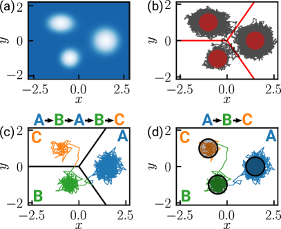
Figure 1: (a) A free-energy landscape $\phi(\mathbf{x})$ (white to blue) with three minima. (b) Overdamped motion $\mathrm{d}\mathbf{x}_{\tau}=-D\nabla\phi(\mathbf{x}_{\tau})+\sqrt{2D}\mathrm{d}\mathbf{W}_{\tau}$ (grey) can be coarse grained into three states using lumping (e.g., see three areas separated by lines) or using three milestones (e.g., see circles). Only the latter procedure will approach Markovian dynamics for deep and well separated minima. (c) Lumping and (d) milestoning sketched for part of the trajectory with a reduced time resolution.

Recall that as soon as the waiting time in the discrete states is not exponentially distributed or depends on previous states, the coarse-grained jump process is not Markovian. To make this explicit, only milestoning-type of coarse grainings may yield Markov jump dynamics in the presence of a time-scale separation, whereas lumping does not [55, 52, 53]. Beside not calling it “milestoning”, this fact was realized already by Kramers in his seminal work [58] (see Figure 2 and note that Kramers’ partitioning of configuration space is a prime example of milestoning; for more details see Supplemental Material in Ref. [54]). It is also very well established in the community building Markov-state models [55, 53]. Yet, it has only recently becoming appreciated in Stochastic Thermodynamics [52, 54, 57, 59, 60, 61] which we will address below in more detail.

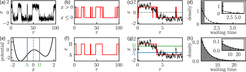
Figure 2: Numerical evaluation of one-dimensional barrier crossing. (a, e) Dynamics $\mathrm{d}x_{\tau}=-\partial_{x}\phi(x)\mathrm{d}\tau+\sqrt{2}\mathrm{d}W_{\tau}$ evolving in a double-well potential $\phi(x)=x^{4}-3x^{2}+x/2$ simulated with $\mathrm{d}\tau=0.01$. The sample trajectory (a) is coarse-grained into two states by lumping $x\leq 0$ and $x>0$ (b) or milestoning with $A=-0.6$ and $B=0.6$ (f), where in the latter procedure the coarse-grained state changes once the milestones $A$ or $B$ are reached. Zoom into the initial part of the trajectory highlights frequent state changes (“fast re-crossings”) in the lumped dynamics (c) compared to (g) the milestoned dynamics. Waiting time density for state changes inferred as a histogram from a very long trajectory ($5\times 10^{7}$ time steps) for (d) lumped for the transition $x>0\to x\leq 0$ (Inset: for the transition $x\leq 0\to x>0$) and (h) milestoned for the transition $B\to A$ (Inset: for the transition $A\to B$) dynamics reveal that only the latter agrees with the desired exponential (black dashed line is $\lambda\exp(-\lambda t)$ for $\lambda^{-1}=$ mean waiting time). Note that the lumped trajectories (b, c) and waiting times (d) explicitly depend on the time resolution and do not converge as $\mathrm{d}\tau\to 0$.

Assuming the coarse-grained dynamics (to a sufficient approximation) corresponds to a Markov process (i.e., implicitly assuming that it emerged from a milestoning-type of coarse-graining, see Fig. 1d), a trajectory $(x_{\tau})_{0\leq\tau\leq t}$ corresponds to a sequence of digitized, say $N$, states. The evolution of the probability of said states encoded in the probability vector $p(t)\in(\mathbbm{R}^{+})^{N}$ follows a master equation [62, 37] $\frac{\mathrm{d}}{\mathrm{d}t}p(t)=Lp(t)$ where $L$ is an $N\times N$ matrix whose elements $L_{ij}=r_{ji}$ for $i\neq j$ are transition rates between states $j\to i$ and $L_{ii}=-\sum_{j\neq i}L_{ji}$. We remind ourselves that the Markov-jump process is an approximation to the long-time-scale dynamics of the microscopic system only, i.e., temporal resolution is lost. Therefore, Markov-jump models correspond to a less general class of dynamics and are in fact already captured (including short-time motions) in diffusion models, a fact that is occasionally forgotten.

Analogously to overdamped diffusion in Eq. (4), a system in a non-equilibrium stationary state with state probability vector $p_{\rm s}$ may perform work, which in the Markov-jump case reads [33] $W=\frac{1}{2}\sum_{i,j}[(p_{\rm s})_{j}r_{ji}-(p_{\rm s})_{i}r_{ij}]\ln({r_{ji}}/{r_{ij}})$, giving rise to an entropy production in the medium $\Delta S_{\rm med}=W/T$. In steady states, this is the only source of entropy production, such that $\Delta S_{\rm tot}=\Delta S_{\rm med}\geq 0$. For any non-stationary preparation of the system, $p(0)\neq p_{\rm s}$, the probability density changes in time and there is an additional contribution to entropy production—the change of Gibbs-Shannon entropy in the system [62, 33, 63],

$$\Delta S_{\rm tot}= \int_{0}^{t}\mathrm{d}\tau\bigg{[}\frac{1}{2}\sum_{i,j}[p_{j}(\tau)r_{ji}-p_{i}(\tau)r_{ij}]\ln\frac{r_{ji}}{r_{ij}}$$

$$+\frac{1}{2}\sum_{i,j}[p_{j}(\tau)r_{ji}-p_{i}(\tau)r_{ij}]\ln\frac{p_{j}(\tau)}{p_{i}(\tau)}\bigg{]}$$ (17)

$$= \frac{1}{2}\int_{0}^{t}\mathrm{d}\tau\sum_{i,j}[p_{j}(\tau)r_{ji}-p_{i}(\tau)r_{ij}]\ln\frac{p_{j}(\tau)r_{ji}}{p_{i}(\tau)r_{ij}}\geq 0\,,$$

where non-negativity follows immediately from the fact that $p_{j}(\tau)r_{ji}-p_{i}(\tau)r_{ij}$ and $\ln[{p_{j}(\tau)r_{ji}}/{p_{i}(\tau)r_{ij}}]$ always have the same sign. Similar to Sec. II.2, also for Markov-jump processes the correct time reversal that yields $\Delta S_{\rm tot}=\Delta S_{\rm inf}$ is $(\theta x_{\tau})_{0\leq\tau\leq t}=(x_{t-\tau})_{0\leq\tau\leq t}$ [33, 32]. Essential for thermodynamic consistency of Markov-jump processes is the so-called local detailed balance [33, 35, 36, 52, 54], which in this particular case corresponds to

$$\ln\frac{r_{ij}}{r_{ji}}=\Delta S_{i\to j},$$ (18)

stating that the log-ratio of forward and backward transition rates corresponds to the entropy flow along the transition. We note that time-scale separation is certainly necessary but not sufficient for local detailed balance to emerge; a coarse-grained dynamics that is accurately represented by a Markov-jump process obeying local detailed balance should, as a rule, be understood as not emerging from lumping, but instead from a reduction like milestoning [52, 54].

We remark that the second type of lumping, where we consider some observable $f(x):\mathbbm{R}^{d}\to\mathbbm{R}^{p}$ on the microscopic configuration space with some $p<d$ generally leads to non-Markovian dynamics for the reasons listed above. The only situation where Markovian dynamics emerge upon such type of lumping is when $q_{t}\equiv f(x_{t})$ projects only onto the $p$ slowest modes of $x_{t}$ and is essentially orthogonal to faster-decaying modes (see, e.g., Ref. [23]). Note that this also includes milestoning onto discrete states localized at metastable cores, which are actually linear combinations of the slowest modes [50]. Another situation where Markovian dynamics emerge for the same reasons are projections onto hydrodynamic modes (see, e.g., Refs. [64, 65, 66, 67]). Essentially all other lumpings lead to non-Markovian dynamics.

III.2 Non-Markovian coarse-grained dynamics

As soon as we include fast motions in the coarse graining via “lumping”, consider smoothened observations with finite resolution [9, 10], or coarse grain dynamics without a time-scale separation, the resulting dynamics will inevitably be non-Markovian [21, 22, 68, 69, 31, 70, 71]. The presence of pronounced memory is not only expected, nowadays several conclusive methods are available to unambiguously detect [19] and quantify [20, 72] memory in dynamics observed at coarse resolution.

We now come to the main part of this perspective—the discussion of entropy production given coarse grained dynamics with memory. The main challenges are: Given a coarse-grained observation, what can we actually deduce about the entropy production in the full, microscopy system?

Before delving into specific strategies, we isolate two main points: (1) How can we reliably deduce that the underlying dynamics is out of equilibrium, i.e., whether $\Delta S_{\rm tot}>0$? (2) Can we infer a lower bound $\Delta S_{\rm bound}>0$ such that we know $\Delta S_{\rm tot}\geq\Delta S_{\rm bound}$? Given a coarse grained observation, one can generally of course not recover with certainty the full entropy production or an upper bound, since one may always miss out on parts of the system that are projected out.

Moreover, one also has to keep in mind that the total thermodynamic entropy production $\Delta S_{\rm tot}$ only regards the entropy production that directly couples to coordinates $x_{\tau}$, even though there will generally (i.e., in realistic scenarios extending beyond the assumptions of the framework of stochastic thermodynamics) be other sources of entropy production, e.g., thermodynamic cost of maintaining hydrodynamic flows in the medium entering $a(x)$ in Eq. (2).

The emergence of memory poses a challenge for thermodynamic inference, since unlike for Markovian positions (even under time reversal) or velocities (odd under time reversal) it is generally not known how to treat this memory under time reversal. As mentioned before, memory effects are manifested as some kind of (anti-)persistence of motion and in some sense seem to possess some “oddness” in time reversal but one cannot simply “flip the sign” of memory effects.

III.2.1 Lumped observables of continuous-space dynamics

In this section we assume that the coarse grained trajectories $(q_{\tau})_{0\leq\tau\leq t}$ arise from $(x_{\tau})_{0\leq\tau\leq t}$ in Eq. (2) as a function $q_{\tau}=f(x_{\tau})$ with $f(x):\mathbbm{R}^{d}\to\mathbbm{R}^{p}$ for some $p\leq d$. Alternatively, one might also consider an intermediate step where $(x_{\tau})_{0\leq\tau\leq t}$ is a Markov-jump process as discussed in Sec. III.1. We neglect the possibility of explicit time-dependence in the drift, diffusion, or jump rates. We also neglect underdamped motion, although these could be treated similarly as long as it is known which coordinates represent velocities, and the function $f$ does not mix position and velocity degrees of freedoms.

(1) Inferring time-reversal asymmetry. Recall from Sec. II.2 that under the above assumptions $\Delta S_{\rm inf}=\Delta S_{\rm tot}$ on the level of $x_{\tau}$ (denote now by $\Delta S_{\rm inf}(x)=\Delta S_{\rm tot}(x)$). Therefore, if $\Delta S_{\rm inf}(x)=0$, i.e., the measure of $(x_{\tau})_{0\leq\tau\leq t}$ is symmetric forward and backwards in time, then for $q_{\tau}=f(x_{\tau})$ the path measure of $(q_{\tau})_{0\leq\tau\leq t}$ is also symmetric in time, i.e., $\Delta S_{\rm inf}=0$ on the level of $q$, denoted by $\Delta S_{\rm inf}(q)=0$. There are two ways to see this. The first one is to use that for $\Delta S_{\rm inf}(x)=0$ we have symmetry for all $n$-point densities, $n\in\mathbb{N}$,

$$p(x_{t_{1}},t_{1};x_{t_{2}},t_{2};\dots;x_{t_{n}},t_{n})$$

$$=p(x_{t_{1}},t-t_{1};x_{t_{2}},t-t_{2};\dots;x_{t_{n}},t-t_{n})\,,$$ (19)

which implies

$$p(q_{t_{1}},t_{1};q_{t_{2}},t_{2};\dots;q_{t_{n}},t_{n})$$

$$=p(q_{t_{1}},t-t_{1};q_{t_{2}},t-t_{2};\dots;q_{t_{n}},t-t_{n})\,,$$ (20)

by integrating on both sides of Eq. (19) over all $x_{t_{i}}$ that are mapped to the same value $q_{t_{i}}$. This may also be understood as in the notation (where expectation runs over all $x_{t_{i}}$)

$$p(q_{t_{1}},t_{1};q_{t_{2}},t_{2};\dots;q_{t_{n}},t_{n})=\left\langle\prod_{i=1}^{n}\delta[q_{t_{i}}-f(x_{t_{i}})]\right\rangle$$

$$\overset{\rm Eq.~\eqref{npoint x}}{=}\left\langle\prod_{i=1}^{n}\delta[q_{t_{i}}-f(x_{t-t_{i}})]\right\rangle$$

$$=p(q_{t_{1}},t-t_{1};q_{t_{2}},t-t_{2};\dots;q_{t_{n}},t-t_{n})\,.$$ (21)

Supposing we may take the limit $n\to\infty$ here, this implies $\Delta S_{\rm inf}(q)=0$. The second way, especially suited when $x_{\tau}$ is a Markov-jump process, is via the log-sum inequality, stating that for $(p_{i}),(p^{\prime}_{i})\geq 0$ with $\sum_{i}p_{i}=p$, $\sum_{i}p^{\prime}_{i}=p^{\prime}$, we have $\sum_{i}p_{i}\log(p_{i}/p^{\prime}_{i})\geq p\log(p/p^{\prime})$. Then grouping all $x$ that are mapped to the same $q=f(x)$, and approaching the path measure, we obtain that $\Delta S_{\rm inf}(x)\geq\Delta S_{\rm inf}(q)$ such that $\Delta S_{\rm inf}(x)=0$ indeed implies $\Delta S_{\rm inf}(q)=0$ (since by definition $\Delta S_{\rm inf}(q)\geq 0$).

This implies that in order to show that $\Delta S_{\rm inf}(x)>0$ (and hence $\Delta S_{\rm tot}(x)>0$) it suffices to show that $\Delta S_{\rm tot}(q)>0$. This is a great achievement since $\Delta S_{\rm tot}(q)$ is directly accessible from the observed dynamics. Under the further assumption of steady-state dynamics, we know that the correct time reversal for overdamped Markov dynamics $(x_{\tau})_{0\leq\tau\leq t}$ is given by simply reading trajectories backwards, i.e, $(\theta x_{\tau})_{0\leq\tau\leq t}=(x_{t-\tau})_{0\leq\tau\leq t}$. Then, since the coarse graining $q_{\tau}=f(x_{\tau})$ considered here commutes with time reversal, we deduce that we can infer $\Delta S_{\rm tot}(q)>0$ simply from antisymmetric correlation functions, or by finding a time-antisymmetric observable with non-zero mean.

Such a strategy with antisymmetric correlation functions is the basis of, e.g., the variance sum rule [73] where the $\Delta S_{\rm tot}(x)$ is expressed in terms of $\langle x_{t}F(x_{0})-x_{0}F(x_{t})\rangle$, $F(x)$ being the force acting on a particle. Clearly, under the above assumptions, $\langle q_{t}f(q_{0})-q_{0}f(q_{t})\rangle=0$ in equilibrium (where $\Delta S_{\rm inf}(x)=0$) for any function $f$, since this observable is antisymmetric under time reversal.

This idea directly generalizes to further time-antisymmetric observables [74], such as for example $\langle g(q_{t}-q_{0})\rangle$ for any function $g(-q)=-g(q)$, e.g., $g(q)=\tanh(kq)$ for any length scale $1/k$, or similarly using $\arctan,\ \sin,\ \sinh,$ etc. One may even add up information over distinct time-differences [73] or over different length scales, e.g., by considering $\int_{0}^{t}\langle q_{\tau}f(q_{0})-q_{0}f(q_{\tau})\rangle\mathrm{d}\tau$ or $\int\mathrm{d}k\langle\tanh[k(q_{t}-q_{0})]\rangle^{2}$. Further useful observables could be $\langle(q_{t}-q_{0})q_{t}q_{0}\rangle=\langle q_{t}^{2}q_{0}-q_{t}q_{0}^{2}\rangle$ [75, 76] [or a dimensionless version like $\langle(q_{t}-q_{0})q_{t}q_{0}\rangle/{\rm var}_{\rm s}(q_{\tau})^{3/2}$], or $\langle(q_{t}-q_{0})^{3}\rangle$ or $\langle(q_{t}-q_{0})(q_{t}+q_{0})^{2}\rangle$. This old idea was recently rediscovered using the peculiar antisymmetric observable $\lim_{t\to\infty}\langle\mathbbm{1}(\left\lvert q_{0}-q_{-\tau}\right\rvert>l)(q_{0}+q_{\tau}-2q_{t})/(q_{0}-q_{-\tau})\rangle/2$ for some cutoff length $l>0$, where this observable plus $1/2$ was called “mean back relaxation” [77, 78].

If any of these observables is non-zero, this implies $\Delta S_{\rm inf}(q)>0$ and under the given assumptions therefore also $\Delta S_{\rm tot}(x)>0$, i.e., it implies, as desired, that the full dynamics is not at equilibrium. Of course, one always has to be careful when making deductions about the ensemble average from finite statistics, i.e., one has to make sure that the given averages truly deviate a statistically significant amount from $0$.

Other important approaches to deduce non-equilibrium from projected observables include a direct machine learning approach [79], or checking violations of manifestly equilibrium properties such as the transition-path-time symmetry [80, 81, 82] or details of the memory [83]. Note that all mentioned approaches could be called non-invasive techniques or passive measurements as they evaluate recorded trajectories instead of, e.g., actively perturbing the system to measure responses.

(2) Lower bounds on total entropy production. Here we not only want to know whether the underlying dynamics of a system observed at coarse resolution is out of equilibrium, but we also ask how far from equilibrium the system operates. This is a currently a very active field of research. The most important results on lower bounding entropy production include thermodynamic uncertainty relations [84, 85, 86, 87, 88, 89, 90, 91], speed limits and transport bounds [92, 93, 40, 94, 95, 41], correlation bounds [96, 97, 98], and thermodynamic inference from hidden Markov models [99, 100] or snippets [60, 61].

We emphasize that these results are directly formulated for functions of Markov dynamics $q_{t}=f(x_{t})$, and since they only require observed trajectories $(q_{\tau})_{0\leq\tau\leq t}$ (and do not require knowledge of $f$), they provide lower bounds $0<\Delta S_{\rm bound}<\Delta S_{\rm tot}(x)$ directly accessible from experiments. This tacitly circumvents the problem of time reversal in the presence of memory in the sense that one no longer needs to revert time, but instead can simply resort to these inequalities directly. Note that analogous strategies and results are being developed also for underdamped dynamics [90, 41, 91].

Moreover, if $\Delta S_{\rm inf}(q)$ can be evaluated or bounded directly (see, e.g., Refs. [101, 102, 60, 61, 103]) then this also gives a lower bound for $\Delta S_{\rm tot}(x)=\Delta S_{\rm inf}(x)$, since as a consequence of the log-sum inequality we have $\Delta S_{\rm inf}(q)\leq\Delta S_{\rm inf}(x)$ [104]. When the lumped process evolves on a discrete state space further progress can be made in the direction of the theory of semi-Markov processes [102, 103]. A semi-Markov processes of order $k$ is a process for which the instantaneous state $q_{t}$ and the waiting time in said state depend on the previous $k$ states (but not on the times spent there). Thus, $k=1$ corresponds to a renewal process [105, 106] and, if in addition all waiting times are exponentially distributed, to a Markov process.

Disregarding waiting-time contributions (for reasons that will be detailed below) it is possible to estimate the steady-state entropy production $\dot{S}_{\rm tot}=\frac{\mathrm{d}}{\mathrm{d}t}\Delta S_{\rm tot}(x)$ from path measures of $(q_{\tau})_{0\leq\tau\leq t}$. If we let $\hat{\gamma}_{k}$ denote a particular set of $k+1$ consecutive observed states with $k\geq 1$, and $\mathbbm{P}(\hat{\gamma}_{k})$ the probability to observe this set along a (formally infinitely long) trajectory, then the $k$-th order estimator is given by [103]

$$\dot{S}^{\rm est}_{k}\equiv\frac{1}{T_{k}}\sum_{\hat{\gamma}_{k}}\mathbbm{P}(\hat{\gamma}_{k})\ln\frac{\mathbbm{P}(\hat{\gamma}_{k})}{\mathbbm{P}(\theta\hat{\gamma}_{k})}\leq\dot{S}_{\rm tot}(x),$$ (22)

where $T_{k}$ is the average duration of a trajectory $(q_{\tau})_{0\leq\tau\leq t}$ that visits $k+1$ distinct observed states (i.e., with $k$ observed state changes) and $\theta\hat{\gamma}_{k}$ is the corresponding time-reversed sequence of lumped $k+1$ states. If $(q_{\tau})_{0\leq\tau\leq t}$ is a $n$-th order semi-Markov process then $\dot{S}^{\rm est}_{n+k}=\dot{S}^{\rm est}_{n},\,\forall k>0$, and if $\hat{\Gamma}_{t}=\Gamma_{t}$ is a Markov process, we have $\dot{S}^{\rm est}_{1}=\dot{S}$. Note, however, that when $P(\hat{\gamma}_{k})$ are inferred from trajectory data, undersampling may cause deviations from these relations.

A particular lower bound, which essentially corresponds to $\dot{S}^{\rm est}_{1}$ was used for thermodynamic inference from non-Markovian lumped data [107]. However, beyond correctly inferring a lower bound on $\dot{S}$, the authors also interpreted the dependence of $\dot{S}^{\rm est}_{1}$ on the lumping scale, which we stress is not necessarily meaningful and may lead (and in fact does lead) to misinterpretations (see counterexamples in Ref. [103]).

It is important to stress that not all of the above lower bounds rely on the requirement that the path measure $\mathbbm{P}[(q_{\tau})_{0\leq\tau\leq t}]$ displays time asymmetry in the sense that $\Delta S_{\rm inf}(q)>0$ (or $\dot{S}^{\rm est}_{k}>0$). In Ref. [96], it was recently demonstrated that one may infer a positive lower bound on $\Delta S_{\rm tot}(x)$ from observing $q$ where $\Delta S_{\rm inf}(q)=0$, i.e., to infer a bound on the distance from equilibrium from a virtually time-reversal symmetric lumped dynamics $(q_{\tau})_{0\leq\tau\leq t}$. Note, that proving the mere existence of non-equilibrium in such virtually time-reversal symmetric lumped dynamics is also possible via an asymmetry of transition-path times [80, 81, 82]. Further important progress was made in the direction of transition-based coarse-graining [108, 59].

While there still remain many challenges, e.g., related to finding optimal lower bounds or experimental challenges, the overall picture seems to be relatively well understood as long as we can make sure that time-reversal and coarse graining commute. In the next section we will show that this latter question, and its ramifications for inferring dissipation, is in reality far more difficult.

III.2.2 Milestoned observables

Milestoning and time-reversal do not commute. We now address entropy production and time-reversal symmetry under milestoning. Even though milestoning is clearly necessary to obtain (or at least to approximate) Markov dynamics (see discussion in Sec. III.1 including Figs. 1 and 2), and it was shown, under certain condition, to improve [57] or even yield exact kinetics and thermodynamics [52, 54], it has received much less attention than the naive lumping and the functions of the dynamics considered before. We now summarize some of the known results and formulate some open questions regarding the inference of entropy production from milestoned dynamics $(q_{\tau})_{0\leq\tau\leq t}$.

First, note that, by definition, any milestoned trajectory lives on a discrete state space. Thus, trajectories can be exactly described by the sequence of states $q_{1},q_{2},\dots$ and the amount of time $t_{1},t_{2},\dots$ spent in the respective states. However, as generally the case for coarse grained dynamics, even if we decide to assume $(x_{\tau})_{0\leq\tau\leq t}$ to be Markovian, the coarse grained dynamics can have arbitrarily complicated memory and non-exponential and history-dependent waiting times. In order to see why milestoning with “good milestones” is beneficial, we recall the reasons for emergence of strong memory effects. First, by projecting onto localized cores, see Fig. 1, we inherently eliminate fast local recrossing events, and focus on long-time/larger-scale, yielding waiting times that are closer to being exponentially distributed. Second, if we select milestones to be small enough, we minimize the correlations between entry and exit points of milestones, and thereby reduce correlations in the sequence of visited states as well as correlations between waiting times in a given state and the sequence of preceding states. What is a “good” choice of milestones is a tricky question and in full generality is still an unsolved problem (see, e.g., Refs. [53, 55]). A “good” choice of milestones that are to yield a dynamics as close as possible to Markov will be the one for which microscopic trajectories will spend only short periods of time outside any milestone and correlations between sequences of milestones will be minimal [52].

For lumped dynamics, we saw before that it is possible to infer lower bounds on the entropy production $\Delta S_{\rm tot}(x)$ by estimating $\Delta S_{\rm inf}(q)$. In particular, this could be done by separating $\Delta S_{\rm inf}(q)$ into a part obtained from the sequence of states and a part obtained from the times spent in each state before a transition into a certain direction [102]. Based on this rewriting, however, one can quite easily construct examples that, when applying the naive time reversal for milestoned dynamics $(q_{\tau})_{0\leq\tau\leq t}$, have $\Delta S_{\rm inf}(q)>0$ while $\Delta S_{\rm inf}(x)=\Delta S_{\rm tot}(x)=0$ [109] (note that, unlike for the lumped dynamics, the log-sum inequality is no longer helpful).

This, at first surprising, result is caused by the non-commuting of time reversal and coarse graining, i.e., because for $(q_{\tau})_{0\leq\tau\leq t}=\mathcal{F}[(x_{\tau})_{0\leq\tau\leq t}]$ (where $\mathcal{F}$ denotes the milestoning functional) we may generally have $(q_{t-\tau})_{0\leq\tau\leq t}\neq\mathcal{F}[({x}_{t-\tau})_{0\leq\tau\leq t}]$. We stress that this result does not contradict the results in [110, 111], since a milestoned path weight $\mathbbm{P}((q_{\tau})_{0\leq\tau\leq t})$ is not a marginal path weight of the microscopic process $\mathbbm{P}((x_{\tau})_{0\leq\tau\leq t})$ [52]. The phenomenon was coined kinetic hysteresis and was addressed rigorously for first-order semi-Markov processes that arise as milestonings of thermodynamically consistent overdamped diffusions on a graph, including the Markovian limits [52]. Meanwhile, the results were extended to milestoning of Markov-jump dynamics [54] and milestonings of non-Markovian lumped dynamics [57].

To make this explicit, the waiting-time contribution to entropy production emerging from a naive time-reversal suggests that any unequally distributed directional waiting times to exit a given state, $\psi_{k|j}(t)$ versus $\psi_{j|i}(t)$ for any fixed state $j$ and some states $i,k\neq j$ implies implies $\Delta S_{\rm inf}(q)>0$, even though one could still have $\Delta S_{\rm inf}(x)=\Delta S_{\rm tot}(x)=0$, see, e.g., Ref. [109]. Milestoning generally yields non-instantaneous transition-path times (duration of successful transitions) and in turn such unequal waiting times, regardless of whether the microscopic dynamics obeys detailed balance or not [112, 52, 54, 109, 57]. In other words, in the presence of memory induced by a milestoning procedure we generally need to distinguish between mathematical irreversibility and detailed balance [112] and in such scenarios the naive time-reversal does not correspond to physical time-reversal.

The fact that there are examples with $\Delta S_{\rm inf}(q)>0$ that have $\Delta S_{\rm inf}(x)=\Delta S_{\rm tot}(x)=0$ [109, 57], where in both cases, the backwards dynamics is naively defined to be the dynamics read backwards, has far-reaching consequences. Whenever the presence of milestoning cannot be excluded, even if we are allowed to assume that the microscopic dynamics $(x_{\tau})_{0\leq\tau\leq t}$ obeys steady-state dynamics as in Eqs. (2) or in Sec. III.1, we cannot bound the entropy production of $x$ by the time-reversal asymmetry of $(q_{\tau})_{0\leq\tau\leq t}$, i.e., by assessing directly $\Delta S_{\rm inf}(q)$. Therefore, all aforementioned inference strategies are prone to fail for milestoned processes, i.e., one can construct counterexamples (see Ref. [109]) to the inference strategies cited in Sec. III.2.1. Moreover, one can no longer deduce non-equilibrium from asymmetries in correlation functions of based on the observations $(x_{\tau})_{0\leq\tau\leq t}$, and approaches like thermodynamic uncertainty relations and speed limits do not necessarily apply, although future work might possibly extend these results to milestoned dynamics.

Why should we care? It is obvious that issues with a physically consistent time-reversal (i.e., issues with kinetic hysteresis [52]) in the presence of memory arise only for milestoned dynamics (including post-lumped milestoned dynamics [57]), so it is natural to ask if this is really an issue that we should care about. The answer is yes, we must, for the following reasons. First, essentially all experiments have a limited resolution and frequently detectors have “blind spots” or the signal intensity is modulated in the detection process and potentially thresholded (e.g., point spread functions of imaging systems), so the signal we record is in some sense already “milestoned”. Second—and this point seems to be frequently overlooked—whenever we are coarse graining (either lumping or milestoning) discrete-state Markov jump processes, we are (recall conditions required for the emergence of Markov-jump processes from continuous-space dynamics Sec. III.1) implicitly coarse-graining milestoned dynamics [54]. These issues are not merely of conceptual nature, as there seem to be no method available to test whether a discretely observed non-Markovian processes displays kinetic hysteresis. Finally, milestoning trajectories (microscopic or lumped) may be useful for thermodynamic inference [57].

How to estimate entropy production for milestoned dynamics? If we have further knowledge about the underlying microscopic dynamics, such as the existence of some Markov states or Markovian transitions, we may be able to make strict statements about the entropy production of the underlying dynamics [52, 59, 108]. Alternatively, if we happen to have access to the transition times (i.e., not only to the waiting times in the states but the time that the transitions between the states take), then we can infer non-equilibrium from violations of transition-path symmetries [80, 81, 82]. Without extra knowledge, but still assuming that $x$ is a steady-state overdamped Markov process, the presumably only (bulletproof) thing to do in general is to (given sufficient sampling) use higher-order estimators in Eq. (22) [103, 57] and intentionally disregard waiting times in order to avoid inconsistencies as shown in [52, 57, 109].

IV Outlook

Recently there has been a surge of interest in understanding and inferring irreversibility of coarse-grained observables. However, despite all efforts and advances the picture is far from complete and many fundamental (and occasionally elementary) questions remain elusive.
Semi-Markov processes and milestoning. First, while the importance of semi-Markov processes (of order $n$) in stochastic thermodynamics is visibly growing, it seems to be underappreciated that parameterizing these requires much more effort and statistics. For example, whereas a Markov process is fully specified with all transition rates between states, a first-order semi-Markov process (i.e. renewal dynamics) requires for each given state the respective splitting probabilities and waiting-time distributions to transition into each of the neighboring states, respectively (and the waiting-time distributions require a parameterization themselves, say a sum of exponential functions). What is worse, a second-order semi-Markov process requires for each given state the splitting probabilities and waiting-time distributions to transition into each of the neighboring states conditioned on all incoming transitions, (and the waiting-time distributions require a parameterization themselves). Typically we do not know a priori the order of the semi-Markov process unless we know both, the microscopic dynamics as well as the coarse graining. Moreover, the parameterization of semi-Markov processes becomes exponentially more challenging with the semi-Markov order. From a practical point of view one should therefore strive to approach renewal dynamics and hence invoke milestoning. However, formally milestoning has not yet been introduced to stochastic thermodynamics beyond renewal processes [52]. Moreover, we lack (sharp) thermodynamic inequalities, such as thermodynamic uncertainty relations and transport bounds, for milestoned dynamics. Another intriguing question, inspired by Ref. 57, concerns thermodynamic inference via milestoning of milestoned trajectories.

Thermodynamics of semi-Markov processes. Continuing with semi-Markov processes, rigorous results are only available for renewal dynamics. The results for the thermodynamic entropy production rate for general $n\geq 2$ semi-Markov processes was never proved rigorously. Presumably related, thermodynamic inequalities for semi-Markov processes remain elusive.

Lost (in) assumption? Too frequently one does not separate between useful and necessary assumptions on the underlying microscopic dynamics and the coarse graining, or ignores (or omits) the necessary assumptions all together. It also happens that crucial assumptions are declared to be “mild” even though their validity cannot be tested (e.g., the absence of kinetic hysteresis [113]). With this in mind, the frequently encountered titles involving claims of “general” or “universal” results seem somewhat inappropriate and as a community we should be more faithful and self-critical, and strive to finding counterexamples to our own statements before declaring “general validity”. Instead, we should attempt to make restricting assumptions in order to make progress while retaining physical and mathematical consistency.
An example of a useful and plausible (but not necessary) assumption is, e.g., the existence of so-called Markovian states [60, 61] in the coarsely-observed dynamics, which allows for substantial progress in thermodynamic inference. Nevertheless, it seems that its validity is not trivial to test unambiguously. Conversely, as explained above, assuming (effectively, i.e., on longest time-scales) Markov-jump dynamics and the absence of kinetic hysteresis may be convenient (in some cases necessary) but is neither plausible nor consistent, and the validity cannot even be tested unless one knows both, the microscopic dynamics and the precise coarse graining. Typically we know neither.

Active systems. A particularly challenging topic, even in the absence of any coarse-graining, are active-matter systems [114] where it does not even seem to be clear how to uniquely/consistently define entropy production given a fully resolved dynamics in a general setting [115] (see also Refs. [116, 117, 118]). Introducing coarse observations on such systems poses great technical and conceptual challenges, and only little is known and understood at the moment.

The open questions are expected to keep the field engaged for many years to come.

Acknowledgments.—Financial support from the European Research Council (ERC) under the European Union’s Horizon Europe research and innovation program (grant agreement No 101086182 to AG) is gratefully acknowledged.

References

- Prigogine [1978] I. Prigogine, “Time, structure, and fluctuations,” Science 201, 777–785 (1978).
- Astumian and Hänggi [2002] R. D. Astumian and P. Hänggi, “Brownian Motors,” Phys. Today 55, 33–39 (2002).
- Michaelian [2011] K. Michaelian, “Entropy production and the origin of life,” J. Mod. Phys. 02, 595–601 (2011).
- Schrödinger and Penrose [2012] E. Schrödinger and R. Penrose, What is Life?: With Mind and Matter and Autobiographical Sketches (Cambridge University Press, 2012).
- Montroll and Green [1954] E. W. Montroll and M. S. Green, “Statistical mechanics of transport and nonequilibrium processes,” Annu. Rev. Phys. Chem. 5, 449–476 (1954).
- D. Zubarev [1996] G. R. D. Zubarev, V. Morozov, Statistical Mechanics of Nonequilibrium Processes, Vol. 1, Basic Concepts, Kinetic Theory (Akademie-Verlag, Berlin, 1996).
- Gladrow et al. [2016] J. Gladrow, N. Fakhri, F. C. MacKintosh, C. F. Schmidt, and C. P. Broedersz, “Broken detailed balance of filament dynamics in active networks,” Phys. Rev. Lett. 116, 248301 (2016).
- Battle et al. [2016] C. Battle, C. P. Broedersz, N. Fakhri, V. F. Geyer, J. Howard, C. F. Schmidt, and F. C. MacKintosh, “Broken detailed balance at mesoscopic scales in active biological systems,” Science 352, 604 (2016).
- Dieball and Godec [2022a] C. Dieball and A. Godec, “Mathematical, thermodynamical, and experimental necessity for coarse graining empirical densities and currents in continuous space,” Phys. Rev. Lett. 129, 140601 (2022a).
- Dieball and Godec [2022b] C. Dieball and A. Godec, “Coarse graining empirical densities and currents in continuous-space steady states,” Phys. Rev. Res. 4, 033243 (2022b).
- Hérisson and Ocio [2002] D. Hérisson and M. Ocio, “Fluctuation-dissipation ratio of a spin glass in the aging regime,” Phys. Rev. Lett. 88, 257202 (2002).
- Oukris and Israeloff [2009] H. Oukris and N. E. Israeloff, “Nanoscale non-equilibrium dynamics and the fluctuation–dissipation relation in an ageing polymer glass,” Nat. Phys. 6, 135–138 (2009).
- Sangha and Keyes [2009] A. K. Sangha and T. Keyes, “Proteins fold by subdiffusion of the order parameter,” J. Phys. Chem. B 113, 15886–15894 (2009).
- Plotkin and Wolynes [1998] S. S. Plotkin and P. G. Wolynes, “Non-Markovian configurational diffusion and reaction coordinates for protein folding,” Phys. Rev. Lett. 80, 5015–5018 (1998).
- Min et al. [2005] W. Min, G. Luo, B. J. Cherayil, S. C. Kou, and X. S. Xie, “Observation of a power-law memory kernel for fluctuations within a single protein molecule,” Phys. Rev. Lett. 94, 198302 (2005).
- Makarov [2013] D. E. Makarov, “Interplay of non-Markov and internal friction effects in the barrier crossing kinetics of biopolymers: Insights from an analytically solvable model,” J. Chem. Phys. 138, 014102 (2013).
- Brujić et al. [2006] J. Brujić, R. I. Hermans Z., K. A. Walther, and J. M. Fernandez, “Single-molecule force spectroscopy reveals signatures of glassy dynamics in the energy landscape of ubiquitin,” Nat. Phys. 2, 282–286 (2006).
- Grossman-Haham et al. [2018] I. Grossman-Haham, G. Rosenblum, T. Namani, and H. Hofmann, “Slow domain reconfiguration causes power-law kinetics in a two-state enzyme,” Proc. Natl. Acad. Sci. 115, 513–518 (2018).
- Berezhkovskii and Makarov [2018] A. M. Berezhkovskii and D. E. Makarov, “Single-molecule test for Markovianity of the dynamics along a reaction coordinate,” J. Phys. Chem. Lett. 9, 2190–2195 (2018).
- Lapolla and Godec [2021] A. Lapolla and A. Godec, “Toolbox for quantifying memory in dynamics along reaction coordinates,” Phys. Rev. Res. 3, L022018 (2021).
- Mori [1965] H. Mori, “Transport, collective motion, and Brownian motion,” Prog. Theor. Phys. 33, 423 (1965).
- Zwanzig [1973] R. Zwanzig, “Nonlinear generalized Langevin equations,” J. Stat. Phys. 9, 215 (1973).
- Lapolla and Godec [2019] A. Lapolla and A. Godec, “Manifestations of projection-induced memory: General theory and the tilted single file,” Front. Phys. 7, 182 (2019).
- Weinan and Vanden-Eijnden [2004] E. Weinan and E. Vanden-Eijnden, “Metastability, conformation dynamics, and transition pathways in complex systems,” in Multiscale Modelling and Simulation (Springer Berlin Heidelberg, 2004) p. 35–68.
- Peters [2016] B. Peters, “Reaction coordinates and mechanistic hypothesis tests,” Annu. Rev. Phys. Chem. 67, 669–690 (2016).
- Banushkina and Krivov [2016] P. V. Banushkina and S. V. Krivov, “Optimal reaction coordinates,” WIREs Comput. Mol. Sci. 6, 748–763 (2016).
- Prinz, Keller, and Noé [2011] J.-H. Prinz, B. Keller, and F. Noé, “Probing molecular kinetics with Markov models: metastable states, transition pathways and spectroscopic observables,” Phys. Chem. Chem. Phys. 13, 16912 (2011).
- Schwantes, McGibbon, and Pande [2014] C. R. Schwantes, R. T. McGibbon, and V. S. Pande, “Perspective: Markov models for long-timescale biomolecular dynamics,” J. Chem. Phys. 141 (2014), 10.1063/1.4895044.
- Noé and Rosta [2019] F. Noé and E. Rosta, “Markov models of molecular kinetics,” J. Chem. Phys. 151 (2019), 10.1063/1.5134029.
- Gnesotto et al. [2018] F. S. Gnesotto, F. Mura, J. Gladrow, and C. P. Broedersz, “Broken detailed balance and non-equilibrium dynamics in living systems: a review,” Rep. Prog. Phys. 81, 066601 (2018).
- Aron, Biroli, and Cugliandolo [2010] C. Aron, G. Biroli, and L. F. Cugliandolo, “Symmetries of generating functionals of Langevin processes with colored multiplicative noise,” J. Stat. Mech. Theor. Exp. 2010, P11018 (2010).
- Seifert [2018] U. Seifert, “Stochastic thermodynamics: From principles to the cost of precision,” Physica (Amsterdam) 504A, 176 (2018).
- Seifert [2012] U. Seifert, “Stochastic thermodynamics, fluctuation theorems and molecular machines,” Rep. Prog. Phys. 75, 126001 (2012).
- Seifert [2005] U. Seifert, “Entropy production along a stochastic trajectory and an integral fluctuation theorem,” Phys. Rev. Lett. 95, 040602 (2005).
- Falasco and Esposito [2021] G. Falasco and M. Esposito, “Local detailed balance across scales: From diffusions to jump processes and beyond,” Phys. Rev. E 103, 042114 (2021).
- Maes [2021] C. Maes, “Local detailed balance,” SciPost Phys. Lect. Notes , 32 (2021).
- Gardiner [1985] C. W. Gardiner, Handbook of Stochastic Methods for Physics, Chemistry, and the Natural Sciences, 2nd ed. (Springer-Verlag, Berlin New York, 1985).
- Risken [1989] H. Risken, The Fokker-Planck Equation (Springer Berlin Heidelberg, 1989).
- Benamou and Brenier [2000] J.-D. Benamou and Y. Brenier, “A computational fluid mechanics solution to the Monge-Kantorovich mass transfer problem,” Numer. Math. 84, 375 (2000).
- Van Vu and Saito [2023] T. Van Vu and K. Saito, “Thermodynamic unification of optimal transport: Thermodynamic uncertainty relation, minimum dissipation, and thermodynamic speed limits,” Phys. Rev. X 13, 011013 (2023).
- Dieball and Godec [2024] C. Dieball and A. Godec, “Thermodynamic bounds on generalized transport: From single-molecule to bulk observables,” Phys. Rev. Lett. 133, 067101 (2024).
- Onsager and Machlup [1953] L. Onsager and S. Machlup, “Fluctuations and irreversible processes,” Phys. Rev. 91, 1505 (1953).
- Freidlin and Wentzell [2012] M. I. Freidlin and A. D. Wentzell, Random Perturbations of Dynamical Systems (Springer Berlin Heidelberg, 2012).
- Ikeda and Watanabe [1981] N. Ikeda and S. Watanabe, Stochastic Differential Equations and Diffusion Processes, 1st ed. (North Holland, 1981).
- Stroock and Varadhan [1972] D. W. Stroock and S. R. S. Varadhan, “On the support of diffusion processes with applications to the strong maximum principle,” in Contributions to Probability Theory (University of California Press, 1972) p. 333–360.
- Wong and Zakai [1965] E. Wong and M. Zakai, “On the relation between ordinary and stochastic differential equations,” Int. J. Eng. Sci. 3, 213–229 (1965).
- Min and Zheng-dong [1999] Q. Min and W. Zheng-dong, “The entropy production of diffusion processes on manifolds and its circulation decompositions,” Commun. Math. Phys. 206, 429–445 (1999).
- Qian [2001] H. Qian, “Nonequilibrium steady-state circulation and heat dissipation functional,” Phys. Rev. E 64, 022101 (2001).
- Qian [1998] H. Qian, “Vector field formalism and analysis for a class of thermal ratchets,” Phys. Rev. Lett. 81, 3063–3066 (1998).
- Moro [1995] G. J. Moro, “Kinetic equations for site populations from the Fokker–Planck equation,” J. Chem. Phys. 103, 7514–7531 (1995).
- Maier and Stein [1993] R. S. Maier and D. L. Stein, “Escape problem for irreversible systems,” Phys. Rev. E 48, 931 (1993).
- Hartich and Godec [2021] D. Hartich and A. Godec, “Emergent memory and kinetic hysteresis in strongly driven networks,” Phys. Rev. X 11, 041047 (2021).
- Suárez et al. [2021] E. Suárez, R. P. Wiewiora, C. Wehmeyer, F. Noé, J. D. Chodera, and D. M. Zuckerman, “What Markov state models can and cannot do: Correlation versus path-based observables in protein-folding models,” J. Chem. Theory Comput. 17, 3119 (2021).
- Hartich and Godec [2023] D. Hartich and A. Godec, “Violation of local detailed balance upon lumping despite a clear timescale separation,” Phys. Rev. Res. 5, L032017 (2023).
- Schütte et al. [2011] C. Schütte, F. Noé, J. Lu, M. Sarich, and E. Vanden-Eijnden, “Markov state models based on milestoning,” J. Chem. Phys. 134, 204105 (2011).
- Faradjian and Elber [2004] A. K. Faradjian and R. Elber, “Computing time scales from reaction coordinates by milestoning,” J. Chem. Phys. 120, 10880–10889 (2004).
- Blom et al. [2024] K. Blom, K. Song, E. Vouga, A. Godec, and D. E. Makarov, “Milestoning estimators of dissipation in systems observed at a coarse resolution,” Proc. Natl. Acad. Sci. U.S.A. 121, e2318333121 (2024).
- Kramers [1940] H. Kramers, “Brownian motion in a field of force and the diffusion model of chemical reactions,” Physica 7, 284–304 (1940).
- van der Meer, Ertel, and Seifert [2022] J. van der Meer, B. Ertel, and U. Seifert, “Thermodynamic inference in partially accessible Markov networks: A unifying perspective from transition-based waiting time distributions,” Phys. Rev. X 12, 031025 (2022).
- van der Meer, Degünther, and Seifert [2023] J. van der Meer, J. Degünther, and U. Seifert, “Time-resolved statistics of snippets as general framework for model-free entropy estimators,” Phys. Rev. Lett. 130, 257101 (2023).
- Degünther, van der Meer, and Seifert [2024] J. Degünther, J. van der Meer, and U. Seifert, “General theory for localizing the where and when of entropy production meets single-molecule experiments,” Proc. Natl. Acad. Sci. U.S.A. 121, e2405371121 (2024).
- Schnakenberg [1976] J. Schnakenberg, “Network theory of microscopic and macroscopic behavior of master equation systems,” Rev. Mod. Phys. 48, 571 (1976).
- Peliti and Pigolotti [2021] L. Peliti and S. Pigolotti, Stochastic thermodynamics (Princeton University Press, Princeton, NJ, 2021).
- Nossal and Zwanzig [1967] R. Nossal and R. Zwanzig, “Approximate eigenfunctions of the liouville operator in classical many-body systems. ii. hydrodynamic variables,” Phys. Rev. 157, 120–126 (1967).
- Zwanzig, Nordholm, and Mitchell [1972] R. Zwanzig, K. S. J. Nordholm, and W. C. Mitchell, “Memory effects in irreversible thermodynamics: Corrected derivation of transport equations,” Phys. Rev. A 5, 2680–2682 (1972).
- Spohn [1986] H. Spohn, “Equilibrium fluctuations for interacting brownian particles,” Commun. Math. Phys. 103, 1–33 (1986).
- Spohn [1991] H. Spohn, Large Scale Dynamics of Interacting Particles (Springer Berlin Heidelberg, 1991).
- Zwanzig [2001] R. Zwanzig, Nonequilibrium statistical mechanics (Oxford University Press (OUP), 2001).
- Ayaz et al. [2022] C. Ayaz, L. Scalfi, B. A. Dalton, and R. R. Netz, “Generalized Langevin equation with a nonlinear potential of mean force and nonlinear memory friction from a hybrid projection scheme,” Phys. Rev. E 105, 054138 (2022).
- Démery, Bénichou, and Jacquin [2014] V. Démery, O. Bénichou, and H. Jacquin, “Generalized Langevin equations for a driven tracer in dense soft colloids: construction and applications,” New J. Phys. 16, 053032 (2014).
- Meyer, Voigtmann, and Schilling [2017] H. Meyer, T. Voigtmann, and T. Schilling, “On the non-stationary generalized Langevin equation,” J. Chem. Phys. 147 (2017), 10.1063/1.5006980.
- Vollmar et al. [2024] L. Vollmar, R. Bebon, J. Schimpf, B. Flietel, S. Celiksoy, C. Sönnichsen, A. Godec, and T. Hugel, “Model-free inference of memory in conformational dynamics of a multi-domain protein,” J. Phys. A Math. Theor. 57, 365001 (2024).
- Di Terlizzi et al. [2024] I. Di Terlizzi, M. Gironella, D. Herraez-Aguilar, T. Betz, F. Monroy, M. Baiesi, and F. Ritort, “Variance sum rule for entropy production,” Science 383, 971 (2024).
- Lucente et al. [2024] D. Lucente, M. Baldovin, F. Cecconi, M. Cencini, N. Cocciaglia, A. Puglisi, M. Viale, and A. Vulpiani, “Conceptual and practical approaches for investigating irreversible processes,” (2024).
- Pomeau [1982] Y. Pomeau, “Symétrie des fluctuations dans le renversement du temps,” Journal de Physique 43, 859–867 (1982).
- Josserand et al. [2016] C. Josserand, M. Le Berre, T. Lehner, and Y. Pomeau, “Turbulence: Does energy cascade exist?” J. Stat. Phys. 167, 596–625 (2016).
- Knotz and Krüger [2024] G. Knotz and M. Krüger, “Mean back relaxation for position and densities,” Phys. Rev. E 110, 044137 (2024).
- Muenker et al. [2024] T. M. Muenker, G. Knotz, M. Krüger, and T. Betz, “Accessing activity and viscoelastic properties of artificial and living systems from passive measurement,” Nat. Mat. 23, 1283–1291 (2024).
- Seif, Hafezi, and Jarzynski [2020] A. Seif, M. Hafezi, and C. Jarzynski, “Machine learning the thermodynamic arrow of time,” Nat. Phys. 17, 105–113 (2020).
- Berezhkovskii and Makarov [2019] A. M. Berezhkovskii and D. E. Makarov, “On the forward/backward symmetry of transition path time distributions in nonequilibrium systems,” J. Chem. Phys. 151 (2019), 10.1063/1.5109293.
- Berezhkovskii and Makarov [2020] A. M. Berezhkovskii and D. E. Makarov, “From nonequilibrium single-molecule trajectories to underlying dynamics,” J. Phys. Chem. Lett. 11, 1682 (2020).
- Gladrow et al. [2019] J. Gladrow, M. Ribezzi-Crivellari, F. Ritort, and U. F. Keyser, “Experimental evidence of symmetry breaking of transition-path times,” Nat. Commun. 10, 55 (2019).
- Zhao, Hartich, and Godec [2024] X. Zhao, D. Hartich, and A. Godec, “Emergence of memory in equilibrium versus nonequilibrium systems,” Phys. Rev. Lett. 132, 147101 (2024).
- Barato and Seifert [2015] A. C. Barato and U. Seifert, “Thermodynamic uncertainty relation for biomolecular processes,” Phys. Rev. Lett. 114, 158101 (2015).
- Seifert [2019] U. Seifert, “From stochastic thermodynamics to thermodynamic inference,” Annu. Rev. Condens. Matter Phys. 10, 171 (2019).
- Koyuk and Seifert [2019] T. Koyuk and U. Seifert, “Operationally accessible bounds on fluctuations and entropy production in periodically driven systems,” Phys. Rev. Lett. 122, 230601 (2019).
- Koyuk and Seifert [2020] T. Koyuk and U. Seifert, “Thermodynamic uncertainty relation for time-dependent driving,” Phys. Rev. Lett. 125, 260604 (2020).
- Dechant and Sasa [2021] A. Dechant and S.-i. Sasa, “Improving thermodynamic bounds using correlations,” Phys. Rev. X 11, 041061 (2021).
- Dieball and Godec [2023] C. Dieball and A. Godec, “Direct route to thermodynamic uncertainty relations and their saturation,” Phys. Rev. Lett. 130, 087101 (2023).
- Kwon and Lee [2022] C. Kwon and H. K. Lee, “Thermodynamic uncertainty relation for underdamped dynamics driven by time-dependent protocols,” New J. Phys. 24, 013029 (2022).
- Lyu, Ray, and Crutchfield [2024] J. Lyu, K. J. Ray, and J. P. Crutchfield, “Entropy production by underdamped Langevin dynamics,” (2024).
- Shiraishi, Funo, and Saito [2018] N. Shiraishi, K. Funo, and K. Saito, “Speed limit for classical stochastic processes,” Phys. Rev. Lett. 121, 070601 (2018).
- Vo, Van Vu, and Hasegawa [2020] V. T. Vo, T. Van Vu, and Y. Hasegawa, “Unified approach to classical speed limit and thermodynamic uncertainty relation,” Phys. Rev. E 102, 062132 (2020).
- Dechant and Sasa [2018] A. Dechant and S.-i. Sasa, “Entropic bounds on currents in Langevin systems,” Phys. Rev. E 97, 062101 (2018).
- Leighton and Sivak [2022] M. P. Leighton and D. A. Sivak, “Dynamic and thermodynamic bounds for collective motor-driven transport,” Phys. Rev. Lett. 129, 118102 (2022).
- Dechant, Garnier-Brun, and Sasa [2023] A. Dechant, J. Garnier-Brun, and S.-i. Sasa, “Thermodynamic bounds on correlation times,” Phys. Rev. Lett. 131, 167101 (2023).
- Ohga, Ito, and Kolchinsky [2023] N. Ohga, S. Ito, and A. Kolchinsky, “Thermodynamic bound on the asymmetry of cross-correlations,” Phys. Rev. Lett. 131, 077101 (2023).
- Hasegawa [2024] Y. Hasegawa, “Thermodynamic correlation inequality,” Phys. Rev. Lett. 132, 087102 (2024).
- Skinner and Dunkel [2021a] D. J. Skinner and J. Dunkel, “Estimating entropy production from waiting time distributions,” Phys. Rev. Lett. 127, 198101 (2021a).
- Skinner and Dunkel [2021b] D. J. Skinner and J. Dunkel, “Improved bounds on entropy production in living systems,” Proc. Natl. Acad. Sci. U.S.A. 118 (2021b), 10.1073/pnas.2024300118.
- Roldán and Parrondo [2010] É. Roldán and J. M. R. Parrondo, “Estimating dissipation from single stationary trajectories,” Phys. Rev. Lett. 105, 150607 (2010).
- Martínez et al. [2019] I. A. Martínez, G. Bisker, J. M. Horowitz, and J. M. R. Parrondo, “Inferring broken detailed balance in the absence of observable currents,” Nat. Commun. 10, 3542 (2019).
- Schwarz, Kolomeisky, and Godec [2024] T. Schwarz, A. B. Kolomeisky, and A. Godec, “Mind the memory: Artefactual scaling of energy dissipation rate due to inconsistent time reversal,” (2024), arXiv:2410.11819 [cond-mat.stat-mech] .
- Esposito [2012] M. Esposito, “Stochastic thermodynamics under coarse graining,” Phys. Rev. E 85, 041125 (2012).
- Feller [1968] W. Feller, An Introduction to Probability Theory and its Applications. Vol. I and II, Third edition (John Wiley & Sons Inc., New York, 1968).
- Landman, Montroll, and Shlesinger [1977] U. Landman, E. W. Montroll, and M. F. Shlesinger, “Random walks and generalized master equations with internal degrees of freedom,” Proc. Natl. Acad. Sci. U.S.A. 74, 430–433 (1977).
- Yu, Zhang, and Tu [2021] Q. Yu, D. Zhang, and Y. Tu, “Inverse power law scaling of energy dissipation rate in nonequilibrium reaction networks,” Phys. Rev. Lett. 126, 080601 (2021).
- Harunari et al. [2022] P. E. Harunari, A. Dutta, M. Polettini, and E. Roldán, “What to learn from a few visible transitions’ statistics?” Phys. Rev. X 12, 041026 (2022).
- Hartich and Godec [2024] D. Hartich and A. Godec, “Comment on “inferring broken detailed balance in the absence of observable currents”,” Nat. Commun. 15 (2024), 10.1038/s41467-024-52602-0.
- Kawai, Parrondo, and Van den Broeck [2007] R. Kawai, J. M. Parrondo, and C. Van den Broeck, “Dissipation: The phase-space perspective,” Phys. Rev. Lett. 98, 080602 (2007).
- Gomez-Marin, Parrondo, and Van den Broeck [2008] A. Gomez-Marin, J. M. R. Parrondo, and C. Van den Broeck, “Lower bounds on dissipation upon coarse graining,” Phys. Rev. E 78, 011107 (2008).
- Wang and Qian [2007] H. Wang and H. Qian, “On detailed balance and reversibility of semi-Markov processes and single-molecule enzyme kinetics,” J. Math. Phys. 48 (2007), 10.1063/1.2432065.
- Cisneros, Fakhri, and Horowitz [2023] F. A. Cisneros, N. Fakhri, and J. M. Horowitz, “Dissipative timescales from coarse-graining irreversibility,” J. Stat. Mech. 2023, 073201 (2023).
- Fodor et al. [2016] É. Fodor, C. Nardini, M. E. Cates, J. Tailleur, P. Visco, and F. van Wijland, “How far from equilibrium is active matter?” Phys. Rev. Lett. 117, 038103 (2016).
- Bebon, Robinson, and Speck [2024] R. Bebon, J. F. Robinson, and T. Speck, “Thermodynamics of active matter: Tracking dissipation across scales,” (2024).
- Pietzonka and Seifert [2017] P. Pietzonka and U. Seifert, “Entropy production of active particles and for particles in active baths,” J. Phys. A Math. Theor. 51, 01LT01 (2017).
- Padmanabha et al. [2023] P. Padmanabha, D. M. Busiello, A. Maritan, and D. Gupta, “Fluctuations of entropy production of a run-and-tumble particle,” Phys. Rev. E 107, 014129 (2023).
- Fritz and Seifert [2023] J. H. Fritz and U. Seifert, “Thermodynamically consistent model of an active Ornstein–Uhlenbeck particle,” J. Stat. Mech. Theory Exp. 2023, 093204 (2023).