Shantanav Chakraborty
shchakra@iiit.ac.inCentre for Quantum Science and Technology (CQST), International Institute of Information Technology Hyderabad, Gachibowli 500032, Telangana, India
Center for Security, Theory and Algorithmic Research (CSTAR), International Institute of Information Technology Hyderabad, Gachibowli 500032, Telangana, India
Siddhartha Das
das.seed@iiit.ac.inCentre for Quantum Science and Technology (CQST), International Institute of Information Technology Hyderabad, Gachibowli 500032, Telangana, India
Center for Security, Theory and Algorithmic Research (CSTAR), International Institute of Information Technology Hyderabad, Gachibowli 500032, Telangana, India
Arnab Ghorui
arnab.ghorui@research.iiit.ac.inCentre for Quantum Science and Technology (CQST), International Institute of Information Technology Hyderabad, Gachibowli 500032, Telangana, India
Center for Security, Theory and Algorithmic Research (CSTAR), International Institute of Information Technology Hyderabad, Gachibowli 500032, Telangana, India
Soumyabrata Hazra
soumyabrata.hazra@research.iiit.ac.inCentre for Quantum Science and Technology (CQST), International Institute of Information Technology Hyderabad, Gachibowli 500032, Telangana, India
Center for Computational Natural Sciences and Bioinformatics (CCNSB), International Institute of Information Technology Hyderabad, Gachibowli 500032, Telangana, India
Uttam Singh
uttam@iiit.ac.inCentre for Quantum Science and Technology (CQST), International Institute of Information Technology Hyderabad, Gachibowli 500032, Telangana, India
Center for Security, Theory and Algorithmic Research (CSTAR), International Institute of Information Technology Hyderabad, Gachibowli 500032, Telangana, India
Abstract
Extracting work from a physical system is one of the cornerstones of quantum thermodynamics. The extractable work, as quantified by ergotropy, necessitates a complete description of the quantum system. This is significantly more challenging when the state of the underlying system is unknown, as quantum tomography is extremely inefficient. In this article, we analyze the number of samples of the unknown state required to extract work. With only a single copy of an unknown state, we prove that extracting any work is nearly impossible. In contrast, when multiple copies are available, we quantify the sample complexity required to estimate extractable work, establishing a scaling relationship that balances the desired accuracy with success probability. Our work develops a sample-efficient protocol to assess the utility of unknown states as quantum batteries and opens avenues for estimating thermodynamic quantities using near-term quantum computers.
Introduction.— Quantum thermodynamics [1, 2, 3, 4, 5, 6] is vital for developing and optimizing a range of quantum technologies, including computation [7, 8, 9], heat engines [10, 11, 12, 13, 14, 15], batteries [16, 17, 18], and sensors [19, 20]. A central focus of this field is the study of work extraction from quantum systems [21, 22, 23, 24, 25, 26], which has significant implications for the development and advancement of quantum technologies. A better understanding of the amount of extractable work from a given system is crucial for characterizing quantum batteries, powering quantum technologies, and, more broadly, building thermodynamically efficient and scalable quantum devices [27, 28, 29, 30, 31, 32, 33, 34, 35, 36, 37].
For an -dimensional quantum system in a state with Hamiltonian , the extractable work under unitary transformations is quantified by the ergotropy of the state , given by [38, 39, 40]
(1)
where is the group of unitary matrices. In recent years, ergotropy has been extensively explored across various information processing and computing tasks [41, 42, 43, 44, 45, 46, 47].
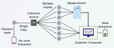
Fig. 1: Schematic of the possibilities for extracting work when a quantum system is prepared in some unknown state . We show that it is nearly impossible to extract any work with only a single copy of . On the other hand, when multiple copies are available, we provide a sample and qubit-efficient randomized quantum algorithm for work extraction that requires only a few samples of .
To estimate the maximal amount of extractable work by measuring ergotropy, it is necessary to optimize over unitaries , as shown in Eq. (1). The resulting optimal unitary depends on the spectrum of , which is revealed only when a complete description of the state of a quantum system is available. However, in realistic settings, due to technological limitations, the presence of uncontrollable environmental noise, and/or untrusted sources, the state in which the system is prepared is often unknown or, at best, only partially known [48, 49, 50, 51, 52, 53, 54, 55, 56, 57]. This makes it impossible to estimate ergotropy (and hence, the maximal possible extractable work) without performing a full tomography on , a highly inefficient procedure [58, 59]. The best we can hope for is to devise a strategy in such a black-box setting that still provides some information about the amount of extractable work while requiring only a few samples of . This naturally leads us to the following question: In such a black box setting, where the underlying quantum state is unknown, how many samples are needed to obtain an estimate of the amount of extractable work from the system? Despite the importance of a sample-efficient scheme for work extraction, this question has remained largely unexplored. In this paper, we address this gap by examining how the number of copies of affects work extraction.
One possibility is to proceed by assuming that the unknown state is random. Our first contribution is to rigorously establish that it is nearly impossible to extract any (non-zero) work from a single copy of the unknown random quantum state. This is obtained by proving that ergotropy is Lipschitz continuous with the Lipschitz constant scaling as the spectral norm of the Hamiltonian of the system, allowing us to use the concentration of measure phenomenon (such as Levy’s lemma [60]) to show that for any random , is close to its expectation value, which is zero. Owing to its connections with quantifying work, there is widespread interest in estimating ergotropy and understanding its properties. Consequently, our result is of independent interest. On the other hand, as mentioned before, tomography would require exponentially many samples and measurements to estimate ergotropy. This points to a trade-off between the number of available copies of the unknown state and extractable work. Interestingly, in Ref. [61], the authors propose a scheme using partial information from quantum measurements that quantifies the extractable work from unknown quantum states by associating it with a quantity called observational ergotropy. However, it is unclear if this quantity can be estimated faithfully in a sample-efficient manner.
Our second contribution equips this procedure with rigorous performance guarantees. More precisely, we develop a sample-efficient randomized protocol to estimate observational ergotropy, facilitating work extraction. Our method computes this quantity to -additive accuracy, with high probability, by making very few measurements on – this requires copies of and, remarkably, has only a logarithmic dependence on the dimension of the system. The protocol is a randomized quantum algorithm that can be efficiently run on a quantum computer using as many samples of . Our result thus broadens the applicability of quantum computers to the efficient estimation of extractable work and the characterization of quantum batteries.
Throughout this work, we consider -qubit quantum systems associated with a Hilbert space of dimension , and the underlying system is described by a Hamiltonian , which we have full knowledge of. Suppose denotes the set of density operators on , then, in our setting, the -qubit system of Hamiltonian is prepared in some unknown quantum state . Next, we discuss the two possible approaches to work extraction from (i) a single copy of , and (ii) multiple copies of (see Fig. 1).
(No) work extraction from a single copy of .— When only a single copy of the unknown state is available, it is, in principle, possible to consider to be a random state drawn from some statistical distribution over all possible density matrices. The idea would be to make use of the information about this distribution to extract some work. To this end, we assume that is a random density matrix whose purification leads to a Haar random state. We prove that it is almost always impossible to extract any nontrivial amount of work (ergotropy) with high probability over possible density matrices from this distribution. This result is obtained via a sequence of non-trivial steps, which we outline here, while detailed derivations can be found in Sec. B of the Appendix.
Since is a random quantum state, its ergotropy, , is a random variable. We first prove that the expectation value of this random variable, is zero. We then estimate for a random instance of how close is to its expected value. Typically, this is proved using measure concentration bounds, which requires Lipschitz continuity. However, whether the latter property holds for the ergotropy function has been unknown. We show ergotropy to be a Lipschitz continuous function with a Lipschitz constant of . This allows us to apply the concentration of measure bound to derive that with a high probability , for even exponentially small . Our results are formally stated via the following theorem.
Theorem 1(Impossibility of work extraction from a random state).
Let be a random state obtained by partial tracing subsystem of a randomly selected pure state with . Then, its ergotropy is a Lipschitz continuous function with Lipschitz constant . Moreover, for any ,
(2)
One expects that this limitation can be overcome given access to multiple copies of . Next, we explore the number of samples of required to quantify the amount of work that can be extracted from it.
Extracting work from multiple copies of .— We demonstrate that observational ergotropy, which characterizes work in such a black-box setting, can be estimated in a sample-efficient manner using a quantum computer. As outlined in Ref. [61], this quantity can be obtained via the following two-stage process: (i) Firstly, perform projective measurement with mutually orthogonal operators such that , and compute , for each . This step essentially decomposes the full space into blocks of orthogonal support, i.e. , where . We assume that the dimension of each block is , where . (ii) Secondly, randomize each block completely by applying a direct sum of Haar random unitaries to convert the still unknown state from the previous step into a known state . That is,
(3)
where is the normalized Haar measure, which factorizes nicely as . These steps allow us to compute , which is referred to as the observational ergotropy of the original unknown state [62, 63, 61]. That is,
(4)
where is a global unitary implementing a basis change from the basis of space to the eigenbasis of and a permutation that orders the ’s in non-increasing order. This has the effect of constructing the passive state with respect to , analogous to the role of the optimal unitary in the expression for ergotropy. As there is complete knowledge of , all that is required to construct are the ’s obtained from the first stage. Since is obtained by extracting partial information from the original state, the quantity provides a lower bound on , with the two quantities matching when is completely known.
We first quantify the number of samples of required to obtain an estimate of , for all . Performing a projective measurement results in outcome with probability . The strategy is to make repeated projective measurements, each time with a fresh copy of : for the iteration, the measurement outcome corresponds to an i.i.d. random variable whose expectation value is . So, for , we take the sample mean of each of the runs, i.e. . Then, Hoeffding’s inequality [64] ensures that , with a failure probability of at most , as long as
(5)
That is, if is the event that , then . Finally, the union-bound ensures that only samples are sufficient to ensure that for every , , with a probability of at least . Observe that the construction of the global unitary necessitates arranging the set of estimates in non-increasing order. That is, the accuracy with which these estimates approximate each should be such that they leave this ordering unaltered, i.e., should also imply , for all pairs of . Thus, if , this is ensured by choosing any . Despite requiring only a few measurements, this estimation scheme provides sufficient information regarding to enable the construction of . For detailed derivations, see Sec. C of the Appendix.
We are now in a position to estimate observational ergotropy for unknown . The central idea is to develop an easy-to-implement, efficient, randomized scheme that iteratively estimates the desired quantity. This is given by Protocol 1. Indeed, the outcome of this randomized protocol is a number that approximates the observational ergotropy to -additive accuracy, with a success probability of at least . We outline the details of this scheme.
1.
With probability , measure on the state .
2.
With probability , execute steps .
(a)
Measure in the basis spanned by the projectors and ignore the outcomes to obtain the post-measurement state .
(b)
Sample a unitary uniformly at random from the -qubit Pauli group, where , and apply the unitary to to obtain
(c)
Measure in the state obtained after Step 2(b).
3.
Store the outcome of the measurement of the iteration into .
4.
Repeat Steps 1 and 2, a total of times.
5.
Output .
Protocol 1
As the outcome of the measurement on is ignored, Step 2(a) naturally coarse grains the state. Note that each acts on the whole Hilbert space , but has support only on . If denotes the projection of on the support of , we have . It is easy to see that applying a direct sum of Haar random unitaries to this expected density matrix would result in the desired state (see Eq. (3)). However, implementing this efficiently is crucial to maintaining the sample efficiency of the overall protocol. For this, in Step 2(b), we sample uniformly at random a single unitary from the -qubit Pauli group , which is an exact -design of elements denoted as 111One could have also sampled from the -qubit Clifford group which is an exact -design [72, 73].. Note that
. Let be the (random) state after applying a uniformly sampled on , then the expected value of is given by
(6)
As discussed previously, applying the global unitary to this coarse-grained state would lead to the passive state corresponding to . Note that in Protocol 1, the outcome of a POVM measurement of in (Step 2(a)) is a random variable whose value lies in the interval , such that its expectation value is simply . Similarly, the outcome of Step 2(c) is another random variable with expectation value . As both these measurements are performed independently with probability , the outcome of the run of Steps 1 and 2 of Protocol 1 is a random variable such that .
Since these steps in Protocol 1 are executed a total of times, the outcome is a sequence of i.i.d. random variables . Finally, in Step 5, the overall output of our method is twice the mean of these random variables. We find for which the sample mean is an -accurate estimate of the actual expectation value () via Hoeffding’s inequality [64], which implies for any , . Thus, approximates observational ergotropy to -additive accuracy, i.e., , with probability at least , as long as
(7)
Overall, the probability estimation stage and the work estimation stage combined require samples (equivalently, as many measurements) of and succeeds with probability . Note that the overall sample complexity depends only logarithmically on the dimension of the system.
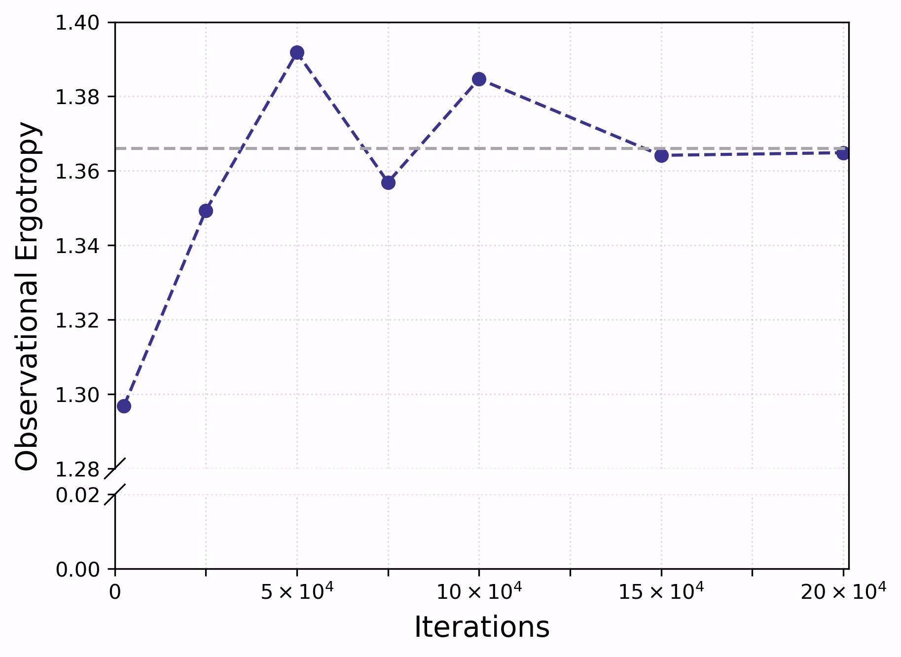
Fig. 2: Work extraction from translationally invariant Heisenberg XXX model. The Hamiltonian for spins is given by (with the periodic boundary condition), where and for Pauli- and Pauli- matrices for the th spin, respectively. For , let the spins be in the state , where . We have while . To estimate the latter quantity, we perform projective measurement with , , , and . The figure shows how Protocol 1 approximates as a function of the number of samples . For as in Eq. (7), we obtain an -accurate estimate of for , and failure probability .
In Fig. 2, we numerically demonstrate how Protocol 1 estimates the observational ergotropy. We plot this quantity as a function of samples of the unknown state. We consider a 3-qubit system described by the Heisenberg XXX model Hamiltonian [66]. For , , observe that Protocol 1 requires roughly samples to estimate the desired quantity. To help illustrate our findings, we provide other examples in Sec. E and Sec. F of the Appendix.
Our method can also be seen as a randomized quantum algorithm to estimate the amount of extractable work from an unknown state. Since the projectors are easily implementable, both stages can be implemented on a quantum computer requiring independent iterations. Interestingly, the quantum algorithm is qubit efficient, i.e., it requires no ancilla qubits and can potentially be implemented in the intermediate term. If is the circuit depth of the global unitary , then the circuit depth of each run is simply , as it requires constant circuit depth to implement a randomly sampled unitary from the -qubit Pauli group (in Step 2(b)). The precise depth of constructing is instance-specific: it depends on and the choice of the projective measurement , which determines the amount of coarse-graining. Note that this unitary implements (i) a basis change from the basis spanned by the projectors to the eigenbasis of the Hamiltonian, followed by (ii) a sequence of permutations required to arrange the estimated in non-increasing order. It is possible to implement (i) as is completely known, while the set of projectors is chosen by the user. Also, (ii) can be efficiently executed [67], with the gate depth depending on the number of permutations required to be implemented.
Our algorithm can be made more efficient in physically relevant settings. Observe that our scheme performs a measurement of on , which might be difficult to implement. However, consider any , which is a linear combination of -qubit Pauli strings with total weight . For such Hamiltonians, ubiquitous across physics [66], instead of measuring () in Step 1 (Step 2(c)) in each run of our algorithm, we can independently sample a Pauli term according to the ensemble and measure , and , respectively. It suffices to adopt this simple randomized measurement scheme, which enables the measurement of a single local Pauli operator in each run. In Sec. D of the Appendix, we prove that the modified Protocol 1 outputs which approximates to -additive accuracy, with probability at least as long as .
Discussion.— We consider the problem of extracting work from a physical system described by a known Hamiltonian but prepared in some unknown state . In this paper, we find the number of samples of required to estimate extractable work in such a black box setting. We prove that it is near impossible to extract any work from a single copy of . When multiple copies are available, we demonstrate that only samples suffice to estimate the amount of extractable work, as quantified by observational ergotropy, with a high success probability and -additive accuracy. The same number of samples of is then required to be leveraged as an energy source, e.g., for charging a quantum battery [68] or implementing an arbitrary quantum gate in an energy-efficient manner [69].
The value of observational ergotropy of depends on the choice of measurements and may even be non-positive in certain cases. In principle, it is possible to maximize this quantity over all possible measurement settings to ensure that it is non-negative. However, given practical constraints on the number of available copies, we restrict our analysis to only a single quantum measurement. It would be interesting to explore how multiple measurement settings would affect the sample complexity.
A subtle combination of randomized sampling and measurements is employed to ensure that our quantum algorithm for estimating extractable work is not only sample-efficient but also qubit-efficient. This is non-trivial as other ways of estimating observational ergotropy can be inefficient. In fact, in Sec. G of the Appendix, we show that more elaborate quantum algorithmic primitives, such as Linear Combination of Unitaries [70, 71] can be integrated into our scheme to estimate the extractable work. However, they increase the sample complexity exponentially and require ancilla qubits. Our work opens up avenues for future research on using quantum computers for estimating meaningful quantum thermodynamic quantities of physical systems, helping to build better, more resource-efficient quantum technological devices.
Acknowledgements.
We thank Hamed Mohammady for helpful comments. The authors acknowledge support from the Ministry of Electronics and Information Technology (MeitY), Government of India, under Grant No. 4(3)/2024-ITEA. AG and SD acknowledge support from the Science and Engineering Research Board, Department of Science and Technology (SERB-DST), Government of India, under Grant No. SRG/2023/000217. SC and SH acknowledge funding from the Science and Engineering Research Board, Department of Science and Technology (SERB-DST), Government of India under Grant No. SRG/2022/000354. SC also acknowledges funding from Fujitsu Ltd, Japan. SC, SD, and US thank IIIT Hyderabad for support via the Faculty Seed Grant.
References
Goold et al. [2016]J. Goold, M. Huber,
A. Riera, L. del Rio, and P. Skrzypczyk, The role of quantum information in
thermodynamics—a topical review, J. Phys. A: Math. Theor. 49, 143001 (2016).
Vinjanampathy and Anders [2016]S. Vinjanampathy and J. Anders, Quantum thermodynamics, Contemp. Phys. 57, 545 (2016).
Binder et al. [2018]F. Binder, L. A. Correa, C. Gogolin, J. Anders, and G. Adesso, eds., Thermodynamics in the Quantum Regime, Fundamental Theories of
Physics (Springer, Cham, Switzerland, 2018).
Deffner and Campbell [2019]S. Deffner and S. Campbell, Quantum Thermodynamics, 2053-2571 (Morgan & Claypool, Kentfield, CA, 2019).
Bera et al. [2019]M. N. Bera, A. Riera,
M. Lewenstein, Z. B. Khanian, and A. Winter, Thermodynamics as a Consequence of Information
Conservation, Quantum 3, 121 (2019).
Roßnagel et al. [2016]J. Roßnagel, S. T. Dawkins, K. N. Tolazzi, O. Abah,
E. Lutz, F. Schmidt-Kaler, and K. Singer, A single-atom heat engine, Science 352, 325 (2016).
Maslennikov et al. [2019]G. Maslennikov, S. Ding,
R. Hablützel, J. Gan, A. Roulet, S. Nimmrichter, J. Dai, V. Scarani, and D. Matsukevich, Quantum absorption
refrigerator with trapped ions, Nat. Commun. 10, 202 (2019).
Klatzow et al. [2019]J. Klatzow, J. N. Becker,
P. M. Ledingham, C. Weinzetl, K. T. Kaczmarek, D. J. Saunders, J. Nunn, I. A. Walmsley, R. Uzdin, and E. Poem, Experimental demonstration of quantum effects in the operation of
microscopic heat engines, Phys. Rev. Lett. 122, 110601 (2019).
Ferraro et al. [2018]D. Ferraro, M. Campisi,
G. M. Andolina, V. Pellegrini, and M. Polini, High-power collective charging of a solid-state quantum
battery, Phys. Rev. Lett. 120, 117702 (2018).
Yang et al. [2023]X. Yang, Y.-H. Yang,
M. Alimuddin, R. Salvia, S.-M. Fei, L.-M. Zhao, S. Nimmrichter, and M.-X. Luo, Battery
capacity of energy-storing quantum systems, Phys. Rev. Lett. 131, 030402 (2023).
Campaioli et al. [2024]F. Campaioli, S. Gherardini, J. Q. Quach, M. Polini, and G. M. Andolina, Colloquium: Quantum batteries, Rev. Mod. Phys. 96, 031001 (2024).
Scully et al. [2003]M. O. Scully, M. S. Zubairy,
G. S. Agarwal, and H. Walther, Extracting work from a single heat bath via
vanishing quantum coherence, Science 299, 862 (2003).
Horodecki and Oppenheim [2013]M. Horodecki and J. Oppenheim, Fundamental limitations
for quantum and nanoscale thermodynamics, Nat. Commun. 4, 2059 (2013).
Skrzypczyk et al. [2014]P. Skrzypczyk, A. J. Short, and S. Popescu, Work extraction and
thermodynamics for individual quantum systems, Nat. Commun. 5, 4185 (2014).
Singh et al. [2019]U. Singh, M. G. Jabbour,
Z. Van Herstraeten, and N. J. Cerf, Quantum thermodynamics in a multipartite setting:
A resource theory of local Gaussian work extraction for multimode bosonic
systems, Phys. Rev. A 100, 042104 (2019).
Pinto Silva and Gelbwaser-Klimovsky [2024]T. A. B. Pinto Silva and D. Gelbwaser-Klimovsky, Quantum work: Reconciling quantum mechanics and thermodynamics, Phys. Rev. Res. 6, L022036 (2024).
Acín et al. [2018]A. Acín, I. Bloch,
H. Buhrman, T. Calarco, C. Eichler, J. Eisert, D. Esteve, N. Gisin, S. J. Glaser, F. Jelezko, S. Kuhr,
M. Lewenstein, M. F. Riedel, P. O. Schmidt, R. Thew, A. Wallraff, I. Walmsley, and F. K. Wilhelm, The
quantum technologies roadmap: a european community view, New J. Phys. 20, 080201 (2018).
Buffoni et al. [2022]L. Buffoni, S. Gherardini,
E. Zambrini Cruzeiro, and Y. Omar, Third law of thermodynamics and the scaling of
quantum computers, Phys. Rev. Lett. 129, 150602 (2022).
Myers et al. [2022]N. M. Myers, O. Abah, and S. Deffner, Quantum thermodynamic devices: From theoretical
proposals to experimental reality, AVS Quantum Science 4, 027101 (2022).
Fellous-Asiani et al. [2023]M. Fellous-Asiani, J. H. Chai, Y. Thonnart,
H. K. Ng, R. S. Whitney, and A. Auffèves, Optimizing resource efficiencies for scalable full-stack
quantum computers, PRX Quantum 4, 040319 (2023).
Maillette de Buy Wenniger et al. [2023]I. Maillette de Buy Wenniger, S. E. Thomas, M. Maffei, S. C. Wein,
M. Pont, N. Belabas, S. Prasad, A. Harouri, A. Lemaître, I. Sagnes, N. Somaschi, A. Auffèves, and P. Senellart, Experimental analysis of energy transfers between a quantum emitter and
light fields, Phys. Rev. Lett. 131, 260401 (2023).
Moutinho et al. [2023]J. P. Moutinho, M. Pezzutto,
S. S. Pratapsi, F. F. da Silva, S. De Franceschi, S. Bose, A. T. Costa, and Y. Omar, Quantum
dynamics for energetic advantage in a charge-based classical full adder, PRX Energy 2, 033002 (2023).
Arrachea [2023]L. Arrachea, Energy dynamics, heat
production and heat–work conversion with qubits: toward the development of
quantum machines, Reports on Progress in Physics 86, 036501 (2023).
Jaschke and Montangero [2023]D. Jaschke and S. Montangero, Is quantum computing
green? an estimate for an energy-efficiency quantum advantage, Quantum Science and Technology 8, 025001 (2023).
Van Vu et al. [2024]T. Van Vu, T. Kuwahara, and K. Saito, Fidelity-dissipation relations in quantum
gates, Phys. Rev. Res. 6, 033225 (2024).
Majidi et al. [2024]D. Majidi, J. P. Bergfield, V. Maisi,
J. Höfer, H. Courtois, and C. B. Winkelmann, Heat transport at the nanoscale and ultralow
temperatures—implications for quantum technologies, Applied Physics Letters 124, 140504 (2024).
Lipka-Bartosik et al. [2024]P. Lipka-Bartosik, M. Perarnau-Llobet, and N. Brunner, Thermodynamic computing
via autonomous quantum thermal machines, Science Advances 10, eadm8792 (2024).
Lenard [1978]A. Lenard, Thermodynamical proof of
the Gibbs formula for elementary quantum systems, J. Stat. Phys. 19, 575 (1978).
Pusz and Woronowicz [1978]W. Pusz and S. L. Woronowicz, Passive states and kms
states for general quantum systems, Commun. Math. Phys. 58, 273 (1978).
Allahverdyan et al. [2004]A. E. Allahverdyan, R. Balian, and T. M. Nieuwenhuizen, Maximal work
extraction from finite quantum systems, Europhysics Letters 67, 565 (2004).
Singh et al. [2021]U. Singh, S. Das, and N. J. Cerf, Partial order on passive states and Hoffman
majorization in quantum thermodynamics, Phys. Rev. Research 3, 033091 (2021).
Sen and Sen [2021]K. Sen and U. Sen, Local passivity and entanglement in
shared quantum batteries, Phys. Rev. A 104, L030402 (2021).
Castellano et al. [2024]R. Castellano, D. Farina,
V. Giovannetti, and A. Acin, Extended local ergotropy, Phys. Rev. Lett. 133, 150402 (2024).
Bhattacharyya et al. [2024]A. Bhattacharyya, K. Sen, and U. Sen, Noncompletely positive quantum maps enable
efficient local energy extraction in batteries, Phys. Rev. Lett. 132, 240401 (2024).
Caves et al. [2002]C. M. Caves, C. A. Fuchs, and R. Schack, Unknown quantum states: The quantum
de Finetti representation, J. Math. Phys. 43, 4537 (2002).
Alvarez-Rodriguez et al. [2015]U. Alvarez-Rodriguez, M. Sanz, L. Lamata, and E. Solano, The forbidden quantum adder, Sci. Rep. 5, 11983 (2015).
Szangolies et al. [2015]J. Szangolies, H. Kampermann, and D. Bruß, Detecting entanglement of
unknown quantum states with random measurements, New J. Phys. 17, 113051 (2015).
Oszmaniec et al. [2016]M. Oszmaniec, A. Grudka,
M. Horodecki, and A. Wójcik, Creating a superposition of unknown quantum
states, Phys. Rev. Lett. 116, 110403 (2016).
Li et al. [2019]Z.-H. Li, M. Al-Amri,
X.-H. Yang, and M. S. Zubairy, Counterfactual exchange of unknown
quantum states, Phys. Rev. A 100, 022110 (2019).
Lebedev and Vinokur [2020]A. V. Lebedev and V. M. Vinokur, Time-reversal of an
unknown quantum state, Commun. Phys. 3, 129 (2020).
Cramer et al. [2010]M. Cramer, M. B. Plenio,
S. T. Flammia, R. Somma, D. Gross, S. D. Bartlett, O. Landon-Cardinal, D. Poulin, and Y.-K. Liu, Efficient
quantum state tomography, Nat. Commun. 1, 149 (2010).
Ledoux [2005]M. Ledoux, The Concentration of Measure Phenomenon, Mathematical Surveys and Monographs, Vol. 89 (American Mathematical Society, Providence, RI, 2005).
Šafránek et al. [2023]D. Šafránek, D. Rosa, and F. C. Binder, Work extraction from unknown quantum sources, Phys. Rev. Lett. 130, 210401 (2023).
Šafránek et al. [2019]D. Šafránek, J. M. Deutsch, and A. Aguirre, Quantum coarse-grained entropy and thermalization in closed
systems, Phys. Rev. A 99, 012103 (2019).
Šafránek et al. [2021]D. Šafránek, A. Aguirre, J. Schindler, and J. M. Deutsch, A brief introduction to observational
entropy, Foundations of Physics 51, 101 (2021).
Quek et al. [2024]Y. Quek, E. Kaur, and M. M. Wilde, Multivariate trace estimation in constant quantum
depth, Quantum 8, 1220 (2024).
Andolina et al. [2018]G. M. Andolina, D. Farina,
A. Mari, V. Pellegrini, V. Giovannetti, and M. Polini, Charger-mediated energy transfer in exactly solvable models for
quantum batteries, Phys. Rev. B 98, 205423 (2018).
Chiribella et al. [2021]G. Chiribella, Y. Yang, and R. Renner, Fundamental energy requirement of
reversible quantum operations, Phys. Rev. X 11, 021014 (2021).
Mele [2024]A. A. Mele, Introduction to Haar
Measure Tools in Quantum Information: A Beginner’s Tutorial, Quantum 8, 1340 (2024).
Narasimhachar and Gour [2015]V. Narasimhachar and G. Gour, Low-temperature
thermodynamics with quantum coherence, Nature Communications 6, 7689 (2015).
Zyczkowski and Sommers [2001]K. Zyczkowski and H.-J. Sommers, Induced measures in the
space of mixed quantum states, J. Phys. A: Math. Gen. 34, 7111 (2001).
Zyczkowski and Sommers [2003]K. Zyczkowski and H.-J. Sommers, Hilbert–schmidt volume
of the set of mixed quantum states, J. Phys. A: Math. Gen. 36, 10115 (2003).
Hall [1998]M. J. W. Hall, Random quantum
correlations and density operator distributions, Phys. Lett. A 242, 123 (1998).
Raginsky and Sason [2013]M. Raginsky and I. Sason, Concentration of measure
inequalities in information theory, communications, and coding, Found. Trends Commun. Inf. Theory 10, 1 (2013).
Berry et al. [2015]D. W. Berry, A. M. Childs,
R. Cleve, R. Kothari, and R. D. Somma, Simulating hamiltonian dynamics with a truncated taylor series, Phys. Rev. Lett. 114, 090502 (2015).
Childs et al. [2017]A. M. Childs, R. Kothari, and R. D. Somma, Quantum algorithm for systems of
linear equations with exponentially improved dependence on precision, SIAM Journal on Computing 46, 1920 (2017).
Chakraborty et al. [2019]S. Chakraborty, A. Gilyén, and S. Jeffery, The Power of
Block-Encoded Matrix Powers: Improved Regression Techniques via Faster
Hamiltonian Simulation, in 46th International Colloquium on Automata, Languages, and Programming (ICALP
2019), Leibniz International Proceedings in
Informatics (LIPIcs), Vol. 132, edited by C. Baier,
I. Chatzigiannakis,
P. Flocchini, and S. Leonardi (Schloss Dagstuhl – Leibniz-Zentrum für Informatik, Dagstuhl, Germany, 2019) pp. 33:1–33:14.
van Apeldoorn et al. [2020]J. van
Apeldoorn, A. Gilyén, S. Gribling, and R. de Wolf, Quantum SDP-Solvers:
Better upper and lower bounds, Quantum 4, 230 (2020).
Appendix
In the Appendix, we introduce preliminaries and provide detailed proofs of some of the unproven statements in the main article. We also give additional examples that illustrate the sample complexity of our work extraction algorithm. Finally, an ancilla-assisted work extraction protocol is also discussed, which, although interesting, results in a worse sample complexity than our protocol in the main text.
Appendix A Preliminaries – Work extraction and ergotropy
Recall that , the Hilbert space of qubits is denoted by and the set of density operators, trace one positive semi-definite matrices, on is denoted by . Further, define . The Hamiltonian of the qubit system, denoted by , satisfies
(8)
where is the projector onto the eigensubspace of energy , is the degeneracy of the energy eigenvalue , and for all . is the total number of distinct eigenvalues of and . Let us further define an ordering on the eigenstates, for convenience, as follows: . Denote by the ordered tuple of eigenvectors arranged in order of nondecreasing energy. Here we have partitioned as such that . In particular, the set
spans the eigenspace of energy , where .
Ergotropy:–Let us consider a quantum system of qubits with the Hamiltonian (Eq. (8)) in an arbitrary state . Note that the extractable work is a path/process dependent quantity; the extractable work from any quantum system can be defined in multiple ways depending on the quantum operations used for work extraction (see, e.g., Refs. [38, 22, 74, 25]). Ergotropy is a notion of extractable work under unitary operations. The ergotropy of a quantum system in a state is defined as [38, 40]
(9)
where is the group of unitary matrices. Let the spectral decomposition of be given by , where and . Let be the permutation of objects such that for all . Then the unitary matrix achieving the maximum in Eq. (9) can be written as
(10)
Thus, ergotropy of the state can be written as
(11)
For the nondegenerate Hamiltonian, i.e., (with ), the above expression simplifies to
(12)
Observational ergotropy:– For a physical system described by Hamiltonian on , the observational ergotropy of a state is defined with respect to a measurement setting. Consider the projective measurement described by projectors such that , and , for all . Then, the observational ergotropy of is defined as
(13)
where , for . If is the same for all , is a global unitary that implements (i) a basis change from to the eigenbasis of , followed by (ii) a permutation that orders the ’s in non-increasing order. We refer the readers to Refs. [62, 63, 61] for the bounds on observational ergotropy and other details.
Appendix B Concentration of ergotropy
B.1 Induced measures on the space of mixed states
The notion of random states requires a probability measure to be associated with the set of states. For an -dimensional system with Hilbert space , a random pure state may be written as , where is a fixed pure state and is an unitary matrix chosen uniformly from the unique Haar measure on the unitary group (see e.g. Refs. [75, 76]).
However, the set of density matrices (nonnegative and trace one matrices) does not admit any unique probability measure on it, and in fact, there exist several inequivalent measures on . For example, one may generate a random density matrix by partial tracing the purifications chosen uniformly from the unique Haar measure on the pure states in , where . This procedure induces the probability measure on the eigenvalues
of , which is given by [76, 77]
(14)
where is the normalization constant and . The eigenvectors of are distributed via the unique Haar measure on . The normalized probability measure over is then given by
(15)
where , .
Another way to obtain a probability measure on is to note that any density matrix , using the spectral decomposition theorem, can be written as , where is an unitary matrix and is a diagonal matrix with nonnegative real entries that sum to one. Then assuming that the distributions of eigenvalues and eigenvectors of are independent, one may propose a probability measure on as , where the measure is the unique Haar measure on and measure defines the distribution of eigenvalues (see e.g. Refs. [78, 76]). The measure is not unique and one may pick it based on different metrics on the Hilbert space [79]. In particular, for Hilbert-Schmidt metric, coincides with given in Eq. (15) [76]. In this work, we will focus only on the partial trace induced measure on the set of density matrices.
B.2 Lipschitz continuity and the concentration of measure phenomenon
Lipschitz continuity:– Let and be two metric spaces with metrics and , respectively and be a function on . Then is said to be a Lipschitz continuous function with the Lipschitz constant if for any
(16)
Note that any other constant is also a valid Lipschitz constant [80, 60, 81]. One can obtain a Lipschitz constant for function as [82, 83]
(17)
Concentration of measure phenomenon:– Certain smooth functions defined over measurable vector spaces are known to take values close to their
average values almost surely [60]. This phenomenon is collectively referred to as the concentration of measure phenomenon and is expressed via various inequalities bounding the probability of departure of the functional values from the average value. Logarithmic Sobolev inequalities together with the Herbst argument (also called the “entropy method”) are very general techniques to prove such inequalities [82]. A particular form of the concentration inequality suitable for our exposition is stated as the following lemma [80, 60, 83, 84].
Lemma 1(Concentration of measure phenomenon).
Let be the -sphere and be the set of real numbers. Let be a Lipschitz continuous function with Lipschitz constant . Then for each point chosen at random and for , we have
(18)
where and is the measure on .
Average ergotropy:–Let be a random state in obtained via partial tracing Haar random pure states on , where and , be an arbitrary state. The ergotropy of is given by . Let the maximization be obtained at . Then
(19)
Since is a random state, is a random variable. In the following lemma, we show that the expectation value of is vanishing.
Lemma 2.
The average ergotropy is zero for random quantum states sampled from the distribution (Eq. (15)).
Proof.
We have
(20)
In the third line above, we used the left invariance of the Haar measure.
∎
We now have all the ingredients to prove that is a Lipschitz continuous function. We state our results via the following lemma:
Lemma 3.
The ergotropy of quantum states is a Lipschitz continuous function with Lipschitz constant . That is, for such that and , where is an -dimensional system, we have
(21)
Proof.
Let be a density matrix in such that , where is an -dimensional system. Here is a pure state in a composite Hilbert space of dimension and is the eigenbasis of the Hamiltonian of the system while is some orthogonal basis for the system . Let be such that for . Due to the normalization condition, , all pure states lie on -sphere . Let us define a function as . Then
(22)
Using above, we have
(23)
Then
(24)
where is the operator norm of , which is equal to the maximum eigenvalue of . Thus, using Eq. (17), the Lipschitz constant corresponding to the function is given by . That is, for any two pure states and , we have
(25)
Let
us define a function as . Let be the spectral decomposition of such that for . Then the minimization in above equation is achieved for the unitary . Then
(26)
Now
(27)
Similarly,
(28)
Then
(29)
Thus, using Eq. (17), the Lipschitz constant corresponding to the function is given by . That is, for any two pure states and , we have
(30)
Now using Eqs. (25) and (30) we can estimate the Lipschitz constant for ergotropy as follows.
(31)
This completes the proof of the lemma.
∎
Finally, we prove Theorem 1, the main result of this section:
Theorem 2(Concentration of ergotropy).
Let be a random density matrix obtained by partial tracing randomly selected pure state in a composite Hilbert space of dimension of . Then the probability that ergotropy of is slightly away from zero is close to zero for large . In particular, for each , we have
(32)
Proof.
The proof of the theorem follows by applying Lemma 1 to the ergotropy function with and noting that the average ergotropy is zero (see Lemma 2). Further, ergotropy is a Lipschitz continuous function with Lipschitz constant (see Lemma 3).
∎
Appendix C Hoeffding inequality and probability estimation
Let us consider independent and identically distributed (i.i.d.) random variables which satisfy . Let, for all , . For such i.i.d. random variables, for all , Hoeffding’s inequality [64, 85] states that
(33)
Let be an unknown -qubit quantum state, and we want to estimate probabilities of outcomes of a projective measurement given by such that and for all . Further, , where . Suppose we perform this projective measurement times. At each instance of measurement, the outcome is one of the indices . Let us define an indicator function , which is one if the measurement outcome is and zero otherwise. During th repetition of the measurement, we store the value of in the random variable . The expectation value of for each is given by , where for . Then, defining , from Hoeffding’s inequality for i.i.d. random variables , for all we have
(34)
where we used the fact that for each and . Now, for , by choosing or
(35)
we have . Thus, samples of suffice to estimate within additive error and maximum failure probability . Now applying union bound on measurement outcomes , we have
(36)
where denotes the event that . This implies that samples of are sufficient to estimate for all within additive error and maximum failure probability .
Choosing the error : As discussed in the main article, the estimates need to be arranged in non-increasing order for the construction of the global unitary . It is thus necessary to ensure that the precision is such that it does not alter the ordering of the original ’s. In other words, we intend to find error in the estimated probabilities such that implies for all pairs . For the equality case, i.e., , the error incurred in estimation does not affect . Now, for distinct pairs let us define . Then for , we have . Using this, we have
Thus, taking (e.g. taking ), we can ensure that the error incurred in the estimation of probabilities does not affect the choice of global unitary. These choices imply the following lemma.
Lemma 4.
The number of samples of required to estimate probabilities upto an error , i.e., for all with failure probability at most can be taken as
(37)
where .
The proof of Lemma 4 follows directly by substituting the upper bound on into the expression for . This shows that the estimation of probabilities for all with additive error and failure probability at most requires only samples of the unknown state.
Appendix D Randomized quantum algorithm for work extraction from local Hamiltonians
For this section, consider any -qubit Hamiltonian
where each is a string of -qubit Pauli operators and . Without loss of generality, we assume that . This is because, in general, these coefficients can be written as , where . In this case, the imaginary phase can be absorbed into the description of the Pauli operator itself, i.e., .
In this case, we can replace the POVM measurements of in Protocol 1 with the measurements of randomly sampled which takes values in . These modifications simplify the measurement scheme while still ensuring that the randomized algorithm estimates observational ergotropy to -additive accuracy, with a success probability of at least . We outline the steps via Protocol 2.
1.
With probability , sample and measure on the state .
2.
With probability , execute steps .
(a)
Measure in the basis spanned by the projectors and ignore the outcomes to obtain the post-measurement state .
(b)
Sample a unitary uniformly at random from the -qubit Pauli group, where , and apply the unitary to to obtain
(c)
Sample and measure in the state obtained after step (b) above.
3.
Store the outcome of the measurement of the iteration into .
4.
Repeat Steps 1 and 2(a)-(c), a total of times.
5.
Output .
Protocol 2Work Extraction from local Hamiltonians
In particular, Step 1 and Step 2(c) of Protocol 1 is modified as follows: instead of measuring (or ), sample a Pauli string according to the ensemble , and perform a POVM measurement of with respect to in Step 1 (or equivalently in Step 2(c)). Note that , and the iteration of Steps 1, and Steps 2(a)-(c) in Protocol 2 results in a random variable in Step 3 such that
Then, the overall output of Protocol 2 (Step 5) is
As before, Hoeffding’s inequality ensures that
So, we have
with probability as long as
Appendix E Example of a -qubit system
Let us consider a -qubit system with the Hamiltonian
(38)
where . Here and . The spectral decomposition of this Hamiltonian is given by , where
Further let with . Consider the unknown state to be , where
(39)
The energy of state is given by .
A minimum energy state (such a state is not unique here) with respect to is given by
(40)
The energy of state is given by . The ergotropy of is given by
E.1 Measurement in entangled basis
Let the projective measurement be given by , where for , where
(41)
(42)
(43)
(44)
Indeed all ’s are two dimensional projectors and in fact , , , and , where , , , and .
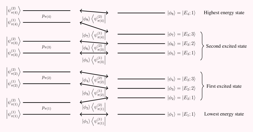
Fig. 3: The schematic above shows the action of global unitary on measured state to yield a corresponding passive state for and Hamiltonian given by Eq. (38). Let the projective measurement be given by , where and . Let be the unknown state and . Let be the permutation on objects such that for all . Then we define .
Let us now compute the probabilities . We have , , , and . The average state after the measurement is given by . The energy is given by . The eigenvalues of are given by . The minimum energy state corresponding to this state is given by
(45)
The ergotropy of the state is given by
After averaging with respect to Haar measure, we get . The energy of the state is given by . The eigenvalues (in decreasing order) and the corresponding set of eigenvectors of are given by
Let us define permutation as , i.e., . Using this, let us consider a global unitary (see Fig. 3)
The minimum energy state for is then given by
(46)
The ergotropy of the state is given by .
while the observational ergotropy of the state is given by (See Table 1 and Fig. 4a).
Table 1: Ergotropy and observational ergotropy. For state , where , , and are given in Eq. (39), the table shows values of ergotropy and observational ergotropy for two different measurement settings.
(a) Measurement in entangled basis
(b) Measurement in product basis
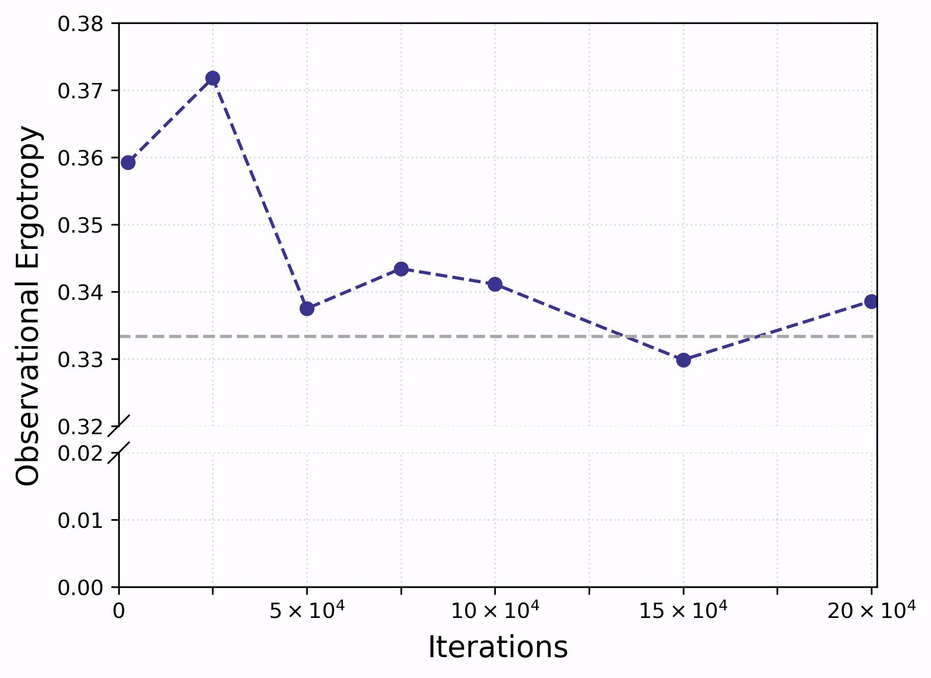
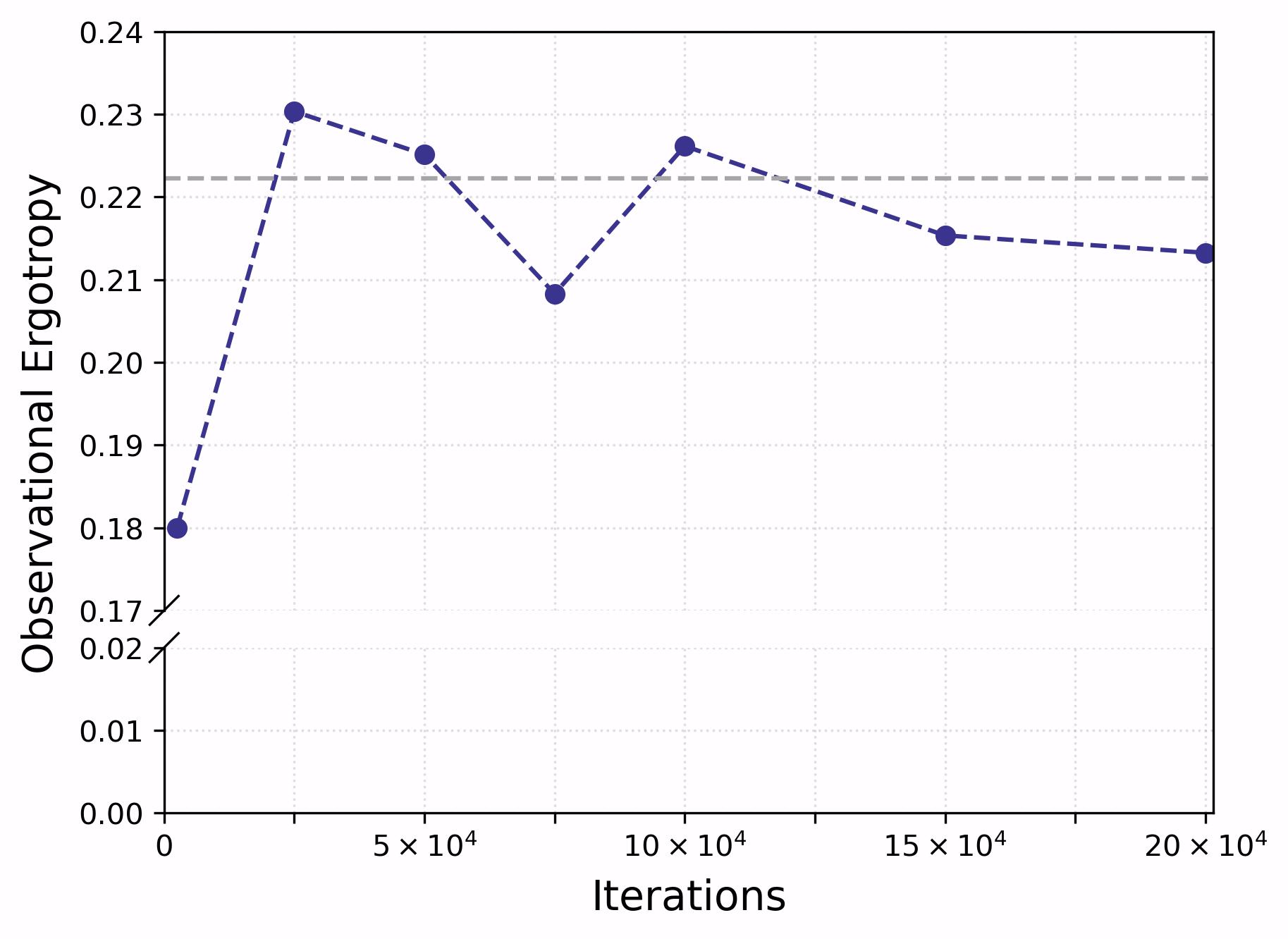
Fig. 4: Observational ergotropy and sample complexity. Consider a state , where , , and are given in Eq. (39). Figs. (4a) and (4b) show the convergence of our protocol from main text to the exact value of observational ergotropy, as we increase number of samples, with respect to measurements in entangled (Sec. E.1) and product (Sec. E.2) bases, respectively.
E.2 Measurement in product basis
Let the projective measurement be given by , where , , , and .
We have , , , and . The average state after the measurement is given by . The energy is given by . The eigenvalues of are given by . The minimum energy state corresponding to this state is given by
(47)
The ergotropy of the state is given by . After averaging wrt to Haar measure, we get
(48)
The energy of the state is given by . The minimum energy state for is given by
(49)
The energy of the state is given by . The ergotropy of the state is given by . The observational ergotropy of the state is given by (See Table 1 and Fig. 4b).
Appendix F Example of qubit translationally invariant spin chain
In this section we consider translationally invariant spin chain, in particular, one dimensional Heisenberg XXX model, as an example. For spins such a spin chain is described by the Hamiltonian
(50)
where is the spin coupling constant, is the transverse magnetic field and the periodic boundary condition is ensured by identification .
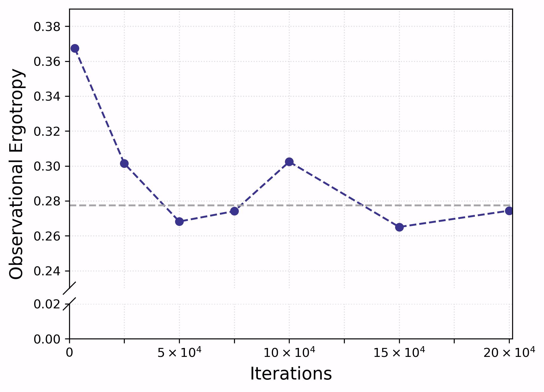
Fig. 5: Heisenberg XXX model. For the state in Eq. (51), the exact observational ergotropy of is equal to . The figure shows how our protocol for work extraction reaches to as we increase the number of samples in accordance with the bound on the sample complexity.
The sign of ensures whether the ground state is ferromagnetic or antiferromagnetic [86, 87, 88]. Here we take and . For the case of spins, we consider the state
(51)
where , and
(52)
The ergotropy of is computed to be . Further, to obtain observational ergotropy, we perform the projective measurement defined by the projectors for , where
(53)
With the above projectors, the observational ergotropy of is given by . In Fig. 5, we show how our protocol reaches this value as we increase the number of samples.
Appendix G Estimating observational ergotropy using Linear Combination of Unitaries
In this section, we discuss a different approach for estimating observational ergotropy. It is, in principle, possible to use a different sampling strategy to implement a direct sum of Haar random matrices in Protocol 1. For this, we express this quantity (which is itself a unitary) as a Linear Combination of Unitaries (LCU) [70]. Observe that can be expressed as as a linear combination of unitaries as follows:
where is a diagonal unitary matrix and for all . The matrices above are unitaries and are defined as
(54)
Even though this framework has been central to the development of a number of near-optimal quantum algorithms [70, 89, 90, 91, 92], it is quite resource-demanding as it requires several ancilla qubits and multi-qubit controlled operations to be implemented. However, recently, a randomized quantum algorithm for LCU was introduced [91], which requires circuits of shorter depth and only a single ancilla qubit. So, instead of randomly sampling an element from the -qubit Pauli group as described in Protocol 1, we can implement by using the Single-Ancilla LCU algorithm of Ref. [91]. However, we prove that this leads to a substantial increase in the sample complexity.
Let us first consider a unitary -design of cardinality on the spaces whose dimensions are the same for all . Here , for all , are unitaries acting on for all . Further, let us define a set of cardinality as follows.
(55)
In the following lemma we prove that is itself a unitary -design on .
Lemma 5.
The set , Eq. (55), of direct sums of unitaries on Hilbert spaces for sampled from a unitary -design constitute a unitary -design on with respect to the product measure.
Proof.
Note that averaging of an unknown state with respect to sampled from the Haar measure produces
(56)
where and is the dimension of the each block on which is the projector. Now consider , is sampled from a unitary -design of cardinality . Further, let the elements of be given by with . Each is of the form . To prove the lemma, it is sufficient to prove that
(57)
where is a projector for all and . We analyze the cases in Eq. (G), separately.
For the case: In this case, the action of on corresponds to applying a unitary on the subspace defined by the projector . For each choice of in a given subspace we can have possible choices of in remaining subspaces. This means that for each block we will have . Now we have
(58)
where .
For the case: For , the action of on corresponds to applying two unitaries: from left on block and from right on block . Given any two choices of in the and block, respectively, of we can have possible choices of in the remaining blocks of . In particular, we have
With probability , perform energy measurement on unknown state .
2.
With probability , execute steps to .
(a)
Prepare the state .
(b)
Sample an integer uniformly at random from to select .
(c)
Obtain i.i.d. samples from the distribution .
(d)
Define and . Obtain the state from as
Perform measurement of on the state .
(e)
Multiply to the measurement outcome.
3.
For the iteration, store the outcome , which on an average (as Steps and occur with probability each) takes value , where and .
4.
Repeat Steps to for times to obtain values and output .
Protocol 3Work Extraction using Single-Ancilla LCU
Integrated sampling strategy:–We sample from the Pauli group of elements. This set then naturally induces the set of elements (see Eq. (54)). There are such sets , let us denote them by for . Thus, in Protocol 3, we can effectively do the following: sample an integer uniformly at random to select the set . Now, we can proceed by obtaining i.i.d. samples according to the ensemble . Then by following the steps of Protocol 3, we output some such that for any observable ,
(60)
where . We can formally state the steps of Protocol 3.
Remark 1.
In step 1 of Protocol 3, the outcomes for the measurement of are the eigenvalues of . In step 2(d), when we are measuring , for each eigenvalue of , there are two possible outcomes of , namely, .
Theorem 3.
Suppose . Let be an -qubit Hamiltonian and be an -dimensional unknown density matrix. Then Protocol 3 outputs satisfying,
with success probability at least for
(61)
Further, if the unitary can be constructed with gate depth and is the upper bound on the gate depth of the most expensive , the cost of each run is at most .
Proof.
In each run of the protocol, with probability , protocol measures (see Eq. (8)) in the state . This results in an outcome with probability , where . Step , with probability , performs measurement of on the state , where
In the expression for , and are unitaries sampled with probability each indirectly from , which itself is sampled with probability . Simplifying , we have
We have , where and . Thus, measurement in step results in outcome with probability for fixed and . Each run of steps and of the Protocol 3 results in an independent and identically distributed random variable. Let us call this random variable and it takes values with probability and with probability for fixed and . That is, for all . This also implies that . The expectation value of is given by
where ,
and denotes the trace with respect to first system. Further, . Thus, we have
where and is given by Eq. (3). But the protocol gives us the sample average, i.e, instead of . The random variable takes values in the interval . Now, applying Hoeffding’s inequality to , we have
Thus, taking
ensures that
Thus, it is sufficient to choose
to estimate the observational egrotropy with an additive error and success probability at least for all and .
∎
As mentioned previously, the sample complexity is exponentially worse than Protocol 1 of the main article as the factor can scale as a polynomial in the dimension .