Design of thermal meta-structures made of functionally graded materials using isogeometric density-based topology optimization

Abstract

The thermal conductivity of Functionally Graded Materials (FGMs) can be efficiently designed through topology optimization to obtain thermal meta-structures that actively steer the heat flow. Compared to conventional analytical design methods, topology optimization allows handling arbitrary geometries, boundary conditions and design requirements; and producing alternate designs for non-unique problems. Additionally, as far as the design of meta-structures is concerned, topology optimization does not need intuition-based coordinate transformation or the form invariance of governing equations, as in the case of transformation thermotics. We explore isogeometric density-based topology optimization in the continuous setting, which perfectly aligns with FGMs. In this formulation, the density field, geometry and solution of the governing equations are parameterized using non-uniform rational basis spline entities. Accordingly, the heat conduction problem is solved using Isogeometric Analysis. We design various 2D & 3D thermal meta-structures under different design scenarios to showcase the effectiveness and versatility of our approach. We also design thermal meta-structures based on architected cellular materials, a special class of FGMs, using their empirical material laws calculated via numerical homogenization.

1 Introduction

1.1 Thermal metamaterials and meta-structures

By controlling heat flow, the thermal analogues of electrical devices can be created, such as resistors, capacitors, inductors, diodes and transistors. In addition, new thermal detection-anti-detection, computing and communication devices can be developed. Despite its significance, storing and steering heat is not an easy task as there are multiple modes of heat transfer and the heat transfer processes are intrinsically less ordered than ballistic/wave transport. In recent years, thermal metamaterials have emerged as a tool to manipulate and control heat transfer [1, 2, 3, 4]. Thanks to their architected structures, thermal metamaterials can achieve thermal properties, which are difficult to find in natural materials.

Traditionally, these metamaterials are mainly designed by the analytical methods, such as transformation thermotics [5, 6, 7] and the scattering cancellation method [8, 9]. Using these methods, several thermal metamaterials have already been proposed and experimentally demonstrated, such as thermal cloak, thermal concentrator, thermal rotator and thermal expander [7, 10, 11, 1]. However, these design methods are only efficient with limited regular geometries under specific design conditions. They face difficulties handling any arbitrary design scenario mainly due to their analytical nature. Transformation thermotics also requires an intuition-based coordinate transformation, which is not easy to devise. Moreover, often deduced thermal property distributions are (extremely) anisotropic and heterogeneous; and therefore difficult to manufacture.

To overcome the above-mentioned limitations, a numerical method could be an effective alternative. As designing metamaterials/meta-structures is essentially an inverse problem, one can exploit structural optimization methods as a design tool. At first, Dede et al. [12, 13] designed thermal composites for heat flux shielding, focusing and reversal using topology optimization. Following it, several other articles focusing on the usage of optimization to design thermal meta-structures [14, 15, 16, 17, 18, 19, 20, 21]. Hirasawa et al. [22] experimentally demonstrated optimization-based thermal cloaking meta-structures. Similarly, we also aspire to utilize the structural optimization for designing thermal meta-structures to achieve versatility and flexibility in handling arbitrary geometries and design conditions.

In our earlier works [23, 24], we used shape optimization and (a more flexible) topology optimization to design thermal meta-structures. Both methods focus on distributing natural constituent materials at the macroscale to produce an apparent effect of required anisotropy and heterogeneity for thermal metamaterials/meta-structures. Though these methods are effective in their respective design spaces, their design spaces are limited by a few discrete conductivities. At times, to achieve an apparent anisotropy and heterogeneity, the methods can produce designs with intricate material distributions that are challenging to manufacture as observed for thermal camouflages (without regularization), as discussed in [24]. In this paper, we contemplate enlarging the design spaces by including functionally graded materials in the design. We could think of this as distributing the constituents at a smaller scale rather than the macroscale. Correspondingly, we propose thermal meta-structures made of functionally graded materials.

1.2 Functionally Graded Materials

Functionally Graded Materials (FGMs) is a new class of materials characterized by the gradual variation of properties across the volume through variation in structure, microstructure or composition [25, 26]. With this definition, the functionally graded porous/lattice structures or Architected Cellular Materials (ACMs), with structural variations occurring at a smaller scale than the scale of observation, can also be included in the family of FGMs. In FGMs, smooth gradations in properties can be beneficial for reducing residual stresses or stress concentration and therefore, interfacial separation and cracking. Recent advances in additive manufacturing made the manufacturing of FGMs easier compared to expensive and time-consuming conventional manufacturing processes [27, 28, 29]. From a constructive perspective, the material gradation can be accurately tailored to design desired heterogeneity, which is often a primary requirement of a thermal meta-structure. Therefore, utilizing an FGM in thermal meta-structure design is a straightforward logical approach.

1.3 Topology optimization

Topology optimization is a structural optimization method that focuses on optimizing the connectivity, shape, and placement of voids within a given design domain. Topology optimization has several variants such as (1) density-based approach [30, 31, 32], (2) level-set method [33, 34, 35] (3) phase field approach [36] and (4) evolutionary algorithm approach [37] (5) Moving Morphable Component (MMC)/Moving Morphable Void (MMV)/Geometric Projection (GP) approach [38, 39, 40, 41]. For more detailed information about all approaches, interested readers can refer to the following articles [42, 43, 44, 45, 46, 47]. Among different methods, density-based and level-set methods have remained the most popular ones. The density-based approaches consider the continuous material formulation and behave as a sizing problem in terms of density [30, 31, 32, 48]. Commonly, they employ a penalization scheme, such as the Solid Isotropic Material with Penalization (SIMP) and the Rational Approximation for Material Properties (RAMP), that penalizes the intermediate densities to achieve the discrete designs. However, the continuous framework of the density-based approach without penalization perfectly aligns with FGMs whose peculiarity is a continuous gradation in composition/structure.

As an early work on topology optimization of FGMs, Paulino et al. [49] proposed so-called FGM-SIMP formulation to design FGM structures. They employed the continuous approximation of material distribution (CAMD) for density field parameterization and corresponding nodal densities as the design variables. Later, Almeida et al. [50] studied the effect of global and local level gradation in the topology optimization of FGMs. The level-set method is also explored in the context of FGMs by Xia et al. [51]. Even functionally graded cellular/porous structures are designed using topology optimization in the following articles [52, 53, 54, 55]. Taheri and his collaborators published several articles [56, 57, 58] on a fully isogeometric structural optimization for optimizing eigen-frequency, thermoelastic stress and compliance, respectively. In their fully isogeometric structural optimization approaches, density, geometry and solution field were parameterized using the same non-uniform rational b-splines (NURBS) basis functions and accordingly, Isogeometric Analysis (IGA) [59, 60] was employed to solve the boundary value problems.

In this article, we too exploit fully NURBS-based density topology optimization with the NURBS-parameterized density, geometry and solution fields as in [56]. The NURBS-parameterised density provides quite a few advantages over element-wise densities or nodal densities as utilized in [61, 62, 56]; getting inherent filtering effect against the checker-boarding issue, obtaining smoother material distributions, straight forward calculation of derivatives of density, providing complete cost-effective analytical sensitivities. The fully NURBS-based topology optimization formulation holds the potential to build an integrated design-analysis-optimization model with its tightly integrated design field-to-geometry and geometry-to-solution-field mappings. Moreover, IGA offers advantages over the classical finite element method (FEM) by enabling the exact representation of conic geometries, handling higher inter-element continuity and providing higher efficiency for higher-order elements [59, 60]. The detailed literature related to isogeometric optimization approaches can be found in the review articles [63, 64].

1.4 Contribution of the present study

In the present study, we design thermal meta-structures made of FGMs using isogeometric density topology optimization. In summary, the key features of this paper are:

• Design of thermal meta-structures made of FGMs and ACMs: In this article, we designed thermal meta-structures made of FGMs. We explored both analytical and experimental homogenization models for thermal conductivity. We also showcased thermal meta-structures made of ACMs using an empirical material law established on numerical homogenization results. Following it, the reconstruction of an entire cellular structure based on the optimization results is presented too.

• Versatile and more flexible design tool than the conventional analytical methods: In our article, we showcased that the proposed approach can effectively design thermal meta-structures with arbitrary geometries, boundary conditions, design constraints/regularizations and objective functions. It can also generate alternative designs for the design problems which lacks uniqueness such as thermal cloak probelm [65, 66, 67] with simple modifications.

• Fully NURBS-based formulation: By using a fully NURBS-based topology optimization, the proposed method provides inbuilt filtering, smoother material distributions, straightforward calculation of density gradient and closed-form sensitivities, higher inter-element continuity, exact geometric representation (for conic geometries) and higher numerical efficiency for the higher-order elements. It also has the potential for building an integrated design-analysis-optimization model.

• Verification and comparison: We verified our topology optimization-based tool by designing various 2D & 3D thermal meta-structures found in literature such as thermal cloaks, thermal concentrators, thermal rotators, thermal cloaked sensors, multi-functional thermal meta-structures (thermal cloak concentrator), and multi-directional thermal meta-structure (thermal horizontal concentrator- vertical cloak). As the most of literature results are achieved using a different methodology (and does not involve FGMs), it is difficult to provide a quantitative comparison with our results. Yet, we tries to offer a qualitative comparison for some special cases of thermal cloaks and thermal concentrators.

The remainder of the paper is organized as follows: Section 2 describes the boundary value problem and numerical formulation to solve it. Section 3 describes various models to calculate the effective thermal conductivity of FGMs that are utilized in our work. The optimization problem and sensitivity analysis are explained in Section 4. In Section 5, thermal cloaks are designed in various design scenarios to showcase the effectiveness of the proposed method. Section 6 explores other thermal meta-structures and corresponding different objective functions. Section 7 briefly covers the reconstruction process of Architected Cellular Materials (ACMs) designed using topology optimization. Lastly, Section 8 presents the conclusions and some prospects of the current work.

2 Boundary value problem

2.1 Problem description

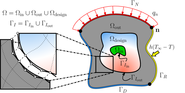
Figure 1: Domain description of the boundary value problem. $\Omega_{\rm design}$ represents a design region where thermal meta-structure is optimized, $\Omega_{\rm in}~\&~\Omega_{\rm out}$ are the inside and outside regions with respect to $\Omega_{\rm design}$, respectively. $\Omega$=$\Omega_{\rm in}\cup\Omega_{\rm out}\cup\Omega_{\rm design}$. $\Gamma=\partial\Omega=\Gamma_{D}\cup\Gamma_{N}\cup\Gamma_{R}$. The solid black line shows an explicitly defined interfaces $\Gamma_{I_{\rm in}}$ and $\Gamma_{I_{\rm out}}$, $\Gamma_{I}=\Gamma_{I_{\rm in}}\cup\Gamma_{I_{\rm out}}$. The square is shown in detail highlighting the matching of control points of connecting patches at the interface $\Gamma_{I}$.

Let us consider an FGM-based thermal meta-structure distributed across $\mathrm{\Omega}_{\rm design}$, which is embedded in the homogeneous isotropic domain $\mathrm{\Omega}\in\mathbb{R}^{d},d\in\{{2,3}\}$. The inside and outside regions are denoted as $\mathrm{\Omega}_{\rm in}$ and $\mathrm{\Omega}_{\rm out}$, respectively. $\mathrm{\Omega}=\mathrm{\Omega}_{\rm in}\cup\mathrm{\Omega}_{\rm design}\cup\mathrm{\Omega}_{\rm out}$. The external boundary $\mathrm{\Gamma}=\partial\mathrm{\Omega}$ is decomposed into three parts $\mathrm{\Gamma}_{D}$, $\mathrm{\Gamma}_{N}$ and $\mathrm{\Gamma}_{R}$, $\mathrm{\Gamma}=\mathrm{\Gamma}_{D}\cup\mathrm{\Gamma}_{N}\cup\mathrm{\Gamma}_{R}$. On $\mathrm{\Gamma}_{D}$, $\mathrm{\Gamma}_{N}$ and $\mathrm{\Gamma}_{R}$, the Dirichlet, Neumann and Robin boundary conditions are applied, respectively. Moreover, internal boundaries $\mathrm{\Gamma}_{I_{\rm in}}$ & $\mathrm{\Gamma}_{I_{\rm out}}$ separate $\mathrm{\Omega}_{\rm in}$ and $\mathrm{\Omega}_{\rm out}$ from $\mathrm{\Omega}_{\rm design}$, respectively. Internal boundaries are denoted as $\mathrm{\Gamma}_{I}$, $\mathrm{\Gamma}_{I}=\mathrm{\Gamma}_{I_{\rm in}}\cup\mathrm{\Gamma}_{I_{\rm out}}$. The 2D domain description is shown in Figure 1. For the given arrangement, the steady-state heat conduction boundary value problem with an internal heat generation $q_{b}$ in the temperature field $T$ is given as:

$$\nabla\cdot\left(\bm{\kappa}(v)\nabla T\right)+q_{b} =0,\quad \textrm{in}\quad\mathrm{\Omega},$$ (1a)

$$T =T_{D},\quad \textrm{on}\quad\mathrm{\Gamma}_{D},$$ (1b)

$$(\bm{\kappa}(v)\nabla T)\cdot\mathbf{n} =q_{n},\quad \textrm{on}\quad\mathrm{\Gamma}_{N},$$ (1c)

$$(\bm{\kappa}(v)\nabla T)\cdot\mathbf{n} =h(T_{\infty}-T),\quad \textrm{on}\quad\mathrm{\Gamma}_{R},$$ (1d)

where $\nabla$ is the gradient operator, $q_{n}$ is the flux applied on $\mathrm{\Gamma}_{N}$, $T_{D}$ is the prescribed temperature on $\mathrm{\Gamma}_{D}$, $\mathbf{n}$ is the unit normal on the boundary, $\bm{\kappa}$ is the thermal conductivity matrix, $h$ is the heat transfer coefficient, $T_{\infty}$ is the bulk temperature.

As our thermal meta-structure is made of FGM, the (macroscopic) thermal conductivity matrix varies point-wise. The thermal conductivity variation is governed by the variation of compositions/structures at a smaller scale. These microstructure variations are homogenized using an appropriate homogenization law to calculate an effective macroscopic property. Possibly, the effective macroscopic property can be defined as a function of several microstructure parameters. For a fixed type of unit cell, the microstructure parameters could be reduced to the volume fractions/relative densities of the constituents. In our case, we only consider FGMs made of two constituents (or one constituent in the case of an FGM characterized by structural variation with porosity being the other constituent) with a fixed-type unit cell. Therefore, the effective thermal conductivity is written as a function of the relative density $v$ of filler material/porosity, i.e., $v=V/V_{0}$, $V$ being the volume of filler material/porosity in the unit cell and $V_{0}$ being the total volume of the unit cell. The relative density of the other constituent will be $1-v$. Consequently, the current work focuses on optimizing this relative density distribution. Various models to calculate the effective thermal conductivity are presented in Section 3. Other regions $\Omega_{\rm in}$ and $\Omega_{\rm out}$ are also assumed to be filled with homogeneous isotropic materials. Note that the materials constituting the unit cell of the FGM are isotropic. Nevertheless, the equivalent homogeneous material replacing the unit cell at the macroscopic scale exhibits a cubic syngony behaviour. That being the case, the conductivity matrix can be easily defined as $\bm{\kappa}(v)=\kappa(v)\mathbf{I}_{d}$ with $\mathbf{I}_{d}$ being an identity matrix in $\mathbb{R}^{d}$. The conductivities of homogeneous materials are included in the functional form via constant functions.

Across the internal interfaces $\mathrm{\Gamma}_{I_{\rm in}}$ and $\mathrm{\Gamma}_{I_{\rm out}}$, the temperature and normal flux are assumed to be continuous. If the connected regions at $\mathrm{\Gamma}_{I}$ are denoted by indices 1 and 2 locally, the interface boundary conditions are written as:

$$\left\llbracket T\right\rrbracket \coloneqq T^{1}-T^{2}=0,\quad \textrm{on}\quad\mathrm{\Gamma}_{I},$$ (2a)

$$\mathbf{n}\cdot\left\llbracket\bm{\kappa}(v)\nabla T\right\rrbracket \coloneqq\mathbf{n}^{1}\cdot\bm{\kappa}^{1}(v^{1})\nabla T^{1}+\mathbf{n}^{2}\cdot\bm{\kappa}^{2}(v^{2})\nabla T^{2}=0,\quad \textrm{on}\quad\mathrm{\Gamma}_{I},$$ (2b)

where $\llbracket\cdot\rrbracket$ is the jump operator and $\mathbf{n}=\mathbf{n}^{1}=-\mathbf{n}^{2}$.

2.2 Solution of the boundary value problem using IGA

To solve the boundary value problem, the strong form described in Eq. (1) is transformed into the weak form using the standard Bubnov-Galerkin formulation. The interface conditions mentioned in Eq. (2) are also incorporated in the weak formulation using Nitsche’s method [68, 69]. At last, the modified Bubnov-Galerkin weak formulation is given as follows: Find $T^{h}\in\mathscr{T}^{h}\subseteq\mathscr{T}=\big{\{}T\in\mathbb{H}^{1}({\mathrm{\Omega}}),T=T_{D}\hskip 4.26773pt\textrm{on}\ {\mathrm{\Gamma}}_{D}\big{\}}$ such that $\forall S^{h}\in\mathscr{S}^{h}_{0}\subseteq\mathscr{S}_{0}=\left\{S\in\mathbb{H}^{1}({\mathrm{\Omega}}),S=0\hskip 4.26773pt\textrm{on}\ {\mathrm{\Gamma}}_{D}\right\}$,

$$a(T^{h},S^{h},v)=\ell(S^{h}),$$ (3)

with

$$a(T^{h},S^{h},v)=\int_{\mathrm{\Omega}}(\nabla S^{h})^{\rm T}\bm{\kappa}(v)\nabla T^{h}d\mathrm{\Omega}-\int_{\mathrm{\Gamma}_{I}}\left(\mathbf{n}\cdot\{\bm{\kappa}(v)\nabla S^{h}\}\right)^{\rm T}\llbracket T^{h}\rrbracket~d\mathrm{\Gamma}\\ -\int_{\mathrm{\Gamma}_{I}}\llbracket S^{h}\rrbracket^{\rm T}\left(\mathbf{n}\cdot\{\bm{\kappa}(v)\nabla T^{h}\}\right)d\mathrm{\Gamma}+\int_{\mathrm{\Gamma}_{I}}\beta~\llbracket S^{h}\rrbracket^{\rm T}\llbracket T^{h}\rrbracket~d\mathrm{\Gamma}+\int_{\mathrm{\Gamma}_{R}}h(S^{h})^{\rm T}~T^{h}~d\mathrm{\Gamma},$$ (4a)

$$\ell{(S^{h})}=\int_{\mathrm{\Omega}}(S^{h})^{\rm T}q_{b}~d\mathrm{\Omega}+\int_{\mathrm{\Gamma}_{N}}(S^{h})^{\rm T}q_{n}~d\mathrm{\Gamma}+\int_{\mathrm{\Gamma}_{R}}(S^{h})^{\rm T}hT_{\infty}~d\mathrm{\Gamma},$$ (4b)

where $\beta$ is the stabilization parameter and $\{\cdot\}$ is the averaging operator defined as $\{\theta\}=\gamma\theta^{1}+(1-\gamma)\theta^{2}$ with $\gamma$ being the averaging parameter ($0<\gamma<1$). for the current work, $\beta=1\times 10^{12}$ and $\gamma=0.5$. In the literature [68, 69], it is reported that the large stabilization parameter might cause ill-conditioning of the system, but we did not face any conditioning issues for our boundary value problem. The verification of the accuracy of Nitsche’s method is performed in our earlier work on shape optimization [23].

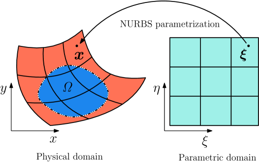
Figure 2: Parametrization of a point from the parametric domain to a point in the physical domain using NURBS basis functions.

As we are exploiting IGA for approximation, the geometry, test function and trial function are parameterized using NURBS basis functions. If $n$ NURBS $N_{i}$, $i=1,2,...,n$ are employed to discretize the weak form, these approximations are written as:

$$\bm{x}(\bm{\xi})=\sum_{i=1}^{n}\mathbf{X}_{i}N_{i}(\bm{\xi}),\quad T^{h}(\bm{\xi})=\sum_{i=1}^{n}T_{i}N_{i}(\bm{\xi}),\quad\textrm{and}\quad S^{h}(\bm{\xi})=\sum_{i=1}^{n}S_{i}N_{i}(\bm{\xi}),$$ (5)

where $\bm{x}$ is a physical point in $\Omega$, and $\bm{\xi}$ is the corresponding parametric point as shown in Figure 2, $\mathbf{X}_{i}$ is the $i^{th}$ control point and $T_{i}$ & $S_{i}$ are corresponding temperature & arbitrary temperature. By substituting these approximations in Eq. (3), we can obtain a linear matrix system as follows:

$$\mathbf{K}\mathbf{T}=\mathbf{F},$$ (6)

where $\mathbf{K}$ is the global stiffness matrix, $\mathbf{F}$ is the global force vector and $\mathbf{T}$ is the vector of temperature at control points. A detailed derivation of matrix formulation is given in A.

3 Models for effective thermal conductivity of functionally graded materials

For analysis of FGMs using numerical methods such as FEM, an accurate model of the material property gradation is crucial to ensure numerical accuracy. In earlier works of FEM, material properties were assumed to remain constant across each element. With element-wise constant properties, FEM requires a fine mesh and thus higher computational effort to represent a smooth gradation. To overcome this limitation, Santare et al. [70] proposed a graded finite element approach to analyze heterogeneous materials like FGMs. In this approach, the material properties are sampled directly at the integration points using explicit functions. Later, Kim et al. gave a generalized isoparametric FEM formulation [71], where material properties are sampled at nodes of finite elements. The properties inside the elements were interpolated using the same shape functions as geometry and solution field. A generalized IGA formulation was also proposed by Tahiri et al. [58]. Other works on numerical analysis of FGMs can be found in [72, 73, 74, 75, 76]. As we are working on optimizing the relative density, the thermal conductivity is directly sampled at integration points using the relative density values similar to [70].

The effective thermal conductivity tensor as a function of the relative density of the FGMs at the macroscopic scale is assessed through a dedicated homogenization method. Several homogenization models have been proposed to estimate the effective thermal conductivity [77] for heterogeneous materials. Generally, these models stem from different analytical and numerical homogenization techniques. Analytical homogenization schemes are mostly based on micro-mechanics models and may be valid for specific composite materials [77, 78, 79]. Their accuracy critically depends on parameters such as matrix-filler conductivities; dimensions, shape, orientation and dispersion pattern of filler materials. On the other hand, numerical homogenization schemes are more general and based on finite element simulations of Representative Volume Element (RVE)/unit-cell [80, 81, 82]. Numerical schemes face difficulties in the realistic modelling of material behaviour, interface-boundary conditions and fillers. Often, numerical schemes are computationally expensive due to the need for a large number of simulations across various configurations of RVEs and a fine mesh in each simulation to capture the features of fillers.

In this article, to demonstrate the universality across several types of material laws, we exploit a total of six material models, covering three distinct types : micro-mechanics models, empirical models based on experimental data, and empirical models based on numerical homogenization of graded lattice structures. The discussed models and the chosen constituent materials are detailed in the next few paragraphs. Formulæ to find the effective thermal conductivity $\kappa_{\rm eff}$, limits on the relative density values, i.e., $v$-range ([$v_{\rm min},v_{\rm max}$]) and corresponding limits on the effective thermal conductivity, i.e., $\kappa_{\rm eff}$-range ([$\kappa_{\rm min},\kappa_{\rm max}$]) of the considered models are reported in Table 1. We also plot the effective thermal conductivity $\kappa_{\rm eff}$ and its derivative with respect to the relative density $v$ in Figure 3.

Regarding analytical models, we explored two well-known models named Effective Medium Theory (EMT) and Maxwell model [79, 77]. We consider copper ($\kappa_{\rm copper}=398$ W/mK) and Polydimethylsiloxane (PDMS) ($\kappa_{\rm PDMS}=0.27$ W/mK) as the constituents. By considering one higher conductivity material and one lower conductivity material, we aim to exploit a wider range of thermal conductivity for design and hence a larger design space. From the manufacturing perspective, very limited research can be found on FGMs made of highly contrasting thermal conductivities. Therefore, it is difficult to comment on the manufacturability of these FGMs. We also apply purely theoretical limits on relative density $v$, $v_{\rm min}=0$ & $v_{\rm max}=1$.

Model name	Effective thermal conductivity ($\kappa_{\rm eff}$)	$v$ - range	$\kappa_{\rm eff}$ - range (in W/mK)
Micromechanics models ($\kappa_{m}$ is thermal conductivity of a matrix material, $\kappa_{i}$ is thermal conductivity of a filler; here, $\kappa_{m}=\kappa_{\rm copper}=398$ W/mK and $\kappa_{i}=\kappa_{\rm PDMS}=0.27$ W/mK)
Effective Medium Theory (EMT) [79]	$\kappa_{\rm eff}=\dfrac{1}{4}\left(\tau+\sqrt{\tau^{2}+8\kappa_{i}\kappa_{m}}\right)$  with $\tau=(3v-1)\kappa_{i}+\left(3(1-v)-1\right)\kappa_{m}$	[0, 1]	[0.27, 398]
Maxwell [79]	$\kappa_{\rm eff}=\kappa_{m}\dfrac{2\kappa_{m}+\kappa_{p}-2v(\kappa_{m}-\kappa_{p})}{2\kappa_{m}+\kappa_{p}+v(\kappa_{m}-\kappa_{p})}$	[0, 1]	[0.27, 398]
Empirical models based on experimental data ($\kappa_{m}=\kappa_{\rm copper}=398$ W/mK)
Lotus type porous copper [83]	$\kappa_{\rm eff}=\kappa_{m}\dfrac{1-v}{1+v}$	[0, 0.7]	[70.24, 398]
Cu-Sn-Pb composite [84]	$\kappa_{\rm eff}=\kappa_{m}\left(ae^{bv}+ce^{dv}\right))$ $a=9.34008\times 10^{-1}$, $b=-2.81400\times 10^{1}$, $c=7.08923\times 10^{-2}$, $d=1.14783\times 10^{-3}$	[0, 0.3]	[28.31, 399.95]
Empirical models based on numerical homogenization of graded lattice structure (of copper), ($\kappa_{m}=\kappa_{\rm copper}=398$ W/mK)
Truncated CubOctaHedron (TCOH) [53]	$\kappa_{\rm eff}=\kappa_{m}\sum\limits_{i=1}^{7}C_{i}v^{i}$, $C_{1}=0.4231$, $C_{2}=0.1236$, $C_{3}=0.0933$, $C_{4}=0.0902$, $C_{5}=0.0899$, $C_{6}=0.0899$, $C_{7}=0.0899$	[0.2, 0.8]	[36.01, 228.52]
Gyroid [53]	$\kappa_{\rm eff}=\kappa_{m}\sum\limits_{i=1}^{7}C_{i}v^{i}$, $C_{1}=0.5934$, $C_{2}=0.1119$, $C_{3}=0.0631$, $C_{4}=0.0583$, $C_{5}=0.0578$, $C_{6}=0.0577$, $C_{7}=0.0577$	[0.2, 0.9]	[7.13, 397.96]

Table 1: Various effective thermal conductivity models considered for the FGMs.

Next, we explore the empirical models of thermal conductivity based on experimental data. We refer to the effective thermal conductivity data of lotus-type porous copper and composite of Cu-Sn-Pb taken from Ogushi et al. [83] and Mercuri et al. [84], respectively. For the lotus-type porous copper, the empirical model is already established in [83], and we are utilizing the same model. As for Cu-Sn-Pb, we extracted the data from [84] and fitted a curve using MATLAB curve fitting toolbox [85]. The limits on relative density $v$ are also imported from the reference articles.

At last, we explore the numerical homogenization results of graded ACMs [86, 53, 54, 55]. ACMs are often used in thermal applications due to their improved heat transfer due to their high surface-to-mass ratio. ACMs have a predefined unit cell, whose geometric features are directly linked to the relative density. Therefore, their numerical homogenization can be performed offline prior to the optimization, and its results can be used as the empirical model for effective thermal conductivity. Nonetheless, to ensure the accuracy of the numerical homogenization during optimization, the scale separation hypothesis must be satisfied. The scale separation hypothesis [87] assumes that the characteristic dimensions of the periodic unit cells in the lattice are much smaller than the characteristic dimensions of the entire structure & phenomena. At last, the multiscale structure can be reconstructed based on optimized density distribution through the reconstruction process [53, 88]. More details about ACMs and their design using optimization can be found in [86, 88].

Some of the commonly used unit cells for ACMs are Strut-like lattices and Triply Periodic Minimal Surface (TPMS) lattices. We chose two unit-cells called Truncated CubOctaHedron (TCOH) & Thin Walled Gyroid. Their numerical homogenization data and their empirical models published in Montemurro et al. [53] are utilized. Both models are presented in terms of the relative density of porosity. For TCOH, $v_{\rm min}=0.2$ & $v_{\rm max}=0.8$ are taken considering the manufacturing constraints. As for Gyroid, $v_{\rm min}=0$ & $v_{\rm max}=0.97$ are possible as the feasible limits mentioned in Li et al. [54]. Nevertheless, we take slightly conservative limits of $v_{\rm min}=0.2$ and $v_{\rm max}=0.9$ into account.

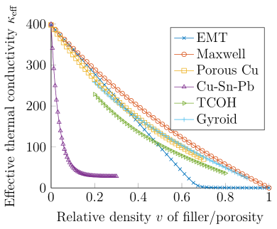
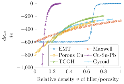
Figure 3: Effective thermal conductivity $\kappa_{\rm eff}$ and its derivative with respect to the relative density $v$ for all models shown in Table 1.

4 Optimization problem

4.1 Density field parameterization

As pointed out in the introduction section, we use the NURBS basis functions to parameterize the density field. The parameterized density field using $m$ NURBS basis functions $R_{i}$ can be given as:

$$v(\bm{\xi})=\sum_{i=1}^{m}R_{i}(\bm{\xi})v_{i},$$ (7)

with

$$\nabla v(\bm{\xi})=\sum_{i=1}^{m}\nabla R_{i}(\bm{\xi})v_{i},$$ (8)

where $v_{i}$ is the relative density corresponding to the $i^{th}$ control point. The density values at control points are utilized as the design variables. Note that the weights associated with the control points are predefined (based on the geometry and coordinates of control points). These values do change during optimization, as the weights are not considered as the design variables.

Often, due to the NURBS having support spanning multiple knot spans, the NURBS-based parameterization provides an inherent filtering effect that can prevent checker-boarding issues. In addition, the gradients of the density field would be given by a straightforward formula, as shown in Eq. (8), which could simplify the employment of density-based restrictions in the optimization problem. In the case of the element-wise density field, one of the reasons for checker-boarding is the inter-element discontinuity. This discontinuity also makes the calculation of density field gradient difficult. Alternatively, the nodal density field (with the so-called continuous approximation of material distribution using Lagrange basis functions) provides limited $C^{0}$ inter-element continuity. It is well-known that the higher-order elements are quite effective against checker-boarding. However, the higher-order Lagrange elements cannot be straightforwardly implemented due to their non-negativity property. Hence, the NURBS-based density parameterization is quite beneficial compared to other common alternatives.

As evident from Eq. (7), the choice of density parameterization defines the design freedom. A finer NURBS mesh for density means more design variables, and thereby a larger optimization problem and higher associated computational cost. For this reason, it is beneficial to decouple both design and solution parameterizations. By decoupling, we ensure satisfactory solution accuracy by refining solution parameterization without increasing the size of the optimization problem. For future, it would also be interesting to decouple geometry and solution field parameterizations in addition to design and solution field parameterizations [89]. Geometric Independent Field approximaTion (GIFT), proposed by Atroshchenko et al.[90], offers such independence between geometry and solution field parameterizations in IGA framework. By decoupling the geometry and solution fields, we can exploit locally refined splines such as T-splines and PHT-splines for solution field parameterization [91], to take advantage of local refinement, without disturbing the geometry parameterization.

4.2 Optimization problem

Next, we formulate the optimization problem based on the given design parameterization. Suppose $\mathbf{V}=[v_{1}\hskip 6.99997ptv_{2}\hskip 6.99997pt...\hskip 6.99997ptv_{N_{\rm var}}]^{\rm T}$ is the vector of the $N_{\mathrm{var}}$ design variables, and $J$ is the objective function. In the most general case, $N_{\text{var}}$ can be different from the number of control points of the design mesh $m$ in Eq. (7) depending on applied symmetry. The isogeometric density topology optimization problem for a thermal meta-structure can be defined as:

$$\min_{\mathbf{V}\in\mathbb{R}^{N_{\mathrm{var}}}}~J(T^{h},v),$$ (9)

with

$$J:\mathbb{R}^{N_{\mathrm{var}}}\rightarrow\mathbb{R},$$ (10a)

$$J:\mathbf{V}\rightarrow J(T^{h}(\mathbf{V}),v(\mathbf{V})),$$ (10b)

such that the following constraints are satisfied,

Equality constraints: $$h_{i}(T^{h}(\mathbf{V}),v(\mathbf{V}))=0,\quad i=1,2,...,N_{h},$$ (11)

Inequality constraints: $$g_{j}(T^{h}(\mathbf{V}),v(\mathbf{V}))\leq 0,\quad i=1,2,...,N_{g},$$ (12)

Box constraints: $$v_{i,\rm min}\leq~v_{i}\leq~v_{i,\rm max}\quad i=1,2,...,N_{\mathrm{var}},$$ (13)

where $N_{h}$ and $N_{g}$ are the number of equality constraints and inequality constraints, respectively. $v_{i,\rm min}$ and $v_{i,\rm max}$ are lower and upper bounds of the design variable $v_{i}$. For our numerical examples, we will have at least two equality constraints related to the boundary value problem as given below,

Equality constraint: $$a(T^{h},S^{h},v)=\ell(S^{h}),\forall S^{h}\in\mathscr{S}^{h}_{0}\quad \textrm{in}\quad\Omega,$$ (14)

Equality constraint: $$T=T_{D}\quad \textrm{on}\quad\Gamma_{D},$$ (15)

However, these equality constraints are satisfied explicitly by solving the linear system for evaluating temperature $T$ at each optimization iteration.

The given optimization problem is then solved using Sequential Quadratic programming (SQP) algorithm. A nonlinear mathematical programming technique like SQP has sophisticated step selection and constraint handling strategies, in addition to optimized speed and efficiency. As we implement the methodology in MATLAB, its ‘fmincon’ optimization toolbox with the ‘sqp’ subroutine is directly used for straightforwardness [92]. Also, since SQP algorithm is a gradient-based algorithm, both objective function and constraint sensitivities with respect to design variables are required to update the values of the design variables at each iteration. The required sensitivities are calculated using the adjoint method [93] and fed to the algorithm. The next subsection will outline the procedure to evaluate the objective function and constraint sensitivities.

4.3 Sensitivity analysis

The adjoint method [93] to calculate sensitivity is described in this subsection. In the most general case, we define the objective function $J(T,v)$ of a thermal meta-structure as a sum of a domain integral and a surface integral as follows:

$$J(T,v)=\int_{\Omega_{J}}J_{b}(T,v)~d\Omega+\int_{\Gamma_{J}}J_{s}(T,v)~d\Gamma,$$ (16)

where ${\Omega_{J}}$ is the domain where the domain integral is calculated, and ${\Gamma_{J}}$ is the boundary where the surface integral is calculated.

In order to find the objective function sensitivities, the Lagrangian $\mathcal{L}$ is defined as:

$$\mathcal{L}:\underbrace{\mathbb{H}^{1}(\mathbb{R}^{2})}_{T}\times\underbrace{\mathbb{H}^{1}(\mathbb{R}^{2})}_{P_{J}}\times\underbrace{\mathbb{H}^{1}(\mathbb{R}^{2})}_{v}\times\underbrace{\mathbb{H}^{1}(\mathbb{R}^{2})}_{\lambda}\rightarrow\mathbb{R},$$ (17)

with

$$\mathcal{L}(T,P_{J},v,\lambda)=J(T,v)+\ell(P_{J})-a(T,P_{J},v)+\int_{\mathrm{\Gamma}_{D}}\lambda(T-T_{D})~d\mathrm{\Gamma},$$ (18)

where $P_{J}$ and $\lambda$ are the Lagrange multipliers of the weak form as well as Dirichlet boundary condition as defined in Eqs. (14)-(15).

The optimality conditions of the minimization problem are derived as the stationary conditions of the Lagrangian. The stationary conditions with respect to $\lambda$ and $P_{J}$ give back the weak formulation of the boundary value problem as stated in Eq. (3), which can be satisfied by solving the matrix system given in Eq. (6) for the state variable $T$. The stationary condition with respect to $T$,

$$\left<\dfrac{\partial\mathcal{L}(T,P,\varPhi,\lambda)}{\partial T},\delta T\right>=0,$$ (19)

combined with the Dirichlet boundary condition, gives a well-posed adjoint problem as follows:

$$\nabla\cdot\left(\bm{\kappa}\nabla P_{J}\right) =\dfrac{\partial J(T,v)}{\partial T}\quad \textrm{in}\quad\mathrm{\Omega},$$ (20a)

$$P_{J} =0\quad \textrm{on}\quad\mathrm{\Gamma}_{D},$$ (20b)

$$(\bm{\kappa}(v)\nabla P_{J})\cdot\mathbf{n} =0\quad \textrm{on}\quad\mathrm{\Gamma}_{N},$$ (20c)

$$(\bm{\kappa}(v)\nabla P_{J})\cdot\mathbf{n} =-hP_{J},\quad \textrm{on}\quad\mathrm{\Gamma}_{R},$$ (20d)

$$\left\llbracket P_{J}\right\rrbracket =0\quad \textrm{on}\quad\mathrm{\Gamma}_{I},$$ (20e)

$$\mathbf{n}\cdot\left\llbracket\bm{\kappa}\nabla P_{J}\right\rrbracket =0\quad \textrm{on}\quad\mathrm{\Gamma}_{I},$$ (20f)

where $P_{J}$ is the adjoint temperature field. By employing the trial and test function approximations, the adjoint problem can be written in the matrix form as:

$$\mathbf{K}^{\rm T}\mathbf{P}_{J}=\mathbf{F}_{J},$$ (21)

where $\mathbf{P}_{J}$ is the vector of adjoint temperatures at control points, $\mathbf{F}_{J}$ is the global adjoint flux vector defined as:

$$\mathbf{F}_{J}=\int_{\Omega_{J}}\mathbf{N}^{\textrm{T}}\dfrac{\partial J_{b}}{\partial T}~d\Omega+\int_{\Gamma_{J}}\mathbf{N}^{\textrm{T}}\dfrac{\partial J_{s}}{\partial T}~d\Gamma,$$ (22)

At last, with the fulfillment of all three stationary conditions, the sensitivity of the objective function $\left({dJ}/{dv_{i}}\right)$ becomes equal to the total derivative of Lagrangian $\mathcal{L}$ with respect to a design variable $v_{i}$. Therefore:

$$\dfrac{dJ}{dv_{i}}=\int_{\Omega_{J}}\dfrac{\partial J_{b}}{\partial v}~\dfrac{dv}{dv_{i}}~d\Omega+\int_{\Gamma_{J}}\dfrac{\partial J_{s}}{\partial v}~\dfrac{dv}{dv_{i}}~d\Gamma-(\mathbf{P}_{J})^{\rm T}~\dfrac{d\mathbf{K}}{dv}~\dfrac{dv}{dv_{i}}~\mathbf{T}.$$ (23)

By applying the density parameterization from Eq. (7), the sensitivity equation can be simplified as:

$$\dfrac{dJ}{dv_{i}}=\int_{\Omega_{J}}\dfrac{\partial J_{b}}{\partial v}~R_{i}~d\Omega+\int_{\Gamma_{J}}\dfrac{\partial J_{s}}{\partial v}~R_{i}~d\Gamma-(\mathbf{P}_{J})^{\rm T}~\dfrac{d\mathbf{K}}{dv}~R_{i}~\mathbf{T}.$$ (24)

A derivative of the global stiffness matrix $\mathbf{K}$ with respect to relative density $v$ is provided in A. The first and second terms in Eq. (24) are related to the explicit dependency of the objective function on relative density, while the last term is related to its dependency on relative density via the state variable, i.e., the temperature $T$.

With the same procedure, the constraint sensitivities can be formulated too. In our case, we define a generalized equality constraint $h$ and a generalized inequality constraint $g$ in a similar manner to the objective function by the summation of a domain integral and a surface integral as follows:

$$h(T,v)=\int_{\Omega_{h}}h_{b}(T,v)~d\Omega+\int_{\Gamma_{h}}h_{s}(T,v)~d\Gamma,$$ (25)

$$g(T,v)=\int_{\Omega_{g}}g_{b}(T,v)~d\Omega+\int_{\Gamma_{g}}g_{s}(T,v)~d\Gamma,$$ (26)

where $\Omega_{h},\Gamma_{h},h_{b},h_{s}$ & $\Omega_{g},\Gamma_{g},g_{b},g_{s}$ are equality and inequality constraints related quantities following the nomenclature analogous to the objective function as described earlier in the section. Accordingly, the constraint sensitivities are defined as:

$$\dfrac{dh}{dv_{i}}=\int_{\Omega_{h}}\dfrac{\partial h_{b}}{\partial v}~R_{i}~d\Omega+\int_{\Gamma_{h}}\dfrac{\partial h_{s}}{\partial v}~R_{i}~d\Gamma-(\mathbf{P}_{h})^{\rm T}~\dfrac{d\mathbf{K}}{dv}~R_{i}~\mathbf{T},$$ (27)

$$\dfrac{dg}{dv_{i}}=\int_{\Omega_{g}}\dfrac{\partial g_{b}}{\partial v}~R_{i}~d\Omega+\int_{\Gamma_{g}}\dfrac{\partial g_{s}}{\partial v}~R_{i}~d\Gamma-(\mathbf{P}_{g})^{\rm T}~\dfrac{d\mathbf{K}}{dv}~R_{i}~\mathbf{T}.$$ (28)

Corresponding adjoint temperature vectors $\mathbf{P}_{h}$ and $\mathbf{P}_{g}$ are obtained by solving extra adjoint systems similar to Eq. (21) with the global adjoint flux vectors $\mathbf{F}_{h}$ & $\mathbf{F}_{g}$ given as follows:

$$\mathbf{F}_{h}=\int_{\Omega_{h}}\mathbf{N}^{\textrm{T}}\dfrac{\partial h_{b}}{\partial T}~d\Omega+\int_{\Gamma_{h}}\mathbf{N}^{\textrm{T}}\dfrac{\partial h_{s}}{\partial T}~d\Gamma,$$ (29)

$$\mathbf{F}_{g}=\int_{\Omega_{g}}\mathbf{N}^{\textrm{T}}\dfrac{\partial g_{b}}{\partial T}~d\Omega+\int_{\Gamma_{g}}\mathbf{N}^{\textrm{T}}\dfrac{\partial g_{s}}{\partial T}~d\Gamma.$$ (30)

5 Thermal cloak

In this section, both 2D and 3D thermal cloaks are designed with several different conditions using the proposed method. Since we are using ‘fmincon’ optimization toolbox in MATLAB, there are several inbuilt stopping criteria such as, ‘OptimalityTolerance’ (tolerance value in first-order optimality measures), ‘StepTolerance’ (tolerance value of the change in design variables’ values), ‘ObjectiveLimit’ (tolerance value of the objective function), ‘MaxFunctionEvaluations’ (maximum number of function evaluations), ‘MaxIterations’ (maximum number of iterations). We define ‘ObjectiveLimit’=$1\times 10^{-10}$, ‘StepTolerance’=$1\times 10^{-10}$, ‘OptimalityTolerance’=$1\times 10^{-10}$. Unless otherwise stated, the stopping criteria and tolerance values are the same for all the examples solved, and in case of any discrepancies, they will be mentioned explicitly. We explore all 6 material laws presented in Section 3 with copper & PDMS or (only) copper (and porosity as the other material) as their constituents. The initial distributions of relative density are defined based on $v_{i}=0.5(v_{\rm min}+v_{\rm max}),i=1,2,..,N_{\rm var}$ to give equal importance to both limits. The values of the objective function for each optimized solution are provided in the captions of the different figures.

5.1 2D thermal cloak

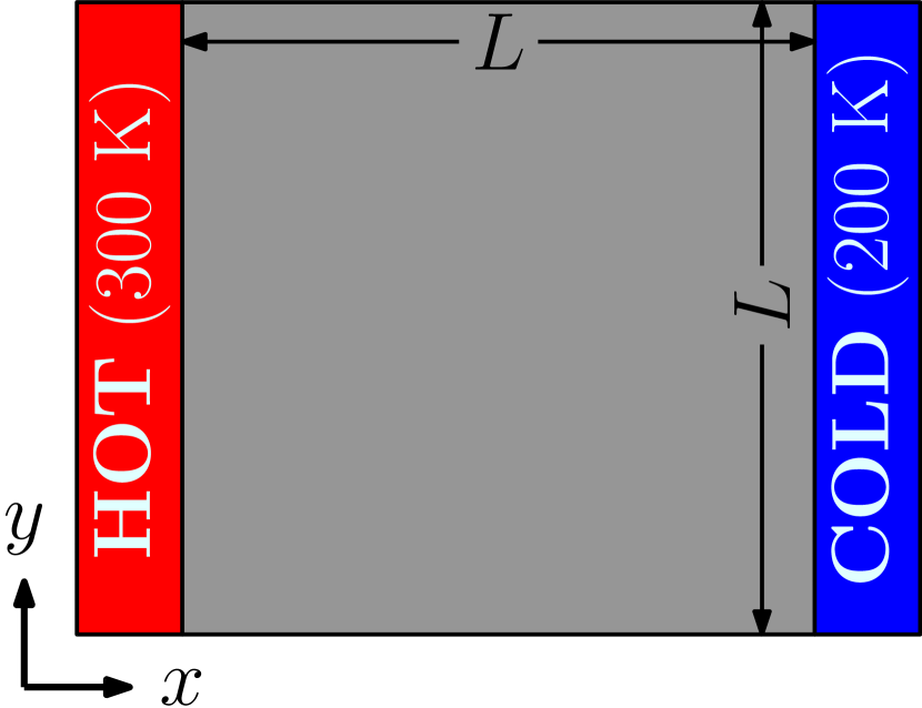
(a) A base material plate under constant heat flux.

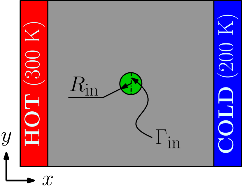
(b) An obstacle embedded in the plate.

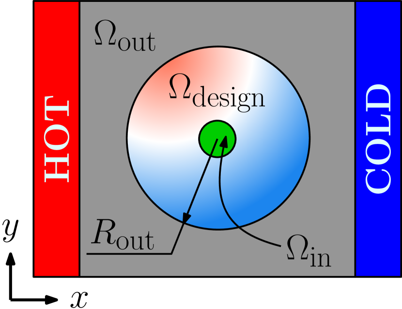
(c) A FGM-based cloak in the base material plate.

Figure 4: Schematic design of (a) a base material plate under constant heat flux applied by the high-temperature source on the left side and low-temperature sink on the right side; (b) a circular insulator embedded in the base material plate ($\mathrm{\Omega}_{\mathrm{in}}$ is the insulator); (c) the insulator and a surrounding FGM-based thermal cloak embedded in the base material plate; $\mathrm{\Omega}_{\mathrm{design}}$ is the domain of the cloak where the material distribution is optimized, $\mathrm{\Omega}_{\mathrm{out}}$ is the outside domain of remaining base material, where the temperature disturbance reduction is sought. $\mathrm{\Omega}=\mathrm{\Omega}_{\mathrm{in}}\cup\mathrm{\Omega}_{\mathrm{design}}\cup\mathrm{\Omega}_{\mathrm{out}}$.

We begin by designing 2D thermal cloaks, for which we consider an $L$ $\times$ $L$ square homogeneous base material plate. The plate is embedded by a circular insulator (with conductivity $\kappa_{\rm ins}=0.0001$ W/mK) of radius $R_{\rm in}$. Later, surrounding the insulator, an annular-shaped FGM-based thermal cloak with inner radius $R_{\rm in}$ and outer radius $R_{\rm out}$ is also added. Similar to the explanation in Section 2.1, by introduction of the insulator and thermal cloak, the plate domain $\Omega$ is divided into three parts: $\mathrm{\Omega}_{\rm in}$, $\mathrm{\Omega}_{\rm design}$ and $\mathrm{\Omega}_{\rm out}$ that possess the material properties of the insulator, FGM and base material, respectively. Constant temperatures, 300 K on the left side and 200 K on the right side are applied. Adiabatic wall condition is imposed on the top and bottom edges. The schematics related to the geometry are given in Figure 4. This geometry will be consistently utilized in several of the examples throughout this article, potentially with different dimensions and/or material allocations. In this particular case, we take $L=140$ mm, $R_{\rm in}=10$ mm, $R_{\rm out}=50$ mm, and iron as the base material ($\kappa_{\rm base}=67$ W/mK).

The objective of a thermal cloak is to reduce the temperature disturbance in the outer region $\Omega_{\rm out}$ caused by the presence of an insulator. In that manner, a thermal cloak ensures that the insulator does not get detected in the two points/four points in-plane observation of the temperature profile. Keeping this in mind, we define the cloaking objective function as:

$$J_{\mathrm{cloak}}=\dfrac{1}{\widetilde{J}_{\mathrm{cloak}}}\int_{\mathrm{\Omega}_{\mathrm{out}}}(T-\overline{T})^{2}~d\mathrm{\Omega},\quad\text{with}\quad\widetilde{J}_{\mathrm{cloak}}=\int_{\mathrm{\Omega}_{\mathrm{out}}}(\widetilde{T}-\overline{T})^{2}~d\mathrm{\Omega}.$$ (31)

where $\overline{T}$ is the temperature distribution of the reference case (a homogeneous base material plate without the presence of the insulator and thermal cloak), $\widetilde{T}$ is the temperature distribution when $\mathrm{\Omega}_{\rm design}$ is filled with the base material.

For NURBS parameterizations, the circumferential direction and radial direction are taken as the parametric directions. Also, second-order and first-order NURBS approximations are taken in circumferential direction and radial direction, respectively. A mesh model of a 2D NURBS patch is shown in Figure 1. Most of the 2D thermal cloaks have symmetry (adiabatic symmetry) along $x$ and anti-symmetry (isothermal symmetry) along $y$-axes. Thus, we impose $x$ and $y$-axes symmetry for the design meshes to reduce the corresponding number of design variables. Following it, we perform a mesh sensitivity analysis to choose an appropriate solution mesh as presented in B. Accordingly, we take a mesh with DOF=13167 as the solution mesh for $N_{\rm var}=25$ and $N_{\rm var}=81$.

5.1.1 Design with various material models

EMT
$v_{i}\in[0,1]$	Maxwell
$v_{i}\in[0,1]$	Porous Cu
$v_{i}\in[0,0.7]$	Cu-Sn-Pb
$v_{i}\in[0,0.3]$	TCOH
${v_{i}\in[0.2,0.8]}$	Gyroid
$v_{i}\in[0.2,0.9]$
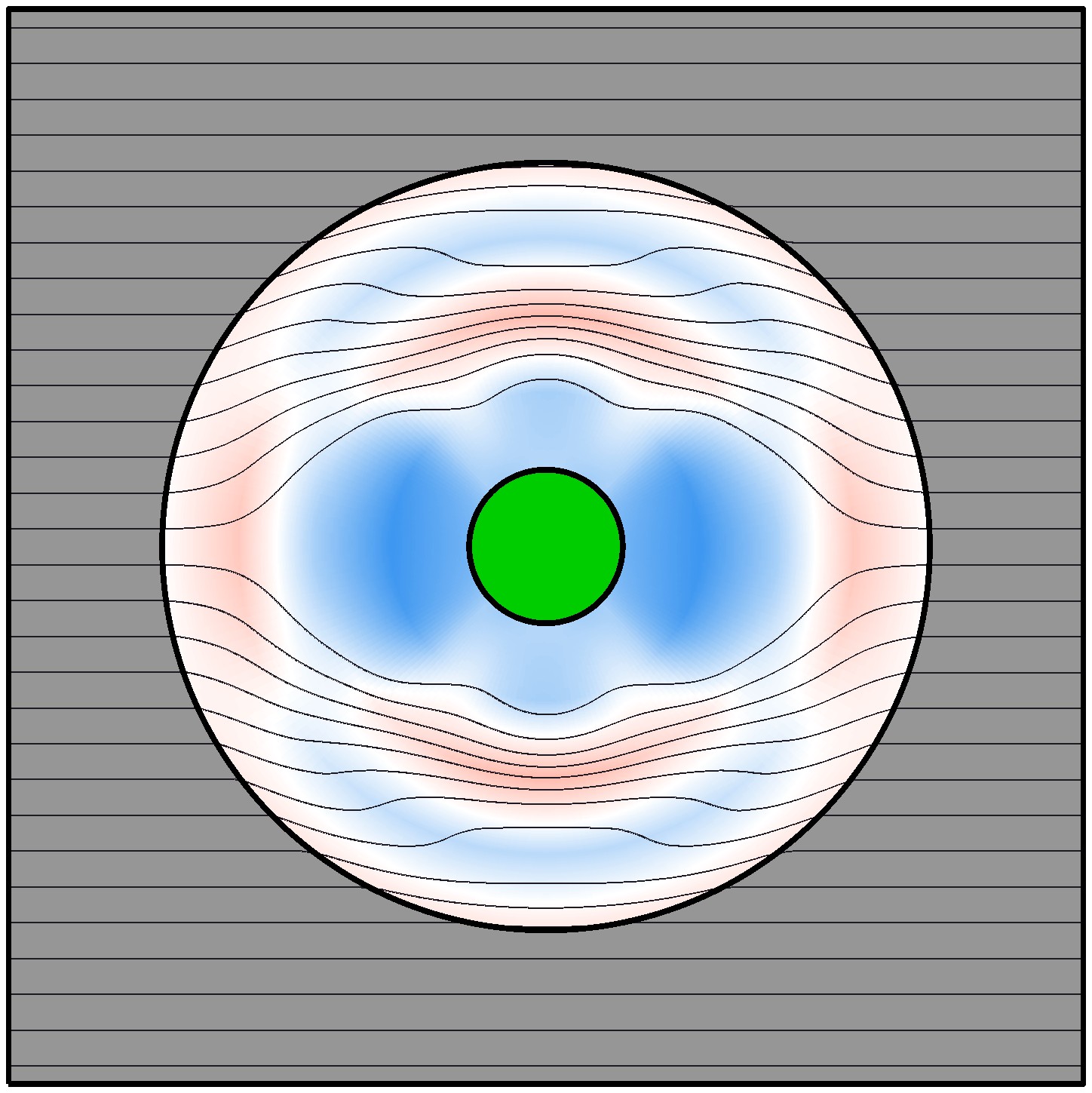
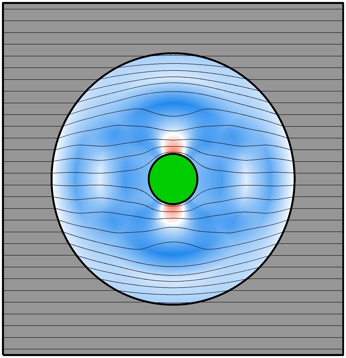
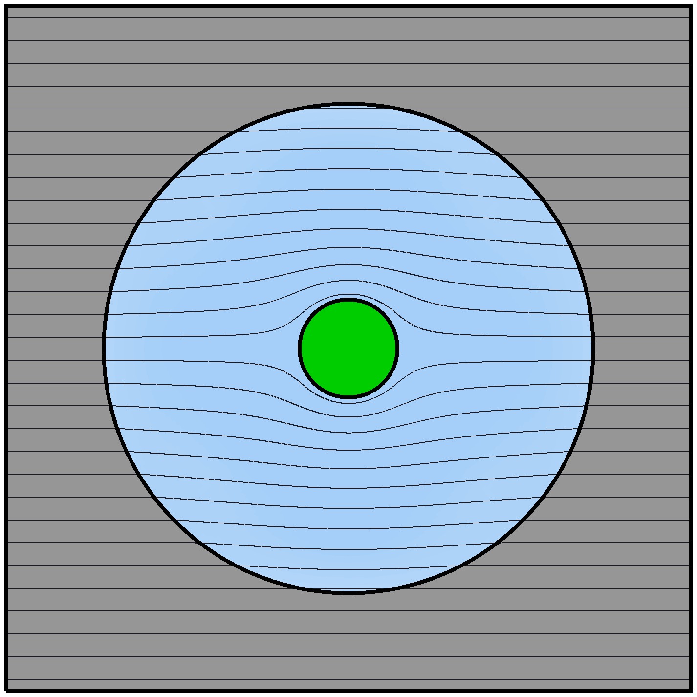
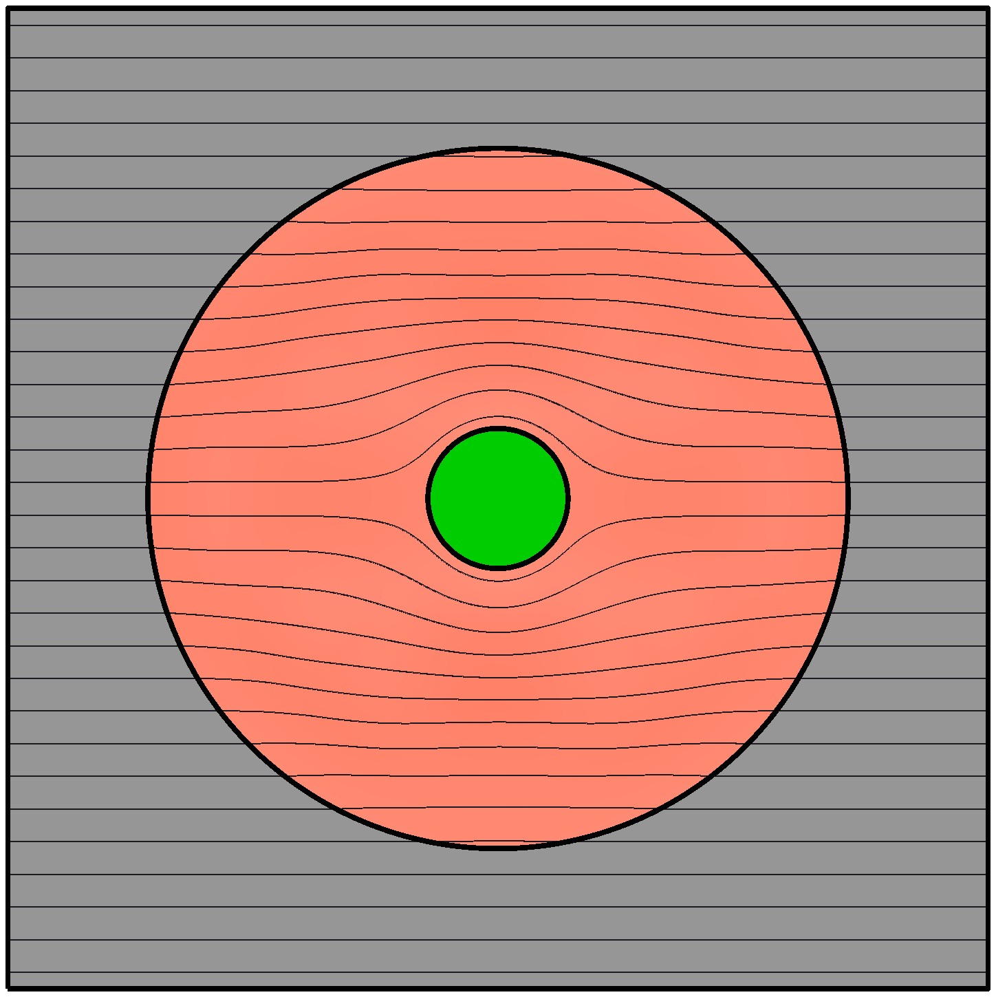
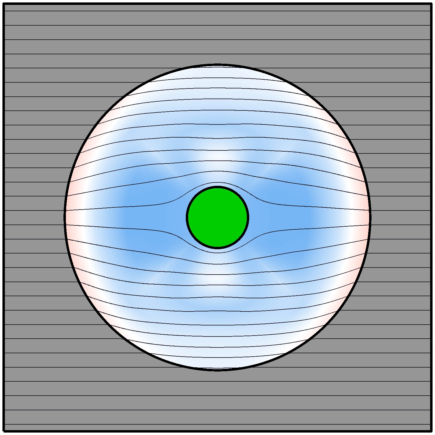
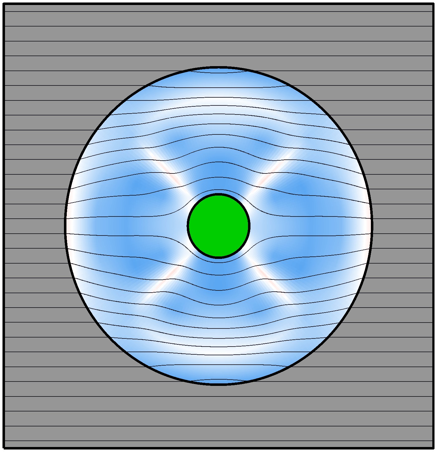
(a) $N_{\rm var}=25$, $J=8.74\times 10^{-9}$	(b) $N_{\rm var}=25$, $J=9.91\times 10^{-9}$	(c) $N_{\rm var}=25$, $J=2.01\times 10^{-8}$	(d) $N_{\rm var}=25$, $J=1.94\times 10^{-8}$	(e) $N_{\rm var}=25$, $J=1.21\times 10^{-7}$	(f) $N_{\rm var}=25$, $J=7.55\times 10^{-8}$

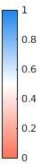
Figure 5: Optimized material distributions for the thermal cloak problem. Six material models and $N_{\rm var}=25$ are considered. Optimized objective function values are of order $10^{-7}$-$10^{-9}$. In optimized material distributions, almost the entire design domain filled with intermediate densities.

In Figure 5.1.1, we show the optimized material distributions for thermal cloak using 6 different effective thermal conductivity models (given in Table 1) for $N_{\rm var}=25$. As the solution of the thermal cloak problem is non-unique [65, 66, 67] and most topology optimization problems are non-convex, our optimization cases reach the nearest local minimizers. Therefore, as depicted in the figure, the optimized material distributions remain close to the initial material distributions with almost the entire domain filled with intermediate densities. All these distributions are valid solutions and exhibit objective function value of order $10^{-7}$-$10^{-9}$.

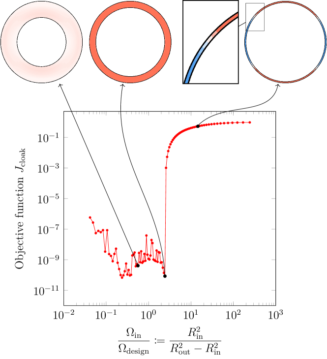
Figure 6: Trend of the objective function $J_{\rm cloak}$ vs. $\Omega_{\rm in}/\Omega_{\rm design}$. $R_{\rm in}$ is varied between $10$ mm to 49 mm, while keeping $R_{\rm out}=50$ mm constant. For $R_{\rm in}\lessapprox 42.2$ mm, the designed cloaks have satisfactory cloaking function with $J_{\rm cloak}<10^{-6}$. As the insulator size increases more than 42.2 mm, $J_{\rm cloak}$ increases exponentially.

Next, we want to study the effect of design domain size with respect to the insulator size on the overall optimization results. Therefore, we run optimization with different values of $R_{\rm in}$ (between $10$ mm and 50 mm) while keeping $R_{\rm out}=50$ mm constant. The plot of $J_{\rm cloak}$ vs ${\Omega_{\rm in}}/{\Omega_{\rm design}}$ for $N_{\rm var}=25$ and EMT model is presented in Figure 6. From the figure, it is evident that the proposed method is capable of designing thermal cloaks of substantial quality for $R_{\rm in}\lessapprox 42.2$ mm (or ${\Omega_{\rm in}}/{\Omega_{\rm design}}\lessapprox 2.48$) with $J_{\rm cloak}<6\times 10^{-7}$. At $R_{\rm in}\approx 42.2$ mm, the optimized material distribution completely filled $\Omega_{\rm design}$ with copper. This optimized material distribution aligns with the concept of a bilayer cloak, as proposed by Han et al. [8] and verified in our previous study [24]. A bilayer cloak consists of two annular layers: an outer layer made of a material with higher conductivity and an inner layer composed of an insulating material. The radius of the circular interface between these layers is uniquely determined by the conductivities of the materials involved. In our scenario, this interface radius would be $R_{\rm out}\sqrt{(\kappa_{\rm copper}-\kappa_{\rm base})/(\kappa_{\rm copper}+\kappa_{\rm base})}$= 42.18 mm. Thus, we can say that $R_{\rm in}\lessapprox 42.18$ mm represents a bilayer cloak without an inner layer. This also shows the minimum required design domain to attain a significant cloaking effect based on the given conductivities. Reducing the design domain below this threshold limits the available design space, consequently deteriorating optimization scope severely. Therefore, as $R_{\rm in}$ becomes greater than $42.2$ mm, $J_{\rm cloak}$ starts rising exponentially to approach 1.

To showcase the cloaking performance of optimized cloaks, we present the flux flow, temperature profile and temperature difference with respect to a homogeneous base material plate in Figure 7. We exhibit the thermal cloaks obtained using EMT and Cu-Sn-Pb models for $N_{\rm var}=25$ and $R_{\rm in}=35$ mm. Here, we use a larger insulator to highlight the cloaking effect. We can witness substantial thermal cloaking in $\Omega_{\rm out}$, characterized by minimal temperature disruption, even within a temperature range that is 3-4 orders of magnitude smaller than the actual temperature range.

	A square homogeneous base material plate	A square base material plate embedded by a circular insulator ($J=1$)	A square base material plate embedded by a circular insulator and surrounding thermal cloak
			EMT ($J=1.97\times 10^{-9}$)	Cu-Sn-Pb ($J=4.32\times 10^{-9}$)
Flux flow
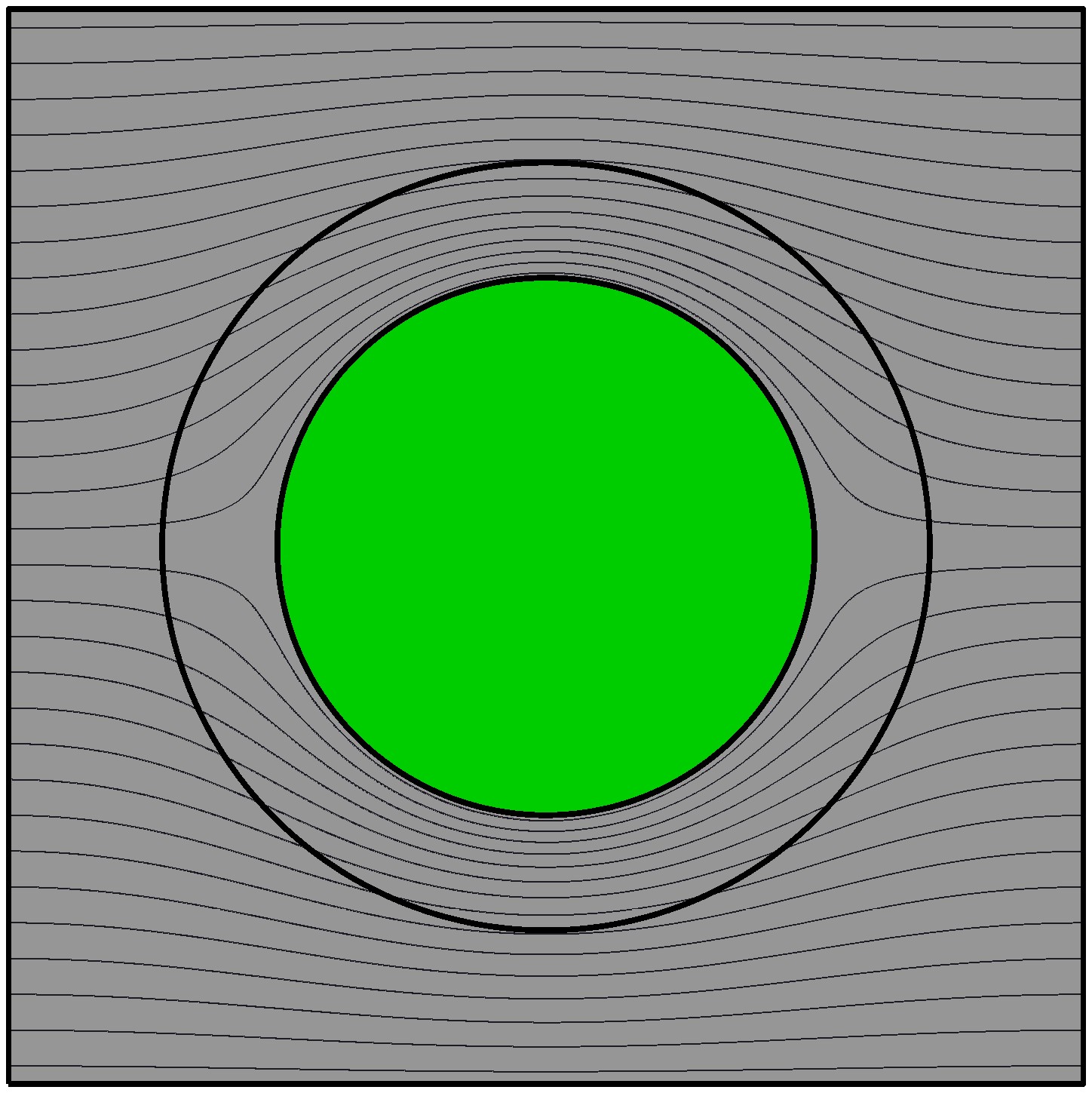
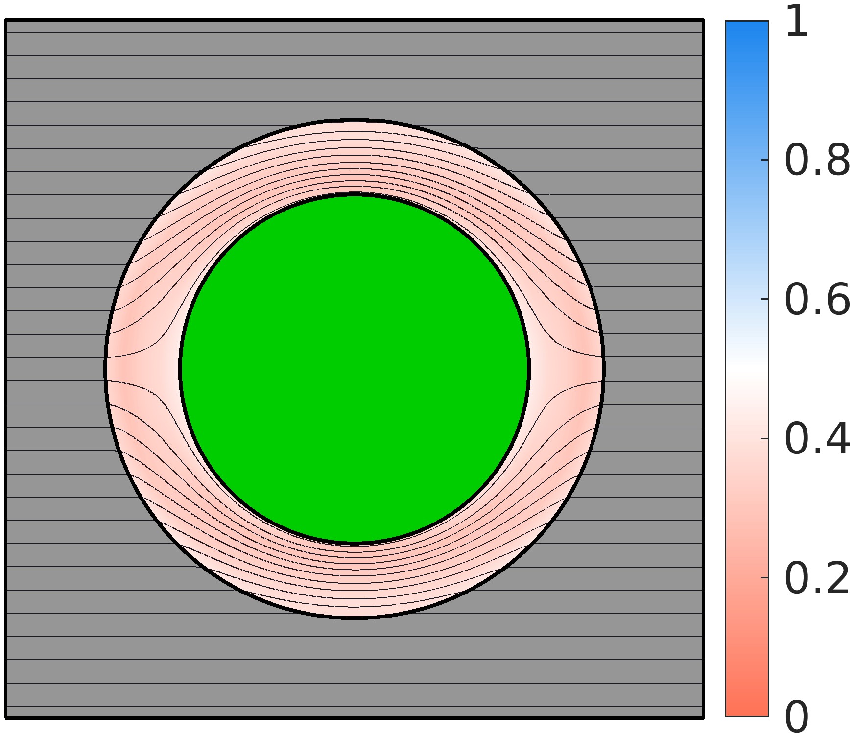
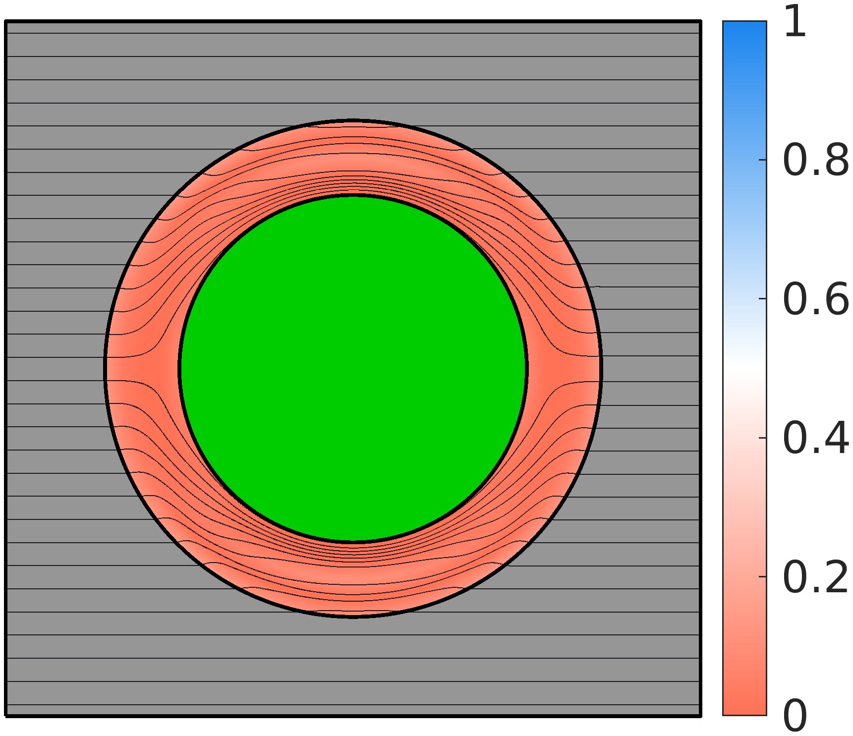
Temp. $T$
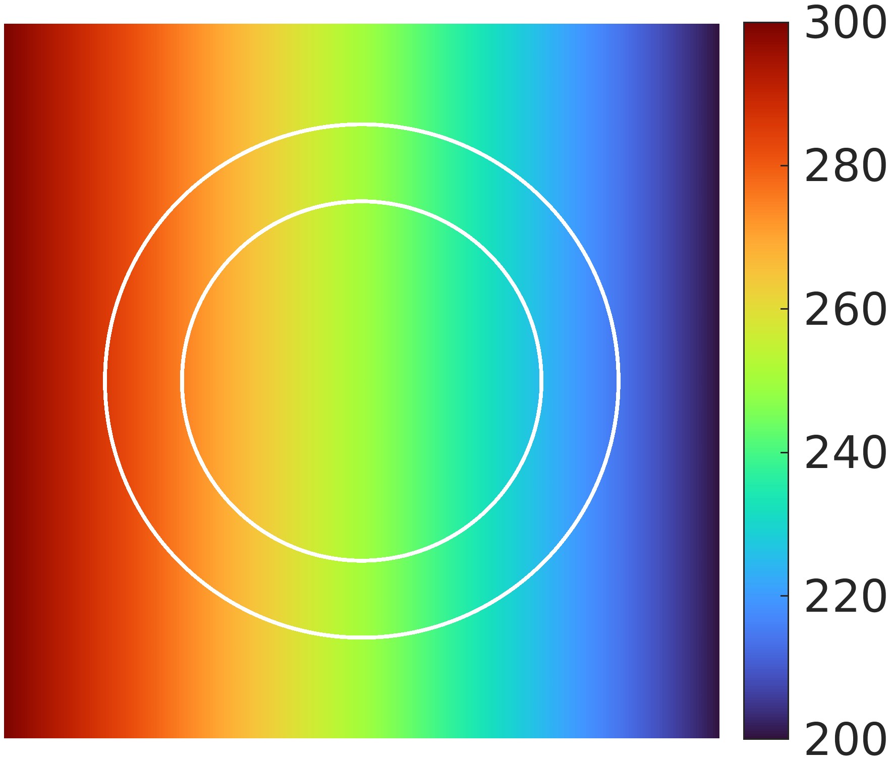
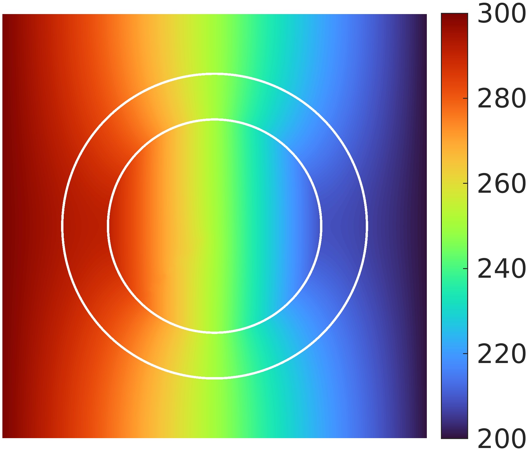
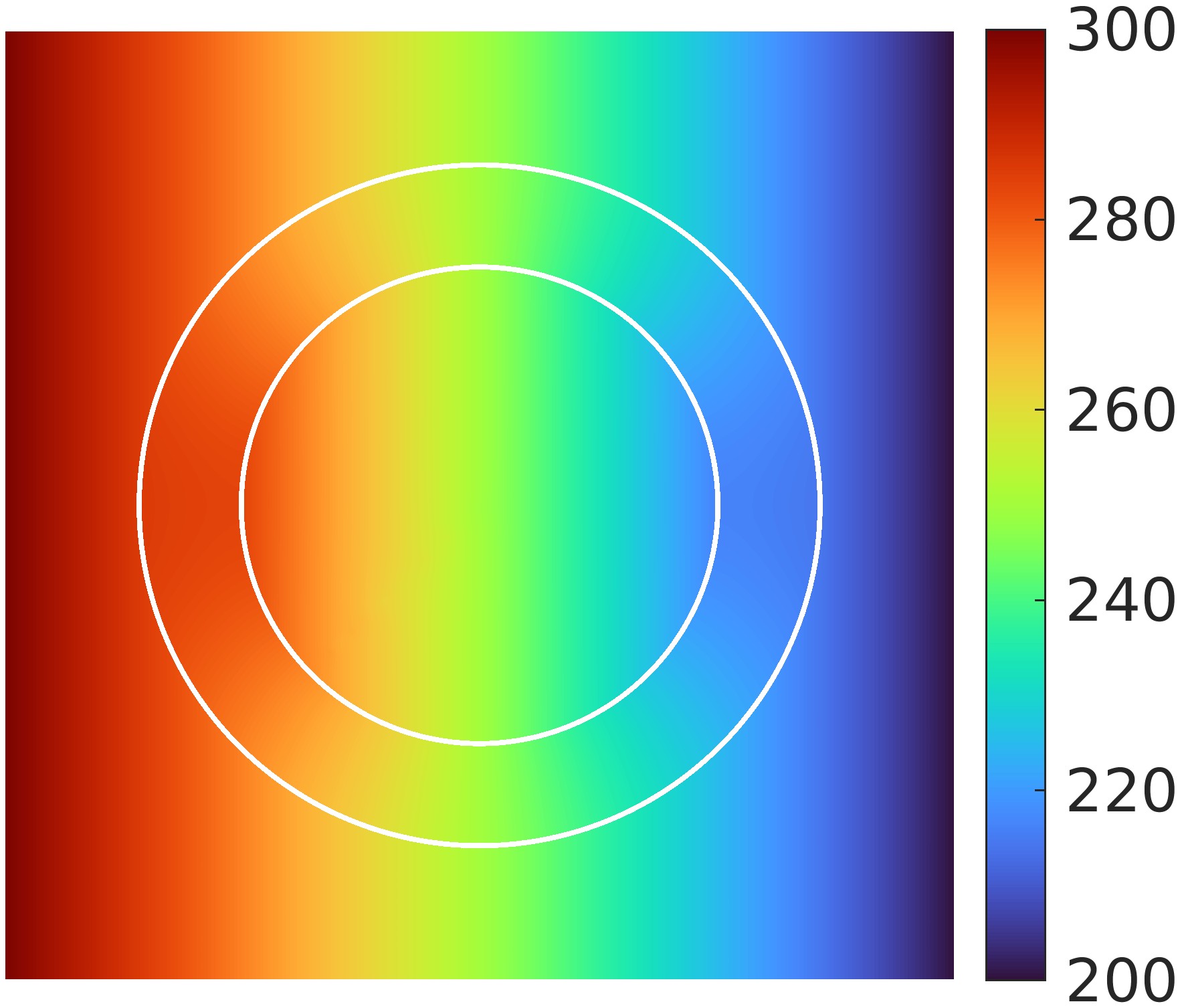
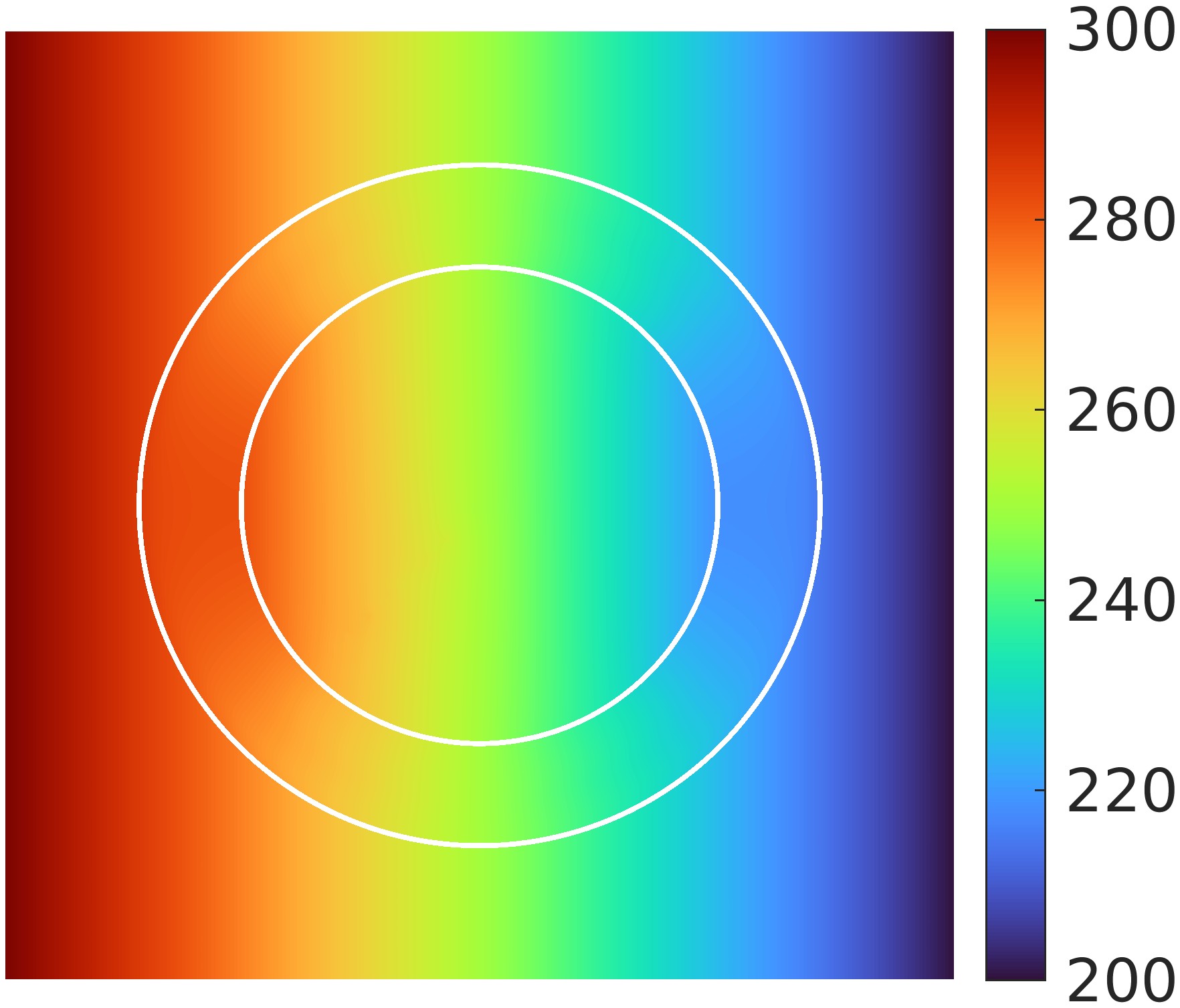
Temp. Diff. $T-\overline{T}$

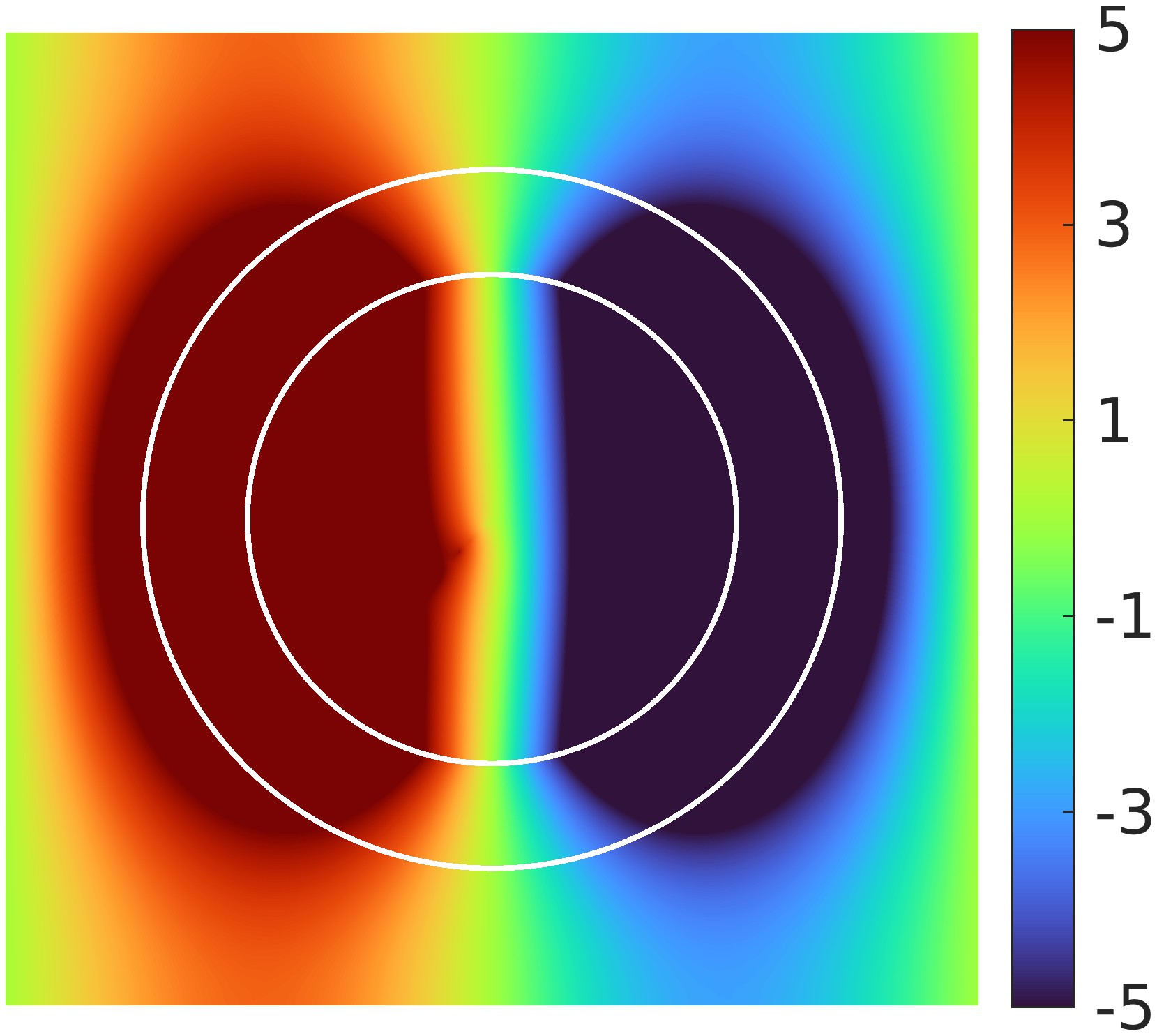
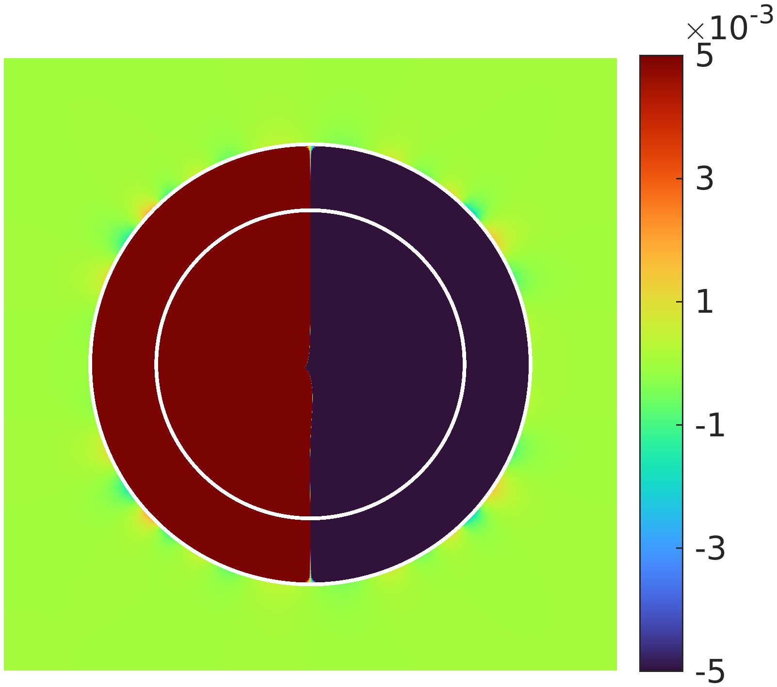
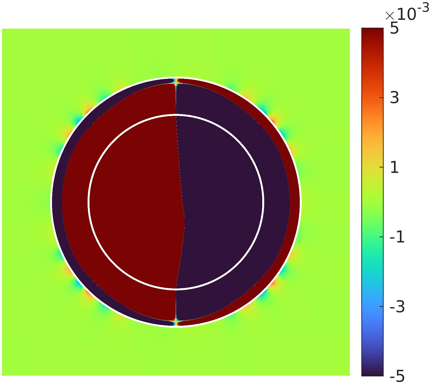
Figure 7: Flux flow and temperature distribution $T$ for (first column) a homogeneous base material plate (reference case), (second column) a base material plate embedded with a circular insulator, and (third & forth column) a base material plate embedded with a circular insulator and surrounding thermal cloak (optimized using EMT and Cu-Sn-Pb material models, $R_{\rm in}=35$ mm and $N_{\rm var}=25$). Temperature differences with respect to the reference case $T-\overline{T}$ are also presented. The thermal cloaks effectively diminish the temperature disturbance in $\mathrm{\Omega}_{\mathrm{out}}$. Temperature disturbances are almost nul in $\mathrm{\Omega}_{\mathrm{out}}$, even with the 3-4 order smaller temperature range.

As mentioned in the introduction, the thermal cloak problem falls under the Calderón tomography problem [65, 66], which has multiple solutions [67]. Due to this non-uniqueness, the optimization results are mesh as well as initial point-dependent. We tested five different values of $v_{i}$, $i=1,2,...,N_{\rm var}$; $v_{i}=$ 0, 0.25, 0.5, 0.75, 1 for initial distributions for $N_{\rm var}=25$, $R_{\rm in}=10$ mm and EMT model. In Figure 8, the optimization results clearly display the dependency on the initial distribution. This lack of well-posedness of the problem can be mitigated (but not avoided) by imposing regularizations/constraints.

$v_{i}=0$	$v_{i}=0.25$	$v_{i}=0.5$	$v_{i}=0.75$	$v_{i}=1$
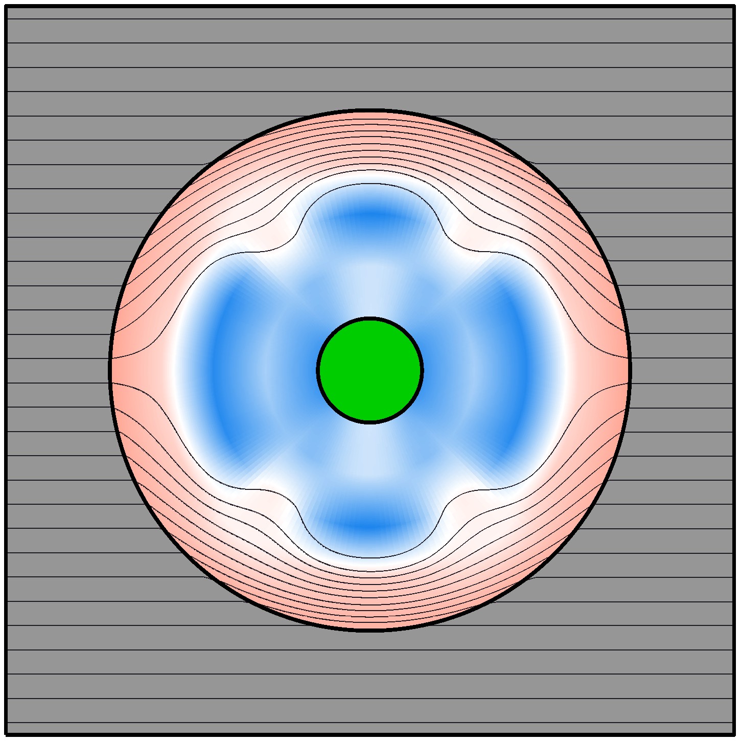
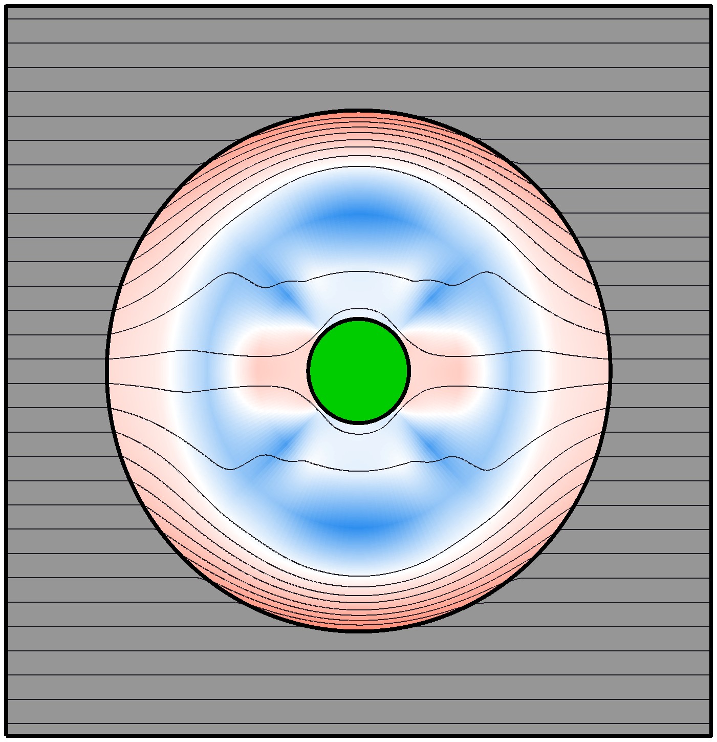
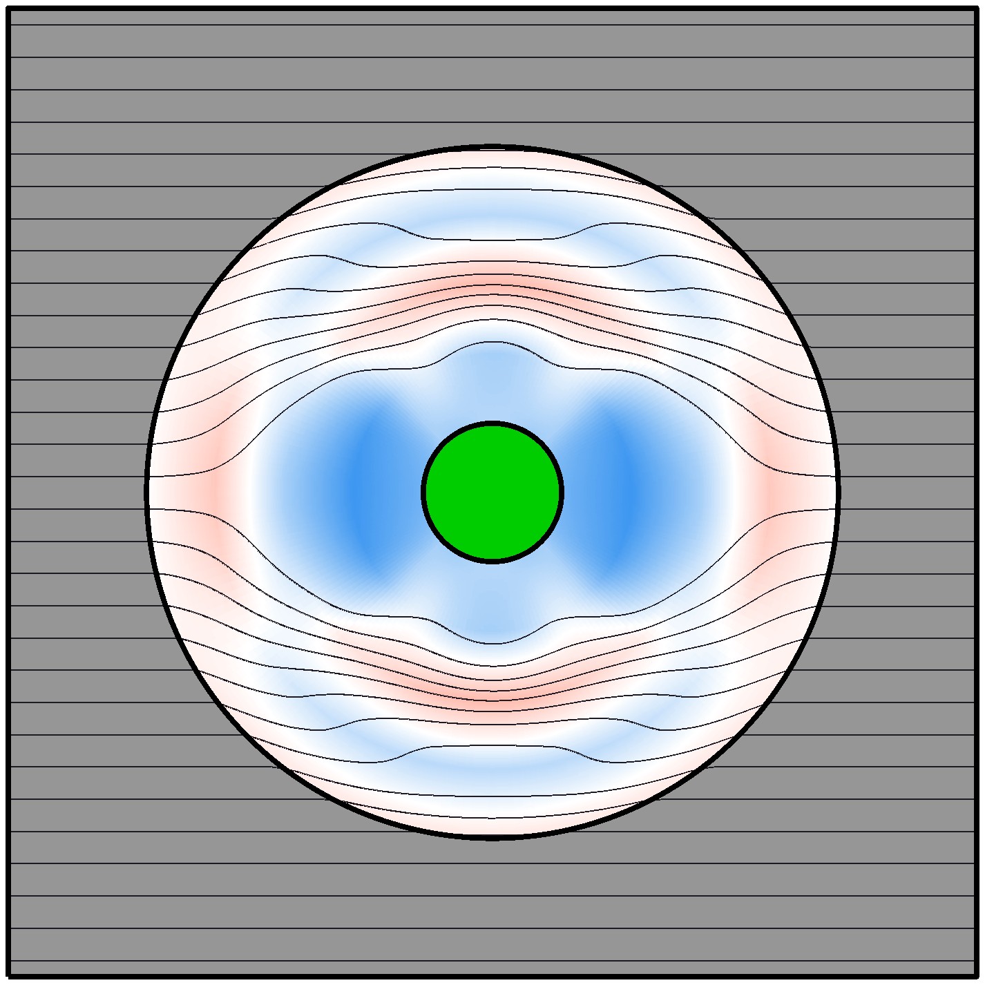
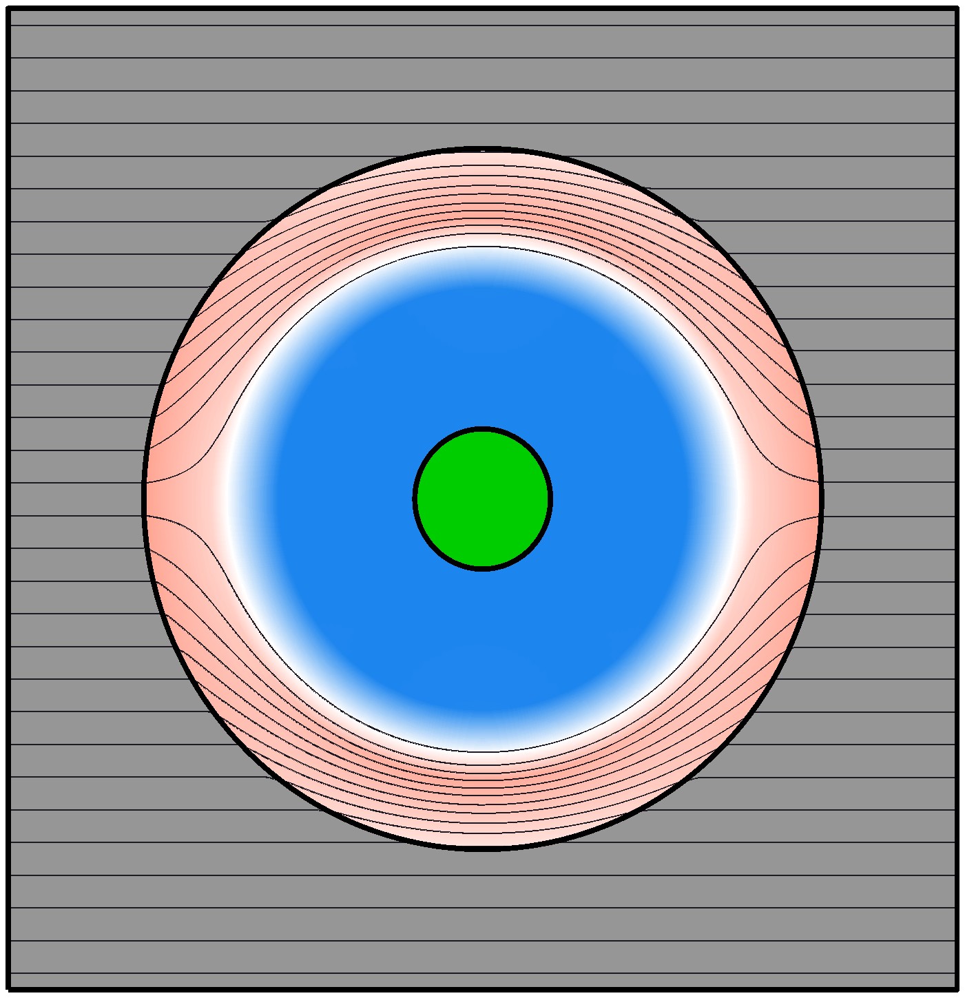
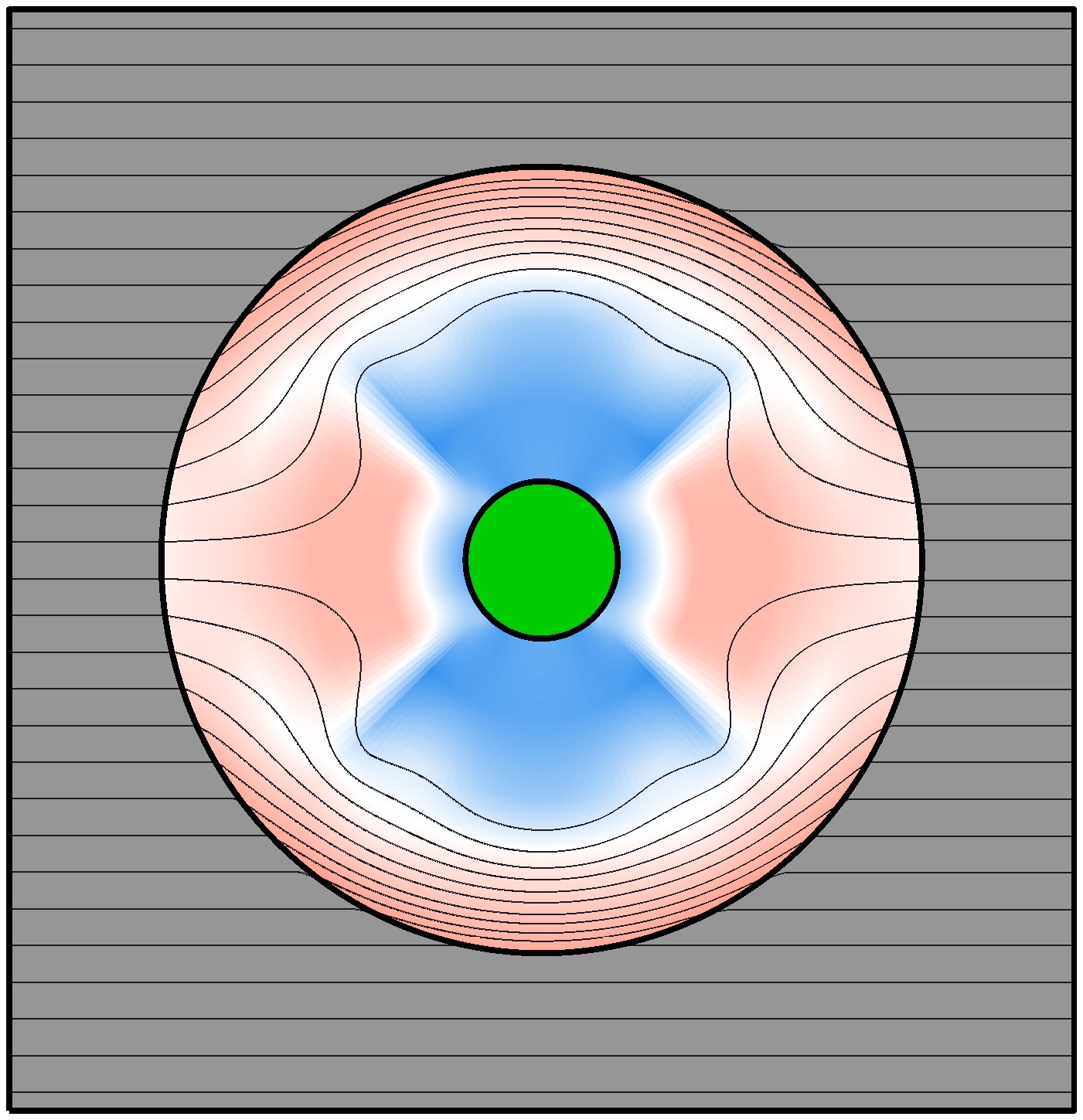
(a) $N_{\rm var}=25$, $J=3.76\times 10^{-8}$	(b) $N_{\rm var}=25$, $J=8.47\times 10^{-8}$	(c) $N_{\rm var}=25$, $J=8.74\times 10^{-9}$	(d) $N_{\rm var}=25$, $J=5.55\times 10^{-8}$	(e) $N_{\rm var}=25$, $J=1.60\times 10^{-7}$

Figure 8: Optimized material distributions for the thermal cloak problem with five different initial relative density distributions, $v_{i}=0,0.25,0.5,0.75,1$, $i=1,2,...,N_{\rm var}$. EMT material model and $N_{\rm var}=25$ is considered. Optimized objective function values are of order $10^{-9}$-$10^{-11}$. Optimization results are dependent on the initial relative density distribution.

5.1.2 Design with constraints

A major limitation of conventional analytical methods is their inability to deal with free-form shapes, boundary conditions and design restrictions. This is one of the reasons why most thermal cloaks in the literature are designed for limited regular shapes (like circular [10, 8] and elliptical shapes [94]) and simple boundary conditions without any design constraints [10, 8, 9, 95, 96]. In the next few subsections, we explore the application of the proposed method to overcome above-mentioned limitations of the conventional methods.

In order to make practical designs, the optimization often needs to follow design, manufacturing or material restrictions. This subsection focuses on the application of such restrictions on the thermal cloak design problem. We explore two schemes to apply restrictions, one via adding a regularization/penalty term in the primary objective function and another via including a constraint in the optimization problem.

First, we consider the design requirement to have a large area covered by pure materials and only the most crucial areas occupied by the intermediate densities. To include this requirement, the objective function is augmented by an extra penalty term $J_{\rm Intpen}$ using the weight factor $\chi$. The penalty term $J_{\rm Intpen}$ penalizes the intermediate densities. The final objective function and the penalty term are presented as follows:

$$J=J_{\rm cloak}+\chi J_{\mathrm{Intpen}}\quad\text{with}\quad J_{\rm Intpen}=\int_{\Omega_{\rm design}}v^{4}(1-v)^{4}~d\Omega.$$ (32)

By the weighting factor $\chi$, we delay the impact of the penalty term to secure a sufficient value of the primary objective function before the effect of penalization starts. Also, as mentioned in Section 4.1, finding the derivative of $J_{\rm Intpen}$ with respect to design variables will be straightforward using Eq. (8), owing to the NURBS parameterization for the density field.

w/o reg.	$\chi=0.01$	$\chi=1$	$\chi=100$
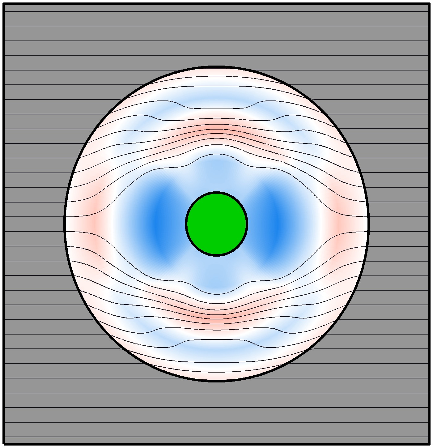
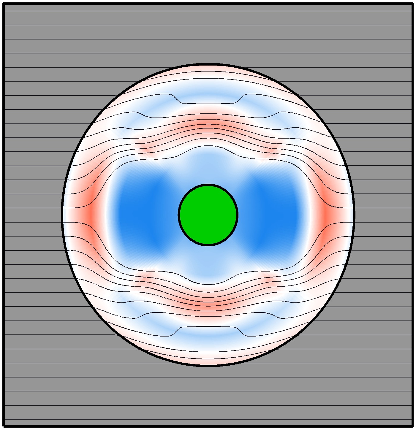
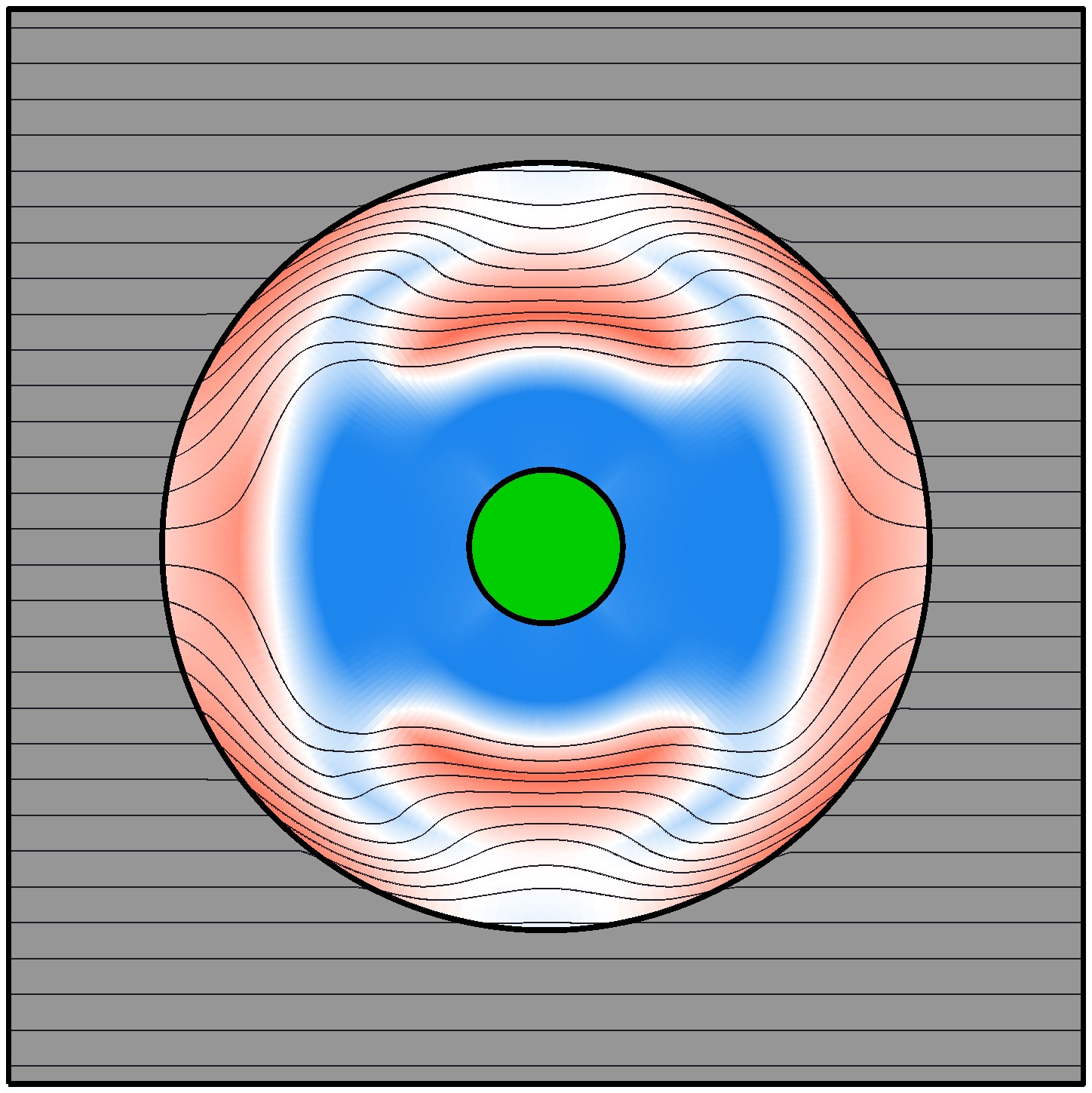
(a) $J=7.35\times 10^{-11}$, $J_{\rm cloak}=7.35\times 10^{-11}$.	(b) $J=2.94\times 10^{-7}$, $J_{\rm cloak}=6.05\times 10^{-8}$, $J_{\rm Intpen}=2.33\times 10^{-7}$.	(c) $J=1.97\times 10^{-5}$, $J_{\rm cloak}=2.56\times 10^{-7}$, $J_{\rm Intpen}=1.95\times 10^{-5}$.	(d) $J=1.24\times 10^{-3}$, $J_{\rm cloak}=1.27\times 10^{-5}$, $J_{\rm Intpen}=1.23\times 10^{-3}$.

Figure 9: (Columns 2-4) Optimized material distributions for the thermal cloak problem with the intermediate density penalization. EMT material model and $N_{\rm var}=25$ are considered. Three values of $\chi$, $\chi=~0.01$, $0.1$, $1$, are tested. Optimized objective function value are of order $10^{-4}-10^{-5}$ with $J_{\rm cloak}$ of order $10^{-7}$ and $J_{\rm Intpen}$ of order $10^{-4}-10^{-5}$. The left column represents the optimized material distribution of the cloak without penalization. The penalization effectively reduces the area with intermediate densities with a slight compromise in the main cloaking objective.

In Figure 9, we have shown the results with penalization for the EMT model with $N_{\rm var}=25$. We consider three values of $\chi$, $\chi=10^{-2}$, $1$ and $100$. We can see that, by increasing the value of $\chi$, the optimized results move towards the material distributions with large areas of pure constituent materials. The penalization comes with a slight compromise in the main cloaking objective. Yet, all designs shown in Figure 9 reach $J_{\rm cloak}$-value in the range of $10^{-5}$, showcasing satisfactory cloaking function. With a very large value of $\chi$, the method produces almost binary 0-1 type designs. This behaviour is similar to the SIMP interpolation scheme. The distinction, however, lies in the penalization, which comes from the extra objective function term in contrast to the material law as in the SIMP. A prediction of an appropriate value of $\chi$ is very difficult apriori and needs a trial-and-error study. Another point worth mentioning is one can use any power to the density terms in the definition of $J_{\rm Intpen}$. The power will regulate how sharply the effect of penalization changes with $\chi$.

Secondly, we consider a localized maximum temperature constraint in the optimization problem. This constraint can be included when there is a requirement to maintain a specific maximum temperature in a local region of the domain. This requirement could attributed to the material or working environment limitations. To apply the maximum temperature numerically, we need a formula to approximate the maximum temperature, $\tau_{\rm max}$. Here, we exploit the approximation utilized in [97, 98] in a continuum framework, and the corresponding constraint is defined as:

$$\tau_{\rm max}(\varphi)\leq T_{\rm max}\quad\text{with}\quad\tau_{\rm max}=\dfrac{\int_{\Omega}TA^{T}H(\varphi)~d\Omega}{\int_{\Omega}A^{T}H(\varphi)~d\Omega},$$ (33)

where $T_{\rm max}$ is the upper limit of the permissible temperature, $A$ is the constant that makes $\tau_{\rm max}$ the maximum approximate temperature as $A^{T}\rightarrow+\infty$ (In this example, we take $A=1.5$), $\varphi$ is the signed function to represent the temperature constrained region and $H(\varphi)$ is the Heaviside function.

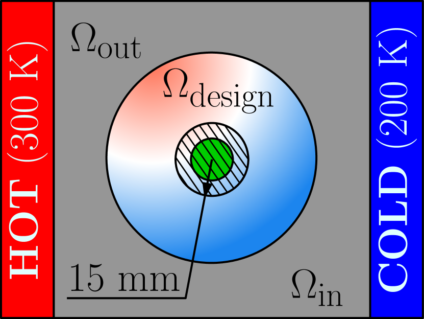
(a) Problem domain

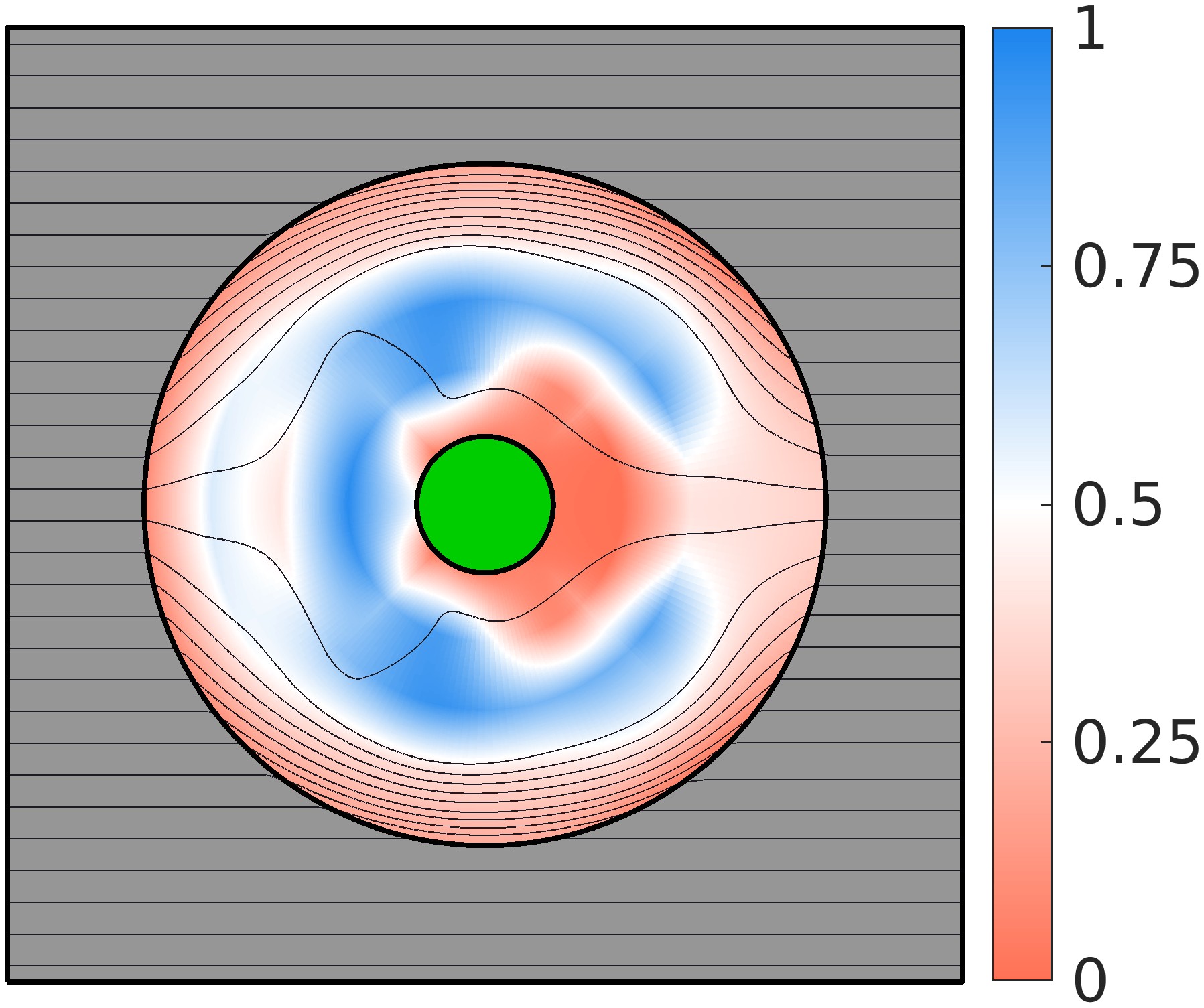
(b) Optimized material distribution

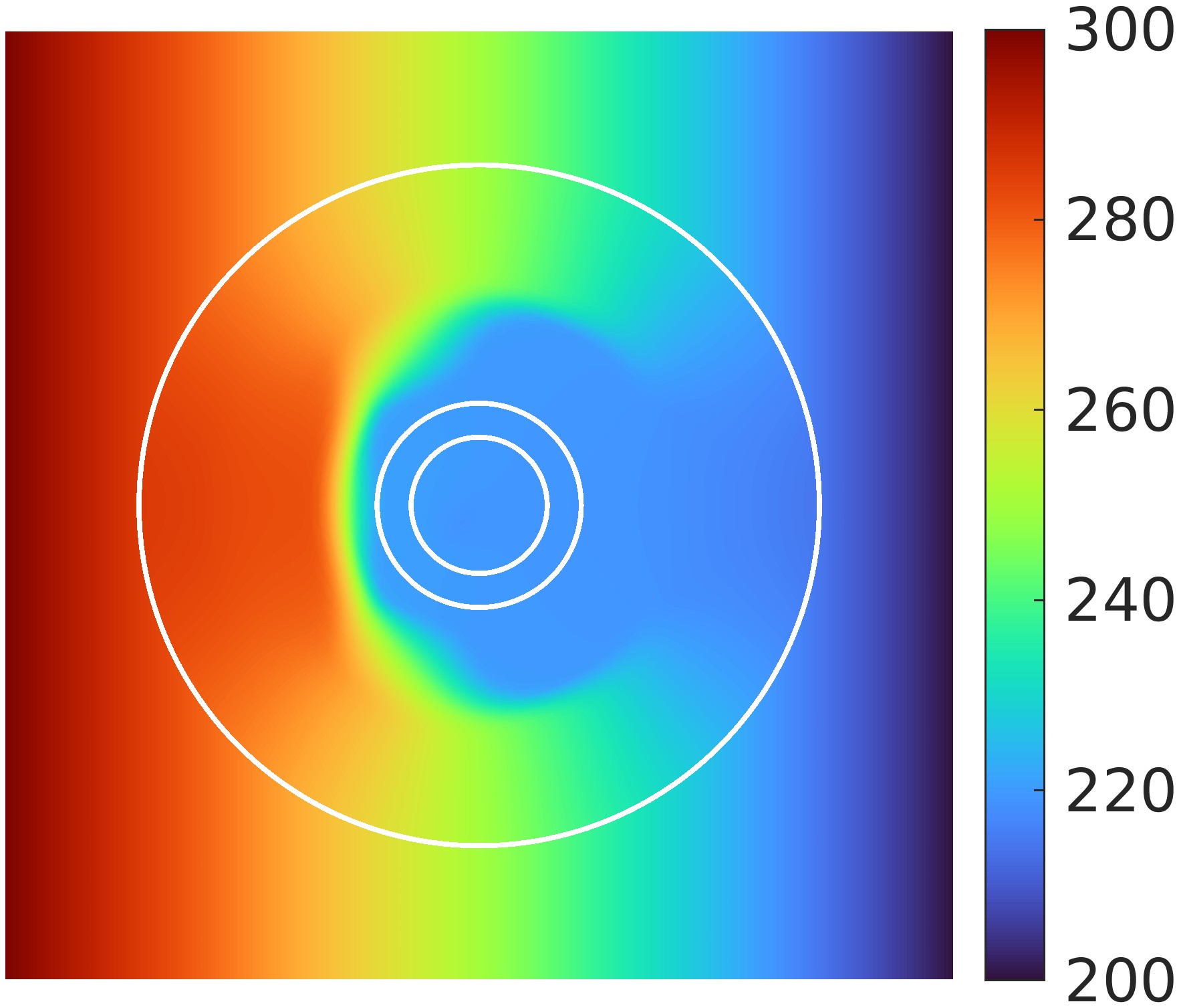
(c) Temperature $T$ distribution

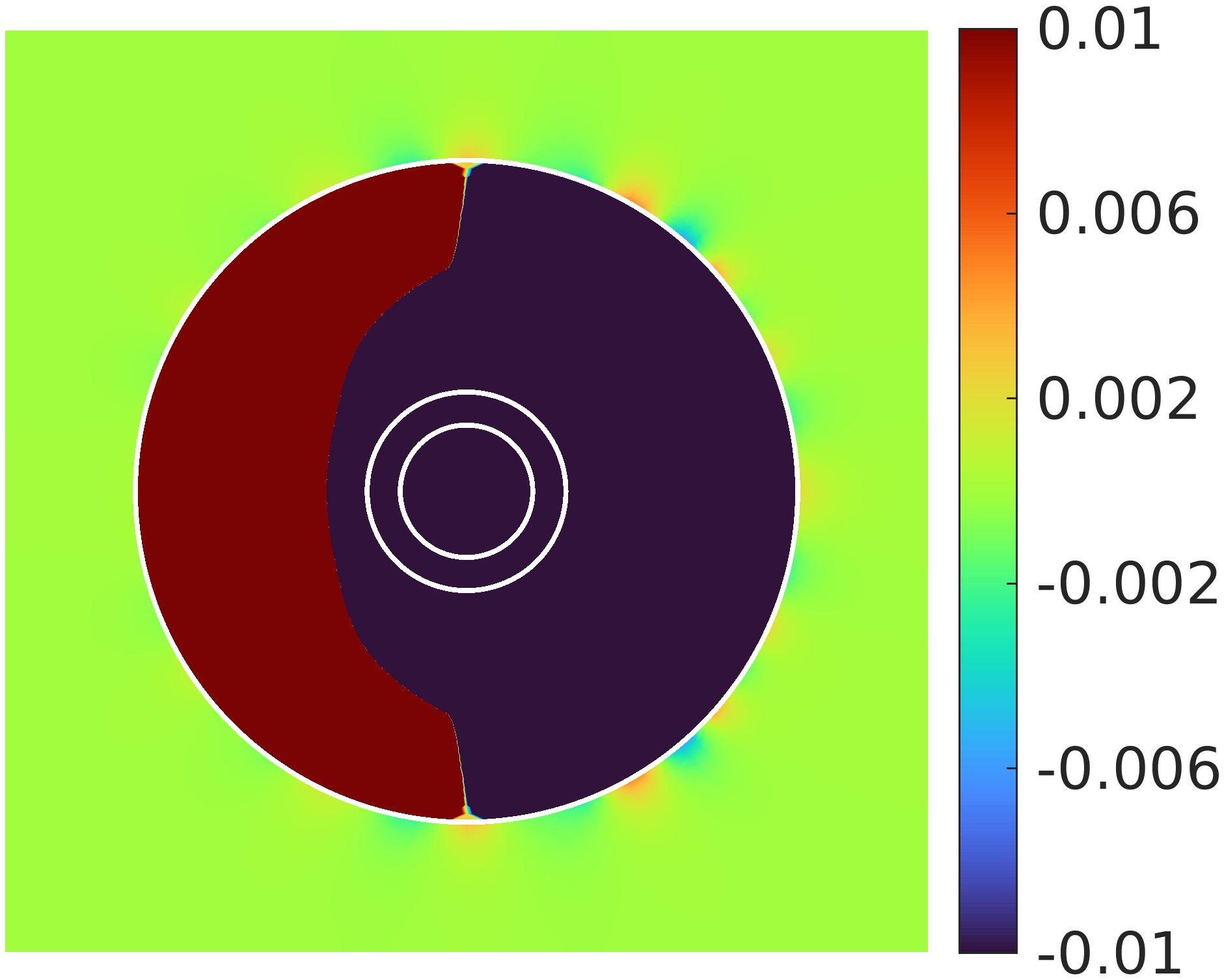
(d) Temp difference $T-\overline{T}$

Figure 10: Problem domain, optimized material distribution, temperature $T$ distribution and temperature difference (with respect to the reference case) $T-\overline{T}$ for the thermal cloak problem with a localized maximum temperature constraint. EMT material model, $N_{\rm var}=50$ and $T_{\rm max}=220$ K are considered. The hatched area presents the region where the constraint is applied. Optimized material distribution maintains the temperature in the hatched area below $T_{\rm max}=220$ K while cloaking the insulator with the objective function value $J=1.68\times 10^{-6}$.

For our design problem, we want to keep the temperature in a circular region with radius 15 mm at the center (covering the insulator and a small surrounding region) lower than or equal to $T_{\rm max}=220$ K. The local region under constraint is shown as the hatched area in Figure 10(a). The optimization problem with the constraint is not symmetric along $y$-axis, therefore we remove the symmetry condition along $y$-axis for the design variables. In order to solve the optimization problem, the optimization algorithm also necessitates the sensitivities of the constraint function with respect to the design variables. To calculate these constraint sensitivities, an extra adjoint problem is solved as presented in Eqs. (28)-(30) at each optimization iteration. The optimization results with the constraint for the EMT model with $N_{\rm var}=50$ are presented in Figures 10(b)-10(d). From the figure, we can observe that the temperature in the hatched region is lower than or equal to $T_{\rm max}$. Also, from Figure 10(d), it is evident that the satisfactory cloaking function is achieved with $J=1.68\times 10^{-6}$.

Both examples demonstrate how effortlessly the proposed method includes constraints in the formulation, which could be regarded as the primary benefit of the the proposed method from the manufacturing point of view. Though two specific types of constraints are presented in the subsection, the method is rather general and other constraints can be applied with equal effectiveness.

5.1.3 Design with free-form geometries

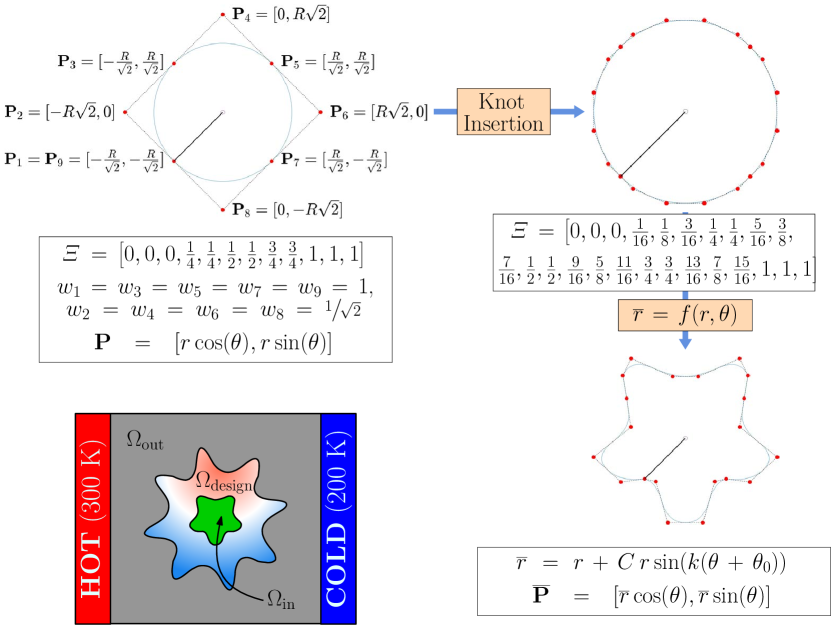
Figure 11: Steps to generate the star-shaped insulator & thermal cloak and schematics of the final domain. The control points related to the circumferential parametric directions of the circles of radius $R_{\rm in}$ and $R_{\rm out}$ are perturbed. The steps for perturbation are as follows: (i) A NURBS-circle is created using a knot vector $\Xi=[0,0,0,\nicefrac{{1}}{{4}},\nicefrac{{1}}{{4}},\nicefrac{{1}}{{2}},\nicefrac{{1}}{{2}},\nicefrac{{3}}{{4}},\nicefrac{{3}}{{4}},1,1,1]$ with nine control points $\mathbf{P}_{i}$, $i=1,2,...,9$. The Cartesian coordinates and weights of the control points are shown in the first figure. (ii) The NURBS-circle is refined by adding knots $\nicefrac{{1}}{{16}},\nicefrac{{1}}{{8}},\nicefrac{{3}}{{16}},\nicefrac{{5}}{{16}},\nicefrac{{3}}{{8}},\nicefrac{{7}}{{16}},\nicefrac{{9}}{{16}},\nicefrac{{5}}{{8}},\nicefrac{{11}}{{16}},\nicefrac{{13}}{{16}},\nicefrac{{7}}{{8}},\nicefrac{{15}}{{16}}$ through knot insertion procedure. (iii) The control points of the refined circle are transformed into polar coordinates $(r,\theta)$ from Cartesian coordinates $\mathbf{P}=(x,y)$; the radial coordinates $r$ are perturbed by the function, $\overline{r}=r+Cr\sin{(k(\theta+\theta_{0}))}$, while keeping $\theta$ coordinates unchanged; the modified polar coordinates $(\overline{r},\theta)$ are transformed back into Cartesian coordinates $\overline{\mathbf{P}}=(\overline{x},\overline{y})$. For $R_{\rm in}=15$ mm, $C=0.3$, $k=5$ and $\theta_{0}=\pi$, while for $R_{\rm out}=40$ mm, $C=0.4$, $k=8$ and $\theta_{0}=-\nicefrac{{\pi}}{{2}}$.

In this subsection, we study the effectiveness of our method for the star-shaped insulator and thermal cloak. To create both star-shaped geometries, we perturb the control points of NURBS-based circles of radius $R_{\rm in}$ and $R_{\rm out}$. For the perturbation, we perform knot insertion, coordinate-system transformations (from Cartesian to polar & from polar to Cartesian) and functional transformation of radial coordinates. The detailed procedure and the final domain are presented in Figure 11. For ${R_{\rm in}=15}$ mm, we use $C=0.3$, $k=5$ and $\theta_{0}=\pi$, while for $R_{\rm out}=40$ mm, we use $C=0.4$, $k=8$ and $\theta_{0}=\nicefrac{{-\pi}}{{2}}$. Other details are kept the same as the original cloak problem.

We consider three material models (EMT, Porous Cu and Gyroid) with ${N_{\rm var}=25}$. The optimized material distributions and temperature differences are shown in Figure 12. From the figure, we can see that the proposed method can effectively design the star-shaped thermal cloak around a free-form-shaped insulator without any issues. For EMT and Gyroid models, the optimization could achieve the objective function values of order $10^{-7}$. However, for Porous Cu, the optimization could only reach up to the order $10^{-4}$. This is due to the fact that the $\kappa_{\rm min}$ in the Porous Cu model, approximately 70.24 W/mK, is higher than the other two models as well as the conductivity of base material. Also, $\Omega_{\rm design}$ is relatively smaller than earlier circular geometry cases, which poses a limitation on creating an overall anisotropic effect required for cloaking. The results could be improved by increasing design freedom using a finer design mesh or by taking larger $\Omega_{\rm design}$.

EMT	Porous Cu	Gyroid
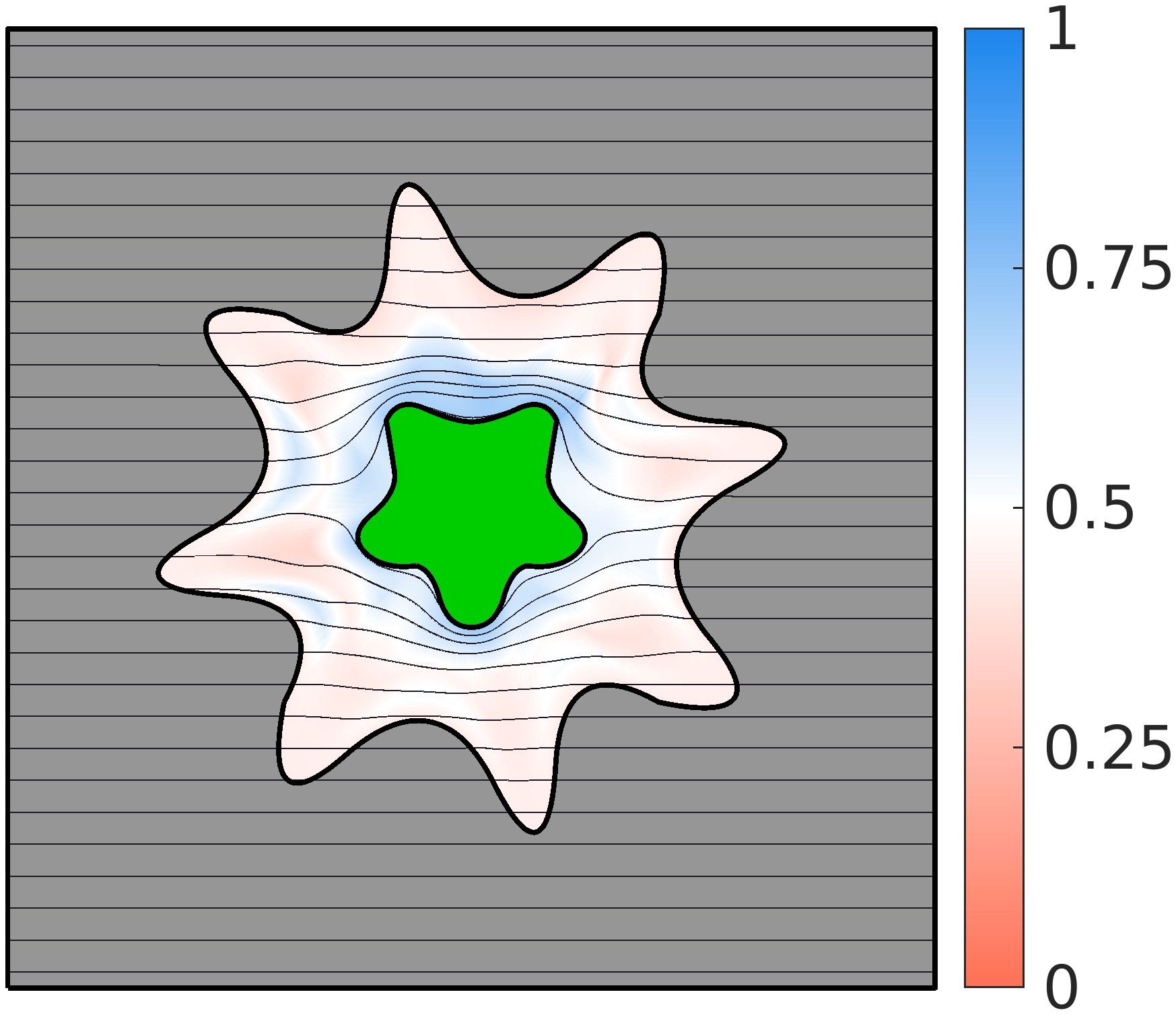
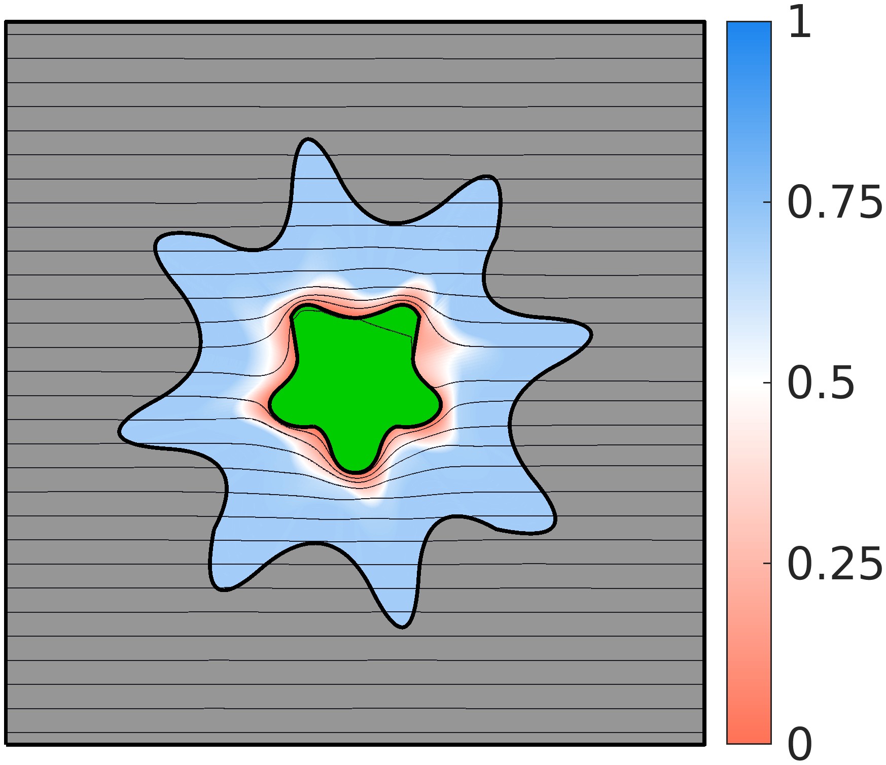
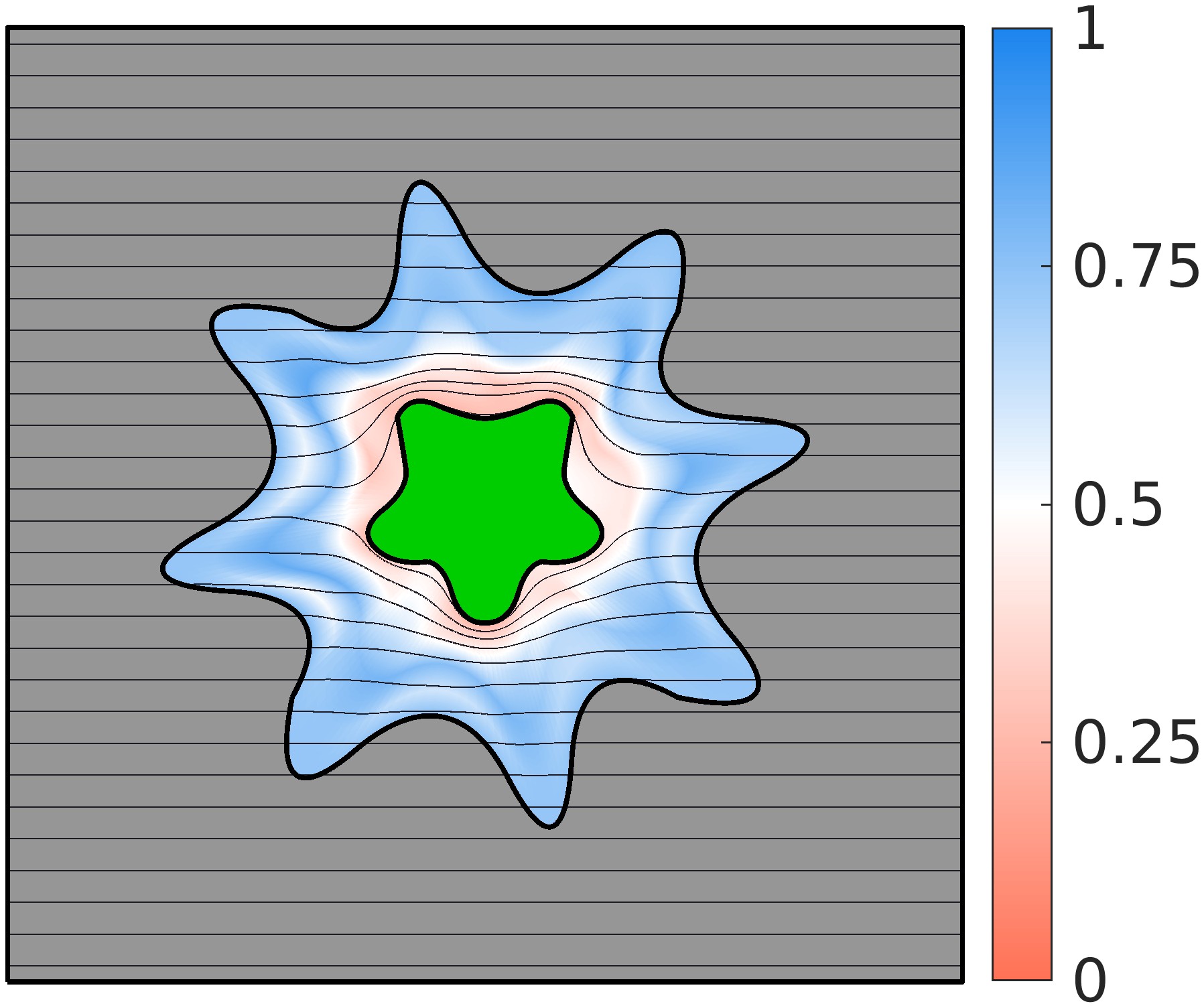
(a) Optimized material distribution	(b) Optimized material distribution	(c) Optimized material distribution
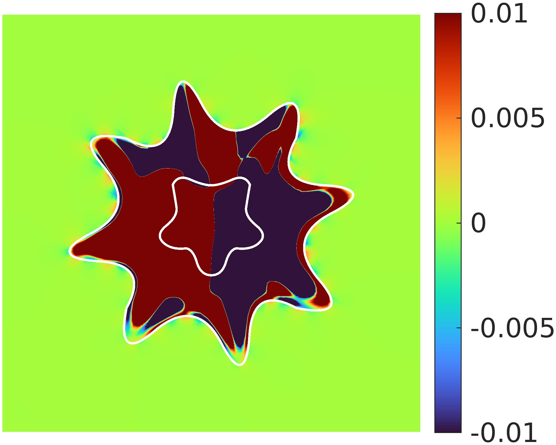
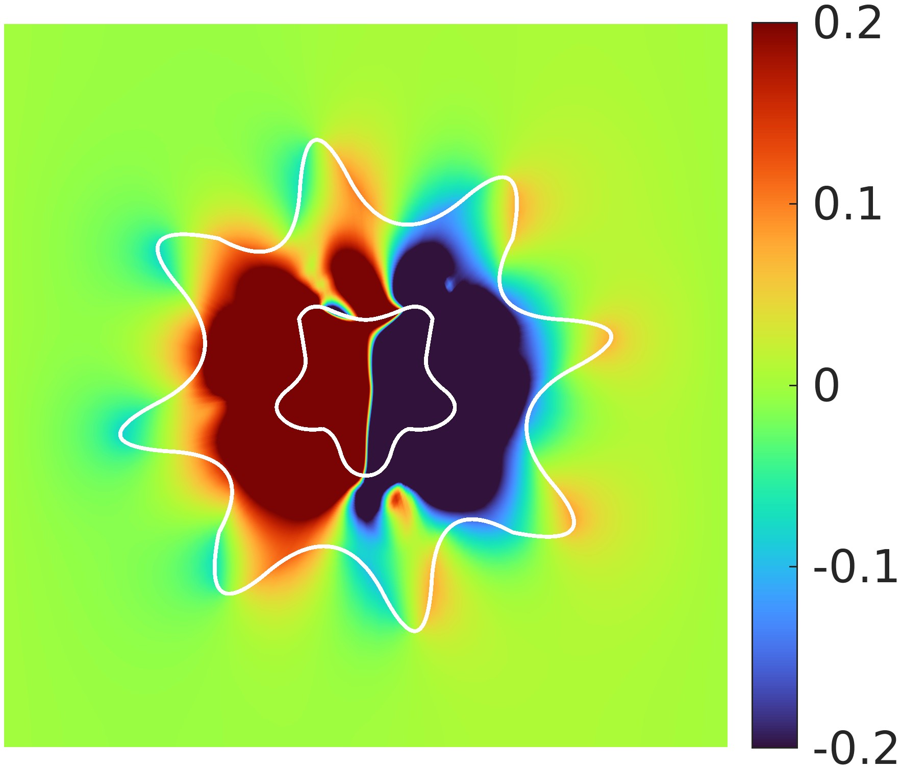
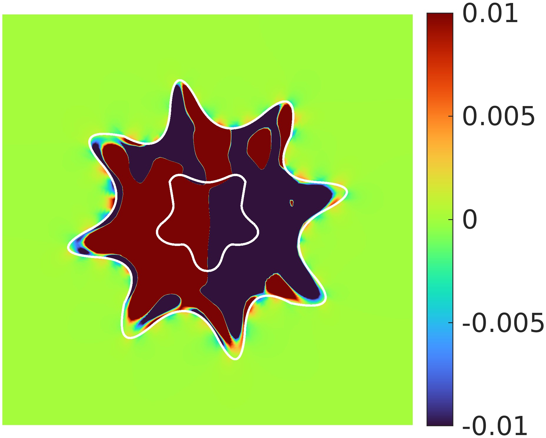
(d) $T-\overline{T}$,$J_{\rm cloak}=1.26\times 10^{-7}$	(e) $T-\overline{T}$,$J_{\rm cloak}=3.49\times 10^{-4}$	(f) $T-\overline{T}$, $J_{\rm cloak}=2.62\times 10^{-7}$

Figure 12: Optimized material distributions and temperature differences $T-\overline{T}$ for the thermal cloak problem with the star-shaped insulator and thermal cloak. Three material models (EMT, Porous Cu and Gyroid) and $N_{\rm var}=25$ are considered. Optimized objective function values are of order $10^{-4}$-$10^{-7}$.

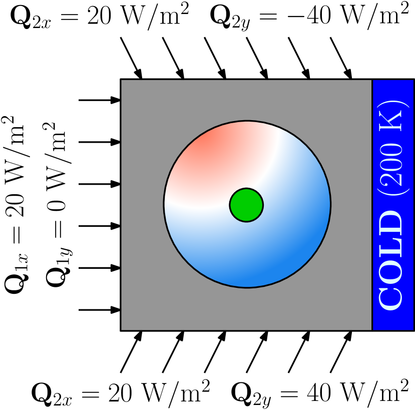
(a) Schematic of the thermal cloak problem under Neumann boundary condition.

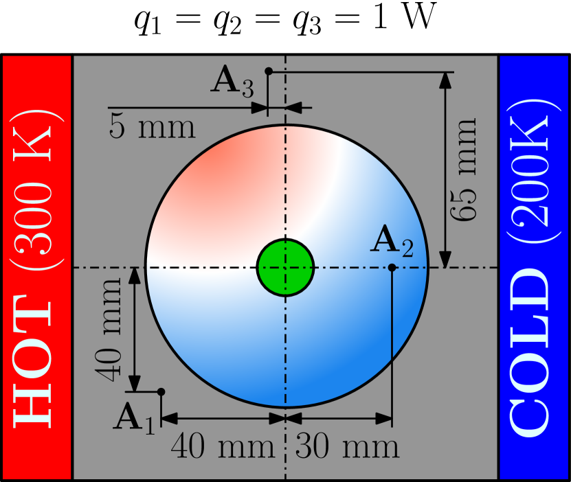
(b) Schematic of the thermal cloak problem with point heat sources in the domain.

Figure 13: Schematics of thermal cloak problems with various boundary conditions. Two cases (a) one with the Neumann boundary conditions, and (b) another with the point heat sources are considered. The specifics of boundary conditions are described in the schematics.

5.1.4 Design with various boundary conditions

In the next few paragraphs, we design the thermal cloaks under various boundary conditions. We solve two cases, one with Neumann boundary conditions, and another with point heat sources as shown in Figure 13. For the first problem, heat fluxes $\mathbf{Q}_{1}=[20,0]$ W/m², $\mathbf{Q}_{2}=[20,-40]$ W/m², and $\mathbf{Q}_{3}=[20,40]$ W/m² are applied on the left, top and bottom side, respectively. The right side is kept at $200$ K constant temperature. For the second problem, point heat sources $q_{i}=1$ W, $i=1,2,3$, are provided at the locations, $\mathbf{A}_{i}$, $i=1,2,3$. The right and left sides are kept at constant temperature $300$ K & $200$ K, respectively. For numerical analysis, the point heat sources are modelled as the domain heat source using approximate Dirac delta function $\widetilde{\delta}$. The total heat source $q_{b}$ can be can be written as follows:

$$q_{b}(\mathbf{x})=\sum_{i=1}^{3}q_{i}\widetilde{\delta}(||\mathbf{x}-\mathbf{A}_{i}||_{2})\quad\text{with}\quad\widetilde{\delta}(\phi)=\begin{cases}\dfrac{3}{4\Delta}\left(1-\dfrac{\phi^{2}}{\Delta^{2}}\right)\quad&\text{if}\quad\phi\leq\Delta\\ 0\quad&\text{if}\quad\phi>\Delta\end{cases}$$ (34)

where $\Delta$ is a support bandwidth. In this example, we take $\Delta=0.005$. For both problems, we consider three material models (EMT, Porous Cu and Gyroid) same as the last problem.

Reference case	EMT	Porous Cu	Gyroid
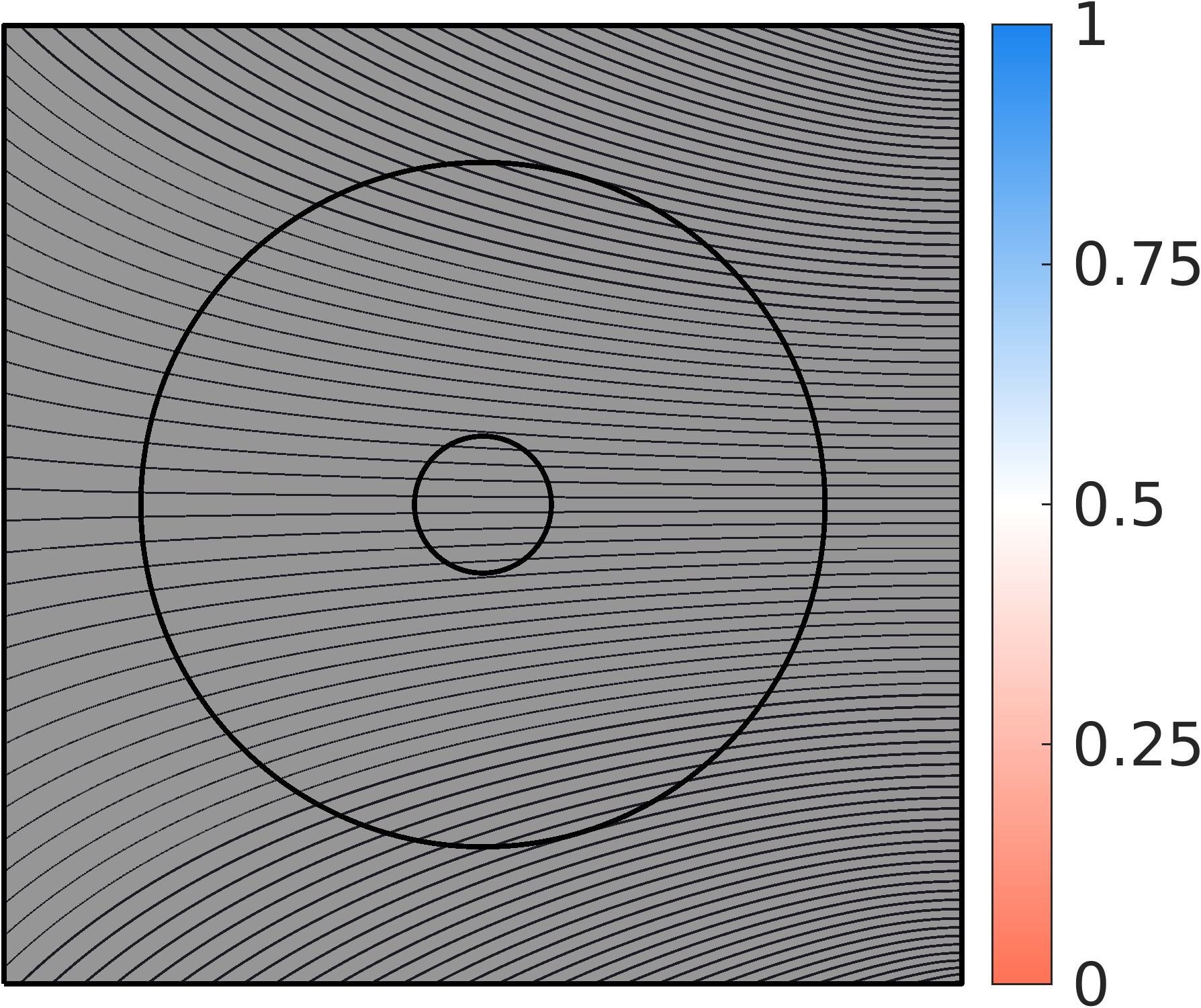
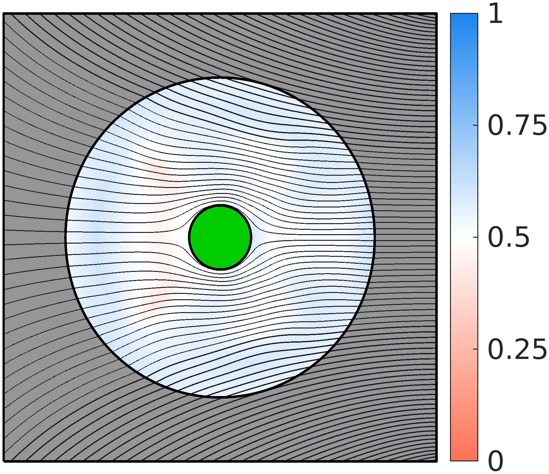
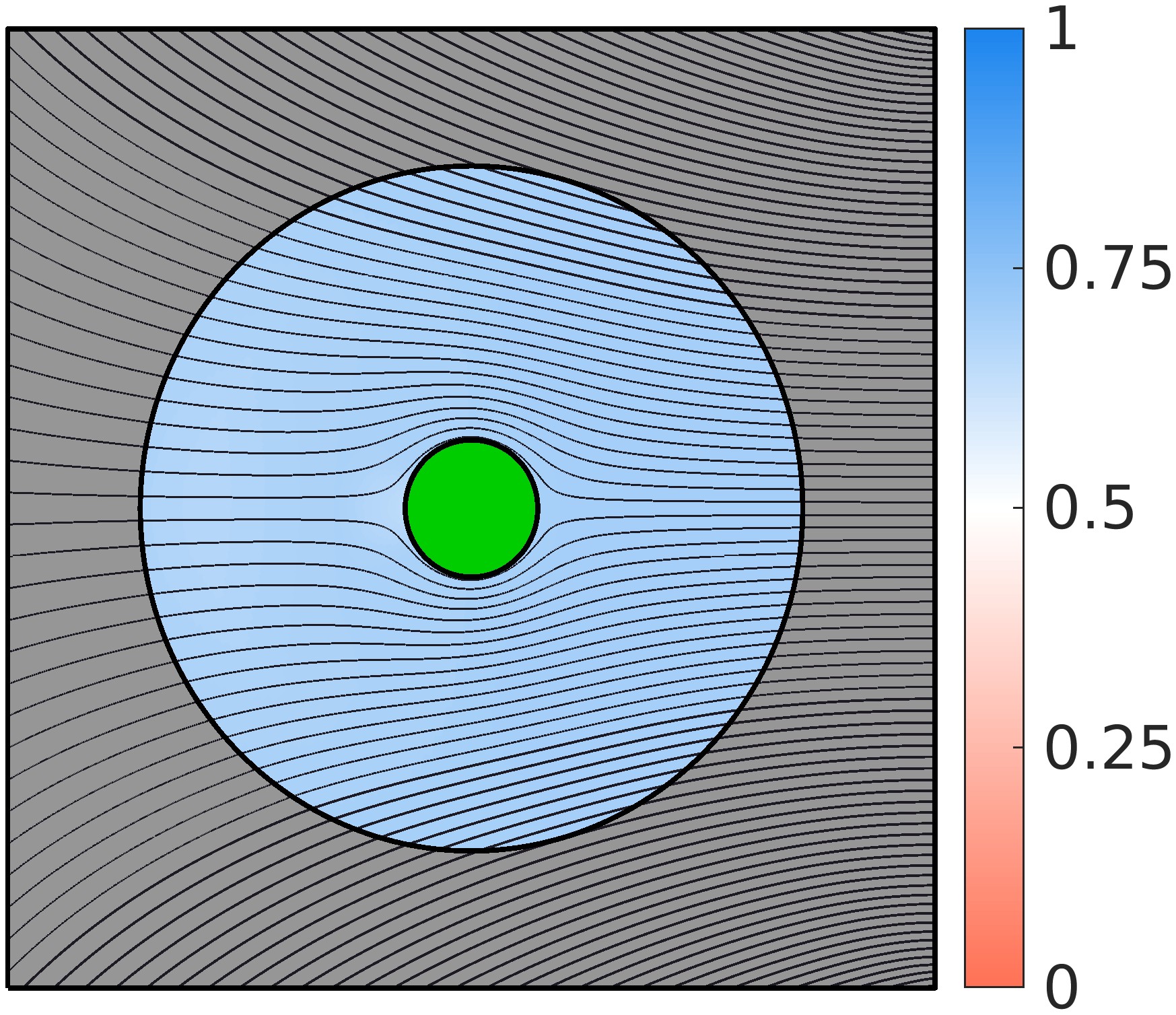
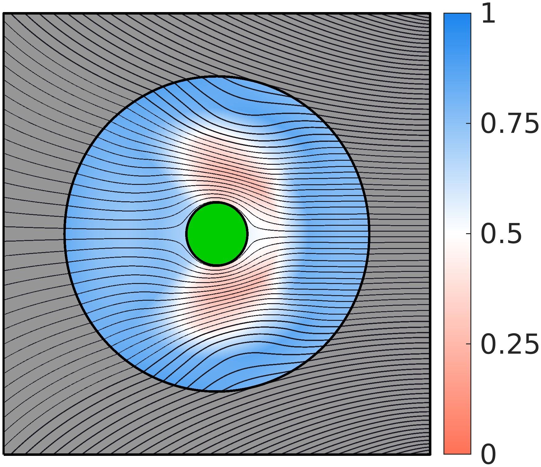
(a) Reference case	(b) Optimized material distribution	(c) Optimized material distribution	(d) Optimized material distribution
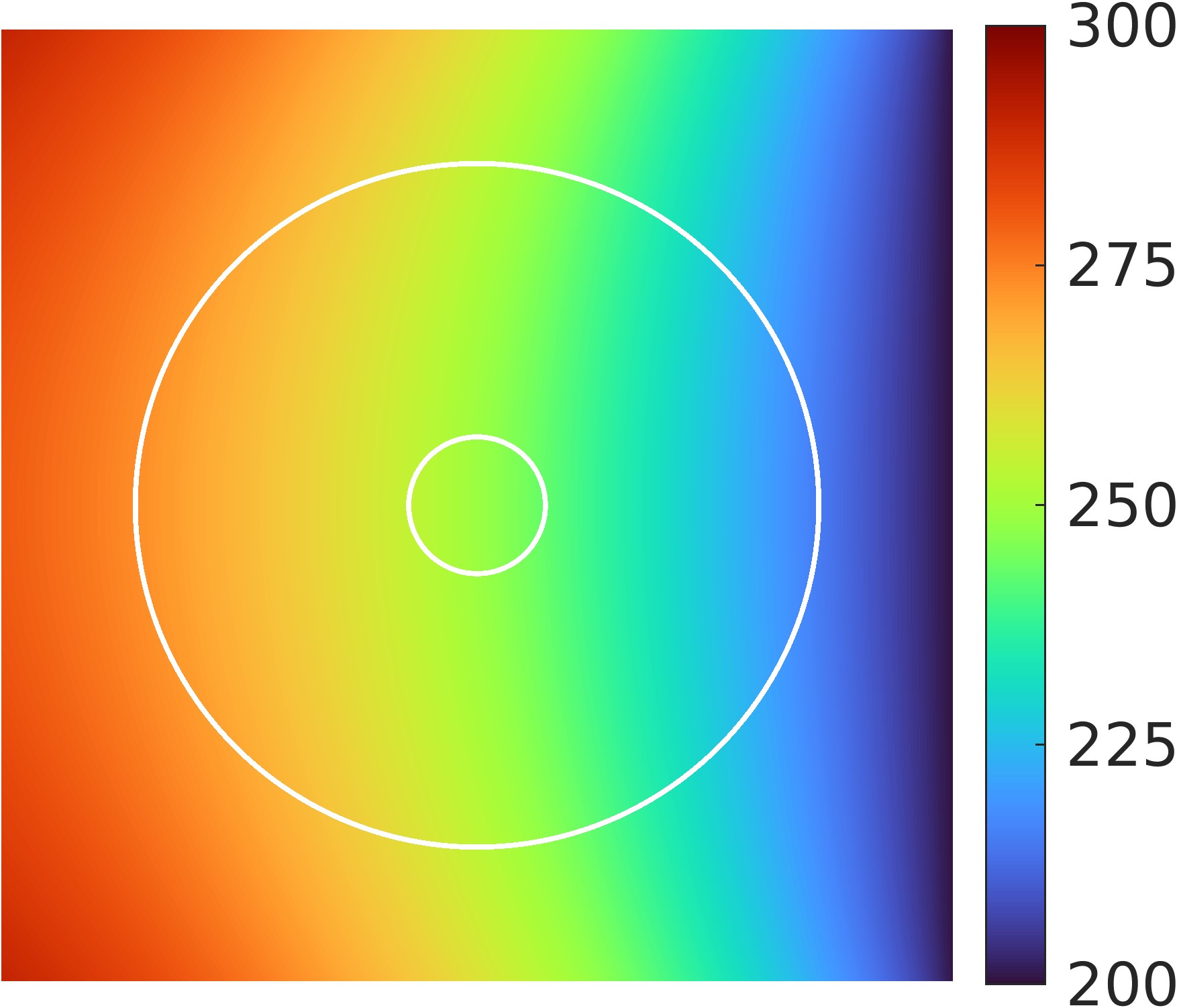
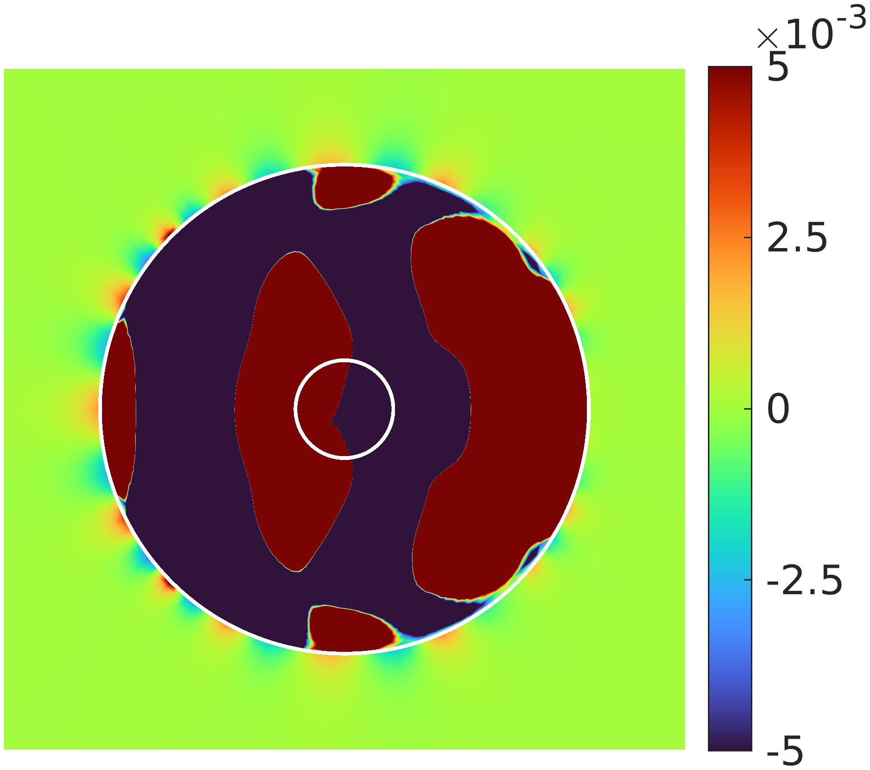
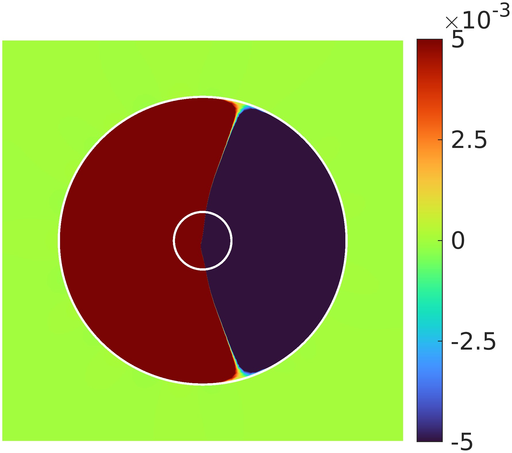
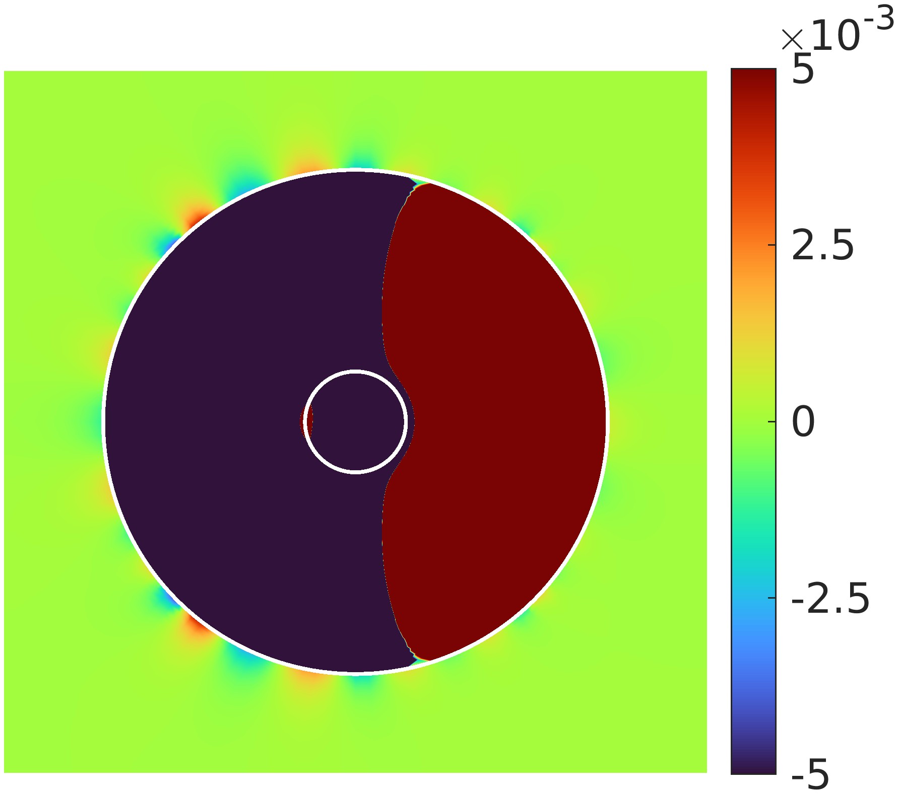
(e) Reference temp. distribution $\overline{T}$	(f) $T-\overline{T}$,$J=4.93\times 10^{-8}$	(g) $T-\overline{T}$,$J=9.51\times 10^{-11}$	(h) $T-\overline{T}$, $J=3.08\times 10^{-8}$

Figure 14: (Columns 2-4) Optimized material distributions and temperature differences $T-\overline{T}$ for the thermal cloak problem with Neumann boundary conditions. Three material models (EMT, Porous Cu and Gyroid) and $N_{\rm var}=25$ are considered. Optimized objective function values are of order $10^{-8}$-$10^{-11}$. Column 1 represents the reference case under applied boundary conditions.

The optimization results are shown in Figures 14-15. The proposed method can effectively design thermal cloaks for both problems with substantial cloaking function ($J_{\rm cloak}<10^{-6}$), except for Porous Cu model with point heat sources. As explained in the previous subsection, this is primarily due to a smaller $\kappa$-range for Porous Cu model. Improvements in $J_{\rm cloak}$ can be achieved by increasing design freedom or expanding the size of $\Omega_{\rm design}$.

Reference case	EMT	Porous Cu	Gyroid
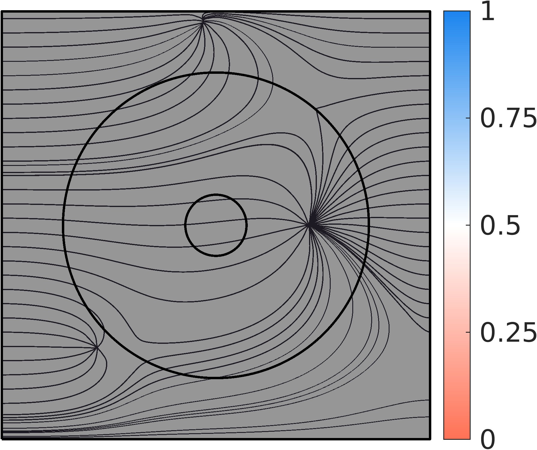
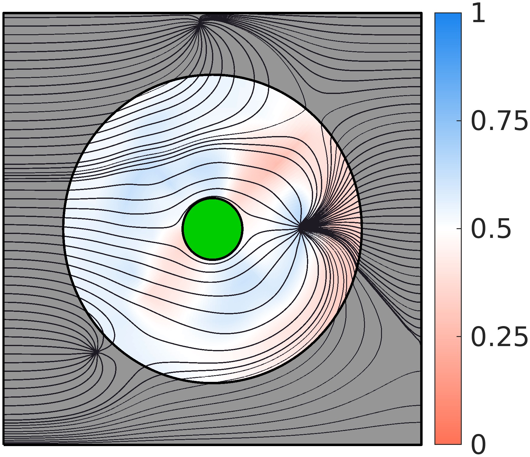
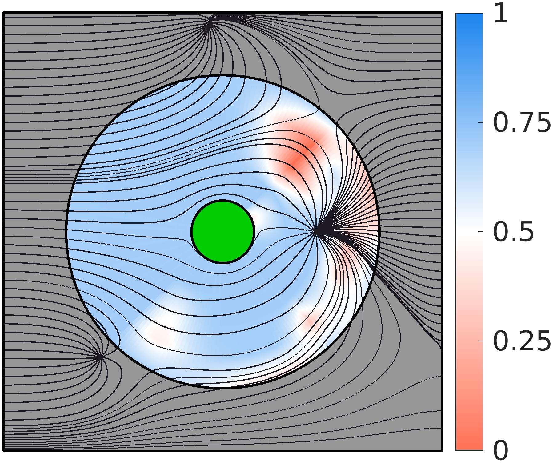
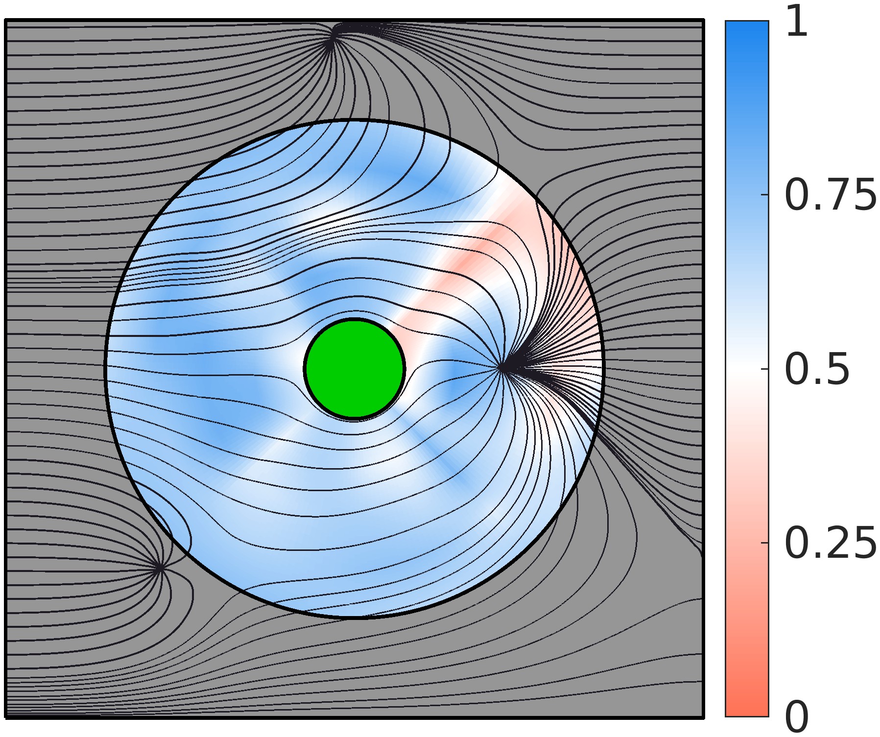
(a) Reference case	(b) Optimized material distribution	(c) Optimized material distribution	(d) Optimized material distribution
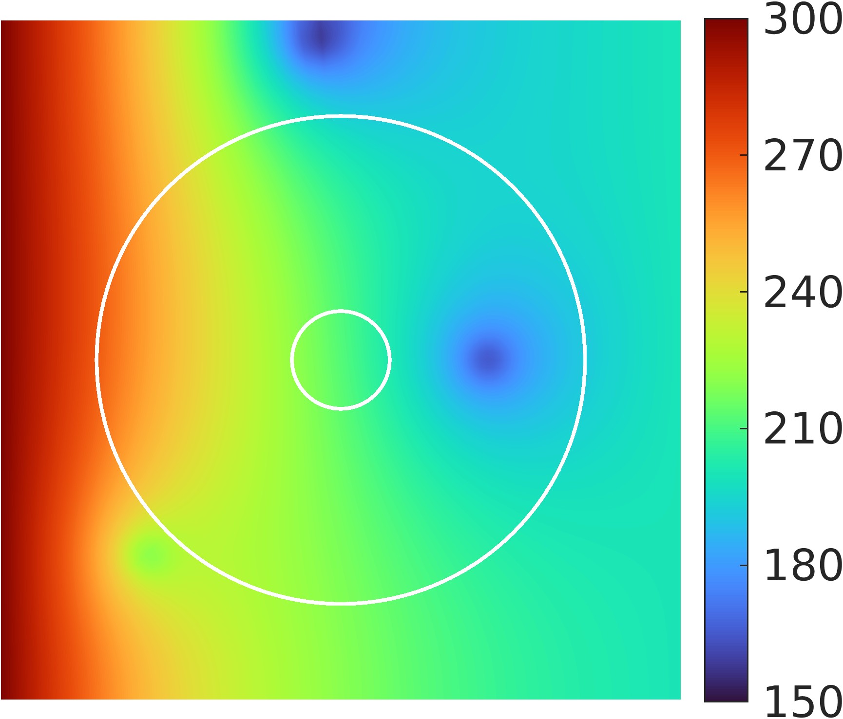
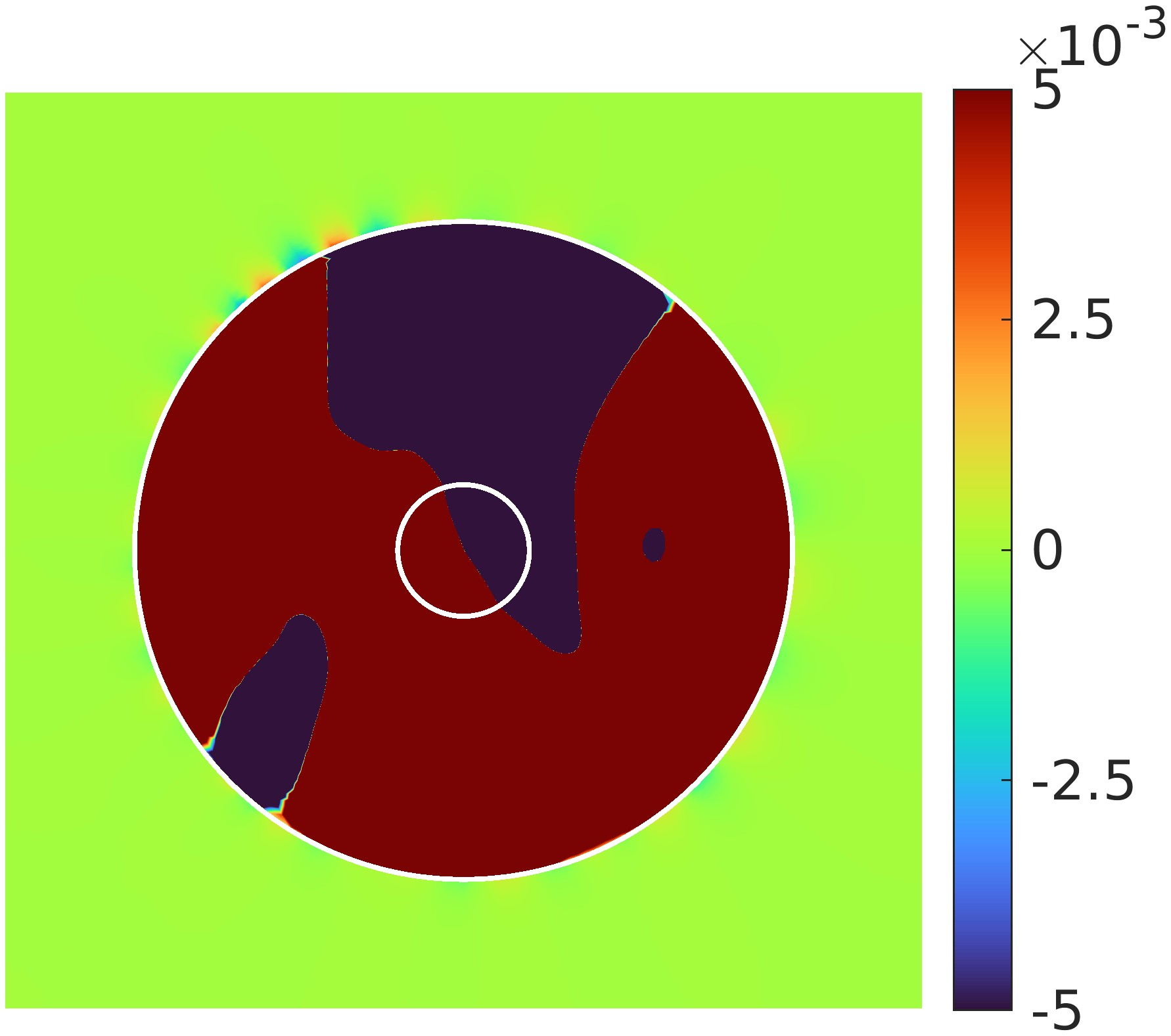
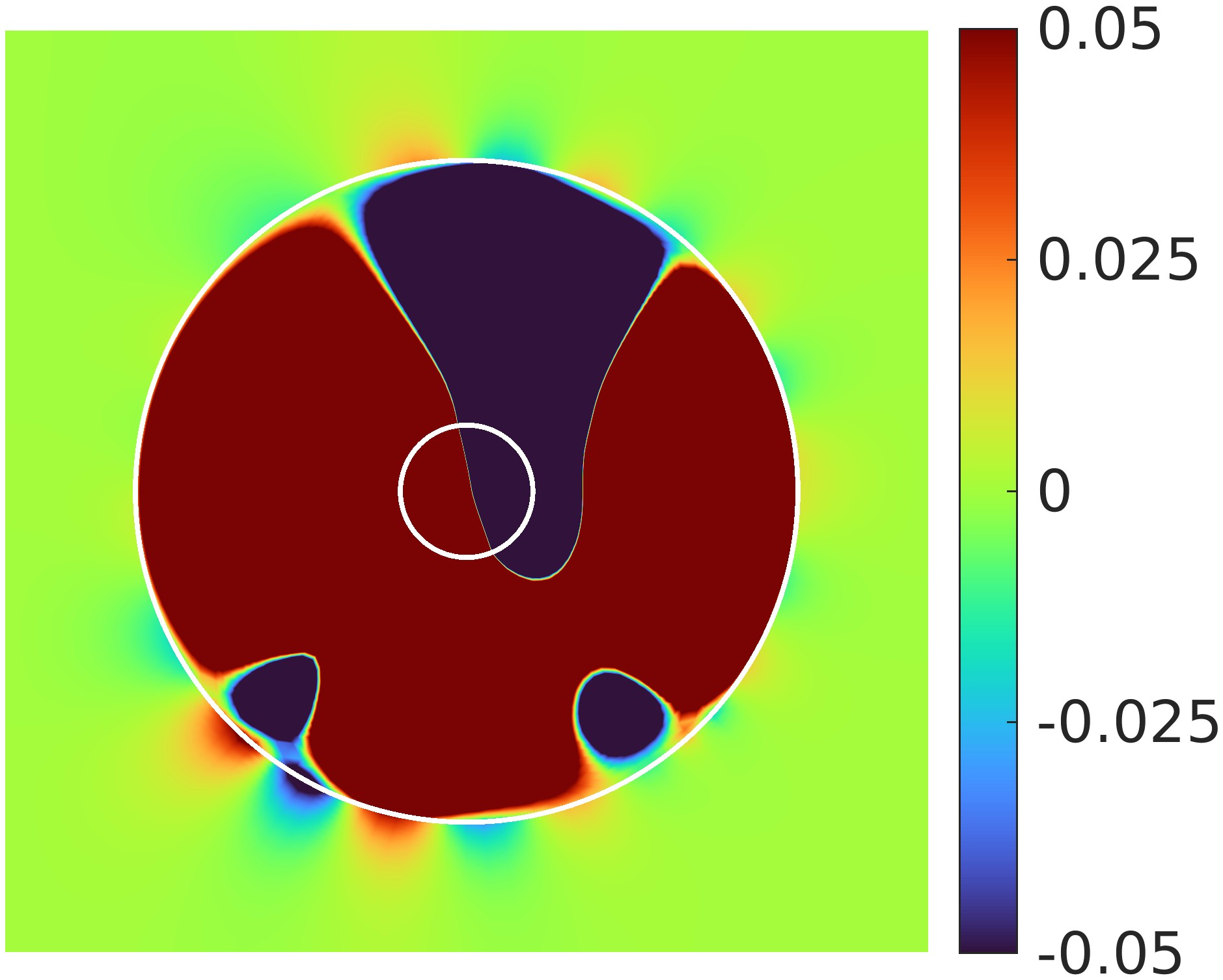
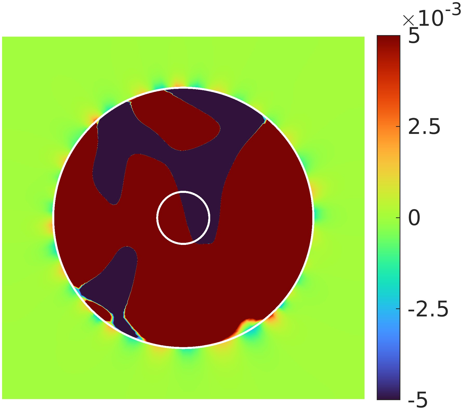
(e) Reference temp. distribution $\overline{T}$	(f) $T-\overline{T}$,$J=1.05\times 10^{-7}$	(g) $T-\overline{T}$,$J=1.19\times 10^{-4}$	(h) $T-\overline{T}$, $J=2.98\times 10^{-7}$

Figure 15: (Columns 2-4) Optimized material distributions and temperature differences $T-\overline{T}$ for the thermal cloak problem with the point heat sources inside the domain. Three material models (EMT, Porous Cu and Gyroid) and $N_{\rm var}=25$ are considered. Optimized objective function values are of order $10^{-4}$-$10^{-7}$. Column 1 represents the reference case under applied boundary conditions.

5.2 3D thermal cloak

In this subsection, we design 3D thermal cloaks using the proposed method. The geometry, boundary conditions and NURBS parameterizations are simple extensions of 2D problems as mentioned Section 5.1. The 3D cube of base material with embedded spherical insulator and thermal cloak is shown in Figure 16. All dimensions, conductivities, objective function and material distributions are assumed to be the same as those described in Section 5.1. For 3D thermal cloaks, we provide $x$, $y$ and $z$-plane symmetry for design meshes. Also, 3D problems are solved only on $\nicefrac{{1}}{{4^{th}}}$ domain (by giving symmetry conditions along $y$ & $z$-planes) to avoid the extra computational burden.

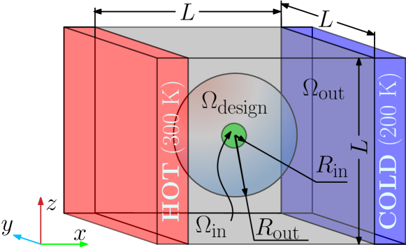
Figure 16: Schematics of a spherical insulator ($\mathrm{\Omega}_{\mathrm{in}}$) and a surrounding spherical FGM-based thermal cloak embedded ($\mathrm{\Omega}_{\mathrm{design}}$) in the base material cube $\mathrm{\Omega}$; $\mathrm{\Omega}_{\mathrm{design}}$ is the domain of the cloak where the material distribution is optimized, $\mathrm{\Omega}_{\mathrm{out}}$ is the outside domain of remaining base material, where the temperature disturbance is sought to be reduced. $\mathrm{\Omega}=\mathrm{\Omega}_{\mathrm{in}}\cup\mathrm{\Omega}_{\mathrm{design}}\cup\mathrm{\Omega}_{\mathrm{out}}$.

5.2.1 Design with various material models

EMT	Gyroid
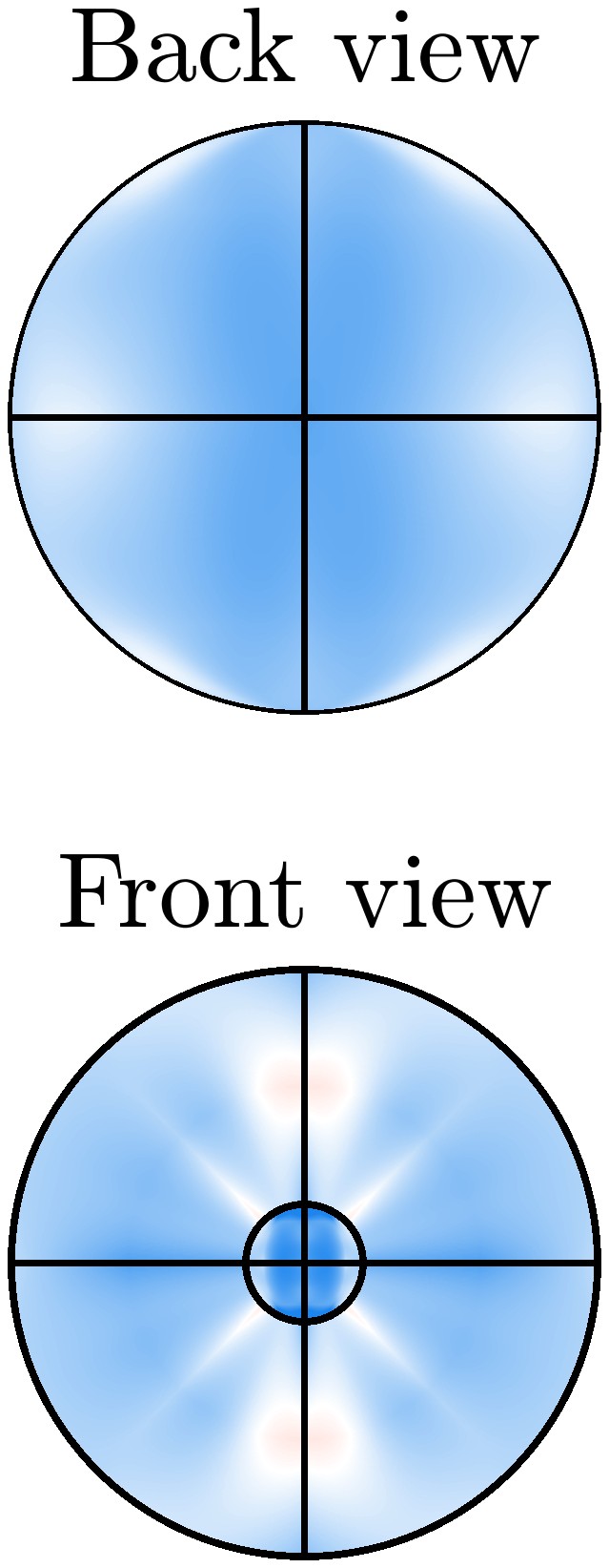
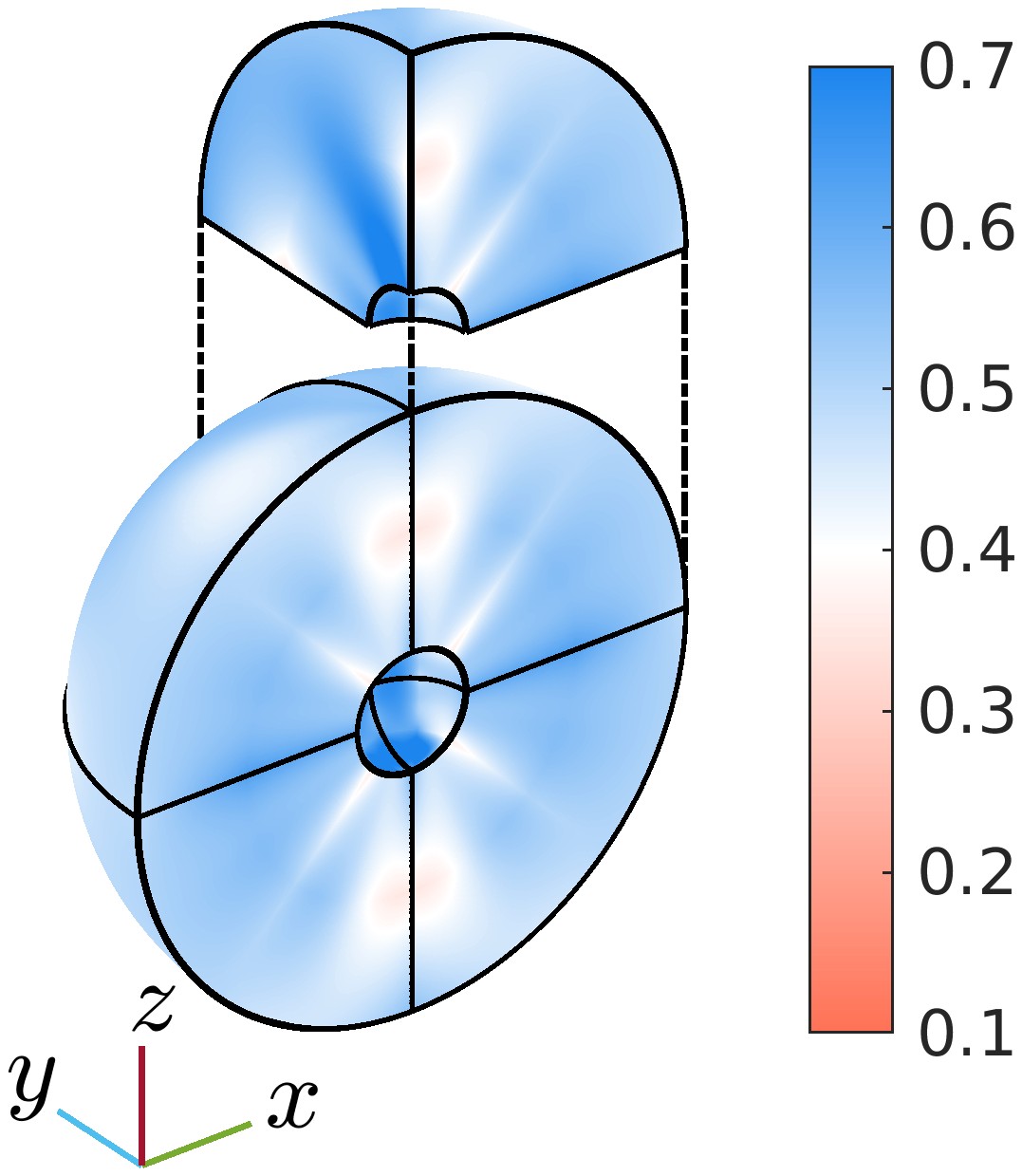
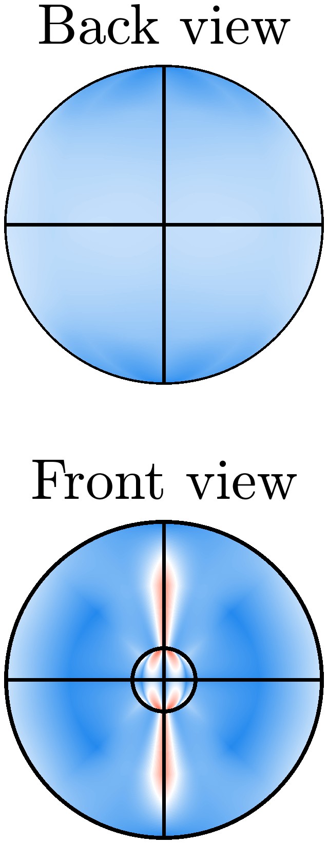
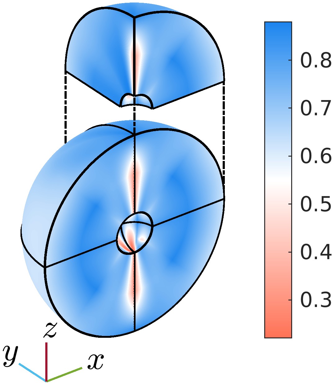
(a) $J_{\rm cloak}=1.23\times 10^{-3}$	(b) $J_{\rm cloak}=6.68\times 10^{-4}$

Figure 17: Optimized material distribution for the 3D thermal cloaks. Two material models (EMT and Gyroid) and $N_{\rm var}=129$ are considered. Optimized objective function values are of order $10^{-3}-10^{-4}$. Optimized material distributions remain close to the initial material distributions with almost the entire domain filled with intermediate densities.

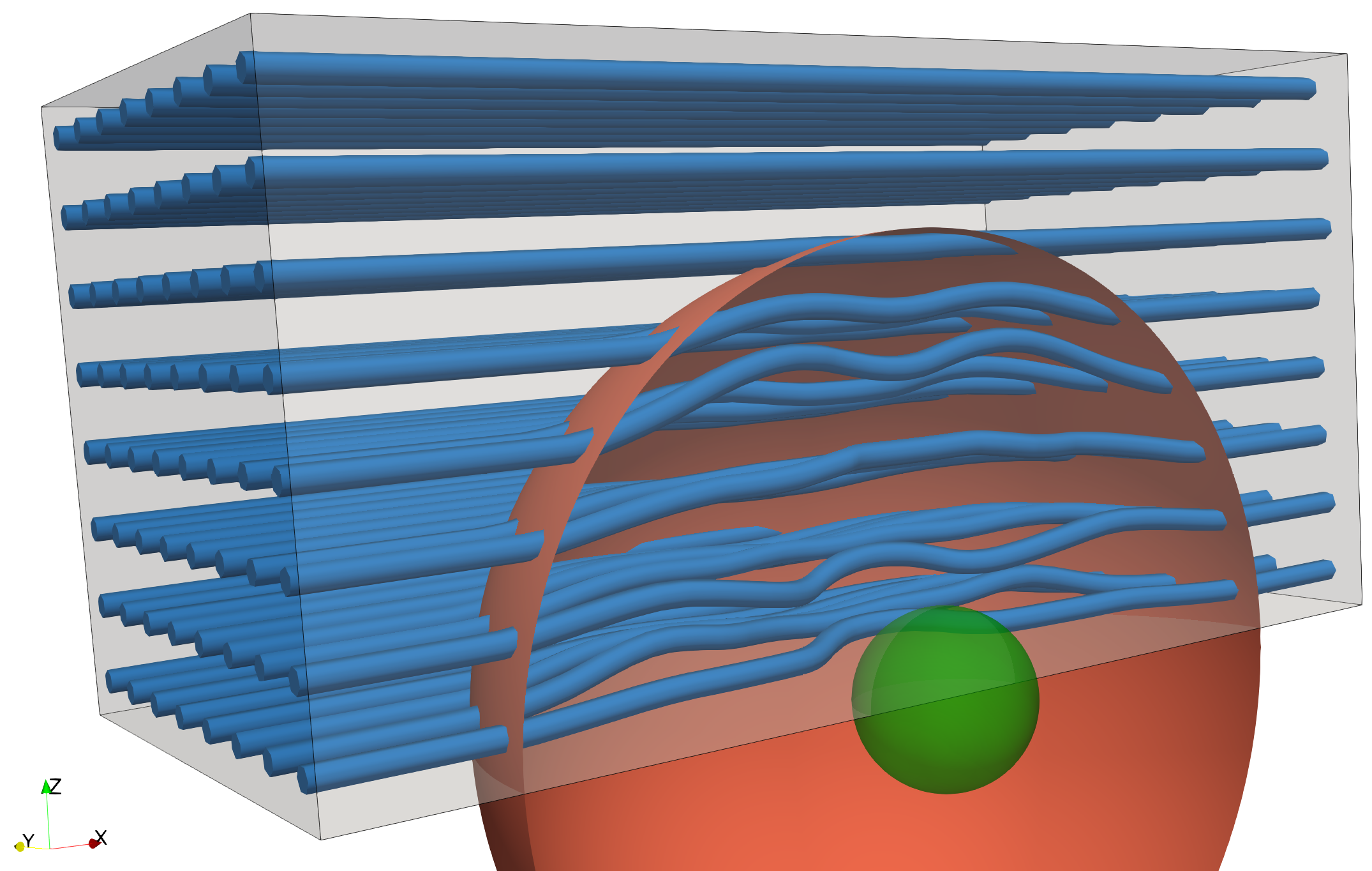
(a) Flux flow

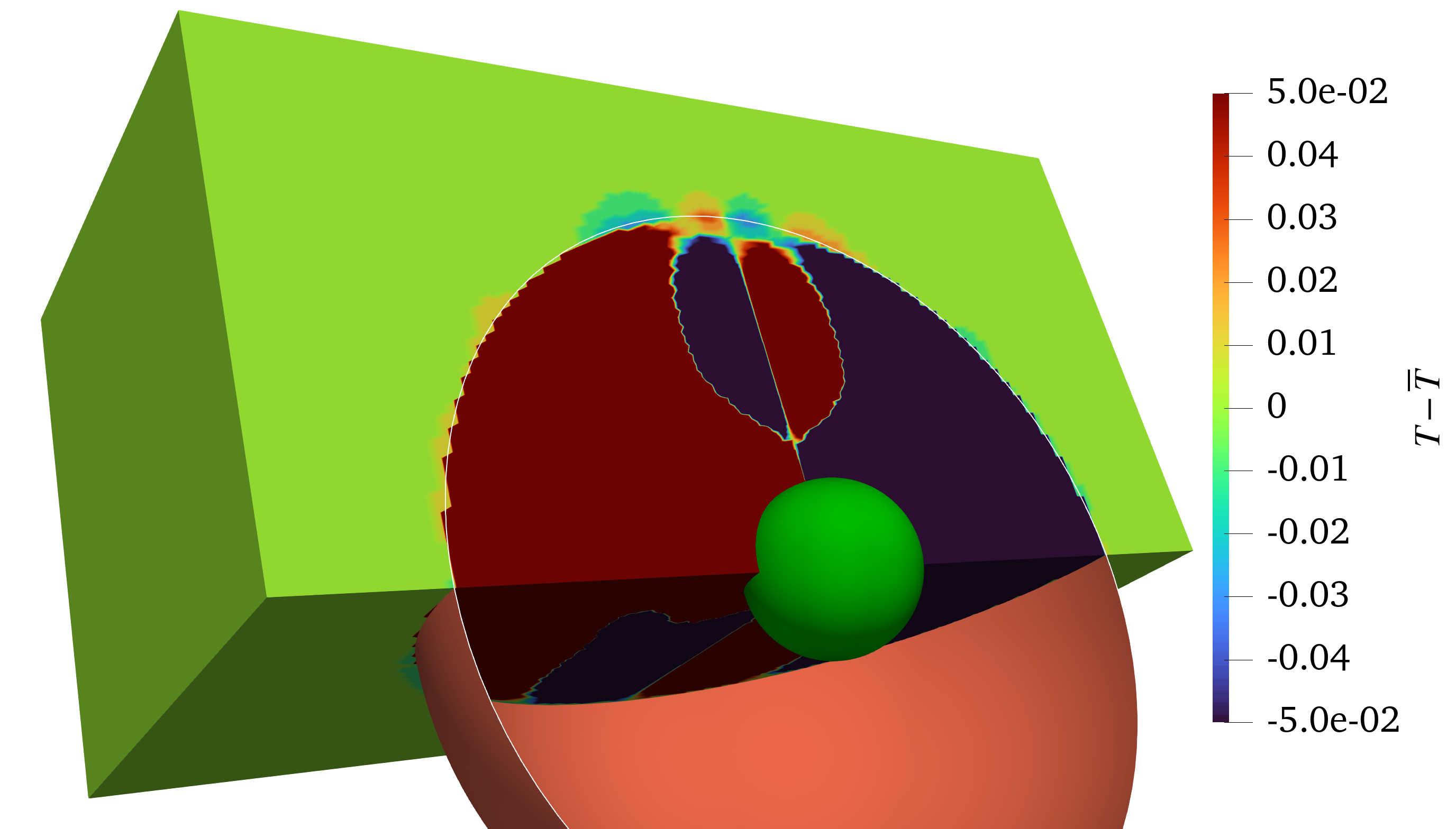
(b) Temperature difference $T-\overline{T}$

Figure 18: Flux flow and temperature difference (with respect to the reference case) $T-\overline{T}$ for the 3D thermal cloak. EMT model and $N_{\rm var}=129$ are considered. Optimized objective function value $J_{\rm cloak}=1.23\times 10^{-3}$. The 3D thermal cloak effectively diminishes the temperature disturbance in $\mathrm{\Omega}_{\mathrm{out}}$. The thermal cloak keeps the flux streamlines undisturbed and diminishes the temperature disturbance in $\mathrm{\Omega}_{\mathrm{out}}$. Temperature disturbances are almost nul in $\mathrm{\Omega}_{\mathrm{out}}$, even with the 3-order smaller temperature range.

The optimized material distributions of thermal cloaks design with two material models (EMT and Gyroid) are shown in Figure 17. We use a design mesh with $N_{\rm var}=129$ and a solution mesh with DOF=124950. Similar to 2D thermal cloaks, the optimizations settle to the nearest local solutions for 3D thermal cloaks. Optimized material distributions reach the objective function value of order $10^{-3}-10^{-4}$. The material distribution varies slightly according to each material law and its limits on relative density, $v_{\rm min}$ & $v_{\rm max}$. We exhibited the cloaking performance of the thermal cloak obtained using EMT in Figure 18. The figure presents the flux flow and temperature difference with respect to a homogeneous base material plate. From the figure, it is observed that the optimized thermal cloaks diminish the temperature disturbance in $\Omega_{\rm out}$. Temperature difference $T-\overline{T}$ is almost negligible in $\Omega_{\rm out}$ in the temperature range which is 3 orders smaller than actual temperature values.

5.2.2 Design with free-form geometries

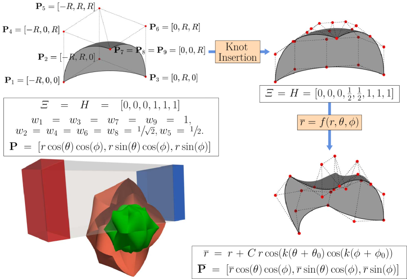
Figure 19: Steps to generate the star-shaped 3D insulator & 3D thermal cloak and schematics of the final domain. The control points related to the circumferential parametric directions of the sphere of radius $R_{\rm in}$ and $R_{\rm out}$ are perturbed. The steps for perturbation are as follows: (i) $\nicefrac{{1}}{{4^{th}}}$ of a NURBS-sphere is created using the knot vectors $\Xi=H=[0,0,0,1,1,1]$ with nine control points $\mathbf{P}_{i}$, $i=1,2,...,9$. The Cartesian coordinates and weights of the control points are shown in the first figure. (ii) The NURBS-geometry is refined by adding knots $\nicefrac{{1}}{{2}},\nicefrac{{1}}{{2}}$ through the knot insertion procedure in both $\Xi$ and $H$. (iii) The control points of the refined geometry are transformed into spherical coordinates $(r,\theta,\phi)$ from Cartesian coordinates $\mathbf{P}=(x,y,z)$; the radial coordinates $r$ are perturbed by the function, $\overline{r}=r+Cr\cos{(k(\theta+\theta_{0}))}\cos{(k(\phi+\phi_{0}))}$, while keeping $\theta$ and $\phi$ coordinates unchanged; the modified spherical coordinates $(\overline{r},\theta,\phi)$ are transformed back into Cartesian coordinates $\overline{\mathbf{P}}=(\overline{x},\overline{y},\overline{z})$. For $R_{\rm in}=25$ mm, $C=0.3$, $k=5$, $\theta_{0}=\pi$ and $\phi_{0}=0$, while for $R_{\rm out}=50$ mm, $C=0.2$, $k=4$, $\theta_{0}=-\pi$ and $\phi_{0}=\pi$. The entire geometry is created then using symmetry conditions along $y$-and $z$-planes.

In this subsection, we check a free-form geometry for a 3D thermal cloak and insulator. Similar to 2D free-form geometries as in Section 5.1.3, we define the free-form-shaped 3D insulator and thermal cloak by the method of perturbation. We consider the geometry to be symmetric along all three axes, and only $\nicefrac{{1}}{{8^{th}}}$ part of spheres of radius $R_{\rm in}=25$ mm and $R_{\rm out}=50$ mm are taken into account for perturbation. Later, the knot insertion, coordinate-system transformations (from Cartesian to spherical & from spherical to Cartesian) and functional transformation of radial coordinates are performed to perturb their control points. The detailed procedure is presented in Figure 19. We use $C=0.3$, $k=5$ $\theta_{0}=\pi$ and $\phi_{0}=0$ for $R_{\rm in}=25$ mm, while $C=0.2$, $k=4$ $\theta_{0}=\pi$ and $\phi_{0}=\pi$ for $R_{\rm in}=50$ mm. To create overall $\nicefrac{{1}}{{4^{th}}}$ of the entire geometry for numerical analysis, the mirror images of both spheres are taken along $x$-plane. The final domain created for the problem is also shown in Figure 19. The results of the optimization are presented in Figure 5.1.1. From the figure, we can observe that the material distribution presented in Figure 20(a) diminishes the temperature disturbance created by the insulator with the objective function value $J=2.35\times 10^{-5}$. Also, the flux flow shows undisturbed, parallel to $x$-axes streamlines in $\Omega_{\rm out}$ region.

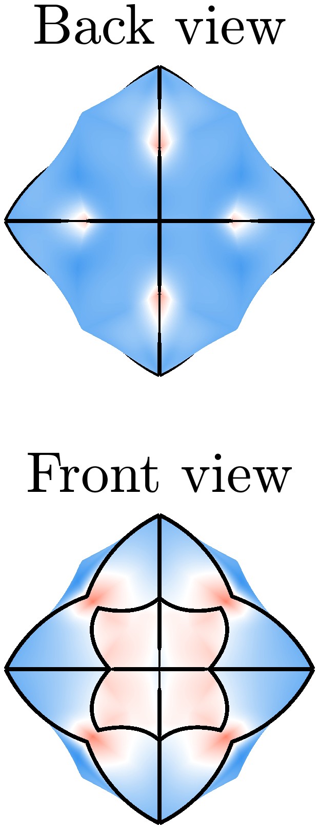
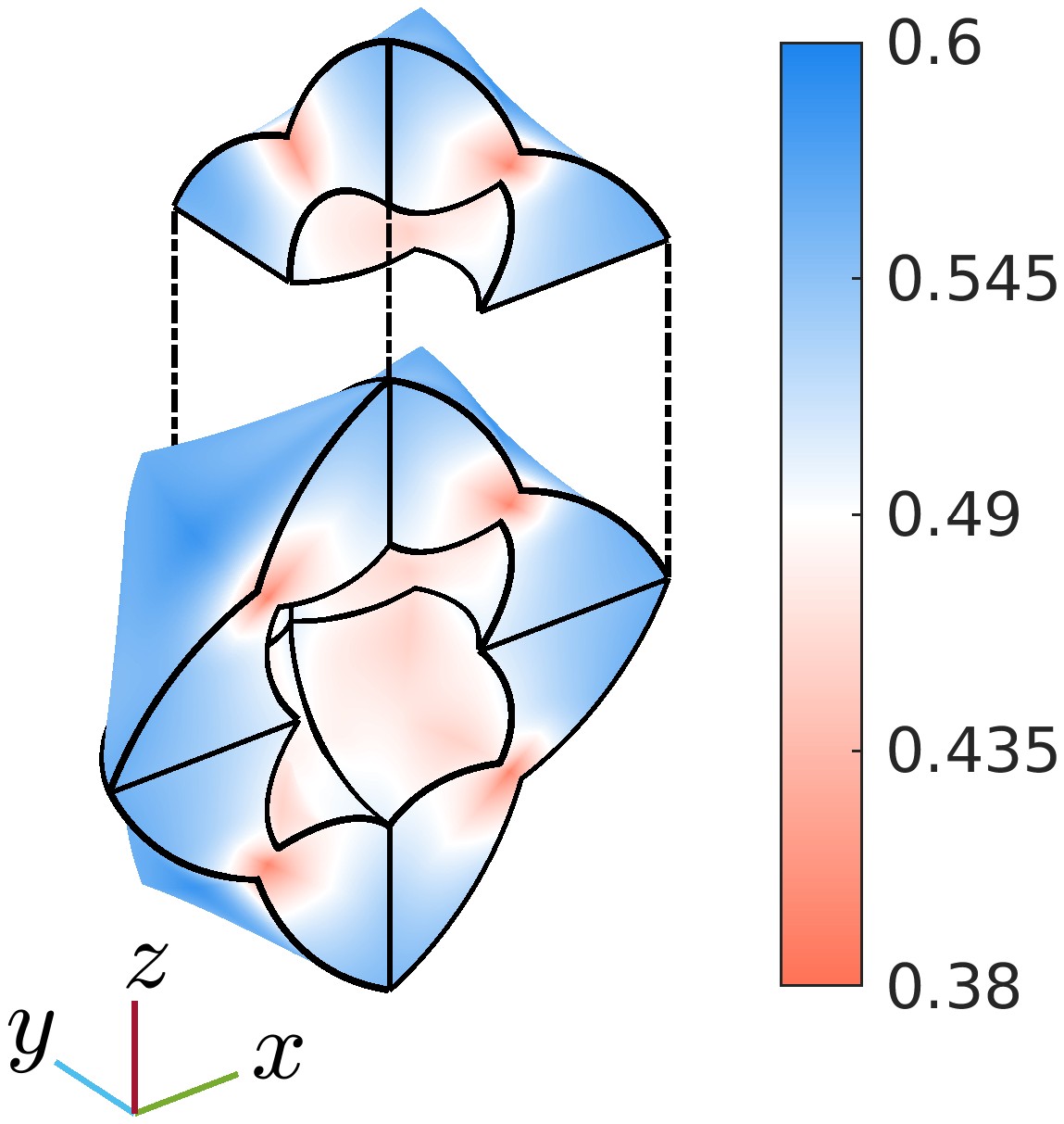
(a) Optimized material distribution

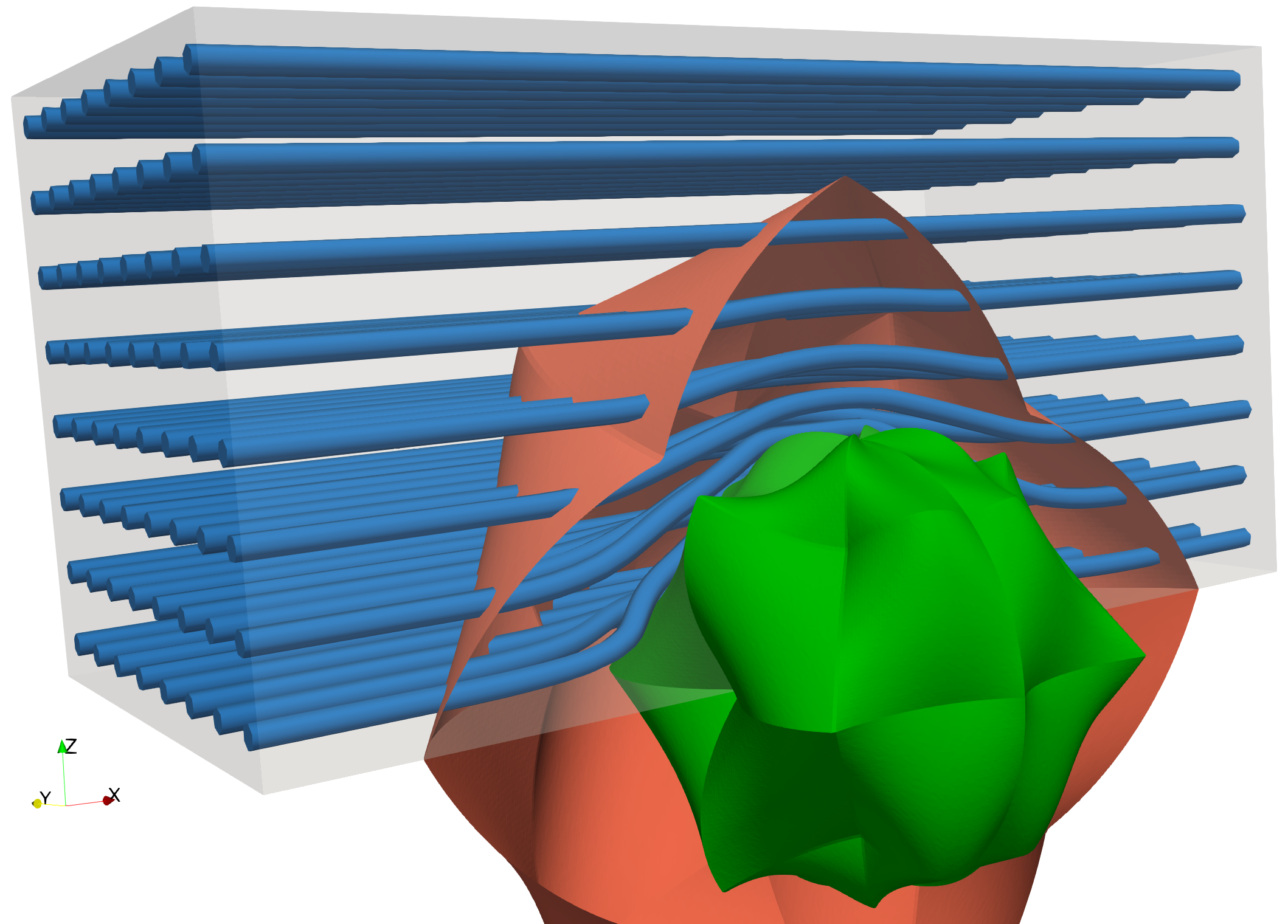
(b) Flux flow

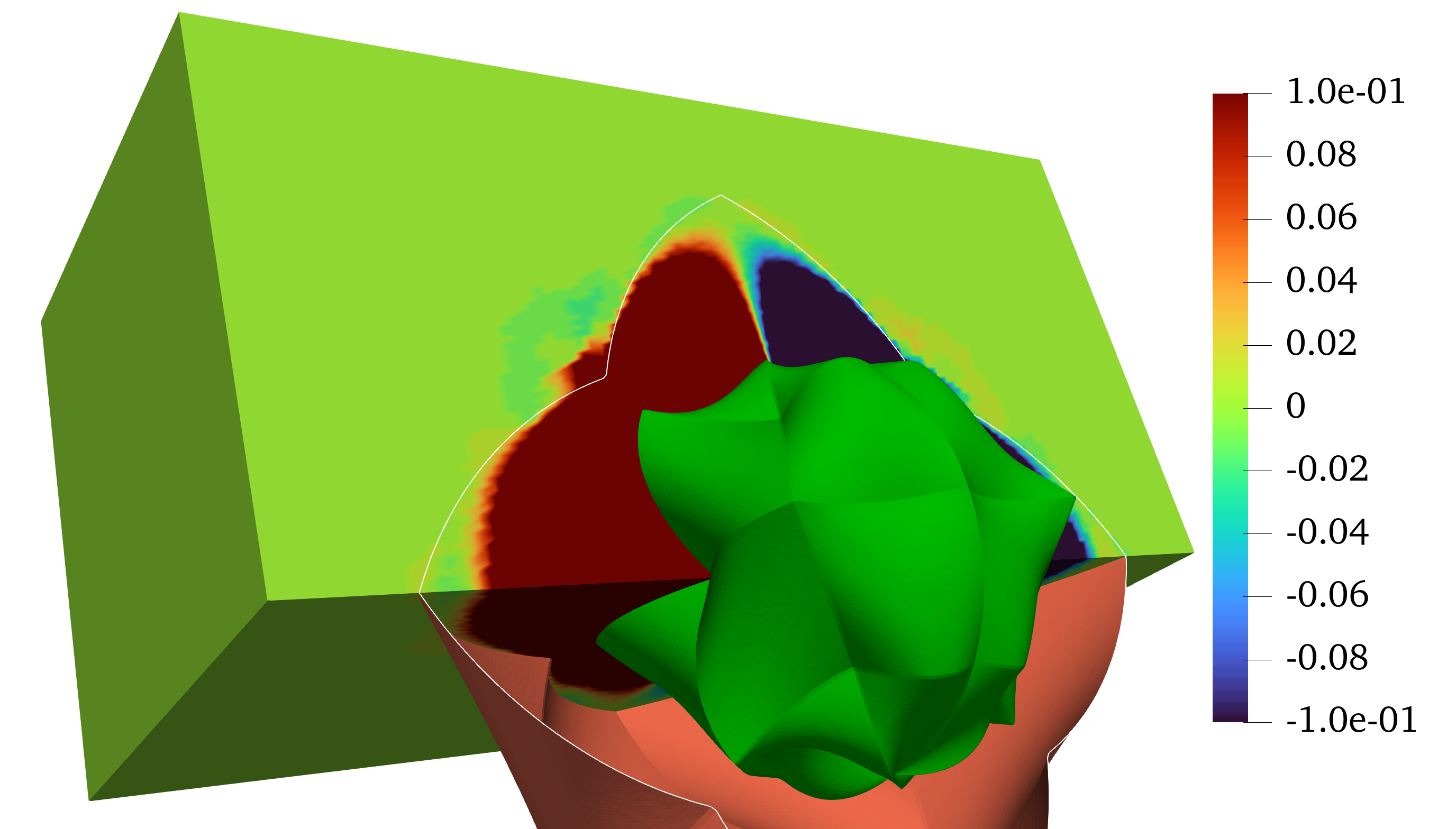
(c) Temperature difference $T-\overline{T}$

Figure 20: Optimized material distribution, flux flow and temperature difference (with respect to the reference case) $T-\overline{T}$ for the 3D thermal cloak problem with complex shaped insulator and thermal cloak. EMT model and $N_{\rm var}=129$ are considered. Optimized objective function value $J_{\rm cloak}=2.35\times 10^{-5}$. The 3D thermal cloak keeps the flux streamlines undisturbed and diminishes the temperature disturbance in $\mathrm{\Omega}_{\mathrm{out}}$. Temperature disturbances are almost nil in $\mathrm{\Omega}_{\mathrm{out}}$, even with the 3-order smaller temperature range.

6 Other thermal meta-structures

In this section, we investigate various other thermal meta-structures such as thermal concentrators, thermal rotators, thermal cloaking sensors, thermal cloaking concentrators and thermal bidirectional cloak-concentrators. Each of these manipulators is associated with a distinct objective function. For all manipulators, we take an geometry identical to that of the thermal cloak problem as depicted in Figure 4 for 2D cases and in Figure 16 for 3D cases. The dimensions and material allocations can vary example-wise, which will be mentioned in their respective descriptions.

6.1 Thermal concentrator

In this example, we design both 2D and 3D thermal concentrators. For the concentrator, we consider the same dimensions and boundary conditions as the thermal cloak problem. Even the materials involved are the same with only differences in their allocation. In this thermal meta-structure, $\Omega_{\rm in}$ is filled with the base material iron instead of the insulator.

The objective of a thermal concentrator is to concentrate the flux inside region $\Omega_{\rm in}$. Thus, we define the concentration function in a mathematical sense as follows:

$$\varPsi_{\mathrm{cntr}}=\dfrac{1}{\widetilde{\varPsi}_{\mathrm{cntr}}}\int_{\Gamma_{\mathrm{in}}}-\kappa_{\mathrm{in}}\nabla T\cdot\mathbf{n}~d\Gamma,\quad\text{with}\quad\widetilde{\varPsi}_{\mathrm{cntr}}=\int_{\Gamma_{\mathrm{in}}}-\overline{\kappa}_{\mathrm{in}}\nabla\overline{T}\cdot\mathbf{n}~d\Gamma,$$ (35)

where $\overline{T}$ is the temperature when entire $\mathrm{\Omega}$ is filled with the base material. From a physical perspective, the concentration function value represents the concentrated flux as a multiple of the flux in the homogeneous base plate case. Since we solve the minimization problem in optimization, the original objective function is defined as the inverse of the absolute value of a concentration function, $J_{\rm cntr}=\dfrac{1}{\varPsi_{\mathrm{cntr}}}$. Before running the optimizations, we also perform a mesh sensitivity analysis and take a mesh with DOF=13167 as the solution mesh, similar to Section 5.1 . The results of the mesh sensitivity analysis are also presented in B.

EMT
$v_{i}\in[0,1]$	Maxwell
$v_{i}\in[0,1]$	Porous Cu
$v_{i}\in[0,0.7]$	Cu-Sn-Pb
$v_{i}\in[0,0.3]$	TCOH
${v_{i}\in[0.2,0.8]}$	Gyroid
$v_{i}\in[0.2,0.9]$
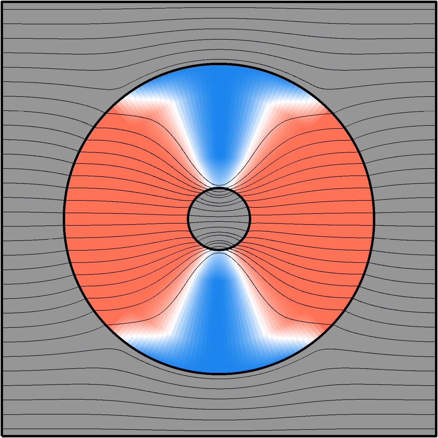
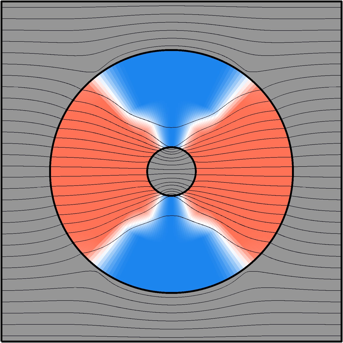
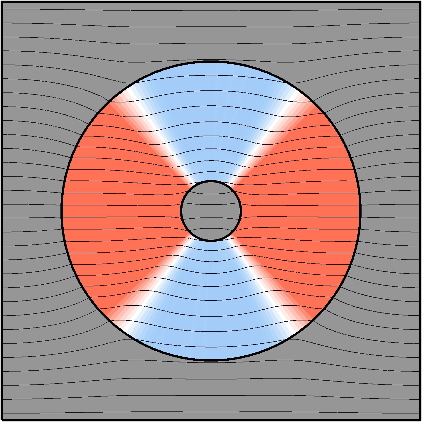
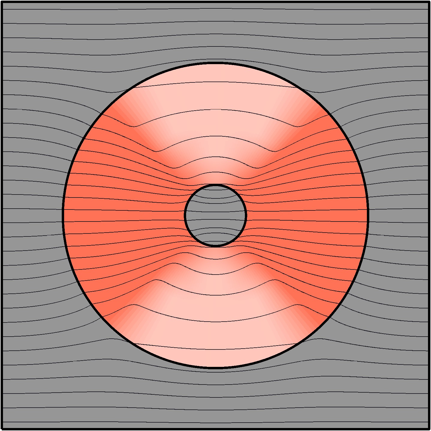
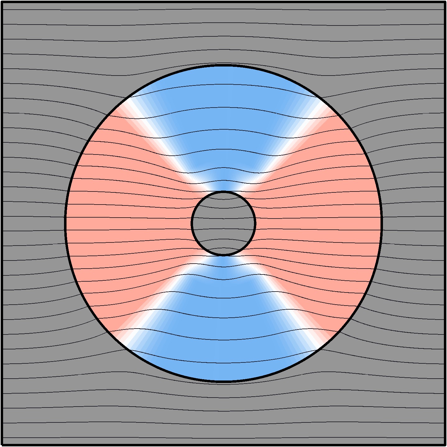
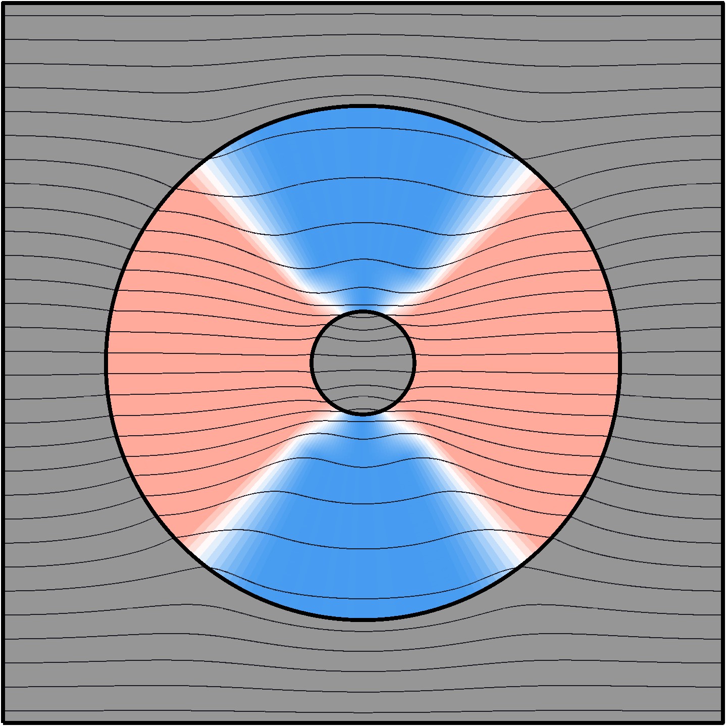
(a) $N_{\rm var}=25$, $J=2.19\times 10^{-1}$, $\varPsi_{\rm cntr}=4.57$	(b) $N_{\rm var}=25$, $J=2.27\times 10^{-1}$, $\varPsi_{\rm cntr}=4.41$	(c) $N_{\rm var}=25$, $J=4.72\times 10^{-1}$, $\varPsi_{\rm cntr}=2.12$	(d) $N_{\rm var}=25$, $J=3.35\times 10^{-1}$, $\varPsi_{\rm cntr}=2.98$	(e) $N_{\rm var}=25$, $J=4.34\times 10^{-1}$, $\varPsi_{\rm cntr}=2.31$	(f) $N_{\rm var}=25$, $J=3.72\times 10^{-1}$, $\varPsi_{\rm cntr}=2.69$
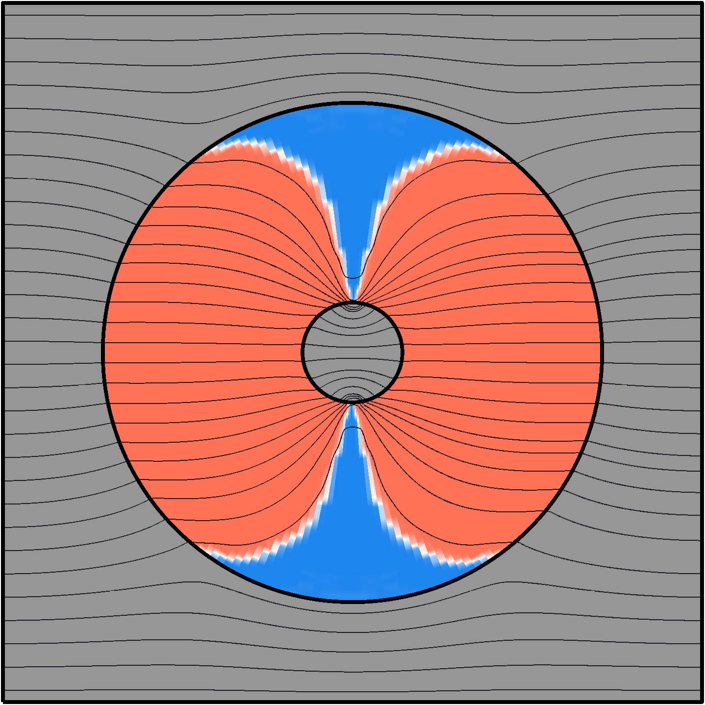
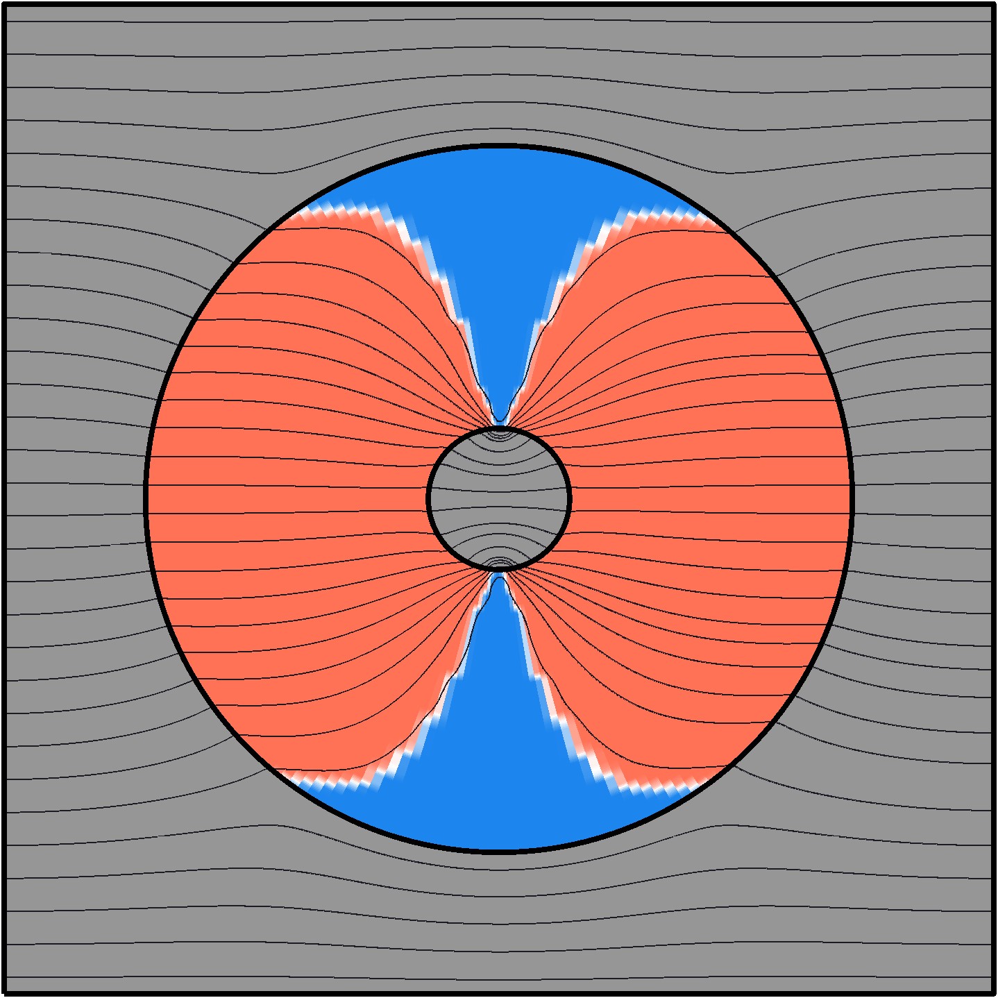
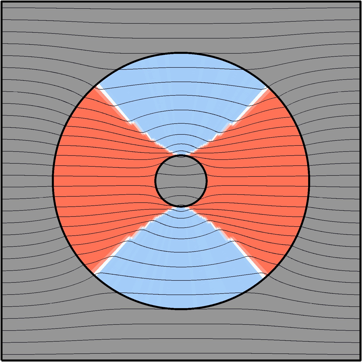
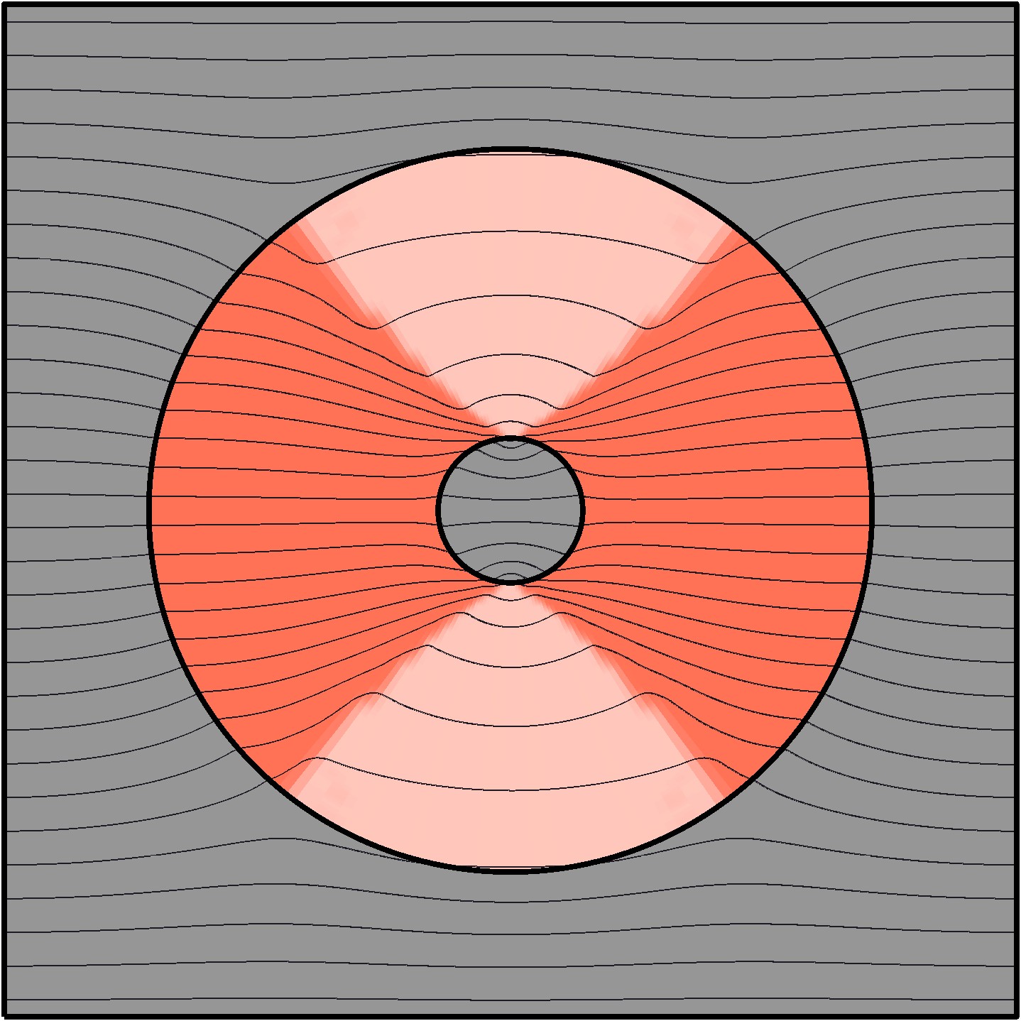
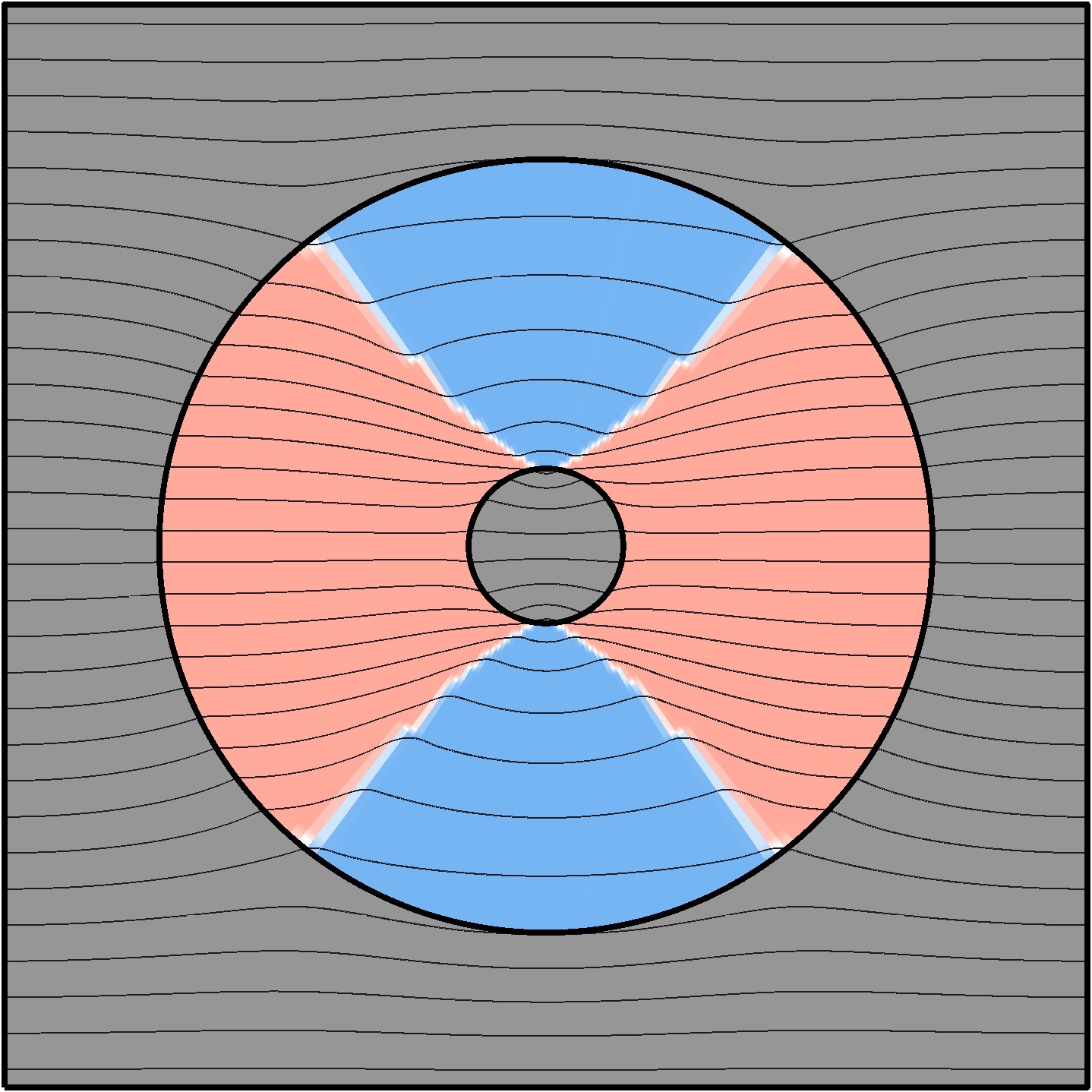
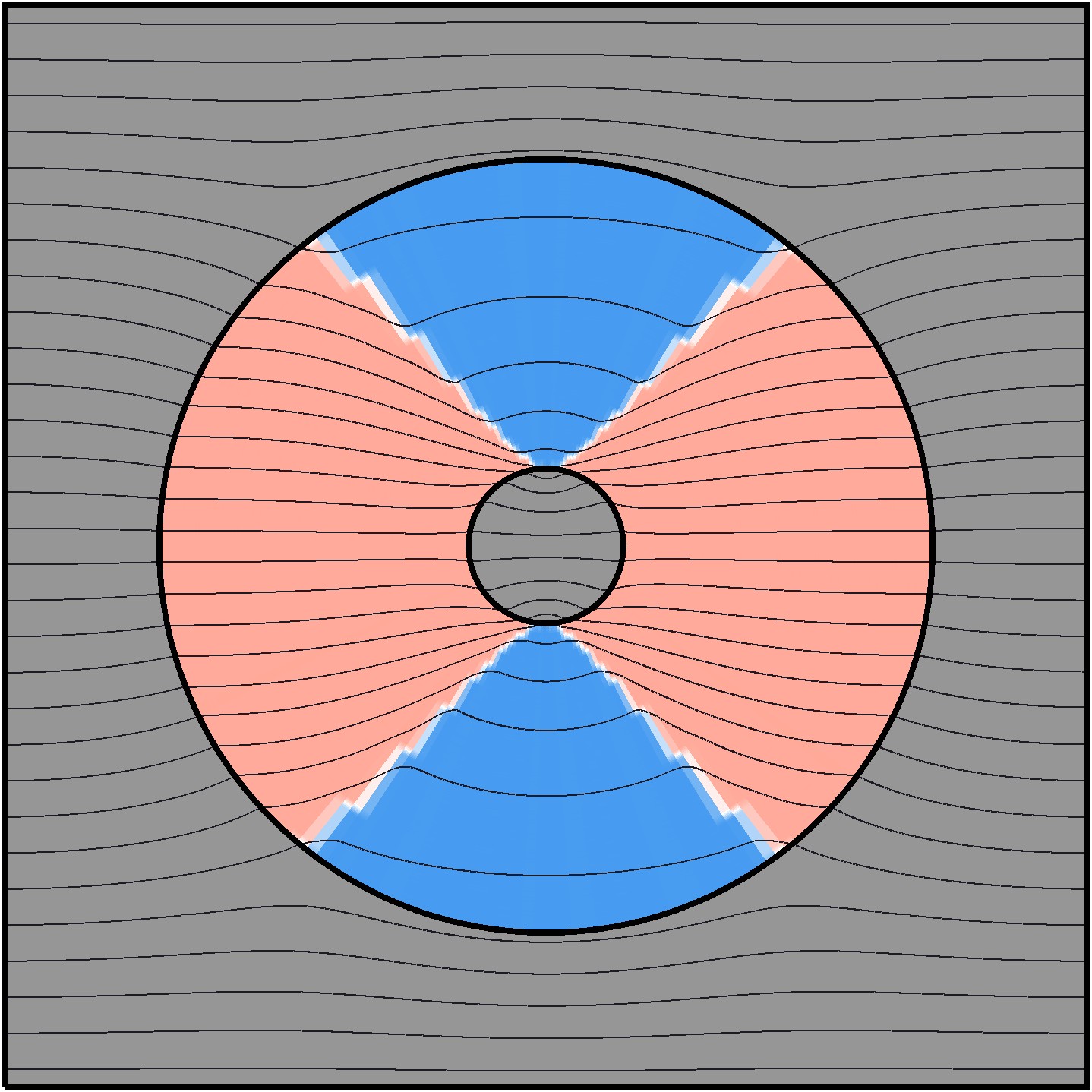
(g) $N_{\rm var}=1089$, $J=1.73\times 10^{-1}$, $\varPsi_{\rm cntr}=5.77$	(h) $N_{\rm var}=1089$, $J=1.86\times 10^{-1}$, $\varPsi_{\rm cntr}=5.39$	(i) $N_{\rm var}=1089$, $J=4.38\times 10^{-1}$, $\varPsi_{\rm cntr}=2.28$	(j) $N_{\rm var}=1089$, $J=3.01\times 10^{-1}$, $\varPsi_{\rm cntr}=3.32$	(k) $N_{\rm var}=1089$, $J=4.02\times 10^{-1}$, $\varPsi_{\rm cntr}=2.49$	(l) $N_{\rm var}=1089$, $J=3.36\times 10^{-1}$, $\varPsi_{\rm cntr}=2.97$

Figure 21: Optimized material distributions for the thermal concentrator problem. Six material models and $N_{\rm var}=25$, $1089$ are considered. Optimized concetrator function $\varPsi_{\rm cntr}$ values are from $2.12$ to $5.77$. All optimized material distributions are close to the sector-type geometry with alternative sectors of $\kappa_{\rm max}$-material and $\kappa_{\rm min}$-material. The intermediate densities/conductivities do not play much role in the design, and they are only present as the thinnest possible transition from $\kappa_{\rm min}$ to $\kappa_{\rm max}$ with the given design mesh.

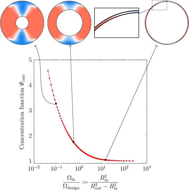
Figure 22: Change in the objective function $J_{\rm cntr}$ with respect to $\Omega_{\rm in}/\Omega_{\rm design}$. $R_{\rm in}$ is varied between $10$ mm to 49 mm, while keeping $R_{\rm out}=50$ mm constant. The optimized material distribution does not show any significant effect related to $R_{\rm in}$ increment, and maintains sector-type structure throughout.

Next, we design 2D thermal concentrators using all 6 material models and two design meshes with $N_{\rm var}=25$ and $1089$. The results are shown in Figure 6.1. We observe that the designed thermal concentrators can concentrate from 2.12 to 5.77 times more flux compared to a homogeneous plate. All optimized material distributions are close to the sector-type geometry with alternative sectors of $\kappa_{\rm max}$-material and $\kappa_{\rm min}$-material. The intermediate densities/conductivities do not play much role in the design, and they are only present as the thinnest possible transition from $\kappa_{\rm min}$ to $\kappa_{\rm max}$ with the given design mesh. Therefore, for a larger value of $N_{\rm var}$ such as $N_{\rm var}=1089$, the intermediate densities almost vanish before making the material distribution close to $\kappa_{\rm min}$-$\kappa_{\rm max}$ design.

Thermal concentrators made of sector-type geometries are already studied and experimentally demonstrated in Chen et.al. [99]. Our current results align well with the earlier results from Jansari et.al. [23], showcasing that the geometry with 4 sectors gives the best results. From both results, we can say that to concentrate more flux in $\Omega_{\rm in}$, the $\kappa_{\rm max}$ sectors need to widen their arc at $R_{\rm in}$ as well as $R_{\rm out}$. However, how much widening is feasible with the given configuration is dependent on the available thermal conductivities and the design freedom.

For all models with $N_{\rm var}=1089$, the arcs of $\kappa_{\rm max}$ sectors at $R_{\rm in}$ cover almost the entire perimeter, only leaving a very small length for $\kappa_{\rm min}$ sectors. One the other hand, the arcs of $\kappa_{\rm max}$ at $R_{\rm out}$ are almost similar for $N_{\rm var}=25$ & $N_{\rm var}=1089$. The curvature between $\kappa_{\rm min}$ & $\kappa_{\rm max}$ sectors also play an important part in guiding the extra flux towards $\Omega_{\rm in}$. For EMT and Maxwell models, the curvature is bigger compared to other models for $N_{\rm var}=1089$. This can mainly be attributed to the fact that the larger difference between $\kappa_{\rm min}$-$\kappa_{\rm max}$ allows to generate bigger curvature while maintaining the interface conditions. For other models, the curvature is constrained by a small difference between $\kappa_{\rm min}$ & $\kappa_{\rm max}$.

$v_{i}=0$	$v_{i}=0.25$	$v_{i}=0.5$	$v_{i}=0.75$	$v_{i}=1$
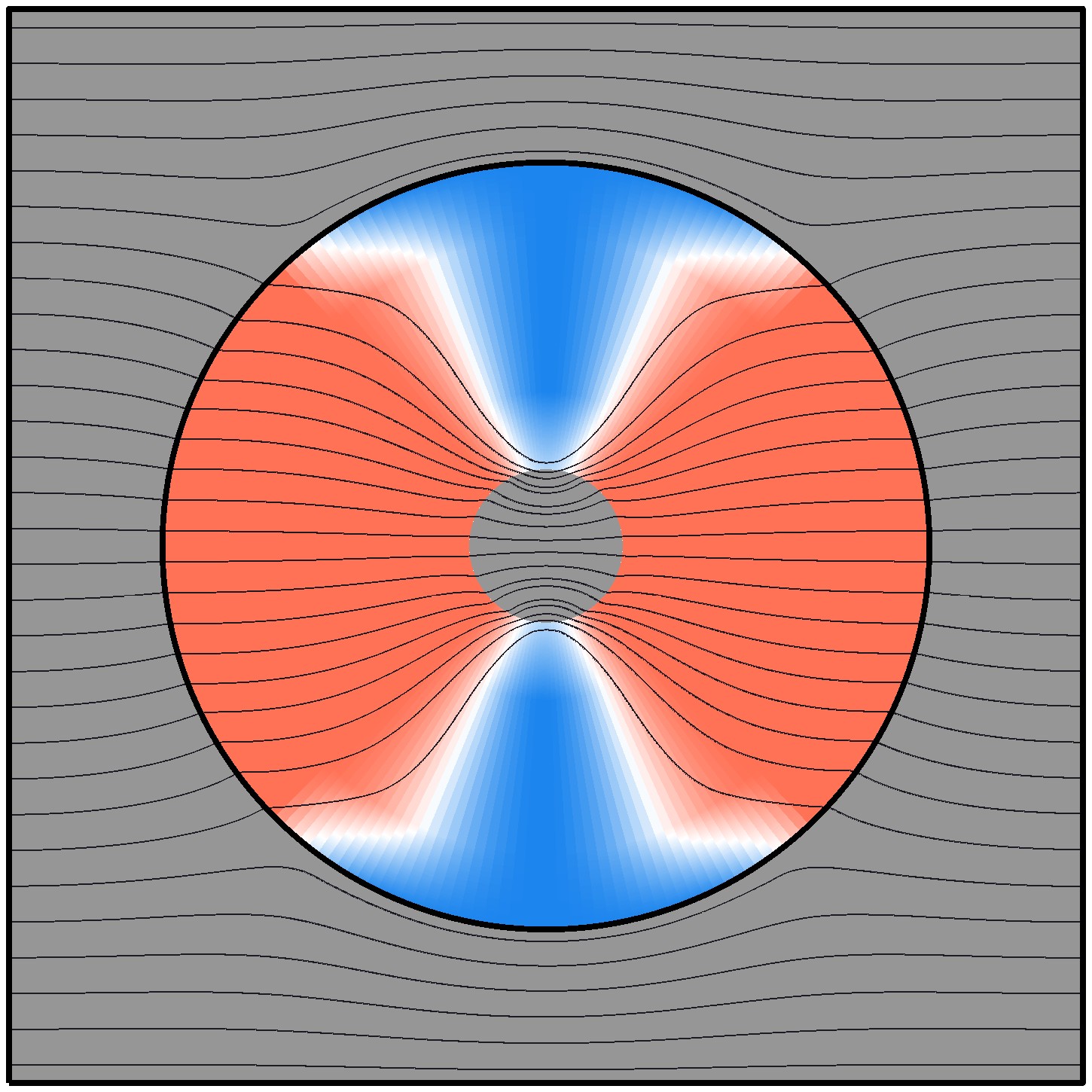
(a) $N_{\rm var}=25$, $J=2.19\times 10^{-1}$	(b) $N_{\rm var}=25$, $J=2.19\times 10^{-1}$	(c) $N_{\rm var}=25$, $J=2.19\times 10^{-1}$	(d) $N_{\rm var}=25$, $J=2.19\times 10^{-1}$	(e) $N_{\rm var}=25$, $J=2.19\times 10^{-1}$

Figure 23: Optimized material distributions for the thermal concentrator problem for $N_{\rm var}=25$ and EMT material model. Five different initial relative density distributions are considered with $v_{i}=0,0.25,0.5,0.75,1$, $i=1,2,...,N_{\rm var}$. All initial distributions reach the same solution with the objective function value $J=2.19\times 10^{-1}$.

Similar to the thermal cloak problem, we also study the effect of $\Omega_{\rm in}$/$\Omega_{\rm design}$ as well as different initial material distribution on optimized material distribution. For both studies, we consider $N_{\rm var}=25$ and EMT model. For the first study, we vary $R_{\rm in}$ between $10$ mm and 50 mm while maintaining $R_{\rm out}=50$ mm. Corresponding, optimized $\varPsi_{\rm cntr}$ are plotted in Figure 22. For the figure, we can say that the optimized material distribution does not show any significant effect related to $R_{\rm in}$ increment, and maintains sector-type structure throughout. For the second study, we take five initial distributions with $v_{i}=$ 0, 0.25, 0.5, 0.75, 1, $i=1,2,...,N_{\rm var}$. The optimization results are shown in Figure 23. All cases reach the same solution with $J=2.19\times 10^{-1}$ irrespective of their starting points. Results from both Figure 6.1 and Figure 23 exhibits the thermal concentrator problem has a lower degree of non-convexity than the thermal cloak problem.

In this paragraph, we present the result of 3D thermal concentrators designed with two material models (EMT and Gyroid) with $N_{\rm var}=129$. Figure 24 present the optimized material distributions for both cases, which can give concentration function value of $\varPsi_{\rm cntr}=11.36$ and $\varPsi_{\rm cntr}=3.47$. Analogous to the results of the 2D thermal concentrators, which yield sector-type material distributions, two spherical cones made of $\kappa_{\rm max}$-material are found along the $x$-axis. The remaining design domain is filled with $\kappa_{\rm min}$, leaving a very small transition region for intermediate densities. The flux concentration achieved using the thermal concentrator of the EMT model is presented in Figure 25.

EMT	Gyroid
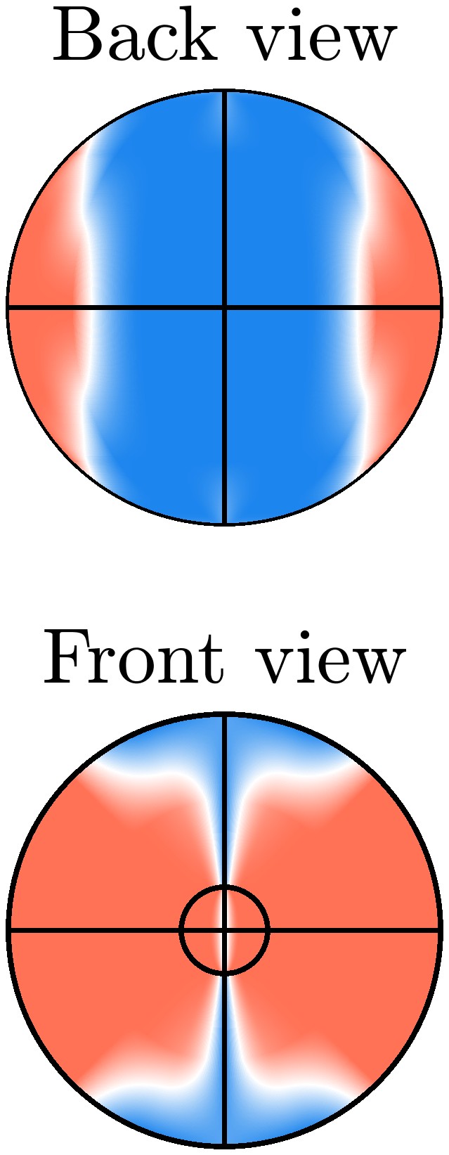
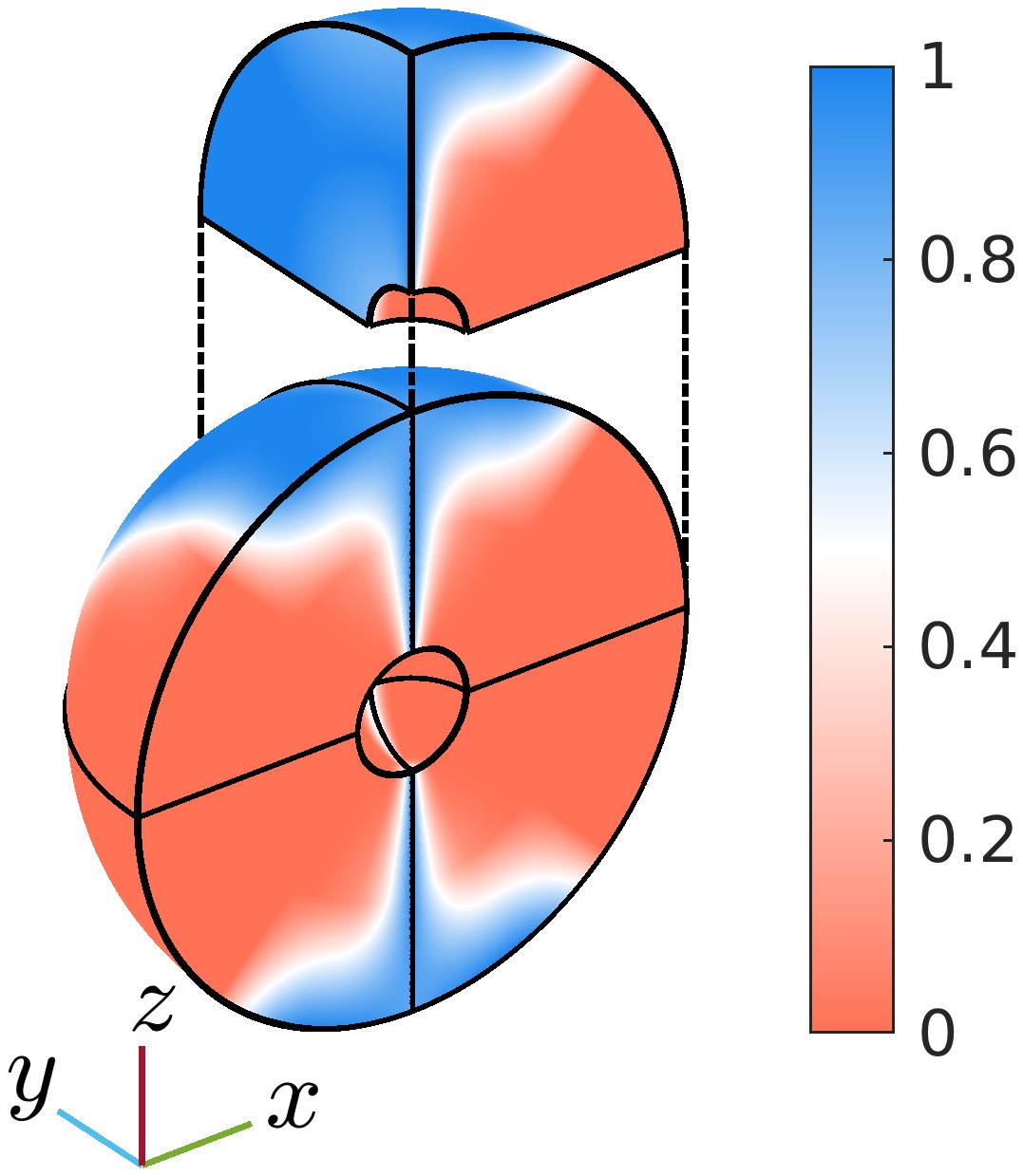
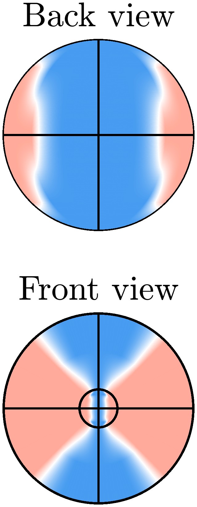
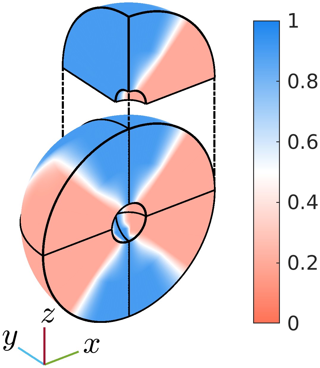
(a) $J_{\rm cntr}=8.81\times 10^{-2}$, $\varPsi_{\rm cntr}=11.36$	(b) $J_{\rm cntr}=2.88\times 10^{-1}$, $\varPsi_{\rm cntr}=3.47$

Figure 24: Optimized material distribution for the 3D thermal concentrators. Two material models (EMT and Gyroid) and $N_{\rm var}=129$ are explored. The proposed method could effectively design thermal concentrators concentrating 3 to 11 times more flux than a homogeneous plate. Analogous to the results of the 2D thermal concentrators, two spherical cones made of $\kappa_{\rm max}$-the material is found along the x-axis. The remaining design domain is filled with $\kappa_{\rm min}$, leaving a very small transition region for intermediate densities.

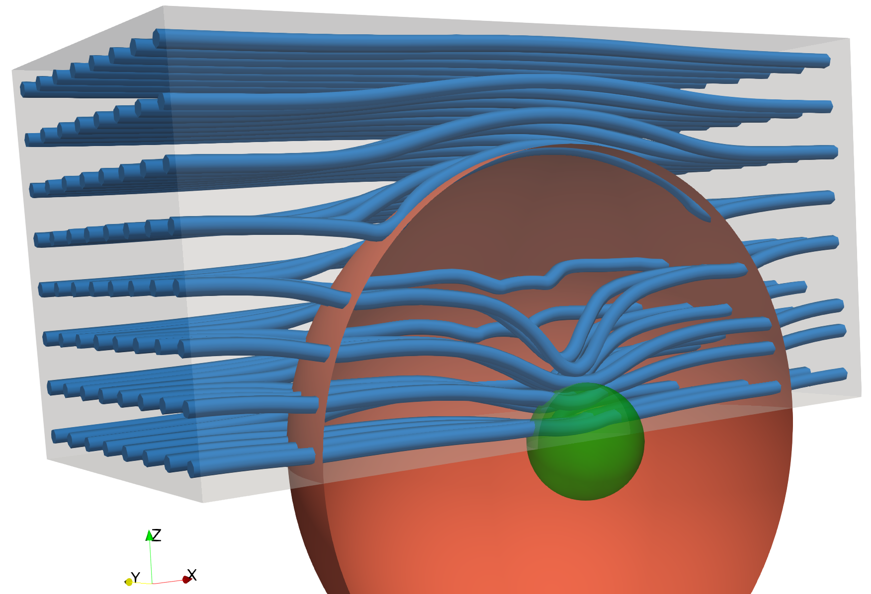
(a) Flux flow

(b) Optimized material distribution

Figure 25: Optimized material distribution and flux flow for the 3D thermal concentrators. EMT model and $N_{\rm var}=129$ are considered. Optimized objective function value $J_{\rm cntr}=8.81\times 10^{-2}$ and $\varPsi_{\rm cntr}=11.36$. The thermal concentrator guides the flux streamlines towards $\mathrm{\Omega}_{\mathrm{in}}$ to concentrate them.

6.2 Thermal rotator

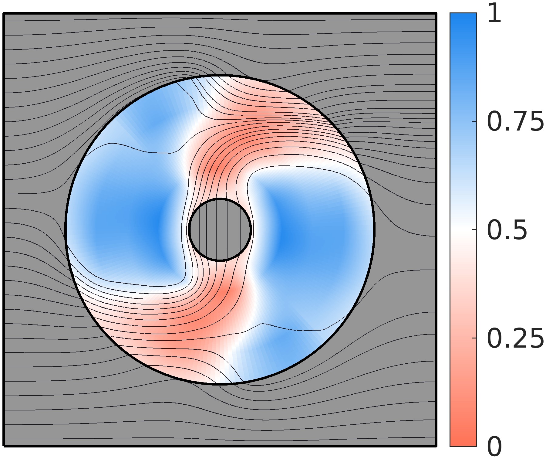
(a) $\theta=\nicefrac{{\pi}}{{2}}$, $J_{\rm rtr}=9.01\times 10^{-8}$

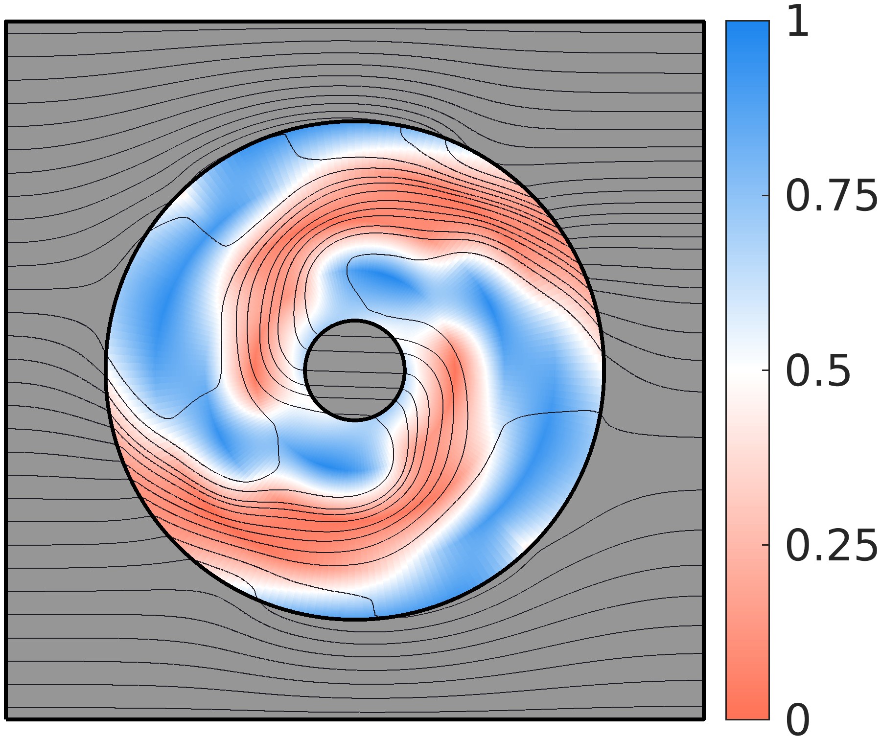
(b) $\theta={\pi}$, $J_{\rm rtr}=2.27\times 10^{-7}$

Figure 26: Optimized material distributions for the thermal rotator problem. EMT model, $N_{\rm var}=100$ and two values of $\theta$, $\theta=\nicefrac{{\pi}}{{2}},{\pi}$ are considered. Optimized objective function values are $J_{\rm rtr}=9.01\times 10^{-8}$ and $J_{\rm rtr}=2.27\times 10^{-7}$, respectively.

In this subsection, we design a 2D thermal rotator. The thermal rotator was first fabricated in [100] and later also designed for transient cases in [101] using transformation thermotics. The objective of a thermal rotator is to rotate the local direction of heat flux. In our case, we aim to rotate the flux passing through $\Omega_{\rm in}$. Accordingly, we design the objective function as:

$$J_{\mathrm{rtr}}=\dfrac{1}{\widetilde{J}_{\mathrm{rtr}}}\int_{\mathrm{\Omega}_{\mathrm{in}}}||~\mathbf{q}-\mathbf{R}~\overline{\mathbf{q}}~||^{2}~d\mathrm{\Omega},\quad\text{with}\quad\widetilde{J}_{\mathrm{rtr}}=\int_{\mathrm{\Omega}_{\mathrm{in}}}||~\overline{\mathbf{q}}~||^{2}~d\mathrm{\Omega}.$$ (36)

where $\mathbf{q}$ is the flux distribution, $\overline{\mathbf{q}}$ is the flux distribution when entire $\mathrm{\Omega}$ is filled with the base material, and $\mathbf{R}$ is a 2D rotation matrix defined as: $\mathbf{R}~=~\begin{bmatrix}\cos{\theta}&-\sin{\theta}\\ \sin{\theta}&\cos{\theta}\end{bmatrix}$, with $\theta$ being the angle of rotation.

Here, we take $R_{\rm in}=10$ mm, $R_{\rm out}=50$ mm, $L=140$ mm with base material filled in both $\Omega_{\rm in}$ and $\Omega_{\rm out}$. Considering the non-symmetry of the problem, we also removed the symmetry conditions for design variables. We have performed the optimization using $N_{\rm var}=100$ for two values of $\theta$, $\theta=\nicefrac{{\pi}}{{2}}$ and $\theta=\pi$. The optimized material distributions with the rotated flux in $\Omega_{\rm in}$ are shown in Figure 26.

6.3 Thermal cloaked sensor

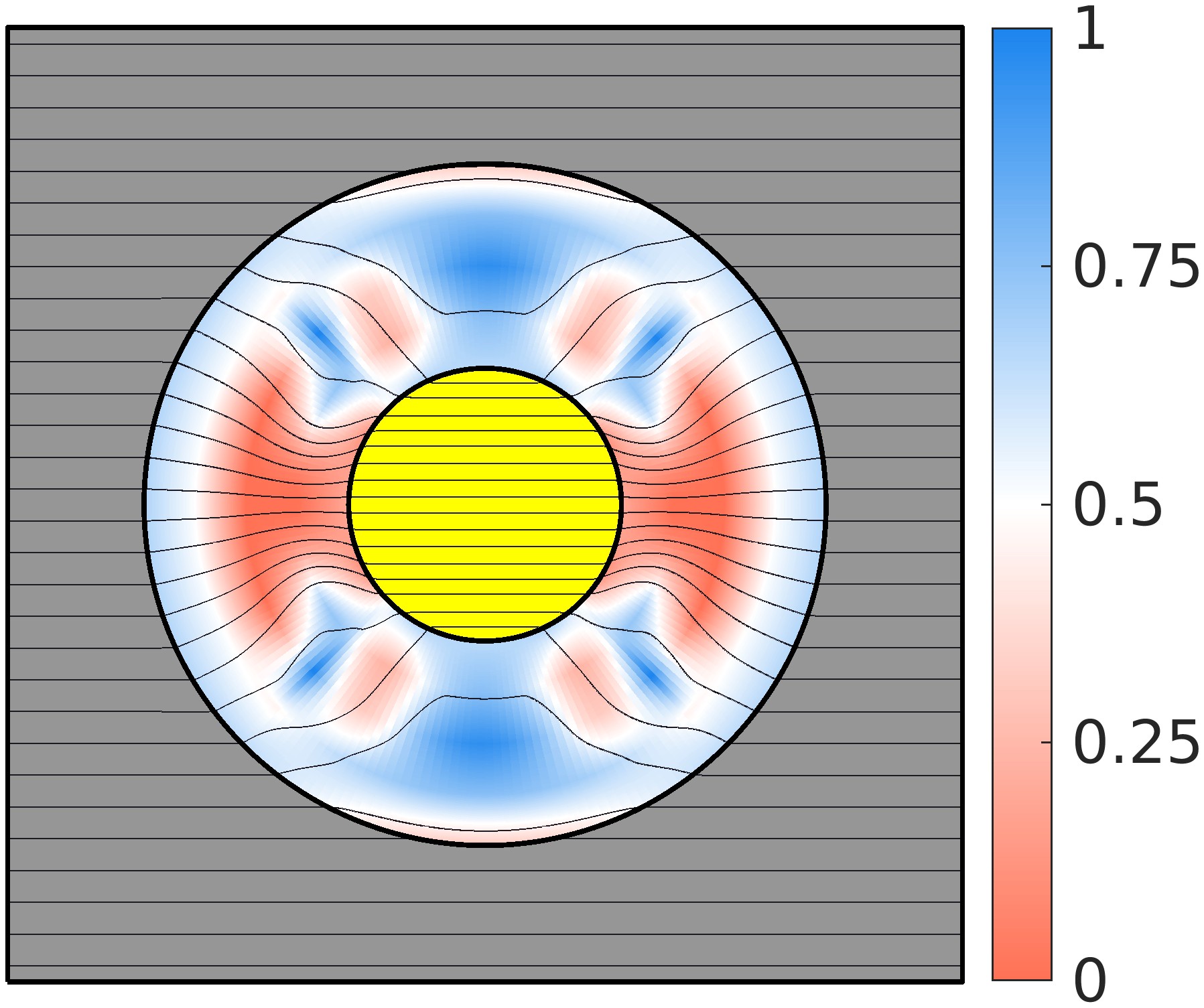
(a) Optimized material distribution

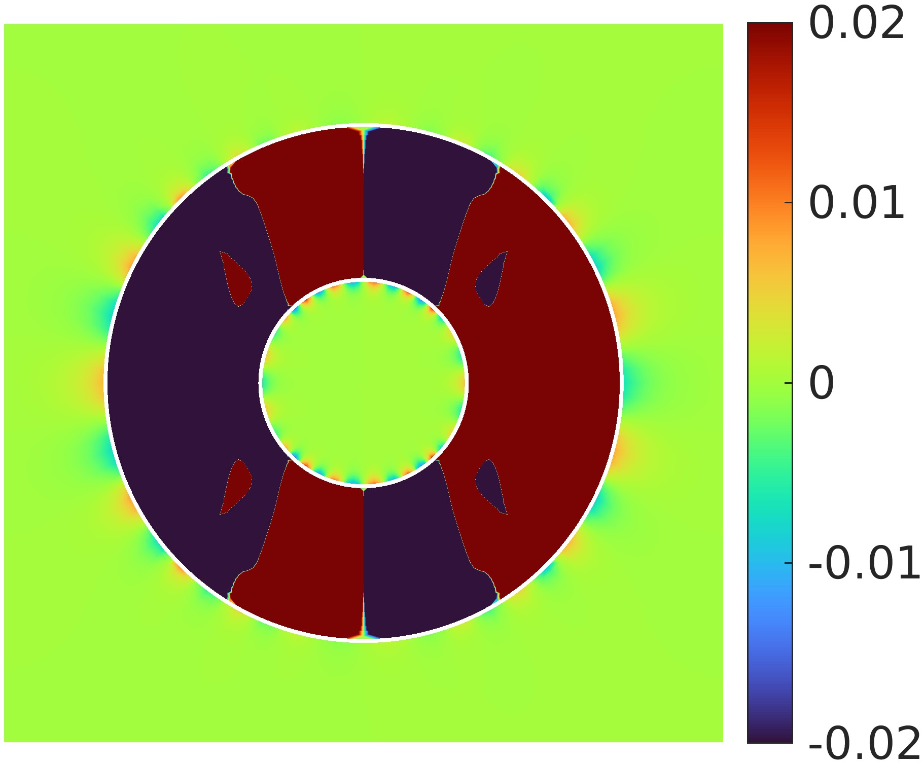
(b) Temperature difference $T-\overline{T}$

Figure 27: Optimized material distribution and temperature difference $T-\overline{T}$ for the thermal cloaked sensor problem. EMT model and $N_{\rm var}=25$ are considered. Optimized objective function value $J_{\rm cloaksen}=2.93\times 10^{-7}$. The thermal cloaked sensor keeps the flux streamlines horizontally undisturbed and diminishes the temperature disturbance in both $\mathrm{\Omega}_{\mathrm{in}}$ and $\mathrm{\Omega}_{\mathrm{out}}$.

Often, when a sensor is put in a physical field, the difference in properties between the background and sensor causes a disturbance around the sensor. This introduces undesirable noise in the measurement process. A thermal cloaked sensor tries to solve this issue by helping to generate the temperature profile as if the conductivities of the background and sensor are matching. As a result, the sensor has a thermal feeling of the background to measure and it can not be detected by the inline observation. Thermal cloaking sensors are already designed using other approaches in [102, 103, 104]. The objective function is defined as follows:

$$J_{\mathrm{cloaksen}}=\dfrac{1}{\widetilde{J}_{\mathrm{cloaksen}}}\int_{\mathrm{\Omega}_{\mathrm{in}}\cup\mathrm{\Omega}_{\mathrm{out}}}(T-\overline{T})^{2}~d\mathrm{\Omega},\quad\text{with}\quad\widetilde{J}_{\mathrm{cloaksen}}=\int_{\mathrm{\Omega}_{\mathrm{in}}\cup\mathrm{\Omega}_{\mathrm{out}}}(\widetilde{T}-\overline{T})^{2}~d\mathrm{\Omega},$$ (37)

where $\overline{T}$ is the temperature when entire $\mathrm{\Omega}$ is filled with the base material, $\widetilde{T}$ is the temperature when entire $\mathrm{\Omega}_{\rm design}\cup\mathrm{\Omega}_{\mathrm{out}}$ is filled with the base material.

Here, we take $R_{\rm in}=20$ mm, $R_{\rm out}=50$ mm, and $L=140$ mm. The base material is filled in $\Omega_{\rm out}$. $\Omega_{\rm in}$ represents an isotropic thermal sensor. We considered the thermal conductivity for sensor, $\kappa_{\rm sen}=130$ W/mK. The material distributions obtained by the optimization with $N_{\rm var}=25$ are shown in Figure 27. As the sensor has a higher conductivity than the base material, it needs more flux to create the same temperature profile as the base material. Therefore, the optimized material distribution has two sickle-shaped $\kappa_{\rm max}$-material structures along $x$-axis, which helps to concentrate more flux in $\Omega_{\rm in}$. Nevertheless, these structures remain unattached to the outer perimeter to prevent excessive streamline convergence, which could lead to temperature disturbances in $\Omega_{\rm out}$. Additionally, two dovetail-shaped $\kappa_{\rm min}$-material structures along the $y$-axis help to maintain the streamlines in a uniformly horizontal pattern inside $\Omega_{\rm in}$. We can see that the temperature difference in both $\Omega_{\rm in}$ and $\Omega_{\rm out}$ is negligible, with the objective function $J_{\rm cloaksen}=2.93\times 10^{-7}$.

6.4 Thermal cloak-concentrator

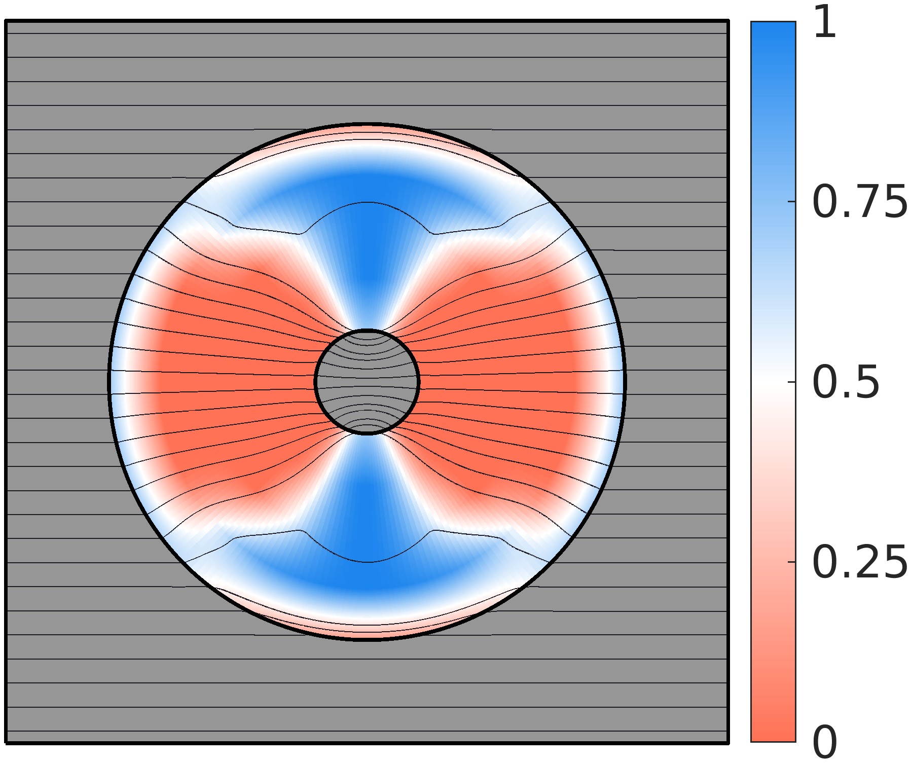
(a) Optimized material distribution

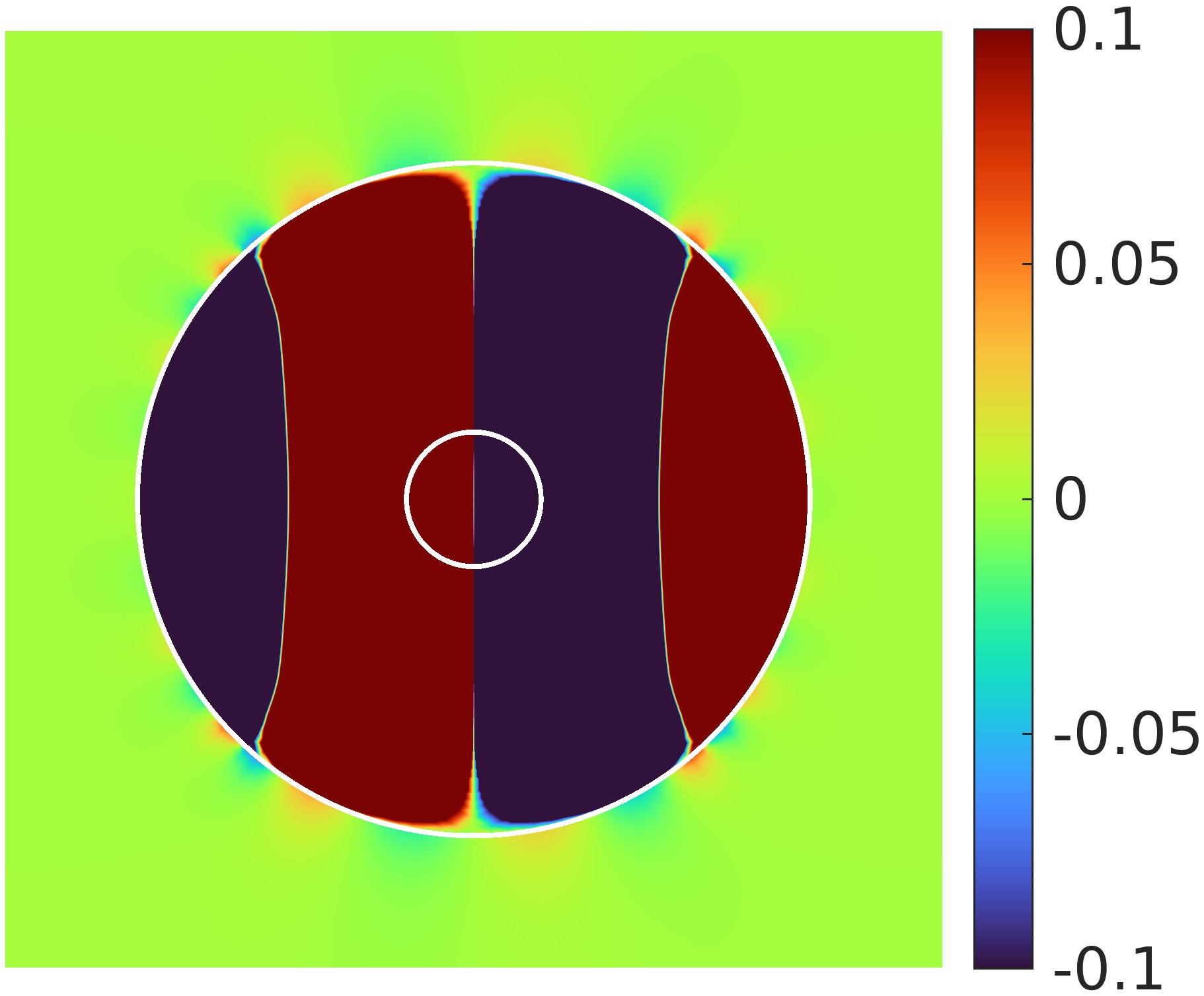
(b) Temperature difference $T-\overline{T}$

Figure 28: Optimized material distribution and temperature difference $T-\overline{T}$ for the thermal cloak-concentrator problem. EMT model and $N_{\rm var}=25$ are considered. Optimized objective function value $J_{\rm cloakcntr}=8.21\times 10^{-3}$ with $J_{\rm cloak}=2.97\times 10^{-4}$ & $\varPsi_{\rm cntr}=3.35$. The thermal cloak-concentrator effectively achieves dual functionality—cloaking and concentrating— by balancing on each function.

In this manipulator we designed a multi-functional thermal meta-structure. The cloak-concentrator performs the combined task of concentrating the flux in $\Omega_{\rm in}$ and cloaking $\Omega_{\rm in}$ as well. Thermal cloak-concentrators are constructed in articles [105, 106, 23] using other methods. The total objective function is defined as follows:

$$J_{\mathrm{cloakcntr}}=J_{\mathrm{cloak}}+\dfrac{1}{\varPsi_{\rm cntr}^{4}}.$$ (38)

where $J_{\mathrm{cloak}}$ & $\varPsi_{\rm cntr}$ are functions for cloaking and concentrating as defined in Eqs. (31) -(35).

Here, we take $R_{\rm in}=10$ mm, $R_{\rm out}=50$ mm, and $L=140$ mm. The base material is filled in both $\Omega_{\rm in}$ and $\Omega_{\rm out}$. The optimization tries to find the balance between both objectives according to their relative weightage as given in Eq. (38). The material distribution obtained by the optimization with $N_{\rm var}=25$ is shown in Figure 28. Corresponding total objective function $J_{\rm cloakcntr}=6.35\times 10^{-3}$ with $J_{\rm cloak}=6.12\times 10^{-4}$ and $\varPsi_{\rm cntr}=3.63$. The optimized material distribution resembles one with a concentrator. However, the conductivities near $R_{\rm out}$ in $\Omega_{\rm design}$ vary to accommodate the cloaking function. These conductivities must be adjusted to ensure that the streamlines do not converge prematurely in $\Omega_{\rm out}$ just before entering $\Omega_{\rm design}$.

6.5 Thermal horizontal concentrator-vertical cloak

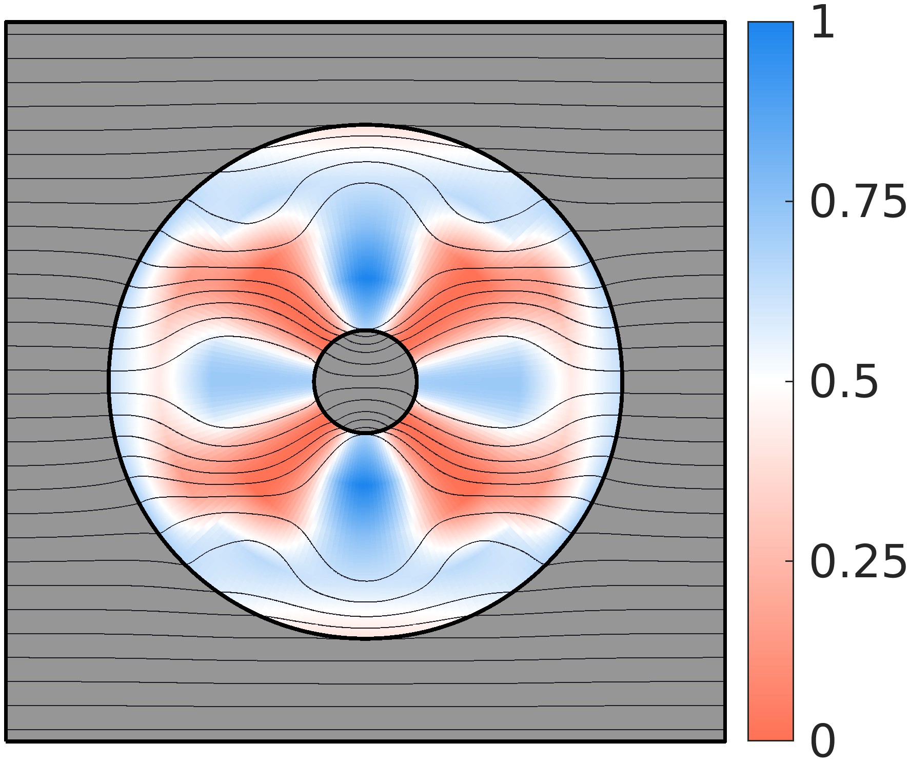
(a) Optimized material distribution and flux flow for the horizontal applied flux

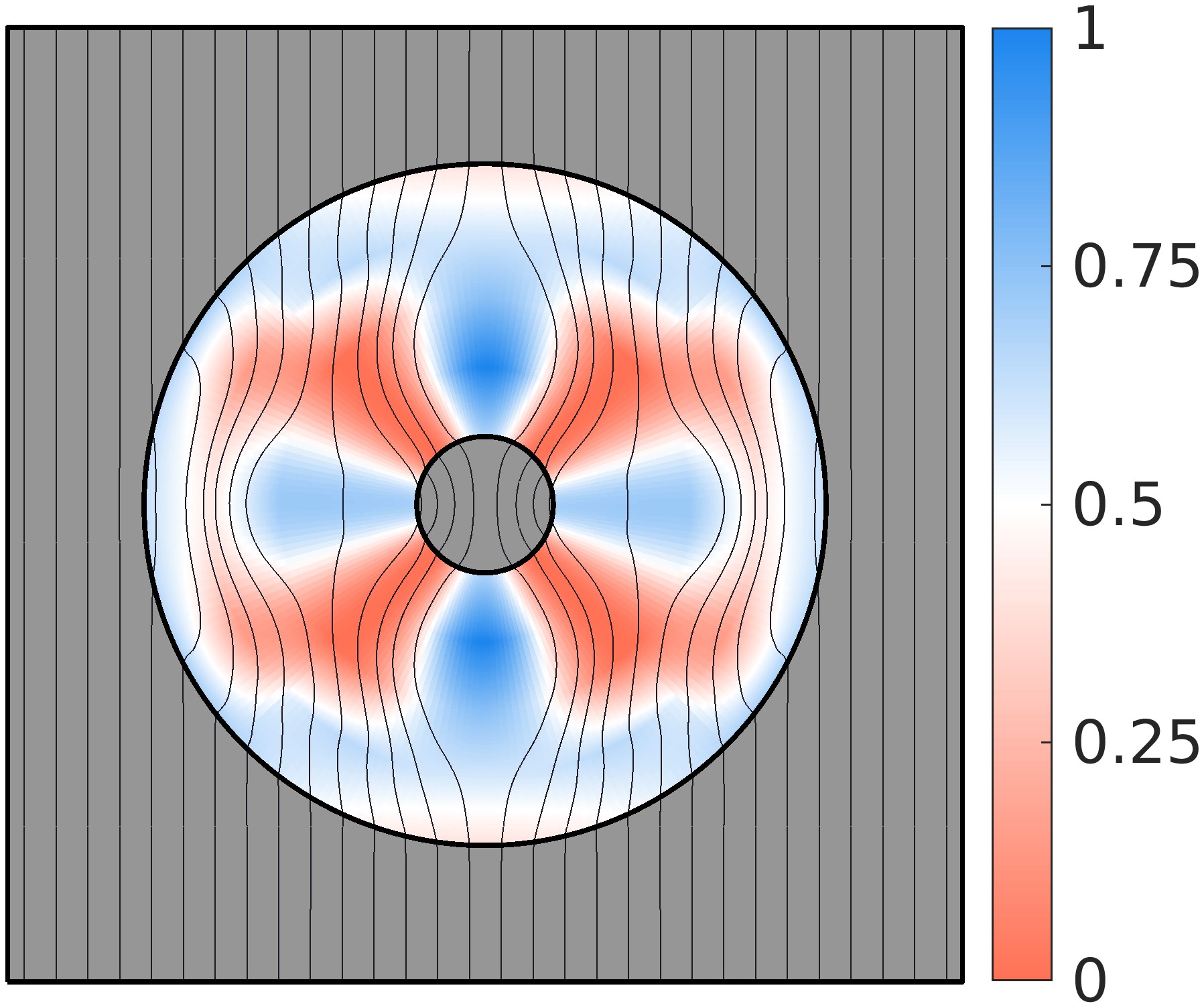
(b) Optimized material distribution and flux flow for the vertical applied flux

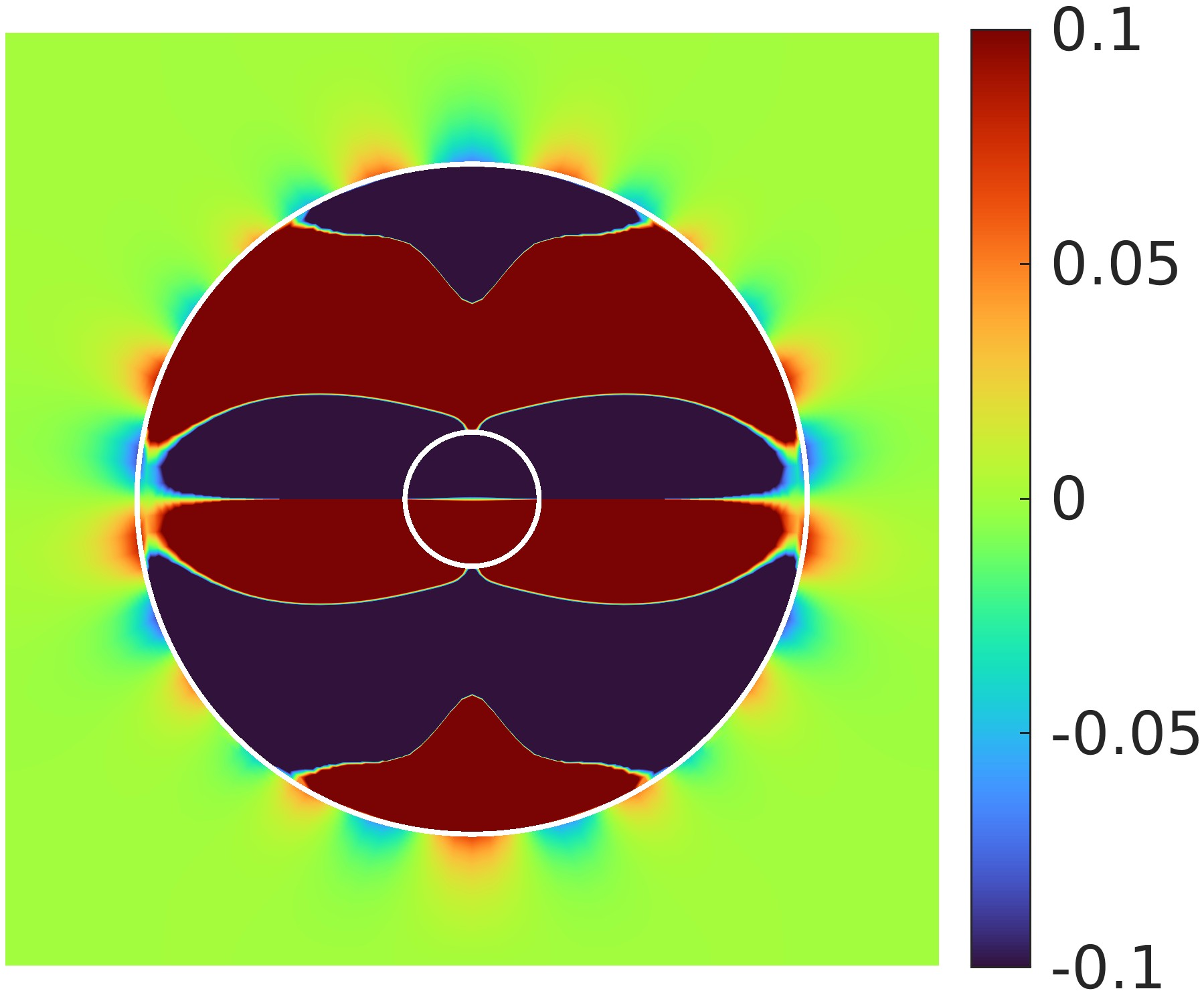
(c) Temperature difference $T-\overline{T}$

Figure 29: Optimized material distribution (for the horizontal applied flux); optimized material distribution and temperature difference $T-\overline{T}$ (for the vertical applied flux) for thermal bi-directional thermal meta-structure (horizontal concentrator and vertical cloak). EMT model and $N_{\rm var}=25$ are considered. Optimized objective function value $J_{\rm cloakcntr}=1.75\times 10^{-2}$ with $J_{\rm cloak}=1.31\times 10^{-3}$ & $\varPsi_{\rm cntr}=2.80$.

In this subsection, we design a bi-directional thermal meta-structure, which behaves as two different thermal meta-structures under two different sets of boundary conditions. Here, we aspire to design a thermal meta-structure that works as a concentrator for applied horizontal constant temperature difference while as a cloak for applied horizontal constant temperature difference. We use the objective function defined earlier in Eq. (38), however, $J_{\mathrm{cloak}}$ & $\varPsi_{\mathrm{cntr}}$ are calculated on two different temperature distributions based on two different sets of boundary conditions. For the cloak, we consider standard $300$ K constant temperature on the left side and $200$ K temperature on the right side, while for the concentrator the same conditions are applied on the top and bottom sides, respectively. For both cases, the remaining sides are considered as adiabatic walls. All dimensions and material allocation are the same as described in Section 6.4. The material distribution obtained by the optimization with $N_{\rm var}=25$ is shown in Figure 29. Optimized material distribution can achieve the objective function value $J_{\rm cloakcntr}=1.75\times 10^{-2}$ with cloaking function $J_{\rm cloak}=1.31\times 10^{-3}$ and concentrating function $\varPsi_{\rm cntr}=2.80$.

7 Reconstruction of Architected Cellular Materials (ACMs)

From the results of the optimization of ACMs, we can reconstruct the entire structures using the density distribution and predefined unit-cells (Gyroid and TCOH in our case). We have shown here a primary reconstructed (thin-walled) Gyroid-based structure, without any manufacturing or design constraints. Note that the results obtained from the optimization provide the density field of porosity in terms of NURBS surface. Based on this surface, the density at any point on the domain can be calculated by the method of projection.

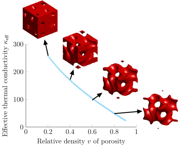
Figure 30: The relation between effective thermal conductivity and relative density $v$ of porosity. Four thin-walled Gyroid unit-cells corresponding to $v=0.2,0.4,0.6,0.8$ are also shown.

The unit-cell of thin-walled Gyroid is defined implicitly using Boolean operation. The volume is the intersection volume between two implicit surfaces given by:

$$\cos{\left(\dfrac{2\pi}{a}x\right)}\sin{\left(\dfrac{2\pi}{a}y\right)}+\cos{\left(\dfrac{2\pi}{a}y\right)}\sin{\left(\dfrac{2\pi}{a}z\right)}+\cos{\left(\dfrac{2\pi}{a}z\right)}\sin{\left(\dfrac{2\pi}{a}x\right)}\pm t=0,$$ (39)

where $a$ is the side length of a cubic unit-cell and $t$ is the control parameter ($2t$ will be the thickness of the wall). The approximate relation between the relative density $v$ of porosity and control parameter $t$ is given as [107]:

$$t=\dfrac{0.65}{v_{m}}\quad\text{with}\quad v_{m}=1-v,$$ (40)

where $v_{m}$ and $v$ are densities of matrix material and porosity, respectively. The relation between thermal conductivity and Gyroid shape is also plotted in Figure 30.

ACMs are constructed by tessellating a repeating unit-cell, across the domain. There are several techniques to tessellate the unit-cell such as sweeping, meshing and trimming [108]. In the swept ACMs, alignment with the boundary of the domain is enforced and this type of structure highly depends on the curvature of the boundary. Therefore, unit-cells deviate from their original shapes and properties. In the meshed ACMs, the unit-cells are mapped to the elements of the domain mesh. This mesh could be a finite element mesh used for the numerical analysis. Similar to the swept ACMs, the elements and the corresponding unit-cells follow the external geometry. Eventually, the unit-cells of the meshed ACMs deviate from their original properties too. On the contrary, the tessellation based on the trimming approach does not carry this limitation and mostly retains the properties of unit-cells. It can effectively create a complex-shaped ACM with the simple Boolean operations of the domain and tessellated unit-cells. In our case, we use the trimming approach considering our design geometries involve circular and spherical shapes. Trimmed ACMs often possess weak boundaries which lack support. A potential remedy is to create a solid skin surrounding the lattice structure [108]. However, as our design domain is always surrounded by other homogeneous materials, we do not need any specific treatment for support.

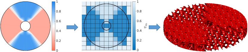
Figure 31: Reconstruction of a Gyroid-based thermal concentrator obtained by topology optimization. A very coarse $11\times 11$ voxel mesh is considered to highlight the gradation and reconstruction features.

For the reconstruction, we consider a rectangular (cubical) background domain that entirely covers our actual 2D (3D) domain. Then, the background domain is voxelized, which essentially means discretizing the geometry in small rectangular (cubical) blocks [108]. It is assumed that one voxel corresponds to one unit-cell and its density is calculated at the center of the voxel. The voxels that entirely outside the domain will be considered empty and given $v_{m}=0$, while the densities at the center of the remaining voxels will be calculated based on the NURBS entity describing the density distribution. There might be a possibility that the center of any voxel cut on the boundary might lie outside the design domain. In that case, the density value is calculated on the basis of the extrapolation of the density surface. Then, the control parameter $t$ and the corresponding Gyroid are constructed for all voxels using Eqs. (40)-(39). When all unit-cells are put together in the voxelized domain, it is referred to as the unit-cell tessellation. Finally, a Boolean intersection operation is performed between the actual domain and unit-cell tessellation to find the final trimmed ACM. The reconstruction steps are explained for a thermal concentrator in Figure 31. We consider a coarse voxel mesh to highlight the characteristics of the reconstruction process. However, in actual structures, a finer mesh is required so that the scale separation hypothesis is satisfied [87]. By satisfying the scale separation hypothesis, we ensure that the homogenization rule and eventually the optimization results remain valid. A full-scale reconstructed 2D thermal concentrator and a 2D complex star-shaped thermal cloak based on a very fine voxel mesh are shown in Figure 32.

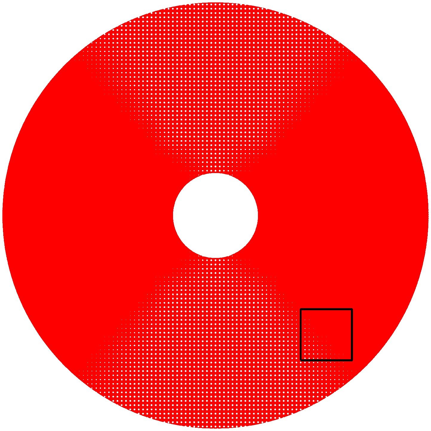
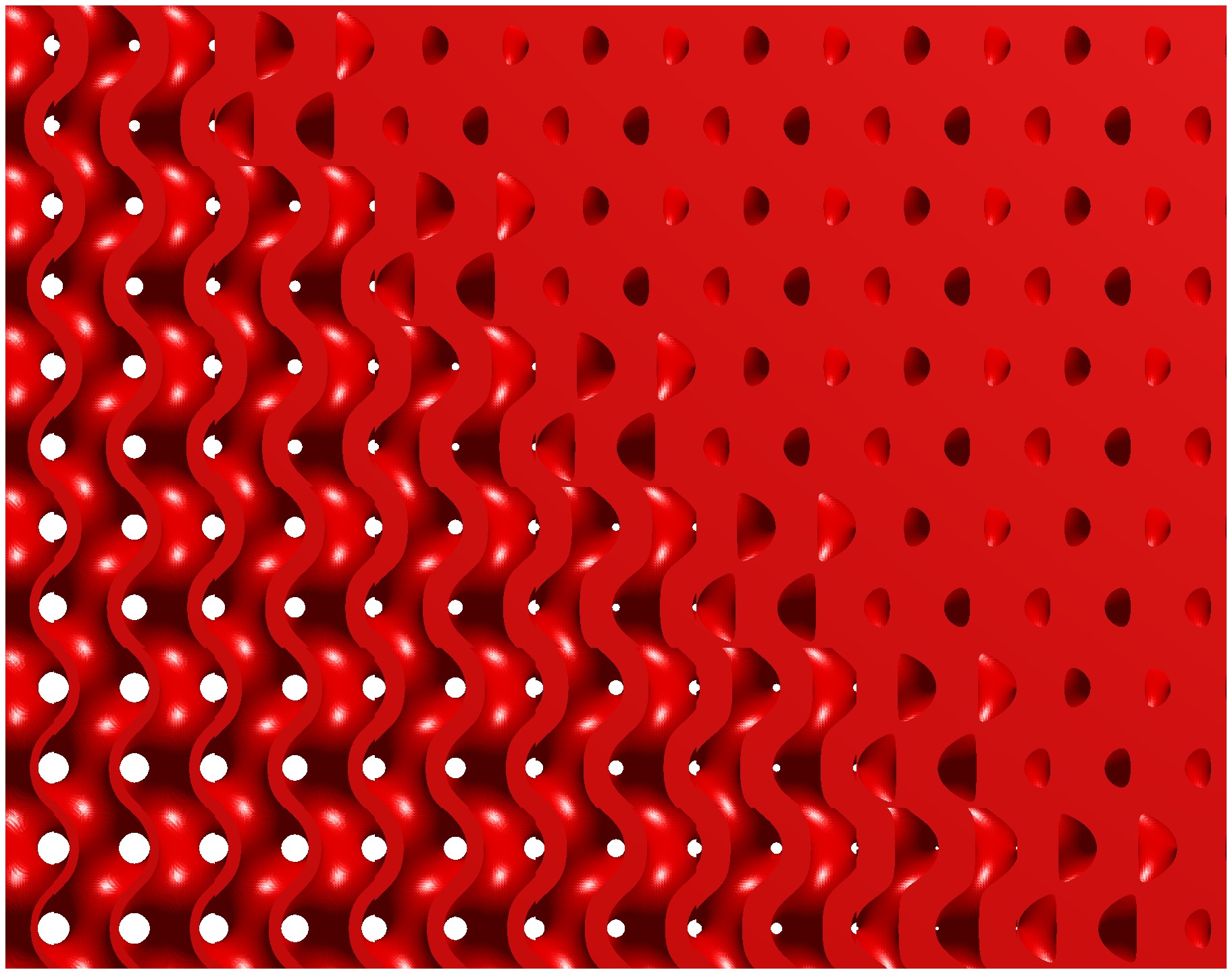
(a) 2D thermal concentrator

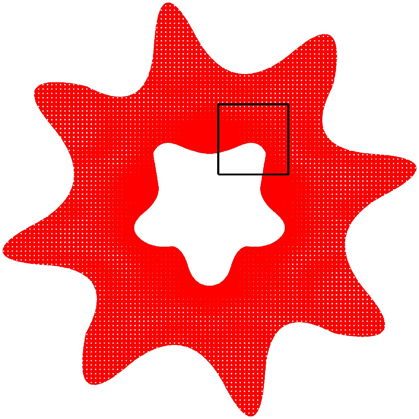
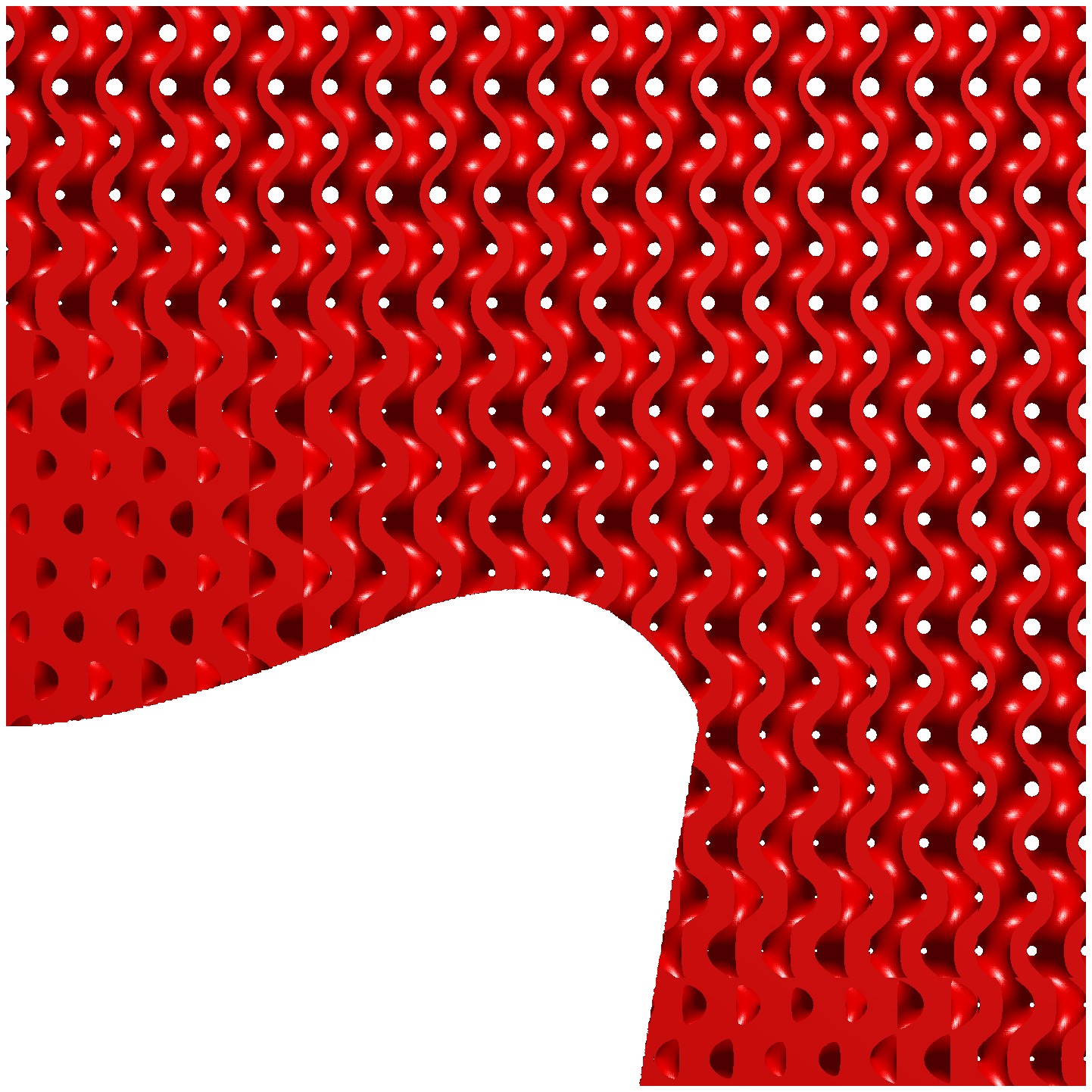
(b) 2D complex star-shaped thermal cloak

Figure 32: Full-scale reconstruction of thermal meta-structures.

8 Conclusions

In this paper, we proposed FGM-based thermal metamaterials/meta-structures. We used the isogeometric density topology optimization method to design these meta-structures, in which the density, geometry, and solution fields are parameterized using NURBS basis functions. Following the NURBS parameterizations, IGA is utilized to solve boundary value problems. IGA gives an accurate geometric description and ease in handling higher smoothness and inter-element continuity. Additionally, NURBS-parameterized density field has a few perks in comparison to element or nodal densities, including smoother material distributions, inherent filtering against checker-boarding and straightforward calculation of the gradient of the density field.

We showcase the versatility of the proposed method by designing various 2D and 3D thermal meta-structures including thermal cloaks, thermal concentrators, thermal rotators and thermal cloaked sensors. The method is robust in handling diverse material models, geometries, boundary conditions and design requirements. It can also produce alternate designs for non-convex problem by slight modification in optimization parameters or initial designs. This versatility, robustness and flexibility is one of the key benefits of our proposed tool over conventional methods (which mainly function under limited design scenarios due to their analytical nature). Additionally, the proposed method does not need any intuition-based case-dependant information. We also showed that the method can effectively design thermal meta-structures made of architected cellular materials. In order to do so, the numerical homogenization data of their unit-cells are implemented as the material law in the formulation. In the end, the full structure is generated based on the obtained density distribution and density-control parameter relation of the unit-cell.

Acknowledgements

We are grateful for the support of the University of Luxembourg. The calculations presented in this paper were carried out using the HPC facilities of the University of Luxembourg.

Appendix A Matrix formulation of boundary value problem

The global stiffness matrix $\mathbf{K}$ and the global flux vector $\mathbf{F}$ (as shown in Eq. (6)) are written as:

$$\mathbf{K}=\mathbf{K}^{b}+\mathbf{K}^{n}+(\mathbf{K}^{n})^{\rm T}+\mathbf{K}^{s}+\mathbf{K}^{r},$$ (41)

$$\mathbf{F}=\sum_{k\in{\rm\{in,design,out\}}}\int_{\Omega_{k}}(\mathbf{N}^{k})^{\textrm{T}}q_{b}~d\Omega+\int_{\Gamma_{N}}\mathbf{N}^{\textrm{T}}q_{n}~d\Gamma+\int_{\Gamma_{R}}\mathbf{N}^{\textrm{T}}hT_{\infty}~d\Gamma,$$ (42)

where $\mathbf{K}^{b}$ is the bulk stiffness matrix; $\mathbf{K}^{n}$ and $\mathbf{K}^{s}$ are the interfacial stiffness matrices; and $\mathbf{K}^{r}$ is the convective flux matrix (related to the robin boundary conditions). As $\Omega_{\rm in}$, $\Omega_{\rm out}$ and $\Omega_{\rm design}$ are considered separate NURBS patches, $\mathbf{K}^{b}$, $\mathbf{K}^{n}$ and $\mathbf{K}^{s}$ are defined as follows (following the notations used in Section 2),

$$\mathbf{K}^{b}=\sum_{k\in{\rm\{in,design,out\}}}\int_{\Omega_{k}}(\mathbf{B}^{k})^{\textrm{T}}\bm{\kappa}^{k}(v)\mathbf{B}^{k}~d\Omega,$$ (43)

$$\mathbf{K}^{n}=\begin{bmatrix}-\gamma\displaystyle\int_{\Gamma_{I}}(\mathbf{N}^{1})^{\textrm{T}}\bm{n}\bm{\kappa}^{1}(v)\mathbf{B}^{1}~d\Gamma&-(1-\gamma)\displaystyle\int_{\Gamma_{I}}(\mathbf{N}^{1})^{\textrm{T}}\bm{n}\bm{\kappa}^{2}(v)\mathbf{B}^{2}~d\Gamma\\[1.00006pt] \gamma\displaystyle\int_{\Gamma_{I}}(\mathbf{N}^{2})^{\textrm{T}}\bm{n}\bm{\kappa}^{1}(v)\mathbf{B}^{1}~d\Gamma&(1-\gamma)\displaystyle\int_{\Gamma_{I}}(\mathbf{N}^{2})^{\textrm{T}}\bm{n}\bm{\kappa}^{2}(v)\mathbf{B}^{2}~d\Gamma\end{bmatrix},$$ (44)

$$\mathbf{K}^{s}=\begin{bmatrix}\beta\displaystyle\int_{\Gamma_{I}}(\mathbf{N}^{1})^{\textrm{T}}\mathbf{N}^{1}~d\Gamma&-\beta\displaystyle\int_{\Gamma_{I}}(\mathbf{N}^{1})^{\textrm{T}}\mathbf{N}^{2}~d\Gamma\\[1.00006pt] -\beta\displaystyle\int_{\Gamma_{I}}(\mathbf{N}^{2})^{\textrm{T}}\mathbf{N}^{1}~d\Gamma&\beta\displaystyle\int_{\Gamma_{I}}(\mathbf{N}^{2})^{\textrm{T}}\mathbf{N}^{2}~d\Gamma\end{bmatrix},$$ (45)

$$\mathbf{K}^{r}=\int_{\Gamma_{R}}h(\mathbf{N})^{\textrm{T}}~\mathbf{N}~d\Omega,$$ (46)

where $\mathbf{B}$ is the matrix of basis function derivatives and $\mathbf{N}$ is the vector of basis functions.

In Section 4.3, the derivative of global stiffness matrix $\mathbf{K}$ with respect to relative density $v$ will be needed in the sensitivity calculation. It is defined by differentiating Eq. (41) as follows:

$$\dfrac{d\mathbf{K}}{dv}=\dfrac{d\mathbf{K}^{b}}{dv}+\dfrac{d\mathbf{K}^{n}}{dv}+\left(\dfrac{d\mathbf{K}^{n}}{dv}\right)^{\rm T}+\dfrac{d\mathbf{K}^{s}}{dv},$$ (47)

where

$$\dfrac{d\mathbf{K}^{b}}{dv}=\sum_{k\in{\rm\{in,design,out\}}}\int_{\Omega_{k}}(\mathbf{B}^{k})^{\textrm{T}}\dfrac{d\bm{\kappa}^{k}(v)}{dv}\mathbf{B}^{k}~d\Omega,$$ (48)

and $\dfrac{d\mathbf{K}^{n}}{dv}$ & $\dfrac{d\mathbf{K}^{s}}{dv}$ are defined similarly by differentiating Eq. (44) & Eq. (45), respectively.

Appendix B Mesh sensitivity analysis

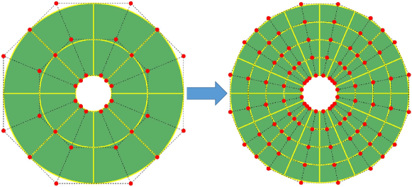
Figure 1: The solution mesh refinement strategy using the knot insertion procedure. At each stage, new knots are added at midpoints of existing knot spans in each parametric direction.

At first, we conducted a mesh sensitivity analysis to find a sufficiently fine solution mesh for a given design mesh to ensure an adequate level of solution accuracy. A mesh model of a 2D NURBS patch is shown in Figure 1. We consider two design meshes with $N_{\rm var}=25$ & $N_{\rm var}=81$. For both meshes, we run the optimization problems with several stages of refinements for the solution mesh, starting with the same number of control points in the solution and design meshes. For each refinement, we insert new knots at midpoints of existing knot spans in each parametric direction as shown in Figure 1. For $N_{\rm var}=25$ & $N_{\rm var}=81$, we perform 5 and 4 stages of refinements, respectively. The last refinement solution is considered as the reference solution to calculate the relative error.

We perform the mesh sensitivity analysis for the 2D thermal cloak and 2D thermal concentrator. The relative error in the relative density field $v$ over $\Omega_{\rm design}$ with respect to number of degrees of freedom (DOF) is shown in Figure 2. We consider $2\%$ error as an acceptable error, which is represented by a black horizontal line in the figure. We observe that, for thermal cloak, all solution meshes and, for thermal concentrator, the solution meshes with DOF$>10^{4}$ satisfy the criterion. Therefore, we take a mesh with DOF=13167 as the solution mesh for both cases.

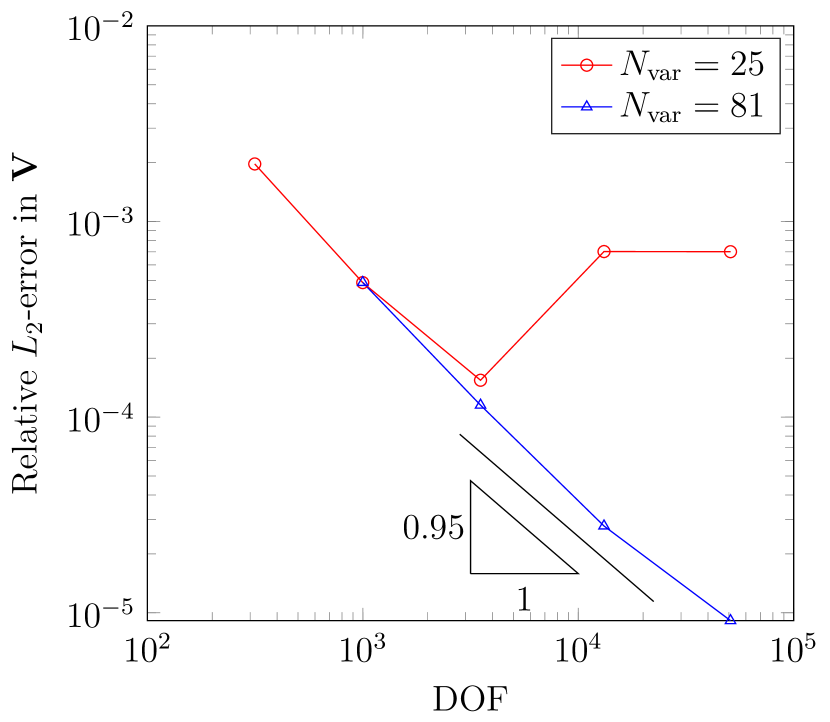
(a) 2D thermal cloak

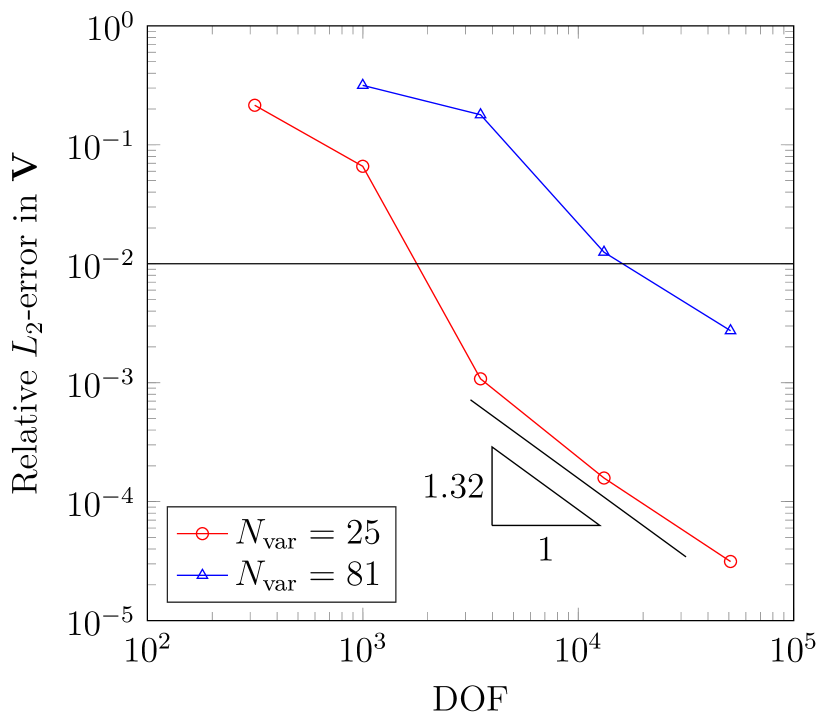
(b) 2D thermal concentrator

Figure 2: Relative error in volume fraction $v$ value over $\Omega_{\rm design}$ with respect to the number of degrees of freedom of solution mesh for (a) 2D thermal cloak problem and (b) 2D thermal concentrator problem. The last refinement solution is considered as the reference solution to calculate the relative error. We consider $2\%$ relative error as an acceptable error, which is represented by the black horizontal line.

Data availability

Data will be made available on request.

References

- Yang et al. [2021] S. Yang, J. Wang, G. Dai, F. Yang, J. Huang, Controlling macroscopic heat transfer with thermal metamaterials: Theory, experiment and application, Physics Reports 908 (2021) 1–65.
- Dai [2021] G. Dai, Designing nonlinear thermal devices and metamaterials under the Fourier’s law: A route to nonlinear thermotics, Frontiers of Physics 16 (2021) 53301. ArXiv:2103.13305 [physics].
- Kadic et al. [2013] M. Kadic, T. Bückmann, R. Schittny, M. Wegener, Metamaterials beyond electromagnetism, Reports on Progress in Physics 76 (2013) 126501. 311 citations (Crossref) [2023-01-19].
- Peralta et al. [2020] I. Peralta, V. D. Fachinotti, J. C. Álvarez Hostos, A Brief Review on Thermal Metamaterials for Cloaking and Heat Flux Manipulation, Advanced Engineering Materials 22 (2020) 1901034.
- Fan et al. [2008] C. Z. Fan, Y. Gao, J. P. Huang, Shaped graded materials with an apparent negative thermal conductivity, Applied Physics Letters 92 (2008) 251907.
- Chen et al. [2008] T. Chen, C.-N. Weng, J.-S. Chen, Cloak for curvilinearly anisotropic media in conduction, Applied Physics Letters 93 (2008) 114103.
- Guenneau et al. [2012] S. Guenneau, C. Amra, D. Veynante, Transformation thermodynamics: cloaking and concentrating heat flux, Optics Express 20 (2012) 8207–8218.
- Han et al. [2014] T. Han, X. Bai, D. Gao, J. T. L. Thong, B. Li, C.-W. Qiu, Experimental demonstration of a bilayer thermal cloak, Physical Review Letters 112 (2014) 054302.
- Xu et al. [2014] H. Xu, X. Shi, F. Gao, H. Sun, B. Zhang, Ultrathin Three-Dimensional Thermal Cloak, Physical Review Letters 112 (2014) 054301.
- Narayana and Sato [2012] S. Narayana, Y. Sato, Heat flux manipulation with engineered thermal materials, Physical review letters 108 (2012) 214303.
- Schittny et al. [2013] R. Schittny, M. Kadic, S. Guenneau, M. Wegener, Experiments on transformation thermodynamics: Molding the flow of heat, Physical Review Letters 110 (2013) 195901.
- Dede [2010] E. M. Dede, Simulation and optimization of heat flow via anisotropic material thermal conductivity, Computational Materials Science 50 (2010) 510–515.
- Dede et al. [2014] E. M. Dede, T. Nomura, J. Lee, Thermal-composite design optimization for heat flux shielding, focusing, and reversal, Structural and Multidisciplinary Optimization 49 (2014) 59–68.
- Peralta et al. [2017] I. Peralta, V. D. Fachinotti, Á. A. Ciarbonetti, Optimization-based design of a heat flux concentrator, Scientific Reports 7 (2017) 40591.
- Fachinotti et al. [2018] V. D. Fachinotti, Á. A. Ciarbonetti, I. Peralta, I. Rintoul, Optimization-based design of easy-to-make devices for heat flux manipulation, International Journal of Thermal Sciences 128 (2018) 38–48.
- Alekseev and Tereshko [2019] G. V. Alekseev, D. A. Tereshko, Particle swarm optimization-based algorithms for solving inverse problems of designing thermal cloaking and shielding devices, International Journal of Heat and Mass Transfer 135 (2019) 1269–1277.
- Fujii and Akimoto [2019] G. Fujii, Y. Akimoto, Optimizing the structural topology of bifunctional invisible cloak manipulating heat flux and direct current, Applied Physics Letters 115 (2019) 174101.
- Sha et al. [2020] W. Sha, Y. Zhao, L. Gao, M. Xiao, R. Hu, Illusion thermotics with topology optimization, Journal of Applied Physics 128 (2020) 045106.
- Sha et al. [2022] W. Sha, R. Hu, M. Xiao, S. Chu, Z. Zhu, C.-W. Qiu, L. Gao, Topology-optimized thermal metamaterials traversing full-parameter anisotropic space, npj Computational Materials 8 (2022) 179.
- Xu et al. [2023] X. Xu, X. D. Gu, S. Chen, Topology optimization of thermal cloaks in euclidean spaces and manifolds using an extended level set method, International Journal of Heat and Mass Transfer 202 (2023) 123720.
- Nakagawa et al. [2023] M. Nakagawa, Y. Noguchi, K. Matsushima, T. Yamada, Level set-based multiscale topology optimization for a thermal cloak design problem using the homogenization method, International Journal of Heat and Mass Transfer 207 (2023) 123964.
- Hirasawa et al. [2022] K. Hirasawa, I. Nakami, T. Ooinoue, T. Asaoka, G. Fujii, Experimental demonstration of thermal cloaking metastructures designed by topology optimization, International Journal of Heat and Mass Transfer 194 (2022) 123093.
- Jansari et al. [2022] C. Jansari, S. P. Bordas, E. Atroshchenko, Design of metamaterial-based heat manipulators by isogeometric shape optimization, International Journal of Heat and Mass Transfer 196 (2022) 123201.
- Jansari et al. [2024] C. Jansari, S. P. Bordas, E. Atroshchenko, Design of metamaterial-based heat manipulators using isogeometric level-set topology optimization, Structural and Multidisciplinary Optimization 67 (2024) 61.
- Niino et al. [1987] M. Niino, T. Hirai, R. Watanabe, Functionally gradient materials. In pursuit of super heat resisting materials for spacecraft., Journal of the Japan Society for Composite Materials 13 (1987) 257–264.
- Koizumi [1997] M. Koizumi, Fgm activities in japan, Composites Part B: Engineering 28 (1997) 1–4. Use of Composites Multi-Phased and Functionally Graded Materials.
- Parveen Kumar and Singh [2023] S. K. S. Parveen Kumar, R. K. R. Singh, Recent trends and future outlooks in manufacturing methods and applications of fgm: a comprehensive review, Materials and Manufacturing Processes 38 (2023) 1033–1067.
- Li et al. [2020] Y. Li, Z. Feng, L. Hao, L. Huang, C. Xin, Y. Wang, E. Bilotti, K. Essa, H. Zhang, Z. Li, F. Yan, T. Peijs, A Review on Functionally Graded Materials and Structures via Additive Manufacturing: From Multi‐Scale Design to Versatile Functional Properties, Advanced Materials Technologies 5 (2020) 1900981.
- Suarez-Afanador et al. [2022] C. Suarez-Afanador, R. Cornaggia, N. Lahellec, A. Maurel-Pantel, D. Boussaa, H. Moulinec, S. Bordas, Effective thermo-viscoelastic behavior of short fiber reinforced thermo-rheologically simple polymers: An application to high temperature fiber reinforced additive manufacturing, European Journal of Mechanics - A/Solids 96 (2022) 104701.
- Bendsøe [1989] M. P. Bendsøe, Optimal shape design as a material distribution problem, Structural Optimization 1 (1989) 193–202.
- Zhou and Rozvany [1991] M. Zhou, G. Rozvany, The COC algorithm, Part II: Topological, geometrical and generalized shape optimization, Computer Methods in Applied Mechanics and Engineering 89 (1991) 309–336.
- Mlejnek [1992] H. P. Mlejnek, Some aspects of the genesis of structures, Structural Optimization 5 (1992) 64–69.
- Allaire et al. [2002] G. Allaire, F. Jouve, A.-M. Toader, A level-set method for shape optimization, Comptes Rendus Mathematique 334 (2002) 1125–1130.
- Allaire et al. [2004] G. Allaire, F. Jouve, A.-M. Toader, Structural optimization using sensitivity analysis and a level-set method, Journal of Computational Physics 194 (2004) 363–393.
- Wang et al. [2003] M. Y. Wang, X. Wang, D. Guo, A level set method for structural topology optimization, Computer methods in applied mechanics and engineering 192 (2003) 227–246.
- Bourdin and Chambolle [2003] B. Bourdin, A. Chambolle, Design-dependent loads in topology optimization, ESAIM: Control, Optimisation and Calculus of Variations 9 (2003) 19–48.
- Xie and Steven [1993] Y. Xie, G. Steven, A simple evolutionary procedure for structural optimization, Computers & Structures 49 (1993) 885–896.
- Guo et al. [2014] X. Guo, W. Zhang, W. Zhong, Doing Topology Optimization Explicitly and Geometrically—A New Moving Morphable Components Based Framework, Journal of Applied Mechanics 81 (2014) 081009.
- Zhang et al. [2016] W. Zhang, J. Yuan, J. Zhang, X. Guo, A new topology optimization approach based on Moving Morphable Components (MMC) and the ersatz material model, Structural and Multidisciplinary Optimization 53 (2016) 1243–1260.
- Zhang et al. [2017] W. Zhang, J. Chen, X. Zhu, J. Zhou, D. Xue, X. Lei, X. Guo, Explicit three dimensional topology optimization via moving morphable void (mmv) approach, Computer Methods in Applied Mechanics and Engineering 322 (2017) 590–614.
- Norato et al. [2015] J. Norato, B. Bell, D. Tortorelli, A geometry projection method for continuum-based topology optimization with discrete elements, Computer Methods in Applied Mechanics and Engineering 293 (2015) 306–327.
- Rozvany [2009] G. I. N. Rozvany, A critical review of established methods of structural topology optimization, Structural and Multidisciplinary Optimization 37 (2009) 217–237.
- Sigmund and Maute [2013] O. Sigmund, K. Maute, Topology optimization approaches: A comparative review, Structural and Multidisciplinary Optimization 48 (2013) 1031–1055.
- van Dijk et al. [2013] N. P. van Dijk, K. Maute, M. Langelaar, F. van Keulen, Level-set methods for structural topology optimization: A review, Structural and Multidisciplinary Optimization 48 (2013) 437–472.
- Munk et al. [2015] D. J. Munk, G. A. Vio, G. P. Steven, Topology and shape optimization methods using evolutionary algorithms: A review, Structural and Multidisciplinary Optimization 52 (2015) 613–631.
- Wein et al. [2020] F. Wein, P. D. Dunning, J. A. Norato, A review on feature-mapping methods for structural optimization, Structural and Multidisciplinary Optimization 62 (2020) 1597–1638.
- Li et al. [2024] Z. Li, H. Xu, S. Zhang, A Comprehensive Review of Explicit Topology Optimization Based on Moving Morphable Components (MMC) Method, Archives of Computational Methods in Engineering (2024).
- Bendsøe and Sigmund [1999] M. P. Bendsøe, O. Sigmund, Material interpolation schemes in topology optimization, Archive of Applied Mechanics (Ingenieur Archiv) 69 (1999) 635–654.
- Paulino and Silva [2005] G. H. Paulino, E. C. N. Silva, Design of Functionally Graded Structures Using Topology Optimization, Materials Science Forum 492-493 (2005) 435–440.
- Almeida et al. [2010] S. R. M. Almeida, G. H. Paulino, E. C. N. Silva, Layout and material gradation in topology optimization of functionally graded structures: A global - local approach, Structural and Multidisciplinary Optimization 42 (2010) 855–868.
- Xia and Wang [2008] Q. Xia, M. Y. Wang, Simultaneous optimization of the material properties and the topology of functionally graded structures, Computer-Aided Design 40 (2008) 660–675.
- Liu et al. [2018] T. Liu, S. Guessasma, J. Zhu, W. Zhang, S. Belhabib, Functionally graded materials from topology optimisation and stereolithography, European Polymer Journal 108 (2018) 199–211.
- Montemurro et al. [2022] M. Montemurro, K. Refai, A. Catapano, Thermal design of graded architected cellular materials through a CAD-compatible topology optimisation method, Composite Structures 280 (2022) 114862.
- Li et al. [2018a] D. Li, W. Liao, N. Dai, G. Dong, Y. Tang, Y. M. Xie, Optimal design and modeling of gyroid-based functionally graded cellular structures for additive manufacturing, Computer-Aided Design 104 (2018a) 87–99.
- Li et al. [2018b] H. Li, Z. Luo, L. Gao, P. Walker, Topology optimization for functionally graded cellular composites with metamaterials by level sets, Computer Methods in Applied Mechanics and Engineering 328 (2018b) 340–364. 97 citations (Crossref) [2022-05-12].
- Taheri and Hassani [2014] A. Taheri, B. Hassani, Simultaneous isogeometrical shape and material design of functionally graded structures for optimal eigenfrequencies, Computer Methods in Applied Mechanics and Engineering 277 (2014) 46–80.
- Taheri et al. [2014] A. Taheri, B. Hassani, N. Moghaddam, Thermo-elastic optimization of material distribution of functionally graded structures by an isogeometrical approach, International Journal of Solids and Structures 51 (2014) 416–429.
- Taheri and Suresh [2017] A. H. Taheri, K. Suresh, An isogeometric approach to topology optimization of multi-material and functionally graded structures, International Journal for Numerical Methods in Engineering 109 (2017) 668–696.
- Hughes et al. [2005] T. J. Hughes, J. A. Cottrell, Y. Bazilevs, Isogeometric analysis: CAD, finite elements, nurbs, exact geometry and mesh refinement, Computer methods in applied mechanics and engineering 194 (2005) 4135–4195.
- Cottrell et al. [2009] J. A. Cottrell, T. J. Hughes, Y. Bazilevs, Isogeometric analysis: toward integration of CAD and FEA, John Wiley & Sons, 2009.
- Qian [2013] X. Qian, Topology optimization in B-spline space, Computer Methods in Applied Mechanics and Engineering 265 (2013) 15–35.
- Wang and Qian [2015] M. Wang, X. Qian, Efficient Filtering in Topology Optimization via B-Splines, Journal of Mechanical Design 137 (2015) 031402.
- Wang et al. [2018] Y. Wang, Z. Wang, Z. Xia, L. Hien Poh, Structural design optimization using isogeometric analysis: A comprehensive review, Computer Modeling in Engineering & Sciences 117 (2018) 455–507.
- Gao et al. [2020] J. Gao, M. Xiao, Y. Zhang, L. Gao, A comprehensive review of isogeometric topology optimization: Methods, applications and prospects, Chinese Journal of Mechanical Engineering 33 (2020) 87.
- Calderón [1980] A. P. Calderón, On an inverse boundary value problem, Seminar on Numerical Analysis and its Applications to Continuum Physics 25 (1980) 65–73.
- Uhlmann [2009] G. Uhlmann, Electrical impedance tomography and Calderón’s problem, Inverse Problems 25 (2009) 123011.
- Greenleaf et al. [2003] A. Greenleaf, M. Lassas, G. Uhlmann, On nonuniqueness for calderon’s inverse problem, Mathematical Research Letters 10 (2003) 685–693.
- Nguyen et al. [2014] V. P. Nguyen, P. Kerfriden, M. Brino, S. P. Bordas, E. Bonisoli, Nitsche’s method for two and three dimensional NURBS patch coupling, Computational Mechanics (2014).
- Hu et al. [2018] Q. Hu, F. Chouly, P. Hu, G. Cheng, S. P. Bordas, Skew-symmetric Nitsche’s formulation in isogeometric analysis: Dirichlet and symmetry conditions, patch coupling and frictionless contact, Computer Methods in Applied Mechanics and Engineering 341 (2018) 188–220.
- Santare and Lambros [2000] M. Santare, J. Lambros, Use of graded finite elements to model the behavior of nonhomogeneous materials, Journal of Applied Mechanics, Transactions ASME 67 (2000) 819 – 822. Cited by: 192.
- Kim and Paulino [2002] J.-H. Kim, G. H. Paulino, Isoparametric Graded Finite Elements for Nonhomogeneous Isotropic and Orthotropic Materials, Journal of Applied Mechanics 69 (2002) 502–514.
- V. Minutolo [2009] S. C. V. Minutolo, E. Ruocco, Isoparametric fem vs. bem for elastic functionally graded materials, Computer Modeling in Engineering & Sciences 41 (2009) 27–48.
- Valizadeh et al. [2013] N. Valizadeh, S. Natarajan, O. A. Gonzalez-Estrada, T. Rabczuk, T. Q. Bui, S. P. Bordas, Nurbs-based finite element analysis of functionally graded plates: Static bending, vibration, buckling and flutter, Composite Structures 99 (2013) 309–326.
- Kou and Tan [2007] X. Kou, S. Tan, A systematic approach for integrated computer-aided design and finite element analysis of functionally-graded-material objects, Materials & Design 28 (2007) 2549–2565.
- Reddy [2000] J. Reddy, Analysis of functionally graded plates, International Journal for Numerical Methods in Engineering 47 (2000) 663 – 684. Cited by: 1490.
- Chinosi and Della Croce [2007] C. Chinosi, L. Della Croce, Approximation of functionally graded plates with non-conforming finite elements, Journal of computational and Applied Mathematics 210 (2007) 106–115.
- Pietrak and Wiśniewski [2014] K. Pietrak, T. Wiśniewski, A review of models for effective thermal conductivity of composite materials, Journal of Power Technologies 95 (2014) 14–24.
- Nguyen et al. [2016] S.-T. Nguyen, D.-C. Pham, M.-N. Vu, Q.-D. To, On the effective transport properties of heterogeneous materials, International Journal of Engineering Science 104 (2016) 75–86.
- Ngo et al. [2016] I.-L. Ngo, S. Jeon, C. Byon, Thermal conductivity of transparent and flexible polymers containing fillers: A literature review, International Journal of Heat and Mass Transfer 98 (2016) 219–226.
- Matt and Cruz [2007] C. F. Matt, M. E. Cruz, Effective thermal conductivity of composite materials with 3-d microstructures and interfacial thermal resistance, Numerical Heat Transfer, Part A: Applications 53 (2007) 577–604.
- Yue et al. [2010] C. Yue, Y. Zhang, Z. Hu, J. Liu, Z. Cheng, Modeling of the effective thermal conductivity of composite materials with fem based on resistor networks approach, Microsystem technologies 16 (2010) 633–639.
- Yvonnet et al. [2008] J. Yvonnet, Q.-C. He, C. Toulemonde, Numerical modelling of the effective conductivities of composites with arbitrarily shaped inclusions and highly conducting interface, Composites Science and Technology 68 (2008) 2818–2825.
- Ogushi et al. [2004] T. Ogushi, H. Chiba, H. Nakajima, T. Ikeda, Measurement and analysis of effective thermal conductivities of lotus-type porous copper, Journal of Applied Physics 95 (2004) 5843–5847.
- Mercuri et al. [2022] F. Mercuri, U. Zammit, S. Paoloni, G. Caruso, M. Ferretti, S. Porcinai, N. Orazi, Infrared thermography for the thermal diffusivity evaluation in Sn-Pb bronze alloys: A tool for the investigation of ancient statuary, Measurement 201 (2022) 111731.
- MAT [2023] MATLAB version 9.15 (R2023b): Curve Fitting Toolbox, The MathWorks Inc., Natick, Massachusetts, 2023.
- Pan et al. [2020] C. Pan, Y. Han, J. Lu, Design and Optimization of Lattice Structures: A Review, Applied Sciences 10 (2020) 6374.
- Bertolino and Montemurro [2022] G. Bertolino, M. Montemurro, Two-scale topology optimisation of cellular materials under mixed boundary conditions, International Journal of Mechanical Sciences 216 (2022) 106961.
- Wu et al. [2021] J. Wu, O. Sigmund, J. P. Groen, Topology optimization of multi-scale structures: a review, Structural and Multidisciplinary Optimization 63 (2021) 1455–1480.
- Lian et al. [2017] H. Lian, P. Kerfriden, S. P. Bordas, Shape optimization directly from CAD: An isogeometric boundary element approach using t-splines, Computer Methods in Applied Mechanics and Engineering 317 (2017) 1–41.
- Atroshchenko et al. [2018] E. Atroshchenko, S. Tomar, G. Xu, S. P. Bordas, Weakening the tight coupling between geometry and simulation in isogeometric analysis: From sub- and super-geometric analysis to Geometry-Independent Field approximaTion (GIFT), International Journal for Numerical Methods in Engineering 114 (2018) 1131–1159.
- Jansari et al. [2022] C. Jansari, J. Videla, S. Natarajan, S. P. Bordas, E. Atroshchenko, Adaptive enriched Geometry Independent Field approximaTion for 2D time-harmonic acoustics, Computers & Structures 263 (2022) 106728.
- MAT [2023] MATLAB version 9.15 (R2023b): Optimization Toolbox, The MathWorks Inc., Natick, Massachusetts, 2023.
- Chen and Tong [2004] B. Chen, L. Tong, Sensitivity analysis of heat conduction for functionally graded materials, Materials & Design 25 (2004) 663–672.
- Han et al. [2018] T. Han, P. Yang, Y. Li, D. Lei, B. Li, K. Hippalgaonkar, C.-W. Qiu, Full-parameter omnidirectional thermal metadevices of anisotropic geometry, Adv. Mater. 26 (2018) 1731–1734. Cited By 1.
- Dai and Huang [2018] G. Dai, J. Huang, A transient regime for transforming thermal convection: Cloaking, concentrating, and rotating creeping flow and heat flux, Journal of Applied Physics 124 (2018) 235103.
- Xu et al. [2020] L. Xu, G. Dai, J. Huang, Transformation Multithermotics: Controlling Radiation and Conduction Simultaneously, Physical Review Applied 13 (2020) 024063.
- Wen [1989] X. H. Wen, A new algorithm for unconstrained min-max optimization, Journal of Xidian University 16 (1989) 166–174.
- Zhuang et al. [2021] C. Zhuang, Z. Xiong, H. Ding, Temperature-constrained topology optimization of nonlinear heat conduction problems, Journal of Computational Design and Engineering 8 (2021) 1059–1081.
- Chen and Yuan Lei [2015] F. Chen, D. Yuan Lei, Experimental realization of extreme heat flux concentration with easy-to-make thermal metamaterials, Scientific Reports 5 (2015) 11552.
- Narayana and Sato [2012] S. Narayana, Y. Sato, Heat flux manipulation with engineered thermal materials, Physical Review Letters 108 (2012) 214303.
- Guenneau and Amra [2013] S. Guenneau, C. Amra, Anisotropic conductivity rotates heat fluxes in transient regimes, Optics Express 21 (2013) 6578 – 6583. Cited by: 121; All Open Access, Bronze Open Access.
- Yang et al. [2015] T. Yang, X. Bai, D. Gao, L. Wu, B. Li, J. T. L. Thong, C.-W. Qiu, Invisible sensors: Simultaneous sensing and camouflaging in multiphysical fields, Advanced Materials 27 (2015) 7752–7758.
- Jin et al. [2020] P. Jin, L. Xu, T. Jiang, L. Zhang, J. Huang, Making thermal sensors accurate and invisible with an anisotropic monolayer scheme, International Journal of Heat and Mass Transfer 163 (2020) 120437.
- Sha et al. [2022] W. Sha, M. Xiao, M. Huang, L. Gao, Topology-optimized freeform thermal metamaterials for omnidirectionally cloaking sensors, Materials Today Physics 28 (2022) 100880.
- Shen et al. [2016] X. Shen, Y. Li, C. Jiang, Y. Ni, J. Huang, Thermal cloak-concentrator, Applied Physics Letters 109 (2016) 031907.
- Fujii and Akimoto [2020] G. Fujii, Y. Akimoto, Cloaking a concentrator in thermal conduction via topology optimization, International Journal of Heat and Mass Transfer 159 (2020) 120082.
- Hussain et al. [2020] I. Hussain, O. Al-Ketan, F. Renda, M. Malvezzi, D. Prattichizzo, L. Seneviratne, R. K. A. Al-Rub, D. Gan, Design and prototyping soft–rigid tendon-driven modular grippers using interpenetrating phase composites materials, The International Journal of Robotics Research 39 (2020) 1635–1646.
- Aremu et al. [2017] A. Aremu, J. Brennan-Craddock, A. Panesar, I. Ashcroft, R. Hague, R. Wildman, C. Tuck, A voxel-based method of constructing and skinning conformal and functionally graded lattice structures suitable for additive manufacturing, Additive Manufacturing 13 (2017) 1–13.