Topology Reconstruction of a Resistor Network with Limited Boundary Measurements: An Optimization Approach
Abstract
A problem of reconstruction of the topology and the respective edge resistance values of an unknown circular planar passive resistive network using limitedly available resistance distance measurements is considered. We develop a multistage topology reconstruction method, assuming that the number of boundary and interior nodes, the maximum and minimum edge conductance, and the Kirchhoff index are known apriori. First, a maximal circular planar electrical network consisting of edges with resistors and switches is constructed; no interior nodes are considered. A sparse difference in convex program accompanied by round down algorithm is posed to determine the switch positions. The solution gives us a topology that is then utilized to develop a heuristic method to place the interior nodes. The heuristic method consists of reformulating as a difference of convex program with relaxed edge weight constraints and the quadratic cost. The interior node placement thus obtained may lead to a non-planar topology. We then use the modified Auslander, Parter, and Goldstein algorithm to obtain a set of planar network topologies and re-optimize the edge weights by solving for each topology. Optimization problems posed are difference of convex programming problem, as a consequence of constraints triangle inequality and the Kalmansons inequality. A numerical example is used to demonstrate the proposed method.
keywords:
topology reconstruction; graph; optimization; resistance distance.1 Introduction
Electrical networks are ubiquitous in daily life. Mechanical systems [1], biological systems [2], water distribution system [3], geological system [4], and many fields use electrical networks to model the system and simplify analysis. In particular, resistor networks hold an important place in modeling different physical systems, such as modeling fractures in crystalline rocks [4], the electrical resistivity of carbon composites [5], soft robotics sensor arrays [6], modeling graphene sheets and carbon nanotubes [7], Mott spiking neurons [8], fluid transport networks [9] & phylogenetic networks [10] . In most practical cases, the network structure is often unavailable for analysis.
Two main objectives considered in electrical network topology reconstruction are to determine the structure and, to estimate the edge conductances of an unknown electrical network using available boundary measurements. Topology reconstruction of a resistor network is difficult to solve [11] because of the static nature of the network and the non-availability of boundary and interior measurements. In [12] authors consider a class of circular resistor networks represented as , where is the number of circles placed one inside another, and is the number of rays emerging from boundary nodes placed on outermost circle. This structure is assumed to be known. It is also assumed that all the boundary terminals are available for measurements. Then using the response matrix and the boundary measurement computes the edge resistance values. In [13] authors present an algorithm to compute the edge resistance of a general rectangular network, whose structure is assumed to be known; all the boundary nodes are assumed to be available for measurement. A gamma harmonic function (based on Kirchhoff’s law) is defined on the rectangular resistor network to compute the edges resistances. However, the network structure is seldom known to us, and in many practical cases, not all boundary terminals are available for collecting measurements. For example, in a soft resistive sensor array network, no structural information is known apriori, and only some boundary terminals are available for collecting measurements. In such practical cases, only limited boundary measurements are available, with no information on the interior nodes and the network structure. In monograph [14], the authors solve the resistor network reconstruction problem for a particular class of networks that are well-connected, critical, circular, and planar, assuming that all the boundary terminals are available for measurements. The problem is solved by computing all possible disjoint paths in an unknown network. Disjoint paths are computed using non-negative circular minors of the response matrix. These disjoint paths are then used to construct a medial graph that identifies the positions of the interior nodes. The authors then reconstruct an unknown resistive network using this information and the response matrix. However, the response matrix is not always fully known since only some nodes/terminals are available for gathering information. In addition, the assumption of the network being critical and well-connected is highly restrictive. A similar problem of network topology reconstruction has been studied widely in phylogenetics, wherein genetic distance measure, akin to resistance distance, is used to reconstruct the phylogenetic network[10]. It is assumed that the response matrix is known. A work in [15] proposes a method based on convex optimization to allocate the edge weights of the graph based on the total resistance distance; it is assumed that the structure of the graph is known.
The topology reconstruction problem is also prevalent in power systems and is being explored by many researchers. The aim here is to identify the admittance matrix of the distribution network using the current and voltage measurements at various nodes at appropriate time instants. The admittance matrix gives full information on the network structure. Since the distribution network has a radial (tree) structure, identification becomes tractable. The paper [16] uses this fact, assuming that only some nodes are measurable, and estimates the admittance matrix using least squares and complex recursive grouping algorithm. [17] also uses this fact and estimates the admittance matrix. The topology reconstruction problem is also extensively studied in interconnected dynamical network systems, where, using time series input/output data and knowledge of the structure of the model, interconnections between dynamical networks are identified, as done in [18], [19], [20] and [21].
In one of our previous works [22], we present a reconstruction algorithm for a general circular planar resistor network with no assumption on network structure. We assume that the response matrix is known and that no information about the interior node is available. The algorithm uses the Gröbner basis[23] to construct the set of all electrical networks that meet the given response matrix. In our work in [24], we consider the problem of reconstructing an unknown resistive network consisting of only edge resistance, using the partially available resistance distance measurements. We also characterize a set of resistive networks that meet the partially available boundary measurements.
In this paper, we consider a general unknown circular planar passive resistive network which is to be reconstructed. We consider that some of the boundary nodes, and all interior nodes are not available for measurements. We assume that the network is circular & planar, the number of boundary and interior nodes, the maximum and minimum edge conductance and the Kirchhoff index are known a priori, no simplifying assumptions on the underlying network structure are assumed a priori. The topology reconstruction process is split into four stages;
-
1.
Stage 1- Network Initialization: There is no information on the network topology to start with; therefore, to construct an initial network we start by building a network composed of resistors and switches. To build such a network, we first construct a maximal planar graph on the boundary nodes, then replace each edge with a network of resistors and switches. The switch positions decide the edge resistance. Now, the problem is to determine a combination of switch positions such that the resultant network closely satisfies the available resistance distance measurements and the Kirchhoffs index. This problem is formulated as a sparse difference of convex programming problem , with quadratic cost and the round down algorithm. The round down algorithm induces sparsity. Solution to is an initial network .
This stage does not consider interior nodes. The placement of interior nodes in an initial network is done in Stage 2. -
2.
Stage 2- Placement of Interior Nodes: In this stage, we develop a heuristic method to place interior nodes in an initial network . The heuristic method involves solving an optimization problem to identify the location of some of the interior nodes on the edges. The remaining interior nodes are classified as dangling nodes . is reformulation of problem with relaxed constraints on edge conductances.
-
3.
Stage 3- Constructing Planar Networks: Once the interior nodes are placed in appropriately, the connections among interior nodes and, between the interior nodes and the boundary nodes are not known in the network. Therefore, initially, we connect interior nodes to every other node, to account for possible internal connections in the unknown network. Let such a network be called as . These interconnections may render the resultant network non-planar. Therefore, constructing a set of planar networks from a non-planar network is essential. In this stage, we present a modified Auslander, Parter, and Goldstein algorithm that constructs a set of planar networks out of a non-planar network.
-
4.
Stage 4- Edge Weight Assignment: Finally, the edge weights in the constructed planar networks are assigned by solving a optimization problem , similar to , such that the available resistance distance measurements and Kirchhoff’s index are satisfied. We then choose an appropriate network from a set of planar network that closely satisfy the available resistance distance measurements and Kirchhoff’s index, which is a reconstructed network.
1.1 Contributions
-
1.
In contrast to other works[10],[14],[24],[15], (a) we assume that the available measurements are limited, (b) we consider the presence of interior nodes in the circuit that are inaccessible for experiments, (c) more importantly, we only assume the network structure is circular & planar, and make no simplifying assumptions on the structure of underlying graph corresponding to an unknown network.
-
2.
The difference of convex programming problems has been formulated to reconstruct an unknown network. The formulation consists of the quadratic cost with two constraints, i.e., the triangle and Kalmanson inequality defined on the resistance distances. The constraints induce a difference of convex programming problem.
-
3.
In the proposed algorithm, a novel approach is adopted to construct an initial network as mentioned in Stage 1. We show that selecting an appropriate combination of switch positions based on resistance distances and the Kirchhoff index is a difference of convex programming problem. We also provide a way to generate an initial guess which is used in solver for optimization formulation.
For placing interior nodes, a heuristic method has been developed, which classifies some interior nodes as dangling nodes and others as non-dangling nodes. This involves solving a similar difference of convex programming problem. -
4.
We propose a modified Auslander, Parter, and Goldstein’s planarity testing algorithm [25] to generate a set of planar electrical networks from a non-planar electrical network.
1.2 Mathematical Notations
Let be row indices, be column indices, and let be any arbitrary matrix, be a submatrix formed from the set of row indices and the set of column indices . is the cardinality of the set. is the set of positive real numbers and is the set of positive natural numbers up to value . represents element wise multiplication. 1 and 0 is a vector of ones and zeros of appropriate dimension. is a set of symmetric matrix of order . is the resistance distance between nodes and and is the edge resistance of edge in a network.
2 Problem Formulation
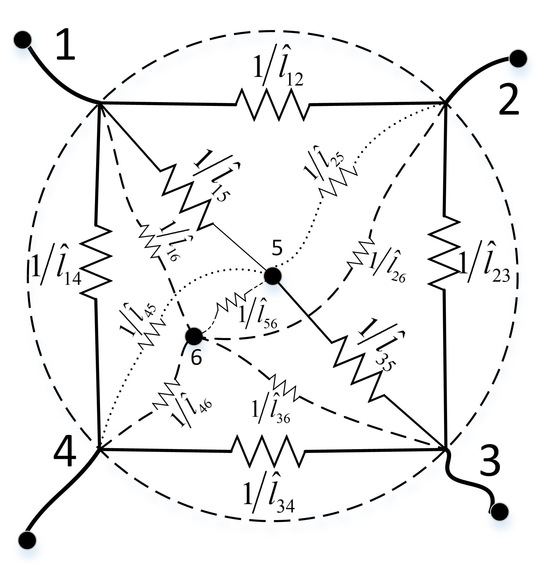
Consider a electrical network . A finite, simple, connected circular planar graph , is a graph embedded in a disc on the plane bounded by a circle as shown in Fig.1. The set is the set of nodes and the set is the set of edges. The nodes are of two categories, namely, boundary nodes which lie on circle , and the interior nodes which lie in the disc as shown in Fig.1. Thus, with as the set of boundary nodes and as the set of interior nodes, respectively. The number of boundary nodes and the number of interior nodes are assumed to be known. Label the boundary nodes from to , in clockwise circular order around as shown in Fig.1.
Let be the set of boundary nodes available for voltage and current measurements. Then, the set of all nodes that are not available is . Denote by the set of boundary nodes not available for the measurements.
The conductivity function , assigns to each edge , a positive real number , known as the conductance of . The resistance of the edge then is , . Let and . The resistance distance, , between any two nodes , is the effective resistance measured across nodes and . Let , where , be the resistance distance matrix with entries . A quantity related to the resistance distance is the so-called Kirchhoff’s index, which is the sum of the effective resistances across all pairs of nodes,
| (1) |
Since the network is passive with no internal sources, the resistance distance between any two available boundary nodes is obtained by applying a known voltage across them and measuring the current induced at the node. The resistance distance then is simply the ratio of the applied voltage to the induced current. For the nodes available in , measure the resistance distances. Denote the set of measured resistance distances by . Thus, we know a submatrix of the resistance distance matrix which is with entries taken from .
Problem 1
Let the Kirchhoff’s index , , , and , be known. Further, let is available from measurements. Then,
-
1.
Estimate the resistance distance matrix corresponding to unknown .
-
2.
Construct the topology using the estimated and compute the edge weights , of .
To solve the problem 1, we first exploit the relationship between the resistance distance matrix and the Laplacian matrix to recover the topology. Furthermore, several properties of the resistance distance are also used to formulate an intermediate optimization problem that allows us to construct from .
A detailed multistage topology reconstruction process is explained from section 3 onwards. Before this, we briefly explain the relation between the resistance distance and the Laplacian matrix, and the properties of the resistance distances.
2.1 Laplacian and Resistance Distance Matrix
The Laplacian matrix corresponding to any graph is a symmetric matrix , defined as follows:
| (2) |
It is shown in [15], [26] that the resistance distance is related to the Laplacian matrix as follows:
| (3) |
where, , , and is vector of ones. Using equation (3), we express as,
| (4) |
Further, let and Then
| (5) |
For more detailed exposition on resistance distance, refer to [15], [26].
2.2 Triangle Inequality & Kalmanson’s Inequality
The triangle and Kalmansons inequality forms two important constraints to determine unknown entries of the resistance distance matrix in our work.
The resistance distances in a satisfies the triangle inequality[27], which is elucidated in Theorem 2.
Theorem 2
[27] For any three distinct boundary nodes in CPPR such that , the resistance distances , and satisfies,
For enforcing the triangle inequality constraints, we choose node indices such that atleast one node is from and other nodes from , then define a set then, all elements of this set must be non-negative and we denote this constraint by . Next, we discuss another important property of resistance distances for a CPPR electrical network, viz. the Kalmansons property.
Theorem 3
[10] For any four boundary nodes of CPPR , satisfying , the resistance distances satisfy,
| (6) |
For enforcing the Kalmansons inequalities as constraints, we first select from valid boundary node indices say atleast one boundary node index from and remaining boundary node indices from . Then, impose following Kalmansons inequalities,
| (7) |
We collect all such Kalmansons inequality constraints in the set .
Since, all elements of the set are non-negative, we therefore denote by a list of all feasible Kalmansons inequality conditions on resistance distances defined on .
In the next section we present the network initialization method which is the first stage of the multi stage topology reconstruction approach.
3 Network Initialization
3.1 Construction of
Since no information on the structure of is known apriori, we first construct a maximal planar resistor switch network over the boundary nodes, abbreviated as . In short, a is an electrical network formed by embedding a network of resistors and switches on each edge of a maximal circular planar graph.
On boundary nodes, we construct a special planar graph known as a maximal circular planar graph. Graph is maximal in the sense that addition of one more edge makes it a non planar graph. Let be a planar graph on boundary nodes, then,
Definition 4
(Maximal circular planar graph) is said to be a maximal circular planar graph on boundary nodes if,
-
•
it has boundary nodes arranged in a circular clockwise direction on circle ,
-
•
On boundary nodes we construct a graph with edges, which is a maximal planar graph [28].
The construction of is done in three step, which are as follows,
-
1.
in the first step, we construct a maximal circular planar graph .
-
2.
In the second step, we construct a network, which is an interconnection of resistors and switches. Let us call this a resistor switch network (RSN). Number of resistors and switches are decided based on value . An appropriate combination of and switches in a RSN induces a resistance value.
-
3.
Finally, replace each edge in by a RSN to construct a .
We now briefly explain each step in the construction of . In the first step, we construct a circular graph with edges on boundary nodes, to ensure maximal planarity as mentioned in Definition 4. In the second step, we construct a RSN based on value , as shown in Fig.2.
Let us call this general RSN across boundary nodes and as ; also, let . Each has two components, i.e., component A and component B as shown in Fig.2, which helps approximately generates all admissible values of edge resistance , for appropriate combinations of switches. This is explained briefly below.
3.1.1 Component A
Component A of is composed of a boundary node , nodes and the corresponding switch variables , . Since, each switch variable can take either or , there are switch combinations which induces resistances values . The minimum resistance value induced by component A, i.e. , is generated when all the switches are on, whereas the maximum value is . Switch positions in component A generates only resistance values in and hence has limited resolution and capability to generate other numbers in the mentioned range. Therefore, to improve this, we add one more component, named component B, as shown in Figure 2.
3.1.2 Component B
Component B of is capable of generating fractional edge resistances values , . It is composed of resistances, constructed in such a way that each edge resistance is equal to the parallel combination of resistances as shown in Figure 2. Component B is connected to component A by a switch .
The designed approximately generates any resistance value in the range ; other designs can also be explored to generate better resistances values in the range .
Finally, to construct a we replace each edge in by a . This concludes the construction of . An example on construction of in given in Example 6 for better understanding.
Remark 5
The number of edges in an unknown network is less than or equal to , as discussed in Definition 4. To identify such edges, a switching-based network structure is adopted here. The switch helps decide whether an edge is present in an unknown topology, based on the available resistance distance measurements and the Kirchhoffs index.
Example 6
Let and are known apriori. The first step is the construction of , on boundary nodes, as shown in Fig.3.
The second step is constructing the resistor switch network across the boundary nodes , based on , as shown in Fig.4.
Component A of has three switches , therefore, there are switch combinations that induce resistance values. These resistance values are . The minimum value is obtained when all switches in component A are , and the maximum value is other than . Component B is added to component through a switch , where and . The designed , approximately generates resistance values in the range ( not included).
In the last step, we replace each edge in by a resistor switch network. The resultant is as shown in Fig.5.
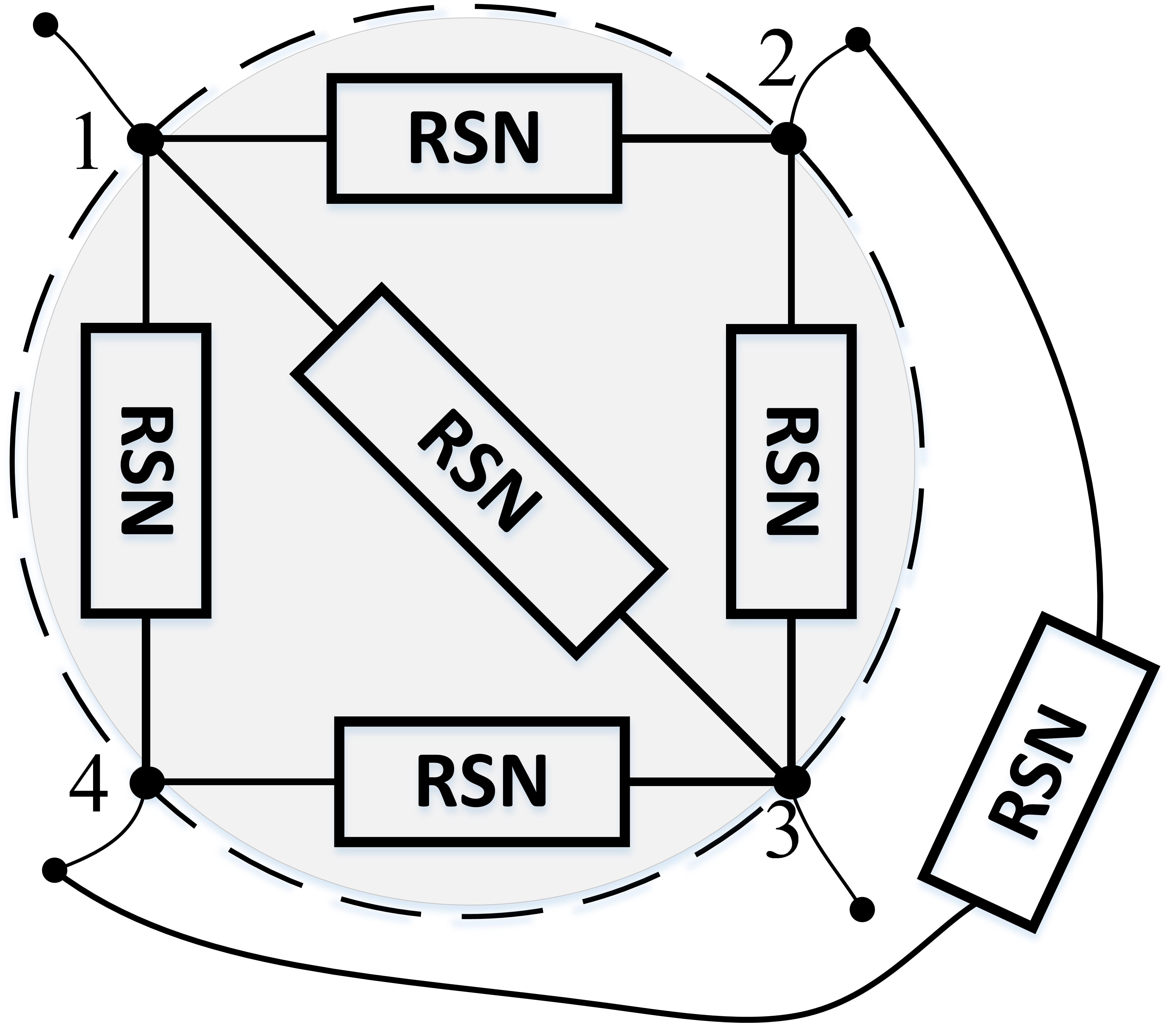
Let the constructed be called as . Where , is the set of all nodes and is a set of all edge in . Let is a set of all node pairs connected through a resistor and switch, for example, in Fig.4, a node pair and are connected by a resistor and a switch, therefore . The conductance function . The Laplacian matrix of is , defined as follows.
| (8) |
The size of is large compared to the Laplacian matrix of unknown network . Now, in , we aim to determine a combination of switch positions such that is minimum, where and is the resistance distance across boundary nodes in . The resistance distance are function of switch positions. In the next section, we will formulate an optimization problem that helps decide the switch positions in .
3.2 Determining Switch Positions in
The switch position variables in each are unknown. Therefore, let be a vector of switch variables, where . To determine we formulate two optimization problems, labelled as problem and . is primarily used to compute the estimates of the unknown resistance distances . Let the estimates be represented as . The problem uses the known resistance distances and the estimated resistance distances to determine the status of switch variables. The problem is formulated below first and then is explained.
3.2.1 Optimization problem
Consider equation (5), from which we have,
| (9) |
where . There are such linear equations. From the definition of X we have , which is framed as linear equations, here . Since, Kirchhoffs index is known, equation (1) is also posed as a linear equation.
Now, club linear equations as a system of linear equations, as shown in equation (10),
| (10) |
Where is a vector of unknowns, whose elements are obtained from unknown matrix , is the vector known resistance distances, appended by value .
Now, consider equation (10) and let be a transformation such that . To compute the estimates of unknown resistance distances , solve
The solution to the problem is , from construct , i.e, . Then, compute estimated resistance distance matrix from using relation (5). Therefore, the estimated resistance distances are .
3.2.2 Optimization problem
The optimization problem is formulated such that the resistance distance error are minimum. Here, is the measured resistance distances and is the estimated resistance distance, is the resistance distance of across boundary nodes . Now, let the be vector of measured and estimated resistance distances, and be a vector of resistance distances corresponding to , which is a function of switch positions . Then, is the resistance distance error vector, which is to be minimized with respect to switch positions . The is defined below,
| s.t | |||
In , weighting matrix is a diagonal matrix with positive entries. The entries of W, say weighing are fixed to , whereas the entry weighing are constrained between to , as posed in . The terms in are difference of convex functions, therefore, the formulated optimization problem is a difference of convex programming problem [29]. is solved using disciplined convex concave programming package[29], [30].
For computing initial guess various methods have been mentioned in [29]. We present a novel alternate method to construct an initial guess for , explained in appendix C. This alternate method works well in our experience in this work.
A term in objective function is convex if and only if each is convex with respect to the edge conductances. The convexity of resistance distance with respect to the edge conductance is discussed in [15]. Here, we mention the same as proposition 7, and an alternate proof is presented in A.
Proposition 7
Let be a vector of edge conductances of any . The resistance distance is a convex function of .
The solution to is . However, we need elements of to be either or . Therefore, to arrive at a boolean vector, we apply the Round-Down algorithm[31].
3.2.3 Round Down Algorithm
Constraining to be either or leads to non convex constraint, therefore is constrained to be in between . The solution vector is converted to a boolean vector using the Round-Down algorithm[31]. The Round-Down algorithm is based on Proposition 8, as given below,
Proposition 8
[31] Consider a boolean function and let . There exist boolean vectors , for which .
Therefore, there exist a boolean vector , which minimizes the objective function in . To facilitate the computation of boolean vector , the derivative of , is defined as,
| (11) |
The Round-Down algorithm checks whether each element in vector , say . If yes, then, check the derivative . Based on the sign of , the element is flipped to 0 or 1, and then the triangle and Kalmansons constraints is checked. The Round-Down algorithm is given in detail in Algorithm 1.
The boolean vector contains the appropriate switch positions which are used to construct an equivalent initial resistive network. Let us call this initial network as an auxiliary network , where . The initial network gives us an initial topology which will be used in next stage of reconstruction. The edge conductances will be used in the next stages as an initial guess in an optimization problem .
Since the interior nodes are not taken into account in , a structured way of embedding interior nodes is needed. Placement of interior nodes in is explained in detail in section 4.
4 Heuristic of Placement of Interior Nodes
Consider a modified network constructed from initial network by replacing each edge conductance with an unknown . Here, and . Let be the vector of unknown edge conductances in , also let be a corresponding edge resistance vector. In this section, we aim to search for edges in to introduce interior nodes. To identify such edges, we formulate an optimization problem and solve for . The problem is reformulation of with addition of a Kirchhoff’s index error term in the objective function and a relaxed edge conductance constraints, as given below,
| s.t | |||
In , is the Kirchhoff’s index corresponding to network and is a function of unknown edge conductances. The initial guess for is equal to the edge conductances obtained in initial network.
The edges where interior nodes are to be placed is based on the edge resistance vector , which is the solution to problem . To understand this, consider for an instance that we introduce an interior node, say , on a resistive edge . This results in two new resistive edges, and . Each of these resistive edge can take a maximum edge resistance of as per the assumption. In some cases an edge with interior node, say , is likely to have an edge resistance greater than . To detect such edges, we examine solution and collect all the edge resistances greater than . Arrange them in descending order and store it in another vector, say . Let be number of elements in . If,
-
1.
, place interior nodes on edges. The edges corresponds to first edge resistances in . Whereas, interior nodes are placed as dangling nodes.
-
2.
, place interior nodes on edges. The edges corresponds to first edge resistances in .
Once the placement of interior nodes are known. The next natural question is how are the interior nodes connected to the remaining nodes?. Next section answers this questions in detail.
5 Constructing Planar Networks and Rewiring
5.1 Planarity checking and planar construction
Once we proximately know the positions of interior nodes, we place interior nodes in appropriately. Then, connect the interior nodes to every other node, keeping the edges in intact. Let the resultant graph be called as , where and . Connecting interior nodes to every other node may render the resultant network non-planar. Since the aim is to reconstruct a planar resistive network, we, therefore, extract a set of planar networks from . Next, we answer two related questions, 1. how to decide whether the graph is planar or non-planar? 2. If the graph is non-planar, how to extract planar graphs?
5.1.1 Planarity Testing & Construction
Let us define a transformation which maps a graph onto a plane such that, 1. every vertex in is mapped to a distinct point in plane, 2. all edges in are mapped to a simple curve on a plane. Vertices accompanying the edges are mapped as mentioned in point 1. The diagram on the plane is called an embedding of . A graph is said to be planar iff no distinct curves cross each other in . is then said to be a planar embedding of on a plane. Before presenting an algorithm for planarity testing, we define some essential terms to understand the algorithm. First, we need a systematic way to explore an undirected graph ; to do this, we use depth first search (DFS). For detailed explanation on DFS refer to [32]. The DFS algorithm partitions the edge into two classes, i.e. 1. tree arcs, and 2. back edges. These are defined as follows,
Definition 9 (Tree arc & Back edges)
A directed edge say , is a tree arc, represented as , if . Similarly, a directed edge is a back edge, represented as , if .
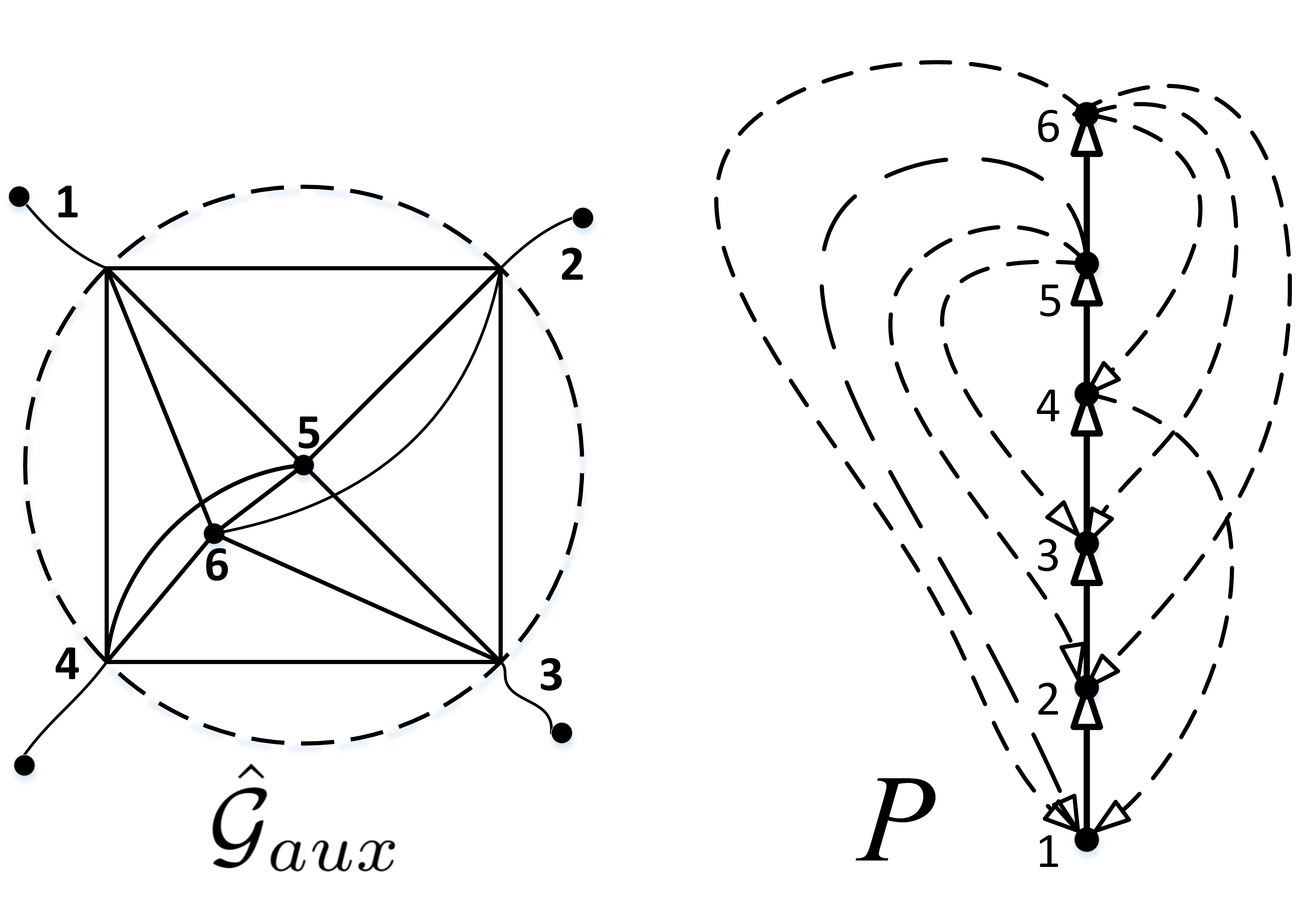
If such partitions exist for , we then construct a palm tree diagram for . For example, the palm tree representation of is shown in Fig.7. This corresponds to an example , as shown in Fig.6(d).
To test a graph’s planarity, we apply DFS to and construct a palm tree representation . Then apply a modified Auslander, Parter, and Goldstein’s algorithm[33], [34]. This algorithm
- •
-
•
Algorithm then embeds cycle first, and then sequentially embeds each segment, while also checking whether the embeddings cross each other. If there is a crossing then is non planar.
-
•
When is non planar, the algorithm detects the embedded segments which crosses the recently added segment’s embedding. Then constructs two planar embeddings, such that one of them has only recently added segment and deleting the embeddings crossing it. Whereas, in other planar embedding, the recently added segment is deleted and all other embeddings are preserved.
The detailed description of modified Auslander, Parter, and Goldstein’s algorithm is given in D.
All the planar embeddings constructed out of non planar graph is transformed back to planar graphs, after applying Algorithm 7 in D. Let the set of all planar graphs be .
6 Rewiring
For every graph , where , construct a resistor network , where . The conductivity function is unknown. Therefore, let be a vector of unknown conductances of network . Our aim now is to determine possible rewirings and assignment of the edge conductances in . This is done by formulating a sparse difference of convex optimization problem , as given below,
| s.t | |||
is the solution of the convex optimization problem . If some of the elements of solution vector then apply the round algorithm. The round algorithm based on the sign of derivative (similar to defined in equation (11)) assigns elements in to either or . Then, again run with this modified as the initial condition.
Solve for each and let be the set of solution vector. Choose from a conductance vector which has a minimum value of . Such gives us a reconstructed network corresponding to unknown network .
We derive the gradient and hessian of resistance distance error and the Kirchhoff’s index error, in B, which will be useful in solving , and .
7 Example
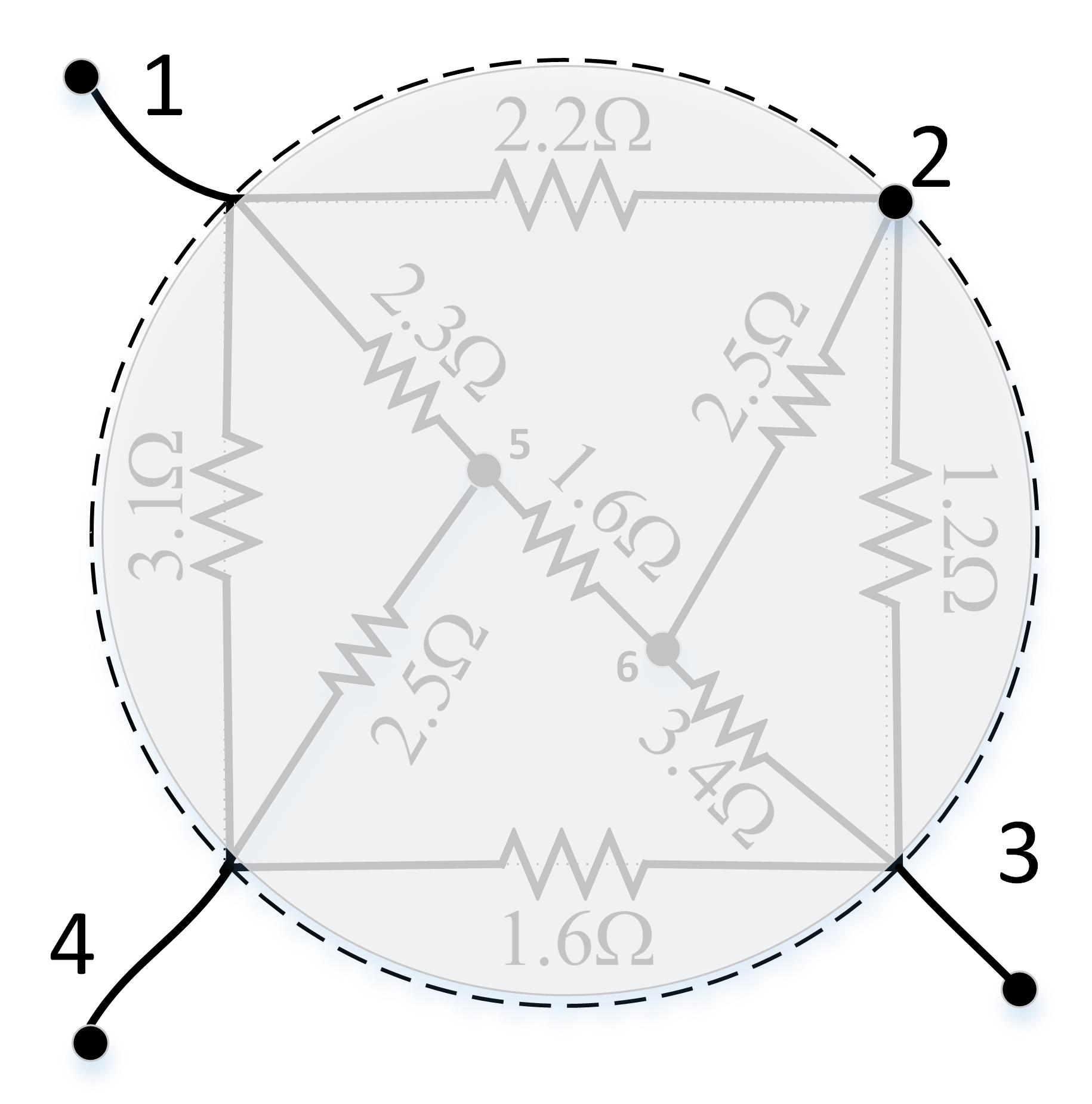
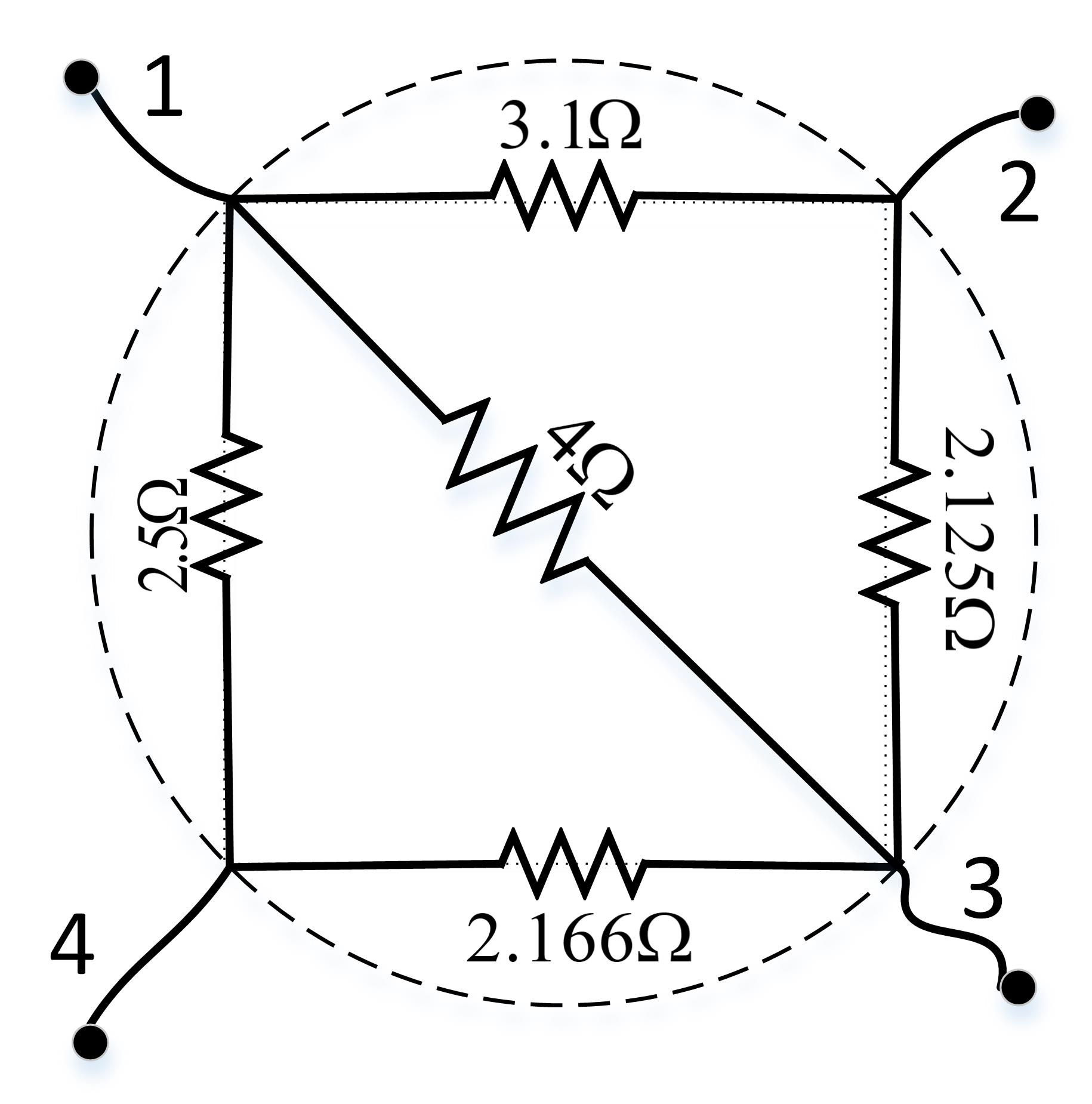
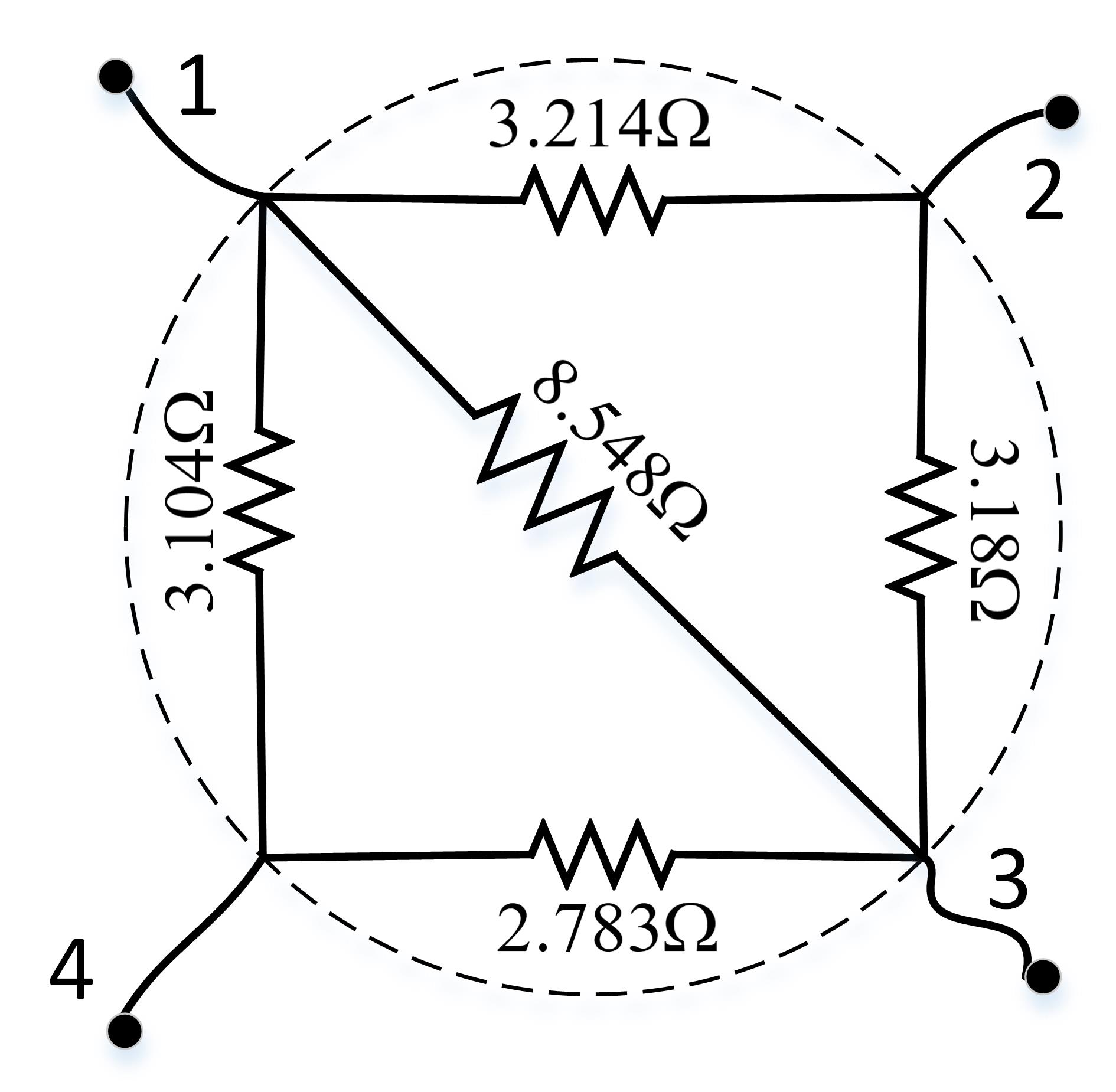
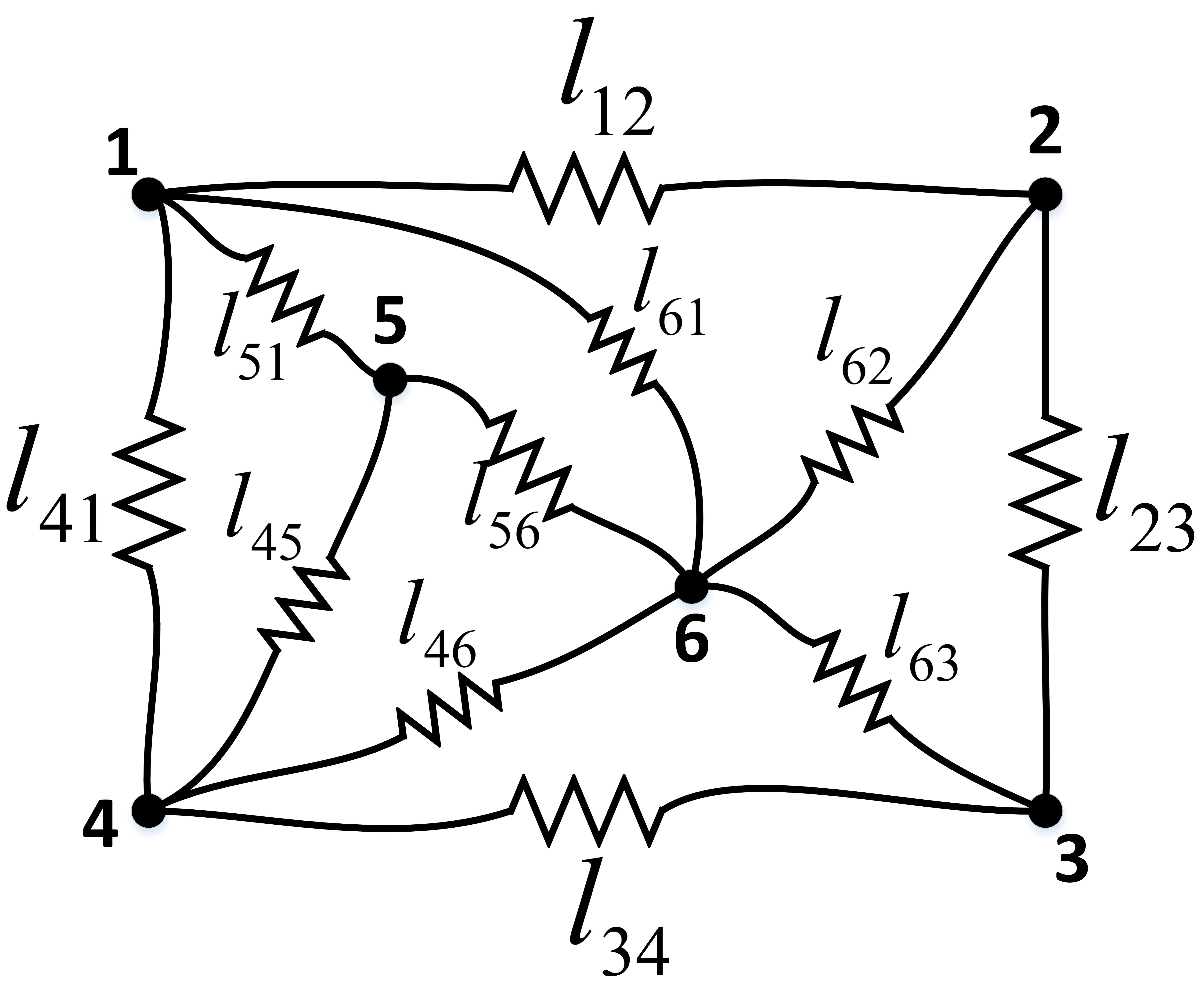
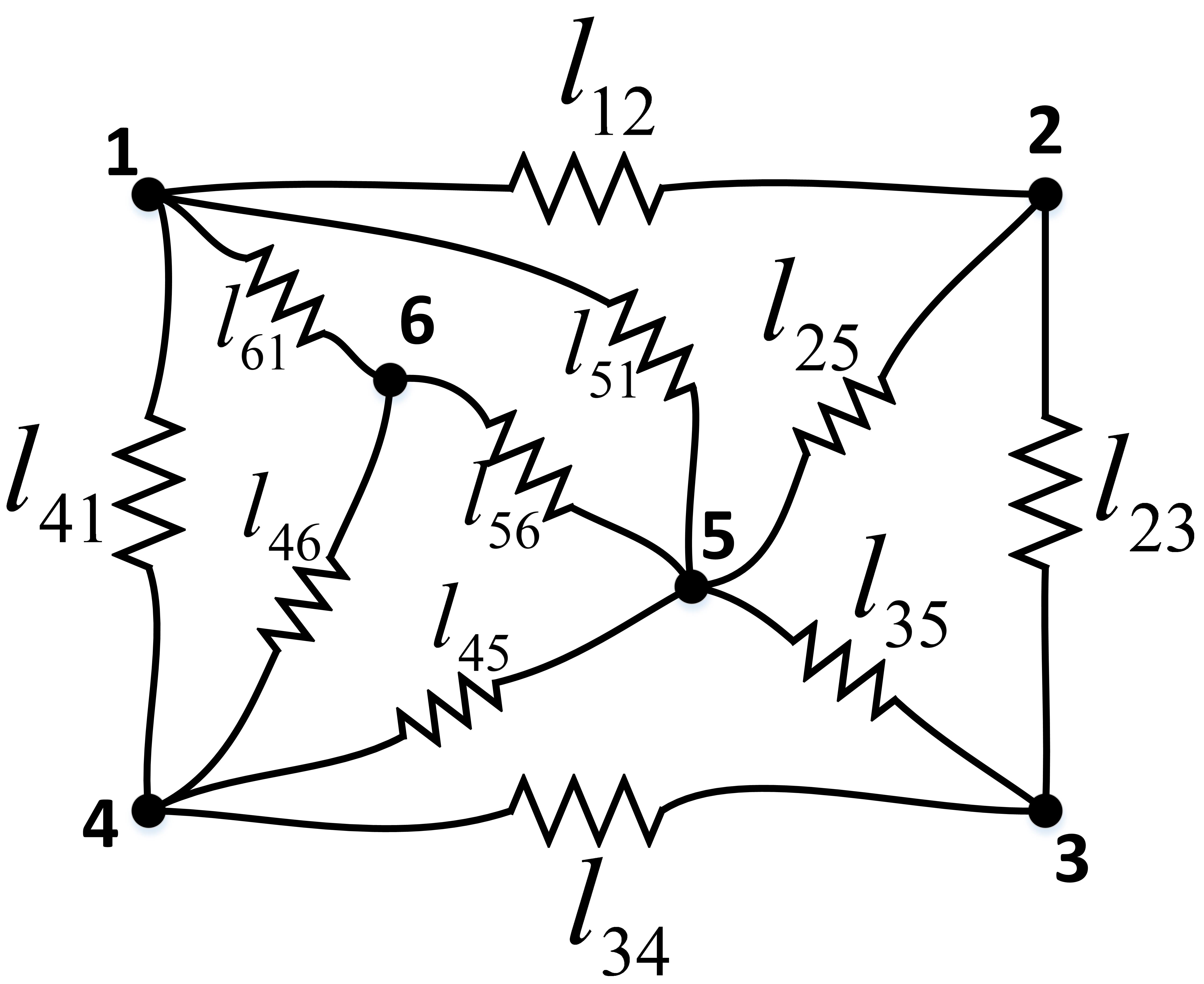
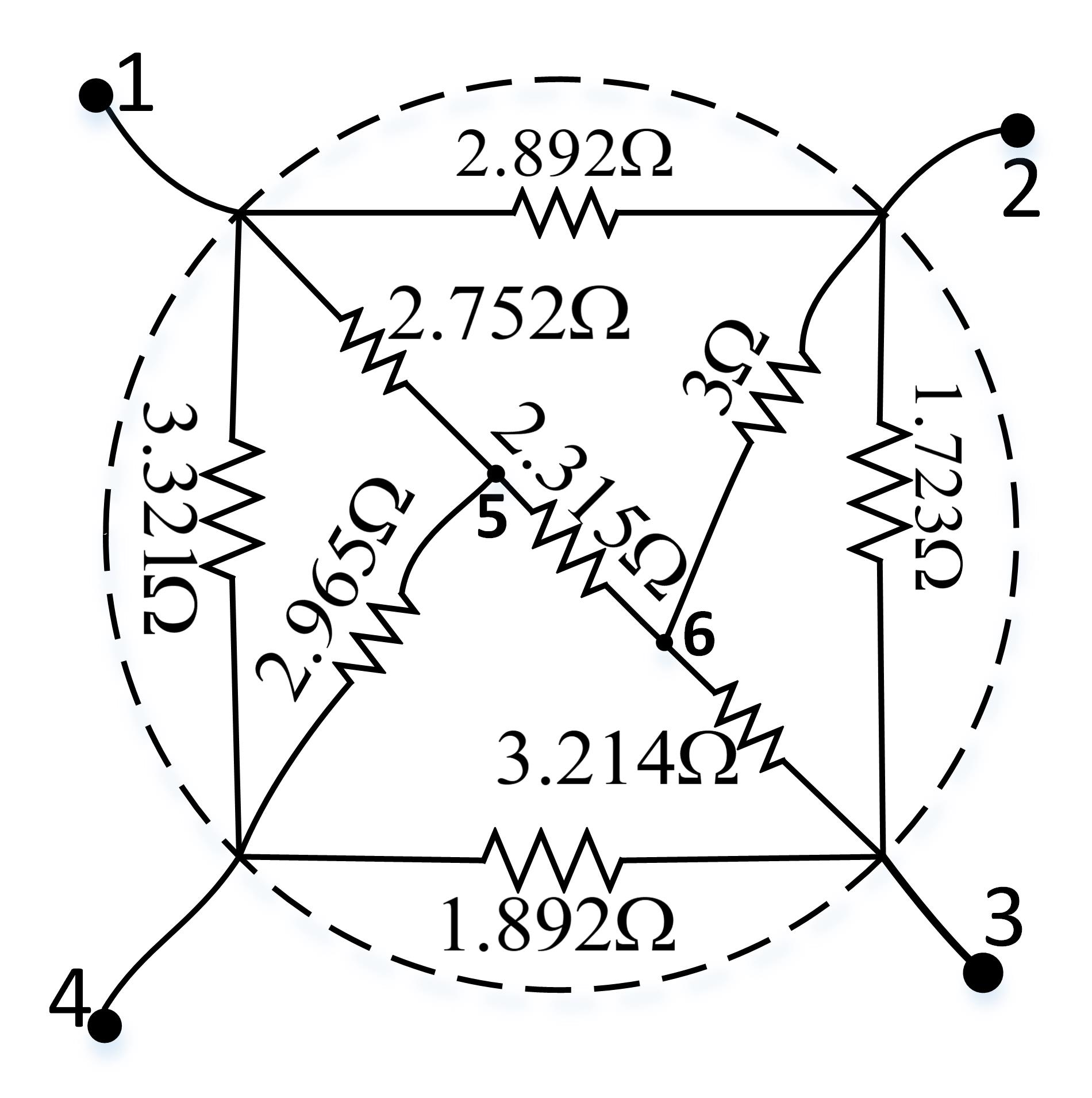
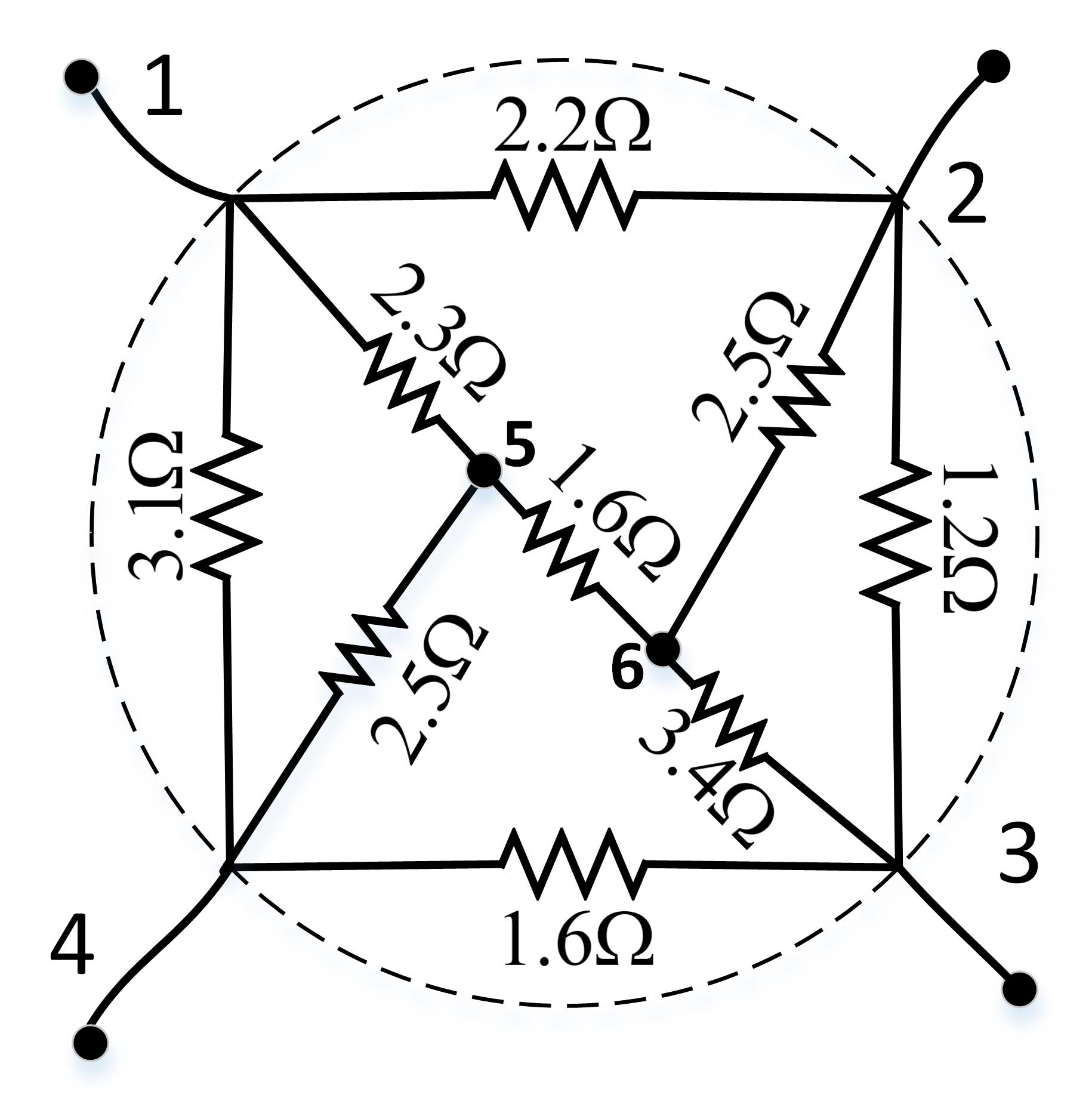
Let us consider an unknown network as shown in Fig.6(a). The following are the knowns , , , , , , and we have . We construct an appropriate as shown in Fig.5 in Example 6. Formulate an optimization problem to compute the estimates and, then solve to find an optimal switch combination. The solution to this problem is , shown in Fig.6(b). Now, to place interior nodes appropriately, apply heuristic method. Solution to is shown in Fig.6(c). Then, by examining the solution edge resistance vector , interior node is placed on edge and interior node is a dangling node as shown in Fig.6(d). Now, connect all the interior nodes to every other node to get a network as shown in Fig.6(d). The network may be non planar, we therefore apply modified Auslander, Parter, Goldstein algorithm and construct corresponding planar resistive electrical networks and as shown in Fig. 8(a) & 8(b). It can be seen that the networks are structurally similar with different numbering for interior nodes. Therefore, solve problem for or to get the solution or . The reconstructed network corresponding to an unknown electrical network is shown in Fig. 8(c), and the original network is shown in Fig 8(d). The authors would like to acknowledge the availability of the source code related to this example on GitHub.
8 Discussions
8.1 Number of Measurements
In equation (10), if all nodes, i.e. , are available, we get a unique solution to the reconstruction problem. If all the boundary nodes are available for performing experiments, the interior nodes are still not available. In such case we will always have infinite number of solutions satisfying equation (10). Hence, we can construct infinite number of electrical networks satisfying available resistance distance measurements. Therefore, to search for a valid network, we introduce the triangle and Kalmansons inequality constraints.
8.2 Methodology
The methodology proposed works well for small networks. As the number of boundary nodes increases, the number of edges in the maximal planar graph increases almost exponentially. The lower bound on the number of edges for a given number of vertices is given in [35].
In the construction of , as the value increases, number of switch positions to be optimized also increases, thereby increasing the complexity of problem . The , in general, constructs a global overestimator of the objective function and solves the resulting convex subproblem with cheap per iteration complexity[29].
The proposed method depends on the planarity testing algorithm and extracting admissible planar embeddings simultaneously. This process becomes computationally heavy for large networks. The number of planar embeddings depends on the number of dangling and non-dangling nodes. Also, as the number of dangling nodes increases, the number of admissible planar embeddings increases. The Auslander, Parter and Goldsteins algorithm has complexity of , where is the number of nodes in graph.
8.3 Error
Three major sources of errors that induces error in the reconstructed network are,
1. number of available resistance distance measurements,
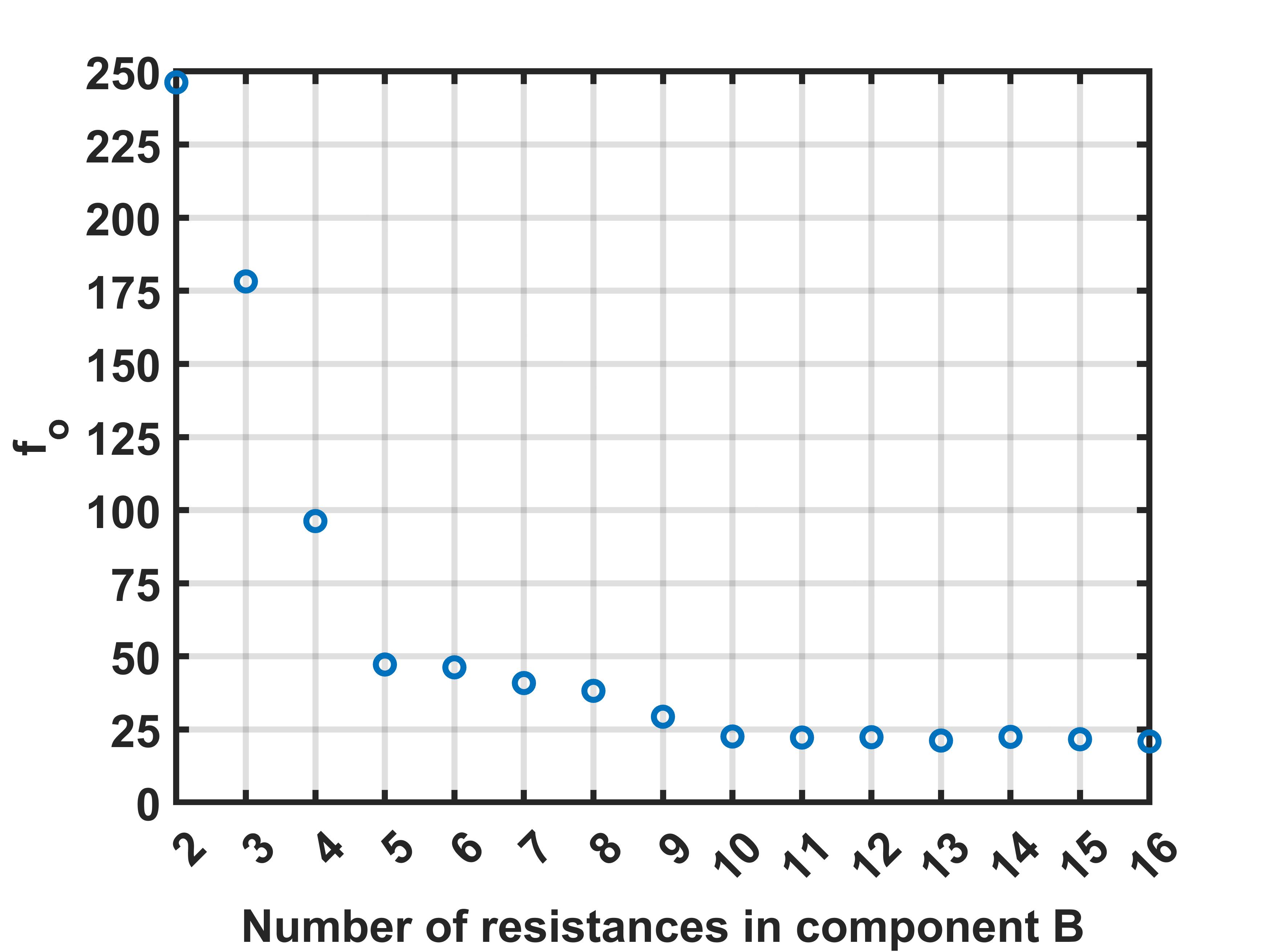
2. number of resistances in component B of the RSN, in ,
3. choice of initial conditions for optimization formulation.
As the number of available resistance distance measurements increases, switch positions can be tuned appropriately to get a better . Therefore, more resistance distance measurements will lead to a reliable , and this will further lead to proper reconstruction of the network.
Let us consider a case wherein the available boundary measurements can properly reconstruct a network. We now consider the effect of the number of resistances in component B of RSN on the value of corresponding to . It is seen that, as the number of resistances in component B increases, the value of decreases for some values and then remains almost constant, as shown in Fig.9.
Initial guess values fed into the optimization routine must be chosen judiciously, for proper network reconstruction. The quality of reconstructed network is sensitive to the choice of guesstimate of switch variables vector for . Therefore, a novel method for choosing a proper initial guess of switch positions in for is explained in appendix C.
8.4 Initial Conditions
The problems , & are implemented using a and is sensitive to initial guess. Therefore, a proper choice of initial guess is necessary to get the right solution. In problem , the initial is chosen by applying algorithms mentioned in C. The solution to the problem is . For problem , the initial guesstimate is based on the edge resistances of . Therefore, the element of , which is also the edge of is . For , the initial guesstimate is inferred from the edge resistances of network and . The is decided as follows, the edge conductance if , if and if .
9 Conclusion
We presented a multistage topology reconstruction algorithm for a general electrical network. We assume that only some of the resistance distance measurements are available, the number of boundary and interior nodes, minimum and maximum value of edge conductance and the Kirchhoffs index are known corresponding to an unknown network . We start the reconstruction process by constructing an initial network . The construction of comprises two steps; the first is constructing a maximal planar network whose edges are composed of resistors and switches in a specific configuration based on the maximum resistance value. Therefore, the switch positions decide the edge resistance. In the second step, the switch positions are decided based on the available and estimated resistance distance measurements. This is done by formulating a difference of convex programming problem involving a quadratic cost function, constrained by triangle and the Kalmansons inequalities. The resultant switch positions thus give us an initial network . The gives us an initial topology which is used subsequently for adding interior nodes.
Interior nodes are not considered in the . Therefore, we develop a heuristic approach that re-optimizes the edge resistances of initial topology of . Re-optimization involves solving optimization problem , which is a reformulation of with Kirchhoffs index and relaxed edge conductance constraints. We then examine optimized edge resistances and introduce an appropriate number of interior nodes on edges with edge resistance greater than the maximum resistance; the remaining interior nodes are considered dangling nodes.
Since the interconnection among interior nodes and between interior nodes and boundary nodes is unknown, we connect the interior nodes to all other nodes to account for all possible edges in an unknown network. This may result in a non-planar network. Therefore, we propose a modified Auslander, Parter, and Goldstein’s algorithm to get planar networks from a non-planar network. Then, each planar network’s edge conductance is computed by solving an optimization formulation similar to . A network which best satisfies the available measurements is chosen as a reconstructed network.
The proposed methodology is suitable for networks with fewer boundary and interior nodes. The computation of the initial network , the heuristic method proposed for the placement of interior nodes, and the algorithm for construction of a set of planar networks can be further improved, to improve the efficiency of the overall proposed algorithm. The Kirchhoff’s index is assumed to be known in this work, but in general, it is not known. A work in [36] computes upper and lower bounds on the the Kirchhoffs index for a weighted graph, these bounds can be used in our work by blending in these bounds into the optimization formulation. The proposed multistage topology reconstruction procedure can be generalized to reconstruct RLC networks, which are the subject of future research.
References
- [1] M. Akbaba, O. Dakkak, B.-S. Kim, A. Cora, S. A. Nor, Electric circuit-based modeling and analysis of the translational, rotational mechanical and electromechanical systems dynamics, IEEE Access 10 (2022) 67338–67349.
- [2] F. Gomez, J. Bernal, J. Rosales, T. Cordova, Modeling and simulation of equivalent circuits in description of biological systems-a fractional calculus approach, Journal of Electrical Bioimpedance 3 (1) (2012) 2–11.
- [3] F. Veldman-de Roo, A. Tejada, H. van Waarde, H. L. Trentelman, Towards observer-based fault detection and isolation for branched water distribution networks without cycles, in: 2015 European Control Conference (ECC), IEEE, 2015, pp. 3280–3285.
- [4] J. Jirkuu, J. Vilhelm, Resistor network as modeling tool for fracture detection in crystalline rocks., Acta Geodynamica et Geomaterialia 16 (4) (2019).
- [5] F. Lundstrom, K. Frogner, M. Andersson, A resistor network model for analysis of current and temperature distribution in carbon fibre reinforced polymers during induction heating, Journal of Composite Materials 56 (20) (2022) 3159–3183.
- [6] Y. Zhao, C. K. Khaw, Y. Wang, Measuring a soft resistive strain sensor array by solving the resistor network inverse problem, in: 2023 IEEE International Conference on Soft Robotics (RoboSoft), IEEE, 2023, pp. 1–7.
- [7] V. V. Cheianov, V. I. Fal’ko, B. L. Altshuler, I. L. Aleiner, Random resistor network model of minimal conductivity in graphene, Physical review letters 99 (17) (2007) 176801.
- [8] R. Rocco, J. del Valle, H. Navarro, P. Salev, I. K. Schuller, M. Rozenberg, Exponential escape rate of filamentary incubation in mott spiking neurons, Physical Review Applied 17 (2) (2022) 024028.
- [9] J. Zhu, A. Jabini, K. Golden, H. Eicken, M. Morris, A network model for fluid transport through sea ice, Annals of Glaciology 44 (2006) 129–133.
- [10] S. Forcey, D. Scalzo, Phylogenetic networks as circuits with resistance distance, Frontiers in Genetics 11 (2020) 586664.
- [11] F. Dorfler, F. Bullo, Kron reduction of graphs with applications to electrical networks, IEEE Transactions on Circuits and Systems I: Regular Papers 60 (1) (2012) 150–163.
- [12] E. Curtis, E. Mooers, J. Morrow, Finding the conductors in circular networks from boundary measurements, ESAIM: Mathematical Modelling and Numerical Analysis 28 (7) (1994) 781–814.
- [13] E. B. Curtis, J. A. Morrow, Determining the resistors in a network, SIAM Journal on Applied Mathematics 50 (3) (1990) 918–930.
- [14] E. B. Curtis, J. A. Morrow, Inverse problems for electrical networks, Vol. 13, World Scientific, 2000.
- [15] A. Ghosh, S. Boyd, A. Saberi, Minimizing effective resistance of a graph, SIAM review 50 (1) (2008) 37–66.
- [16] K. Moffat, M. Bariya, A. Von Meier, Unsupervised impedance and topology estimation of distribution networks—limitations and tools, IEEE Transactions on Smart Grid 11 (1) (2019) 846–856.
- [17] K. Soumalas, G. Messinis, N. Hatziargyriou, A data driven approach to distribution network topology identification, in: 2017 IEEE Manchester PowerTech, IEEE, 2017, pp. 1–6.
- [18] H. J. van Waarde, P. Tesi, M. K. Camlibel, Topology identification of heterogeneous networks: Identifiability and reconstruction, Automatica 123 (2021) 109331.
- [19] M. Nabi-Abdolyousefi, M. Mesbahi, Network identification via node knockout, IEEE Transactions on Automatic Control 57 (12) (2012) 3214–3219.
- [20] B. M. Sanandaji, T. L. Vincent, M. B. Wakin, Exact topology identification of large-scale interconnected dynamical systems from compressive observations, in: Proceedings of the 2011 American Control Conference, IEEE, 2011, pp. 649–656.
- [21] D. Materassi, M. V. Salapaka, On the problem of reconstructing an unknown topology via locality properties of the wiener filter, IEEE transactions on automatic control 57 (7) (2012) 1765–1777.
- [22] S. Biradar, D. U. Patil, Topology reconstruction of a circular planar resistor network, in: 2023 European Control Conference (ECC), IEEE, 2023, pp. 1–6.
- [23] D. Cox, J. Little, D. O’Shea, M. Sweedler, Ideals, varieties, and algorithms, American Mathematical Monthly 101 (6) (1994) 582–586.
- [24] S. Biradar, D. U. Patil, Topology reconstruction of a resistive network with limited boundary measurements, in: 2022 Eighth Indian Control Conference (ICC), IEEE, 2022, pp. 379–384.
- [25] J. Hopcroft, R. Tarjan, Efficient planarity testing, Journal of the ACM (JACM) 21 (4) (1974) 549–568.
- [26] P. Christiano, J. A. Kelner, A. Madry, D. A. Spielman, S.-H. Teng, Electrical flows, laplacian systems, and faster approximation of maximum flow in undirected graphs, in: Proceedings of the forty-third annual ACM symposium on Theory of computing, 2011, pp. 273–282.
- [27] M. C. Choi, On resistance distance of markov chain and its sum rules, Linear Algebra and its Applications 571 (2019) 14–25.
- [28] T. Nishizeki, M. S. Rahman, Planar graph drawing, Vol. 12, World Scientific, 2004.
- [29] X. Shen, S. Diamond, Y. Gu, S. Boyd, Disciplined convex-concave programming, in: 2016 IEEE 55th conference on decision and control (CDC), IEEE, 2016, pp. 1009–1014.
- [30] T. Lipp, S. Boyd, Variations and extension of the convex–concave procedure, Optimization and Engineering 17 (2016) 263–287.
- [31] E. Boros, P. L. Hammer, Pseudo-boolean optimization, Discrete applied mathematics 123 (1-3) (2002) 155–225.
- [32] R. Tarjan, Depth-first search and linear graph algorithms, SIAM journal on computing 1 (2) (1972) 146–160.
- [33] L. Auslander, Psv on imbedding graphs in the plane, Journal of Mathematics and Mechanics 10 (3) (1961) 517–523.
- [34] A. Goldstein, An efficient and constructive algorithm for testing whether a graph can be embedded in a plane, in: Graph and Combinatorics Conference, Contract No. NONR 1858-(21), Office of Naval Research Logistics Proj., Dept. of Mathematics, Princeton University, May 16-18, 1963.
- [35] W. T. Tutte, A census of planar triangulations, Canadian Journal of Mathematics 14 (1962) 21–38.
- [36] M. Bianchi, A. Cornaro, J. L. Palacios, A. Torriero, Bounds for the kirchhoff index via majorization techniques, Journal of mathematical chemistry 51 (2) (2013) 569–587.
- [37] V. V. Fedorov, Theory of optimal experiments, Elsevier, 2013.
- [38] K. Behrens, Planarity testing–the efficient way?
Appendix A Convexity of Resistance Distance & Kirchhoff’s Index
The convexity of resistance distance with respect to the edge conductance is discussed in [15] by omitting proof. Here, we mention the same with detailed alternate proof.
Proposition 10
Let be a vector of edge conductances of , then the resistance distance is a convex function of .
Proof 1
Consider a electrical network . Let & be vector of edge conductance’s, such that . The resistance distance is said to be a convex function if it satisfies equation (12),
| (12) |
Let be the Laplacian matrix corresponding to conductance vector , to denote its dependence on we call it . Let to be the incidence matrix corresponding to the graph , then is the column of . We can write,
| (13) | ||||
| (14) |
Taking inverse on both side, we get,
| (15) |
Without loss of generality, let and using Theorem 11, as given below,
Theorem 11
[37] If M and P are positive definite matrix, then,
| (16) |
Corollary 12
is a convex function, Since it is the sum of resistance distances.
Appendix B Gradient and Hessian
We derive gradient and hessian of and and which will be useful in solving , & . Here. can be any network in or in or in . The derivative of weighted error resistance distance across boundary nodes and , i.e., is,
| (20) |
The derivative is given as,
| (21) |
where . Then,
| (22) |
here is the column of adjacency matrix B. The second derivative of is,
| (23) |
here .
The Kirchhoff’s index [15] is given by,
| (24) |
The derivative of the Kirchhoff’s index is,
| (25) |
Whereas the second derivative is,
| (26) |
Appendix C Construction of Initial Guess for
The initial guess fed into are the initial switch positions in . We present a novel algorithm to compute an initial guess , where . The algorithm comprises of solving first. Then, using and the estimated resistance distances , an iterative algorithm is run to compute , i.e., the initial switch positions.
The estimated resistance distances computed from and the available resistance distances in set are used in the proposed iterative algorithm to get initial guess vector .
The iterative algorithm involves,
1.) computation of edge resistances, by increasing and decreasing edge resistance by ,
2.) addition and deletion of edges,
based on and . The algorithm is designed specifically to assign only integer edge resistances upto value . The iterative algorithm gives an electrical network from which an initial switch position guess is determined to be fed into .
At iteration, we consider network , where . Instead of using edge conductance, we use edge resistance for explanation in this section. The edge resistances are set to . Let the corresponding Laplacian matrix be . Then, set of resistance distances corresponding to is , and the resistance distance error set is
. Since algorithm involves deletion and addition of edges we keep track of added and deleted edges, using , the set of deleted edges and be the set of edges added at iteration. Initially, and . Let be the degree of node at iteration. If degree of any node in an edge is we call such edge as a floating edge. The algorithm starts with identifying nodes pairs, say , across which the maximum absolute resistance distance error occurs and ( is defined in section 3). Now, the aim is to increase or decrease the edge resistance such that is minimized. Hence, if , then we either delete the edge or increase the edge resistance by , whichever is better. Whereas, if then we either add an edge with edge resistance or decrease edge resistance value by . This is exemplified for iteration, given below.
At iteration, consider a network , where and . Then, is a set of resistance distances corresponding to , and a resistance distance error set
. Also, let and be non empty set, then . Now choose an index pair, say , across which maximum absolute resistance distance error occurs from set , let us denote this process of choosing as, . Then, based on the sign of and various other criteria, several operations on graph are executed at iteration. That is, if
1.) if and , then we either delete an edges (let us call this operation ) or increase the edge resistance by (let us call this operation ). Both operations are given in details as Algorithm-2 and 3 respectively.
2.) if and then, find another node pair, say , such that and .
3.) if then, we add a new edge across nodes and . This operation is called as and is presented in details as Algorithm-5.
4.) if then we decrease the edge resistance by . Let this operation be named as and is given in detail as Algorithm-6.
Each operation is briefly explained case by case below,
Case-1: if and then,
1. the edge can be deleted, or,
2. edge resistance is increased by .
Let us call an operation in point as and, operation in point as . In case-1, first implement operation , then operation on independently. Let and be the resistance distance error across after committing operation and respectively.
An operation is said to be valid if a committed operation results in improvement of resistance distance error, i.e., if then is a valid operation to commit. Now, if both are valid, then choose an operation which results in . If only any one of the operation is valid, then implement that operation. If both are invalid then find another node pair, say , such that and . Therefore, let us define a function , which helps select an appropriate operation based on , and as explained above. This function is used in Algorithm-3 and is explained in Algorithm-4.
The operations and are given in details as Algorithm-2 and 3.
Case-2: If and , then choose another node pair , across which next maximum absolute resistance distance error occurs. Then, check the sign of to decide an operation to commit.
Case-3: Now, if , then add an edge with edge resistance . Edge addition operation for case- is called as and is given as Algorithm 5 . Let be the resultant resistance distance after committing an operation , if then is an invalid operation. In case of invalid operation , find another node pair, say , such that .
Case-4: If , then reduce the edge resistance by . Edge addition operation for case- is called as and is given as algorithm 6.
If both and are invalid operations, find another pair across which next minimum absolute resistance distance error occurs.
For every computed node pair across which maximum absolute resistance distance error occurs the sign of corresponding resistance distance error is checked and accordingly operations or is carried out. Iterations are carried out till the resistance distance errors in set , i.e. eventually the resistance distance errors in set does not change significantly. The bound can also chosen based on users experience or trial and error. Let the algorithm stops at iteration, then the corresponding network is transformed into a , wherein each edges is converted to with appropriate switch positions. Then, the switch positions or the initial guess are extracted from this .
Appendix D Modified Auslander, Parter and Goldstein’s Algorithm
Let us begin the algorithm by constructing a palm tree representation . A directed tree in is a directed graph with a root vertex such that every vertex in is reachable from the root vertex, no tree arc enters root vertex and, exactly one tree arc enters every other vertex in . The relation means there is a path from to in .
To every vertex in we associate them with two numbers i.e. low points, for example, for vertex in , and are two low points. Also, to every edge in , we associate it with an integer through a function , which is used to order the adjacency list. For detailed description on low points and function refer to [25], [38].
The cycle is a sequence of tree arcs and one back edge in . Each segment, not in , can either be a back edge or a adjoined by all back edges emanating from . Let the set of all segments be . A path in a segment, say ,
is either a single back edge or a with a back edge emanating from . To identify a cycle and paths in each segments we use the path finding algorithm. In general, a path finding algorithm identifies paths using DFS and the available adjacency list. To speed up the process the adjacency list is arranged in an increasing order of values [38].
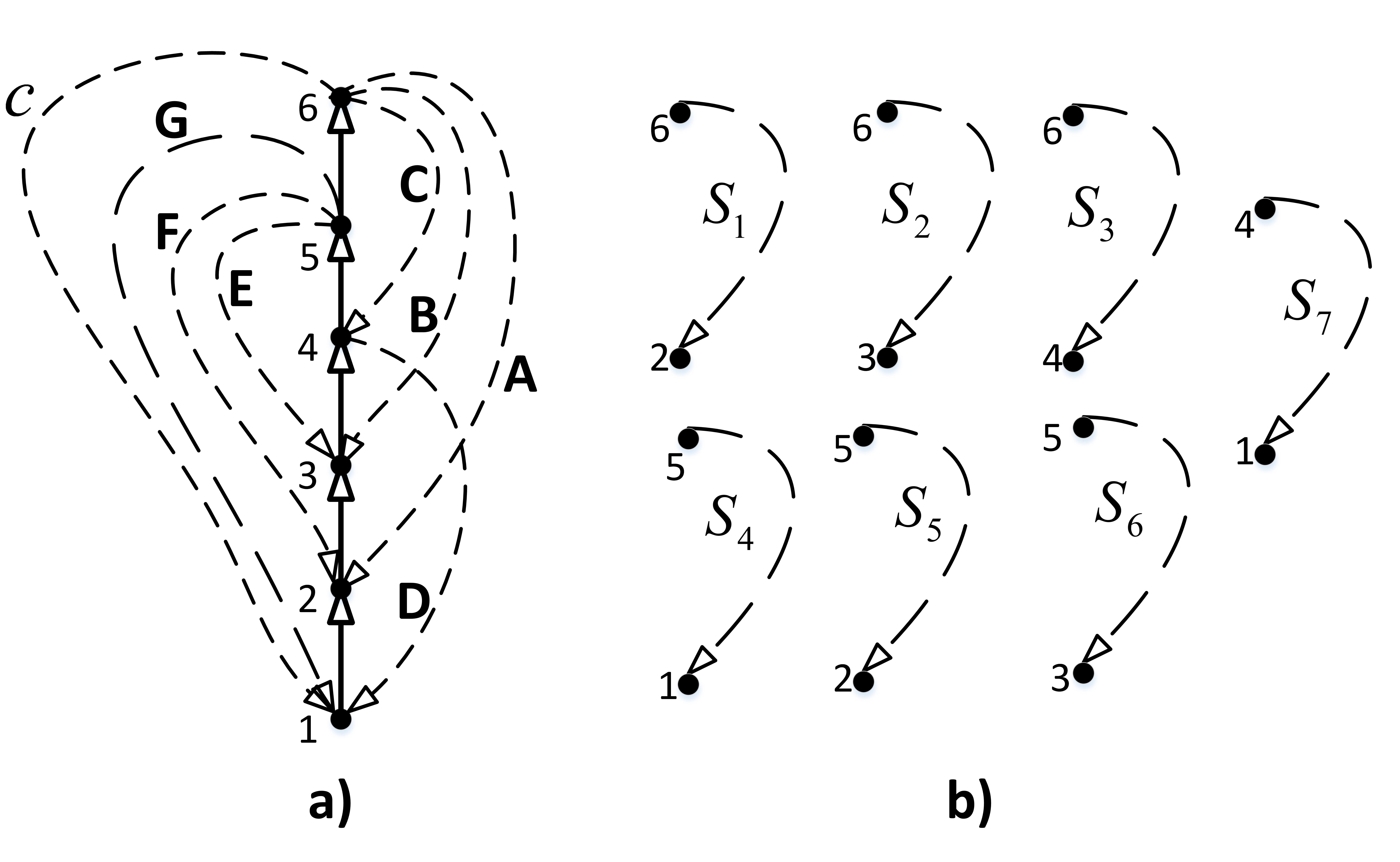
The algorithm basically finds an edge based on the ordered adjacency list, and augments it to the current path. If a back edges is encountered during exploration it is added to current path and search is considered complete. The path finding algorithm is given in detail in [25], [38]. This algorithm is illustrated for an example palm tree as shown in Fig. 10(a). The algorithm constructs a cycle which is deleted from palm tree . The deletion of from leaves behind disconnected segments, as shown in Fig.10(b) for an example. The path finding algorithm is also used for listing paths in segments. Once the structuring and path finding is over, we use this information for testing planarity. Going forward, we will briefly look into planarity testing algorithm.
The planarity testing algorithm in general does the following,
-
•
embed the cycle on a plane to get ,
-
•
embed each segment i.e. one by one on . In embedding , which is other than a back edge, we apply path finding algorithm on and generate all paths. Then, embed each path one after another on .
-
•
Every must go either on the left or right side of . When a segment is added to , certain segments, if needed, are moved from left to right or vice versa to avoid curve crossings. If all can be added to without any curve crossing, then is said to be planar.
For more detailed exposition on planarity testing refer to [25], for a concise explanation refer to [38].
Further, we explain a modification done on Hopcroft, Tarjan and Goldsteins algorithm to extract planar graphs from a non-planar graph. Let us assume that we have embedded along with some segments on plane and let be the segment to be embedded next. Consider a path in which is to be embedded on . The following lemma gives a necessary and sufficient condition for embedding ,
Lemma 1
[25] An embedding of a path from to can be added to by placing it on left (right) of iff no back edge that has already been embedded on left satisfies .
We will therefore use Lemma 1 to decide whether a graph is planar. Now, choose a side in where is to be placed. Let is placed on the left of . Check whether satisfies Lemma 1. If it does not satisfy Lemma 1, it means that there is a crossing. Therefore, to avoid crossings, move some already embedded segments on the left side to the right side of . Again, check whether satisfies Lemma 1. If it satisfies Lemma 1, embed on the left side. This strategy is shown in an example in Figure 11,
Similarly, we embed each path of one by one to completely place on one side of . We then move on to embedding the next segment.
To implement the placement of paths, Hopcroft and Tarjan[25] proposed the usage of data structure stack and to save the position of paths and segments during execution. The stack
stores all the vertices such that , and some embedded back edge enters from left. Stack is defined similarly wherein back edges enter from the right. Implementation of stack and is shown in an example in Figure 11.
Consider a case of embedding a path, say , of some segment on the left side of . Update the stacks and appropriately and check that the embedding satisfies Lemma 1. If it does not satisfy, it means that the embeddings of segments are crossing on the left side. Therefore, shift appropriate segment from left to the right of to avoid crossings on left side, and update the entries in and . Again check whether Lemma 1 is satisfied on the right side of . If it does not satisfy then we say that the graph is non planar. At this stage, we extract planar graphs from a non planar graph. The embedding cannot be placed either on the left or the right side of . Therefore,
-
•
first place on the left side of and update stack .
-
•
Find all the instances where the already embedded back edges violate lemma 1. We call such back edges as blocking segments and remaining segments as non blocking segments.
-
•
The and blocking segments cannot stay on the left side of for maintaining planarity. We therefore construct two planar embeddings, one comprising of and all non blocking segments and, other containing only blocking segments and non blocking segments.
-
•
Then, check whether all the edges of are present in the constructed planar embeddings. If not, reject that planar embedding from further analysis.
The above procedure can be understood from an example in Figure 12, wherein embedding leads to non planarity. On the left side, the blocking segments are and all remaining segments are called the non blocking segments with respect to . Both planar embeddings are shown in Fig.13.
Now, for each planar embeddings check whether all the edges of are present in it. If not, reject that planar graph from further analysis. In Fig.13(b) the edge is not present, therefore it is not considered for further analysis. Similarly place on the right side of as shown in Fig.12 (b). Find the blocking and non blocking edges with respect to the . The segments are the blocking segments. The planar embeddings corresponding to this is shown in Fig.14
A generalised algorithm is given in Algorithm 7. Every time a path is to be embedded Algorithm 7 is invoked.