Bidding in Ancillary Service Markets: An Analytical Approach Using Extreme Value Theory

Abstract

To encourage the participation of stochastic distributed energy resources in Nordic ancillary service markets, the Danish transmission system operator, Energinet, has introduced grid codes requiring a minimum 90% reliability for the full availability of reserve capacity bids. This paper addresses the bidding strategy of flexibility aggregators under Energinet’s reliability requirement by proposing a chance-constrained optimization model. An analytical solution is developed using ideas from extreme value theory, focusing on the “tail” of the empirical data used for flexibility estimation, capturing extreme events where failures are more likely to occur. The proposed model is applied to an electric vehicle aggregator participating in the Nordic market for frequency containment reserve for disturbances (FCR-D). Our results from a realistic case study show that the proposed analytical solution outperforms a commonly used sample-based approach in terms of out-of-sample constraint violation rate.

I Introduction

I-A Background and Motivation

Flexibility aggregators can pool and manage distributed energy resources, providing services such as frequency regulation and load balancing to support grid stability. This study focuses on electric vehicle (EV) aggregators that participate in frequency-supporting ancillary service markets in the Nordic region [1]. Due to the stochastic nature of EV charging behavior and availability, ensuring reliable participation in these markets presents significant challenges, requiring strategies to manage uncertainty in the aggregator’s flexibility supply.

To facilitate the participation of flexible yet stochastic resources in ancillary service markets, the Danish transmission system operator (TSO), Energinet, has introduced grid codes that establish a minimum 90% reliability requirement for the full availability of ancillary service bids [2]. By explicitly setting a failure threshold of 10%, which allows for partial or full unavailability of the ancillary service bid, this requirement encourages resources with uncertain consumption or production baselines to bid their flexibility. This, in turn, increases the supply of such services, potentially reduces service prices, and lowers the TSO’s procurement costs. However, accommodating this uncertainty in service availability during activation events may compromise grid security.

This paper takes the aggregator’s perspective to explore how to exploit this requirement. The investigation of its grid security implications, as well as the extent to which the TSO must purchase additional volumes of services to ensure grid security at a desired confidence level, is left for future work. To meet the 90% reliability requirement, aggregators must employ optimization techniques that incorporate probabilistic constraints to manage uncertainty while ensuring compliance with TSO requirements. Chance-constrained optimization is a natural choice for this task.

The paper addresses the bidding strategy of an EV aggregator using the minimum 90% reliability requirement to place hourly reserve capacity bids in the Nordic ancillary service markets. Without loss of generality, we focus on the market for frequency containment reserve for disturbances (FCR-D). Bidding decisions are made in the day-ahead stage, with uncertain future consumption from the EV aggregation. The main challenge is modeling uncertainties in EV charging patterns while adhering to the TSO requirement. We also explore how the aggregator’s strategy would change if the TSO adjusts the requirement. As our main methodological contribution, we develop a chance-constrained optimization model using concepts from extreme value theory and propose an analytical reformulation. This contrasts with the commonly used sample-based approach, which would require an increasing number of samples to model the underlying uncertainty.

I-B Literature Review

Energinet has taken a leading role among European TSOs by implementing grid codes that define the requirements for stochastic, flexible resources providing ancillary services. Research on bidding strategies for aggregators of flexible resources, constrained by these grid codes, has explored various techniques to manage the uncertainties involved in service delivery. These techniques include robust optimization [3], distributionally robust optimization [4], and optimization methods incorporating both chance constraints and conditional value-at-risk constraints [5], often reformulated using historical samples.

A common approach to solving optimization problems with uncertainty is scenario-based methods, where uncertainties are represented by a finite set of scenarios sampled from the underlying probability distribution or empirical data. While straightforward, these methods often require a large number of scenarios to accurately capture the underlying uncertainty, leading to increased computational costs [6, 7]. An alternative approach involves approximation techniques or analytical reformulations for specific types of probability distributions. These methods convert optimization problems with probabilistic constraints into analytically tractable forms, enabling more efficient solution methods [11, 8, 9, 10, 12].

A relatively underexplored but promising area in optimization under uncertainty is the analysis of the “tail” of the data, which focuses on the extreme events where failures are more likely to occur. While traditional approaches often use tail behavior or extreme values for post hoc risk assessments, there is growing interest in embedding this analysis directly into the optimization process, particularly in energy systems and resource aggregation. This gap presents an opportunity to integrate extreme value theory into chance-constrained optimization models. By doing so, decision-making under extreme uncertainties can be enhanced without the need for a large number of samples, as required by conventional scenario-based approaches. In this direction, [13] combines large deviation theory with convex analysis and bilevel optimization to derive tractable formulations that can be solved using standard solvers, assuming Gaussian mixture distributions.

To the best of our knowledge, this paper is the first to propose a framework that integrates ideas from extreme value theory into chance-constrained optimization for optimizing the bidding strategies of aggregators of stochastic flexible resources in ancillary service markets, while also incorporating and analyzing the impact of real-world market regulations.

I-C Contributions

This study develops a chance-constrained optimization model for an EV aggregator in Nordic ancillary service markets, accounting for the stochastic consumption baseline of EV fleets. By applying concepts from extreme value theory to analyze the tail behavior of EV charging patterns, the model focuses on rare, high-impact events that could lead to constraint violations and, consequently, unsuccessful flexibility service delivery. This approach improves risk characterization and ensures the model effectively handles worst-case scenarios. An analytical solution is provided that is less computationally demanding compared to commonly used sample-based methods. Additionally, the study explores how varying failure thresholds set by Energinet impact the ancillary service market participation of the EV aggregator, offering practical insights for both aggregators and the TSO on how failure thresholds influence bidding strategies and ancillary service supply.

I-D Paper Organization

The remainder of this paper is organized as follows: Section II provides the necessary preliminaries for understanding the subsequent sections. Section III presents the formulation of the chance-constrained optimization problem. Section IV outlines the methodology for the analytical reformulation of the problem, specified in Section V. Section VI discusses a common sample-based method for comparison purposes. Numerical results are presented in Section VII. Finally, Section VIII concludes the paper. For readers interested in the case study to which the methods are applied, further details are provided in Appendix A.

II Preliminaries

This section provides an overview of Nordic ancillary service markets and the relevant grid codes for stochastic distributed energy resources participating in these markets.

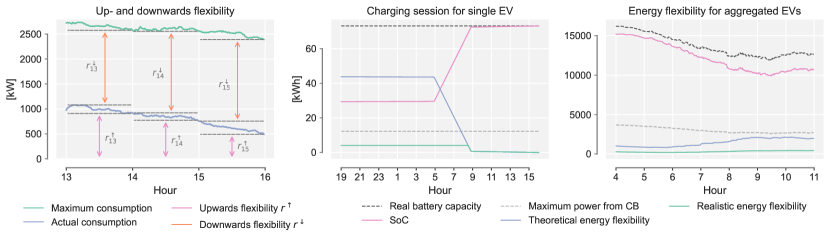
Figure 1: Illustrative examples of flexibility estimation: The figure on the left illustrates how downwards and upwards flexibility for the aggregated case are calculated. Downwards flexibility ($r^{\downarrow}$) is determined as the difference between the lowest point of the maximum consumption of the EVs and the highest actual consumption across the hour, while upwards flexibility ($r^{\uparrow}$) is the minimum of the actual consumption values during the hour. The middle and right figures show how energy flexibility ($r^{\rm{\rm{E_{20}}}}$) is calculated for a single EV and for the aggregated case. The single EV case represents a complete charging session, while the aggregated case captures a time interval in the day with large fluctuations in available flexibility, typically during the morning when many charging sessions end. Energy flexibility is calculated based on the current state of charge (SoC) and the amount of power that can be applied to the EV over the next 20 minutes without exceeding the battery’s capacity. For instance, at hour 1 in the single EV case, the SoC is 30 kWh, and the battery capacity is 75 kWh, meaning that, theoretically, the charge box (CB) could apply a maximum of 45 kWh in the next 20 minutes to fully charge the EV. However, due to the CB’s physical constraint of 12 kW, the actual available energy flexibility is much lower. Similarly, in the aggregated case, the theoretical and realistic energy flexibilities are on vastly different scales, reflecting the system’s capacity and constraints.

II-A FCR-D Market

Frequency containment reserve (FCR) is a category of ancillary services that helps balance short-term deviations in power and maintain the frequency stability of the electrical grid. In the Nordic grid, known for its low inertia, relatively small system size, and high share of stochastic renewable energy, FCR is divided into multiple services. These include FCR for normal operation (FCR-N), which is activated when the frequency deviates between 49.9 Hz and 50.1 Hz, and FCR for disturbances (FCR-D), which is activated when frequency deviations exceed the normal operational range. Specifically, FCR-D up services are triggered when the frequency drops below 49.9 Hz, while FCR-D down services are activated when the frequency rises above 50.1 Hz. To stabilize the grid, FCR-N and FCR-D service providers adjust their power production or consumption levels in response to frequency fluctuations. FCR-N is a symmetrical product, with equal bids made in both directions, whereas FCR-D is asymmetrical and split into two separate products: upward and downward [2]. FCR-N and FCR-D are procured in two distinct markets, each tailored to their specific operational roles. Without loss of generality, this paper focuses on the FCR-D market, as asymmetrical bidding for upward and downward services is well suited for EV aggregators and their battery state-of-charge constraints.

II-B The P90 Requirement

To maintain grid stability, the provision of ancillary services must be highly reliable. However, requiring a 100% reliability for ancillary service bids would restrict participation from many non-conventional technologies, such as wind power or aggregated flexible loads like EVs. To enable stochastic flexible resources to participate in the FCR markets, including FCR-D which is the focus of this paper, Energinet has introduced the P90 requirement, as outlined in [2] and [5].

The P90 requirement imposes that flexibility providers, such as EV aggregators, can participate in the FCR markets, provided that their reserved capacity bid is fully realized at least 90% of the time. A flexibility provider, after being qualified by the TSO, can participate in the relevant ancillary service markets, from which point Energinet will continuously check ex-post whether a reservation capacity bid by the participant truly exists or not. This is done no matter if the reserve is activated, as an extra measure of security of supply. For example, an upwards reserve bid of 10 kW will be seen as unavailable if the true consumption realization of an EV aggregator is 8 kW only. An unavailable bid, partially or fully, counts as a reserve shortfall. Energinet conducts these checks at appropriate time intervals, e.g., every quarter, and in the case of violation of the P90 requirement, the provider will be excluded from further participation in the market and must re-apply for the qualification. This requirement can be expressed mathematically using chance constraints of the form $\mathbb{P}(\cdot)\geq 1-\varepsilon$, where $\varepsilon$ represents the maximum 10% allowance for failure in successfully delivering the service.

II-C The LER Requirement

In addition to the P90 requirement, Energinet has imposed an additional requirement for resources with limited energy reservoirs (LER), such as batteries and EV aggregators. The primary focus of LER requirements is to ensure that resources with limited energy capacity can maintain energy availability despite their limitations. This includes adhering to energy management protocols and ensuring the ability to provide continuous activation for a certain minimum time duration when needed. The definition of this requirement is outlined in [2] and [5].

The specifics of the LER requirement vary between the FCR-N and FCR-D services. Focusing on FCR-D services in this paper, the requirement imposes that for an LER unit, when bidding in one direction of the FCR-D market (either up or down), at least 20% of the reserve bid must also be available in the opposite direction. For EV aggregators, this LER requirement applies only in the downwards direction, as the activation (i.e., increasing power consumption) is constrained by the battery energy storage capacity of EVs. In contrast, activation in the upwards direction (i.e., reducing power consumption) is not constrained by the battery capacity and is treated similarly to other non-LER flexible loads. Additionally, the requirement mandates that the service should be available for at least 20 continuous minutes once activated. These conditions result in the following constraints on the upwards and downwards reserve capacity bids of the EV aggregator (in kW), denoted as $b^{\uparrow}$ and $b^{\downarrow}$, to be submitted to the FCR-D market:

$$0.2b^{\downarrow}+b^{\uparrow} \leq R^{\uparrow},$$ (1a)

$$b^{\downarrow} \leq R^{\downarrow},$$ (1b)

$$b^{\downarrow} \leq R^{\rm{E_{20}}},$$ (1c)

where $\{R^{\uparrow},R^{\downarrow},R^{\rm{E_{20}}}\}$ are the three random variables representing the available upwards, downwards, and energy flexibility, respectively. Downwards flexibility, $R^{\downarrow}$, refers to the potential for increasing consumption of the grid-connected EV fleet, while upwards flexibility $R^{\uparrow}$, refers to the potential for reducing consumption. In addition, energy flexibility, $R^{\rm{E_{20}}}$, is calculated based on the current state of charge of the entire EV fleet and the amount of power that can be applied to the fleet over the next 20 minutes without exceeding their battery capacity. The realizations of these random variables are denoted by $\{r^{\uparrow},r^{\downarrow},r^{\rm{E_{20}}}\}$. A thorough explanation of how these realizations are defined can be found in Appendix A, along with a description of the case study. For readers seeking a quicker overview, Fig. 1 provides graphical representations of how the flexibilities are estimated. Specifically, the realizations $\{r^{\uparrow},r^{\downarrow},r^{\rm{E_{20}}}\}$ are defined as the extreme values of flexibility within the hour, which in our case corresponds to the minimum available flexibility during the hour. This approach contrasts with [5], where similar sets are defined using minute-level realizations. By taking the minimum value over the entire hour, we reduce the computational burden, as the number of data points is decreased by a factor of 60.

III Chance-Constrained Bidding Model

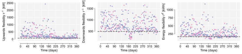
Figure 2: Scatter plots illustrating the estimated upwards (left), downwards (middle), and energy (right) flexibilities for an arbitrary hour across each day of the year. The blue dots represent the in-sample data used for optimization in a given run, while the pink dots are used for the ex-post out-of-sample validation in the same run. The dashed grey line indicates the 10^th percentile of the blue dots. In line with extreme value theory, only the samples below this percentile are used for estimation in the analytical method.

To incorporate the requirements imposed by Energinet into the bidding strategy, we use chance-constrained optimization. This approach handles uncertainty by ensuring that certain constraints are satisfied with a specified probability, rather than with absolute certainty. For EV aggregators participating in ancillary service markets, chance constraints allow them to make bids that balance reliability and resource utilization. Specifically, Energinet’s grid code requires that aggregators commit to a service provision that is fully available at least 90% of the time, allowing for a 10% margin of non-compliance due to uncertainties in EV availability.

Following the P90 and LER requirements, we adopt a joint chance-constrained optimization model similar to the one proposed in [5]:

$$\max_{b^{\downarrow},b^{\uparrow}\geq 0}b^{\uparrow}+b^{\downarrow}$$ (2a)

s.t.

$$\mathbb{P}\left(\begin{aligned} &0.2b^{\downarrow}+b^{\uparrow}\leq R^{\uparrow}\\ &b^{\downarrow}\leq R^{\downarrow}\\ &b^{\downarrow}\leq R^{\rm{E_{20}}}\end{aligned}\right)\geq 1-\varepsilon,$$ (2b)

where the objective function (2a) maximizes the combined reserve capacity bids into the FCR-D up and down markets. Additionally, (2b) defines the joint chance constraint that incorporates both the LER and P90 requirements. Specifically, the chance constraint $\mathbb{P}(\cdot)\geq 1-\varepsilon$ ensures that the probability of jointly satisfying the constraints within the corresponding hour is at least $1-\varepsilon$. According to the P90 requirement, $\varepsilon=0.1$.

Chance-constrained programs are generally computationally intractable. However, if the underlying probability distribution has certain properties, analytical reformulations of the chance constraints can be developed. For example, analytical methods like the Bonferroni approximation [14] transform probabilistic constraints into a series of more tractable constraints, simplifying the problem at the potential cost of precision. Alternatively, sample-based methods represent uncertainty through a set of likely scenarios, allowing for optimization that accounts for a range of possible outcomes. These approaches enable EV aggregators to optimize their bidding strategies while managing the stochastic nature of their resources within the operational constraints of ancillary service markets.

In Fig. 2 scatter plots of the in-sample and out-of-sample data used in our case study are shown. In-sample data refers to the set used in the optimization problem to determine optimal bids, while out-of-sample data is used ex-post for bid evaluation. Extreme value theory [15] focuses on the behavior of extreme values (maxima or minima) within a dataset, particularly as the sample size increases. We are especially interested in the extreme values, which in our case correspond to those below the dotted line in Fig. 2, representing the empirical 10^th percentile of the in-sample data. To avoid bias, we solve the model in multiple runs, each with different sets of in-sample and out-of-sample data, while keeping the number of samples in each set unchanged.

To derive an analytical solution to (2), we aim to fit a distribution to the tail data (samples below the empirical 10^th percentile) that allows for an analytical reformulation of the chance constraint. Among the various options for modeling tail data, we tested both the Weibull and Generalized Pareto distributions. We observed comparatively better out-of-sample performance when fitting the Weibull distribution.

It is worth noting that in the literature on extreme value theory, the Generalized Extreme Value (GEV) distribution is more commonly used as it emerges as the limiting distribution of the maximum of $n$ independent and identically distributed random variables when $n$ grows large. However, the convergence to this limit law may be poor. In addition, the GEV distribution introduces additional parameters that require tuning, which also may require more samples.

IV Distribution Fitting and Validation

This section outlines the methodology for fitting a probability distribution to our data, providing the necessary input for the analytical solution presented in Section V.

IV-A Fitting a Weibull Distribution to the Tail Data

Aiming to obtain an analytical solution, we fit a Weibull distribution to the tails of our data. The rationale for choosing this distribution lies in its flexible shape parameters, allowing to capture a wide range of tail behaviors. This flexibility is particularly advantageous, as this distribution can effectively model both skewed and heavy-tailed data. Its ability to adapt to both light and heavy tails enables us to accurately capture the realistic variability and potential extremes in the data.

The Weibull distribution has extensive applications in fields such as reliability engineering, where it models failure times and lifetimes, and in risk management for assessing minimum extreme events.

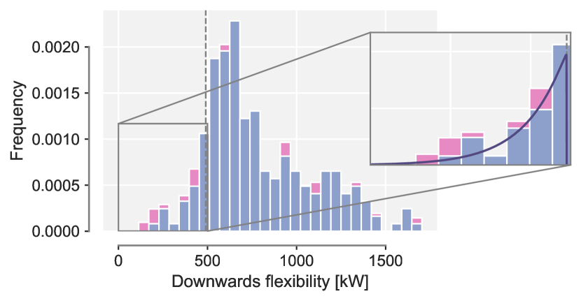
Figure 3: Distribution of the downwards flexibility at the arbitrarily selected hour 13. The blue distribution is constructed using in-sample data, while the pink part represents the out-of-sample data. A Weibull distribution with the shape parameter $\hat{\gamma}=0.9265$ is fitted to the lower tail of the blue distribution. The vertical dotted line indicates the 10^th percentile value of the in-sample data, below which the Weibull distribution is fitted.

For each flexibility $\{R^{\uparrow},R^{\downarrow},R^{\rm{E_{20}}}\}$, we select a subset of realizations for each hour for which we fit a distribution to the tail. As illustrated in Fig. 2, the relevant tail, in line with the case study and the P90 requirement, consists of all data points below the 10^th percentile, $r\leq r_{\varepsilon}=r_{0.1}$, where we let $r$ denote a realization of an arbitrary flexibility. Since the data in this tail does not resemble a Weibull distribution, we transform the data using $x=-r+r_{0.1}$, to which the Weibull distribution is more appropriately fitted. Fig. 3 illustrates the distribution of realizations of the estimated downwards flexibility, $r^{\downarrow}$, at hour 13. In line with Fig. 2, the blue bars represent the distribution based on in-sample data, while the pink bars correspond to the remaining out-of-sample data. We aim to fit a distribution based on the in-sample data. The threshold of the in-sample distribution, below which the Weibull distribution is fitted, i.e., the 10^th percentile of the sampled realizations, is indicated by a vertical dotted line.

We begin the procedure of fitting the Weibull distribution [16] by defining its two-parameter probability density function (PDF) as follows:

$$f(x) =\begin{cases}\kappa\gamma x^{\gamma-1}\exp(-\kappa x^{\gamma}),&x\geq 0,\\ 0,&x<0,\end{cases}$$ (3a)

where the scale and shape parameters, $$\kappa,\gamma>0 x\geq 0$$, can be estimated by maximum likelihood techniques. The likelihood function of (3a) is defined for as:

$$\mathcal{L}(x;\kappa,\gamma)=\prod_{i=1}^{n}\kappa\gamma x_{i}^{\gamma-1}\exp(-\kappa x_{i}^{\gamma}),$$ (3b)

where $$n \kappa \gamma \kappa \gamma$$ is the number of samples used for the estimation. Taking the logarithm of the likelihood function, then differentiating with respect to and in turn, and setting the derivatives equal to zero, we obtain the maximum likelihood estimator for in terms of the estimator of as:

$$\quad\quad\hat{\kappa}(\hat{\gamma})=\frac{n}{\sum_{i=1}^{n}x_{i}^{\hat{\gamma}}},$$ (3c)

where every symbol with a hat denotes the estimator of the corresponding variable. Substituting (3c) into the log-likelihood function, we obtain:

$$\ell_{n}(x;\hat{\kappa}(\hat{\gamma}),\hat{\gamma}) =n\left(\log n-\log\left(\sum_{i}x_{i}^{\hat{\gamma}}\right)+\log\hat{\gamma}-1\right)+$$

$$\quad\quad\quad\quad(\hat{\gamma}-1)\sum_{i}\log x_{i}^{\hat{\gamma}},$$ (3d)

which we maximize over a range of $\gamma$-values. Looking back at Fig. 3, the Weibull distribution is fitted to the lower tail of the sampled data, with the shape parameter $\hat{\gamma}=0.9265$.

As we will require later, we also define the cumulative distribution function (CDF) of the Weibull distribution as:

$$F(x) =\begin{cases}1-\exp(-\kappa x^{\gamma}),&x\geq 0,\\ 0,&x<0.\end{cases}$$ (4a)

We also define the tail distribution function, otherwise known as the survival function:

$$\bar{F}(x)=1- F(x)=\begin{cases}\exp(-\kappa x^{\gamma}),&x\geq 0,\\ 0,&x<0.\end{cases}$$ (4b)

IV-B Validation of Distribution Fits

To validate whether the fitted distribution correctly reflects the data, we use the Kolmogorov-Smirnov (KS) test [17]. This is a nonparametric test used to compare the equality of continuous, one-dimensional probability distributions, and it tests whether a sample comes from a specified reference distribution. The test statistic reports the maximum absolute difference between the empirical CDF, $F_{n}(x)$, and the reference CDF, $F(x)$, as:

$$D_{n}=\sup_{x}|F_{n}(x)-F(x)|,$$ (5)

where the empirical CDF is defined as

$$F_{n}(x)={\frac{1}{n}}\sum_{i=1}^{n}\mathbf{1}_{X_{i}\leq x}.$$ (6)

As before, $n$ represents the number of samples included in the estimation. Using (5), we can assess whether to reject or accept the hypothesis that the realizations come from the reference distribution through hypothesis testing. In this context, the null hypothesis $H_{0}$ assumes that the data comes from the specified reference distribution, while the alternative hypothesis $H_{1}$ assumes that it does not.

The KS test calculates the $D_{n}$ statistic and compares it to a critical value or uses it to compute a $p$-value based on the sample size and the reference distribution. If the $D_{n}$ statistic exceeds the critical value or the $p$-value falls below a pre-specified significance level (e.g., 0.05), $H_{0}$ is rejected, suggesting that the data is unlikely to come from the reference distribution. Otherwise, there is insufficient evidence to reject $H_{0}$, meaning the data is consistent with the specified distribution. This makes the KS test a robust tool for validating the goodness-of-fit between a dataset and a proposed model.

To further compare the goodness-of-fit between several distributions, such as the fit of the Weibull distribution for a range of parameter values, the negative log-likelihood (NLL) value is utilized, where a lower value signifies a better fit. This is because the NLL effectively quantifies how well a given model and its parameters explain the observed data, with lower NLL values corresponding to higher likelihoods of the observed data under the model. In essence, we use the negative of (3d) and compare the resulting value from a range of $\gamma$-values, and choose the $\gamma$ which gives us the lowest [18]. By using the NLL and the KS test, we validate that the obtained distribution fits are satisfying for our analysis.

V Analytical solution

This section presents the proposed analytical solution for addressing the chance-constrained bidding problem introduced in Section III.

V-A Bonferroni Correction

The joint chance constraint in (2) can be decomposed into three individual constraints using the Bonferroni correction [14]. This adjustment redistributes the overall allowance for violation equally across each constraint, effectively lowering the significance level for each test to ensure that the total probability of violation remains within the desired limit:

$$\mathbb{P} \left(R^{\uparrow}\leq 0.2b^{\downarrow}+b^{\uparrow}\right)\leq\frac{\varepsilon}{3},$$ (7a)

$$\mathbb{P} \left(R^{\downarrow}\leq b^{\downarrow}\right)\leq\frac{\varepsilon}{3},$$ (7b)

$$\mathbb{P} \left(R^{\rm{E_{20}}}\leq b^{\downarrow}\right)\leq\frac{\varepsilon}{3}.$$ (7c)

We conceptualize the method using hypothesis testing. The Bonferroni correction establishes an upper bound on the overall risk of incorrectly rejecting at least one hypothesis from the entire set being tested. The bound is valid regardless of any relationships between the hypotheses, but it is often larger than the true error probability. Specifically, for testing three hypotheses at a significance level $\varepsilon$, each hypothesis is rejected if its individual error probability is less than $\varepsilon/3$. The technique also accounts for data dependencies, despite its inherently conservative nature.

V-B Analytical Reformulation of the Optimization Problem (2)

Following the procedure in Section IV, the Weibull distribution is fitted to data under a threshold level, $r_{0.1}$, which in the present case is the empirical 10^th percentile of each flexibility, i.e., $\mathbb{P}(R\leq r_{0.1})=\varepsilon$. Applying Bayes’ theorem, we can thus express the conditional probability for an arbitrary random variable $R$ being under a certain threshold $b$ as:

$$\begin{split}&\mathbb{P}\left(R\leq b\mid R\leq r_{0.1}\right)=\mathbb{P}\left(R\leq b\right)/\mathbb{P}\left(R\leq r_{0.1}\right)\\ \Rightarrow&\mathbb{P}\left(R\leq b\right)=\mathbb{P}\left(R\leq r_{0.1}\right)\mathbb{P}\left(R\leq b\mid R\leq r_{0.1}\right),\end{split}$$ (8)

which gives a general formulation of the corrected constraints (7) as:

$$\varepsilon\mathbb{P}\left(R\leq b\mid R\leq r_{0.1}\right)\leq\frac{\varepsilon}{3},$$ (9)

which, after inserting the tail of the CDF in (4b), simplifies to:

$$b\leq r_{0.1}-\left(\frac{1}{\kappa}\log 3\right)^{1/\gamma}.$$ (10)

Using this formulation, with separately fitted distributions for each of the three flexibilities following the procedure outlined above, and applying the Bonferroni correction, the optimization problem (2) can be rewritten as:

$$\max_{b^{\downarrow},b^{\uparrow}\geq 0}b^{\uparrow}+b^{\downarrow}$$ (11a)

s.t.

$$0.2b^{\downarrow}+b^{\uparrow}\leq r_{0.1}^{\uparrow}-\left(\frac{1}{\kappa^{\uparrow}}\log 3\right)^{1/\gamma^{\uparrow}}$$ (11b)

$$b^{\downarrow}\leq r_{0.1}^{\downarrow}-\left(\frac{1}{\kappa^{\downarrow}}\log 3\right)^{1/\gamma^{\downarrow}}$$ (11c)

$$b^{\downarrow}\leq r_{0.1}^{\rm{E_{20}}}-\left(\frac{1}{\kappa^{\rm{E}}}\log 3\right)^{1/\gamma^{\rm{E}}},$$ (11d)

where the two latter constraints can be combined as $b^{\downarrow}\leq\min\{\eqref{eq:bonferroni opt prob CC2},\eqref{eq:bonferroni opt prob CC3}\}$. Using the correction method, the feasible region of the original problem (2) is reduced, meaning that any solution satisfying (11) will also satisfy (2). The optimization problem (11) is two-dimensional with linear constraints, and can be easily solved analytically. Fig. 4 provides a graphical representation of the optimization problem for the arbitrarily selected hour 1, illustrating how the optimal solution is found geometrically.

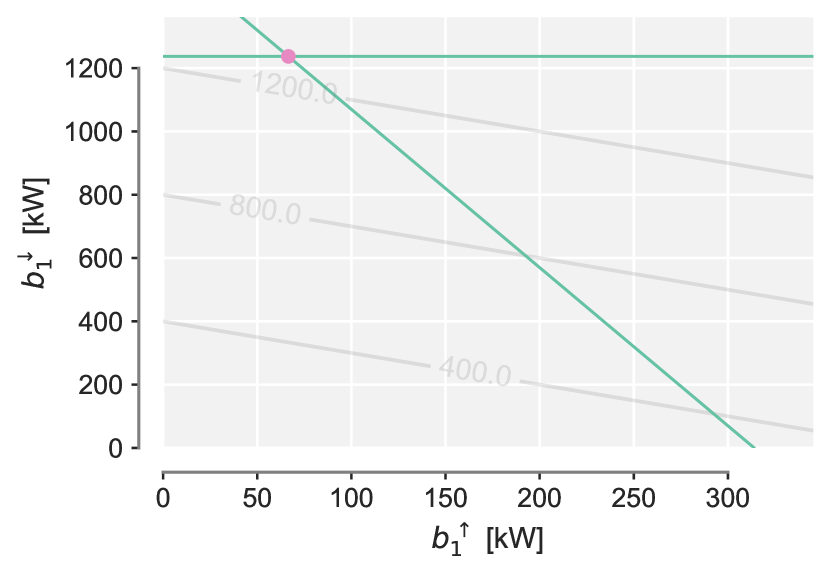
Figure 4: Geometric illustration of the optimization problem (11) for the arbitrarily selected hour 1. The grey lines are the contours of the objective function, and the green lines are the constraints, where the two constraints on $b^{\downarrow}$, (11c) and (11d), are combined into a single constraint as the minimum of the two, i.e., $b^{\downarrow}\leq\min\{\eqref{eq:bonferroni opt prob CC2},\eqref{eq:bonferroni opt prob CC3}\}$. The point where the green lines intersect indicates the optimal solution.

VI Sample-based solution for benchmarking

As a benchmark for our proposed analytical approach, we use the commonly adopted sample-based solution to reformulate (2).

VI-A Sample-based Reformulation of the Optimization Problem

We reformulate the joint chance-constrained optimization problem (2) using $|\Omega|$ samples, where each sample $i$ includes the realizations of the three random variables $\{r_{i}^{\uparrow},r_{i}^{\downarrow},r_{i}^{\rm{E_{20}}}\}$. This reformulation is written as:

$$\max_{b^{\downarrow},b^{\uparrow}\geq 0}b^{\uparrow}+b^{\downarrow}$$ (12a)

s.t.

$$0.2b^{\downarrow}+b^{\uparrow}-r^{\uparrow}_{i}\leq M^{\uparrow}y_{i},\quad i=1,\dots,|\Omega|$$ (12b)

$$b^{\downarrow}-r^{\downarrow}_{i}\leq M^{\downarrow}y_{i},\quad i=1,\dots,|\Omega|$$ (12c)

$$b^{\downarrow}-r^{\rm{E_{20}}}_{i}\leq M^{\rm{E_{20}}}y_{i},\quad i=1,\dots,|\Omega|$$ (12d)

$$\sum_{i=1}^{|\Omega|}y_{i}\leq|\Omega|\varepsilon,$$ (12e)

$$y_{i}\in\{0,1\},\quad i=1,\dots,|\Omega|,$$ (12f)

where $\{M^{\uparrow},M^{\downarrow},M^{\rm{E_{20}}}\}$ are sufficiently large positive constants, and $y_{i}$ is an auxiliary binary variable corresponding to sample $i$. Constraints (12b)-(12d) ensure that if $y_{i}=0$, all constraints are fulfilled for a specific sample $i$, while if $y_{i}=1$, these constraints are relaxed. Constraint (12e) ensures that the total budget for constraint violations is preserved, allowing for at most a 10% violation of the samples, in accordance with the P90 requirement. Due to the reduced number of data points in the case study, the problem remains tractable and can be solved without the need for additional relaxation.

VI-B Sampling

To find the minimum number of randomly selected samples necessary to accurately represent the estimated data, the following formula is used[19]:

$$|\Omega|\geq\frac{2}{\varepsilon}\log(\delta^{-1})+2p+\frac{2p}{\varepsilon}\log(2/\varepsilon),$$ (13)

where $p$ is the number of decision variables in the optimization problem (two in our case), $\varepsilon=0.1$ as per the P90 requirement, and by setting $\delta=0.01$, we achieve a 99% confidence level that the set of samples accurately represents the underlying distribution of the data. This results in $|\Omega|=216$ samples (approximately 60% of all realizations) being used for the optimization of bids across each hour, with the remaining 150 samples (approximately 40%) reserved for out-of-sample validation, as described in the following subsection.

VI-C Ex-post Out-of-sample Validation of Constraints

For the validation of the optimal reserve capacity bids obtained, i.e., $b^{\uparrow*}$ and $b^{\downarrow*}$, we construct a sample set $\Phi\notin\Omega$ and quantify the out-of-sample constraint violations. To do this, we count the number of instances where one or multiple of the following inequalities are violated for the realization of $\{r^{\uparrow}_{i},r^{\downarrow}_{i}$, $r^{\rm{E_{20}}}_{i}\}$, where $i=1,\dots,|\Phi|$:

$$0.2b^{\downarrow*}+b^{\uparrow*}-r^{\uparrow}_{i}>0,$$ (14a)

$$b^{\downarrow*}-r^{\downarrow}_{i}>0,$$ (14b)

$$b^{\downarrow*}-r^{\rm{E_{20}}}_{i}>0.$$ (14c)

Any violation of (14) for a given realization is counted as a violation of the joint chance constraint (2b). If more than one of the inequalities is violated simultaneously, it is counted as a single violation.

VII Numerical Results

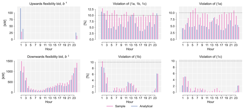
Figure 5: Illustrated in the leftmost plots are the bids for the upward and downward flexibility, respectively, using the two discussed methods: sample-based and analytical. The middle and right plots show the out-of-sample constraint violation rate, presented separately for each constraint and as an overall violation rate. All plots show the mean results obtained over 10 runs, with each run using different in-sample and out-of-sample sets, although the number of samples in each set per run remains unchanged.

In this section, we first present numerical results regarding the bidding strategy of the EV aggregator, obtained from both the analytical and sample-based solutions. We also report the rate of out-of-sample constraint violations and provide a sensitivity analysis with respect to $\varepsilon$. All source codes are publicly available in [20].

VII-A Bidding Strategy

A total of 10 simulations were run, where, following (13), $|\Omega|$ samples were randomly selected at each run and used for the procedures described in Sections V and VI. As a result, average reserve capacity bids over all runs into the FCR-D up and down markets are illustrated in the top and bottom left plots of Fig. 5. In the remaining plots, the average constraint violation rate is reported based on the out-of-sample validation procedure outlined in Section VI-C, using 40% of the samples not employed in the optimization procedure.

One of our main findings is that the analytical reformulation leads to fewer out-of-sample constraint violations compared to the sample-based approach in almost all cases. For instance, the decrease in constraint violation rate for hour 18 is 6.78%. This can be attributed to the higher bids made by the sample-based method, which compensates for the greater uncertainty associated with the sampled data. In addition to being more computationally tractable, the analytically formulated problem is also faster to solve, likely due to the significant reduction in the number of constraints. For instance, using 216 samples in the analysis results in approximately 680 constraints for the sample-based method. In contrast, the analytical method uses only 22 of the 216 samples for distribution fitting, and the optimization problem involves just three constraints.

We calculate the resulting revenue of the EV aggregator from offering ancillary services using historical FCR-D up and down prices in Denmark, defined as:

$$\sum_{h}b^{\uparrow*}_{h}\pi_{h}^{\uparrow}+b^{\downarrow*}_{h}\pi_{h}^{\downarrow},$$ (15)

where $\pi_{h}^{(\cdot)}$ represents the prices of the FCR-D capacity reservations, and $b^{(\cdot)*}_{h}$ is the bid made at hour $h$ in either direction. Using prices from the early auction of the FCR-D up and down markets from the relevant period, meaning the period spanning that of the collected data, and the results of the reserve bids, we obtain a reservation payment of €136,292 for the sample-based method and €105,366 for the analytical method when summing over the entire year. It is of relevance to extend the formula to include penalties for bid violations, to get a full picture of the profit of the aggregator, but that is outside the scope of this paper. However, reflecting on the results regarding constraint violation, there might be clues that the bids made by using the sample-based method may result in more penalties.

VII-B Sensitivity Analysis

For the sensitivity analysis, we focus solely on our proposed analytical approach.

It is of interest to study how the optimal reserve capacity bids change with varying values of $\varepsilon$, particularly how they might change when $\varepsilon$ becomes smaller, imposing a stricter requirement on reliability of the bids.

In (9), the allowance for failure is distributed across all requirements involved in the chance constraints. We can utilize this formulation to create a constraint that allows for a failure allowance lower than the level used in the distribution fitting scheme. Recall that we are using data from the lower 10^th percentile to fit distributions to each flexibility. This allows us to investigate whether we can find solutions to the bidding strategy with a violation allowance lower than 10%. To perform the sensitivity analysis on the failure allowance, we can define the constraints similarly to (11b)-(11d), replacing the right-hand side of (9) with an arbitrary $\alpha\in(0.0005,0.1]$, where $\alpha=0.1/3$ corresponds to the Bonferroni corrected problem. Following the same procedure as in Section V, we obtain the optimization problem for the bidding strategy:

$$\max_{b^{\downarrow},b^{\uparrow}\geq 0}b^{\uparrow}+b^{\downarrow}$$ (16a)

s.t.

$$0.2b^{\downarrow}+b^{\uparrow}\leq r_{0.1}^{\uparrow}-\left(-\frac{1}{\kappa^{\uparrow}}\log\left(\frac{\alpha}{\varepsilon}\right)\right)^{1/\gamma^{\uparrow}}$$ (16b)

$$b^{\downarrow}\leq r_{0.1}^{\downarrow}-\left(-\frac{1}{\kappa^{\downarrow}}\log\left(\frac{\alpha}{\varepsilon}\right)\right)^{1/\gamma^{\downarrow}}$$ (16c)

$$b^{\downarrow}\leq r_{0.1}^{\rm{E_{20}}}-\left(-\frac{1}{\kappa^{\rm{E}}}\log\left(\frac{\alpha}{\varepsilon}\right)\right)^{1/\gamma^{\rm{E}}}.$$ (16d)

Using this formulation, we can successfully obtain bids in both directions, with $\alpha$ potentially as low as 0.05% for some hours, depending on the underlying distributions. Following the sampling procedure (13) with the current sample set, we would not be able to reduce the constraint violation allowance to less than 6% [21] following the sample-based method, which represents a reduction of only 4%. This highlights the advantage of the analytical reformulation in this type of analysis.

Fig. 6 illustrates the total bids across 24 hours as a function of $\alpha$, as defined in (16), where $\alpha=0.02$ is the lowest value for which we could obtain bids for all 24 hours of the day. The bids shown are averages across 10 runs, similar to the results in Fig. 5. The point-wise 95% confidence level is indicated by a grey band, which is calculated in the standard way using the $t$-distribution [22]:

$$CI_{0.95}=\Bigg{[}\bar{x}-t_{.025,9}\frac{s}{\sqrt{10}},\ \bar{x}+t_{.025,9}\frac{s}{\sqrt{10}}\Bigg{]},$$ (17)

where $\bar{x}$ and $s$ represent the sample mean and sample standard deviation, respectively, and $t_{.025,9}$ is the critical value from the $t$-distribution with 9 degrees of freedom ($df=10-1=9$) for a two-sided 95% confidence level.

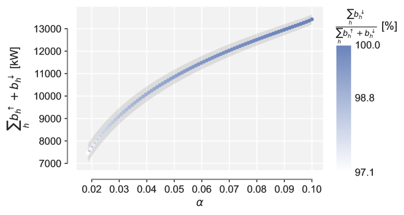
Figure 6: Total bids across 24 hours as a function of $\alpha$ in (16), where the dots denote the mean bids over 10 runs, and the gray band signifies the 95% confidence interval of the sample mean, calculated using (17). The dots are colored based on how much the bid in the downwards direction, $b^{\downarrow}$, covers the total bid in both directions.

VIII Conclusion and future work

Our findings highlight the effectiveness of the analytical model, derived from concepts of extreme value theory, compared to traditional sample-based methods. While sample-based approaches rely on large datasets to estimate constraints, they often face challenges such as high computational intensity and the potential underestimation of tail risks in rare, extreme market conditions—especially when the failure rate is very small. In contrast, our analytical approach requires fewer samples to reliably estimate the tail of the distribution, ensuring that probability constraints are accurately maintained even in low-probability, high-impact scenarios. This comparison demonstrates that the analytical approach not only reduces computational complexity but also better captures extreme fluctuations, ultimately enhancing both the accuracy and robustness of bids under market volatility. Our case study results illustrate this advantage: using the analytical reformulation, we obtained valid bids with violation rates as low as 0.05%, where the sample-based approach would have required nearly 85,000 samples, according to (13), to successfully place bids with this violation rate. Additionally, the analytical method, incorporating the Bonferroni correction, results in up to 7% fewer constraint violations, providing more reliable bids overall.

In future work, several approaches can further enhance the current study. One promising direction is dependency modeling with copulas to capture correlations between flexibilities, offering deeper insights and optimization strategies. Another opportunity lies in pooling data based on temporal factors, such as distinguishing between weekdays and weekends or accounting for seasonal variations, which could improve model accuracy by reflecting systematic patterns in EV energy consumption. We also suggest exploring dynamic reserve bidding, where strategies adapt in real-time to uncertainties like forecast errors or market fluctuations, to assess their impact on market efficiency and system reliability. Future work could also explore integrating ancillary service price forecasts or surrogate metrics like marginal opportunity costs to further refine the bidding strategy.

Appendix A Flexibility estimation

Our case study utilizes real-world data containing charging profiles from 1400 residential EV charging boxes (CB) in Denmark. The measurements are recorded from March 24, 2022, to March 21, 2023, with an average time-step of 2.84 minutes, which has been interpolated to obtain a one-minute resolution. It is assumed that only one EV is coupled with each CB. The historical EV consumption level serves as the baseline for the estimation of each flexibility.

The acquired data lacks user-specific information, such as the real battery capacity of the EV, the state of charge (SoC), and the maximum power rate of the CB, for which assumptions have been made to calculate them. To estimate flexibility, the data has been manipulated to include the following:

• $t$: index for time in minutes,

• $v$: index for EVs,

• $s$: index for charging sessions,

• $k_{v,t}$: a binary parameter indicating whether the EV $v$ is connected to the CB at minute $t$,

• $P_{v,t}$: instantaneous power output of the CB to the EV at minute $t$ [kW],

• $L_{v}$: battery capacity of the EV [kWh],

• $P_{v}^{\max}$: maximum power rate of the CB [kW],

• Current SoC [%], where it is assumed that the EVs battery is full (100%) when disconnecting from the CB.

We assume that the maximum battery capacity for every EV $v\in V$ is the largest energy output exerted by the CB over all charging sessions $s\in S_{v}$, where $S_{v}$ denotes the set of sessions for EV $v$. That is, $L_{v}^{\max}=\max\{\sum_{t}P_{v,t,s}\}$, $t\in[t_{s,0},t_{s}^{\max}]$, $t_{s,0}$ and $t_{s}^{\max}$ being the start and end time of charging session $s$. The SoC at each minute $t$ is given by $L_{v,t}=L_{v}^{\max}-(L_{v,s}-\sum_{i=1}^{t}P_{i,v})$, where $L_{v,s}$ is the total energy applied to the vehicle in the present charging session.

The energy that can be applied to the vehicle without exceeding the battery’s capacity is formulated as:

$$r^{\rm{E}}_{v,t}=(L^{\max}_{v}-L {}_{v,t})\prod_{i=t}^{t+20}k_{v,i},$$ (18a)

measured in kWh, where the product over $$k_{v,t}$$ ensures that the measure is only calculated if the vehicle is continuously connected to the CB in the next 20 minutes. To comply with the LER requirement, the constraint is restated:

$$r^{\rm{E}}_{v,t}\geq\frac{20}{60}r^{\downarrow}\quad \Rightarrow\quad 3r^{\rm{E}}_{v,t}\geq c^{\downarrow},$$ (18b)

where the unit of $$3r^{\rm{E}}_{v,t}$$ is in kW, signifying how much power the CB could theoretically output during the following 20 minutes. There is, however, a physical limit on the power output of the CB, and therefore the constraint is further restricted:

$$b^{\downarrow}\leq\min\{P {}^{\max}_{v,t},3r^{\rm{E}}_{v,t}\},$$ (18c)

that is, $r^{\rm{E_{20}}}_{v,t}=\min\{P^{\max}_{v,t},3r^{\rm{E}}_{v,t}\}$. In the case where the EV is not connected to the charger 20 minutes ahead, it will not have any energy flexibility unless it is considered in a portfolio where another CB can provide the flexibility.

The upwards flexibility, $r^{\uparrow}$, denotes how much the power applied to the EV can be reduced, and is simply defined as the power applied to the EV $v$ at the current time $t$ given that it is connected to a CB:

$$r^{\uparrow}_{v,t}= P_{v,t}k_{v,t}.$$ (19a)

On the other hand, the downwards flexibility, $$r^{\downarrow} P^{\max}_{v}=\max\{P_{v,t}\},t\in T_{v}$$, denotes how much the power applied to the EV by the CB can be increased, and is the maximum power rate the CB can provide, (all measured time for vehicle), minus the current power rate applied to the connected EV:

$$r^{\downarrow}_{v,t}=(P^{\max}_{v,t}- P_{v,t})k_{v,t}.$$ (19b)

Aggregation across vehicles for all flexibilities is simply calculated as the sum over all vehicles’ flexibility at each minute $$t$$:

$$r^{\rm{(\cdot)}}_{t}=\sum_{v} r^{\rm{(\cdot)}}_{v,t},$$ (19c)

where $$r^{\rm{(\cdot)}}\in\{r^{\uparrow},r^{\downarrow},r^{\rm{E_{20}}}\} h$$. As the reserve bid has to be uniform across each hour , the flexibility is bounded as the minimum available flexibility within the hour:

$$r^{\rm{(\cdot)}}_{h}=\min_{t\in[t_{0},t_{60})} \left\{r^{\rm{(\cdot)}}_{t}\right\},$$ (19d)

$t_{0}$ and $t_{60}$ being the start and end minute of hour $h$, respectively. Taking the minimum flexibility across the hour in this manner results in a loss of temporal dependencies in the data, which may lead to simplifications in the following analyses. The resulting data contains a year’s worth of flexibility for each hour of the day. Illustrative examples of how the flexibilities are calculated are found in Fig. 1. In Fig. 2 scatter plots of the (minimum) flexibilities for an arbitrary hour over the whole year are shown, where the horizontal line indicates the 10^th percentile, which serves as the threshold under which we are selecting data to use for our analysis in the analytical formulation of the bidding strategy.

References

- [1] Energinet (2024). “Ancillary services to be delivered in Denmark–tender conditions”, valid from October 2, 2024. [Online]. Available: https://en.energinet.dk/Electricity/Ancillary-Services/Tender-conditions-for-ancillary-services/
- [2] Energinet (2024). “Prequalification of units and aggregated portfolios”, version 2.1.2, valid from August 5, 2024. [Online]. Available: https://en.energinet.dk/electricity/ancillary-services/prequalification-and-test/
- [3] Lauinger, D., Vuille, F., Kuhn, D. (2024). “Reliable frequency regulation through vehicle-to-grid: Encoding legislation with robust constraints,” Manufacturing & Service Operations Management, vol. 26, no. 2, pp. 722–738.
- [4] Gade, P. A. V., Bindner, H. W., Kazempour, J. (2024). “Leveraging P90 requirement: Flexible resources bidding in Nordic ancillary service markets.” In the Proceedings of the IEEE SmartGridComm 2024 Conference, Oslo, Norway, pp. 1-6.
- [5] Lunde, G. A., Damm, E. V., Gade, P. A. V., Kazempour, J. (2024). “Aggregator of electric vehicles bidding in Nordic FCR-D markets: A chance-constrained program.” http://arxiv.org/abs/2404.12818
- [6] Blanchet, J., Jorritsma, J., Zwart, B. (2024). “Optimization under rare events: scaling laws for linear chance-constrained programs.” [Online]. Available: http://arxiv.org/abs/2407.11825
- [7] Nemirovski, A., Shapiro, A. (2006). “Scenario Approximations of Chance Constraints.” In: Calafiore, G., Dabbene, F. (eds) Probabilistic and Randomized Methods for Design under Uncertainty. Springer, London.
- [8] Prékopa, A. (1970). “On Probabilistic Constrained Programming.” Princeton University Press, Princeton, NJ. pp. 113–138.
- [9] Bawa, V. S. (1973). “On chance constrained programming problems with joint constraints,” Management Science, vol. 19, no. 11, pp. 1326-1331.
- [10] Nemirovski, A. (2012). “On safe tractable approximations of chance constraints,” European Journal of Operational Research, vol. 219, no. 3, pp. 707-718.
- [11] Roald, L. A. (2016). “Optimization methods to manage uncertainty and risk in power systems operation.” PhD Dissertation, ETH Zurich. [Online]. Available: https://www.research-collection.ethz.ch/handle/20.500.11850/125636
- [12] Nemirovski, A., Shapiro, A. (2006). “Convex approximations of chance constrained programs,” SIAM Journal on Optimization, vol. 17, no. 4, pp. 969-996.
- [13] Tong, S., Subramanyam, A., Rao, V. (2022). “Optimization under rare chance constraints.” [Online]. Available: http://arxiv.org/abs/2011.06052
- [14] Haynes, W. (2013). “Bonferroni Correction.” In: Dubitzky, W., Wolkenhauer, O., Cho, KH., Yokota, H. (eds) Encyclopedia of Systems Biology. Springer, New York, NY.
- [15] Castillo, E. (1988) “Extreme Value Theory in Engineering.” Academic Press, San Diego.
- [16] Cohen, C. A. (1965). “Maximum likelihood distribution estimation in the Weibull based on complete and on censored samples,” Technometrics, vol. 7. no. 4, pp. 579-588.
- [17] Dodge, Y. (2008). “Kolmogorov–Smirnov Test.” In: The Concise Encyclopedia of Statistics. Springer, New York, NY.
- [18] Cam, L. L. (1990). “Maximum likelihood: An introduction,” International Statistical Review, vol. 58, no. 2, pp. 153-171.
- [19] Luedtke, J., Ahmed, S. (2008). “A sample approximation approach for optimization with probabilistic constraints,” SIAM Journal on Optimization, vol. 19, no. 2, pp. 674–699.
- [20] GitHub Repository (2024) [Online] Available at: https://github.com/torine-dtu/EV-bidding-EVT-2024
- [21] Calafiore, G. C., Campi, M. C. (2006). “The scenario approach to robust control design,” IEEE Transactions on Automatic Control, vol. 51, no. 5, pp. 742–753.
- [22] Devore, J. L., Berk, K. N. (2012). “Modern Mathematical Statistics with Applications.” Springer, New York, NY.