PaNDaS: Partial Non-rigid Deformations and interpolations of Human Body Surfaces

Abstract

Non-rigid shape deformations pose significant challenges, and most existing methods struggle to handle partial deformations effectively. We present Partial Non-rigid Deformations and interpolations of the human body Surfaces (PaNDAS), a new method to learn local and global deformations of 3D surface meshes by building on recent deep models. Unlike previous approaches, our method enables restricting deformations to specific parts of the shape in a versatile way and allows for mixing and combining various poses from the database, all while not requiring any optimization at inference time. We demonstrate that the proposed framework can be used to generate new shapes, interpolate between parts of shapes, and perform other shape manipulation tasks with state-of-the-art accuracy and greater locality across various types of human surface data. Code and data will be made available after the reviewing process.

Figure 1: We present PaNDAS: a learning based approach to learn local and global non-rigid deformations of triangular meshes applied to human body surfaces. By combining per-face learned features on a neutral pose mesh (in blue) with a global encoding of a deformed mesh (in red), we are able to generate partial deformations (in cyan) restricted to user-chosen regions. Notably, these partially deformed meshes can create new poses, not present in the dataset. This approach permits several applications such as mixing poses, the transfer of partial pose interpolations and localized shape statistics.

1 Introduction

Generating deformations between 3D human shapes, such as the body, face, and hands, is a cornerstone in human-centered computer vision and graphics, facilitating a broad range of applications such as animation, human movement modeling, and character generation. This problem can be generally defined as follows: how to compute a sequence of non-rigid deformations of a source shape so it ends up matching a target shape ? In the case of human body surfaces, something left unsaid is that these deformations and interpolations should correspond to natural human motions to avoid breaking physical plausibility. In this work, we aim to address a broader version of this deformation problem by also tackling partial deformations as shown in Fig. 1. More precisely, we focus on computing non-rigid deformations of selected parts of a source shape so it matches the corresponding parts of a target shape while preserving physical plausibility.
In recent years, the problem of computing interpolation between shapes has been addressed extensively. Proposed solutions use geometric regularization [34, 8], model directly the shape space [21, 16, 18, 2, 4] or, more recently, learn shape interpolation by regularizing neural networks [11, 12, 10]. However, most of these approaches are not designed to address the challenge of partial deformations and interpolations without a complex configuration. Our present work aims to improve the flexibility of the deformation and interpolation processes by using learned, localized, latent features to deform specific parts of a shape. We propose a novel neural method for Partial Non-rigid Deformations of Surfaces (PaNDaS) to compute local and global non-isometric deformations of triangular meshes. Instead of representing shapes as a single latent vector, we propose to learn both a global shape latent vector and a local point-wise latent representation. Those vectors are fed into a deformation generator to obtain the desired mesh. By acting on local point-wise features, our model can interpolate between two shapes and locally deform a shape by masking the parts we want to deform. As shown in Fig. 1, PaNDAS can deform specific parts of the whole human body but also fingers on a hand and user-selected parts of faces. Additionally, one can apply a mix-and-match strategy to create new poses and compute partial shape statistics, as shown in Fig. 9. With no additional prior, PaNDaS set a new state-of-the-art regarding partial deformations and interpolations of surface meshes.
We summarize the main contributions of this paper as: (i) A new, end-to-end, deep learning framework to generate localized, non-rigid deformations of surface meshes, described in Sec. 3 and Sec. 4.2; (ii) This method is the first to allow vertex-level partial deformations and interpolations without requiring any texture information. This is made possible through the manipulation of predicted deep features as shown by several experiments in Sec. 4.4; (iii) We propose several applications such as new pose generation, partial pose deformation transfer and a robust statistical model of shapes handling partial descriptions. These applications are detailed in Sec. 4.5.

2 Related work

2.1 Geometric methods for Shape interpolation

Shape deformations and shape interpolation are intricately linked as interpolations consist of finding a continuous path of deformations applied to a source shape to match a target shape. Several frameworks have been proposed to ensure that the deformations lie in a well-defined shape space [6, 4]. To effectively compute these deformations and approximate a shape geodesic, traditional geometric approaches solve an optimization problem to minimize the energy of deformation. The latter can be defined from the well-established As-Rigid-As-Possible (ARAP) [2, 34] energy to make deformations close to rotations on a local level, PriMo [8] to ensure local rigidity through a prism formed between pairs of surface triangles and their extrusions. Other approaches directly model shapes as points in a shape space, with proper Riemannian metrics, such as the As-Isometric-As-Possible [21], Square Root Normal Fields [20] or parameterized familiy of elastic metrics [23, 5, 17] with terms penalizing specific deformations such as bending or stretching. While their expressions are different, these energy quantities serve the same purpose which is to measure local distortions of the shape when deformed to ensure near-isometric interpolations. However, the induced optimization problem is highly non-convex and can fail dramatically when the initialization is far from the desired solution. To address this performance issue, some methods proposed numerical schemes that simplify the initialization [24] or reduce the search space [16]. However, while some of these approaches could be used for localized manipulations, they often require extensive trial and error to set up the correct constraints for satisfying results. In contrast, we designed our model to deal with both partial and local deformations with limited preprocessing steps.

2.2 Deep Learning Approaches for Shape Deformation

More recently, deep learning methods have been proposed to learn shape deformations. The most popular approach consists of building a latent space using an auto-encoder formulation. For this, graph convolutional auto-encoders can be used [13, 9, 42, 35, 36] however, they tend to overfit information from the input mesh connectivity. Other approaches such as 3DCODED [14] learn auto-encoders for shape matching [15, 28], but are not optimized for shape deformations, and tend to fail when the target deformation is highly non-linear. More recent deformation models such as Neural Jacobian Fields (NJF) [1] improve the generated deformations but are prone to produce non-physical results when unconstrained. To address this problem, other methods propose to regularize the latent space. The authors of LIMP [11] propose geometric penalties based on the preservation of geodesic distances to regularize the latent space. ArapReg [19] penalizes directions in the latent space that affects the ARAP energy, a strategy that has been improved to provide a geometric latent space [39] or to learn correspondences [40]. Other methods [12, 10] directly learn to produce interpolations between pairs of shape, but they can struggle with details and may fail to generalize to new data. All these methods focus on learning full shape deformations which limits applications such as partial shape interpolations. In this paper, we propose a method to overcome this limitation and allow the interpolation of parts of meshes extending the range of possible deformation sequences by a large margin.

2.3 Neural methods for Local and Partial Deformations

While optimization-based algorithms can be adapted to partial deformation, they usually require a custom configuration for each data category. A few learning based methods [25, 42] enable partial deformations and interpolations by structuring the latent space according to the initial shape structure. This allows the user to modify latent points that affect specific parts of the shape. However, as the relationship between latent points and mesh vertices is predefined before training, the level of detail of partial deformations remains limited. Recently, deep methods have started addressing localized control for images [38, 33]. While extending these to surface data is not straightforward because of the non-euclidean nature of shapes, several works leverage this idea for mesh deformations [37, 41], by combining image diffusion models prior with suitable deformation models such as Neural Jacobian fields [1] or by defining key points during movements [27]. However, those methods rely on additional information such as texture maps, user prompts for the diffusion model, or skeletal joints. They also require several optimization steps, making them impractical for applications in which these priors are unavailable.
To overcome this limitation, our method leverages a learned and controllable feature field paired with a deformation generator which predicts a constrained Jacobian field, used to generate partial, natural deformations of the mesh.

3 Description of our approach

In this section, we explain our approach for which a diagram is associated in Fig. 2. More details about the elements of the architecture and the training procedure can be found in the supplementary material.

3.1 Problem formulation

From a source mesh $\mathcal{X}=(x_{i})_{1\leq i\leq n_{\mathcal{X}}}$, with $n=n_{\mathcal{X}}$ vertices (the mesh of the ”neutral pose”), we wish to match a target mesh $\mathcal{Y}=(y_{i})_{1\leq i\leq n_{\mathcal{Y}}}$ with, $n_{\mathcal{Y}}$ vertices. To do so, we predict a deformation field $v=(v_{i})_{1\leq i\leq n}=(v^{\mathcal{X},\mathcal{Y}}_{i})_{1\leq i\leq n}$, that morphs $\mathcal{X}$ onto $\mathcal{Y}$. In the case of point-to-point correspondence, we would want to find

$$y_{i}=x_{i}+v_{i},\quad 1\leq i\leq n.$$ (1)

Our proposed framework to compute $v$ can be divided in 3 parts: a neutral pose feature extractor $Enc_{N}$, a deformation encoder $Enc_{D}$ and a deformation generator $Dec$. First, $Enc_{N}$ encodes the geometric information of $\mathcal{X}$ into a local feature vector $f_{t}\in\mathbb{R}^{l}$ for each triangle $t$ of the mesh $\mathcal{X}$, for a total of $l\times m$ features. Here, $m=m_{\mathcal{X}}$ the number of triangles in $\mathcal{X}$. Then, $Enc_{D}$ encodes both $\mathcal{Y}$ and $\mathcal{X}$ into a single global feature vector $z$. The local (triangle-wise) features $f_{t}$ and global features $z$ are combined to obtain a local feature vector $\tilde{f}_{t}=(f_{t},z)\in\mathbb{R}^{l+r}$ on each triangle $t$ of $\mathcal{X}$. The decoder then computes from $\tilde{f}$ a deformation field $(v_{i})_{1\leq i\leq n}$, along with the vertices $(x_{i}+v_{i})_{1\leq i\leq n}$ of $\hat{\mathcal{Y}}$, the deformed mesh. The locality of the latent code will allow for local manipulation to create new motions and partial interpolations.
We now describe in detail how each of those pieces works.

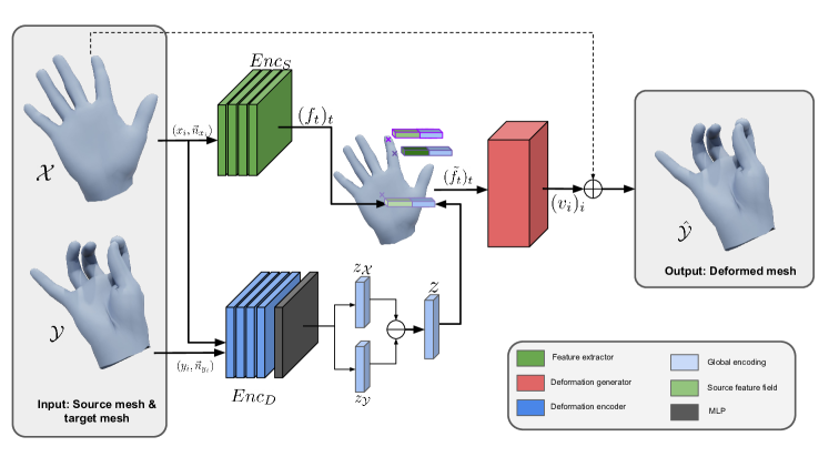
Figure 2: Overview of the proposed architecture. A pair of meshes is given as input: a source pose $\mathcal{X}$ and a target pose $\mathcal{Y}$. Per-triangle features $(f_{t})_{t}$ are learned on the source mesh and are enriched with a global encoding $z$ of the target mesh to obtain a feature field $(\tilde{f}_{t})_{t}$ over the source mesh. Finally, the deformation generator learns a Jacobian field from the feature field over the neutral mesh to predict a first-order, per-triangle displacement field $(v_{i})_{1\leq i\leq n_{\mathcal{X}}}$.

3.2 Neutral pose feature extractor

To compute local descriptors on $\mathcal{X}$, we employ 4 DiffusionNet [32] blocks as a face-wise feature extractor $Enc_{S}$ on the source mesh. Heat diffusion is used to a remeshing invariant convolutional neural network, and has proven its efficiency in computing local geometric features [3]. The encoder takes as input the neutral pose mesh $\mathcal{X}$ and outputs a feature vector $f_{t}\in\mathbb{R}^{l}$ of size $l=64$ for each triangle $t$ of $\mathcal{X}$. We slightly modify the original architecture by adding a Group Normalization (GN) module in the Multi Layer Perceptron (MLP), between the Linear layer and the ReLU activation.

3.3 Deformation encoder

Simultaneously, we train a global encoder of deformations $Enc_{D}$, also based on four DiffusionNet blocks. First, just like in the previous section, it predicts a feature vector $g_{t}$ on each triangle $t$ of $\mathcal{Y}$. Next, we aggregate this entire field of features into a single $r$-dimensional feature vector $z_{\mathcal{Y}}$. For this, we propose a novel aggregation operator at the end of the network. Denote $e^{k}$ the $k$-th eigenvector of the cotangent Laplacian $\Delta^{\mathcal{Y}}$ on the triangles of $\mathcal{Y}$. Do note that each $e^{k}_{t}$ is a scalar for each face $t$ (remark that $e^{1}_{t}$ is constant with respect to $t$, since constant functions belong to the kernel of $\Delta^{\mathcal{Y}}$). Now $g=(g_{t})_{t}$ can be decomposed as $g_{t}=p_{1}e^{1}_{t}+p_{2}e^{2}_{t}+\dots$, with each $p_{k}$ being a $r$-dimensional vector corresponding to the $k-$th frequency of $g$, computed through a weighted average so that

$$p_{k}=\frac{1}{\mathrm{Area}(\mathcal{Y})}\sum_{t=1}^{m_{\mathcal{Y}}}\mathrm{Area}(t)g_{t}e^{k}_{t}.$$ (2)

Here, $m_{\mathcal{Y}}$ denotes the number of faces in $\mathcal{Y}$, and $\mathrm{Area}(t)$ is the area of the $t$-th face of $\mathcal{Y}$. In particular, $p_{1}$ is just the area-weighted average of $g$. Next, we concatenate the first $s$ frequencies of these projections and pass this vector through a linear layer $Lin$ to obtain a global encoding $z_{\mathcal{Y}}\in\mathbb{R}^{r}$ of size $r=64$ of $\mathcal{Y}$. In our experiments, $s=4$ proved to be sufficient. Hence,

$Enc_{D}(\mathcal{Y})=z_{\mathcal{Y}}=Lin(p_{1},p_{2},p_{3},p_{4})$

is a single vector in $\mathbb{R}^{r}$. At the same time, this encoder also computes $z_{\mathcal{X}}=Enc_{D}(\mathcal{X})$ and the final latent vector of deformation is simply $z=z_{\mathcal{Y}}-z_{\mathcal{X}}$. In the particular case $\mathcal{X}=\mathcal{Y}$, we get $z=0$.
Now, we go back to $\mathcal{X}$ and $f=Enc_{N}(\mathcal{X})$ from the previous section. For every triangle $t$ of $\mathcal{X}$, append the feature $f_{t}$ with a copy of the global feature $z$. This gives the final learned feature field $Enc(\mathcal{X},\mathcal{Y})=\tilde{f}$, where each face $t$ of $\mathcal{X}$ carries the feature

$\tilde{f}_{t}=(\tilde{f}_{t,i})_{1\leq i\leq l+r}=(f_{t},z)\ \in\mathbb{R}^{l+r}.$

These features locally describe how a source mesh $\mathcal{X}$ should be deformed to match a target mesh $\mathcal{Y}$. The total number of features is $m_{\mathcal{X}}\times(l+r)$.

3.4 Deformation generator with Jacobian fields

From the predicted features put forward by the encoder, the deformation generator uses neural Jacobian Fields [1]: it learns per-face candidates for Jacobians matrices $(J_{t})_{1\leq t\leq m_{\mathcal{X}}}\in\mathbb{R}^{3\times 3}$ of the final deformation field $v$. Differing from the original paper, instead of attaching the triangle centroïds to a global encoding, we predict the Jacobian field directly from the predicted features $(\tilde{f}_{t})_{1\leq t\leq m_{\mathcal{X}}}$. Then, these Jacobians are restricted to their corresponding triangle. For notation simplification, we will keep $J_{t}$ to denote the restricted Jacobian. Hence, we have $v$ in $\mathbb{R}^{3\times n}$ (recall that $n$ is the number of vertices of $\mathcal{X}$) such that $J_{t}=\nabla_{t}v$ with $\nabla_{t}$ the gradient operator at triangle $t$. However, just like any vector field may not be a gradient, any such family of $J_{t}s$ may not be the Jacobian of a well-defined deformation. This is resolved when taking the closest match for $v$ by solving the Poisson equation $\nabla^{\mathcal{X}}v=\nabla^{T}\mathcal{M}J$, with $\mathcal{M}$ the mass matrix of the source mesh and $J$ the stack of per-face Jacobians $J_{t}$. Then, the decoder $Dec$ learns a displacement field $v$ on the template mesh $\mathcal{X}$ so that the model outputs the deformed mesh $\hat{\mathcal{Y}}$ with vertices $\hat{y}_{i}=x_{i}+v_{i}$, $i=1,\dots,n$:

$$Dec:\begin{cases}\mathbb{R}^{m_{\mathcal{X}}\times(l+r)}&\rightarrow\mathbb{R}^{n_{\mathcal{X}}\times 3}.\\ (\tilde{f}_{t})_{1\leq t\leq m}&\mapsto(v_{i})_{1\leq i\leq n}\end{cases}$$ (3)

3.5 Training strategy

The model is trained end-to-end by minimizing a training loss function $\mathcal{L}$ composed of a reconstruction loss $\mathcal{L}^{rec}$ and an additional term on the normal map $\mathcal{L}^{n}$drawn directly from the predicted Jacobians:

$$\mathcal{L}=\mathcal{L}^{rec}+\lambda^{n}\mathcal{L}^{n}$$ (4)

where $\lambda^{n}$ is a weighting factor.
By default, $\mathcal{X}$ and $\mathcal{Y}$ are aligned (there is a point-wise correspondence) but the different component of the model allows changes in the topology of the meshes. With registered data, we use the (Mean Squared Error) MSE for the reconstruction loss:

$$\mathcal{L}^{rec}(\mathcal{Y},\hat{\mathcal{Y}})=\frac{1}{n_{\mathcal{X}}}\sum_{i=1}^{n_{\mathcal{X}}}\left\|y_{i}-(x_{i}+v_{i})\right\|_{2}^{2}$$ (5)

Next, we use the normal map to regularize the feature field to obtain smoother deformations. To do so, from the restricted jacobians $J_{t}$ we extract a normal vector $\vec{n}_{t,\mathcal{Y}}$ as a cross product.

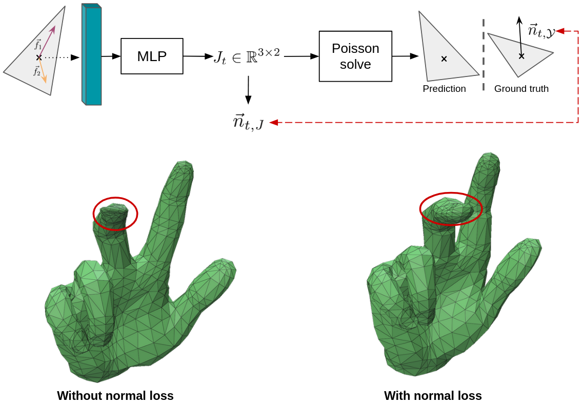
Figure 3: Qualitative comparisons of the regularization effect when adding a loss term on the normal map. On the bottom left is a generation mid-interpolation for a model trained only with the MSE loss, on the right is a similar generated mesh but with a model trained with a loss on the normal map.

This ”intermediate” normal vector will be changed after solving the Poisson equation. However, our experiments showed that using the one from the Jacobian (before the Poisson solve) enhances the quality of deformations from interpolated codes as shown in Fig. 3. Then, the loss on the normal map is the Cosine similarity between the target normals $\vec{n}_{t,J}$ and the predicted normals $\vec{n}_{t,J}$ at every triangle $t$:

$$\mathcal{L}^{n}(\mathcal{Y},\hat{\mathcal{Y}})=\frac{1}{m_{\mathcal{X}}}\sum_{t=1}^{m}[1-\vec{n}_{t,\mathcal{Y}}\cdot\vec{n}_{t,J}]$$ (6)

3.6 Interpolation, Partial Deformation, Mixing Deformations

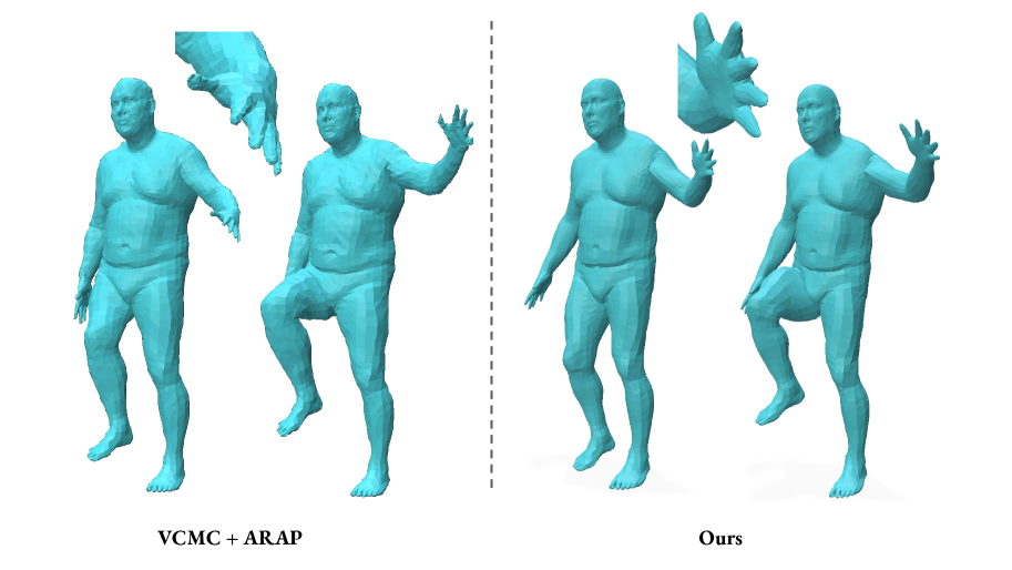
Figure 5: Pose mixing using partial interpolations of a neutral pose with two other poses. The first pose raises both arms (only the left one is used for interpolation).The second pose raises the right knee. We highlight how our method (on the right) compute smoother deformations and avoid limb shrinking (right leg on the left).

Once the model is trained, one can perform the usual operations in the latent space. For example, we get an interpolation between $\mathcal{X}$ and $\mathcal{Y}$ by decoding a linear interpolation at each triangle $t$ between $(f_{t},0)$ (the encoded features for $\mathcal{X}$) and $\tilde{f}_{t}=(f_{t},z)$ (the encoded features for $\mathcal{Y}$). But, the true value of PaNDaS comes from the intrinsic locality of the feature field $t\mapsto\tilde{f}_{t}=(f_{t},z)$ which can be leveraged to obtain completely new poses. To obtain partial deformations, one can multiply the $z$ part of the local features by a mask $\mathfrak{M}=(\mathfrak{M}_{t})_{1\leq t\leq m}\in\{0,1\}^{m}$, equal to either 1 or 0 on each triangle, to only deform parts of the surface: $\tilde{f}_{t}^{\mathrm{partial}}=(f_{t},\mathfrak{M}_{t}z)$. This gives a lot more flexibility than previous approaches [42] limited to latent points. We can then of course perform interpolation between the neutral pose and the partially deformed shape (see Fig. 1). More generally, we can take several global features $z^{1},\dots,z^{j}$ encoded from several poses $\mathcal{Y}^{1},\dots,\mathcal{Y}^{j}$, assign a part of the shape (and a corresponding mask) to each one and decode the feature field $\left(f_{t},\mathfrak{M}^{1}_{t}z^{1}+\dots+\mathfrak{M}^{j}_{t}z^{j}\right)_{1\leq t\leq m}$ to produce new deformations (see Fig. 5).

4 Numerical Experiments

We showcase the efficiency of our method with three different experiments: the first one compares the quality of the generated deformation obtained with the model inference. A second experiment compares the quality of deformation sequences obtained through linear interpolation of the feature field. Finally, a third experiment shows qualitative evaluation of partial interpolations.
Additionally, complex animations performed using the model can be found in the supplementary material videos.

4.1 Metrics and data

Datasets. We showcase the adaptability of our method with experiments on 3 different datasets.
MANO [30] is a dataset of hand meshes comprising 30 hand identities, each in around 20 poses. A registered version of the dataset is aligned to a fixed topology with 778 vertices and 1538 faces. We perform a prior Procrustes alignment [31] of the meshes.
DFAUST. [7] is a 4D dataset of 10 human subjects executing 13 different movements. The complete dataset is made of 40,000 meshes and we selected 20 meshes per movement from the first 100 frames of each sequence. Our training set is made 1140 meshes and the test set is made of 300 meshes.
COMA [29] is a face mesh dataset gathering 12 identities, executing 12 different (”extreme”) expressions. The full dataset contains more than 20,000 meshes and we uniformly sampled 2000 of them. We also removed the eyeballs which were separated connected components of the face mesh.
Metrics To evaluate mesh reconstructions on registered data, we use the MSE, the Hausdorff distance (HD) and chamfer distance (CD). Similarly, we evaluate latent interpolations against ground truth movements. For this, we employ the averaged frame-by-frame MSE and Chamfer distance.

4.2 Generating deformed mesh

In this experiment, for each identity in the dataset, we have an identified neutral pose mesh $\mathcal{X}$. Then, given a target mesh $\mathcal{Y}$, the model predicts a deformation field $v$ over $\mathcal{X}$. We observe and measure the quality of the predicted deformed mesh and its distance to the target mesh in Tab. 1. We compared our model with several deep learning methods: Neural Jacobian Fields (NJF) [1] proposed an auto-encoding approach to predict a point-wise deformation. Variant Coefficient MeshCNN (VCMC) [42] is a graph convolution method, LIMP [11] and ARAPReg [19] learns a regularized linear latent shape space of deformations to disentangle identities and poses. In this setting, PaNDaS surpasses the others for large non-linear deformation generations (on MANO and DFAUST) and comes at a close second for face expression deformations.

	MANO				DFAUST				COMA
	MSE $\downarrow$	HD $\downarrow$	CD ($10^{-5}$) $\downarrow$		MSE $\downarrow$	HD $\downarrow$	CD ($10^{-5}$) $\downarrow$		MSE $\downarrow$	HD $\downarrow$	CD ($10^{-5}$) $\downarrow$
LIMP [11]	-	0.049	71.9		-	0.141	0.0047		-	0.0095	1.021
VCMC [42]	0.2240	0.014	5.86		2.92	0.076	0.0017		0.191	0.01400	1.506
ARAPReg [19]	0.1986	0.009	3.29		2.61	0.069	0.0011		0.128	0.0070	0.474
NJF [1]	0.3019	0.019	9.65		5.01	0.126	0.0029		0.238	0.0105	1.435
Ours	0.1422	0.010	2.94		2.23	0.058	0.0009		0.160	0.0086	0.839

Table 1: Reconstruction errors of poses from a given identity. We evaluate the quality of the deformations using distances between the predicted deformed mesh and the target mesh.

4.3 Interpolation evaluation

Secondly, we also validate the quality of latent interpolation sequences using comparisons with short movements in DFAUST and COMA datasets. We report the MSE and mean chamfer distances of the generated sequences in Tab. 3 and Tab. 3 against ground truth movements. We compare the performances with other recent approaches relying on latent interpolation. ARAPReg [19] enables interpolation as a linear latent interpolation inducing a shape interpolation by decoding the sequence of latent vectors. Similarly, VCMC enable partial deformations through latent vertices on which latent interpolations are possible.

	MSE $\downarrow$			CD ($10^{-2}$) $\downarrow$
	VCMC	ARAPReg	ours	VCMC	ARAPReg	ours
punching	11.98	8.94	8.67	1.02	0.85	0.83
running	10.76	9.52	9.40	1.11	1.02	1.05
shake a.	16.48	10.98	10.28	2.56	1.73	1.63
chicken	14.82	9.17	9.03	1.21	0.90	0.84
knees	5.02	4.52	4.22	0.52	0.38	0.34
jumping	21.46	18.08	17.08	3.74	3.18	2.98
one leg j.	6.31	5.25	5.41	0.46	0.38	0.41
one leg l.	5.57	4.70	4.94	0.43	0.40	0.37
Mean	11.55	8.87	8.71	1.38	1.10	1.06

Table 2: Interpolation evaluation on DFAUST sequences.

	MSE $\downarrow$			CD ($10^{-5}$) $\downarrow$
	VCMC	ARAPReg	ours	VCMC	ARAPReg	ours
bareteeth	0.16	0.12	0.10	1.05	0.51	0.40
cheeks in	0.16	0.11	0.10	1.08	0.38	0.35
mouth up	0.15	0.10	0.08	0.93	0.41	0.34
high smile	0.15	0.09	0.10	0.96	0.35	0.37
lips back	0.17	0.12	0.11	1.15	0.44	0.39
lips up	0.16	0.08	0.09	0.92	0.22	0.26
mouth side	0.16	0.12	0.11	1.08	0.51	0.43
mouth ext.	0.22	0.13	0.13	1.46	0.52	0.51
Mean	0.17	0.11	0.10	1.08	0.42	0.38

Table 3: Interpolation evaluation on COMA sequences.

PaNDaS is competitive compared to these methods on both metrics. To support the quantitative evaluation, we also show qualitative displays of the interpolations in Fig. 10. More examples are given in the supplementary material.
For fair comparison, we excluded optimization algorithms and methods [16, 12, 10] that does not involve a learned latent representation of the deformation: Bare-ESA [16] solves a restricted optimization problem and Spectral Meets Spatial learns directly the deformation field in a joint spectral and spatial domain. It is worth noting that ARAPReg performs worse than on the reconstruction task primarily because of highly non linear deformation sequences (see Fig. 10). In fact, the ARAP regularization is efficient on deformation close to linear deformations.

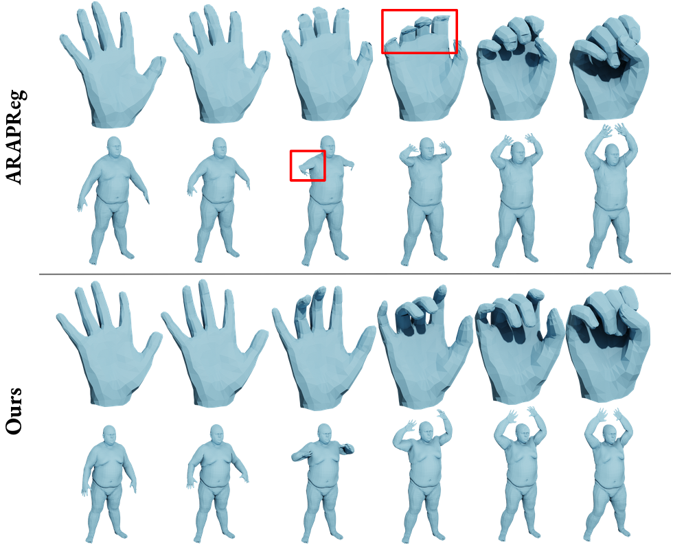
Figure 4: Pose interpolation example obtained using latent linear interpolation with ARAPReg (top row) compared to the same interpolations computed using PaNDaS (bottom row). The latter handles better large and highly non linear deformations.

4.4 Partial deformations and local manipulations

In this part, we experiment with partial deformations. Thanks to our training strategy, the generated deformations maintain a global smooth coherent mesh. In particular it enables the generation of new poses, unseen by the deformation generator. We compare the partial deformations with a localized As-Rigid-As-Possible (ARAP) vertex displacement. The implementation is heavily borrowed from [26]. Other methods such as DragD3D [37] and APAP [41] cannot be used for comparison as no texture map is available in our experiment. Results are presented in Fig. 6 and more qualitative examples can be found in the supplementary material.

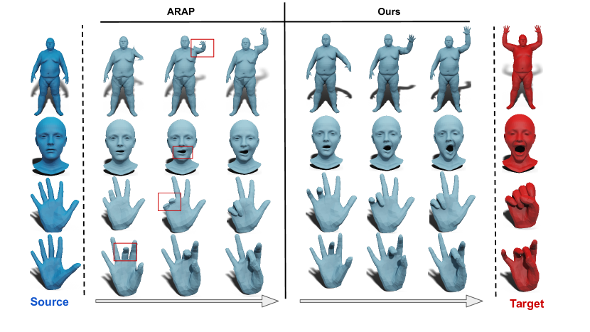
Figure 6: Qualitative comparisons of partial deformations on DFAUST, COMA and MANO. The As-Rigid-As-Possible deformations handles efficiently deformations that are close to linear (2nd and last row) but fails to adapt to large deviations.

We insist on the versatility of this method: from a limited collection of different poses, our model enables a large range of possible partial deformations and this deep features manipulation makes precise animation of articulated meshes possible. Notably, it does not require additional skeleton information to produce meaningful movements.

4.5 Applications: mixing and shape statistics

Deformation mixing.

As described in Section 3.6, PaNDaS can mix partial deformations on different shape parts. This is done through the use of chosen masks on the deep features corresponding to how we want to deform each part. We can then generate new poses as illustrated in Fig. 7.

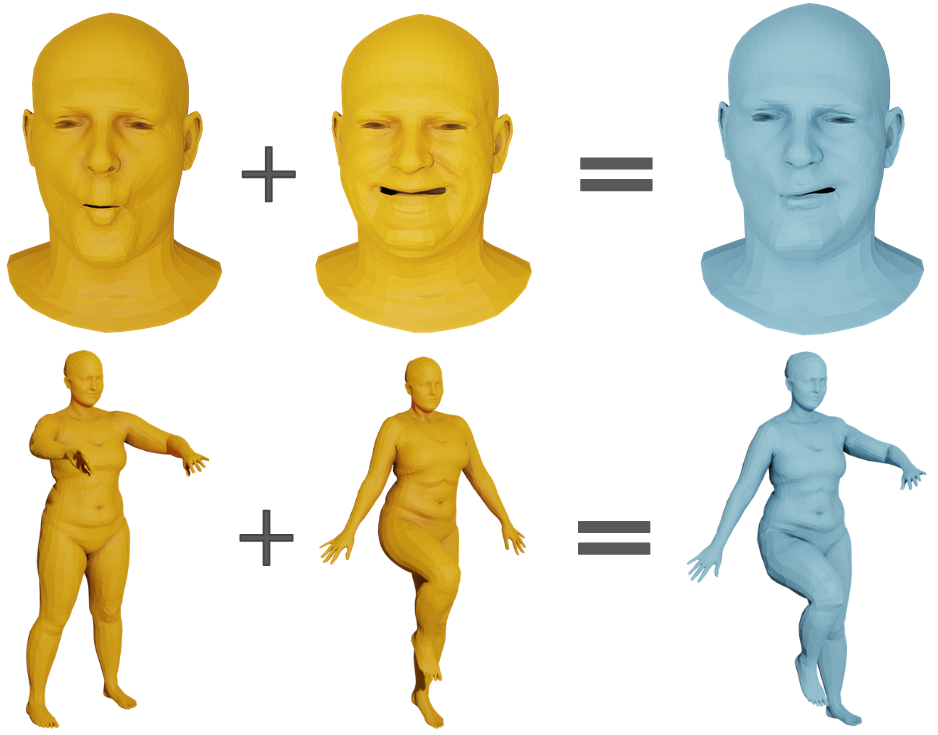
Figure 7: Mixing different poses (in yellow) and partial deformations to generate new poses (in blue).

A statistical model of deformations.

PaNDaS can be used to estimate the mean shape from a collection of given shapes and we display estimated means in Fig. 8. We show how our method gives more plausible results (on the right) than a linear mean computation (on the left).
In addition, because our PaNDaS relies on modules that are robust against remeshing: we show that the prediction handles scans with arbitrary mesh topology.

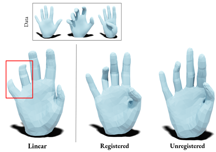
Figure 8: Mean shape of three hand poses. We compare the estimated mean in a registered setting and an unregistered setting with a linear mean. The mean produced using PaNDaS is a plausible hand compared to the linear mean (see highlights in red square).

Also, because our method handles partial deformations, it can compute partial means and principal components, as shown in Fig. 9. Interestingly, these components can be used to build a basis of controllable and localized movements.

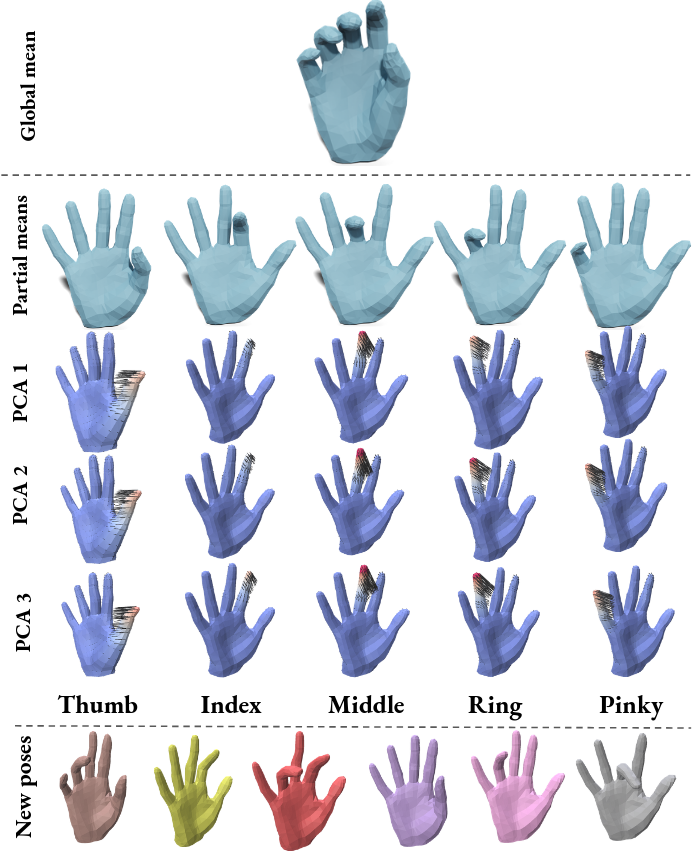
Figure 9: We compute partial statistics using local latent vectors on the MANO dataset. In addition, we use Principal Component Analysis (PCA) to capture the principal directions of deformation for each finger. In the figure, PCA X designates the deformation field predicted by using X principal component of the feature field. Notably, we can use this approach to generate new poses by combining components of each finger.

5 Limitations and future work

While PaNDaS architecture is invariant to mesh topology, as other state-of-the-art methods, it is trained with registered meshes. An exciting possibility of future work is to explore recent strategies for unregistered training [15, 40], to train PaNDaS on unregistered data. Moreover, while the quality of partial deformation is satisfying, our simple masking strategy of latent vectors can create local artifacts on the boundary of the selected parts. Improving this strategy, by using weighted masking or learning the mixing of latent vectors is left for future work.

6 Conclusion

In this paper, we presented PaNDaS, a neural method for partial deformations of meshes. Our encoder-decoder architecture, with combined global and local latent vectors, enables the computation of partial deformations of surface meshes. Moreover, our learning strategy allows to learn non-rigid deformations of shapes, and demonstrated state-of-the-art generalization capabilities. We highlighted the efficiency of our method in shape reconstruction, shape global interpolation, and local deformation. Finally, we can easily generate new poses by combining latent codes of training shapes and compute local shape statistics which could make digital avatars more accessible.

APPENDIX

In this supplementary document, we provide details about the datasets we used, the implementation and hardware specifications of our experiments. Then, we give additional results and comparisons with state-of-the-art methods. Finally, we give more examples and details about potential applications.

Appendix A Datasets

The experiments presented were performed on three different datasets. In Tab. 4, we report the data details in terms of quantity (number of items in the dataset) and resolution (number of points for a given sample). We also report the train/test split. Our model operates on a relatively low data regime.

	MANO	DFAUST	COMA
Type	Hand	Body	Face
# vertices	778	6890	3931
# faces	1538	13776	7800
Training samples	828	1140	1580
Test samples	71	300	336

Table 4: Train / test splits for each dataset.

Since our framework takes positions and normals as input, all data are rigidly aligned before training and inference. For DFAUST and COMA, the data is already aligned. For MANO, we perform a Procrustes alignment of the training data (this is done for all compared methods).

Appendix B Implementation and hardware details

All PaNDaS models presented in the main paper are trained using 1000 epochs using ADAM [22] optimizer with a learning rate of $10^{-4}$. In the experiments, for the loss function, the weighting factor $\lambda^{n}$ is set as $\lambda^{n}=10^{-5}$.
All models training and inferences were performed with a computer running Linux with an Intel Xeon Gold 5218R CPU with 64Go RAM and a NVIDIA Quadro RTX 6000 graphic card with 24Go GPU RAM.

Appendix C Ablation Study

The following ablation study on the MANO dataset highlights the importance of each of PaNDaS’ components, namely the encoder, decoder, and loss functions. We evaluate the final MSE on the test set after changing the different components. We report all results in Tab. 5. Notably, we observe that DiffusionNet is crucial for the encoding part. Moreover, we observe a large drop in performance without our global aggregation strategy. Similarly, a simple MLP fails to decode properly the shapes. Finally, we tested other loss functions, the simple MSE and using ARAP energy, similarly as in [19]. Notably, adding an ARAP regularization term did not improve either the quality of the deformation nor the interpolations quality.

		MSE $\downarrow$
Encoder	MLP	0.2456
	DiffusionNet + Global Mean	0.2286
Decoder	MLP	0.2216
	DiffusionNet	0.2074
Loss	MSE	0.1610
	MSE + ARAP	0.1790
	Ours	0.1422

Table 5: Ablation studies on the MANO dataset. Although the overall approach of the framework gives satisfying results with simpler components, increasing complexity in the encoder, decoder and loss function does give better reconstruction metrics.

Appendix D Additional qualitative examples

We provide more qualitative results and comparisons of latent interpolations in this section.

Full deformations

We first display examples of full deformations generated from latent interpolations in Fig. 10, and a comparison against ARAPReg.

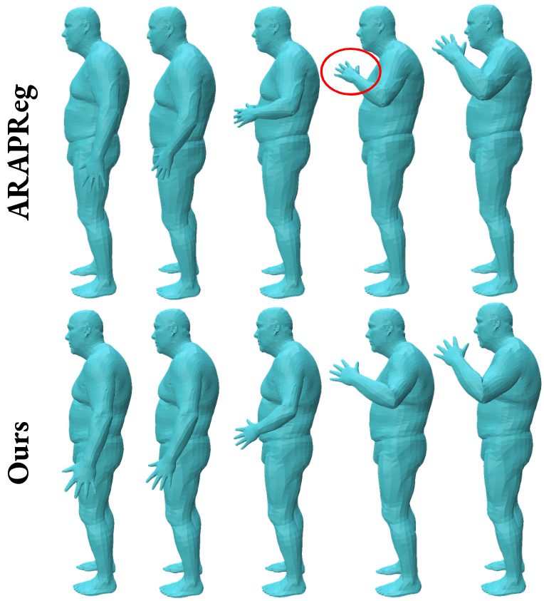
Figure 10: Qualitative comparison of latent interpolation. Our method shows more realistic interpolation trajectories, with limited distortion of the hand even with large non-linear deformations.

Partial deformations

Then we give another comparison of partial shape interpolation in Fig. 11.

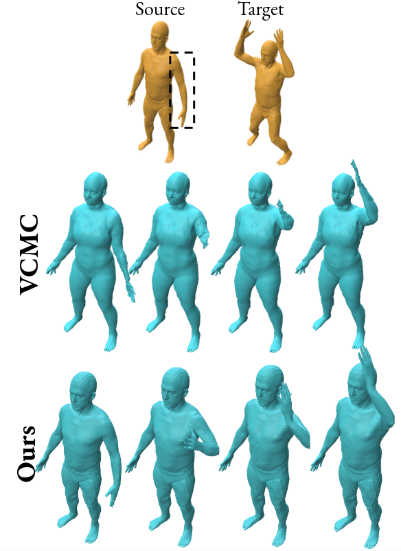
Figure 11: Qualitative comparison of partial latent interpolation. We computed a partial latent interpolation on an unseen identity between a source pose and a target pose displayed in yellow. The interpolated part is the left arm (dashed case). Previous comparable method VCMC fails to reconstruct the identity and exhibit important distortions of the selected part during the interpolation.

Applications: Shape statistics

As mentioned in the main paper, PaNDaS can be used to build statistical models of non-rigid deformations, such as the mean of shape collections. We demonstrate the robustness of our method by showing in Fig. 12 the generalizability of our trained model. The estimated mean from similar poses using PaNDaS is consistent across different identities.

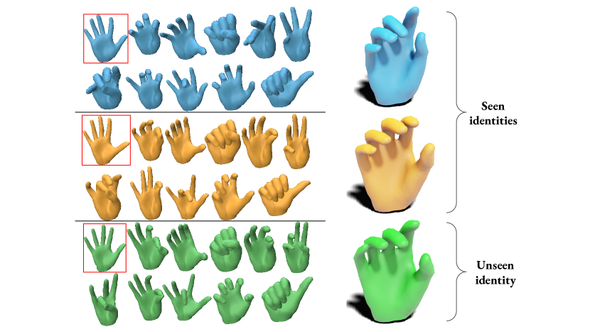
Figure 12: Robustness of the mean shape estimation. We perform mean shape estimation from a collection of 11 poses of hands. We predict the feature field associated with each pose and compute the Euclidean mean. The mean feature field is then used to compute the mean pose. In this figure, each color corresponds to a different identity (framed in red on the left). In particular, we highlight the robustness of our method across several hand identities, seen and unseen during training.

Applications: Partial Pose transfer

We give examples of partial pose/expression transfer in Fig. 13 and Fig. 14.

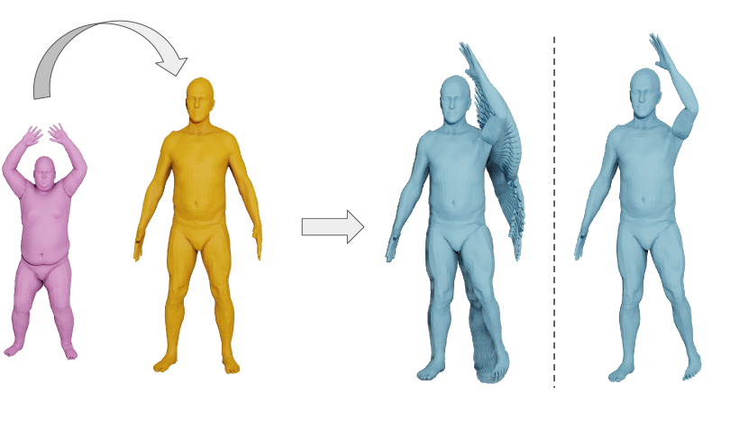
Figure 13: Example of partial pose transfer. In this example, the pose of the red mesh is transferred to the yellow mesh to produce a partial interpolation on the left side (in blue).

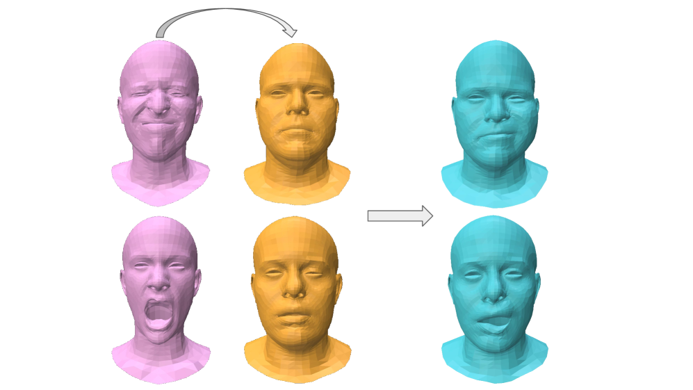
Figure 14: Example of partial expression transfer. In this example, the expression of the face in red is transferred to the yellow face restricted on the left side.

Appendix E Animations

We attached to the supplementary material, several videos showing animations (on the left side of the videos) computed with partial deformations extracted from combinations of different input poses (on the right side of the videos). PaNDaS can generate complex, controllable motions from a limited number of input poses.

References

- Aigerman et al. [2022] Noam Aigerman, Kunal Gupta, Vladimir G. Kim, Siddhartha Chaudhuri, Jun Saito, and Thibault Groueix. Neural jacobian fields: learning intrinsic mappings of arbitrary meshes. ACM Trans. Graph., 41(4), 2022.
- Alexa et al. [2000] Marc Alexa, Daniel Cohen-Or, and David Levin. As-rigid-as-possible shape interpolation. In Proceedings of the 27th Annual Conference on Computer Graphics and Interactive Techniques, page 157–164, USA, 2000. ACM Press/Addison-Wesley Publishing Co.
- Attaiki and Ovsjanikov [2022] Souhaib Attaiki and Maks Ovsjanikov. Ncp: Neural correspondence prior for effective unsupervised shape matching. Advances in Neural Information Processing Systems, 35:28842–28857, 2022.
- Bauer et al. [2011] Martin Bauer, Philipp Harms, and Peter W. Michor. Sobolev metrics on shape space of surfaces, 2011.
- Bauer et al. [2020] Martin Bauer, Nicolas Charon, Philipp Harms, and Hsi-Wei Hsieh. A numerical framework for elastic surface matching, comparison, and interpolation. International Journal of Computer Vision, 129:2425 – 2444, 2020.
- Beg et al. [2005] Mirza Faisal Beg, Michael Miller, Alain Trouvé, and Laurent Younes. Computing large deformation metric mappings via geodesic flows of diffeomorphisms. International Journal of Computer Vision, 61:139–157, 2005.
- Bogo et al. [2017] Federica Bogo, Javier Romero, Gerard Pons-Moll, and Michael J. Black. Dynamic FAUST: Registering human bodies in motion. In IEEE Conf. on Computer Vision and Pattern Recognition (CVPR), 2017.
- Botsch et al. [2006] Mario Botsch, Mark Pauly, Markus Gross, and Leif Kobbelt. Primo: coupled prisms for intuitive surface modeling. In Proceedings of the Fourth Eurographics Symposium on Geometry Processing, page 11–20, Goslar, DEU, 2006. Eurographics Association.
- Bouritsas et al. [2019] Giorgos Bouritsas, Sergiy Bokhnyak, Stylianos Ploumpis, Michael Bronstein, and Stefanos Zafeiriou. Neural 3d morphable models: Spiral convolutional networks for 3d shape representation learning and generation. In The IEEE International Conference on Computer Vision (ICCV), 2019.
- Cao et al. [2024] D. Cao, M. Eisenberger, N. El Amrani, D. Cremers, and F. Bernard. Spectral meets spatial: Harmonising 3d shape matching and interpolation. In 2024 IEEE/CVF Conference on Computer Vision and Pattern Recognition (CVPR), pages 3658–3668, Los Alamitos, CA, USA, 2024. IEEE Computer Society.
- Cosmo et al. [2020] Luca Cosmo, Antonio Norelli, Oshri Halimi, Ron Kimmel, and Emanuele Rodolà. Limp: Learning latent shape representations with metric preservation priors. In Computer Vision – ECCV 2020: 16th European Conference, Glasgow, UK, August 23–28, 2020, Proceedings, Part III, page 19–35, Berlin, Heidelberg, 2020. Springer-Verlag.
- Eisenberger et al. [2021] Marvin Eisenberger, David Novotny, Gael Kerchenbaum, Patrick Labatut, Natalia Neverova, Daniel Cremers, and Andrea Vedaldi. Neuromorph: Unsupervised shape interpolation and correspondence in one go. In Proceedings of the IEEE/CVF Conference on Computer Vision and Pattern Recognition, pages 7473–7483, 2021.
- Gong et al. [2019] Shunwang Gong, Lei Chen, Michael Bronstein, and Stefanos Zafeiriou. Spiralnet++: A fast and highly efficient mesh convolution operator. In Proceedings of the IEEE International Conference on Computer Vision Workshops, pages 0–0, 2019.
- Groueix et al. [2018] Thibault Groueix, Matthew Fisher, Vladimir G. Kim, Bryan Russell, and Mathieu Aubry. 3d-coded : 3d correspondences by deep deformation. In ECCV, 2018.
- Hahner et al. [2024] Sara Hahner, Souhaib Attaiki, Jochen Garcke, and Maks Ovsjanikov. Unsupervised representation learning for diverse deformable shape collections. In International Conference on 3D Vision 2024, 2024.
- Hartman et al. [2023a] Emmanuel Hartman, Emery Pierson, Martin Bauer, Nicolas Charon, and Mohamed Daoudi. BaRe-ESA: A riemannian framework for unregistered human body shapes. In Proceedings of the IEEE/CVF International Conference on Computer Vision (ICCV), pages 14181–14191, 2023a.
- Hartman et al. [2023b] Emmanuel Hartman, Yashil Sukurdeep, Eric Klassen, Nicolas Charon, and Martin Bauer. Elastic shape analysis of surfaces with second-order sobolev metrics: A comprehensive numerical framework. International Journal of Computer Vision, 2023b.
- Hartman et al. [2024] Emmanuel Hartman, Emery Pierson, Martin Bauer, Mohamed Daoudi, and Nicolas Charon. Basis restricted elastic shape analysis on the space of unregistered surfaces. International Journal of Computer Vision, 2024.
- Huang et al. [2021] Q. Huang, X. Huang, B. Sun, Z. Zhang, J. Jiang, and C. Bajaj. Arapreg: An as-rigid-as possible regularization loss for learning deformable shape generators. In 2021 IEEE/CVF International Conference on Computer Vision (ICCV), pages 5795–5805, Los Alamitos, CA, USA, 2021. IEEE Computer Society.
- Jermyn et al. [2012] Ian H Jermyn, Sebastian Kurtek, Eric Klassen, and Anuj Srivastava. Elastic shape matching of parameterized surfaces using square root normal fields. In European conference on computer vision, pages 804–817. Springer, 2012.
- Kilian et al. [2007] Martin Kilian, Niloy J Mitra, and Helmut Pottmann. Geometric modeling in shape space. In ACM SIGGRAPH 2007 papers, pages 64–es. 2007.
- Kingma and Ba [2015] Diederik Kingma and Jimmy Ba. Adam: A method for stochastic optimization. In International Conference on Learning Representations (ICLR), San Diega, CA, USA, 2015.
- Kurtek et al. [2011] Sebastian Kurtek, Eric Klassen, John C Gore, Zhaohua Ding, and Anuj Srivastava. Elastic geodesic paths in shape space of parameterized surfaces. IEEE transactions on pattern analysis and machine intelligence, 34(9):1717–1730, 2011.
- Laga et al. [2017] Hamid Laga, Qian Xie, Ian H Jermyn, and Anuj Srivastava. Numerical inversion of srnf maps for elastic shape analysis of genus-zero surfaces. IEEE transactions on pattern analysis and machine intelligence, 39(12):2451–2464, 2017.
- Lyu et al. [2023] Zhaoyang Lyu, Jinyi Wang, Yuwei An, Ya Zhang, Dahua Lin, and Bo Dai. Controllable mesh generation through sparse latent point diffusion models. In 2023 IEEE/CVF Conference on Computer Vision and Pattern Recognition (CVPR), pages 271–280, 2023.
- Magnet et al. [2022] Robin Magnet, Jing Ren, Olga Sorkine-Hornung, and Maks Ovsjanikov. Smooth non-rigid shape matching via effective dirichlet energy optimization. In 2022 International Conference on 3D Vision (3DV), pages 495–504, Los Alamitos, CA, USA, 2022. IEEE Computer Society.
- Muralikrishnan et al. [2024] Sanjeev Muralikrishnan, Niladri Shekhar Dutt, Siddhartha Chaudhuri, Noam Aigerman, Vladimir Kim, Matthew Fisher, and Niloy J. Mitra. Temporal residual jacobians for rig-free motion transfer, 2024.
- Qin et al. [2023] Dafei Qin, Jun Saito, Noam Aigerman, Groueix Thibault, and Taku Komura. Neural face rigging for animating and retargeting facial meshes in the wild. In SIGGRAPH 2023 Conference Papers, 2023.
- Ranjan et al. [2018] Anurag Ranjan, Timo Bolkart, Soubhik Sanyal, and Michael J. Black. Generating 3D faces using convolutional mesh autoencoders. In European Conference on Computer Vision (ECCV), pages 725–741, 2018.
- Romero et al. [2017] Javier Romero, Dimitrios Tzionas, and Michael J. Black. Embodied hands: Modeling and capturing hands and bodies together. ACM Transactions on Graphics, (Proc. SIGGRAPH Asia), 36(6), 2017.
- Schönemann [1966] Peter Schönemann. A generalized solution of the orthogonal procrustes problem. Psychometrika, 31(1):1–10, 1966.
- Sharp et al. [2022] Nicholas Sharp, Souhaib Attaiki, Keenan Crane, and Maks Ovsjanikov. Diffusionnet: Discretization agnostic learning on surfaces. ACM Trans. Graph., 01(1), 2022.
- Shi et al. [2023] Yujun Shi, Chuhui Xue, Jiachun Pan, Wenqing Zhang, Vincent YF Tan, and Song Bai. Dragdiffusion: Harnessing diffusion models for interactive point-based image editing. arXiv preprint arXiv:2306.14435, 2023.
- Sorkine and Alexa [2007] Olga Sorkine and Marc Alexa. As-rigid-as-possible surface modeling. In Proceedings of the Fifth Eurographics Symposium on Geometry Processing, page 109–116, Goslar, DEU, 2007. Eurographics Association.
- Tan et al. [2018] Qingyang Tan, Lin Gao, Yu-Kun Lai, and Shihong Xia. Variational autoencoders for deforming 3d mesh models. In 2018 IEEE/CVF Conference on Computer Vision and Pattern Recognition, pages 5841–5850, 2018.
- Tan et al. [2022] Qingyang Tan, Ling-Xiao Zhang, Jie Yang, Yu-Kun Lai, and Lin Gao. Variational autoencoders for localized mesh deformation component analysis. IEEE Transactions on Pattern Analysis and Machine Intelligence, 44(10):6297–6310, 2022.
- Xie et al. [2024] Tianhao Xie, Eugene Belilovsky, Sudhir Mudur, and Tiberiu Popa. Dragd3d: Realistic mesh editing with rigidity control driven by 2d diffusion priors, 2024.
- Xingang et al. [2023] Pan Xingang, Tewari Ayush, Leimkuhler Thomas, Li Lingjie, Meka Abhimitra, and Theobalt Christian. Drag your gan: Interactive point-based manipulation on the generative image manifold. In ACM SIGGRAPH 2023 Conference Proceedings, 2023.
- Yang et al. [2023] Haitao Yang, Bo Sun, Liyan Chen, Amy Pavel, and Qixing Huang. Geolatent: A geometric approach to latent space design for deformable shape generators. ACM Trans. Graph., 42(6), 2023.
- Yang et al. [2024] Haitao Yang, Xiangru Huang, Bo Sun, Chandrajit L. Bajaj, and Qixing Huang. Gencorres: Consistent shape matching via coupled implicit-explicit shape generative models. In The Twelfth International Conference on Learning Representations, 2024.
- Yoo et al. [2024] Seungwoo Yoo, Kunho Kim, Vladimir G. Kim, and Minhyuk Sung. As-Plausible-As-Possible: Plausibility-Aware Mesh Deformation Using 2D Diffusion Priors. In CVPR, 2024.
- Zhou et al. [2020] Yi Zhou, Chenglei Wu, Zimo Li, Chen Cao, Yuting Ye, Jason Saragih, Hao Li, and Yaser Sheikh. Fully convolutional mesh autoencoder using efficient spatially varying kernels. In Proceedings of the 34th International Conference on Neural Information Processing Systems, Red Hook, NY, USA, 2020. Curran Associates Inc.