Data dependent Moving Least Squares
Abstract
In this paper, we address a data dependent modification of the moving least squares (MLS) problem. We propose a novel approach by replacing the traditional weight functions with new functions that assign smaller weights to nodes that are close to discontinuities, while still assigning smaller weights to nodes that are far from the point of approximation. Through this adjustment, we are able to mitigate the undesirable Gibbs phenomenon that appears close to the discontinuities in the classical MLS approach, and reduce the smearing of discontinuities in the final approximation of the original data. The core of our method involves accurately identifying those nodes affected by the presence of discontinuities using smoothness indicators, a concept derived from the data-dependent WENO method. Our formulation results in a data-dependent weighted least squares problem where the weights depend on two factors: the distances between nodes and the point of approximation, and the smoothness of the data in a region of predetermined radius around the nodes. We explore the design of the new data-dependent approximant, analyze its properties including polynomial reproduction, accuracy, and smoothness, and study its impact on diffusion and the Gibbs phenomenon. Numerical experiments are conducted to validate the theoretical findings, and we conclude with some insights and potential directions for future research.
keywords:
WENO , high accuracy approximation , improved adaption to discontinuities , MLS , 41A05 , 41A10 , 65D05 , 65M06 , 65N061 Introduction and review
The Moving Least Squares (MLS) method, that was originally proposed by Shepard in [23] and further developed by Lancaster and Salkauskas in [15], is a powerful mathematical tool for generating smooth surfaces from scattered data points and for mess free aproximation of data. The MLS method has been widely applied in various fields such as data approximation [17], image processing [16], and geometric modelling [27], among others.
In the classical MLS approach, the goal is to approximate a function given a set of scattered data points . The more general form of the MLS approximation at a point is obtained by minimizing a weighted least squares error:
| (1) |
where is a weight function that decreases with the distance between and , are basis functions, and are the coefficients to be determined. The weight function is designed so that points closer to have a larger influence on the approximation.
Despite its effectiveness in smooth regions, the classical MLS method tends to produce oscillations near jump discontinuities. This limitation arises because the method assumes a smooth underlying function, which is not valid in the presence of discontinuities. Various strategies have been proposed to address this issue, including modifications to the weight function and the introduction of data-dependent techniques [25, 10].
In this work, we propose a data-dependent modification to the classical MLS method, inspired by the Weighted Essentially Non-Oscillatory (WENO) algorithm [19, 14]. Our purpose is to handle discontinuities more effectively including a data-dependent modification in the minimization problem (1). Our approach can be interpreted as an artificial adjustment of the distances of points near discontinuities, thereby reducing oscillations and improving the accuracy of the approximation. In the next subsection, we briefly introduce the WENO method, that will serve as inspiration for the data-dependent modification that we propose afterwards.
1.1 The Weighted Essentially Non-Oscillatory (WENO) method
The Weighted Essentially Non-Oscillatory (WENO) method was developed to solve hyperbolic partial differential equations with discontinuous solutions [14, 19]. The WENO algorithm builds upon the Essentially Non-Oscillatory (ENO) scheme [22], aiming to achieve high-order accuracy in smooth regions while avoiding spurious oscillations near discontinuities in the solution of conservation laws.
The key idea of the WENO method is to construct a weighted combination of several candidate stencils. For a given point, the WENO scheme selects the smoothest stencil by assigning weights that diminish the influence of stencils crossing discontinuities. The smoothness indicators are used to measure the smoothness of the function within each stencil, and the data-dependent weights are computed based on these indicators.
Consider a function that we want to approximate at the point . The WENO reconstruction for the function at is given by:
| (2) |
where is the number of stencils, are the polynomial approximations from each stencil, and are the data-dependent weights. The weights are computed as:
| (3) |
with
| (4) |
where are the linear weights, are the smoothness indicators, is a small positive number to avoid division by zero, and is a parameter typically set to 2 in order to obtain optimal accuracy at smooth zones. The smoothness indicators were designed in [14] using a measure of the smoothness of the underlying data inspired in the total variation:
| (5) |
where is the grid spacing. Given the nature of the problem we aim to solve, we will define the smoothness indicators differently. This approach is more suitable considering the scattered distribution of data points we are assuming. In the next subsection we explain the particular setting of our problem, including the description of the data and its distribution over the considered domain.
1.2 Our setting
We consider an open set, , that contains distinct nodes, and , that is the corresponding set of function values, where is unknown. Throughout this paper, we assume that the nodes are quasi-equally spaced (or equally spaced), and we define the fill distance (see, e.g. [11, 27, 28]) as:
| (6) |
we also choose a non-negative and compactly supported radial function , and define where is the Euclidean norm in (but any other norm can be used).
Let us consider a point . We particularize the moving least squares problem described in equation ((1)), to the polynomial approximation of the values . This involves calculating a polynomial of degree less than or equal to that closely approximates the given values at the points , and that satisfies:
| (7) |
Then, it is evaluated at , obtaining the approximation
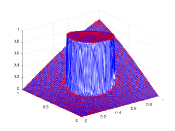
We can replace the condition that the function is compactly supported with the requirement that it decreases rapidly as . In this case, interpolation is achieved if , [17]. There are many formulations for this problem in approximation theory (see e.g., [6, 7, 8, 11, 17]) and in statistics, where it is known as local polynomial regression (see e.g., [11, 20]). The core idea of the method is to give more importance to the nodes near the point where we want to approximate. This method is effective because it can reproduce polynomials of degree , which implies an accuracy order of , and its smoothness depends on the chosen function . However, if the data points have a strong gradient or come from a discontinuous function, some oscillations may appear near the discontinuity, as shown in Figure 1.
| Original | MLS | MLS |
|---|---|---|
|
|
|
In particular, this paper considers a curve defined as the zero level set of a continuous level-set function . This function delineates two distinct sets within the domain
| (8) |
The unknown function is defined as:
| (9) |
with and . In this paper, we replace the functions in (7), which determine the importance of each node, with a new function that assigns a greater weight if the nodes are far from the discontinuity. In this way, we avoid the undesired effects produced by these nodes, and the Gibbs phenomenon is mitigated. The key to the method is to correctly detect the infected nodes using smoothness indicators, a concept defined in the context of data-dependent methods such as WENO (see e.g., [24]). Therefore, our problem is a weighted least squares problem where the weights depend on different aspects, in this case, two: the distances between the nodes and the point to approximate, and the distance between the isolated discontinuity and the nodes. We could change these particular requirements to others, such as the density of points or the monotonicity of the data.
We divide the paper into four sections: We start by defining the ingredients to design the new data dependent approximator in Section 2. The next section is devoted to analyzing the properties of the method, such as the reproduction of polynomials, the accuracy, and the smoothness presented by the new operator. Additionally, a study about the diffusion and the Gibbs phenomenon is shown. Some numerical experiments are performed to check the theoretical results in Section 4. Finally, some conclusions and future work are indicated in the last section.
2 The data dependent MLS method
The MLS problem that we consider, Eq. (7), can be reformulated from an algebraic point of view (see e.g., [20, 18]). We explain it for , but it is similar for any . Thus, we consider , , the set of polynomials of degree less than or equal to
and a basis of defined by:
Let , we define the matrices , as:
If we write
with
then the problem defined in Eq. (7) can be expressed as:
| (10) |
whose solution is
So we get that
| (11) |
Remark 1
Note that if is compactly supported then some points such that could exist. In these cases, we denote as:
and construct the same problem replacing by . In the rest of the paper, we consider that , for all
In the solution of the MLS problem exposed before, we can see that the relevance of the matrix is checked, such that weights are assigned depending on the distance of the nodes with respect to the point where we want to obtain the approximation. If the data points present an isolated discontinuity described by an unknown curve , then not only the distance but also the position of the nodes with respect to this curve are relevant. Therefore, in order to take into account these two variables, we construct a different problem by replacing the weight function with a data-dependent one. Thus, we define
| (12) |
where and are two parameters. We use to avoid zero values in the denominator. The purpose of is to reach the maximum order of accuracy of the approximation at smooth zones (see [24]). Typically, we use . Finally, the values with are the smoothness indicators, i.e., the values which mark if one node is close to the discontinuity or not. In our case, we determine a ball centered in the node with a fixed radius denoted by
and impose the following conditions (see e.g. [3]):
-
P1
The order of a smoothness indicator that is free of discontinuities is , i.e.
-
P2
When the stencil crosses a discontinuity, then
In this paper, we define the smoothness indicators in the following way: First we solve the linear least squares problem:
| (13) |
and compute the smoothness indicators as:
| (14) |
With this definition, satisfies P1 and P2. Now, with the new functions , defined in (12), we can pose the weighted least squares problem and find its solution. To do so, we define
and get the new data dependent approximation DD-MLS as in Eq. (11):
| (15) |
If we write , then we have that is a radial function since
with compact support, which assigns small weights (or zero) when the point is far from , but also, from the fact that or depending on whether is close to or far from a discontinuity, the function assigns larger weights to non-infected points and smaller (close to zero) weights to infected ones (meaning by infected, nodes that are at a distance smaller than from the discontinuity). In other words, we can interpret this data-dependent modification as a a change in the distance to the nodes that are close to discontinuities. All the nodes close to the discontinuity are considered to be far from any point and their importance is neglected in the final approximation. With these ingredients, in the next section we prove some properties of the new approximation technique.
3 Properties of the new method
In this section, we prove some properties of the approximation technique described in the previous section. In particular, we focus on the smoothness, the reproduction of polynomials, the order of accuracy and the elimination of Gibbs phenomenon:
-
•
Let us start with the smoothness: it is clear by Eq. (15) that if has maximum rank, i.e. , then the matrix is non-singular, since all the entries of the matrix are positive by Remark 1. Therefore, the smoothness of the new approximator depends only on the function since . We summarize this property in the next Theorem (Th. 3.1)
Theorem 3.1
Let , , be a function with , then the new approximation defined in Eq. (15) is .
In the literature there are many functions which are used in radial basis approximation. We summarize some of them in Table 1 (see e.g. [11, 28]).
RBF Gaussian G Inverse MultiQuadratic IMQ Matérn M0 Matérn M2 Matérn M4 Wendland W0 Wendland W2 Wendland W4 Table 1: Examples of RBFs. -
•
The second property is the reproduction of polynomials. As is non-singular, the system has a unique solution. If the data are the discretization of a polynomial of degree less than or equal to , then the solution of the problem Eq. (7) with instead of is the same. Therefore, the interpolator reproduces . The next result collects this property.
Theorem 3.2
Let be an open set, , a set of distinct nodes and a corresponding set of function values with . Then the data dependent MLS approximation defined in Eq. (15) satisfies
A direct consequence of the last Theorem, Th. 3.2, is the order of accuracy. If we consider the fill distance , Eq. (6), then we can assure that if the function is continuous, the order of accuracy is . Thus, we can enunciate the following corollary.
Corollary 3.3
Let . If , are quasi-uniformly distributed with fill distance , the weight function is compactly supported with support size , then the new approximation defined in Eq. (15) fulfills
where is a constant independent of .
-
•
Finally, we analyze the approximation when some points far enough from the discontinuities are used mixed with infected points. In this way, we will suppose that we have at least data points not marked as infected.
Theorem 3.4
Let be an open set, a set of distinct nodes with fill distance , and the corresponding set of function values with defined in Eq. (9). Let and let
as the set of points used to calculate the approximation at , with . We assume there exist at least points belonging to , denoted by , such that their smoothness indicators are of order , all located within . We further assume that the interpolation operator in defined using these points is well-defined, and that a constant independent of bounds its norm. Then the data dependent MLS approximation satisfies:
with .
Proof.Let be a point in . We divide the set
with and . Let us define to be polynomial interpolating at the points and, as all the non-infected data are at one side of the discontinuity, then
The MLS solution is defined by
Since and
| (16) |
it follows that
From (16), we know that the right-hand side of the inequality is bounded, then there exists a constant such that
| (17) |
independent of . By (16), if , and this implies that
then
with . Therefore,
Since, the interpolation operator is well-defined with respect to the points and its inverse is bounded by a constant independent of then
Therefore,
In our case, we only have to take in order to get the maximum order of accuracy.
Remark 2
Diffusion and oscillations in the MLS method. When applying the linear MLS method to discontinuous data with a radial weight function of support , the resulting approximation exhibits significant diffusion and oscillations within a region of width near the discontinuity curve .
The following theorem demonstrates that the diffusion region is significantly reduced when using the data dependent MLS method, and, additionally, oscillations are eliminated. We use the above definitions of , and and of defined in Eq. (9). We consider a weight function of support size , , and such that . We further assume that is a smooth curve. We adopt below the assumptions in Theorem 3.4 and the notation within its proof. Let denote the domain consisting of all points within a distance from , and let denote its complement.
Theorem 3.5
Assume the data points are within and let . Then the data dependent MLS approximation of degree with of support size satisfies
Proof.Define the support of data points respect to as . For any point the smoothness indicator is . Additionally, within a circular segment of width there are points for which the smoothness indicator is as .
Recalling that is the fill distance of the points , it follows that there exist at least points points for which the smoothness indicator is as . For these points, the interpolation operator, defined using them, is well-defined and its norm is bounded by a constant independent of . Then, by Theorem 3.4, using , the data dependent MLS approximation satisfies:
Corollary 3.6
Reduced diffusion region and reduced oscillations
The linear MLS provides full approximation order for points at a distance from . By applying Theorem 3.5 we observe that the data dependent MLS extends this full approximation order to a larger region, specifically to points at a distance from .
The oscillations observed near in the linear MLS approximation arise because it incorporates data from both sides of and applies both positive and negative weights. This occurs for points at a distance from . As argued in Theorem 3.5, for points within the range , the data dependent MLS approximation uses data only from one side of . Since the weights in the approximation sum to 1, and are applied exclusively to data from one side of , no oscillations will occur within this range.
4 Numerical experiments
In this section, we check numerically the theoretical properties shown in Section 3: order of accuracy, reproduction of polynomials, reduction of Gibbs oscillations, and reduction of the smearing around discontinuities.
The algorithm that we use is similar to the one designed in Chapter 19 of [11], we only introduce a detection of discontinuity points by calculating the smoothness indicator of each data point, i.e., we solve the problems in Eq. (13) and evaluate Eq. (14). For this problem, we fix the following parameter as in [9]:
where is the floor function, which returns the greatest integer less than or equal to . This part is not very expensive computationally because it only involves solving a simple linear least squares problem. Therefore, the algorithms for the linear and data-dependent cases are very similar in terms of computational cost.
We will use the acronyms or to call the linear and data dependent moving least squares methods, where represents the weight function, chosen from Table 1, and is the maximum degree of the polynomial used. We have selected the Wendland , functions and gaussian function to perform the experiments. We apply these functions in the following way, with . In our experiments, we take:
Also, in the Gaussian case, another condition is imposed: we only consider the values such that . We divide our experiments in three subsections: we examine the order of accuracy in smooth zones for the values . After that, we analyze the behaviour of the approximations close to the discontinuities, and, finally, we study intensively the smearing of discontinuities when (Shepard’s method, [23]) and .
4.1 Order of accuracy
We start by analyzing the order of accuracy using the well-known Franke’s function, defined as
| (18) |
using as nodes two types of sets: a regular grid defined by , and a collection of Halton’s scattered data points, as described in [13]. We denote the fill distance by , and the associated errors by , where is a regular grid in , and represents the set of evaluation points at which the function is approximated with points. Finally, we define the maximum discrete norms and their respective convergence rates as follows:
When , we can see in Tables 2 and 3 that the order of accuracy reached is greater than 3. In fact, when the data points are placed on a regular grid, the order of accuracy is close to 4 in both linear and data-dependent cases. These results are shown in Table 2. We can see that the error is slightly small when the linear version of the MLS is employed. This effect can be reduced if we choose a value of the parameter in (12) smaller, but then some oscillations can appear in the final approximation. When , Tables 4 and 5, the order of accuracy is 2 when using a regular grid, as it can be observed in Table 4, and also when using pseudo-random points, Table 5. Again, the error is slightly greater in the data-dependent case. Finally, when the order of accuracy with regular data points is larger than the one expected, as it is shown in Table 6, but smaller when Halton’s data points are used, as shown in Table 7. It is clear that the results when the data dependent MLS method is used are very close to the linear ones, and that it works correctly for smooth functions and, therefore, in the smooth zones.
| MLS | DD-MLS | MLS | DD-MLS | ||||||||
|---|---|---|---|---|---|---|---|---|---|---|---|
| 2.9459e-02 | 6.2989e-02 | 4.5011e-03 | 1.2700e-02 | ||||||||
| 3.4607e-03 | 3.1049 | 9.5840e-03 | 2.7299 | 4.0810e-04 | 3.4805 | 1.5139e-03 | 3.0837 | ||||
| 2.5977e-04 | 3.7728 | 9.5542e-04 | 3.3594 | 2.7858e-05 | 3.9111 | 1.3019e-04 | 3.5747 | ||||
| 1.7035e-05 | 3.9115 | 5.1915e-05 | 4.1814 | 1.7626e-06 | 3.9629 | 5.6006e-06 | 4.5168 | ||||
| MLS | DD-MLS | MLS | DD-MLS | ||||||||
| 2.1519e-02 | 4.7609e-02 | 3.0906e-03 | 9.0872e-03 | ||||||||
| 2.2812e-03 | 3.2538 | 6.5667e-03 | 2.8721 | 2.6332e-04 | 3.5707 | 1.0050e-03 | 3.1924 | ||||
| 1.6727e-04 | 3.8069 | 6.3657e-04 | 3.4002 | 1.7560e-05 | 3.9451 | 8.5276e-05 | 3.5941 | ||||
| 1.0846e-05 | 3.9276 | 3.3648e-05 | 4.2210 | 1.1183e-06 | 3.9536 | 3.6034e-06 | 4.5425 | ||||
| MLS | DD-MLS | MLS | DD-MLS | ||||||||
| 1.1701e-02 | 3.0202e-02 | 1.5423e-03 | 4.9530e-03 | ||||||||
| 1.0906e-03 | 3.4403 | 3.4672e-03 | 3.1383 | 1.2017e-04 | 3.7001 | 4.8617e-04 | 3.3654 | ||||
| 7.8215e-05 | 3.8392 | 3.1008e-04 | 3.5176 | 8.0812e-06 | 3.9330 | 3.9902e-05 | 3.6427 | ||||
| 5.2402e-06 | 3.8807 | 1.5806e-05 | 4.2732 | 5.6088e-07 | 3.8300 | 1.6869e-06 | 4.5417 | ||||
| MLS | DD-MLS | MLS | DD-MLS | ||||||||
|---|---|---|---|---|---|---|---|---|---|---|---|
| 3.0411e-02 | 5.3557e-02 | 4.5092e-03 | 1.2182e-02 | ||||||||
| 3.9097e-03 | 3.3987 | 9.7501e-03 | 2.8224 | 5.1659e-04 | 3.5898 | 1.5725e-03 | 3.3920 | ||||
| 4.9130e-04 | 3.4450 | 1.0768e-03 | 3.6595 | 5.4169e-05 | 3.7456 | 1.4011e-04 | 4.0161 | ||||
| 6.2966e-05 | 3.4057 | 1.3020e-04 | 3.5022 | 6.7078e-06 | 3.4627 | 9.2877e-06 | 4.4986 | ||||
| MLS | DD-MLS | MLS | DD-MLS | ||||||||
| 2.3547e-02 | 4.3721e-02 | 3.3430e-03 | 8.6294e-03 | ||||||||
| 2.7803e-03 | 3.5398 | 6.7029e-03 | 3.1071 | 3.8656e-04 | 3.5744 | 1.0595e-03 | 3.4750 | ||||
| 4.1415e-04 | 3.1625 | 7.9889e-04 | 3.5329 | 4.3740e-05 | 3.6192 | 9.6392e-05 | 3.9815 | ||||
| 6.4247e-05 | 3.0891 | 1.0343e-04 | 3.3890 | 5.8562e-06 | 3.3333 | 7.2394e-06 | 4.2916 | ||||
| MLS | DD-MLS | MLS | DD-MLS | ||||||||
| 1.8162e-02 | 3.1263e-02 | 2.2047e-03 | 4.8132e-03 | ||||||||
| 2.2788e-03 | 3.4391 | 4.5951e-03 | 3.1769 | 2.7608e-04 | 3.4424 | 5.6946e-04 | 3.5364 | ||||
| 3.8683e-04 | 2.9455 | 5.4298e-04 | 3.5472 | 3.3817e-05 | 3.4875 | 5.4933e-05 | 3.8842 | ||||
| 5.6293e-05 | 3.1951 | 8.6890e-05 | 3.0376 | 4.8183e-06 | 3.2301 | 5.2895e-06 | 3.8797 | ||||
| MLS | DD-MLS | MLS | DD-MLS | ||||||||
|---|---|---|---|---|---|---|---|---|---|---|---|
| 1.1379e-01 | 1.9511e-01 | 2.9208e-02 | 4.1874e-02 | ||||||||
| 3.1759e-02 | 1.8502 | 5.4100e-02 | 1.8597 | 8.2129e-03 | 1.8395 | 9.5939e-03 | 2.1364 | ||||
| 8.5522e-03 | 1.9115 | 1.1477e-02 | 2.2591 | 2.1242e-03 | 1.9703 | 2.1849e-03 | 2.1557 | ||||
| 2.2003e-03 | 1.9490 | 2.3391e-03 | 2.2835 | 5.3588e-04 | 1.9773 | 5.3824e-04 | 2.0114 | ||||
| MLS | DD-MLS | MLS | DD-MLS | ||||||||
| 8.9718e-02 | 1.5742e-01 | 2.3062e-02 | 3.2179e-02 | ||||||||
| 2.4477e-02 | 1.8833 | 4.3323e-02 | 1.8707 | 6.3336e-03 | 1.8737 | 7.1698e-03 | 2.1769 | ||||
| 6.5848e-03 | 1.9130 | 8.3406e-03 | 2.4005 | 1.6265e-03 | 1.9807 | 1.6580e-03 | 2.1334 | ||||
| 1.6836e-03 | 1.9580 | 1.7678e-03 | 2.2273 | 4.0947e-04 | 1.9802 | 4.1084e-04 | 2.0030 | ||||
| MLS | DD-MLS | MLS | DD-MLS | ||||||||
| 5.5298e-02 | 9.7249e-02 | 1.4210e-02 | 1.8864e-02 | ||||||||
| 1.4845e-02 | 1.9067 | 2.5712e-02 | 1.9288 | 3.7812e-03 | 1.9195 | 4.0917e-03 | 2.2158 | ||||
| 3.9269e-03 | 1.9375 | 4.6121e-03 | 2.5035 | 9.6173e-04 | 1.9947 | 9.7048e-04 | 2.0965 | ||||
| 9.9534e-04 | 1.9705 | 1.0290e-03 | 2.1536 | 2.4153e-04 | 1.9837 | 2.4203e-04 | 1.9938 | ||||
| MLS | DD-MLS | MLS | DD-MLS | ||||||||
|---|---|---|---|---|---|---|---|---|---|---|---|
| 1.0485e-01 | 1.9775e-01 | 2.8246e-02 | 4.2458e-02 | ||||||||
| 3.4265e-02 | 1.8530 | 4.9345e-02 | 2.3000 | 8.2717e-03 | 2.0348 | 9.6733e-03 | 2.4507 | ||||
| 9.7104e-03 | 2.0943 | 1.1974e-02 | 2.3520 | 2.1446e-03 | 2.2420 | 2.2221e-03 | 2.4431 | ||||
| 2.4667e-03 | 2.2716 | 2.4842e-03 | 2.6073 | 5.4304e-04 | 2.2769 | 5.4552e-04 | 2.3282 | ||||
| MLS | DD-MLS | MLS | DD-MLS | ||||||||
| 8.3978e-02 | 1.5293e-01 | 2.2556e-02 | 3.2350e-02 | ||||||||
| 2.8296e-02 | 1.8024 | 3.7951e-02 | 2.3092 | 6.4277e-03 | 2.0800 | 7.2640e-03 | 2.4748 | ||||
| 8.1573e-03 | 2.0659 | 8.9301e-03 | 2.4031 | 1.6564e-03 | 2.2522 | 1.6989e-03 | 2.4132 | ||||
| 2.1030e-03 | 2.2471 | 2.0241e-03 | 2.4606 | 4.1929e-04 | 2.2774 | 4.1958e-04 | 2.3183 | ||||
| MLS | DD-MLS | MLS | DD-MLS | ||||||||
| 5.7777e-02 | 8.1826e-02 | 1.4432e-02 | 1.8700e-02 | ||||||||
| 2.1624e-02 | 1.6284 | 2.5200e-02 | 1.9514 | 3.9649e-03 | 2.1406 | 4.2732e-03 | 2.4458 | ||||
| 6.1526e-03 | 2.0876 | 6.3276e-03 | 2.2953 | 1.0226e-03 | 2.2508 | 1.0340e-03 | 2.3568 | ||||
| 1.5647e-03 | 2.2698 | 1.5688e-03 | 2.3118 | 2.5971e-04 | 2.2719 | 2.5859e-04 | 2.2975 | ||||
| MLS | DD-MLS | MLS | DD-MLS | ||||||||
|---|---|---|---|---|---|---|---|---|---|---|---|
| 1.1379e-01 | 2.1215e-01 | 2.9355e-02 | 7.9470e-02 | ||||||||
| 3.1754e-02 | 1.8504 | 9.1316e-02 | 1.2222 | 8.3385e-03 | 1.8247 | 3.0115e-02 | 1.4069 | ||||
| 8.5514e-03 | 1.9115 | 3.1215e-02 | 1.5640 | 2.1290e-03 | 1.9891 | 8.2379e-03 | 1.8887 | ||||
| 2.2009e-03 | 1.9485 | 5.6983e-03 | 2.4417 | 5.3596e-04 | 1.9803 | 1.0663e-03 | 2.9352 | ||||
| MLS | DD-MLS | MLS | DD-MLS | ||||||||
| 8.9721e-02 | 1.8258e-01 | 2.3203e-02 | 6.5426e-02 | ||||||||
| 2.4474e-02 | 1.8835 | 7.5082e-02 | 1.2884 | 6.3935e-03 | 1.8688 | 2.4098e-02 | 1.4481 | ||||
| 6.5832e-03 | 1.9132 | 2.4913e-02 | 1.6074 | 1.6274e-03 | 1.9936 | 6.4179e-03 | 1.9277 | ||||
| 1.6845e-03 | 1.9569 | 4.4363e-03 | 2.4773 | 4.0959e-04 | 1.9806 | 8.1827e-04 | 2.9570 | ||||
| MLS | DD-MLS | MLS | DD-MLS | ||||||||
| 5.5301e-02 | 1.3307e-01 | 1.4256e-02 | 4.4167e-02 | ||||||||
| 1.4844e-02 | 1.9068 | 5.0079e-02 | 1.4169 | 3.7889e-03 | 1.9212 | 1.5365e-02 | 1.5308 | ||||
| 3.9248e-03 | 1.9382 | 1.5705e-02 | 1.6896 | 9.6178e-04 | 1.9976 | 3.8797e-03 | 2.0053 | ||||
| 9.9655e-04 | 1.9679 | 2.6784e-03 | 2.5393 | 2.4169e-04 | 1.9828 | 4.8548e-04 | 2.9838 | ||||
| MLS | DD-MLS | MLS | DD-MLS | ||||||||
|---|---|---|---|---|---|---|---|---|---|---|---|
| 1.0586e-01 | 2.4268e-01 | 2.8270e-02 | 8.4870e-02 | ||||||||
| 3.4724e-02 | 1.8469 | 9.8871e-02 | 1.4877 | 9.3858e-03 | 1.8269 | 3.1069e-02 | 1.6650 | ||||
| 1.3981e-02 | 1.5109 | 3.3478e-02 | 1.7986 | 2.8053e-03 | 2.0059 | 9.1451e-03 | 2.0313 | ||||
| 6.1264e-03 | 1.3678 | 9.2646e-03 | 2.1296 | 1.0559e-03 | 1.6198 | 1.6218e-03 | 2.8673 | ||||
| MLS | DD-MLS | MLS | DD-MLS | ||||||||
| 8.2583e-02 | 2.0157e-01 | 2.2883e-02 | 7.0341e-02 | ||||||||
| 3.3019e-02 | 1.5189 | 8.3508e-02 | 1.4600 | 7.8197e-03 | 1.7791 | 2.5145e-02 | 1.7044 | ||||
| 1.5863e-02 | 1.2176 | 3.1235e-02 | 1.6334 | 2.6272e-03 | 1.8116 | 7.4538e-03 | 2.0196 | ||||
| 6.7009e-03 | 1.4285 | 9.0153e-03 | 2.0599 | 1.1405e-03 | 1.3833 | 1.5213e-03 | 2.6344 | ||||
| MLS | DD-MLS | MLS | DD-MLS | ||||||||
| 7.5331e-02 | 1.4497e-01 | 1.6087e-02 | 4.8153e-02 | ||||||||
| 3.2711e-02 | 1.3821 | 6.3294e-02 | 1.3731 | 6.3405e-03 | 1.5427 | 1.6858e-02 | 1.7389 | ||||
| 1.8551e-02 | 0.9421 | 2.8400e-02 | 1.3311 | 2.7718e-03 | 1.3743 | 5.3489e-03 | 1.9067 | ||||
| 8.8940e-03 | 1.2187 | 1.0852e-02 | 1.5948 | 1.4143e-03 | 1.1155 | 1.5756e-03 | 2.0262 | ||||
4.2 Avoiding oscillations
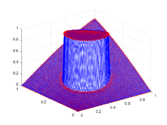
In this subsection, we approximate some functions with discontinuities as we have defined in Eq. 9. We start by approximating the function, on , defined in [2]:
| (19) |
using grid data points, Figure 2.a) using the linear method, and Figure 2.b), using W2. When a polynomial of degree is used, we can see that some oscillations appear close to the discontinuities, Figure 2.a), in the linear case. This phenomenon is not avoided even if we refine the mesh. We can observe that these non-desired oscillations disappear when the data-dependent method is employed, Figure 2.b). This result is very similar when the data points are pseudorandom, Figures 2.c) and 2.d). If the approximator is , Figures 2.e) and 2.f), then the result is similar, but in the DD-MLS we can observe that some smearing of the discontinuities appears.

|
|
|
|
| a) MLS | b) DD-MLS |
|
|
| c) MLS | d) DD-MLS |
|
|
| e) MLS | f) DD-MLS |
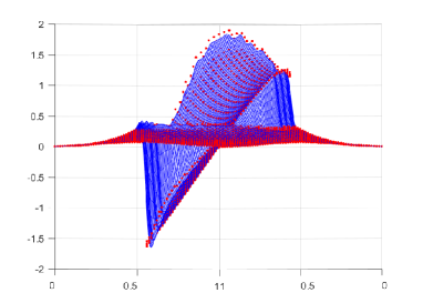
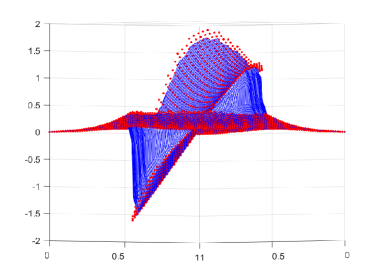
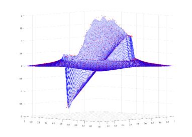
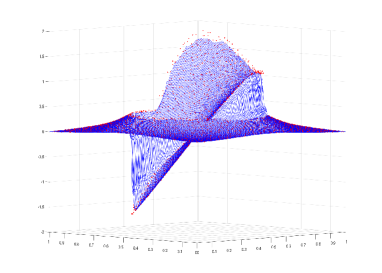
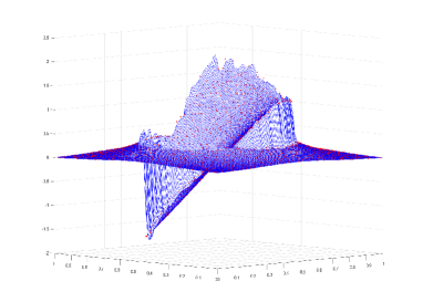
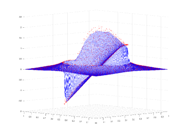
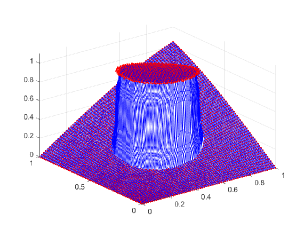
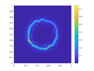
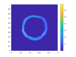
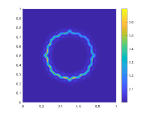
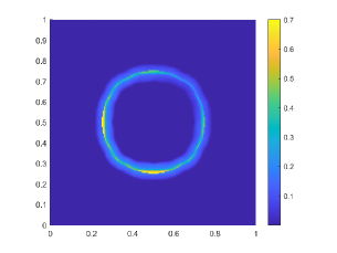
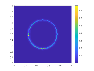
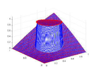
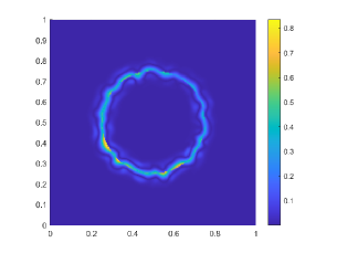
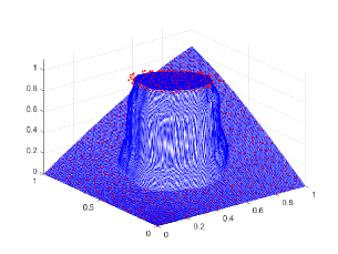
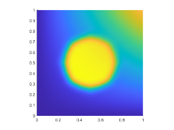
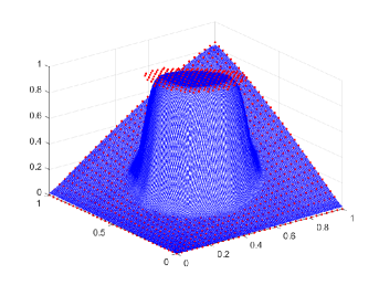
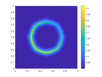
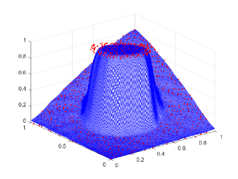
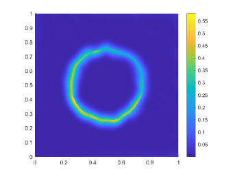
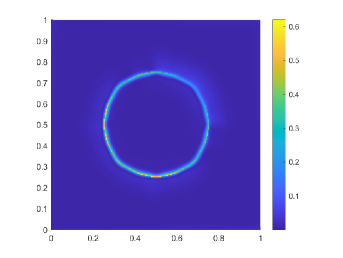
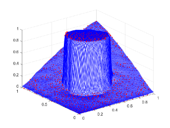
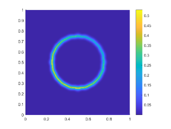
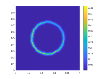
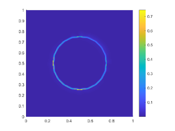
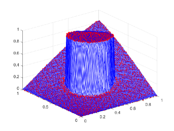
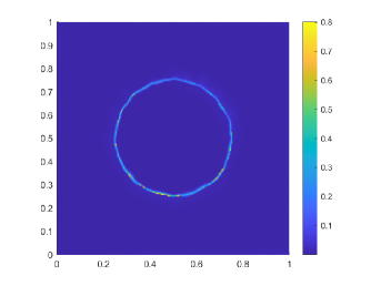
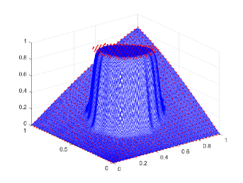
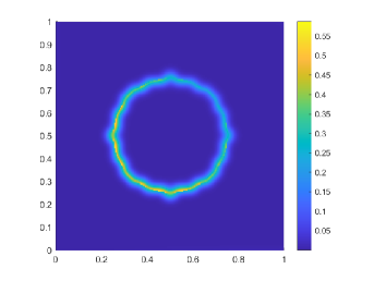
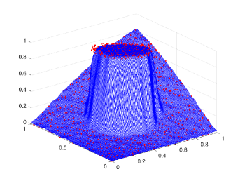
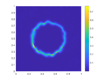
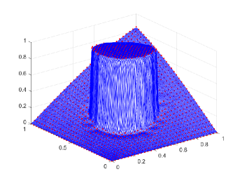
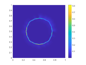
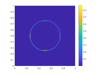
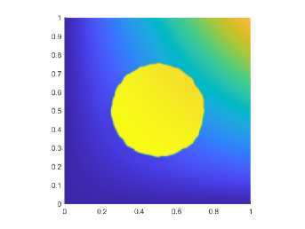
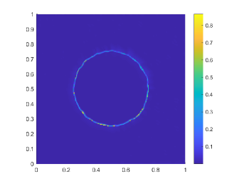
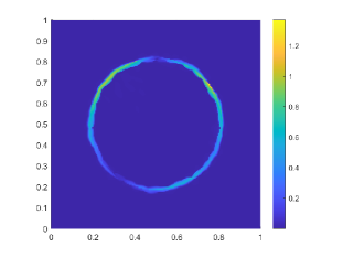
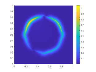
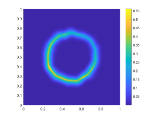
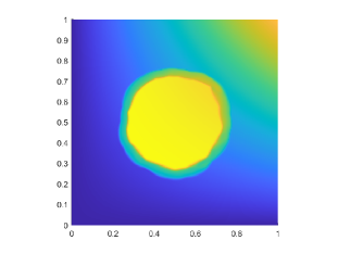
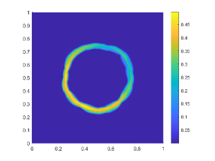
In order to analyze the behaviour when the discontinuity is more pronounced, we perform the example designed in [1] with the following function
| (20) |
In this experiment, Figures 3 and 4, we show the result using and data points, and the error between the original function and the approximated one. We can observe that the non-desired oscillations disappear for W2 and G cases.
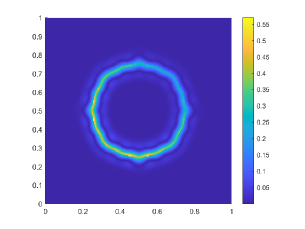


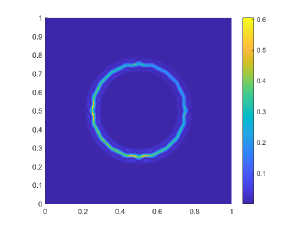


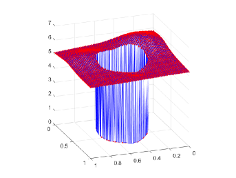
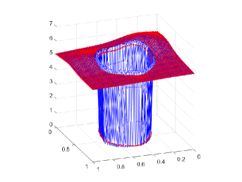
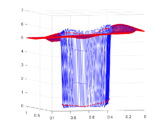
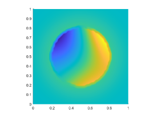
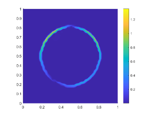
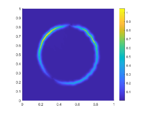
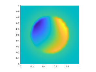
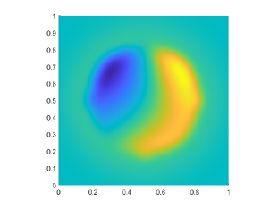
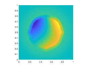
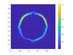
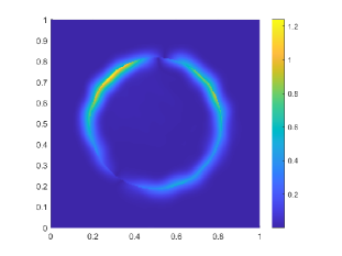
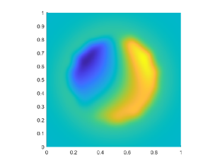
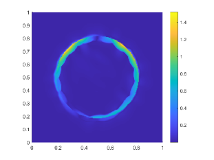
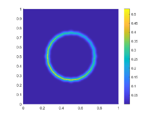
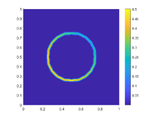
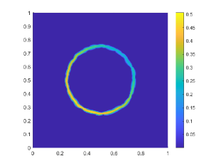
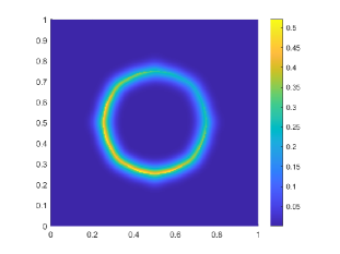
4.3 Reduction of the smearing zone across the discontinuity
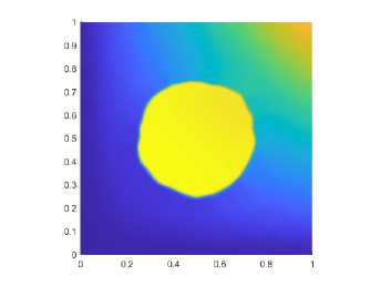
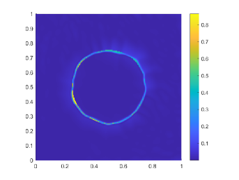
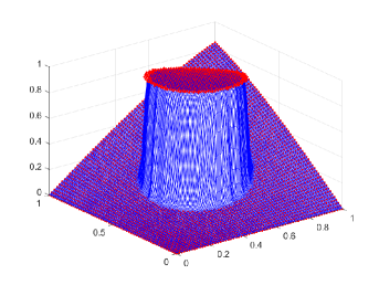
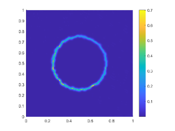
In this section we study the results obtained when we employ the set of polynomials of degree , general Shepard’s method (see [11]), or . In these cases, the non-desired oscillations do not occur, but some diffusion effects appear when the linear MLS algorithms are used. We compare these linear algorithms with the data-dependent ones using the same function, , Eq. (20). We perform experiments with , Figures 5 and 7 and , Figures 6 and 8, using W2 and G functions, and for gridded and Halton’s data points. In all the results, we can observe that the discontinuity is perfectly delineated in both the case of regular meshes and with Halton’s points. Particularly striking is the result obtained for the function G, Figures 7 and 8, where the band of diffusion around the discontinuity is reduced considerably.
| MLS | |||
| 2D-plot | Approximation | Error | |
|
|
|
|

|
|
|
|
| DD-MLS | |||

|

|
|
|

|
|

|
|
| MLS | |||
| 2D-plot | Approximation | Error | |

|

|
|
|

|

|
|
|
| DD-MLS | |||

|
|
|
|

|
|
|
|
| MLS | |||
| 2D-plot | Approximation | Error | |

|
|
|
|

|
|
|
|
| DD-MLS | |||

|
|
|
|
|

|
|
|
| MLS | ||
| 2D-plot | Approximation | Error |

|
|

|

|

|
|
| DD-MLS | ||

|
|
|
|

|
|
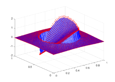
Finally, some examples with are shown in Figures 9 and 10. Again, the diffusion effects decrease using DD-MLS.
| MLS | DD-MLS | ||
|---|---|---|---|

|

|
|
|
|
|

|
|
|
|
|
|
|
|

|
|
| MLS | DD-MLS | ||
|---|---|---|---|
|

|

|
|

|

|

|
|
|

|

|

|
|

|
|
|
5 Conclusions and Future work
In this study, we have introduced a novel approach to the moving least squares (MLS) problem (7) by replacing the traditional weight functions with new functions that assign greater weight to nodes farther from discontinuities, while still assigning smaller weights to nodes far from the point of approximation. This adjustment effectively mitigates the Gibbs phenomenon and reduces the smearing of discontinuities in the final approximation of the original data.
Our method uses smoothness indicators to accurately identify infected nodes, i.e. those affected by the presence of discontinuities, in a way inspired by the WENO method. This results in a data-dependent weighted least squares problem where the weights are influenced by both the distances between nodes and the point of approximation, and the distances between isolated discontinuities and the nodes. We think that these criteria could be adapted to other requirements, such as point density or monotonicity, but we leave these ideas for future explorations.
Through the design and analysis of the new data dependent approximation, we have demonstrated its properties, including polynomial reproduction, accuracy, smoothness or neglecting of the Gibbs oscillations close to the discontinuities. Our numerical experiments validate the theoretical findings, showing the effectiveness of the proposed method.
References
- [1] S. Amat, D. Levin, J. Ruiz, D. F. Yáñez (2024): “Non-linear WENO B-spline based approximation method”, Numer. Algorithms.
- [2] A. Amir, D. Levin, (2021): “Reconstructing piecewise smooth bivariate functions from scattered data”, Jaen J. Approx., 12, 155–173.
- [3] F. Aràndiga, A. M. Belda, P. Mulet, (2010): “Point-Value WENO Multiresolution Applications to Stable Image Compression”, J. Sci. Comput., 43(2), 158–182.
- [4] F. Aràndiga and R. Donat, (2000) “Nonlinear multiscale decompositions: The approach of Ami Harten”, Numer. Algorithms, 23:175–216, 2000.
- [5] A. Baeza, R. Bürger, P. Mulet, D. Zorío, (2019): “Central WENO schemes through a global average weight”, J. Sci. Comput. 78, 499–530.
- [6] G. Backus and F. Gilbert, (1967): “Numerical applications of a formalism for geophysical inverse problems”, Geophys. J.R. Astr. Soc. 13, 247–276.
- [7] G. Backus and F. Gilbert, (1968): “The resolving power of gross Earth data”, Geophys. J.R. Astr. Soc. 16, 169–205.
- [8] L. Bos and K. Salkauskas, (1989): “Moving least-squares are Backus-Gilbert optimal”, J. Approx. Theory 59, 267–275.
- [9] A. De Rossi, R. Cavoretto, E. Perracchione, S. Lancellotti, (2022): “Software Implementation of the Partition of Unity Method ”, Dolomites Research Notes on Approximation 15(2), 35–46.
- [10] M. K. Esfahani, S. De Marchi, and F. Marchetti, (2023). “Moving Least Squares Approximation using Variably Scaled Discontinuous Weight Function,” arXiv preprint arXiv:2302.02707.
- [11] G. E. Fasshauer: Meshfree Approximation Methods with Matlab, World Scientific Publishing, Singapore, 2007.
- [12] D. Gottlieb, C-W. Shu, (1997): On the Gibbs phenomenon and its resolution. SIAM Rev., 39 (4), 644-668.
- [13] J.H. Halton (1960): “On the efficiency of certain quasi-random sequences of points in evaluating multi-dimensional integrals”, Numer. Math., 2:84–90.
- [14] G. Jiang and C.-W. Shu, (1996): “Efficient Implementation of Weighted ENO Schemes”, J. Comput. Phys., 126(1), 202-228.
- [15] P. Lancaster and K. Salkauskas, (1981). “Surfaces generated by moving least squares methods,” Mathematics of Computation, vol. 37, no. 155, pp. 141–158, JSTOR.
- [16] Y. J. Lee, G. Wolberg, and S. Y. Shin, (1997). “Image morphing using moving least squares,” Proceedings of the 24th annual conference on Computer graphics and interactive techniques, ACM Press/Addison-Wesley Publishing Co., pp. 21–28.
- [17] D. Levin, (1998): “The approximation power of Moving least-squares”, Math. Comput. 67, 224.
- [18] S. López-Ureña, D. F. Yáñez, (2024): “Subdivision schemes based on weighted local polynomial regression. A new technique for the convergence analysis.”, J. Sci. Comput., 100 (10).
- [19] X.-D. Liu and S. Osher and T. Chan, (1994): “Weighted Essentially Non-oscillatory Schemes”, J. Comput. Phys., 115, 200-212.
- [20] C. Loader: Local Regression and likelihook, Springer, New York, 1999.
- [21] A. Harten, (1996): “Multiresolution representation of data: a general framework”, SIAM J. Numer. Anal., 33(3) 1205–1256.
- [22] A. Harten, B. Engquist, S. Osher, and S. R. Chakravarthy, (1987). “Uniformly high order accurate essentially non-oscillatory schemes, III,” Journal of Computational Physics, vol. 71, no. 2, pp. 231–303, Elsevier.
- [23] D. Shepard, (1968). “A two-dimensional interpolation function for irregularly-spaced data”, Proceedings of the 1968 23rd ACM national conference., 517-524.
- [24] C.-W. Shu, (1999): “High Order Weighted Essentially Nonoscillatory Schemes for Convection Dominated Problems”, SIAM Review, 51(1), 82–126.
- [25] W. Y. Tey, N. A. C. Sidik, Y. Asako, M. W. Muhieldeen, and O. Afshar, (2021). “Moving Least Squares Method and its Improvement: A Concise Review,” Journal of Applied and Computational Mechanics, vol. 7, no. 2, pp. 883–889, Shahid Chamran University of Ahvaz.
- [26] H. Wendland, (1995). “Piecewise polynomial, positive definite and compactly supported radial functions with minimal degree”, Adv. in Comput. Math., 4, 389–396.
- [27] H. Wendland, (2004). “Scattered Data Approximation”, Cambridge University Press.
- [28] H. Wendland, (2002). “Fast Evaluation of Radial Basis Functions: Methods based on partition of unity ”, Approximation Theory X: Wavelets, Splines and Applications, C. K. Chui, L. L. Schumaker, and J. Stöcker (eds.) Vanderbilt University Press.