We introduce a new method designed for Bayesian inference of the angular power spectrum of the Gravitational Wave Background (GWB) anisotropy. This scheme works with time-series data and can optionally incorporate the cross-correlations between the GWB anisotropy and other cosmological tracers, enhancing the significance of Bayesian inference. We employ the realistic LISA response and noise model to demonstrate the validity of this approach. The findings indicate that, without considering any cross-correlations, the 4-year LISA data is insufficient to achieve a significant detection of multipoles. However, if the anisotropies in the GWB are strongly correlated with the Cosmic Microwave Background (CMB), the 4-year data can provide unbiased estimates of the quadrupole moment (). This reconstruction process is generic and not restricted to any specific detector, offering a new framework for extracting anisotropies in the GWB data from various current and future gravitational wave observatories.
Introduction —
Our ability to detect gravitational waves (GWs) will undoubtedly reach an unprecedented level in the next decade, with detection ranges spanning from nanohertz to several hundred hertz and significantly enhanced precision.
This substantial advancement is likely to help us fully decipher a new background signal in the Universe — the gravitational wave background (GWB), whose preliminary clues have been revealed by recent Pulsar Timing Array experiments Agazie et al. (2023); Xu et al. (2023); Antoniadis et al. (2023); Reardon et al. (2023).
This diffused GW signal, resulting from superpositions of numerous unresolved sources, can be classified into two categories: the astrophysical gravitational wave background (AGWB) and the cosmological gravitational wave background (CGWB). The former results from superpositions of unresolved galactic and extra-galactic sources, mostly related to the dynamics of compact objects Ferrari et al. (1999a, b); Schneider et al. (2001); Farmer and Phinney (2003); Regimbau (2011); Zhu et al. (2011). The latter, originating from early Universe processes, is closely related to new physics, such as inflation, reheating/preheating, primordial black holes, topological defects, or cosmological first-order phase transitions Vachaspati and Vilenkin (1985); Kosowsky et al. (1992); Guzzetti et al. (2016); Caprini and Figueroa (2018); Aggarwal et al. (2021).
Similar to the CMB and other cosmological probes, the GWB also carries anisotropies, which can originate from either source distributions or propagation processes. Anisotropies arising from sources include those generated by inhomogeneous distributions of compact objects Alba and Maldacena (2016), in the case of the AGWB, or those resulting from large scale perturbations introduced by domain walls in the early universe Liu et al. (2021), as in the CGWB. On the other hand, the propagation process may lead to anisotropies due to various gravitational effects, analogous to the CMB photons Contaldi (2017). Considerable efforts have been made in recent years to model the angular power spectrum of the GWB anisotropy Geller et al. (2018); Bartolo et al. (2019, 2020); Valbusa Dall’Armi et al. (2021); Li et al. (2022); Schulze et al. (2023); Cui et al. (2023); Wang et al. (2023); Li et al. (2023); Valbusa Dall’Armi et al. (2023); Bethke et al. (2013); Cusin et al. (2017, 2018); Jenkins et al. (2019); Cusin et al. (2019); Bertacca et al. (2020); Bellomo et al. (2022); Sato-Polito and Kamionkowski (2023); Pol et al. (2022); Yu and Wang (2024) and to assess its detectability in the operating and proposed GW observations Alonso et al. (2020a, b); Ricciardone et al. (2021); Capurri et al. (2022); Jenkins et al. (2018); Zhao and Wang (2024); Capurri et al. (2023). These investigations have primarily focused on signal-to-noise ratio (SNR) estimations or sky map reconstructions Renzini and Contaldi (2018, 2019); Banagiri et al. (2021); Bartolo et al. (2022); Chung and Yunes (2023); Tsukada et al. (2023); Gair et al. (2014); Li et al. (2024). However, to facilitate a comparison with physical models, a Bayesian framework for extracting angular spectra directly from time-series data is necessary. Moreover, as predicted by many theoretical studies Ricciardone et al. (2021); Ding and Tian (2024); Schulze et al. (2023); Yang et al. (2023), regardless of their astrophysical or cosmological origins, the anisotropies in the GWB generally exhibit significant cross-correlations with other existing cosmological tracers, such as the CMB, the CMB lensing, or large-scale structures. The detection sensitivity to the anisotropies would undoubtedly benefit from these potential cross-correlations, as suggested by Capurri et al. (2022); Alonso et al. (2020a); Ricciardone et al. (2021), through estimating the enhanced SNR. Nevertheless, a consistent methodology for integrating these cross-correlations into the data-analysis framework, facilitating the extraction of the angular power spectrum of the GWB anisotropy, has not been established.
In this letter, we focus on a novel data analysis scheme designed to extract anisotropies in the form of the angular power spectrum directly from time-series data of GW detectors. This framework optionally accounts for the potential cross-correlations between the anisotropic GWB and other cosmological tracers. We demonstrate the validity of this approach by applying it to LISA Amaro-Seoane et al. (2017); Arun et al. (2022) mock data and discuss its broader applications for future GW observations.
Anisotropic GWB intensity and time-series data —
Assuming the GWs to be Gaussian, stationary and unpolarized, the metric perturbation in Fourier space is characterized by its quadratic expectation values as
(1)
where labels the polarization states, is the direction of propagation in the sky and the matrix is related to the gravitational Stokes parameters , , and .
Under the unpolarized condition, , one has , where represents the GW intensity.
On the other hand, when considering the GWB, it’s a common practice to quantifying it through the fractional energy density , whose spectrum can be separated into a background part (monopole) and a linear fluctuation.
It can be proven Smith et al. (2019); Bartolo et al. (2022) the relationship between the anisotropic GW intensity and the fractional energy density, using the spherical harmonic coefficients, can be expressed by
(2)
and
(3)
where we have assumed that has encapsulated all the frequency dependencies, leaving s frequency-independent, which is exactly true when has a power-law spectrum. Our aim is to extract the power spectrum of , denoted as , from the time-series data.
The time-series data of a GW detector A, denoted as , is obtained by applying Fourier transforms to the signal over a specific time segment , at given time , resulting in
(4)
where and are the response function and noise for the detector . has a zero mean, and its ensemble average, evaluated at equal time and frequency (and is otherwise zero), can be estimated by
(5)
where is the noise power spectral density (PSD) for the detector pair , and are spherical harmonic coefficients of the response function for this detector pair, defined by
(6)
The covariance of , at the same time and frequency, can be written as
(7)
where we have dropped contributions from multipoles in the approximation, which are subdominant.
Likelihood with cross-correlations —
Our aim is to perform Bayesian estimations on the angular power spectrum of the GWB anisotropy using the time-series dataset . For this purpose, a practical likelihood function is necessary. When a set of is given, the likelihood for , which represents data for various detector’s combinations at a specific time and frequency, can be simply written as
(8)
However, for a given angular power spectrum , there are in principle an infinite number of realizations in terms of , preventing us from writing down a likelihood function that directly links the time-series data with the model predicted . Therefore, we must remain agnostic regarding specific realizations.
In addition, the GWB anisotropy may be correlated with other cosmological tracers. Assuming that the GWB is cross-correlated with a known cosmological tracer , it is acknowledged that maps of the GWB together with the tracer can be represented by multivariate Gaussian variables with the covariance specified by their auto angular spectra , and the cross spectrum . Consequently, the conditional probability for the GWB can be derived with the knowledge of , whose measured spherical harmonics coefficients are with negligible uncertainties compared to the GWB measurements. It can be proven that for a given condition characterized by the combination of , the conditional distribution of at a given frequency, denoted as , obeys
(9)
where we have defined the mean and the auto-correlation of this GWB anisotropy as
To finally derive the likelihood for the entire data set while remaining agonistic to the specific realization, we marginalize over all s and sum over contributions from all time and frequency bins by computing
Note that all quantities in eq. (13) depend on the time and frequencies, and for simplicity, we have used Latin letters, such as a and b, to compress the detector combinations, such as , into a single index. Additionally, we use Greek letters , , etc., to denote combinations of s. Following this convention, we have also defined , and for and (see eq. (2)) for . We also denote to be the covariance described in eq. (7) and to be a diagonal matrix expanded from by
(16)
Eqs eqs.13, 14 and 15 are the main results of this letter. It is also important to know that this likelihood is generic, being applicable to models that are not considering any cross-correlations. In such case, one has , and the mean and the covariance of harmonic coefficients are reduced to for and , producing a likelihood function of GW angular power spectrum without considering any cross-correlations, similarly as the results in van Haasteren and Levin (2013); Gair et al. (2014).
Bayesian inference of LISA mock data —
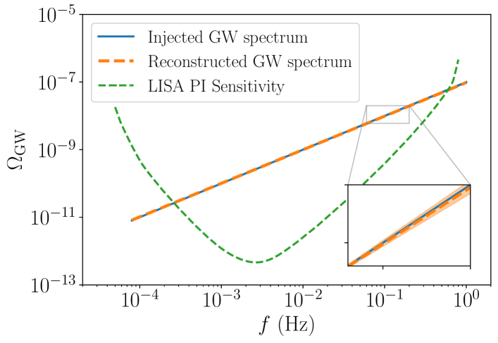
For demonstration purposes, we inject anisotropic GWB signals to LISA and attempt to estimate the injected anisotropic level. The injected signal has a power-law spectrum , where we have chosen , and , as depicted in the upper panel of Fig. 1. It is a relatively strong signal compared to the LISA sensitivity and the predicted spectrum of compact binaries Ferrari et al. (1999a, b); Schneider et al. (2001); Farmer and Phinney (2003); Regimbau (2011). Therefore, this mock signal can be considered as a GWB from new physics, which may arise from first order phase transitions or inflationary models (see Caprini et al. (2024); Bartolo et al. (2016) for comprehensive reviews) .
Figure 1: Upper Panel: Injected and reconstructed GWB spectrum. The uncertainty is represented by the nearly invisible shaded region;
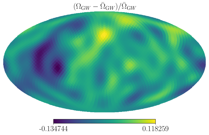
Lower Panel: The sky map of the injected GWB, with the angular power spectrum satisfying . Map pixels’ locations are following the HealPixGórski et al.(2005) convention with .
The anisotropies in the signal are generated based on a scale invariant angular spectrum of s, implying that . This is a typical prediction of many cosmological models at low s. Ricciardone et al. (2021); Schulze et al. (2023); Ding and Tian (2024). Our primary task is to estimate the from the mock data. To this end, we generate a time-series data set following the covariance given by eq. (5) in the frequency range with . This frequency spacing corresponds to an observation segment , generating different observation segments in a year, corresponding to a observation efficiency. Each segment has a different antenna pattern due to the satellite array’s varying orientations over a year. We compute the LISA response and the noise PSD using the public code schNell Alonso et al. (2020b), which estimates the LISA time-dependent response function based on spacecraft positions over time, as derived in Rubbo et al. (2004), while assuming a time-independent noise Smith et al. (2019).
Once the fiducial data is injected, we first attempt to recover the monopole data (see Fig. 1). This can be simply done by employing eq. (13) and setting to zero. The nearly invisible shaded region indicates that the uncertainties in the reconstructed monopole signals are negligible. The small uncertainties suggest that the contributions from the multipoles in the likelihood can be safely ignored when inferring the monopole spectrum. We therefore fix the reconstructed monopole parameters during the subsequent inferences of the angular power spectrum.
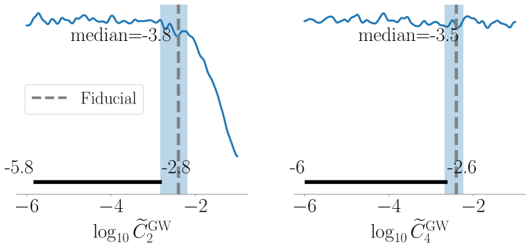
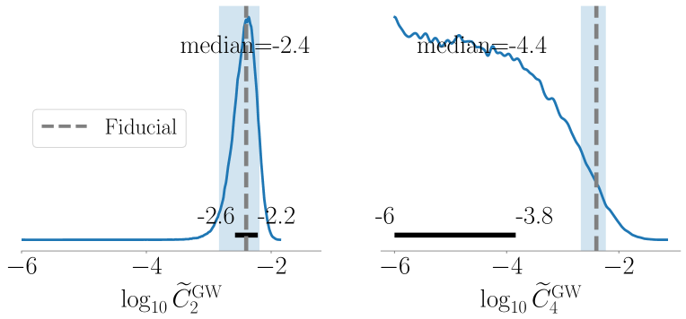
Figure 2: Upper Panel: Reconstructed multipoles and based on the LISA 4-year data. Fiducial . Lower Panel: Reconstructed multipoles based on the LISA 80-year data. Fiducial . The black bars on the bottom mark the region, and the shaded regions represent the cosmic variance.
We then employ the full likelihood in eq. (13) to estimate the magnitude of the lowest several multipoles. To avoid potential numerical instabilities in the matrix inverses, in our calculation, we compute the matrix inverse by expanding the term in eq. (14) to the 2nd order. The resulting posteriors are presented in Fig. 2. It is apparent that the LISA 4-year mission lacks sufficient sensitivity to recover the magnitude of multipoles in the GWB. This finding is consistent with other studies Alonso et al. (2020a); Capurri et al. (2022, 2023) based on the analysis of the SNR. Note that we only present the results for even multipoles, as the even parity of the LISA antenna patten results in a weak SNR in the odd multipoles. We also find that unrealistically extending the LISA mission to 80 years and increasing the anisotropic level to will result in a posterior for the quadrupole moment whose region is comparable to the cosmic variance Bernardo and Ng (2022), thereby suggesting the validity of our scheme.
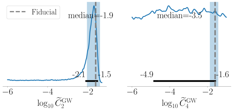
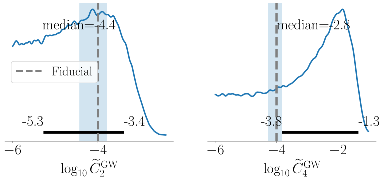
Figure 3: Reconstructed multipoles based on the LISA 4-year data, assuming a perfect cross-correlations between the GWB and the CMB. Upper Panel: The fiducial . Lower Panel: The fiducial . The black bars on the bottom mark the region, and the shaded regions represent the cosmic variance.
Depending on the sources, the anisotropies in the GWB generally show different levels of cross-correlations with diverse cosmological tracers. For the CGWB, current models suggest that it has a strong correlation with the CMB or the CMB lensing Ricciardone et al. (2021); Schulze et al. (2023); Ding and Tian (2024). To explore the most optimistic constraints on the LISA detectability based on known cross-correlations, we consider an ideal scenario in which the GWB is perfectly correlated with the CMB. Under this assumption, we inject a GWB fully correlated with the CMB by setting , subsequently employing this scheme to infer the magnitude of the lowest several multipoles in the GWB. Our findings indicate that the LISA 4-year data is able to provide unbiased estimations of quadrupole when , as suggested by the upper panel in Fig. 3, confirming the validity of our scheme. As the bottom panel in Fig. 3 implies, this reconstruction works until approximately .
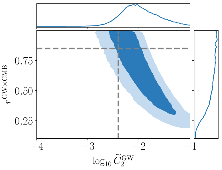
Figure 4: Contour and posterior plots of the quadrupole and relative cross-correlation. The fiducial and . The grey dashed lines denote the fiducial values. Shaded regions represent the and range.
We have also simulated a GWB map based on a smaller relative correlation with the CMB, specifically with . By employing the likelihood function given in eq. (13) and taking as a new parameter, we plot vs. contour in Fig. 4. The results indicate that, even under the condition of a weaker correlation, our scheme remains effective in inferring quadrupole : the fiducial value can still be recovered within a confident level.
Discussions — In this study, we introduce a novel scheme for performing Bayesian inference on time-series data associated with the stochastic gravitational wave background. Utilizing a new analytical likelihood function, this approach directly connects the time-series data to the angular power spectrum, with the capability to incorporate the cross-correlations between the GWB anisotropy and any cosmological tracers. As a crucial feature of the GWB anisotropy, these cross-correlations, predicted by various physical models, can significantly enhance the reconstruction capability of our framework.
We employ forecasted LISA response and noise to demonstrate the validity of this approach. Our findings indicate that, without considering any cross-correlations, the noise level in the 4-year LISA data prevents us from constructing reliable Bayesian inference on multipoles unless the LISA mission is unrealistically extended to 80 years. However, if the anisotropies in the GWB are strongly correlated with another cosmological tracer, such as the CMB, the 4-year LISA data can provide unbiased estimates of the quadrupole moment.
We emphasize that this scheme is designed generically for arrays of GW detectors. Our work, therefore, paves the way for detailed studies of the detectabilities of anisotropies in future ground-based and space-based GW observations, such as TianQin Luo et al. (2016), Taiji Hu and Wu (2017); Ruan et al. (2020), DECIGO Kawamura et al. (2011), BBO Hu and Wu (2017); Ruan et al. (2020), ET Maggiore et al. (2020), and their possible joint searches Torres-Orjuela et al. (2024); Torres-Orjuela (2024); Liang et al. (2024). The exploration of open questions, such as how various GWB source models are constrained from the GWB anisotropy, or how to differentiate between astrophysical and cosmological sources based on the anisotropies, might benefit from this new scheme. However, the focus of this letter is on the success of the method rather than the detectability for a specific detector or constraining GWB source models; we will therefore leave the detailed analysis on these topics for future studies.
Acknowledgments — Authors would like to thank Erik Floden, Vuk Mandic, Leo Tsukada and Gang Wang. R.D. is supported in part by the National Key R&D Program of China (No. 2021YFC2203100). C.T. is supported by the National Natural Science Foundation of China (Grants No. 12405048) and the Natural Science Foundation of Anhui Province (Grants No. 2308085QA34). The authors acknowledge the High-performance Computing Platform of Anhui University for providing computing resources.
Antoniadis et al. (2023)J. Antoniadis et al. (EPTA), “The second data release from the European Pulsar Timing Array III. Search for gravitational wave signals,” (2023), arXiv:2306.16214 [astro-ph.HE] .
Ferrari et al. (1999a)Valeria Ferrari, Sabino Matarrese, and Raffaella Schneider, “Stochastic background of gravitational waves generated by a cosmological population of young, rapidly rotating neutron stars,” Mon. Not. Roy. Astron. Soc. 303, 258 (1999a), arXiv:astro-ph/9806357 .
Zhu et al. (2011)Xing-Jiang Zhu, E. Howell, T. Regimbau, D. Blair, and Zong-Hong Zhu, “Stochastic Gravitational Wave Background from Coalescing Binary Black Holes,” Astrophys. J. 739, 86 (2011), arXiv:1104.3565 [gr-qc] .
Vachaspati and Vilenkin (1985)Tanmay Vachaspati and Alexander Vilenkin, “Gravitational Radiation from Cosmic Strings,” Phys. Rev. D 31, 3052 (1985).
Kosowsky et al. (1992)Arthur Kosowsky, Michael S. Turner, and Richard Watkins, “Gravitational waves from first order cosmological phase transitions,” Phys. Rev. Lett. 69, 2026–2029 (1992).
Geller et al. (2018)Michael Geller, Anson Hook, Raman Sundrum, and Yuhsin Tsai, “Primordial Anisotropies in the Gravitational Wave Background from Cosmological Phase Transitions,” Phys. Rev. Lett. 121, 201303 (2018), arXiv:1803.10780 [hep-ph] .
Bartolo et al. (2019)N. Bartolo, D. Bertacca, S. Matarrese, M. Peloso, A. Ricciardone, A. Riotto, and G. Tasinato, “Anisotropies and non-Gaussianity of the Cosmological Gravitational Wave Background,” Phys. Rev. D 100, 121501 (2019), arXiv:1908.00527 [astro-ph.CO] .
Bartolo et al. (2020)Nicola Bartolo, Daniele Bertacca, Sabino Matarrese, Marco Peloso, Angelo Ricciardone, Antonio Riotto, and Gianmassimo Tasinato, “Characterizing the cosmological gravitational wave background: Anisotropies and non-Gaussianity,” Phys. Rev. D 102, 023527 (2020), arXiv:1912.09433 [astro-ph.CO] .
Valbusa Dall’Armi et al. (2021)L. Valbusa Dall’Armi, A. Ricciardone, Nicola Bartolo, D. Bertacca, and S. Matarrese, “Imprint of relativistic particles on the anisotropies of the stochastic gravitational-wave background,” Phys. Rev. D 103, 023522 (2021), arXiv:2007.01215 [astro-ph.CO] .
Li et al. (2022)Yongping Li, Fa Peng Huang, Xiao Wang, and Xinmin Zhang, “Anisotropy of phase transition gravitational wave and its implication for primordial seeds of the Universe,” Phys. Rev. D 105, 083527 (2022), arXiv:2112.01409 [astro-ph.CO] .
Schulze et al. (2023)Florian Schulze, Lorenzo Valbusa Dall’Armi, Julien Lesgourgues, Angelo Ricciardone, Nicola Bartolo, Daniele Bertacca, Christian Fidler, and Sabino Matarrese, “GW_CLASS: Cosmological Gravitational Wave Background in the Cosmic Linear Anisotropy Solving System,” (2023), arXiv:2305.01602 [gr-qc] .
Cui et al. (2023)Yanou Cui, Soubhik Kumar, Raman Sundrum, and Yuhsin Tsai, “Unraveling Cosmological Anisotropies within Stochastic Gravitational Wave Backgrounds,” (2023), arXiv:2307.10360 [astro-ph.CO] .
Wang et al. (2023)Sai Wang, Zhi-Chao Zhao, Jun-Peng Li, and Qing-Hua Zhu, “Implications of Pulsar Timing Array Data for Scalar-Induced Gravitational Waves and Primordial Black Holes: Primordial Non-Gaussianity Considered,” (2023), arXiv:2307.00572 [astro-ph.CO] .
Li et al. (2023)Jun-Peng Li, Sai Wang, Zhi-Chao Zhao, and Kazunori Kohri, “Primordial Non-Gaussianity and Anisotropies in Scalar-Induced Gravitational Waves,” (2023), arXiv:2305.19950 [astro-ph.CO] .
Cusin et al. (2017)Giulia Cusin, Cyril Pitrou, and Jean-Philippe Uzan, “Anisotropy of the astrophysical gravitational wave background: Analytic expression of the angular power spectrum and correlation with cosmological observations,” Phys. Rev. D 96, 103019 (2017), arXiv:1704.06184 [astro-ph.CO] .
Jenkins et al. (2019)Alexander C. Jenkins, Richard O’Shaughnessy, Mairi Sakellariadou, and Daniel Wysocki, “Anisotropies in the astrophysical gravitational-wave background: The impact of black hole distributions,” Phys. Rev. Lett. 122, 111101 (2019), arXiv:1810.13435 [astro-ph.CO] .
Cusin et al. (2019)Giulia Cusin, Irina Dvorkin, Cyril Pitrou, and Jean-Philippe Uzan, “Properties of the stochastic astrophysical gravitational wave background: astrophysical sources dependencies,” Phys. Rev. D 100, 063004 (2019), arXiv:1904.07797 [astro-ph.CO] .
Bertacca et al. (2020)Daniele Bertacca, Angelo Ricciardone, Nicola Bellomo, Alexander C. Jenkins, Sabino Matarrese, Alvise Raccanelli, Tania Regimbau, and Mairi Sakellariadou, “Projection effects on the observed angular spectrum of the astrophysical stochastic gravitational wave background,” Phys. Rev. D 101, 103513 (2020), arXiv:1909.11627
[astro-ph.CO] .
Bellomo et al. (2022)Nicola Bellomo, Daniele Bertacca, Alexander C. Jenkins, Sabino Matarrese, Alvise Raccanelli, Tania Regimbau, Angelo Ricciardone, and Mairi Sakellariadou, “CLASS_GWB: robust modeling of the astrophysical gravitational wave background anisotropies,” JCAP 06, 030 (2022), arXiv:2110.15059 [gr-qc] .
Sato-Polito and Kamionkowski (2023)Gabriela Sato-Polito and Marc Kamionkowski, “Exploring the spectrum of stochastic gravitational-wave anisotropies with pulsar timing arrays,” (2023), arXiv:2305.05690 [astro-ph.CO] .
Pol et al. (2022)Nihan Pol, Stephen R. Taylor, and Joseph D. Romano, “Forecasting Pulsar Timing Array Sensitivity to Anisotropy in the Stochastic Gravitational Wave Background,” Astrophys. J. 940, 173 (2022), arXiv:2206.09936 [astro-ph.HE] .
Alonso et al. (2020a)David Alonso, Giulia Cusin, Pedro G. Ferreira, and Cyril Pitrou, “Detecting the anisotropic astrophysical gravitational wave background in the presence of shot noise through cross-correlations,” Phys. Rev. D 102, 023002 (2020a), arXiv:2002.02888 [astro-ph.CO] .
Alonso et al. (2020b)David Alonso, Carlo R. Contaldi, Giulia Cusin, Pedro G. Ferreira, and Arianna I. Renzini, “Noise angular power spectrum of gravitational wave background experiments,” Phys. Rev. D 101, 124048 (2020b), arXiv:2005.03001 [astro-ph.CO] .
Ricciardone et al. (2021)Angelo Ricciardone, Lorenzo Valbusa Dall’Armi, Nicola Bartolo, Daniele Bertacca, Michele Liguori, and Sabino Matarrese, “Cross-Correlating Astrophysical and Cosmological Gravitational Wave Backgrounds with the Cosmic Microwave Background,” Phys. Rev. Lett. 127, 271301 (2021), arXiv:2106.02591 [astro-ph.CO] .
Capurri et al. (2022)Giulia Capurri, Andrea Lapi, and Carlo Baccigalupi, “Detectability of the Cross-Correlation between CMB Lensing and Stochastic GW Background from Compact Object Mergers,” Universe 8, 160 (2022), arXiv:2111.04757 [astro-ph.CO] .
Jenkins et al. (2018)Alexander C. Jenkins, Mairi Sakellariadou, Tania Regimbau, and Eric Slezak, “Anisotropies in the astrophysical gravitational-wave background: Predictions for the detection of compact binaries by LIGO and Virgo,” Phys. Rev. D 98, 063501 (2018), arXiv:1806.01718 [astro-ph.CO] .
Capurri et al. (2023)Giulia Capurri, Andrea Lapi, Lumen Boco, and Carlo Baccigalupi, “Searching for Anisotropic Stochastic Gravitational-wave Backgrounds with Constellations of Space-based Interferometers,” Astrophys. J. 943, 72 (2023), arXiv:2212.06162 [gr-qc] .
Renzini and Contaldi (2019)Arianna Renzini and Carlo Contaldi, “Improved limits on a stochastic gravitational-wave background and its anisotropies from Advanced LIGO O1 and O2 runs,” Phys. Rev. D 100, 063527 (2019), arXiv:1907.10329 [gr-qc] .
Bartolo et al. (2022)Nicola Bartolo et al. (LISA Cosmology Working Group), “Probing anisotropies of the Stochastic Gravitational Wave Background with LISA,” JCAP 11, 009 (2022), arXiv:2201.08782 [astro-ph.CO] .
Chung and Yunes (2023)Adrian Ka-Wai Chung and Nicolas Yunes, “Untargeted Bayesian search of anisotropic gravitational-wave backgrounds through the analytical marginalization of the posterior,” Phys. Rev. D 108, 043032 (2023), arXiv:2305.06502 [gr-qc] .
Gair et al. (2014)Jonathan Gair, Joseph D. Romano, Stephen Taylor, and Chiara M. F. Mingarelli, “Mapping gravitational-wave backgrounds using methods from CMB analysis: Application to pulsar timing arrays,” Phys. Rev. D 90, 082001 (2014), arXiv:1406.4664 [gr-qc] .
Li et al. (2024)Zhi-Yuan Li, Zheng-Cheng Liang, En-Kun Li, Jian-dong Zhang, and Yi-Ming Hu, “Mapping Anisotropies in the Stochastic Gravitational-Wave Background with TianQin,” (2024), arXiv:2409.11245 [gr-qc] .
Ding and Tian (2024)Ran Ding and Chi Tian, “On the anisotropies of the cosmological gravitational-wave background from pulsar timing array observations,” JCAP 02, 016 (2024), arXiv:2309.01643 [astro-ph.CO] .
Yang et al. (2023)Kate Z. Yang, Jishnu Suresh, Giulia Cusin, Sharan Banagiri, Noelle Feist, Vuk Mandic, Claudia Scarlata, and Ioannis Michaloliakos, “Measurement of the cross-correlation angular power spectrum between the stochastic gravitational wave background and galaxy overdensity,” Phys. Rev. D 108, 043025 (2023), arXiv:2304.07621
[gr-qc] .
Amaro-Seoane et al. (2017)Pau Amaro-Seoane et al. (LISA), “Laser Interferometer Space Antenna,” (2017), arXiv:1702.00786 [astro-ph.IM] .
Smith et al. (2019)Tristan L. Smith, Tristan L. Smith, Robert R. Caldwell, and Robert Caldwell, “LISA for Cosmologists: Calculating the Signal-to-Noise Ratio for Stochastic and Deterministic Sources,” Phys. Rev. D 100, 104055 (2019), [Erratum: Phys.Rev.D 105, 029902 (2022)], arXiv:1908.00546 [astro-ph.CO] .
Caprini et al. (2024)Chiara Caprini, Ryusuke Jinno, Marek Lewicki, Eric Madge, Marco Merchand, Germano Nardini, Mauro Pieroni, Alberto Roper Pol, and Ville Vaskonen (LISA Cosmology Working Group), “Gravitational waves from first-order phase transitions in LISA: reconstruction pipeline and physics interpretation,” JCAP 10, 020 (2024), arXiv:2403.03723 [astro-ph.CO] .
Bartolo et al. (2016)Nicola Bartolo et al., “Science with the space-based interferometer LISA. IV: Probing inflation with gravitational waves,” JCAP 12, 026 (2016), arXiv:1610.06481 [astro-ph.CO] .
Górski et al. (2005)K. M. Górski, E. Hivon, A. J. Banday, B. D. Wandelt, F. K. Hansen, M. Reinecke, and M. Bartelman, “HEALPix - A Framework for high resolution discretization, and fast analysis of data distributed on the sphere,” Astrophys. J. 622, 759–771 (2005), arXiv:astro-ph/0409513 .
Bernardo and Ng (2022)Reginald Christian Bernardo and Kin-Wang Ng, “Pulsar and cosmic variances of pulsar timing-array correlation measurements of the stochastic gravitational wave background,” JCAP 11, 046 (2022), arXiv:2209.14834 [gr-qc] .
Hu and Wu (2017)Wen-Rui Hu and Yue-Liang Wu, “The Taiji Program in Space for gravitational wave physics and the nature of gravity,” Natl. Sci. Rev. 4, 685–686 (2017).
Torres-Orjuela et al. (2024)Alejandro Torres-Orjuela, Shun-Jia Huang, Zheng-Cheng Liang, Shuai Liu, Hai-Tian Wang, Chang-Qing Ye, Yi-Ming Hu, and Jianwei Mei, “Detection of astrophysical gravitational wave sources by TianQin and LISA,” Sci. China Phys. Mech. Astron. 67, 259511 (2024), arXiv:2307.16628 [gr-qc] .
Torres-Orjuela (2024)Alejandro Torres-Orjuela, “Joint gravitational wave detection by TianQin and LISA,” in 7th International Workshop on the TianQin Science Mission (2024) arXiv:2407.11293 [astro-ph.HE] .
Liang et al. (2024)Zheng-Cheng Liang, Zhi-Yuan Li, En-Kun Li, Jian-dong Zhang, and Yi-Ming Hu, “Unveiling a multi-component stochastic gravitational-wave background with the TianQin + LISA network,” (2024), arXiv:2409.00778 [gr-qc] .
Supplemental Material
I Conditional probability distribution considering cross-correlation angular power spectrum
A multidimensional complex Gaussian distribution for -dimensional variable is given by
(S1)
Suppose that the vector obeys joint gaussian distribution
(S6)
where is the non-symmetric cross-covariance matrix between and . Then the marginal distributions are
(S7)
and according to the definition, the conditional probability distributions are
(S8)
We now apply the results above to construct the likelihood function, incorporating the cross-correlations between the GWB and any known cosmological tracers. Assuming that the GWB and a set of cosmological tracers , characterized by spherical harmonic coefficients and respectively, are multivariate Gaussian random variables with zero mean and covariance . Following eq. (S6), their probability distribution is given by
(S15)
According to eq. (S8), the conditional distribution of for given obeys
We will show that eq. (S25) can be reformulated into a more concise expression, providing a clearer representation of the underlying physics. To see this, we employ Sherman-Morrison-Woodbury matrix inversion lemma, written as
(S29)
(S30)
where and are square and invertible matrices, though not necessarily of the same dimension. From which, adopting the matrix form, we obtain following relations:
(S31)
(S32)
(S33)
The exponential term in eq. (S25) can be rearranged to get
(S34)
Taking into account the determinants, eq. (S25) then becomes
(S35)
Finally, to combine two terms associated with , we define for and for , and redefine
(S36)
to match the matrix dimensions, arriving the likelihood function in eq. (13)