DSSRNN: Decomposition-Enhanced State-Space Recurrent Neural Network for Time-Series Analysis

Abstract.

Time series forecasting is a crucial yet challenging task in machine learning, requiring domain-specific knowledge due to its wide-ranging applications. While recent Transformer models have improved forecasting capabilities, they come with high computational costs. Linear-based models have shown better accuracy than Transformers but still fall short of ideal performance. To address these challenges, we introduce the Decomposition State-Space Recurrent Neural Network (DSSRNN), a novel framework designed for both long-term and short-term time series forecasting. DSSRNN uniquely combines decomposition analysis to capture seasonal and trend components with state-space models and physics-based equations. We evaluate DSSRNN’s performance on indoor air quality datasets, focusing on CO2 concentration prediction across various forecasting horizons. Results demonstrate that DSSRNN consistently outperforms state-of-the-art models, including transformer-based architectures, in terms of both Mean Squared Error (MSE) and Mean Absolute Error (MAE). For example, at the shortest horizon (T=96) in Office 1, DSSRNN achieved an MSE of 0.378 and an MAE of 0.401, significantly lower than competing models. Additionally, DSSRNN exhibits superior computational efficiency compared to more complex models. While not as lightweight as the DLinear model, DSSRNN achieves a balance between performance and efficiency, with only 0.11G MACs and 437MiB memory usage, and an inference time of 0.58ms for long-term forecasting. This work not only showcases DSSRNN’s success but also establishes a new benchmark for physics-informed machine learning in environmental forecasting and potentially other domains. To facilitate further research and application, we provide our datasets and code at https://github.com/ahmad-shirazi/DSSRNN.

1. Introduction

The prediction of complex time series data stands as a critical challenge in machine learning (ML), particularly where accuracy and computational efficiency intersect (Zhou et al., 2021; Lim et al., 2021; Zhou et al., 2022; Liu et al., 2022; Zhou et al., 2021; Zeng et al., 2023). Outlier events in time series, such as spikes or dips, can disrupt forecasting models, necessitating robust detection and handling methods to maintain accuracy (Blázquez-García et al., 2021). Time series are omnipresent in today’s data landscape, underpinning critical applications across various domains, from traffic flow estimation (Pamuła and Żochowska, 2023) and energy management (Chen et al., 2023) to financial investment (Barra et al., 2020; Sezer et al., 2020). In time series analysis, the challenge isn’t just long-term or short-term forecasting (Zeng et al., 2023) but also preparing datasets, often impeded by missing data(Che et al., 2018; Emmanuel et al., 2021). The integration of state-space models, founded on physics principles, with advanced ML techniques, presents a versatile solution that transcends domain boundaries (Kirchgässner et al., 2023; Fu et al., 2022; Xue et al., 2020). This synthesis transforms physics-based equations into computational algorithms, providing a robust framework capable of capturing the complex temporal dynamics across a range of real-world problems—from forecasting energy consumption in buildings to predicting building energy consumption (Somu et al., 2021; Pham et al., 2020; Olu-Ajayi et al., 2022; Zhang et al., 2021) and weather patterns(Bochenek and Ustrnul, 2022; Markovics and Mayer, 2022; Kashinath et al., 2021).

A significant portion of prior work in this area has focused on the use of transformers (Wen et al., 2022). However, transformers face several challenges in time series prediction. For long-term forecasting, their self-attention mechanism, which scales quadratically with sequence length, leads to high computational costs and memory usage. Capturing long-range dependencies effectively can be problematic, potentially diluting important signals over time. Transformers also suffer from the vanishing gradient problem and limitations of fixed context windows. In short-term prediction, transformers are prone to overfitting due to their high capacity, struggle with noise sensitivity, and may not generalize well with limited data. Despite shorter sequences, they remain computationally expensive compared to simpler models. Additionally, transformers require extensive hyperparameter tuning and are less interpretable than traditional models (Zeng et al., 2023). Our methodology addresses these limitations through the use of state-space models that capture the dynamics of complex systems (Friedland, 2012), essentially marrying the precision of physics with the adaptability of machine learning. This integrated approach enables prediction accuracy while optimizing computational resources.

Our research, though broadly applicable, specifically targets the domain of Indoor Air Quality (IAQ), with a particular focus on predicting carbon dioxide ($CO_{2}$) levels. This variable is of critical health relevance and presents significant predictive challenges due to its nonlinear behavior and sensitivity to numerous factors, including human occupancy, activity patterns, and ventilation systems (Taheri and Razban, 2021). The complexity of $CO_{2}$ dynamics makes it ideal for demonstrating our models’ efficacy in handling intricate dependencies and varying conditions.

We validate our work in a range of indoor environments, showing that our model surpasses existing benchmarks in accuracy and efficiency. Its success in forecasting using data with a range of characteristics demonstrates a potential for wider application in time series forecasting.

This paper aims to achieve the following objectives:

• Design and implement advanced neural network models that integrate state-space methodologies with physics-based equations, aiming to significantly improve the accuracy of IAQ predictions across both regression and classification tasks for time series analyses spanning short-term and long-term intervals.

• Develop robust strategies for managing missing data within time series analyses by implementing efficient data imputation techniques, thereby enhancing the reliability and integrity of the dataset.

• Prepare and release four comprehensive IAQ datasets to address the current lack of publicly available IAQ data, providing valuable resources for the research community.

The remainder of this paper is structured as follows: Section 2 reviews related work in the field, Section 3 describes the methodology behind our model, Section 4 presents the results of our experiments, and Section 5 discusses the implications of our findings and concludes the paper.

2. Related Work

Given that we explore two crucial aspects: imputation, which addresses missing data to ensure dataset integrity, and prediction, focusing on forecasting methodologies, we present background work on both these topics.

2.1. Review of Imputation Methods

Accurate imputation in time series is crucial for dataset preparation, as in our case detailed in Table 1. Traditional RNN-based methods, such as GRU-D (Che et al., 2018), have introduced time decay factors to address missing data. Approaches like BRITS (Cao et al., 2018) and M-RNN (Yoon et al., 2018) enhance this with bidirectional RNNs, yet they grapple with the inherent complexities of long-term dependencies and computational intensity. Generative models, including GANs and VAEs, provide alternative strategies (Luo et al., 2018; Liu et al., 2019; Casale et al., 2018; Fortuin et al., 2020), but their training complexity and interpretability issues limit their practical scalability.

The emergence of self-attention-based models has introduced a new paradigm in time series imputation. Models like DeepMVI (Bansal et al., 2021) and NRTSI (Shan et al., 2023) leverage Transformer architectures for handling multidimensional and irregularly sampled time series data. Despite their novel approach, these models face challenges in computational efficiency and generalizability. Du et al. (2023) recently advanced this field with SAITS, a model that optimizes imputation through diagonally-masked self-attention blocks, addressing both temporal dependencies and feature correlations with enhanced efficiency (Du et al., 2023).

Our approach diverges significantly from these existing methods. As noted in the introduction, we integrate domain knowledge with ML. This enhances the accuracy of our model while also addressing the limitations of existing approaches. Additionally, leveraging neural networks within this framework allows for efficient processing of larger datasets, balancing robustness with computational agility.

2.2. Review of Prediction Techniques

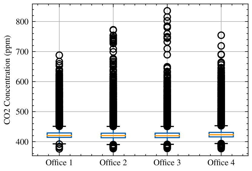
(a) Indoor $CO_{2}$ Concentration ($CO_{2\_{in}}$)

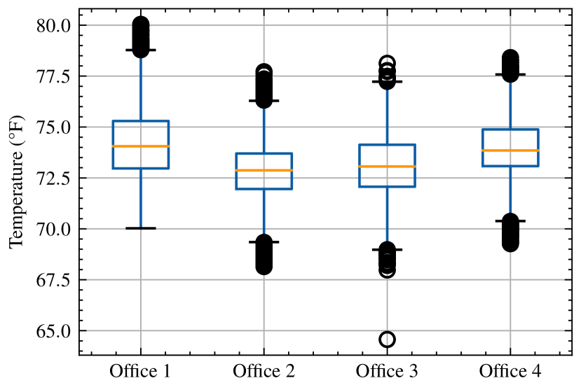
(b) Indoor Temperature ($T_{in}$)

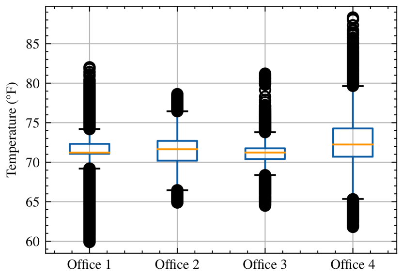
(c) Outdoor Temperature ($T_{out}$)

Figure 1. Comparative environmental conditions across four office spaces.

Transformer models by Vaswani et al. (2017) (Vaswani et al., 2017), have revolutionized time series forecasting through their innovative use of self-attention mechanisms, enabling the model to focus selectively on relevant parts of the input. This model’s parallelizable architecture significantly enhances its efficiency in handling large datasets. There are also newer models based on transformers such as PatchTST (Nie et al., 2022), Informer (Zhou et al., 2021), and Autoformer (Wu et al., 2021).

Furthermore, Informer model by Zhou et al. (2021) (Zhou et al., 2021), which addresses the quadratic time complexity and memory usage inherent in traditional Transformer models, introduces the ProbSparse self-attention mechanism, a distilling operation, and a generative decoder to manage long-sequence time-series forecasting effectively. This model demonstrates a marked improvement in prediction capabilities for long-sequence forecasting tasks by mitigating the limitations of the encoder-decoder architecture.

The FEDformer model, introduced by Zhou et al. (2022) (Zhou et al., 2022), represents another advancement in time series forecasting by integrating Transformer architecture with seasonal-trend decomposition. This hybrid approach enables the FEDformer to capture both the global trends and the intricate details within the time series data. By leveraging the sparsity in the frequency domain, FEDformer achieves enhanced efficiency and effectiveness in long-term forecasting, outpacing conventional Transformer models in both performance and computational efficiency.

In contrast, the Autoformer model by Wu et al. (2021) (Wu et al., 2021) incorporates an Auto-Correlation mechanism and a novel series decomposition strategy within its architecture. This approach allows the Autoformer to dissect and analyze complex time series data, focusing on seasonal patterns while progressively incorporating trend components. This model’s unique design facilitates a deeper understanding of temporal dependencies, particularly in sub-series levels, thereby offering a robust solution for long-term forecasting challenges.

In addition, the introduction of a linear decomposition model, Dlinear, by Zeng et al. (2023) (Zeng et al., 2023) challenges the prevailing dominance of Transformer-based models in long-term time series forecasting. By simplifying the model to focus on linear relationships within the data, Dlinear astonishingly surpasses more complex models in performance. This revelation underscores the potential of minimalistic approaches in extracting temporal relationships effectively, thereby questioning the necessity of complex architectures for certain forecasting tasks.

Moreover, the Modern Temporal Convolutional Network (ModernTCN) by Luo et al. (2024) (Luo and Wang, 2024), leverages convolutional operations to model temporal dependencies. ModernTCN employs dilated convolutions, residual connections, and layer normalization, resulting in a highly effective time series forecasting model with reduced computational overhead. However, ModernTCN may suffer from limited representation capabilities due to its lightweight backbone, potentially leading to inferior performance in certain tasks.

Additionally, SegRNN by Lin et al. (2023) (Lin et al., 2023) revisits RNN-based methods by introducing segment-wise iterations and parallel multi-step forecasting. These techniques reduce the number of recurrent steps and enhance forecasting accuracy and inference speed, making SegRNN a highly efficient tool for long-term time series forecasting. Despite these improvements, SegRNN can be constrained by the inherent limitations of RNNs, such as vanishing gradients and difficulty in capturing long-term dependencies.

Lastly, TiDE by Das et al. (2023) (Das et al., 2023) combines the strengths of linear models and multi-layer perceptrons (MLPs). TiDE’s dense encoder architecture captures both linear and nonlinear dependencies in time series data, offering robust performance without the excessive computational demands of more complex models like transformers. Nonetheless, TiDE can struggle with modeling non-linear dependencies and may face challenges when dealing with complex covariate structures.

Our DSSRNN model builds upon decomposition techniques used in Dlinear, Autoformer, and Fedformer, while significantly enhancing computational efficiency. By optimizing its architecture, DSSRNN achieves faster training and inference times than leading transformer-based models, making it particularly suitable for real-time applications.

3. Decomposition State-Space Recurrent Neural Network (DSSRNN)

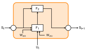
Figure 2. State-Space Recurrent Neural Network (SS-RNN).

Our proposed model, the Decomposition State-Space Recurrent Neural Network (DSSRNN), builds upon two innovative physics-infused ML models: the State-Space Recurrent Neural Network (SS-RNN), Figure 2, and its advanced iteration, the Decomposition State-Space Recurrent Neural Network (DSSRNN), Figure 3. The SS-RNN framework synergizes the robustness of state-space physics with the flexibility of recurrent neural networks, while the DSSRNN employs moving-average decomposition to filter out high-frequency noise inherent in temporal datasets.

Finally, note that DSSRNN, uses the same framework for the imputation as well as the prediction tasks. This dual functionality underscores the versatility of our model, providing a cohesive approach to managing and forecasting time series data.

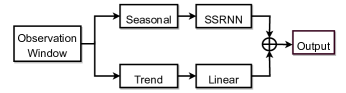
Figure 3. Decomposition State-Space Recurrent Neural Network (DSSRNN).

3.1. Data

In our study, we utilized data from Lawrence Berkeley National Laboratory’s Building 59 in California, covering the period from August 19, 2019, to December 31, 2021. This unique indoor air quality (IAQ) dataset, notable for its rarity due to the generally limited availability of comprehensive data in this area, contains 20,760 data points from office settings. It encompasses hourly indoor $CO_{2}$ measurements along with other crucial environmental variables—a collection of data infrequently encountered in existing studies. The location of each office numbered 44, 45, 62, and 68 within the building is detailed in a map provided in (Luo et al., 2022), offering contextual insight into the data collection environment. A key aspect of our research is the prediction of indoor $CO_{2}$ concentration ($CO_{2\_in}$), using five current environmental variables such as current indoor $CO_{2}$ levels, time of day (Hour), day of the week (Num_Week), and both indoor and outdoor temperatures ($T_{\text{in}}$ and $T_{\text{out}}$) (Mohammadshirazi et al., 2022, 2023).

In Figure 1, we present a comprehensive depiction of the environmental conditions across four different office settings through the analysis of indoor temperature, outdoor temperature, and indoor $CO_{2}$ concentration. The subfigure 1(a) focuses on the indoor $CO_{2}$ concentration levels. Across all offices, the median $CO_{2}$ concentration is consistent, indicating a general adherence to acceptable IAQ standards. However, the presence of numerous high outliers in each office suggests episodic events where the $CO_{2}$ levels exceed typical ranges. These instances could potentially be linked to variable occupancy levels, inconsistent operation of ventilation systems, or activities within the offices that temporarily increase $CO_{2}$ production.

The indoor temperature, illustrated in the subfigure 1(b), reveals a notable variance between offices. Office 1 exhibits a broad temperature range with several high outliers, indicative of sporadic deviations from the norm, which could be attributed to intermittent HVAC system performance or external factors affecting the indoor climate. In contrast, Offices 2 and 3 display a narrower interquartile range, suggesting a more consistent application of temperature control measures. Office 4, while also showing a relatively stable temperature range, has more outliers on the lower end, pointing to occasional dips in the indoor temperature.

The subfigure 1(c) captures the outdoor temperature conditions for each office location. Offices 1, 3, and 4 show a wider range of temperature values, which may reflect either a larger variance in outdoor climatic conditions or a more extended period of data capture. Office 2 demonstrates tighter temperature controls with minimal outliers, suggesting either less climatic variability or more effective mitigation of outdoor temperature fluctuations. Overall, the multitude of data eliminates the statistical biases, and the variety of the data supports the training of a robust model.

Analysis of the dataset reveals the presence of missing values, as detailed in Table 1, corresponding to the period from January 2020 to April 2020. The missing data is imputed, and appropriate sections of the dataset are selected for training, testing, and validation to maintain the integrity of our analysis. The upcoming section elaborates on this method and its significance in our research.

Input Variables	$CO_{2-in}$	$T_{in}$	$T_{out}$
Office1	2,823 (13.6%)	3,027 (14.6%)	2,823 (13.6%)
Office2,3,4	2,823 (13.6%)	2,823 (13.6%)	2,823 (13.6%)

Table 1. Input Variables with Missing Entries for Predicting Indoor $CO_{2}$ Concentrations across Four Office Environments

3.2. Imputation Methods

In this section, we explore the imputation methods utilized to address the challenge of missing data within our datasets. Table 1 provides a detailed examination of the data absence across various input variables collected from four distinct office environments, spanning from January 2020 to April 2020. To effectively manage this dataset, we segregated it into training, validation, and testing subsets, with all instances of missing data allocated to the testing subset. Our proposed DSSRNN model is uniquely designed to tackle both prediction and imputation tasks using the same architecture. It evaluates performance metrics such as Mean Squared Error (MSE) and Mean Absolute Error (MAE) during the validation phase to accurately impute missing values. Given our development of the DSSRNN model to serve dual purposes—both prediction and imputation—using a unified architecture, we will delve into a comprehensive explanation of our DSSRNN model in the subsequent section dedicated to prediction.

3.3. Prediction Methods

In the prediction section of the paper, we delve into the architecture of our advanced model, the Decomposition State-Space Recurrent Neural Network (DSSRNN). This section outlines the foundational State-Space Recurrent Neural Network (SS-RNN) structure and its extension into the DSSRNN model, which incorporates decomposition techniques for enhanced prediction capabilities. We will first elaborate on the SS-RNN architecture, explaining its design and how it integrates the robustness of physic-based and state-space models with the adaptability of recurrent neural networks. Subsequently, we will discuss the DSSRNN and how it utilizes decomposition to refine the prediction of time series data, including the identification and forecasting of outlier events. This approach underpins the robustness of our model in predicting critical, rare events within the datasets, which we illustrate through a comparative analysis with leading models in the domain.

3.3.1. State-Space Recurrent Neural Networks (SS-RNN)

The State-Space Recurrent Neural Network (SS-RNN) architecture represents a novel blend of traditional state-space models with the dynamic capabilities of recurrent neural networks (RNNs). At its core, SS-RNN aims to model time series data by capturing both the underlying physical processes and temporal dependencies. This is achieved through a combination of state variables that embody the physical state of the system and RNN layers that process sequential data, allowing for the integration of prior knowledge and temporal context. The SS-RNN architecture is designed to efficiently handle the flow of information through time, making it particularly adept at predicting complex dynamics in time series data, such as those encountered in IAQ monitoring.

The transformation from physic to ML equations begins with the foundational state-space representation of indoor $CO_{2}$ dynamics (Persily, 2022), as shown in Equation 1. This equation models the temporal change in indoor $CO_{2}$ concentration by relating it to variables that capture both the physical characteristics of the environment and the dynamics of $CO_{2}$ exchange. Specifically, the mass flow rate $\dot{m}$ reflects the air exchange due to ventilation, represented by $\frac{\dot{m}}{\rho V}\times CO_{2\_out}$, $\rho$ signifies air density, $V$ stands for the volume of the indoor space, and $M_{t}$ represents the internal generation of $CO_{2}$, such as those generated by occupants or appliances within the space. The variable $CO_{2\_out}$, meanwhile, captures the concentration of $CO_{2}$ outside the building. Together, these variables form the basis of our state-space approach, setting the stage for its translation into an ML framework.

(1) $$\frac{\partial}{\partial t}CO_{2\_in}=\frac{\dot{m}}{\rho V}(CO_{2\_out}-CO_{2\_in})+\frac{M_{t}}{\rho}$$

Equation 2 is where the conversion to an ML framework takes place. The term $A$ represents the state matrix, encapsulating the system dynamics, and $B$ the input matrix, incorporating external influences. These matrices interact with the state vector $S_{t}$ (Equation 3) and input vector $U_{t}$ (Equation 4) to form a discretized version of the physics-based model, respectively. This interaction is key to defining the subsequent state vector $S_{t+1}$ and the differential state change $dS_{t+1}$. These state vectors, embedded within the ML architecture, allow neural networks to approximate the intricate relationships found within the dataset. The continuous state update from $S_{t}$ to $S_{t+1}$ (Equation 3), facilitated by the differential state $dS_{t+1}$, is a discrete analog of the physical process. This reformulation allows us to leverage the power of neural networks to approximate the complex relationships within the data, retaining the interpretability and structure provided by the physical model.

(2) $$\underbrace{\frac{\partial}{\partial t}(CO_{2\_in})}_{dS_{t+1}}=\underbrace{{-}\frac{\dot{m}}{\rho V}}_{A}\times\underbrace{CO_{2\_in}}_{S_{t}}+\{\underbrace{\frac{\dot{m}}{\rho V}\times{CO_{2\_out}}+\frac{M_{t}}{\rho}}_{B{\times}{U_{t}}}\}$$

(3) $$S_{t+1}\leftarrow{CO_{2\_in_{t+1}}},S_{t}\leftarrow{CO_{2\_in_{t}}}$$

(4) $$U_{t}\leftarrow{CO_{2\_in_{t}}},{Hour}_{t},T_{in_{t}},T_{out_{t}},Num\_week_{t}$$

The SS-RNN model, presented in Figure 2, is meticulously crafted to process inputs within each discrete time step. The model assimilates the current state vector $S_{t}$ and the input vector $U_{t}$ to advance its internal state. The transformation of $S_{t}$ alongside $U_{t}$ is governed by a nonlinear function $F_{1}$, resulting in the interim state change $dS_{t+1}$, as shown in equation 5. This intermediate state is then sculpted by another nonlinear function $F_{2}$, culminating in the updated state $S_{t+1}$ (Equation 6). Weight matrices $W_{dSS}$ and $W_{dSU}$, alongside bias vectors $b_{dSS}$ and $b_{dSU}$, underpin this evolution, modulating the influence of past and present information and embedding non-linearity via ReLU activation functions, denoted as $F_{1}$ and $F_{2}$ (see equation 7).

Based on Figure 2 representation, the SS-RNN ML model state space and its changes are updated as follows:

(5) $$dS_{t+1}\leftarrow F_{1}(S_{t}\times W_{dSS}+b_{dSS}+U_{t}\times W_{dSU}+b_{dSU})$$

(6) $$S_{t+1}\leftarrow F_{2}(S_{t}+dS_{t+1})$$

(7) $$S_{t+1}\leftarrow F_{2}(S_{t}+F_{1}(S_{t}\times W_{dSS}+b_{dSS}+U_{t}\times W_{dSU}+b_{dSU})$$

It should be noted that the equation referenced in 1, while primarily developed for modeling $CO_{2}$, can be adapted to encompass a variety of indoor pollutants such as $NO_{2}$, $O_{3}$, $PM_{1}$, $PM_{2.5}$, and $PM_{10}$. This adaptation necessitates modifying the generation term $M_{t}$ for each specific pollutant’s source strength and incorporating particular deposition or removal processes. Such modifications allow the SS-RNN model to extend its applicability across a range of indoor pollutants, demonstrating its versatility in different environmental conditions. In the following subsection, we will expound on the intricacies of the Decomposition State-Space Recurrent Neural Network (DSSRNN) and its implementation for enhanced predictive performance.

3.3.2. Decomposition State-Space Recurrent Neural Networks (DSSRNN)

DSSRNN architecture advances the SS-RNN framework by incorporating decomposition techniques to dissect and model the temporal data into trend and seasonal components by incorporating a decomposition mechanism to capture and model both global and local temporal structures within the data. Specifically, the trend component, represented as a moving average calculated over a 24-hour window, captures the global patterns. In contrast, the seasonal component—obtained by subtracting this trend from the observation window—reflects local fluctuations. As depicted in Figure 3, the observation window provides input to two parallel pathways: one for isolating seasonal patterns processed by the SS-RNN, and another for delineating the trend via a linear model. The outputs of these pathways are then synergistically combined to yield the final output, capturing both the nuanced cyclicity and underlying directional movement in the data. This bifurcation allows the DSSRNN to adeptly handle the intricacies of time series forecasting, enhancing its ability to identify and predict complex patterns influenced by both long-term trends and short-term seasonal variations.

3.3.3. Predicting outlier events

	Threshold	Number of events	Percentage
		Training/(Testing)	Training/(Testing)
Office 1	451.12	1112/(268)	7.70%/(6.46%)
Office 2	450.84	1019/(260)	7.06%/(6.26%)
Office 3	450.75	1175/(292)	8.14%/(7.03%)
Office 4	453.05	928/(271)	6.43%/(6.53%)

Table 2. Comparative analysis across training and testing datasets between the number of high-concentration CO₂ events and the corresponding percentage of data points for each office alongside their third quartile threshold

In order to demonstrate the robustness of our model in predicting outlier events within the $CO_{2}$ data, we employ a binary classification approach based on the box-and-whisker plot method. Specifically, $CO_{2}$ measurements above the upper whisker—calculated as $Q_{3}+1.5\times IQR$ where $Q_{3}$ is the third quartile and $IQR$ is the interquartile range—are classified as outliers and encoded as ’1’, while non-outliers are assigned ’0’ (See the threshold value for each office in Table 2. This binary transformation allows us to specifically focus on the prediction of outlier occurrences. We then compare the performance of our model in predicting these binary outcomes against SoTA models, showcasing our model’s capability to identify significant deviations in air quality. The number of outlier events detected for each office is systematically cataloged in Table 2. The comparative results and analysis are presented in detail in the Result section of the paper.

Methods	Metric	Office 1 (44)				Office 2 (45)				Office 3 (62)				Office 4 (68)
		96	192	336	720	96	192	336	720	96	192	336	720	96	192	336	720
FEDformer	MSE	1.062	1.208	1.166	1.186	1.008	1.054	0.974	1.143	1.070	1.076	0.944	0.891	1.030	1.137	1.123	0.878
	MAE	0.740	0.792	0.770	0.786	0.723	0.740	0.709	0.768	0.745	0.749	0.709	0.691	0.750	0.793	0.788	0.687
Transformer	MSE	0.528	0.599	0.651	0.643	0.421	0.555	0.572	0.553	0.471	0.636	0.500	0.534	0.528	0.529	0.713	0.581
	MAE	0.497	0.536	0.566	0.565	0.461	0.539	0.533	0.525	0.448	0.522	0.465	0.477	0.497	0.490	0.566	0.525
Autoformer	MSE	0.619	0.667	0.767	0.704	0.586	0.613	0.603	0.599	0.537	0.607	0.934	0.620	0.648	0.729	1.193	0.645
	MAE	0.598	0.583	0.648	0.598	0.556	0.557	0.561	0.561	0.527	0.555	0.698	0.555	0.591	0.629	0.809	0.586
Informer	MSE	0.531	0.567	0.514	0.625	0.523	0.555	0.549	0.593	0.522	0.535	0.510	0.529	0.576	0.577	0.522	0.520
	MAE	0.508	0.527	0.482	0.553	0.504	0.519	0.509	0.538	0.477	0.471	0.465	0.484	0.503	0.516	0.502	0.492
PatchTST	MSE	0.431	0.484	0.497	0.526	0.410	0.461	0.475	0.496	0.382	0.442	0.456	0.491	0.422	0.484	0.501	0.516
	MAE	0.460	0.485	0.489	0.504	0.452	0.476	0.480	0.489	0.420	0.453	0.460	0.473	0.453	0.484	0.491	0.495
TiDE	MSE	0.491	0.521	0.557	0.612	0.481	0.526	0.573	0.648	0.391	0.404	0.411	0.436	0.507	0.536	0.561	0.613
	MAE	0.471	0.489	0.502	0.535	0.473	0.490	0.510	0.549	0.415	0.422	0.432	0.447	0.488	0.500	0.513	0.541
ModernTCN	MSE	0.491	0.586	0.586	0.605	0.460	0.549	0.549	0.551	0.428	0.522	0.531	0.567	0.473	0.586	0.615	0.599
	MAE	0.482	0.525	0.526	0.529	0.474	0.516	0.513	0.512	0.445	0.490	0.495	0.506	0.487	0.541	0.556	0.543
Linear	MSE	0.452	0.503	0.508	0.536	0.426	0.477	0.483	0.502	0.397	0.450	0.463	0.497	0.436	0.495	0.507	0.519
	MAE	0.475	0.499	0.501	0.509	0.462	0.487	0.489	0.498	0.438	0.466	0.475	0.488	0.469	0.498	0.504	0.502
Nlinear	MSE	0.513	0.615	0.611	0.621	0.476	0.569	0.569	0.569	0.448	0.547	0.557	0.585	0.494	0.614	0.642	0.616
	MAE	0.500	0.545	0.542	0.542	0.485	0.527	0.523	0.522	0.462	0.506	0.510	0.518	0.501	0.556	0.571	0.554
DLinear	MSE	0.454	0.500	0.504	0.535	0.422	0.474	0.479	0.499	0.392	0.446	0.458	0.494	0.429	0.491	0.503	0.517
	MAE	0.475	0.497	0.498	0.508	0.459	0.485	0.486	0.496	0.434	0.463	0.472	0.485	0.464	0.495	0.501	0.501
VanillaRNN	MSE	0.452	0.508	0.498	0.544	0.411	0.463	0.499	0.526	0.399	0.439	0.477	0.477	0.432	0.513	0.485	0.524
	MAE	0.470	0.512	0.493	0.505	0.450	0.465	0.495	0.508	0.428	0.457	0.452	0.471	0.462	0.499	0.481	0.501
GRU	MSE	0.451	0.490	0.528	0.558	0.512	0.542	0.518	0.586	0.459	0.453	0.481	0.504	0.467	0.523	0.549	0.526
	MAE	0.459	0.474	0.483	0.503	0.498	0.514	0.502	0.546	0.446	0.456	0.472	0.476	0.484	0.508	0.520	0.503
LSTM	MSE	0.456	0.507	0.538	0.548	0.422	0.494	0.538	0.538	0.420	0.427	0.447	0.479	0.454	0.556	0.584	0.516
	MAE	0.456	0.480	0.499	0.497	0.453	0.500	0.526	0.529	0.438	0.443	0.457	0.472	0.477	0.520	0.536	0.494
SegRNN	MSE	0.491	0.564	0.554	0.576	0.483	0.571	0.560	0.544	0.453	0.549	0.548	0.580	0.509	0.600	0.630	0.613
	MAE	0.488	0.523	0.520	0.530	0.486	0.524	0.518	0.513	0.462	0.506	0.509	0.521	0.504	0.548	0.566	0.558
SSRNN	MSE	0.393	0.444	0.450	0.477	0.370	0.418	0.424	0.444	0.342	0.391	0.403	0.438	0.378	0.437	0.448	0.460
	MAE	0.416	0.440	0.442	0.450	0.406	0.428	0.430	0.439	0.382	0.406	0.416	0.429	0.410	0.439	0.444	0.443
DSSRNN	MSE	0.378	0.428	0.434	0.463	0.353	0.403	0.409	0.429	0.320	0.375	0.388	0.425	0.359	0.421	0.433	0.445
	MAE	0.401	0.426	0.428	0.437	0.390	0.415	0.416	0.426	0.362	0.392	0.402	0.416	0.394	0.424	0.431	0.430

Table 3. Comparative Forecasting Performance: This table presents the MSE and MAE across forecasting horizons (T) of 96, 192, 336, 720 for four office environments, with input sequence length L=96. Bold figures indicate the best overall performance, while underlined figures show the top results for transformer-based, MLP-based, and linear-based models.

4. Experiments

In the results section of our paper, we evaluate the DSSRNN’s performance using the robust NVIDIA A100 GPU at the Ohio Supercomputer Center (OSC) . The forthcoming subsections will present a detailed account of the model’s imputation and prediction capabilities, each scrutinized through rigorous experimentation. These findings will illustrate the DSSRNN’s strengths in accurately forecasting and handling missing data within the context of indoor air quality assessment.

4.1. Imputation Analysis

Method	Metrics	Office 1	Office 2	Office 3	Office 4
DSSRNN	MSE	0.357	0.180	0.217	0.373
	MAE	0.375	0.284	0.293	0.367
DLinear	MSE	0.383	0.199	0.233	0.397
	MAE	0.393	0.299	0.304	0.382
SAITS	MSE	1.079	0.956	0.922	0.954
	MAE	0.686	0.701	0.669	0.710

Table 4. Comparative Imputation Performance: MSE and MAE for DSSRNN, Dlinear, and SAITS across four office environments with a prediction sequence length (T) of 1. Bold figures highlight the top performance for each metric.

In the results section outlined in Section 3.2, we present a comprehensive evaluation of our DSSRNN model in comparison with other imputation methods. The evaluation, focused on the imputation accuracy, is crucial given the presence of missing values documented in Table 1. Our approach, embodied by the DSSRNN model, is meticulously compared against alternative methodologies, including DLinear (a linear-based model) (Zeng et al., 2023) and SAITS (a self-attention-based model) (Du et al., 2023), in terms of their ability to handle missing data effectively. The comparative analysis, as presented in Table 4, demonstrates the superior performance of DSSRNN in minimizing both MSE and MAE metrics. For office 1, DSSRNN attains an MSE of 0.357 and an MAE of 0.375, which are the lowest among the methods compared. This pattern of outperformance continues across Office 2, Office 3, and Office 4, with DSSRNN maintaining the lead in minimizing error metrics, signifying its robustness in dealing with incomplete data.

DLinear, while being a robust model based on linear methodologies, exhibits higher MSE and MAE metrics compared to DSSRNN. This indicates that despite its strengths, DLinear encounters limitations when processing datasets with missing information. In contrast, DSSRNN, which transcends the linear approach of DLinear, captures complex temporal dynamics through a deeper understanding of the data’s underlying processes, thereby offering a more comprehensive representation of patterns. However, SAITS, despite embodying the forefront of self-attention-based imputation techniques, falls short of DSSRNN’s performance, as evidenced by its higher MSE and MAE figures. This disparity highlights potential challenges SAITS faces in effectively managing the complexities associated with missing data.

Through this evaluation, DSSRNN’s advanced architecture proves to be instrumental in accurately learning and imputing data patterns, outshining the state-of-the-art models that were specifically chosen for their superior performance in their respective categories. The bold metrics in Table 4 underscore DSSRNN’s exceptional capability to reconstruct missing data with unparalleled precision, solidifying its standing as the leading imputation model for tackling data sparsity in various analytical applications.

4.2. Prediction Analysis

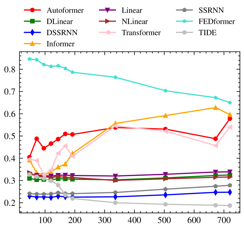
(a) 24 steps - Office 1

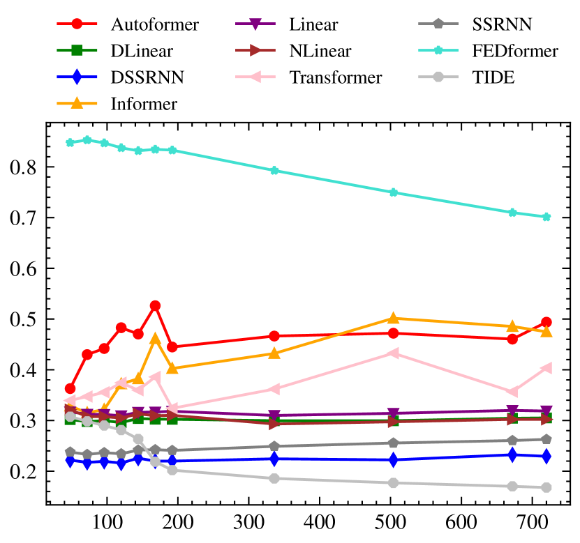
(b) 24 steps - Office 2

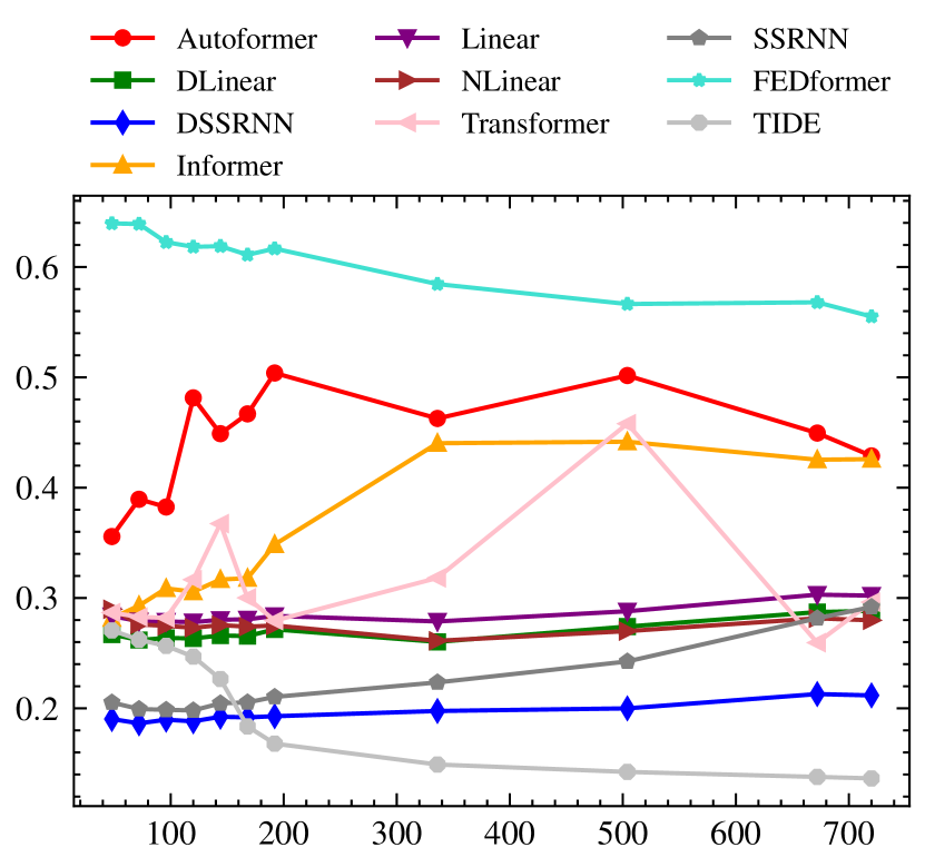
(c) 24 steps - Office 3

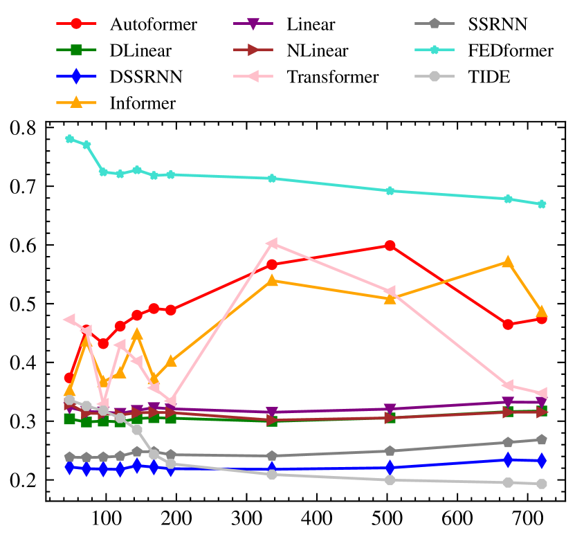
(d) 24 steps - Office 4

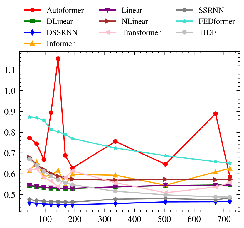
(e) 720 steps - Office 1

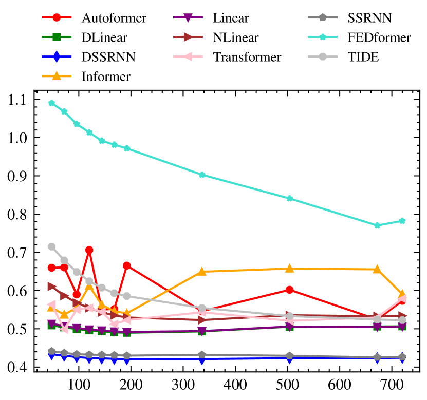
(f) 720 steps - Office 2

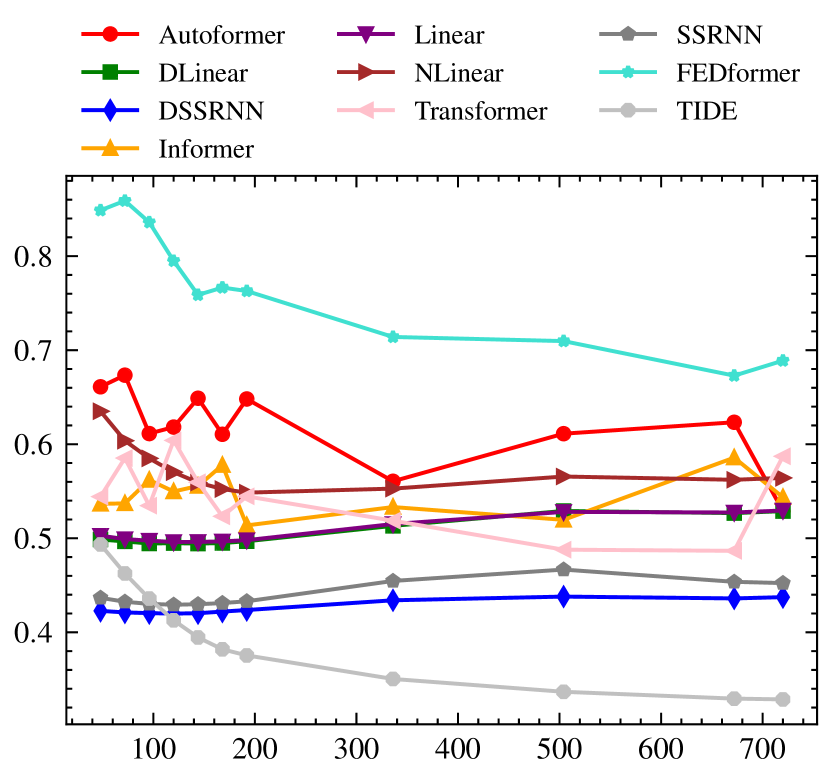
(g) 720 steps - Office 3

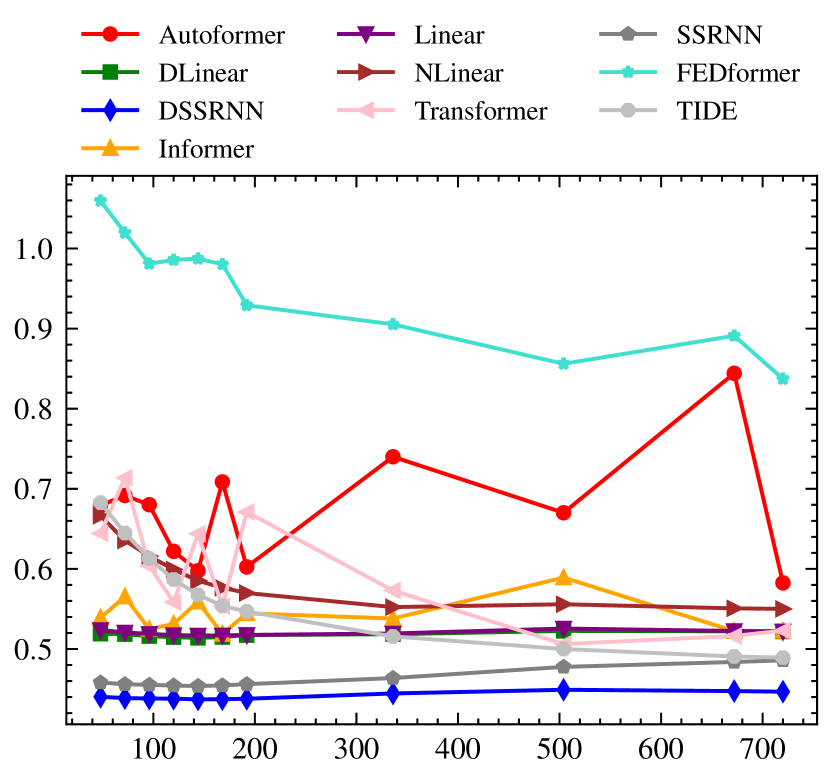
(h) 720 steps - Office 4

Figure 4. Comparative MSE Analysis for Forecasting Models: Illustrated here are the MSE metrics for models with varying look-back window sizes for both long-term (e.g., 720 steps) and short-term (e.g., 24 steps) forecasting. The Y-axis measures MSE, while the X-axis represents the look-back window size, highlighting performance across four offices.

In the comprehensive assessment of forecasting methodologies detailed in Table 3 eclipsing a spectrum of advanced models. Our experimental procedures, aligned with the benchmarks set by Zeng et al. (2023) (Zeng et al., 2023), ensured a balanced comparison across the forecast horizons T=96, 192, 336, 720, catering to the input length for long-term time series forecasting. DSSRNN consistently delivered the most accurate forecasts, achieving the lowest MSE and MAE values at all forecast lengths and across all office environments. For example, at the shortest horizon (T=96) in Office1, DSSRNN reported an MSE of 0.378 and an MAE of 0.401, establishing its proficiency in capturing intricate temporal dynamics. Among the linear-based models, Dlinear showed commendable performance, especially at medium to long forecast horizons, marking it as the best within its category. Within the transformer-based models, ’Transformer’ excelled at the shortest horizon (T=96), while ’Informer’ demonstrated its strength at extended lengths (T=192, 336, and 720), adept at handling long-range data dependencies.

Our research into short-term time series forecasting evaluates the DSSRNN model across various sequence lengths ranging from 24 to 720-time steps, examining its performance in four office settings for both short-term (e.g., 24-time steps) and long-term forecasting (e.g., 720-time steps). As detailed in Figure 4, DSSRNN performs greatly in most settings and although TIDE has a superior accuracy in some cases, considering its high computational cost, our model can be seen as a better choice, striking a balance between computational cost and accuracy. These findings underscore DSSRNN’s adaptability to various forecasting horizons and its transformative potential in time series analysis.

Classification

Performance
Metrics	Model	Office 1	Office 2	Office 3	Office 4
True Positive	DSSRNN	192	209	234	218
	DLinear	181	189	223	203
	PatchTST	179	178	219	207
False Positive	DSSRNN	84	80	46	67
	DLinear	137	111	67	95
	PatchTST	98	99	57	98
True Negative	DSSRNN	3,799	3,811	3,813	3,807
	DLinear	3,757	3,780	3,792	3,785
	PatchTST	3,785	3,792	3,802	3,782
False Negative	DSSRNN	76	51	46	73
	DLinear	87	71	69	68
	PatchTST	89	82	73	64
Accuracy	DSSRNN	96.15%	96.84%	97.52%	96.96%
	DLinear	94.87%	95.62%	96.72%	96.07%
	PatchTST	95.50%	95.64%	96.87%	96.10%
Precision	DSSRNN	69.57%	72.32%	84.63%	74.91%
	DLinear	58.96%	63.00%	76.90%	68.12%
	PatchTST	64.62%	64.26%	79.35%	67.87%
Recall	DSSRNN	71.64%	80.38%	80.48%	80.44%
	DLinear	67.54%	72.69%	76.37%	74.91%
	PatchTST	66.79%	68.46%	75.00%	76.38%
F1 Score	DSSRNN	70.59%	76.14%	82.02%	77.58%
	DLinear	62.96%	67.50%	76.63%	71.35%
	PatchTST	65.69%	66.29%	77.11%	71.88%

Table 5. Comparative analysis of model performance metrics for $CO_{2}$ concentration event classification over T = 96.

In an effort to further comprehend the regression capabilities of our DSSRNN model, we transformed the regression task into a classification problem, as meticulously explained in Section 3.3.3. The results of this transformation are depicted in Table 5, where we delineate the thresholds set for event detection, the count of events, and their respective percentages for each office environment.

The classification approach allows us to dissect the model’s performance in distinguishing between high-concentration and normal event occurrences. While the DLinear model exhibits commendable recall for high-concentration events—likely a result of its decomposition capability, breaking down time series into seasonal and trend components—the Autoformer model shows a preference for normal events. This tendency is attributed to its Transformer-based architecture, which is proficient in modeling long-range dependencies within the data.

Notwithstanding the strengths displayed by DLinear and Autoformer in their respective domains, the DSSRNN model demonstrates a clear overarching superiority. It transcends the typical decomposition approach by integrating state space physics concepts, offering a profound understanding of the dynamics of the time series data. DSSRNN consistently maintains higher True Positive rates alongside lower False Positive rates, indicating an adeptness at correctly identifying events while minimizing false alarms—a critical aspect for real-world applications. The True Negative rate is also the highest for DSSRNN, reflecting its strong discriminative power in differentiating non-events. Precision and Recall are metrics where DSSRNN distinctly outshines its counterparts. The model’s precision is indicative of the reliability and exactitude of its predictions, while the higher recall rates—especially for high-concentration events—demonstrate an increased sensitivity and a lower propensity to overlook significant events.

Computational Efficiency

Method	MACs	Parameter	Time	Memory
DSSRNN	0.11G	408.21K	0.58ms	437MiB
DLinear	0.04G	139.7K	0.15ms	196MiB
TiDE	1.09G	2.69M	32.87ms	1011MiB
PatchTST	4.79G	18.21M	14.03ms	2033MiB
Transformer	4.03G	13.61M	10.31ms	1740MiB
Informer	3.93G	14.39M	18.96ms	1105MiB
FEDformer	4.41G	20.68M	15.58ms	1183MiB

Table 6. Comparative analysis of computational efficiency between DSSRNN, DLinear, and various transformer-based models, evaluated on the Office #1 air quality dataset with input sequence length $L=96$ and prediction sequence length $T=720$. Metrics include multiply-accumulate operations (MACs), model parameters, average inference time over five runs, and memory usage.

In our comparative analysis, delineated in Table 6, we scrutinize the computational efficiency of our proposed DSSRNN model compared to DLinear and a suite of Transformer-based architectures. This evaluation is predicated on the Office #1 air quality dataset, adopting an input sequence length $L=96$ and a prediction sequence length $T=720$. The criteria for this comparison encompass multiply-accumulate operations (MACs), the aggregate number of model parameters, the average inference time over a quintet of runs, and the requisite memory allocation during computational processes.

DLinear distinguished itself as the most computationally efficient model, demanding the least computational resources with a mere 0.04G MACs and minimal memory usage of 196MiB, alongside a remarkable average inference speed of 0.15ms. This exceptional efficiency renders it particularly advantageous for resource-constrained settings. Close on its heels, DSSRNN stands as the second most efficient model, consuming slightly more resources at 0.11G MACs and 437MiB of memory but still delivering a swift inference time of 0.58ms, validating its efficacy.

5. Conclusion and Future Work

In this study, the Decomposition State-Space Recurrent Neural Network (DSSRNN) was introduced, integrating physics and state-space methodologies to adeptly impute missing data and forecast indoor air pollutant concentrations. The architecture of this model is designed for computational efficiency, surpassing the performance of conventional transformer-based models. The DSSRNN has shown exceptional proficiency, outperforming established benchmark models in both MSE and MAE, which highlights its potential for accurate regression and classification predictions and reliable data imputation. The success of the DSSRNN paves the way for the application of physics-informed machine learning models in environmental data analysis and potentially in other predictive domains.

For future work, we aim to apply the integration of physics-based concepts and state-space models with ML techniques to broader domains, such as the modeling and forecasting of energy consumption in buildings. This will involve analyzing usage patterns alongside external factors like weather conditions. Additionally, we will explore the optimization of climate control systems, focusing on heating, ventilation, and air conditioning to adapt efficiently to environmental variations. This expansion will harness the DSSRNN model’s strengths in addressing both indoor and outdoor pollutant dynamics and energy efficiency challenges.

References

- (1)
- Bansal et al. (2021) Parikshit Bansal, Prathamesh Deshpande, and Sunita Sarawagi. 2021. Missing value imputation on multidimensional time series. arXiv preprint arXiv:2103.01600 (2021).
- Barra et al. (2020) Silvio Barra, Salvatore Mario Carta, Andrea Corriga, Alessandro Sebastian Podda, and Diego Reforgiato Recupero. 2020. Deep learning and time series-to-image encoding for financial forecasting. IEEE/CAA Journal of Automatica Sinica 7, 3 (2020), 683–692.
- Blázquez-García et al. (2021) Ane Blázquez-García, Angel Conde, Usue Mori, and Jose A Lozano. 2021. A review on outlier/anomaly detection in time series data. ACM Computing Surveys (CSUR) 54, 3 (2021), 1–33.
- Bochenek and Ustrnul (2022) Bogdan Bochenek and Zbigniew Ustrnul. 2022. Machine learning in weather prediction and climate analyses—applications and perspectives. Atmosphere 13, 2 (2022), 180.
- Cao et al. (2018) Wei Cao, Dong Wang, Jian Li, Hao Zhou, Lei Li, and Yitan Li. 2018. Brits: Bidirectional recurrent imputation for time series. Advances in neural information processing systems 31 (2018).
- Casale et al. (2018) Francesco Paolo Casale, Adrian Dalca, Luca Saglietti, Jennifer Listgarten, and Nicolo Fusi. 2018. Gaussian process prior variational autoencoders. Advances in neural information processing systems 31 (2018).
- Che et al. (2018) Zhengping Che, Sanjay Purushotham, Kyunghyun Cho, David Sontag, and Yan Liu. 2018. Recurrent neural networks for multivariate time series with missing values. Scientific reports 8, 1 (2018), 6085.
- Chen et al. (2023) Zhe Chen, Fu Xiao, Fangzhou Guo, and Jinyue Yan. 2023. Interpretable machine learning for building energy management: A state-of-the-art review. Advances in Applied Energy (2023), 100123.
- Das et al. (2023) Abhimanyu Das, Weihao Kong, Andrew Leach, Shaan Mathur, Rajat Sen, and Rose Yu. 2023. Long-term forecasting with tide: Time-series dense encoder. arXiv preprint arXiv:2304.08424 (2023).
- Du et al. (2023) Wenjie Du, David Côté, and Yan Liu. 2023. Saits: Self-attention-based imputation for time series. Expert Systems with Applications 219 (2023), 119619.
- Emmanuel et al. (2021) Tlamelo Emmanuel, Thabiso Maupong, Dimane Mpoeleng, Thabo Semong, Banyatsang Mphago, and Oteng Tabona. 2021. A survey on missing data in machine learning. Journal of Big Data 8, 1 (2021), 1–37.
- Fortuin et al. (2020) Vincent Fortuin, Dmitry Baranchuk, Gunnar Rätsch, and Stephan Mandt. 2020. Gp-vae: Deep probabilistic time series imputation. In International conference on artificial intelligence and statistics. PMLR, 1651–1661.
- Friedland (2012) Bernard Friedland. 2012. Control system design: an introduction to state-space methods. Courier Corporation.
- Fu et al. (2022) Daniel Y Fu, Tri Dao, Khaled K Saab, Armin W Thomas, Atri Rudra, and Christopher Ré. 2022. Hungry hungry hippos: Towards language modeling with state space models. arXiv preprint arXiv:2212.14052 (2022).
- Kashinath et al. (2021) Karthik Kashinath, M Mustafa, Adrian Albert, JL Wu, C Jiang, Soheil Esmaeilzadeh, Kamyar Azizzadenesheli, R Wang, A Chattopadhyay, A Singh, et al. 2021. Physics-informed machine learning: case studies for weather and climate modelling. Philosophical Transactions of the Royal Society A 379, 2194 (2021), 20200093.
- Kirchgässner et al. (2023) Wilhelm Kirchgässner, Oliver Wallscheid, and Joachim Böcker. 2023. Thermal neural networks: Lumped-parameter thermal modeling with state-space machine learning. Engineering Applications of Artificial Intelligence 117 (2023), 105537.
- Lim et al. (2021) Bryan Lim, Sercan Ö Arık, Nicolas Loeff, and Tomas Pfister. 2021. Temporal fusion transformers for interpretable multi-horizon time series forecasting. International Journal of Forecasting 37, 4 (2021), 1748–1764.
- Lin et al. (2023) Shengsheng Lin, Weiwei Lin, Wentai Wu, Feiyu Zhao, Ruichao Mo, and Haotong Zhang. 2023. Segrnn: Segment recurrent neural network for long-term time series forecasting. arXiv preprint arXiv:2308.11200 (2023).
- Liu et al. (2022) Shizhan Liu, Hang Yu, Cong Liao, Jianguo Li, Weiyao Lin, Alex X. Liu, and Schahram Dustdar. 2022. Pyraformer: Low-Complexity Pyramidal Attention for Long-Range Time Series Modeling and Forecasting. In International Conference on Learning Representations.
- Liu et al. (2019) Yukai Liu, Rose Yu, Stephan Zheng, Eric Zhan, and Yisong Yue. 2019. Naomi: Non-autoregressive multiresolution sequence imputation. Advances in neural information processing systems 32 (2019).
- Luo and Wang (2024) Donghao Luo and Xue Wang. 2024. Moderntcn: A modern pure convolution structure for general time series analysis. In The Twelfth International Conference on Learning Representations.
- Luo et al. (2022) Na Luo, Zhe Wang, David Blum, Christopher Weyandt, Norman Bourassa, Mary Ann Piette, and Tianzhen Hong. 2022. A three-year dataset supporting research on building energy management and occupancy analytics. Scientific Data 9, 1 (2022), 156.
- Luo et al. (2018) Yonghong Luo, Xiangrui Cai, Ying Zhang, Jun Xu, et al. 2018. Multivariate time series imputation with generative adversarial networks. Advances in neural information processing systems 31 (2018).
- Markovics and Mayer (2022) Dávid Markovics and Martin Janos Mayer. 2022. Comparison of machine learning methods for photovoltaic power forecasting based on numerical weather prediction. Renewable and Sustainable Energy Reviews 161 (2022), 112364.
- Mohammadshirazi et al. (2022) Ahmad Mohammadshirazi, Vahid Ahmadi Kalkhorani, Joseph Humes, Benjamin Speno, Juliette Rike, Rajiv Ramnath, and Jordan D Clark. 2022. Predicting airborne pollutant concentrations and events in a commercial building using low-cost pollutant sensors and machine learning: a case study. Building and Environment 213 (2022), 108833.
- Mohammadshirazi et al. (2023) Ahmad Mohammadshirazi, Aida Nadafian, Amin Karimi Monsefi, Mohammad H Rafiei, and Rajiv Ramnath. 2023. Novel Physics-Based Machine-Learning Models for Indoor Air Quality Approximations. arXiv preprint arXiv:2308.01438 (2023).
- Nie et al. (2022) Yuqi Nie, Nam H Nguyen, Phanwadee Sinthong, and Jayant Kalagnanam. 2022. A time series is worth 64 words: Long-term forecasting with transformers. arXiv preprint arXiv:2211.14730 (2022).
- Olu-Ajayi et al. (2022) Razak Olu-Ajayi, Hafiz Alaka, Ismail Sulaimon, Funlade Sunmola, and Saheed Ajayi. 2022. Building energy consumption prediction for residential buildings using deep learning and other machine learning techniques. Journal of Building Engineering 45 (2022), 103406.
- Pamuła and Żochowska (2023) Teresa Pamuła and Renata Żochowska. 2023. Estimation and prediction of the OD matrix in uncongested urban road network based on traffic flows using deep learning. Engineering Applications of Artificial Intelligence 117 (2023), 105550.
- Persily (2022) Andrew Persily. 2022. Development and application of an indoor carbon dioxide metric. Indoor Air 32, 7 (2022), e13059.
- Pham et al. (2020) Anh-Duc Pham, Ngoc-Tri Ngo, Thi Thu Ha Truong, Nhat-To Huynh, and Ngoc-Son Truong. 2020. Predicting energy consumption in multiple buildings using machine learning for improving energy efficiency and sustainability. Journal of Cleaner Production 260 (2020), 121082.
- Sezer et al. (2020) Omer Berat Sezer, Mehmet Ugur Gudelek, and Ahmet Murat Ozbayoglu. 2020. Financial time series forecasting with deep learning: A systematic literature review: 2005–2019. Applied soft computing 90 (2020), 106181.
- Shan et al. (2023) Siyuan Shan, Yang Li, and Junier B Oliva. 2023. Nrtsi: Non-recurrent time series imputation. In ICASSP 2023-2023 IEEE International Conference on Acoustics, Speech and Signal Processing (ICASSP). IEEE, 1–5.
- Somu et al. (2021) Nivethitha Somu, Gauthama Raman MR, and Krithi Ramamritham. 2021. A deep learning framework for building energy consumption forecast. Renewable and Sustainable Energy Reviews 137 (2021), 110591.
- Taheri and Razban (2021) Saman Taheri and Ali Razban. 2021. Learning-based CO2 concentration prediction: Application to indoor air quality control using demand-controlled ventilation. Building and Environment 205 (2021), 108164.
- Vaswani et al. (2017) Ashish Vaswani, Noam Shazeer, Niki Parmar, Jakob Uszkoreit, Llion Jones, Aidan N Gomez, Łukasz Kaiser, and Illia Polosukhin. 2017. Attention is all you need. Advances in neural information processing systems 30 (2017).
- Wen et al. (2022) Qingsong Wen, Tian Zhou, Chaoli Zhang, Weiqi Chen, Ziqing Ma, Junchi Yan, and Liang Sun. 2022. Transformers in time series: A survey. arXiv preprint arXiv:2202.07125 (2022).
- Wu et al. (2021) Haixu Wu, Jiehui Xu, Jianmin Wang, and Mingsheng Long. 2021. Autoformer: Decomposition transformers with auto-correlation for long-term series forecasting. Advances in Neural Information Processing Systems 34 (2021), 22419–22430.
- Xue et al. (2020) Yuan Xue, Denny Zhou, Nan Du, Andrew M Dai, Zhen Xu, Kun Zhang, and Claire Cui. 2020. Deep state-space generative model for correlated time-to-event predictions. In Proceedings of the 26th ACM SIGKDD International Conference on Knowledge Discovery & Data Mining. 1552–1562.
- Yoon et al. (2018) Jinsung Yoon, William R Zame, and Mihaela van der Schaar. 2018. Estimating missing data in temporal data streams using multi-directional recurrent neural networks. IEEE Transactions on Biomedical Engineering 66, 5 (2018), 1477–1490.
- Zeng et al. (2023) Ailing Zeng, Muxi Chen, Lei Zhang, and Qiang Xu. 2023. Are transformers effective for time series forecasting?. In Proceedings of the AAAI conference on artificial intelligence, Vol. 37. 11121–11128.
- Zhang et al. (2021) Liang Zhang, Jin Wen, Yanfei Li, Jianli Chen, Yunyang Ye, Yangyang Fu, and William Livingood. 2021. A review of machine learning in building load prediction. Applied Energy 285 (2021), 116452.
- Zhou et al. (2021) Haoyi Zhou, Shanghang Zhang, Jieqi Peng, Shuai Zhang, Jianxin Li, Hui Xiong, and Wancai Zhang. 2021. Informer: Beyond efficient transformer for long sequence time-series forecasting. In Proceedings of the AAAI Conference on Artificial Intelligence, Vol. 35. 11106–11115.
- Zhou et al. (2022) Tian Zhou, Ziqing Ma, Qingsong Wen, Xue Wang, Liang Sun, and Rong Jin. 2022. Fedformer: Frequency enhanced decomposed transformer for long-term series forecasting. In International Conference on Machine Learning. PMLR, 27268–27286.