Frequency-Resolved Simulations of Highly Entangled Biphoton States:
Beyond the Single-Pair Approximation. I. Theory

Abstract

We discuss an expansion of the detection probabilities of biphoton states in terms of increasing orders of the joint spectral amplitude. The expansion enables efficient time- or frequency-resolved numerical simulations involving quantum states exhibiting a high degree of spectral entanglement. Contrary to usual approaches based on one- or two-pair approximations, we expand the expressions in terms corresponding to the amount of correlations between different pairs. The lowest expansion order corresponds to the limit of infinitely entangled states, where different pairs are completely uncorrelated and the full multi-pair statistics are inferred from a single pair. We show that even this limiting case always yields more accurate results than the single-pair approximation. Higher expansion orders describe deviations from the infinitely entangled case and introduce correlations between the photons of different pairs.

I Introduction

Entanglement represents one of the most prominent examples of a purely quantum-mechanical phenomenon that shares no analogue with classical physics. Throughout the years, entangled states have evolved from a curiosity used to test the fundamental predictions of quantum physics [Bell_1964, Clauser_1969, Aspect_1982] to a valuable resource with many important applications, especially in quantum computation and quantum communication [Ekert_1991, BBM_1992, Bennett_1996, Tittel_2000]. In quantum optics, one of the most common sources of entanglement are biphoton states arising from the excitation of higher-order interaction processes such as spontaneous parametric down-conversion (SPDC) or spontaneous four-wave mixing (SFWM) within media exhibiting non-linear response functions [Grice_1997, Law_2000, Yang_2008, Helt_2010, Christ_2011, Euler_2021].

Due to the probabilistic nature of these processes, whenever a pair of entangled photons is created, there is a non-vanishing probability of generating one or more additional pairs, an effect that may be detrimental to the performance of many applications employing such resources. To limit the impact of these multi-pair events, the intensity of the light used to pump the non-linear optical process can be lowered to a level where they become negligible. However, this also severely reduces the probability of generating any pair at all and, in consequence, results in a lower system performance.

The statistics of multi-pair generations are determined by the joint spectral amplitude (JSA) of the process. Nonetheless, many theoretical models do not consider the spectral degree of freedom (DOF) at all or restrict their considerations to single- [Keller_1997, Grice_1997, Law_2000, Mikhailova_2008, Lee_2014, Liu_2020, Phehlukwayo_2020, Dorfman_2021] or two-pair [Ou_1999, Scarani_2005, Mueller_2020] generations. The latter require the evaluation of second and fourth order terms in the JSA, respectively, while the inclusion of higher-order pair generations leads to correspondingly more complex expressions.

A mathematical framework to describe the entire photon statistics, including all orders of multi-pair effects, is the phase-space formalism of Gaussian states [Ma_1990, Takeoka_2015, Fitzke_2023]. In this formalism, the biphoton spectrum can be included by representing the JSA in terms of its Schmidt decomposition [Schmidt_1907, Law_2000, Lamata_2005, Mauerer_2009]. In practice, a numerical Schmidt decomposition can be obtained by solving coupled integral equations [Schmidt_1907, Mauerer_2009_Thesis] or by performing either an orthogonal basis expansion [Lamata_2005] or a discretization of the spectrum [Law_2000, Mauerer_2009, Parker_2000] followed by a singular value decomposition of the resulting matrix. The latter approach was recently used in ref. Thomas_2021, where expressions for photon-number-resolved detection were derived and the effect of spectral and photon-number impurity on the Hong-Ou-Mandel interference visibility were examined.

For highly entangled biphoton states, however, implementing these methods directly may require considerable computational resources. The temporal and spectral correlations between the photons of an entangled pair are characterized by the contributing Schmidt modes and can be quantified by the Schmidt number [Fedorov_2006, Mikhailova_2008, Mauerer_2009, Horoshko_2018] of the JSA. A high degree of spectral entanglement is associated with a large Schmidt number and many contributing Schmidt modes. Therefore, numerically performing a Schmidt decomposition becomes computationally challenging for highly entangled biphoton states and infeasible when approaching the limit of infinitely strong entanglement.

A large Schmidt number is typically accompanied by the corresponding JSA exhibiting a large aspect ratio between the difference and the sum of the observable frequencies of the signal and idler photons, leading to an increasingly narrow grid required to perform a sufficiently accurate discretization of the frequency space. Ultimately, this also leads to the question of how the covariance formalism generalizes in the limit of a continuum of modes. Some mathematical properties of such continuous-mode Gaussian states have been examined in ref. Bhat_2019. In ref. Nauth_2022, the fact that the large aspect ratio limits the spread of higher orders of the JSA was used to enable a point-wise evaluation of the arising expressions.

In this work, we provide an alternative approach, intuitively exploiting the monogamy of entanglement, i.e. the fact that a larger amount of pairwise entanglement leads to a lower amount of correlations between distinct pairs [Coffman_2000, Osborne_2006]. For example, in the limit of an infinite amount of equally contributing Schmidt modes the pair statistics follow a Poisson distribution [Mauerer_2009]. Thus, in this case, the description of a single pair already contains all information about the entire multi-pair state. Within the framework of Gaussian states, we examine series expansions of the covariance matrix and the arising detection probabilities to obtain expressions in terms of a bivariate Poisson distribution, corresponding to infinitely strong entanglement and correction terms representing higher-order correlations. Such a description is convenient because, due to the weak correlations between different pairs, it allows to accurately describe higher numbers of generated pairs without the need of computing correspondingly higher orders of the JSA. For example, we show that the bivariate Poisson approximation only requires the evaluation of terms quadratic in the JSA and nonetheless is more accurate than the single-pair approximation in all parameter regimes. Similarly, including terms of fourth order in the JSA yields the lowest-order correction in terms of a bivariate Hermite distribution. To allow for a simple assessment of the applicability, we derive easy to evaluate bounds on the relative errors introduced by these expansions.

This work constitutes the first of a two-part series, focusing on the mathematical methods and their physical interpretation. In the second part of the series, ref. Kleinpass_2024_partII, we demonstrate our methods by simulating entanglement-based quantum key distribution systems and validate compare the results to measurement data.

The remainder of this article is structured as follows. In section II we introduce the formalism of Gaussian states and its generalization to a continuum of frequency modes. We present the series expansion of the arising detection probabilities in the general context of Gaussian states. In section III we review some important properties of entangled biphoton states before examining the series expansion of the renormalized covariance. To provide some further intuition to the physical interpretation of our approximations, the two lowest-order expansions in terms of the JSA are explicitly discussed in more detail.

II Gaussian States in Phase-Space

We recap the well-known description of Gaussian states in section II.1, before discussing the extension of the formalism to the limit of a continuum of time and frequency modes in section II.2 and the inclusion of number-resolved detection in section II.3. Lastly, in section II.4, we discuss the evaluation of the detection probabilities in a continuous-mode setting.

II.1 Discrete-Mode Gaussian States

Vacuum, coherent, thermal and squeezed states, as well as biphoton states generated by SPDC or SFWM are prominent examples of so-called Gaussian quantum states $\hat{\varrho}$, defined by their characteristic function ${\mathcal{C}(\bm{\xi})=\operatorname{Tr}\left(\hat{\varrho}\exp(\mathrm{i}\bm{\xi}^{\dagger}\hat{\bm{\mathfrak{a}}})\right)}$ being Gaussian [Wang_2007, Weedbrook_2012, Olivares_2012, Adesso_2014, Takeoka_2015]:

$$\mathcal{C}(\bm{\xi})=\exp\left(-\frac{1}{4}\bm{\xi}^{\dagger}\bm{\gamma}\bm{\xi}+\mathrm{i}\bm{\xi}^{\dagger}\bm{\alpha}\right)\,.$$ (1)

The normal-mode vectors for a system with ${M\in\mathbb{N}}$ discrete DOFs read [Thomas_2021] C”t”C ^a = (^a1⋮^aM^a1†⋮^aM†) & and ^a_†= (^a1†⋮^aM†^a1⋮^aM)  . In general, within each discrete DOF, some additional continuous DOF can be specified, such as time, space, frequency or momentum. Discretizing these quantities on a sufficiently fine grid results in an additional ${N\in\mathbb{N}}$ modes within each of the $M$ discrete DOFs. Therefore, the elements of $\hat{\bm{\mathfrak{a}}}$ in eq. 1 are vectors themselves, with their components given by the creation and annihilation operators of the corresponding modes:

rCr?l?l?l ^a_k &= ( ^a_k,ω_1 ^a_k,ω_2 … ^a_k,ω_N )^T ,
^a_k^†= ( ^a_k,ω_1^† ^a_k,ω_2^† … ^a_k,ω_N^†)^T .

Here, ${k=1,\dots,M}$ labels the discrete DOFs and $\omega_{l}$ with ${l=1,\dots,N}$ labels the discretized continuous DOFs, which we take to be different frequency components.
Gaussian states are fully characterized by their displacement vector ${\bm{\alpha}=\langle\hat{\bm{\mathfrak{a}}}\rangle}$ and positive definite covariance matrix

$$\bm{\gamma}=\begin{pmatrix}\bm{A}&\bm{B}\\ \bm{B}^{\dagger}&\bm{A}^{*}\end{pmatrix}=\begin{pmatrix}\bm{\gamma}_{1\,1}&\dots&\bm{\gamma}_{1\,2M}\\ \vdots&\ddots&\vdots\\ \bm{\gamma}_{2M\,1}&\dots&\bm{\gamma}_{2M\,2M}\end{pmatrix}\,,$$ (3)

where $\bm{A}$ and $\bm{B}$ are ${M\times M}$ block matrices representing the $M$ discrete DOFs and each block

$$\bm{\gamma}_{kl}=\big{\langle}\hat{\bm{\mathfrak{a}}}\hat{\bm{\mathfrak{a}}}_{\dagger}^{\mathrm{T}}\big{\rangle}_{kl}+\big{\langle}\hat{\bm{\mathfrak{a}}}_{\dagger}\hat{\bm{\mathfrak{a}}}^{\mathrm{T}}\big{\rangle}_{lk}-2\big{\langle}\hat{\bm{\mathfrak{a}}}\big{\rangle}_{k}\langle\hat{{\bm{\mathfrak{a}}}}_{\dagger}^{\mathrm{T}}\big{\rangle}_{l}$$ (4)

of the covariance is an ${N\times N}$ matrix representing the discretization of the continuous DOFs. An example of a Gaussian state is the vacuum state, characterized by ${\bm{\gamma}=\mathds{1}}$ and ${\bm{\alpha}=\bm{0}}$, where $\mathds{1}$ is the identity operator.

Transformations described by Hamiltonians linear or quadratic in the creation and annihilation operators map Gaussian states to other Gaussian states. While linear interactions simply correspond to translations of the displacement vector, quadratic interactions can always be written in the form [Adesso_2014, Horoshko_2018, Thomas_2021] c”c”c ^U = e^-i^H  ,& where ^H = 12 ^a^†H ^a  , with a Hermitian matrix $\bm{H}$. The state’s evolution caused by such interactions is obtained by transforming the covariance matrix and displacement vector according to [Adesso_2014] c”c”c γ →S γ S^†& and α →S α  , with the complex-valued transformation matrix [Arvind_1995, Adesso_2014] c”c”c S = e^Z  , & where Z = -i (1 00 -1 ) H  , fulfilling the symplectic relation

$$\bm{S}\begin{pmatrix}\mathds{1}&0\\ 0&-\mathds{1}\end{pmatrix}\bm{S}^{\dagger}=\begin{pmatrix}\mathds{1}&0\\ 0&-\mathds{1}\end{pmatrix}\,.$$ (5)

Thus, the matrix $\bm{S}$ is directly obtained by writing the unitary transformation in the form of section II.1. An important subgroup of symplectic transformations are so-called passive transformations, corresponding to unitary transformation matrices which, in contrast to active transformations, preserve the state’s photon number [Arvind_1995, Adesso_2014].
Many quantum-optical setups employ single-photon detectors limited to distinguish between the presence and absence of vacuum, with the probability of obtaining a vacuum detection result given by [Takeoka_2015, Thomas_2021]

$$P_{\mathrm{vac}}=2^{MN}\frac{\exp\left(-\bm{\alpha}^{\dagger}(\mathds{1}+\bm{\gamma})^{-1}\bm{\alpha}\right)}{\sqrt{\det\left(\mathds{1}+\bm{\gamma}\right)}}\,.$$ (6)

This expression is invariant under permutations of the elements in the normal-mode vector in eq. 1. Therefore, the elements of the displacement vector and the covariance can always be reordered by simultaneously swapping the corresponding row-column-pairs.
A detection over a subset of the modes can be considered by applying an orthogonal projection $\bm{P}$ to the covariance and displacement: c”c”c”c γ →P γ P  , & α →P α  , where P = P^2  . Such projections correspond to taking the partial trace over the state’s density operator to obtain the remaining subsystem and preserve the Gaussian state property [Adesso_2014]. In LABEL:sec:Appendix_Gaussian_Transformations, we present all Gaussian transformations relevant for this work as well as their continuous-mode counterparts.

II.2 The Continuous-Mode Limit

Most commonly, the Gaussian state formalism is used to describe the transformations of a finite number of discrete modes. In the majority of quantum optical systems, where the states are not localized within some kind of cavity, a continuum of time and frequency modes is present. This section describes how the formalism can be extended to account for such continuous degrees of freedom.

To allow for a description of states featuring an infinite amount, or even a continuum of modes, we rewrite eq. 6 in the form

$$P_{\mathrm{vac}}=\frac{\exp\left(-\bm{\alpha}^{\dagger}(\mathds{1}+\bm{\varGamma})^{-1}\bm{\alpha}/2\right)}{\sqrt{\det(\mathds{1}+\bm{\varGamma})}}\,,$$ (7)

where

$$\bm{\varGamma}=\frac{\bm{\gamma}-\mathds{1}}{2}$$ (8)

was introduced. We will refer to $\bm{\varGamma}$ as the renormalized covariance, as it removes the (infinite) vacuum contributions from the covariance. In the continuous-mode limit, the renormalized covariance preserves the structure of eq. 3, i.e. it is still a ${2M\times 2M}$ matrix, however its blocks $\bm{\varGamma}_{kl}$ become integral operators with the corresponding kernels given by

$$\varGamma_{kl}(\omega,\omega^{\prime})=\frac{1}{2}\big{\langle}\hat{\mathfrak{a}}_{k}(\omega)\hat{\mathfrak{a}}_{l}^{\dagger}(\omega^{\prime})+\hat{\mathfrak{a}}_{l}^{\dagger}(\omega^{\prime})\hat{\mathfrak{a}}_{k}(\omega)\big{\rangle}-\big{\langle}\hat{\mathfrak{a}}_{k}(\omega)\big{\rangle}\big{\langle}\hat{\mathfrak{a}}_{l}^{\dagger}(\omega^{\prime})\big{\rangle}-\delta_{kl}\delta(\omega-\omega^{\prime})\,.$$ (9)

One of the most important properties of the renormalized covariance $\bm{\varGamma}$ is that it is a trace class operator [Gohberg_2000]. An intuitive reason for this is given by the fact that ${\int\dl\omega|\varGamma_{mm}(\omega,\omega)|<\infty}$ for all ${m\leq M}$, which is satisfied due to the direct correspondence between the trace of the renormalized covariance and the expectation value of the photon number operator:

$$\langle\hat{n}\rangle=\frac{1}{2}\sum_{m=1}^{2M}\int\dl\omega\left(\varGamma_{mm}(\omega,\omega)+\big{\langle}\hat{\mathfrak{a}}_{j}(\omega)\big{\rangle}\big{\langle}\hat{\mathfrak{a}}_{j}^{\dagger}(\omega)\big{\rangle}\right)=\frac{\operatorname{Tr}(\bm{\varGamma})+\bm{\alpha}^{\dagger}\bm{\alpha}}{2}<\infty\,.$$ (10)

A more rigorous discussion about the properties of Gaussian states featuring an infinite amount of modes can be found in ref. Bhat_2019, where $\bm{\varGamma}$ being trace class is introduced as a necessary condition for the corresponding covariance to describe a Gaussian quantum state. The renormalized covariance being trace class is significant as it allows for a generalization of the determinant in eq. 7 to a Fredholm determinant [Fredholm_1903, Bornemann_2010], fulfilling

$$\det(\mathds{1}+\bm{\varGamma})=\exp\{\operatorname{Tr}[\ln(\mathds{1}+\bm{\varGamma})]\}$$ (11)

and ensuring that eq. 7 is well-defined in the continuous-mode limit.

II.3 Photon-Number-Resolved Detection

With recent advances in developments and applications of photon-number resolved detection [Cahall_2017, He_2022, Cheng_2023] and photon-number resolving detectors becoming commercially available [id281_brochure], the inclusion of the full counting statistics in theoretical models has become an increasingly relevant topic. As the covariance formalism naturally contains the complete information about the photon statistics of the Gaussian state, it is well suited to model photon-number-resolved detection, e.g. by calculating the photon statistics from the Hafnian and loop Hafnian function of matrices derived from the covariance matrix [Quesada_2019_Simulating, Quesada_2019_FranckCondon, Bjoerklund_2019, Quesada_2022_Quadratic, Quesada_2018, Bulmer_2022_Threshold].

Another approach of obtaining the photon-number distribution is to introduce the matrix ${\bm{W}=\operatorname{diag}(\bm{w})^{\oplus 2}}$ into eq. 7, where $\bm{X}^{\oplus 2}=\bm{X}\oplus\bm{X}$ indicates the direct sum of an operator $\bm{X}$ with itself. This generalizes the vacuum probability to a probability-generating function for the photon statistics [Fitzke_2023]:

$$G(\bm{w})=\frac{\exp\left(-\bm{\alpha}^{\dagger}(\mathds{1}+\bm{W}\bm{\varGamma})^{-1}\bm{\alpha}/2\right)}{\sqrt{\det(\mathds{1}+\bm{W}\bm{\varGamma})}}\,.$$ (12)

For $D$ detectors, the $M_{d}$ discrete modes sent into detector ${d=1,\dots,D}$ are labeled as ${m_{d}=1_{d},\dots,M_{d}}$, with the total number of discrete modes ${M=\sum_{d}M_{d}}$. This introduces additional structure to the renormalized covariance, as we can write c A = [last-col]ccc A_11 & … A_1D 3-1}$D$ detectors
⋮ ⋱ ⋮
A_D1 … A_DD
[shorten, yshift=5pt]3-13-3$D$ detectors  ,
corresponding to the different detector combinations and c A_jk = [last-col]ccc A_1_j1_k(ω, ω’) & … A_1_jM_k(ω, ω’) 3-1}$M_{j}$ discrete$M_{j}$modes indetector $j$
⋮ ⋱ ⋮
A_M_j1_k(ω, ω’) … A_M_jM_k(ω, ω’)
[shorten, yshift=5pt]3-13-3$M_{k}$ discrete modes in detector $k$
representing the modes within each detector. The same applies for $\bm{B}_{jk}$ in eq. 3. With ${\bm{w}=(w_{1},\dots,w_{D})}$, the multivariate probability distribution for the detection of ${\bm{n}=(n_{1},n_{2},\dots n_{D})}$ photons can be calculated by repeated differentiation [Thomas_2021, Nauth_2022, Fitzke_2023]:

$$P(\bm{n})=\bm{\mathcal{D}_{\bm{w}}^{\bm{n}}}\,G(\bm{w})=\left(\prod_{d=1}^{D}\frac{1}{n_{d}!}\diffp[n_{d}]{}{-w_{d}}\right)G(\bm{w})\bigg{|}_{\bm{w}=\bm{1}}\,.$$ (13)

Replacing $\bm{w}$ by simple functions of the differentiation parameters yields expressions for the generating functions of the moments and factorial moments of the photon statistics [Fitzke_2023].

When the Hafnian-based approach is used to calculate the photon number distribution, the size of the matrix of which the Hafnian is calculated scales with the number of modes. All modes are considered independently, leading to discrete spatial modes and frequency modes being treated equally. In contrast, the generating-function-based approach is well suited to model the simultaneous detection of multiple modes because the number of required derivatives only depends on the number of detectors and photons instead of the total number of modes [Thomas_2021]. This advantage of the generating-function approach allows for a natural generalization of the expressions for the photon statistics to continuous-mode Gaussian states without adding complexity to the computation of the derivatives. For the Hafnian-based approach, a generalization to a continuum of modes is yet to be developed.

II.4 Retrieval of the Detection Probabilities

To obtain the detection probabilities, the determinant in eq. 12 needs to be evaluated. A direct approach would be to compute all non-zero eigenvalues of $\bm{\varGamma}$, which, however, quickly becomes numerically infeasible for kernels with narrow diagonal and anti-diagonal shapes arising for highly entangled biphoton states. Alternative methods involving the discretization on a rectilinear grid and applying quadrature rules to evaluate the determinant numerically have been discussed in the literature [Bornemann_2010] but suffer from the same limitation: the large amount of discretization points required renders these methods impractical for highly entangled states.

II.4.1 Series Expansion of the Determinant

Especially in the regime of small mean photon numbers, the eigenvalues of the renormalized covariance are sufficiently close to zero for the Neumann series and the Taylor expansion of the logarithm to converge. Therefore, the Neumann series expansion of the inverse [Werner_2006],

$$(\mathds{1}+\bm{W}\bm{\varGamma})^{-1}=\sum_{n=0}^{\infty}(-\bm{W}\bm{\varGamma})^{n}\,,$$ (14)

and the Taylor expansion of the logarithm in eq. 11,

$$\det\left(\mathds{1}+\bm{W}\bm{\varGamma}\right)=\exp\left(-\sum_{n=1}^{\infty}\frac{(-1)^{n}}{n}\operatorname{Tr}\left[(\bm{W}\bm{\varGamma})^{n}\right]\right)\,,$$ (15)

can be used to rewrite eq. 12 as

$$G(\bm{w})=\exp\left(\sum_{n=1}^{\infty}\frac{(-1)^{n}}{2}\left(\bm{\alpha}^{\dagger}(\bm{W}\bm{\varGamma})^{n-1}\bm{W}\bm{\alpha}+\frac{\operatorname{Tr}\left[(\bm{W}\bm{\varGamma})^{n}\right]}{n}\right)\right)\,.$$ (16)

Using eq. 10, the lowest order of this expansion corresponds to independent Poissonian statistics:

$$P(\bm{n})\approx\bm{\mathcal{D}}_{\bm{w}}^{\bm{n}}\,\mathrm{e}^{-[\bm{\alpha}^{\dagger}\bm{W}\bm{\alpha}+\operatorname{Tr}(\bm{W}\bm{\varGamma})]/2}=\prod_{d=1}^{D}\frac{\langle\hat{n}_{d}\rangle^{n_{d}}}{n_{d}!}\,\mathrm{e}^{-\langle\hat{n}_{d}\rangle}\,.$$ (17)

Higher expansion orders represent corrections to these statistics, which immediately shows that at least one more term in the expansion must be included to account for correlations between different detectors, as they are expected for entangled biphoton states.

For the remainder of this work, we will consider states with ${\bm{\alpha}=\bm{0}}$. In this case, the second-order expansion reads

$$G(\bm{w})\approx\exp\left(-\sum_{d=1}^{D}w_{d}\langle\hat{n}_{d}\rangle+\sum_{d,d^{\prime}=1}^{D}w_{d}w_{d^{\prime}}\frac{\lVert\bm{A}_{dd^{\prime}}\rVert_{\mathrm{HS}}^{2}+\lVert\bm{B}_{dd^{\prime}}\rVert_{\mathrm{HS}}^{2}}{2}\right)$$ (18)

and introduces correlations in terms of the Hilbert-Schmidt norm $\lVert\cdot\rVert_{\mathrm{HS}}$ of the renormalized covariance.

To quantify the quality and applicability of this approximation, in LABEL:sec:Appendix_FredholmDeterminantApproximation we derive an upper bound to LABEL:eq:RelativeErrorVacuumProbability_Definition, i.e. the relative error of the vacuum detection probability introduced by truncating the expansion in eq. 15 after order $N$. Figure 1 shows this bound for a type-II SPDC state with a JSA given by a 2D Gaussian as a function of the ratio of the standard deviations in anti-diagonal ($\varDelta_{-}$) and diagonal ($\varDelta_{+}$) direction for the lowest-order approximation $N=2$. Here, $\mu$ represents the mean number of generated photon pairs and $\eta$ is the maximum field transmittivity over all modes, i.e. the amplitude transmission factor that every mode experiences (cf. LABEL:sec:Appendix_FredholmDeterminantApproximation). The decrease of the relative error with an increasing aspect ratio and decreasing $\mu$ and $\eta$ can be observed, showing that even the lowest-order yields a sufficiently well approximation to the detection probabilities over a large regime of practically relevant parameters. Note that the emphasis here is to provide an upper bound to the relative error that can be computed efficiently even for states exhibiting strong spectral entanglement, however in most cases is not very tight. Thus, the actual error is expected to be notably smaller than the bound provided here.

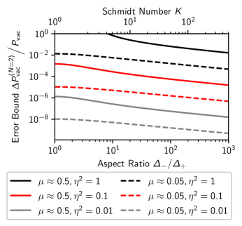
Figure 1: Relative error bound from LABEL:eq:FredholmDeterminantExpansion_RelativeError for the vacuum detection probabilities of a type-II SPDC state with a Gaussian JSA when truncating the logarithm series in the determinant expansion after order ${N=2}$. Different values of the total transmission $\eta^{2}$ and the mean number of generated photon pairs $\mu$ are considered.

II.4.2 Compression of the Determinant

A very common situation is that of some modes initially containing the vacuum state, e.g. due to beam splitters containing vacuum in one of their inputs. This can be used to effectively reduce the dimension of the covariance matrix and therefore significantly increase the computational performance when implementing the corresponding operations. Consider a system containing $M$ discrete modes, with ${M_{0}=M-M^{\prime}\geq 0}$ modes containing vacuum after all active transformations have been applied. Choosing the order of basis elements such that all vacuum modes are listed last, all transformations act according to

$$\bm{S}\left(\bm{\varGamma}\oplus\bm{0}_{2M_{0}\times 2M_{0}}\right)\bm{S}^{\dagger}=\bm{s}\bm{\varGamma}\bm{s}^{\dagger}\,,$$ (19)

where $\bm{\varGamma}$ is the ${2M^{\prime}\times 2M^{\prime}}$ renormalized covariance matrix describing only the modes initially not containing vacuum, $\bm{S}$ is the total ${2M\times 2M}$ transformation matrix, and $\bm{s}$ is a ${2M\times 2M^{\prime}}$ reduced transformation matrix containing only the first $2M^{\prime}$ columns of $\bm{S}$. Naively, the total transformation $\bm{S}$ is the composition of many subsequent $2M\times 2M$ transformations describing the components present in the setup. The total transformation $\bm{s}$ is obtained by multiplying ${2M\times 2M}$ matrices with ${2M\times 2M^{\prime}}$ matrices, resulting in a significant computational advantage for large $M_{0}$.

Furthermore, this allows us to apply the analogue of Sylvester’s determinant theorem for trace-class operators [Gohberg_2000] to extract the detection probabilities from the determinant of a smaller matrix:

$$\det\left(\mathds{1}_{2M}+\bm{P}\bm{s}\bm{\varGamma}\bm{s}^{\dagger}\bm{P}\right)=\det\left(\mathds{1}_{2M^{\prime}}+\bm{s}^{\dagger}\bm{P}\bm{s}\bm{\varGamma}\right)\,.$$ (20)

The term ${\bm{s}^{\dagger}\bm{P}\bm{s}}$ leads to the contributions of the different modes being added up before applying the determinant. For large matrices, the number of numerical operations to compute the determinant via the LU decomposition scales approximately with the third power of the matrix dimension [Trefethen_1997], thus the expected gain in performance amounts to a factor of $(M/M^{\prime})^{3}$. For example, the simulation of the QKD system we present in ref. Kleinpass_2024_partII requires ${M=12}$ discrete modes, however, initially only ${M^{\prime}=2}$ discrete modes (one for each party) contain a non-zero intensity. By using eq. 20, the size of the matrix for which the determinant is to be computed reduces by a factor of 6, resulting in $(M/M^{\prime})^{3}=216$.

The steps to compute the detection probabilities can be summarized as follows: First, construct the renormalized covariance after application of the last active transformation. Then, identify all remaining passive transformations describing the setup under consideration to compute the total transformation $\bm{s}$ analytically on the block-matrix level for the discrete modes only. Compute the analytic expression of ${\bm{s}^{\dagger}\bm{P}\bm{s}\bm{\varGamma}}$ depending on the modes over which a detection is performed, specified by $\bm{P}$. These steps can be simplified by using software for symbolic computations when many transformations or many discrete DOFs are involved. Finally, translate the products between the different blocks to integral transforms to obtain the detection probabilities in terms of the continuous DOFs. We demonstrate the procedure for two entanglement-based QKD systems in the second part of this series, ref. Kleinpass_2024_partII.

III Highly Entangled Biphoton States

In section III.1, the representation of biphoton states in the continuous covariance formalism is discussed. The series expansion of the renormalized covariance as well as an easily computable error bound are presented in section III.2, before explicitly examining the two lowest-order approximations in sections III.3 and LABEL:sec:Hermite_Approximations.

III.1 Covariance Representation of Biphoton States

For simplicity, photon pair generations in wave guide structures supporting only one spatial mode are considered. In the undepleted pump approximation, the state of the generated photon pairs after tracing out the pump signal reads [Yang_2008, Mauerer_2009, Quesada_2014, Thomas_2021]

$$\lvert\psi\rangle=\exp\left(\frac{C}{2}\!\int\!\!\dl\omega_{\mathrm{s}}\dl\omega_{\mathrm{i}}\psi(\omega_{\mathrm{s}},\omega_{\mathrm{i}})\hat{a}_{\nu}^{\dagger}(\omega_{\mathrm{s}})\hat{a}_{\rho}^{\dagger}(\omega_{\mathrm{i}})-\mathrm{H.c.}\!\right)\lvert 0\rangle\,,$$ (21)

where $\nu$ and $\rho$ label the polarization modes of the signal and idler photons and the coefficient $C$ incorporates all constant factors such as the intensity of the pump field and the strength of the non-linear interaction. The only non-vanishing commutator is ${[\hat{a}_{\nu}(\omega_{\mathrm{s}}),\hat{a}_{\rho}^{\dagger}(\omega_{\mathrm{i}})]=\delta_{\nu\rho}\delta(\omega_{\mathrm{s}}-\omega_{\mathrm{i}})}$.

A process is called type-0 or type-I (which we will summarize as type-0/I) if both generated photons share the same polarization, i.e. ${\nu=\rho}$ in eq. 21. Due to the waveguide supporting only one spatial mode, this leads to signal and idler being indistinguishable, i.e. featuring a symmetric JSA ${\psi(\omega_{\mathrm{s}},\omega_{\mathrm{i}})=\psi(\omega_{\mathrm{i}},\omega_{\mathrm{s}})}$. If they are polarized orthogonally to each other, i.e. $\nu\neq\rho$, the process is called type-II.

The joint spectral density (JSD) is the squared modulus of the JSA:

$$\Psi(\omega_{\mathrm{s}},\omega_{\mathrm{i}})=\lvert\psi(\omega_{\mathrm{s}},\omega_{\mathrm{i}})\rvert^{2}\,.$$ (22)

It describes the bivariate spectral probability density of the generated photons. As all constant factors are absorbed into $C$ in eq. 21, the JSD is normalized to

$$\int\dl\omega_{\mathrm{s}}\dl\omega_{\mathrm{i}}\Psi(\omega_{\mathrm{s}},\omega_{\mathrm{i}})=1\,.$$ (23)

The signal and idler spectral densities are given by the marginal distributions of the JSD:

rCl Ψ_s(ω_s) &= ∫Ψ(ω_s, ω_i) ω_i ,
Ψ_i(ω_i) = ∫Ψ(ω_s, ω_i) ω_s .

A common approach to simplify the biphoton state from eq. 21 for sufficiently small pump powers is to truncate the series expansion after the linear term [Keller_1997, Grice_1997, Law_2000, Mikhailova_2008, Lee_2014, Liu_2020, Phehlukwayo_2020, Dorfman_2021]

$$\lvert\psi\rangle\propto\left(\lvert 0\rangle+\frac{C}{2}\int\dl\omega_{\mathrm{s}}\dl\omega_{\mathrm{i}}\psi(\omega_{\mathrm{s}},\omega_{\mathrm{i}})\hat{a}_{\nu}^{\dagger}(\omega_{\mathrm{s}})\hat{a}_{\rho}^{\dagger}(\omega_{\mathrm{i}})\lvert 0\rangle\right)\,,$$ (25)

neglecting the possibility of multiple photon pairs being created simultaneously.

To include all orders of multi-pair events, the Gaussian state formalism may be employed. The quadratic unitary transformation in eq. 21 is re-written in the form of section II.1 to obtain c”c Z^(I) = C (0 ψ ψ†0 )  , & Z^(II) = C2 (0 0 0 ψ0 0 ψT00 ψ*0 0ψ†0 0 0 )  ,
for type-0/I and type-II processes, respectively, where $\bm{\psi}$ is the integral operator with kernel $\psi(\omega_{\mathrm{s}},\omega_{\mathrm{i}})$. The state is constructed by applying $\bm{Z}$ to the vacuum, such that, according to section II.1, the covariance is given by

$$\bm{\gamma}=\exp(2\bm{Z})\,.$$ (26)

The Schmidt decomposition [Law_2000, Lamata_2005, Mauerer_2009] of the JSA reads

$$\psi(\omega_{\mathrm{s}},\omega_{\mathrm{i}})=\sum_{j}\sqrt{\lambda_{j}}u_{j}(\omega_{\mathrm{s}})v_{j}^{*}(\omega_{\mathrm{i}})\,,$$ (27)

where the Schmidt modes $\{u_{j}(\omega)\}_{j}$ and $\{v_{j}(\omega)\}_{j}$ are two sets of orthonormal functions and the Schmidt coefficients $\{\sqrt{\lambda_{j}}\}_{j}$ are real, non-negative and enumerated in decreasing order ${\sqrt{\lambda_{j}}\geq\sqrt{\lambda_{j+1}}}$. The normalization in eq. 23 is represented by ${\sum_{j}\lambda_{j}=1}$.

The magnitude of the entanglement can be quantified by the Schmidt number ${K=1/\sum_{j}\lambda_{j}^{2}}$ [Fedorov_2006, Mikhailova_2008, Mauerer_2009, Horoshko_2018]. Its minimum value ${K=1}$ implies that ${\lambda_{1}=1}$ is the only non-zero Schmidt coefficient, corresponding to the JSD factorizing as ${\Psi(\omega_{\mathrm{s}},\omega_{\mathrm{i}})=\Psi_{\mathrm{s}}(\omega_{\mathrm{s}})\Psi_{\mathrm{i}}(\omega_{\mathrm{i}})}$, rendering the two photons independent from each other without any spectral entanglement between them. For a given number of non-zero Schmidt coefficients $J$, the Schmidt number takes its maximum value $K=J$ when all contributing coefficients are equal, i.e. ${\lambda_{j}=1/J}$ for ${j\leq J}$. Such a state is called maximally entangled.

In analogy to the singular value decomposition of a matrix [Trefethen_1997], the Schmidt decomposition of the Hilbert-Schmidt operator $\bm{\psi}$ with kernel $\psi(\omega_{\mathrm{s}},\omega_{\mathrm{i}})$ can be written compactly as ${\bm{\psi}=\bm{U}\bm{\Sigma}\bm{V}^{\dagger}}$, with the diagonal matrix $\bm{\Sigma}$ containing the singular values, that is, the Schmidt coefficients $\sqrt{\lambda_{j}}$. The columns of the unitary matrices $\bm{U}$ and $\bm{V}$ are the corresponding Schmidt modes of $\bm{\psi}$. This can be used to write the covariance in the form

rCl γ^(I) &= (U cosh(σ(I)) U†U sinh(σ(I)) V†V sinh(σ(I)) U†V cosh(σ(I)) V†)  ,
γ^(II) = (U cosh(σ(II)) U†U sinh(σ(II)) V†V sinh(σ(II)) U†V cosh(σ(II)) V†) ⨁c.c.  ,

for type-0/I and type-II processes, respectively, with the squeezing parameters c”c σ^(I) = 2C Σ  ,& σ^(II) = C Σ  . In the low-gain regime, where ${\cosh(\bm{\sigma})\approx\mathds{1}+\bm{\sigma}^{2}/2}$, the corresponding mean numbers of generated photons pairs $\mu$ are given by c”c μ^(I) ≈C^2/2  , & μ^(II) ≈C^2/4  . For type-II processes, the basis elements in eq. 28 have been reordered according to

$$\hat{\bm{\mathfrak{a}}}\to\big{(}\hat{a}(\omega),\hat{b}^{\dagger}(\omega),\hat{a}^{\dagger}(\omega),\hat{b}(\omega)\big{)}^{\mathrm{T}}\,,$$ (29)

where $\hat{a}(\omega)$ and $\hat{b}(\omega)$ correspond to the orthogonal polarization modes of signal and idler, respectively. LABEL:sec:Appendix_Eigenvalues_and_Generating_Functions shows how the eigenvalues of the renormalized covariance as well as the generating functions of the processes are obtained from the squeezing parameters.

III.2 Approximation of the Renormalized Covariance

For a large amount of spectral entanglement, the Schmidt decomposition of the JSA in eq. 28 becomes very challenging to evaluate in practice. Instead, the renormalized covariance can be approximated by truncating the series expansion of the exponential in eq. 26 at some sufficiently large order $N$:

$$\bm{\varGamma}_{N}\approx\sum_{n=1}^{N}\frac{(2\bm{Z})^{n}}{2n!}\,.$$ (30)

In LABEL:sec:Error_Bound_Renormalized_Covariance we show that the relative truncation error w.r.t. the trace norm is bounded by

$$\frac{\lVert\bm{\varGamma}-\bm{\varGamma}_{N}\rVert_{\mathrm{Tr}}}{\lVert\bm{\varGamma}\rVert_{\mathrm{Tr}}}\leq\left\{\begin{aligned} &\frac{\sum_{j=1}^{M}\left[\sinh(\sigma_{j})-\mathfrak{s}_{N}(\sigma_{j})\right]}{\sum_{j=1}^{M}\sinh(\sigma_{j})}&&\text{for $N$ even,}\\ &\frac{\sum_{j=1}^{M}\left[\cosh(\sigma_{j})-\mathfrak{c}_{N}(\sigma_{j})\right]}{\sum_{j=1}^{M}\sinh(\sigma_{j})}&&\text{for $N$ odd,}\end{aligned}\right.$$ (31)

for all $M\leq J$, where c”c c_N(x) = ∑_n{ 0 ≤2n ≤N } x2n(2n)!  , & s_N(x) = ∑_n{ 0 ≤2n+1 ≤N } x2n+1(2n+1)!  . are the contributions to the $\cosh(x)$ and $\sinh(x)$ series when truncating the expansion of $\exp(x)$ at order $N$, respectively. This means, that the relative error is bounded by the $M$ largest squeezing parameters, where equality holds for $M=J$.

The relative error in eq. 31 takes its maximum value in the non-entangled case, i.e. when all of the state’s energy is concentrated within one Schmidt mode. For an increasing amount of entanglement, more and more Schmidt modes become relevant and it becomes more and more expensive to perform an explicit Schmidt decomposition. At the same time, the relative error in eq. 31 decreases the more uniformly the energy is distributed amongst an increasing number of contributing Schmidt modes. Therefore, the more expensive it becomes to perform an explicit Schmidt decomposition, the faster the sum in eq. 31 converges and the easier it becomes to use this approximation.

In practice, to obtain a bound for the relative approximation error without performing a full Schmidt decomposition, it is sufficient to compute the $M$ largest squeezing parameters, which can be done by discretizing $\psi(\omega_{\mathrm{s}},\omega_{\mathrm{i}})$ and computing a truncated singular value decomposition of the resulting matrix [Golub_1965, Hochstenbach_2001, Halko_2011, Wu_2015]. Figure 2 shows the upper bound of the relative error for $M=1$, i.e. only using the largest squeezing parameter $\sigma_{1}$ and for different values of $\mu$ and $N$ over the aspect ratio ${\varDelta_{-}/\varDelta_{+}}$ of a 2D Gaussian JSA [Mauerer_2009].

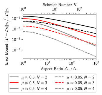
Figure 2: Relative error bound from eq. 31 for the $N$-th order approximation of the renormalized covariance of a type-II SPDC state with Gaussian JSA w.r.t. the trace norm. Different expansion orders $N$ and mean numbers of generated photon pairs $\mu$ are considered.

III.3 Bivariate Poisson Approximation

The lowest-order expansions of the covariance and determinant series provides further insights into the physical meaning of the different expansion orders. For the covariance, the approximation orders $N=0$ and $N=1$ in eq. 30 yield no contribution to the expected number of photons, such that the lowest non-trivial expansion order is given by $N=2$:

$$\bm{\varGamma}\approx\bm{Z}+\bm{Z}^{2}\,.$$ (32)

Similarly, as discussed in section II.4, at least a second order approximation of the logarithm is required to account for correlations. In the presence of any block-diagonal transformations, which we represent as frequency-dependent losses $\bm{\eta}$, i.e. ${\bm{\varGamma}\to\bm{\eta}\bm{\varGamma}\bm{\eta}}$, the resulting generating function reads

$$G^{(N=2)}(\bm{w})\approx\exp\left(-\frac{\operatorname{Tr}(\bm{W}\bm{\eta}\bm{\varGamma}\bm{\eta})}{2}+\frac{\lVert\bm{W}\bm{\eta}\bm{\varGamma}\bm{\eta}\rVert_{\mathrm{HS}}^{2}}{4}\right)\,.$$ (33)

Due to the anti-diagonal structure of $\bm{Z}$, only even orders of $\bm{Z}$ can contribute. Thus, the second term in eq. 33 is composed of two contributions after inserting eq. 32:

$$\lVert\bm{W}_{\bm{\eta}}\bm{\varGamma}\rVert_{\mathrm{HS}}^{2}=\underbrace{\lVert\bm{W}_{\bm{\eta}}\bm{Z}\rVert_{\mathrm{HS}}^{2}}_{\mathcal{O}(\psi^{2})}+\underbrace{\lVert\bm{W}_{\bm{\eta}}\bm{Z}^{2}\rVert_{\mathrm{HS}}^{2}}_{\mathcal{O}(\psi^{4})}\,.$$ (34)

For a large amount of spectral entanglement or a sufficiently small mean number of photon pairs, the $\mathcal{O}(\psi^{4})$ term can be neglected, such that

$$G^{(\mathrm{Poisson})}(\bm{w})=\exp\left[-\frac{1}{4}\operatorname{Tr}\left(\bm{Z}^{2}-\left[\left(\mathds{1}-\bm{W}_{\bm{\eta}}\right)\bm{Z}\right]^{2}\right)\right]\,,$$ (35)

where $\bm{W}_{\bm{\eta}}=\bm{\eta}\bm{W}\bm{\eta}$. This can be rewritten according to

$$G^{(\mathrm{Poisson})}(\bm{w})=\mathrm{e}^{-\mu\left(w_{\mathrm{s}}p_{\mathrm{s}}(I_{\mathrm{s}})+w_{\mathrm{i}}p_{\mathrm{i}}(I_{\mathrm{i}})-w_{\mathrm{s}}w_{\mathrm{i}}p_{\mathrm{s},\mathrm{i}}(I_{\mathrm{s}}\cap I_{\mathrm{i}})\right)}\,,$$ (36)

where $\mu$ is given by eq. 28.
For type-II processes,

rCl p_s(I_s) &= Tr( W_η ψ ψ^†) = ∫_I_s ω