BIGCity: A Universal Spatiotemporal Model for Unified Trajectory and Traffic State Data Analysis

Abstract

Spatiotemporal (ST) data analysis is a critical area of research in data engineering. Typical dynamic ST data includes trajectory data (representing individual-level mobility) and traffic state data (representing population-level mobility). Traditional studies often treat trajectory and traffic state data as distinct, independent modalities, each tailored to specific tasks within a single modality. However, real-world applications, such as navigation apps, require joint analysis of trajectory and traffic state data. Treating these data types as two separate domains can lead to suboptimal model performance. Although recent advances in ST data pre-training and ST foundation models aim to develop universal models for ST data analysis, most existing models are “multi-task, solo-data modality” (MTSM), meaning they can handle multiple tasks within either trajectory data or traffic state data, but not both simultaneously.

To address this gap, this paper introduces BIGCity, the first multi-task, multi-data modality (MTMD) model for ST data analysis. The model targets two key challenges in designing an MTMD ST model: (1) unifying the representations of different ST data modalities, and (2) unifying heterogeneous ST analysis tasks. To overcome the first challenge, BIGCity introduces a novel ST-unit that represents both trajectories and traffic states in a unified format. Additionally, for the second challenge, BIGCity adopts a tunable large model with ST task-oriented prompt, enabling it to perform a range of heterogeneous tasks without the need for fine-tuning. Extensive experiments on real-world datasets demonstrate that BIGCity achieves state-of-the-art performance across 8 tasks, outperforming 18 baselines. To the best of our knowledge, BIGCity is the first model capable of handling both trajectories and traffic states for diverse heterogeneous tasks. Our code are available at https://github.com/bigscity/BIGCity.

I Introduction

Spatiotemporal (ST) data analysis has been a cornerstone of research in data engineering, with models such as trajectory analysis and traffic state prediction playing critical roles in various domains. These models are integral to the development of intelligent transportation systems (ITS) [1, 2], smart cities [3, 4, 5, 6, 7, 8], and location-based service (LBS) applications [9], enabling advanced solutions for urban mobility, infrastructure planning, and personalized services.

From a data perspective, ST data analysis models are categorized into two types based on the targeted data: individual-level models for trajectory data and population-level models for traffic state data. Individual-level trajectory models, such as next-hop prediction [10, 11, 12, 13], trajectory-user linkage [14, 15], and trajectory traffic pattern classification [16], process mobility trajectories of individuals on road networks or among POIs to uncover patterns in individual human mobility. Population-level traffic state models, including traffic state prediction [17, 18], traffic state imputation [19, 20] and etc, analyze time series data on traffic metrics like speed, density, and flow volumes. These models aim to capture spatiotemporal correlations at a population level, reflecting crowd behaviors in transportation systems, such as urban road networks.

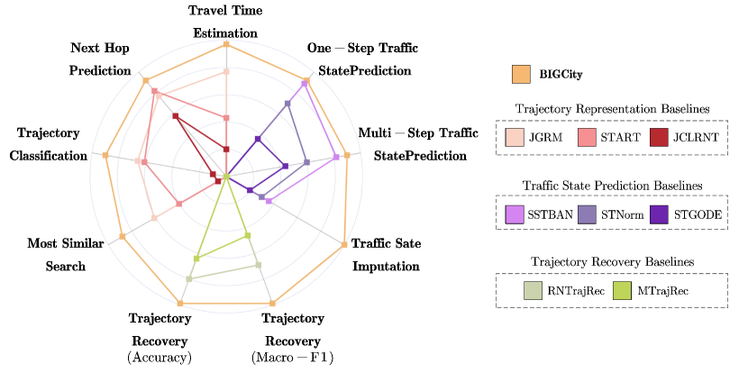
Figure 1: Performance Radarchart of BIGCity on Various Tasks.

In the literature, current ST data analysis methods are often narrowly tailored to specific types of data, focusing either on trajectories or traffic states. Most studies treat trajectories and traffic states as entirely distinct data modalities, designing task-specific models for one modality (sole task in sole data modality (STSD)). A model designed for trajectory next-hop prediction cannot be applied to tasks like trajectory-user linkage, let alone traffic state prediction. While some ST data pre-training models, such as trajectory or time-series representation learning models, can generate universal representation vectors for multiple downstream tasks [16, 21], they remain limited to handling a single data modality, either trajectories or traffic states (multiple tasks in sole data modality (MTSD)).

However, individual-level mobility behaviors and population-level traffic states are intrinsically interconnected. Macro-level traffic states are aggregated from micro-level individual trajectories, while population traffic states influence individual mobility patterns. Many ITS and LBS applications require analyzing trajectory and traffic state data jointly. For example, car-hailing platforms need to predict the location of a taxi while considering traffic speed predictions. Treating trajectories and traffic states as separate domains in such scenarios can lead to suboptimal model performance.

In recent years, significant efforts have been made to develop universal foundation models for ST data. Models such as UniST [22], UrbanGPT [23], and OpenCity [24] focus on unified frameworks for traffic state analysis across cities, while UniTraj [25] and TrajCogn [26] aim to handle diverse trajectory analysis tasks using a single model. CityFM [27] generates universal representations for static geographical units. Despite their success in supporting multiple tasks [25], cross-dataset knowledge transfer [22], and few-/zero-shot data analysis [24], these models remain limited to MTSD. A truly versatile model capable of handling diverse ST data analysis tasks across both trajectories and traffic states (multiple tasks in multiple data modalities (MTMD)) is still lacking.

Outside the field of ST data analysis, versatile and universal foundation models capable of processing heterogeneous data with a single framework have become widespread in domains such as text processing and image processing [28]. Notable examples include the success of large language models (LLMs) like [29, 30] in natural language processing and visual-language multimodal data analysis [31]. Despite the achievements of versatile models in these fields, developing a MTMD model for ST data remains constrained by several unique challenges, as outlined below.

(1) Challenges in unified representations of ST data: In NLP, all text data can be uniformly represented as sequences of characters (unified units), and in CV, images are uniformly represented as matrices or tensors of pixels (unified units). However, in ST data analysis, trajectories are modeled as sequences of geographical units (e.g., road segments or POIs), while traffic states are represented as graphs with dynamic signals (e.g., traffic speed over road networks). The differing basic units make developing a unified representation framework for the two data modalities a significant challenge.

(2) Challenges in unifying heterogeneous ST analysis tasks: In NLP, diverse tasks can be unified as next-word generation, enabling a single model to handle various tasks efficiently. However, in ST data analysis, tasks are highly heterogeneous, with even identical inputs requiring different outputs. For instance, given the same trajectory inputs, travel time estimation outputs continuous timestamps, while user-trajectory linkage outputs discrete user IDs. Unifying such heterogeneous tasks within a single data processing and model training framework remains a significant challenge.

To address these challenges, we propose a Bi-modality unIfied General model for ST data analysis in road network-based City scenarios (BIGCity). BIGCity focuses on road networks as the foundational scenario for ST data analysis. To tackle the challenge of unified data representation, BIGCity introduces ST-units (see Sec. IV-A), enabling the expression of ST data from both trajectories and traffic state series in a unified format, i.e., a sequence of ST-units. These ST-units are further embedded into token sequences via a neural network-based Spatiotemporal Tokenizer (see Sec. IV-B). To address the challenge of task heterogeneity, we propose a Universal ST Model with Task-oriented Prompt (VMTP) (see Sec. V), which employs novel Task-oriented Prompts to guide an LLM-based Tunable Model for executing diverse ST analysis tasks. Additionally, we design a two-stage training strategy (see Sec. VI), combining self-supervised masked reconstruction and task-oriented prompt tuning, to train the model on heterogeneous ST data for multiple tasks. Extensive experiments on three real-world datasets involving both trajectory and traffic state data demonstrate that BIGCity outperforms 18 baselines across 8 tasks, highlighting its superior performance and versatility.

Here, we summarize our key contributions:

• To the best of our knowledge, BIGCity is the first model capable of handling multiple types of data analysis tasks for both trajectory and traffic state data, making it the first MTMD ST data analysis model.

• We propose a unified ST data representation method, i.e., ST-units and ST tokens, along with a novel universal model with task-oriented prompts to unify heterogeneous ST analysis tasks. These methods address the challenges of constructing unified representations for distinct ST data modalities and adapting to heterogeneous ST analysis tasks.

• Our model achieves state-of-the-art performance on 3 real-world datasets, surpassing 18 baselines across 8 tasks. To our knowledge, BIGCity is the first model to achieve SOTA performance over such a wide range of baselines and tasks.

II Related Works

II-A Spatiotemporal Data Analysis Models (STSD Models)

STSD models are trained to capture specific temporal and spatial dependencies, addressing a specific task such as traffic state prediction [32, 33, 34, 35, 36], trajectory prediction [37, 38, 39, 40], trajectory classification [41, 42]. As a result, the model architectures vary with task type. For temporal dependency modeling, current models employ recurrent neural networks [43, 44], temporal convolutional networks [45, 46], or attention mechanism [47]. For spatial dependency modeling, they utilize graph neural networks [48, 49, 17] or attention mechanism over graphs [2]. Beyond the above models, physics-guided deep learning approaches have recently emerged, providing deeper theoretical insights into spatiotemporal data analysis (STSD) [5, 50, 51, 52, 46]. These models provide stronger interpretable ability, addressing limitations of deep models.

Summary: Despite their success, most of the existing methods are specifically designed for a single data modality and specific tasks, i.e., STSM. They requires separate models to handle trajectory and traffic state data. In contrast, BIGCity can handle trajectories and traffic states within a single model.

II-B Spatiotemporal Representation learning (MTSD Models)

Self-supervised pre-training representation learning is crucial for multi-task ST data analysis. Existing trajectory models [3, 15, 53, 54, 55, 56, 57, 58, 59] employ sequential models with self-supervised tasks, while traffic state models [60, 61, 62, 32, 43, 17, 45, 63, 64, 65] leverage graph neural networks (GNNs) [66] to capture spatiotemporal dependencies for predicting future traffic states. Recent models have focused on integrating more comprehensive ST features. For example, trajectory models like TremBR [14] and START [15] account for temporal periodicity, while traffic state models such as T-wave [67], TrajNet [68], and TrGNN [69] capture multi-hop spatial dependencies along trajectories. Beyond these models, VecCity [70] proposed a comprehensive ST models library, where each map entity is represented as a vector. Furthermore, recent works [27, 71] have introduced text representations using large language models.

Summary: While existing models often overlap in the trajectory and traffic state domains, such as incorporating traffic state into trajectory representations, they are typically focused on a single data modality, i.e., MTSD models. Furthermore, these models require fine-tuning for different downstream tasks, resulting in “semi-multi-task” functionality. While BIGCity handles various tasks without task-specific fine-tuning.

II-C Universal Spatiotemporal Models (ST Foundation Models)

The target of this kind of model is to design a universal foundation model for ST data analysis, similar to LLMs for NLP. There are two main research directions for spatiotemporal universal models: 1) Cross-Dataset Universal Models: These models aim to generalize across different datasets (e.g., datasets from various cities), enabling rapid adaptation to new datasets through few-shot or zero-shot learning [72, 73, 23, 74, 22, 75, 76, 77, 78, 24, 79] for traffic states or trajectory analysis. For example, approaches [80, 81] treat LLMs as spatio-temporal encoders, training them for traffic prediction over cross-data sets. UniST [22] introduced spatiotemporal prompt learning, using statistical features of the dataset as prompts for the prediction of cross-dataset traffic. 2) Universal Models for Heterogeneous Tasks: These models focus on multi-task capabilities, with one strategy involving training from scratch on large datasets [82] to adapting heterogeneous with the same data modalities. Recent works [83, 84, 85, 86, 87, 88, 26] exploit LLMs’ multi-task capabilities by converting trajectory data into textual format. Other works leverage LLMs’ linguistic abilities to improve model generalization via in-context learning [23] and provide interpretable outputs [89]. Some efforts explore LLMs as spatiotemporal agents, bridging LLMs with tools to perform traffic-related queries and reasoning based on human instructions [90].

Summary: Many of these universal ST models leverage LLM technologies for task versatility and cross-dataset knowledge transfer. These models effectively address the “semi-multi-task” limitation of ST representation learning by eliminating the need for fine-tuning in downstream applications. However, most of these models are limited to handling either trajectory or traffic state data, but not both. In contrast, BIGCity not only addresses the “semi-multi-task” issue by offering task versatility but also handles both trajectory and traffic state data, achieving true data modality versatility.

III Preliminaries

Our model is designed for road network-based urban traffic scenarios, where the city is represented as a road network and ST data are generated from individuals’ movements. These scenarios are common in many widely used ST datasets. This section outlines the basic spatial and temporal components of such scenarios, defining the two types of dynamic spatiotemporal data: trajectories and traffic states.

III-A Basic Spatial and Temporal Elements

The basic spatial elements in the scenario are road segments.

Definition 1 (Road Segment).

Consider a city map with $I$ road segments, denoted as $r_{i}$ for the $i$-th segment. The set of segments is $\mathcal{R}=\{r_{1},\cdots,r_{i},\cdots,r_{I}\}$. Each segment $r_{i}$ is associated with a static feature vector $\bm{e}_{i}^{(s)}\in\mathbb{R}^{D_{r}}$, describing attributes such as road ID, type, length, lane count, in-degree, out-degree, speed limit, and other relevant characteristics.

All road segments collectively form a road network.

Definition 2 (Road Network).

A road network is a directed graph denoted as $\mathcal{G}=\{\mathcal{R},\mathcal{A},\bm{E}^{(s)}\}$, where $\mathcal{R}$ is the set of vertices corresponding to road segments. $\mathcal{A}\in\mathbb{R}^{|\mathcal{R}|\times|\mathcal{R}|}$ is the binary adjacency matrix indicating connectivity between road segments. $\bm{E}^{(s)}=\big{(}\bm{e}_{1}^{(s)},\cdots,\bm{e}_{n}^{(s)},\cdots,\bm{e}_{N}^{(s)}\big{)}$ represents the static feature vectors for all road segments.

The basic temporal elements are conceptualized in two forms: discrete time slice and continuous timestamp.

Definition 3 (Time Slice).

A time slice is a fixed-length interval partitioning the timeline, indexed as $\{1,\cdots,t,\cdots,T\}$. For the $t$-th time slice, a feature vector $\bm{\iota}_{t}\in\mathbb{R}^{D_{t}}$ is defined to describe its attributes, such as the slice’s start time, its index within a day, the day index within a week, and so on.

Definition 4 (Timestamp).

A timestamp represents an instantaneous UTC time, denoted as $\tau$. For a given timestamp $\tau$, a feature vector $\bm{\iota}_{\tau}\in\mathbb{R}^{D_{\tau}}$ describes its attributes, including its absolute timeand the features of the time slice it belongs to.

In BIGCity, both discrete and continuous temporal elements coexist. For a time slice $t$, its start time is represented by the timestamp $\tau_{t}$, and for a timestamp $\tau$, the corresponding time slice is denoted as $t_{\tau}$.

III-B Dynamic Spatiotemporal Data

Based on the above elements, dynamic ST data can be categorized into two types: individual-level trajectories and population-level traffic states. Trajectories capture individual mobility behaviors, defined as follows:

Definition 5 (Trajectory).

A trajectory is a time-ordered sequence of road segments with associated timestamps, defined as ${tr}=\big{(}(r_{tr_{1}},\tau_{tr_{1}}),$ $\dots,$ $(r_{tr_{l}},\tau_{tr_{l}}),$ $\dots,$ $(r_{tr_{L}},\tau_{tr_{L}})\big{)}$, where $(r_{tr_{l}},\tau_{tr_{l}})$ is the $l$-th sample in the trajectory. Here, $r_{tr_{l}}\in\mathcal{R}$ is the road segment, and $\tau_{tr_{l}}$ is the corresponding timestamp. The trajectory can also be expressed as ${tr}=\big{(}(\bm{e}^{(s)}_{tr_{1}},\tau_{tr_{1}}),$ $\dots,$ $(\bm{e}^{(s)}_{tr_{l}},\tau_{tr_{l}}),$ $\dots,$ $(\bm{e}^{(s)}_{tr_{L}},\tau_{tr_{L}})\big{)}$, where $\bm{e}^{(s)}_{tr_{l}}$ denotes the static feature of road segment $r_{tr_{l}}$.

Definition 6 (Traffic State).

For a given time slice $t$, the traffic state of the road segment $r_{i}$ is represented as a vector $\bm{e}^{(d)}_{i,t}\in\mathbb{R}^{D_{d}}$, contains the dynamic characteristics of $r_{i}$, such as average speed, traffic entry and exit. $D_{d}$ is the number of traffic state channels. The traffic state series for $r_{i}$ is ${ts}_{i}=\big{(}\bm{e}^{(d)}_{i,1},$ $\dots,$ $\bm{e}^{(d)}_{i,t},$ $\dots,$ $\bm{e}^{(d)}_{i,T}\big{)}$. Using the start time of each time slice as its timestamp, we have ${ts}_{i}=\big{(}(\bm{e}^{(d)}_{i,1},\tau_{1}),$ $\dots,$ $(\bm{e}^{(d)}_{i,t},\tau_{t}),$ $\dots,$ $(\bm{e}^{(d)}_{i,T},\tau_{T})\big{)}$, where $\tau_{t}$ is the timestamp of time slice $t$.

According to Def. 5 and 6, both trajectories and traffic states are sequences of the basic spatial and temporal elements.

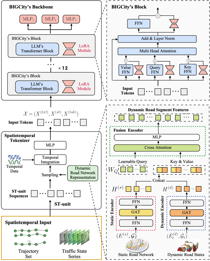
Figure 2: The model architecture of BIGCity.

III-C Motivation of BIGCity

Trajectories and traffic states represent human mobility patterns at different levels: individual-level and population-level, respectively. Although typically treated as distinct, heterogeneous data modalities, these two types of data are inherently interconnected. According to Def. 5 and Def. 6, both trajectories and traffic states share similar structural formats.

• For a trajectory, a sample corresponds to the road segment where an individual is located at a given sampling time, and the location is associated with a corresponding traffic state.

• For a traffic state series, a sample represents the dynamic traffic state of a road segment at a given sampling time.

Thus, the triple $(\mathrm{segment},\mathrm{traffic~{}state},\mathrm{sampling~{}time})$, i.e., “a road segment with its traffic state sampled at a specific time”, can be seen as the basic unit of ST data, analogous to words in NLP or pixels in image data. This insight suggests a viable opportunity to develop a versatile MTMD model that simultaneously handles both trajectories and traffic states.

Based on this idea, we propose BIGCity as to achieve MTMD ST modeling. Figure 2 illustrates the framework, which consists of two core components: $i$) a Unified ST Tokenizer to address heterogeneous data representation (Sec. IV), and $ii$) a Versatile ST Model with Task-oriented Prompt to handle distinct ST tasks (Sec. V).

IV Unified Representations for ST Data

In this section, we address Challenge 1: the unification of spatiotemporal data representations for MTMD model design. We first define spatiotemporal units (ST-units) as a unified representation for both trajectories and traffic states. Then, we introduce the Spatiotemporal Tokenizer to encode these ST-units into input tokens (ST tokens) for BIGCity.

IV-A Basic Spatiotemporal Units

Building on the motivation in Sec. III-C, we define the triple $(\mathrm{segment},\mathrm{traffic~{}state},\mathrm{sampling~{}time})$ as the basic spatiotemporal unit (ST-unit) for both trajectory and traffic state data. Formally, for a road segment $r_{i}$ and a timestamp $\tau$, an ST-unit is expressed as:

$$\small\bm{U}_{i,\tau}=\left(\bm{e}^{(s)}_{i},\bm{e}^{(d)}_{i,t_{\tau}},\bm{\iota}_{\tau}\right),$$ (1)

where $\bm{e}^{(s)}_{i}$ represents the static features of segment $r_{i}$, $\bm{\iota}_{\tau}$ is the timestamp feature for $\tau$, and $\bm{e}^{(d)}_{i,t_{\tau}}$ represents the dynamic traffic state of segment $r_{i}$ at the time slice containing $\tau$.

Using the ST-unit in Eq. (1), we redefine traffic states and trajectories in a unified format as sequences of ST-units.

Definition 7 (ST-unit-based Traffic State).

For a road segment $r_{i}$, its traffic state series is redefined as:

$$\small\mathbf{\mathcal{U}}_{i}=\Big{(}\bm{U}_{i,\tau_{1}},\cdots,\bm{U}_{i,\tau_{t}},\cdots,\bm{U}_{i,\tau_{T}}\Big{)},$$ (2)

where $\bm{U}_{i,\tau_{t}}=\big{(}\bm{e}^{(s)}_{i},\bm{e}^{(d)}_{i,t},\bm{\iota}_{\tau_{t}}\big{)}$. Here, $\bm{\iota}_{\tau_{t}}$ represents the features of the timestamp $\tau_{t}$, and $\tau_{t}$ is the start time of time slice $t$.

Definition 8 (ST-unit-based Trajectory).

Given a trajectory $tr$ of length $L$, its ST-unit-based representation is defined as:

$$\small\mathbf{\mathcal{U}}_{{tr}}=\Big{(}\bm{U}_{{tr}_{1}},\cdots,\bm{U}_{{tr}_{l}},\cdots,\bm{U}_{{tr}_{L}}\Big{)},$$ (3)

where $\bm{U}_{{tr}_{l}}=\big{(}\bm{e}^{(s)}_{tr_{l}},\bm{e}^{(d)}_{tr_{l},t_{tr_{l}}},\bm{\iota}_{\tau_{tr_{l}}}\big{)}$ denotes the ST-unit for the $l$-th sample. Here, $\bm{e}^{(s)}_{tr_{l}}$ represents the static features of road segment $tr_{l}$, $\bm{e}^{(d)}_{tr_{l},t_{tr_{l}}}$ the dynamic features at time slice $t_{tr_{l}}$, and $\bm{\iota}_{\tau_{tr_{l}}}$ the timestamp feature of $\tau_{tr_{l}}$.

In certain datasets, road segments may lack dynamic features. In such cases, we set $\bm{e}^{(d)}_{tr_{l},\tau_{tr_{l}}}=\mathrm{NULL}$.

Remark: In Eq. (3) and Eq. (2), both individual-level trajectories and population-level traffic states, despite their heterogeneous modalities, are represented in a unified format – sequences of ST-units. This unification resolves the challenge of heterogeneous data representation, enabling the design of a model capable of analyzing multiple ST data modalities.

IV-B Spatiotemporal Tokenizer

This subsection presents the spatiotemporal (ST) tokenizer, which converts ST-units into token vectors (ST-tokens). Specifically, it first generates dynamic road network representations as ST feature library, and then samples specific features for input data according to ST-units. The tokenizer comprises four modules: a static feature encoder, a dynamic feature encoder, a fusion encoder, and a temporal integration module.

Static Feature Encoder. This module encodes the static features $\bm{e}^{(s)}_{i}$ of an ST-unit into a representation vector. To capture the spatial and topological relationships among road segments, the encoder employs a graph attention network (GAT) [91], generating segment representations based on the road network $\mathcal{G}=\{\mathcal{R},\mathcal{A},\bm{E}^{(s)}\}$ defined in Def. 2. Specifically, for the static feature matrix $\bm{E}^{(s)}=\big{(}\bm{e}^{(s)}_{1},\dots,\bm{e}^{(s)}_{N}\big{)}$, the encoder outputs a representation matrix $\bm{H}^{(s)}$ as follows:

$$\small\bm{H}^{(s)}=\mathrm{FFN}\left(\mathrm{GAT}_{s}\big{(}\bm{E}^{(s)},\mathcal{G}\big{)}\right),$$ (4)

where $\mathrm{GAT}_{s}(\cdot,\cdot)$ is the GAT model and $\mathrm{FFN}(\cdot)$ a feed-forward network for dimensional transformation. The result is $\bm{H}^{(s)}=\big{(}\bm{h}^{(s)}_{1},\dots,\bm{h}^{(s)}_{I}\big{)}$, with $\bm{h}^{(s)}_{i}\in\mathbb{R}^{D_{h}}$ as the static representation for road segment $r_{i}$.

Dynamic Feature Encoder. This module encodes the dynamic features $\bm{e}^{(d)}_{i,\tau}$ of an ST-unit into a representation vector. To capture temporal dependencies, historical features are incorporated from a time window of length $T^{\prime}$. For time slice $t$, the window is defined as $W=(t-T^{\prime},\cdots,t-1,t)$, and the concatenated historical features for segment $r_{i}$ are $\tilde{\bm{e}}^{(d)}_{i,t}=\left(\bm{e}^{(d)}_{i,t-T^{\prime}}\big{\|}\cdots\big{\|}\bm{e}^{(d)}_{i,t}\right)$, where $\|$ denotes concatenation. The integrated historical dynamic feature matrix is $\tilde{\bm{E}}^{(d)}_{t}=\big{(}\tilde{\bm{e}}^{(d)}_{1,t},\cdots,\tilde{\bm{e}}^{(d)}_{I,t}\big{)}$. By replacing the static feature matrix in the road network with $\tilde{\bm{E}}^{(d)}_{t}$, a dynamic road network $\tilde{\mathcal{G}}_{t}=\{\mathcal{R},\mathcal{A},\tilde{\bm{E}}^{(d)}_{t}\}$ is constructed. The dynamic feature encoder uses a GAT to encode $\tilde{\mathcal{G}}_{t}$ as:

$$\small\bm{H}^{(d)}_{t}=\mathrm{FFN}\Big{(}\mathrm{GAT}_{d}\big{(}\tilde{\bm{E}}^{(d)}_{t},\tilde{\mathcal{G}}_{t}\big{)}\Big{)},$$ (5)

where the result $\bm{H}^{(d)}_{t}=\big{(}\bm{h}^{(d)}_{1,t},\cdots,\bm{h}^{(d)}_{I,t}\big{)}$ represents the dynamic representation of segment $r_{i}$ at time slice $t$.

Fusion Encoder. This module fuses static and dynamic representations of road segments to generate comprehensive spatial representations. The concatenated representation for segment $r_{i}$ at time slice $t$ is $\bm{h}_{i,t}=\big{(}\bm{h}^{(s)}_{i}\|\bm{h}^{(d)}_{i,t}\big{)}$. A cross-attention mechanism is employed to capture long-range dependencies among these representations. Specifically, for segments $r_{i}$ and $r_{j}$, their relationship is computed as:

$$\small\alpha_{ij}=\Big{(}{\bm{q}_{i}^{\top}\bm{h}_{j,t}}\Big{)}\Big{/}{\sqrt{2D_{h}}},$$ (6)

where $\bm{W}_{Q}\in\mathbb{R}^{I\times D_{h}}$ is a learnable query matrix, and $q_{i}$ is the $i$-th vector The fused spatial representation for $r_{i}$ at time slice $t$ is then:

$$\small\bm{s}_{i,t}=\sum_{j=1}^{I}\mathrm{ATT}_{ij}\cdot\bm{h}_{j,t},\;\;\;\mathrm{where}\;\;\;\mathrm{ATT}_{ij}={\alpha_{ij}}\Big{/}{\sum_{j=1}^{I}\alpha_{ij}}.$$ (7)

Unlike the GAT used in the static and dynamic encoders, which only capture correlations between directly connected segments, the cross-attention mechanism enables long-range dependencies across all segments.

Temporal Integration & ST Tokens. This module integrates the timestamp and its features with the spatial representation to generate an ST token. Specifically, for a ST-unit $\bm{U}_{i,\tau}=\big{(}\bm{e}^{(s)}_{i},\bm{e}^{(d)}_{i,t_{\tau}},\bm{\iota}_{\tau}\big{)}$, the static and dynamic features $\bm{e}^{(s)}_{i}$ and $\bm{e}^{(d)}_{i,t_{\tau}}$ are encoded into a spatial representation $\bm{s}_{i,t_{\tau}}$. An MLP then combines $\bm{s}_{i,t_{\tau}}$ with the timestamp feature $\bm{\iota}_{\tau}$ and the time interval $\delta_{\tau}$ between adjacent ST-units to generate the ST token:

$$\small\bm{x}_{i,\tau}=\mathrm{MLP}\Big{(}\;\bm{s}_{i,t_{\tau}}\big{\|}\bm{\iota}_{\tau}\big{\|}\delta_{\tau}\Big{)},$$ (8)

where $\delta_{\tau}$ is the time interval between consecutive ST-units in a sequence. For a sequence of ST-units $(\bm{U}_{1},\cdots,\bm{U}_{l},\cdots,\bm{U}_{L})$ corresponding to a trajectory or traffic state series, the interval is $\delta_{\tau_{l}}=\tau_{l}-\tau_{l-1}$. Including $\delta_{\tau_{l}}$ helps the model handle non-uniformly spaced ST-unit sequences, which is crucial for real-world trajectory data with irregular sampling intervals. The resulting vector $\bm{x}_{i,\tau}$ is the ST Token for ST-unit $\bm{U}_{i,\tau}$.

Remark: The ST tokenizer converts a sequence of ST-units, representing either a trajectory or a traffic state series, into an ST-token sequence. Specifically, it transforms the trajectory $\mathcal{U}_{\mathrm{tr}}$ (Eq. (3)) into $\bm{X}_{tr}=\big{(}\bm{x}_{tr_{1}},\cdots,\bm{x}_{tr_{L}}\big{)}$, and the traffic state series $\mathcal{U}_{i}$ (Eq. (2)) into $\bm{X}_{i}=\big{(}\bm{x}_{i,\tau_{1}},\cdots,\bm{x}_{i,\tau_{T}}\big{)}$. These ST-token sequences serve as unified inputs for the BIGCity model, allowing it to process heterogeneous ST data across modalities. Thus, both individual-level trajectories and population-level traffic states are represented in a unified form, enabling seamless processing by a single model.

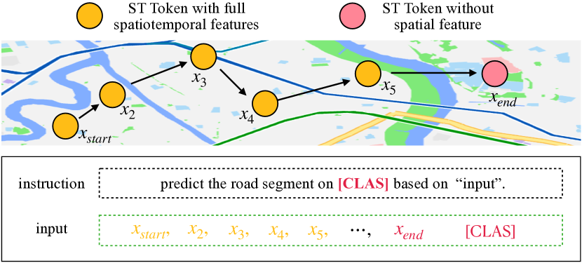
(a) Template of Next Hop Prediction

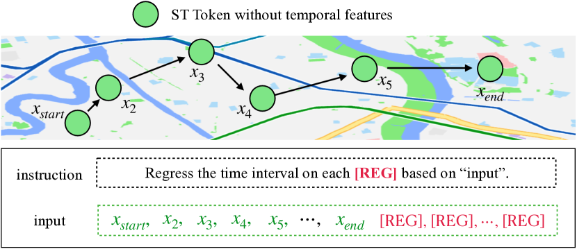
(b) Template of TTE Task

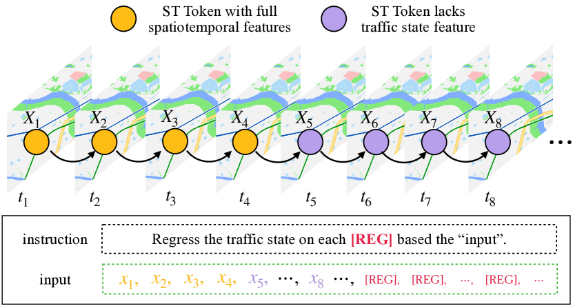
(c) Template of Traffic State Prediction

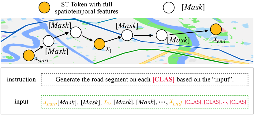
(d) Template of Trajectory Recovery

Figure 3: The templates for Task-oriented Prompts with different tasks.

V Versatile Model with Task Oriented Prompt

This section introduces a method to address the challenge of adapting to diverse ST analysis tasks (Challenge 2) for designing an MTMD model. A key difficulty for this challenge lies in informing the model about the specific task it should perform. Even with identical data inputs, different tasks require distinct types of outputs. For instance, given the same trajectory inputs, the travel time estimation task outputs continuous arrival time predictions, while the user-trajectory linkage task outputs discrete user ID.

Drawing inspiration from the prompt mechanism in LLMs, we propose a Versatile Model with Task-oriented Prompts (VMTP) to address this difficulty. VMTP employs textual instructions as prompts to guide the model on the desired task and utilizes a tunable LLM with ST tokens as inputs to perform specific ST data analysis tasks. The model consists of three modules: Task-oriented Prompts (input module), LLM-based Backbone Model (data-processing module), and General-task Heads (output module).

V-A Task-oriented Prompts

The input to our model is a task-oriented prompt that combines the ST token sequences generated by the ST tokenizer in Sec. IV-B with textual instructions specifying the type of task to be performed.

Prompt Contents. The task-oriented prompt consists of three components:

• Textual Instructions. This part of the prompt is a textual description of the data analysis task to be executed. For example, the instruction “Where is the next hop position of the input trajectory?” informs the model to perform a next hop prediction task. We use the tokenizer of the backbone LLM (see Sec. V-B) to converts the instructions into a sequence of Text Tokens, denoted as $\bm{X}^{(\mathrm{txt})}$.

• Input Data. This part of the prompt provides the spatiotemporal data to be analyzed, such as a traffic state series or a trajectory, formatted as ST-unit sequences according to Eq. (2) or Eq. (3). The ST tokenizer, as described in Sec. IV-B, converts these sequences into a series of ST Tokens, denoted as $\bm{X}^{(\mathrm{st})}$.

• Task Placeholders. This part of the prompt provides a format guide for the task outputs. Two types of placeholders are used: the classification placeholder, denoted as $[\mathrm{CLAS}]$, and the regression placeholder, denoted as $[\mathrm{REG}]$. These placeholders represent the expected output structure of the ST data analysis task. We use two learnable token vectors, $\bm{x}^{(\mathrm{clas})}$ and $\bm{x}^{(\mathrm{reg})}$, to corresponding to the two types of placeholders. The sequence of learnable token vectors is named as Task Tokens and denoted as $\bm{X}^{(\mathrm{tsk})}$.

The complete inputs to the VMTP model is a combined sequence consisting of the text tokens $\bm{X}^{(\mathrm{txt})}$, the ST tokens $\bm{X}^{(\mathrm{st})}$, and the task tokens $\bm{X}^{(\mathrm{tsk})}$, named as input prompt tokens, represented as:

$$\small\bm{\mathcal{X}}=\left(\bm{X}^{(\mathrm{txt})},\bm{X}^{(\mathrm{st})},\bm{X}^{(\mathrm{tsk})}\right).$$ (9)

Prompt Templates. As illustrated in the examples in Fig. 3, we use a template to organize the instructions, input data, and task placeholders of task-oriented prompts into a unified structure for various tasks.

The first part of the template is the instruction. For each task, we start by using a language model, specifically ChatGPT, to understand the task’s function. Then, the language model generates a set of candidate instructions describing the task. For example, for the travel time estimation task, candidate instructions might include: “Give me the estimated time of arrival for the input trajectory” or “When will I walk to the ending position in this trajectory?”. Finally, we evaluate these candidates and select the most effective instruction based on testing. This selected instruction is then used as a fixed component in the prompt template.

The second and third parts of the template are the input data and task placeholders. These components vary slightly depending on the type of task:

• For classification tasks, such as trajectory next hop prediction and user-trajectory linkage, the input data consists of a sequence of ST tokens corresponding to a trajectory to be classified. The task placeholder is a classification placeholder $[\mathrm{CLAS}]$ (see Fig. 3(a)).

• For regression tasks, such as trajectory travel time estimation (TTE) and traffic state prediction, the input data is a sequence of ST tokens corresponding to a trajectory or traffic state series. The task placeholder is a sequence of regression placeholder$[\mathrm{REG}]$ (see Fig. 3(b) and Fig. 3(c)).

• For generation tasks, such as trajectory recovery, the input consists of a sequence of ST tokens with $[\mathrm{MASK}]$ inserted at the positions to be generated. In recovery, $[\mathrm{MASK}]$ are placed between adjacent samples in a low-rate trajectory. The task placeholders are sequences of classification pairs, denoted as $\big{(}\mathrm{CLAS}],\cdots,[\mathrm{CLAS}],\cdots,[\mathrm{CLAS}]\big{)}$ (see Fig. 3(d)). The number of pairs matches the number of inserted $[\mathrm{MASK}]$ tokens, with each pair corresponding to a specific $[\mathrm{MASK}]$. The General Task Head decodes these task placeholders into the ID of segments for the generated ST-units at the positions of $[\mathrm{MASK}]$ (see Sec. V-C).

The task-oriented prompts structured by this template serve as the final inputs to the backbone model in BIGCity.

V-B LLM-based Backbone Model

We employ a tunable LLM as the backbone model for our framework. In the implementation, the backbone LLM is GPT-2 [30], but it can be replaced with other models based on user requirements. To enable efficient fine-tuning, we incorporate Low-Rank Adaptation (LoRA) modules into the backbone model. LoRA is a lightweight method for fine-tuning LLMs [92]. It extends the backbone model parameters by attaching low-rank matrices externally. During fine-tuning, LoRA keeps the original model weights frozen and updates the model using low-rank matrix decomposition. This approach significantly reduces storage and computational costs while maintaining flexibility for task-specific adaptations.

In our model, LoRA modules are integrated into the query, key, and value matrices, as well as the FFN layers of each transformer block in GPT-2. During training, only the parameters of the LoRA modules are updated, while the original parameters of GPT-2remain frozen. This approach allows us to transfer GPT-2’s general sequence modeling capabilities to ST-unit sequence analysis tasks efficiently. For each input prompt $\bm{\mathcal{X}}$, the backbone processes the input as follows:

$$\small\big{\{}\bm{Z},\bm{V}\big{\}}=\mathrm{LLM}\Big{(}\bm{\mathcal{X}},\;\bm{\Phi}_{\mathrm{LoRA}}\Big{)},$$ (10)

where $\bm{\Phi}_{\mathrm{LoRA}}$ is the tuneable parameters of the LoRA modules.

In Eq. (10), the output sequence is divided into two parts: $i$) $\bm{Z}$, which is named as output tokens corresponding to the inputs task tokens $\bm{X}^{\mathrm{(tsk)}}$; and $ii$) $\bm{V}$, which corresponds to the remaining parts of the inputs prompt tokens. The output module (i.e., General Task Heads) processes only the output tokens $\bm{Z}$, where the $k$-th token $\bm{z}_{k}$ in $\bm{Z}$ directly corresponds to the $k$-th $[\mathrm{CLAS}]$ or $[\mathrm{REG}]$ in the task placeholders.

V-C General-task Heads

Unlike many ST representation learning methods that employ different task-specific output heads for various tasks, our model utilizes unified general-task heads to decode the output tokens $\bm{Z}$ into results for different types of tasks. Similar to task tokens, the result tokens $\bm{z}_{k}\in\bm{Z}$ are classified into two types: $\bm{z}_{k}^{(\mathrm{clas})}$ corresponding to $[\mathrm{CLAS}]$, and $\bm{z}_{k}^{(\mathrm{reg})}$ corresponding to $[\mathrm{REG}]$. We use multilayer perceptrons (MLPs) as decoders to map the result tokens to classification or regression outputs, as follows:

$$\hat{\bm{y}}_{k}^{(\mathrm{clas})}=\mathrm{MLP}_{c}\left(\bm{z}_{k}^{(\mathrm{clas})}\right),$$ (11)

$$\hat{y}_{k}^{(\mathrm{tim})}=\mathrm{MLP}_{t} \left(\bm{z}_{k}^{(\mathrm{reg})}\right),\;\;\hat{\bm{y}}_{k}^{(\mathrm{reg})}=\mathrm{MLP}_{r}\left(\bm{z}_{k}^{(\mathrm{reg})}\right),$$

Here, $\mathrm{MLP}_{c}(\cdot)$ generates results for classification tasks, $\mathrm{MLP}_{t}(\cdot)$ handles timestamp regression (used in tasks such as TTE and timestamp generation for trajectory recovery), and $\mathrm{MLP}_{r}(\cdot)$ is responsible for regressing other types of outputs. The predicted classification, timestamp, and general regression results are denoted by $\hat{\bm{y}}_{k}^{(\mathrm{clas})}$ (in one-hot encoding), $\hat{y}_{k}^{(\mathrm{tim})}$, and $\hat{\bm{y}}_{k}^{(\mathrm{reg})}$, respectively. Given the significant differences between temporal and spatial features, a specialized MLP decoder, $\mathrm{MLP}_{t}(\cdot)$, is used exclusively for timestamp regression.

Remark: Guided by the textual instructions in task-oriented prompts, our model is equipped with the knowledge of which task to execute. By adapting to different instructions, the backbone model and general-task heads generate task-specific outputs for various types of tasks, effectively addressing the challenge of adapting to diverse spatiotemporal analysis tasks (Challenge 2). Furthermore, we leverage a LLM as the backbone, offering two key advantages: First, the LLM’s powerful text processing capabilities enable our model to accurately interpret instructions and adapt the data processing accordingly. Second, the LLM’s strong general sequence modeling abilities can be seamlessly transferred to ST sequence data analysis tasks, enhancing the model’s performance and versatility.

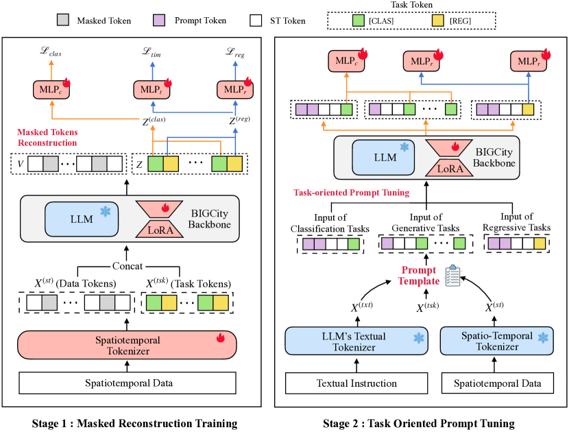
Figure 4: The hierarchical training strategy of BIGCity.

VI Model Training

As shown in Fig. 4, BIGCity adopts a two-stage training strategy comprising Masked Reconstruction Training and Multi-Task Prompt Tuning. In the first stage, masked reconstruction training, a self-supervised approach is employed to enable the model to learn general spatiotemporal dependencies from ST sequence data. In the second stage, multi-task prompt tuning, a multi-task co-training method is utilized to allow the model to handle a variety of tasks within a unified framework, eliminating the need for task-specific fine-tuning.

VI-A Masked Reconstruction Training

In this stage, we employ a masked reconstruction task to enable the model to capture general features of ST sequences without being tailored to specific data analysis tasks. Masked reconstruction is a widely used approach in LLM pre-training, where certain samples from the input sequence are randomly masked, and the model predicts the masked samples. This task allows the model to learn intrinsic correlations within the input sequence data without requiring labeled data. The specific process of masked reconstruction training in our model is described as follows.

Inputs. Given an ST-unit sequence corresponding to a trajectory or traffic state series, i.e., $\mathcal{U}=(\bm{U}_{1},\cdots,\bm{U}_{L})$, the ST tokenizer encodes it into an ST token sequence $\bm{X}^{(\mathrm{st})}=(\bm{x}_{1},\ldots,\bm{x}_{L})$. We randomly mask $K$ tokens in $\bm{X}^{(\mathrm{st})}$, replacing them with the mask token $[\mathrm{MASK}]$, resulting in $\tilde{\bm{X}}^{(\mathrm{st})}=(\bm{x}_{1},\cdots,[\mathrm{MASK}]_{1},\cdots,\bm{x}_{l},\cdots,[\mathrm{MASK}]_{K},\cdots,\bm{x}_{L})$. For each $[\mathrm{MASK}]_{k}$, we assign a task placeholder pair $([\mathrm{CLAS}]_{k},[\mathrm{REG}]_{k})$, producing a task token sequence:

$$\small\bm{X}^{(\mathrm{tsk})}=\left(\big{(}\bm{x}_{1}^{(\mathrm{clas})},\bm{x}_{1}^{(\mathrm{reg})}\big{)},\ldots,\big{(}\bm{x}_{K}^{(\mathrm{clas})},\bm{x}_{K}^{(\mathrm{reg})}\big{)}\right).$$ (12)

Finally, the token sequence $\bm{\mathcal{X}}=\big{(}\tilde{\bm{X}}^{(\mathrm{st})},\bm{X}^{(\mathrm{tsk})}\big{)}$ is fed into the backbone LLM model for masked reconstruction training.

Outputs. Given $\bm{\mathcal{X}}$ as input to the backbone model, the output is a result token sequence $\bm{Z}$, where each element corresponds one-to-one with elements in $\bm{X}^{(\mathrm{tsk})}$, as follows:

$$\small\bm{Z}=\left(\big{(}\bm{z}_{1}^{(\mathrm{clas})},\bm{z}_{1}^{(\mathrm{reg})}\big{)},\ldots,\big{(}\bm{z}_{K}^{(\mathrm{clas})},\bm{z}_{K}^{(\mathrm{reg})}\big{)}\right).$$ (13)

For the $k$-th output token $\big{(}\bm{z}_{k}^{(\mathrm{clas})},\bm{z}_{k}^{(\mathrm{reg})}\big{)}$, the general-task head (Eq. (11)) decodes it into an predicted ST-unit:

$$\small\hat{\mathcal{U}}_{k}=\left(\hat{\bm{y}}_{k}^{(\mathrm{clas})},\hat{\bm{y}}_{k}^{(\mathrm{reg})},\hat{y}_{k}^{(\mathrm{tim})}\right),$$ (14)

which represents the reconstructed sample for the ST-unit masked by $[\mathrm{MASK}]_{k}$. In Eq. (14), $\hat{\bm{y}}_{k}^{(\mathrm{clas})}$ is the predicted road segment ID, $\hat{\bm{y}}_{k}^{(\mathrm{reg})}$ is the predicted dynamic feature of the road segment, and $\hat{y}_{k}^{(\mathrm{tim})}$ is the predicted timestamp.

Loss Function. We employ the Cross-Entropy loss for classification and the Mean Squared Error (MSE) loss for regression. For each masked ST-unit, there are three losses:

$$\;\;\;\mathcal{L}_{\mathrm{clas}}=\sum_{k=1}^{K}\bm{\phi}\Big{(}r_{k}\Big{)}\log\left(\hat{\bm{y}}_{k}^{(\mathrm{clas})}\right),$$ (15)

$$\mathcal{L}_{\mathrm{reg}}=\sum_{k=1}^{K} \left\|\bm{e}^{(d)}_{k}-\hat{\bm{y}}_{k}^{(\mathrm{reg})}\right\|^{2}_{F},\;\;\mathcal{L}_{\mathrm{tim}}=\sum_{k=1}^{K}\left(\tau_{k}-\hat{y}_{k}^{(\mathrm{tim})}\right)^{2},$$

where $\bm{\phi}\big{(}r_{k}\big{)}$, $\bm{e}^{(d)}_{k}$, and $\tau_{k}$ are the ground truths for $\hat{\mathcal{U}}_{k}$. The final loss function for masked reconstruction training is:

$$\small\mathcal{L}_{\mathrm{MRT}}=\frac{1}{K\times N}\sum_{n=1}^{N}\left(\mathcal{L}_{\mathrm{clas}}^{(n)}+\lambda_{1}\mathcal{L}_{\mathrm{reg}}^{(n)}+\lambda_{2}\mathcal{L}_{\mathrm{tim}}^{(n)}\right),$$ (16)

where $\lambda_{1}$ and $\lambda_{2}$ are predefined parameters, the superscript $(n)$ indicates the index of a training sample, and $N$ is the total number of training samples.

During Masked Reconstruction Training, the ST tokenizer and the LoRA module in the backbone are jointly trained by minimizing the loss function $\mathcal{L}_{\mathrm{MRT}}$.

VI-B Task-oriented Prompt Tuning

This stage trains our model to perform various ST data analysis tasks using task-oriented prompts.

Inputs. In this stage, the inputs are task-oriented prompts for diverse tasks. Datasets for all task types are combined into a unified training dataset, referred to as the full training set. For each sample in the full training set, a corresponding prompt is generated as $\bm{\mathcal{X}}=\big{(}\bm{X}^{(\mathrm{txt})},\bm{X}^{(\mathrm{st})},\bm{X}^{(\mathrm{tsk})}\big{)}$, which serves as the input to the backbone model of BIGCity.

In the implementation, we incorporate three types of tasks for prompt tuning: classification, regression, and generation. The textual instruction tokens $\bm{X}^{(\mathrm{txt})}$ in $\bm{\mathcal{X}}$ follow fixed templates as shown in Fig. 3. The data tokens $\bm{X}^{(\mathrm{st})}$ and task tokens $\bm{X}^{(\mathrm{tsk})}$ for these tasks are described as follows:

• Classification Tasks include next hop prediction and trajectory classification. Trajectory classification tasks further comprise trajectory traffic pattern classification and user-trajectory linkage. The data tokens $\bm{X}^{(\mathrm{st})}$ in $\bm{\mathcal{X}}$ represent a sequence of ST-units corresponding to a trajectory. The task tokens $\bm{X}^{(\mathrm{tsk})}$ consist of a single $[\mathrm{CLAS}]$, corresponding to the class label to be predicted.

• Regression Tasks include travel time estimation and traffic state prediction. $i$) For the travel time estimation task, the data tokens $\bm{X}^{(\mathrm{st})}$ are a trajectory ST-unit sequence, where timestamps at locations with unknown travel times are replaced by $[\mathrm{MASK}]$. The task tokens are a sequence of $[\mathrm{REG}]$, each corresponding to an unknown timestamp. $ii$) For traffic state prediction, the data tokens represent the first half of a traffic state sequence, and the task tokens are a sequence of $[\mathrm{REG}]$, each corresponding to the rest traffic state steps to be predicted.

• Generation Task includes trajectory recovery. The data tokens consist of a low-sampling-rate trajectory where locations to be recovered are inserted with $[\mathrm{MASK}]$. The task tokens are a sequence of $[\mathrm{CLAS}]$ with the same number of elements as the $[\mathrm{MASK}]$ tokens. Each $[\mathrm{CLAS}]$ corresponds to a sample to be recovered in the low-sampling-rate trajectory.

Outputs. For classification tasks, the general-task heads decode the output token corresponding to $[\mathrm{CLAS}]$ into the predicted class label. For regression tasks, the output token corresponding to $[\mathrm{REG}]$ is decoded into predicted timestamps or traffic states. For generation tasks, the output tokens corresponding to $[\mathrm{CLAS}]$ are decoded into the road segment IDs of the recovered samples.

Loss Function. In task-oriented prompt tuning, we use samples from all tasks, i.e., the full training set, to co-train the model. The overall loss function is defined as:

$$\mathcal{L}_{\mathrm{PT}}=\mathcal{L}_{\mathrm{CLAS}}+\lambda_{2}\mathcal{L}_{\mathrm{REG}}+\lambda_{3}\mathcal{L}_{\mathrm{GEN}},$$ (17)

where $\mathcal{L}_{\mathrm{CLAS}}$, $\mathcal{L}_{\mathrm{REG}}$, and $\mathcal{L}_{\mathrm{GEN}}$ represent the loss functions for classification, regression, and generation tasks, respectively. Cross-entropy loss is applied for classification tasks, while mean squared error (MSE) loss is used for regression tasks.

In task-oriented prompt tuning, only the parameters in the LoRA modules of the backbone model are updated using the loss function $\mathcal{L}_{\mathrm{PT}}$, while the parameters of the ST tokenizer remain frozen. After completing both the masked reconstruction training and task-oriented prompt tuning, the ST tokenizer and the VMTP are assembled to form the complete BIGCity model, capable of ST data analysis across multiple tasks in multiple data modalities (MTMD).

TABLE I: Types of ST Data Analysis Tasks

Task Type	Trajectory Based	Traffic State Based
Classification	Next Hop Prediction	\
	Trajectory Classification
Regression	Travel Time Estimation	One-Step Prediction
		Multi-Step Prediction
Comparison	Most Similar Search	\
Generation	Trajectory Recovery	Traffic State Imputation

TABLE II: Statistics of the Three Datasets.

Dataset	BJ	XA	CD
Time Span	one month	one month	one month
Trajectory	1018312	384618	559729
User Number	1677	26787	48295
Road Segments	40306	5269	6195

TABLE III: Performance on the trajectory-based non-generative tasks, i.e., Travel Time Estimation, Trajectory Classification, Trajectory Next Hop Prediction, Most Similar Trajectory Search. Particularly, MAPE here are percentage numbers.

Task		Travel Time Estimation			Trajectory Classification			Next Hop Prediction			Most Similar Search
Data	Model	MAE$\downarrow$	RMSE$\downarrow$	MAPE$\downarrow$	ACC$\uparrow$	F1$\uparrow$	AUC$\uparrow$	ACC$\uparrow$	MRR@5$\uparrow$	NDC@5 $\uparrow$	HR@1$\uparrow$	HR@5$\uparrow$	HR@10$\uparrow$
BJ	Tr2v	10.13	56.83	37.95	0.811	0.852	0.837	0.633	0.746	0.784	0.607	0.766	0.867
	T2v	10.03	56.65	36.42	0.814	0.863	0.879	0.623	0.731	0.769	0.788	0.885	0.932
	TBR	9.981	36.97	34.25	0.818	0.876	0.871	0.537	0.625	0.659	0.396	0.499	0.538
	Toa	10.79	57.41	35.37	0.821	0.861	0.862	0.714	0.841	0.878	0.326	0.399	0.767
	JCL	10.23	46.49	41.22	0.808	0.859	0.873	0.714	0.841	0.881	0.531	0.699	0.936
	STA	9.156	35.41	32.01	0.853	0.885	0.905	0.734	0.836	0.882	0.776	0.878	0.934
	JRM	10.18	41.88	39.51	0.849	0.879	0.897	0.746	0.843	0.896	0.681	0.852	0.906
	Ours	8.869	33.21	30.34	0.872	0.891	0.909	0.751	0.855	0.902	0.801	0.895	0.952
Data	Model	MAE$\downarrow$	RMSE$\downarrow$	MAPE$\downarrow$	Mi-F1$\uparrow$	Ma-F1$\uparrow$	Ma-Re$\uparrow$	ACC$\uparrow$	MRR@5$\uparrow$	NDC@5$\uparrow$	HR@1$\uparrow$	HR@5$\uparrow$	HR@10$\uparrow$
XA	Tr2v	2.051	3.147	35.14	0.086	0.085	0.093	0.679	0.759	0.788	0.673	0.854	0.889
	T2v	2.035	3.132	33.73	0.086	0.082	0.089	0.672	0.747	0.774	0.733	0.821	0.877
	TBR	2.016	3.121	32.13	0.091	0.088	0.081	0.568	0.633	0.657	0.538	0.67	0.725
	Toa	2.152	3.266	33.93	0.099	0.095	0.092	0.778	0.887	0.913	0.283	0.393	0.442
	JCL	2.173	3.257	33.12	0.093	0.091	0.095	0.793	0.889	0.919	0.335	0.551	0.634
	STA	1.833	2.982	30.57	0.101	0.098	0.102	0.825	0.903	0.928	0.741	0.883	0.893
	JRM	1.915	3.152	31.88	0.097	0.094	0.097	0.829	0.906	0.934	0.703	0.826	0.863
	Ours	1.723	2.614	29.76	0.112	0.104	0.113	0.837	0.923	0.942	0.791	0.887	0.909
Data	Model	MAE$\downarrow$	RMSE$\downarrow$	MAPE$\downarrow$	Mi-F1$\uparrow$	Ma-F1$\uparrow$	Ma-Re$\uparrow$	ACC$\uparrow$	MRR@5$\uparrow$	NDC@5$\uparrow$	HR@1$\uparrow$	HR@5$\uparrow$	HR@10$\uparrow$
CD	Tr2v	1.635	2.432	34.74	0.142	0.152	0.156	0.726	0.809	0.837	0.607	0.748	0.794
	T2v	1.632	2.433	34.45	0.149	0.151	0.158	0.711	0.791	0.819	0.543	0.715	0.753
	TBR	1.620	2.405	34.15	0.142	0.156	0.155	0.608	0.682	0.708	0.409	0.532	0.576
	Toa	1.708	2.493	37.23	0.143	0.152	0.153	0.789	0.872	0.911	0.225	0.322	0.357
	JCL	1.657	2.481	36.42	0.148	0.164	0.157	0.792	0.881	0.904	0.348	0.552	0.642
	STA	1.433	2.394	32.12	0.151	0.163	0.159	0.795	0.885	0.919	0.607	0.757	0.776
	JRM	1.372	2.253	30.79	0.143	0.152	0.151	0.798	0.888	0.927	0.631	0.774	0.815
	Ours	1.287	2.181	28.59	0.153	0.169	0.162	0.821	0.912	0.938	0.646	0.787	0.821

• The bold results are the best, and the underlined results are the second best. The metric with ”$\uparrow$” (”$\downarrow$”) means that a larger (smaller) result is better.

TABLE IV: Performance on trajectory based generative tasks, i.e., Trajectory Recovery. $85\%$, $90\%$, and $95\%$ are masked ratios.

Metric	Accuracy $\uparrow$									Macro-F1 $\uparrow$
	BJ			XA			CD			BJ			XA			CD
	85%	90%	95%	85%	90%	95%	85%	90%	95%	85%	90%	95%	85%	90%	95%	85%	90%	95%
Linear+HMM	0.219	0.205	0.196	0.275	0.239	0.207	0.289	0.268	0.233	0.098	0.095	0.089	0.125	0.101	0.094	0.131	0.117	0.099
DTHR+HMM	0.236	0.227	0.208	0.269	0.218	0.201	0.296	0.264	0.224	0.118	0.097	0.091	0.135	0.121	0.105	0.141	0.119	0.106
MTrajRec	0.456	0.418	0.323	0.495	0.443	0.338	0.512	0.459	0.347	0.201	0.177	0.136	0.221	0.199	0.145	0.244	0.240	0.164
RNTrajRec	0.475	0.439	0.338	0.503	0.456	0.359	0.523	0.478	0.369	0.205	0.181	0.152	0.267	0.226	0.173	0.292	0.257	0.185
Ours	0.518	0.471	0.368	0.562	0.489	0.381	0.585	0.513	0.405	0.259	0.217	0.177	0.309	0.258	0.194	0.321	0.269	0.212

TABLE V: The Performance in Traffic State Tasks

Data	XA
Task	One-Step			Multi-Step			Imputation
Metric	MAE	MAPE	RMSE	MAE	MAPE	RMSE	MAE	MAPE	RMSE
DCR	1.092	11.77	2.312	1.293	16.38	2.492	0.585	7.493	1.403
GWN	1.113	11.44	2.264	1.304	15.59	2.331	0.847	10.63	1.833
MTG	1.072	10.56	1.903	1.223	14.91	2.163	0.906	11.12	1.790
TrG	1.103	11.46	2.042	1.263	15.90	2.423	0.944	11.79	1.815
STG	1.122	12.59	2.272	1.392	17.34	2.304	0.989	12.40	1.709
STN	0.974	10.27	1.973	1.268	15.64	2.281	0.940	11.64	1.789
SST	0.802	9.972	1.873	1.183	14.21	2.292	0.883	11.23	1.736
Ours	0.791	9.732	1.743	1.162	14.01	2.143	0.536	6.671	1.335
Data	XA
Task	One-Step			Multi-Step			Imputation
Metric	MAE	MAPE	RMSE	MAE	MAPE	RMSE	MAE	MAPE	RMSE
DCR	1.232	13.02	2.324	1.552	18.22	2.862	0.731	8.601	1.704
GWN	1.342	12.71	2.414	1.612	18.14	2.713	1.024	11.80	2.121
MTG	1.183	11.93	2.132	1.413	16.76	2.506	1.109	12.71	2.055
TrG	1.234	12.39	2.312	1.562	17.69	2.761	1.165	13.14	2.082
STG	1.352	12.91	2.413	1.633	18.77	2.603	1.235	14.37	2.046
STN	1.203	11.99	2.201	1.491	17.02	2.594	1.152	12.88	2.061
SST	1.163	11.77	2.191	1.452	17.01	2.954	1.027	11.84	2.005
Ours	1.122	11.16	2.103	1.412	15.98	2.471	0.665	8.192	1.617

VII Experiments

VII-A Experimental Setting

Spatiotemporal (ST) Tasks. As a multi-task model, BIGCity is co-trained on four types of ST tasks, and simultaneously tackling eight specific tasks, as listed in Tab. I. While current baselines demands individual training for each task.

Datasets. We evaluated BIGCity on three real-world datasets: Beijing (BJ), Xi’an (XA), and Chengdu (CD). The BJ dataset consists of taxi trajectories collected in November 2015 [16], while the XA and CD datasets include online car-hailing trajectories from November 2018, provided by the DiDi GAIA project. Road networks for all three cities were extracted from OpenStreetMap (OSM), and trajectories were map-matched to the networks to compute traffic states. Each time slice for traffic states spans 30 minutes. Due to sparse trajectories in the BJ dataset, dynamic traffic state features from ST units (Eq. (2)) were excluded, a limitation common in trajectory datasets. For experiments, XA and CD datasets were split $6:2:2$ for training, validation, and testing, while BJ was split $8:1:1$. Dataset statistics are provided in Tab. II. In addition, our data are processed by libcity [93]

Baselines. BIGCity is evaluated by comparing with seventeen task-specific baselines of each particular task. For classification, regression and comparison tasks of trajectory input, we select the seven current state-of-art (SOTA) trajectory representation models: Trajectory2vec (Tr2v) [10], T2vec (T2v) [94], TremBR (TBR) [14], Toast (Toa) [11], JCLRNT (JCL) [12], START (STA) [15], and JGRM (JRM) [13]. For traffic state input, BIGCity is compared with six current SOTA traffic state prediction models: DCRNN [43], GWNET [45], MTGNN [17], TrGNN [18], STGODE [95], ST-Norm[19], and SSTBAN [20]. Table V. For generation tasks, BIGCity is compared with four recovery models: Linear+HMM [1], DTHR+HMM, MTrajRec [96], and RNTrajRec [97].

Evaluation Metrics. For trajectory Travel Time Estimation: we adopt three metrics, including mean absolute error (MAE), mean absolute percentage error (MAPE), and root mean square error (RMSE); For next hop prediction: Following the settings in [16], we used three metrics: Accuracy (ACC), mean reciprocal rank at 5 (MRR@5) and Normalized Discounted Cumulative Gain at 5 (NDCG@5); For trajectory classification: We use Accuracy (ACC), F1-score (F1), and Area Under ROC (AUC) to evaluate binary classification on BJ dataset. Using Micro-F1, Macro-F1 and Macro-Recall on XA and CD datasets; For most similar trajectory search: we evaluated the model using Top-1 Hit Rate (HR@1), Top-5 Hit Rate (HR@5), and Top-10 Hit Rate (HR@10), where Top-k Hit rate indicates the probability that the ground truth is in the top-k most similar samples ranked by the model; Metrics used in traffic state tasks are: MAE, MAPE, RMSE; For trajectory Recovery: We evaluated our model on three types of mask ratios: $85\%$, $90\%$, $95\%$. The evaluation metric is the recovery accuracy and Macro-F1 on masked road segments.

Implementation Details. We chose GPT-2 as our backbone, and conducted experiments on Ubuntu 20.04 using 4 NVIDIA H800 80GB GPUs with pytorch 1.8.1. The implementation of our model can be find in code .

VII-B Performance Comparison

We conducted extensive experiments on all 3 datasets across 8 ST tasks. As current baselines handle trajectories and traffic states separately, we compared BIGCity to trajectory and traffic state baselines individually. All comparison experiments are repeated ten times, we list the mean values in this paper and provide standard deviation in the code link.

Trajectory Tasks. Firstly, we conclude trajectory next-hop prediction (Next), travel time estimation (TTE), trajectory classification (CLAS), and similar trajectory search (Simi) as trajectory-based non-generative tasks as these four tasks share similar pipelines. Notably, current baselines require individual training on each task, while BIGCity handles these tasks with a single set of parameters. Following the settings in [13], Next task prediction the next token of an input, In TTE, we mask off all timestamps, and the ground truth for each segment is the time interval between its former one segment. Simi takes a certain input samples as queries and search the most similar samples from the whole dataset, and more details please refer to [13]. CLAS in BJ is a binary classification. In XA and CD, CLAS is a user-trajectory link classification and we only retained users with more than 50 trajectories. The comparison results are given in Tab. III. BIGCity consistently and significantly outperforms the baselines across all scenarios.

Subsequently, trajectory recovery (Reco) usually employs task-specific models. For each input data, we sample it at a specific frequency to obtain a low-frequency trajectory and use the original trajectory as the target for trajectory recovery. We evaluate model’s performance under different mask ratios. The comparison results are given in Tab. IV.

TABLE VI: Generalization experiments on three tasks, i.e., travel time estimation, next hop prediction (Next), trajectory classification (CLAS)

Data	Tasks	TTE		Next		CLAS
		MAE$\downarrow$	RMSE$\downarrow$	ACC$\uparrow$	MRR@5$\uparrow$	Mi-F1$\uparrow$	Ma-F1$\uparrow$
XA	BIGCity	1.72	2.61	0.837	0.923	0.110	0.104
	BIG-BJ	1.82	2.78	0.806	0.912	0.103	0.097
	Loss	5.89%	5.98%	3.81%	1.20%	6.46%	6.94%
CD	BIGCity	1.29	2.18	0.821	0.910	0.153	0.169
	BIG-BJ	1.37	2.31	0.792	0.878	0.144	0.159
	Loss	5.63%	5.72%	3.62%	1.12%	6.22%	6.15%

Traffic State Tasks. We evaluate BIGCity on three traffic state tasks, i.e., one-step prediction (O-Step), multi-step prediction (M-Step), and traffic state imputation (TSI). Specifically, one-step prediction generates the traffic state in the next time slice, and multi-step prediction generates traffic states in the next 6 time slice. In traffic state imputation, we masked $25\%$ input data and trained models to recovery the masked data. Here, we only conducted experiments on XA and CD, as the trajectories in BJ are too sparse to get reliable traffic states. As shown in Tab. V, our model largely outperforms the other baselines for both one-step and multi-step predictions on the two datasets. The average performance advantage is $\bm{2.83}\%$, with the largest reaching $\bm{7}\%$. As for traffic state imputation, the average and largest improvement are $\bm{7.8}\%|\bm{12.3}\%$.

In above experiments, BIGCity outperforms 17 baselines (7 representation models and 10 task-specific models) across all tasks, datasets, and metrics, indicating its universality and robust multi-task ability.

VII-C Generalization Ability

We evaluate BIGCity’s generalization ability in across datasets scenario. Specifically, we first trained the whole BIGCity on BJ dataset. Then, we transfer BIG-BJ’s backbone model to XA and CD dataset. Specifically, we combined the spatiotemporal tokenizer of XA and CD with the backbone trained on BJ, and only fine-tuned the last MLP layer of tokenizers on XA and CD datasets. The experimental results are given in Tab. VI. In both XA and CD, BIGCity-BJ denotes the transferred model with its backbone trained on BJ, and BIGCity is the model completely trained on XA or CD. The generalization ability is evaluated by the performance loss between BIGCity and BIG-BJ. As shown in the table, the average performance degradation for BIGCity-BJ compared with original BIGCity model is within $\bm{7}\%$. In comparison with the results in Tab. III, BIGCity-BJ still outperforms all of baselines in most cases, demonstrating our BIGCity’s superior cross-city generalization capability as well as the robustness. The experimental results indicate that our model has potential to be applied in a valuable scenario: pre-training the backbone model on a large city with ample data and then transferring it to smaller cities with limited data.

VII-D Ablation Studies

We consider the superior performance of BIGCity stems from two key factors: $\bf{1)}$ The general representation captures comprehensive ST features, and $\bf{2)}$ the co-training mechanism in task-oriented tuning enhances ST feature sharing across tasks. In this section, we conduct analysis on the above hypotheses and evaluate the contributions of each module. Specifically, we first conducted ablations on model designs, followed by ST co-training mechanism. All experiments are conducted on the XA dataset. Notably, some modules are essential to certain tasks. For example, there won’t be trajectory tasks if the static encoder is absent. In Tab. VII and Tab. VIII, ${}^{\prime}-^{\prime}$ denotes such tasks.

Ablations on Model Designs. We first conducted ablations on the static encoder, dynamic encoder of the spatiotemporal tokenizer, thereby evaluating the contribution of general representation. Subsequently, we conduct ablations on task-oriented prompts. Specifically, $\bf{1}$) w/o-Dyn removes the dynamic encoder, resulting in the loss of dynamic traffic state information. $\bf{2}$) w/o-Sta removes the static encoder, resulting in the loss of static topology information. $\bf{3}$) w/o-Fus removes the fusion encoder, resulting in the loss of long-range ST features integration. $\bf{4)}$w/o-Pro removes prompts from the input, and we trained a specific task MLP for each individual task. As shown in Tab. VII, the fusion encoder benefits all ST tasks, especially in tasks prefer long-range ST dependencies, i.e., travel time estimation. Results in w/o-Sta and w/o-Dyn indicate that the general representation indeed enhances BIGCity’s performance. Dynamic features enhance trajectory tasks by improving representational distinctiveness, while static features benefit traffic state tasks by incorporating long-range topology information through input trajectories. As for task-oriented prompts, they have the most significant influence on performance of all tasks.The experimental results demonstrate their importance in BIGCity’s multi-task ability, as they provide task-specific guidance.

Ablations on Training. We consider multi-task co-training benefits BIGCity in feature exchanges among tasks. Therefore, we conduct ablations on threehighly heterogeneous tasks, i.e., next hop prediction (Next), travel time estimation (TTE), multi-step traffic state prediction (MS). All denotes co-trained all three tasks. We incrementally add the task type for multi-task co-training. Experimental results in Tab. VIII indicate that: the greater the differences in task types and data features (multi-step prediction and next hop prediction), the more significant the model’s gains from multi-task co-training.

TABLE VII: Ablation Studies on Model Designs

Task	TTE	CLAS	Next	Simi.	Reco.	TSI	M-Step	AveGAP
	MAE↓	Ma-F1 ↑	Acc ↑	HR10 ↑	Acc. ↑	MAPE↓	MAPE↓
w/o-Dyn+Fus	1.96	0.102	0.803	0.801	0.537	-	-	-
GAP	13.9%	2.2%	4.1%	11.8%	4.4%	-	-	7.28
w/o-Dyn	1.87	0.102	0.815	0.805	0.550	-	-	-
GAP	11.7%	2.2%	2.7%	11.4%	2.2%	-	-	6.9%
w/o-Sta+Fus	-	-	-	-	-	7.18	14.83	-
GAP	-	-	-	-	-	6.8%	4.9%	5.8%
w/o-Sta	-	-	-	-	-	7.02	14.48	-
GAP	-	-	-	-	-	5.3%	3.4%	4.4%
w/o-Pro	2.03	0.096	0.759	0.892	0.513	7.672	15.51	-
GAP	18.0%	11.5%	9.3%	1.8%	8.7%	15.0%	9.6%	10.5%
BIGCity	1.72	0.104	0.837	0.909	0.562	6.671	14.01	-

TABLE VIII: Ablation Studies on ST Tasks. MS denotes the multi-step traffic state prediction tasks

Metric	Task
	Next	TTE	MS	MS+Next	TTE+Next	All
ACC $\uparrow$	0.79	-	-	0.82	0.8	0.84
MAE $\downarrow$	-	1.8	-	-	1.77	1.75
MAPE $\downarrow$	-	-	14.36	14.19	-	14.14

VIII Model Analysis

VIII-A Parameter Sensitivity

We conducted parameter sensitivity analysis for critical hyper-parameters, i.e., the quantity of LoRA modules as well as the matrix rank within each module. The rate of LoRA modules are denoted as $n$, and the matrix rank in each LoRA module is denoted as $r$. We set $n$ to $1$, $1/2$, and $1/3$. For example, $n=1/2$ means the there are $50\%$ of GPT-2’s attention blocks are attached with LoRA modules. The range of $r$ is $4$, $8$, $16$, $32$.

Specifically, we conduct analysis on three types of tasks, i.e., regression task (travel time estimation), classification task (next hop prediction), comparison task (most similar search). The results of travel time estimation are presented in Fig. 5(a) and Fig. 5(d). Since smaller MAE and MAPE means better model performance, we use $\frac{10}{MAE}$ and $\frac{10}{RMSE}$ on the vertical axis to represent MAE and MAPE, respectively. The results in next hop prediction are in Fig. 5(b) and Fig. 5(f), where Accuracy and MRR@5 are metrics. The results in most similar trajectory search are in Fig. 5(c) and Fig. 5(f), where HR@1 and HR@5 are metrics. The experimental results show that model’s performance improves with increasing $n$. However, BIGCity is more sensitive to $r$. When $r\leq 8$, the model’s performance increases with $r$, but for $r\geq 16$, the performance deteriorates as $r$ continues to rise. Considering both computational cost and performance, we selected $n=1$ and $r=8$.

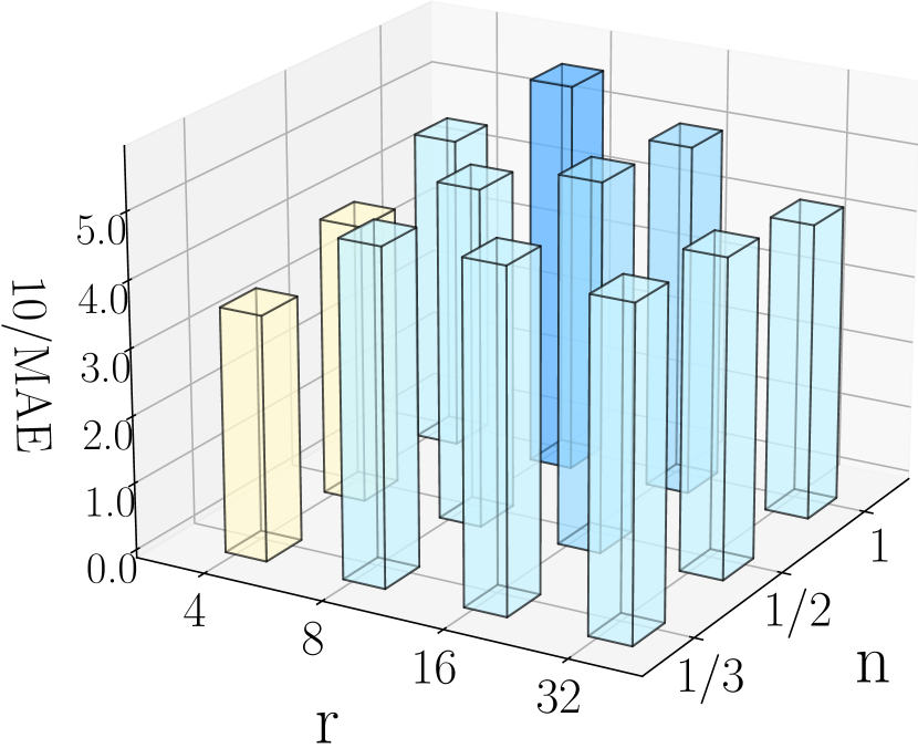
(a) MAE on travel time estimation task

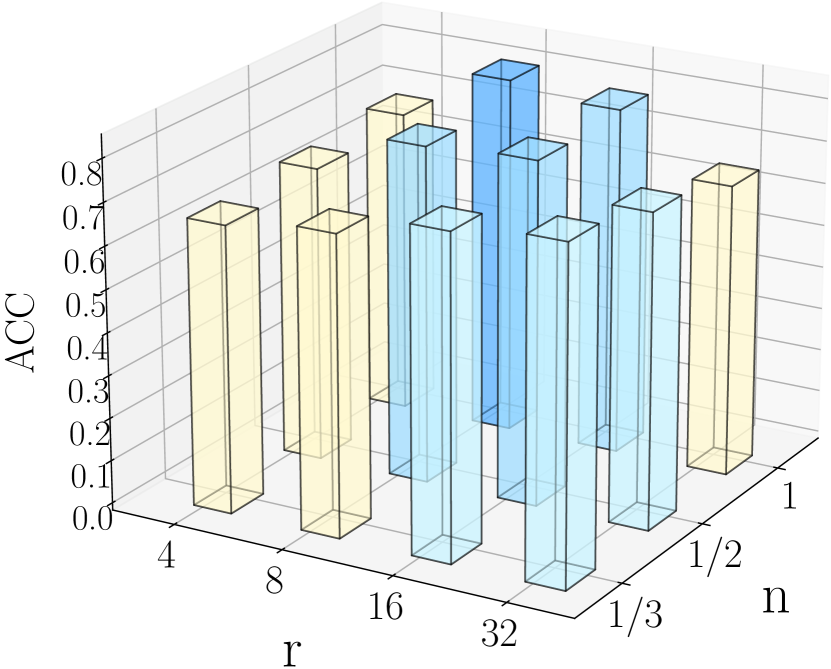
(b) Accuracy on next hop prediction task

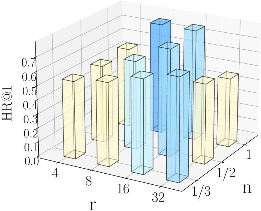
(c) HR@1 on most similar search task

(d) RMSE on travel time estimation task

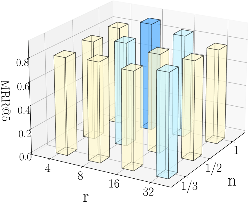
(e) MRR@5 on next hop prediction task

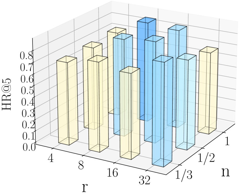
(f) HR@5 on most similar search task

Figure 5: The parameter sensitivity analysis on classification, regression, and comparison task

VIII-B Model Efficiency And Scalability

We conducted efficiency and scalability experiments on thr XA dataset, with the number of input samples increase from $100$k to $350$k. The experimental results are shown in Fig. 6. Similar trends are observed in other datasets.

TABLE IX: The Efficiency Analysis on XA. Stage-1 is the representation training, Stage-2 is the task-related tuning

Models	GPU Usage (GB)	Stage-1 Speed (min/epoch)	Stage-2 Speed (min/epoch)
Traj2vec	4.932	4.662	3.761
Toast	5.271	4.801	3.996
START	21.65	14.93	7.753
BIGCity	28.73	11.32	8.681

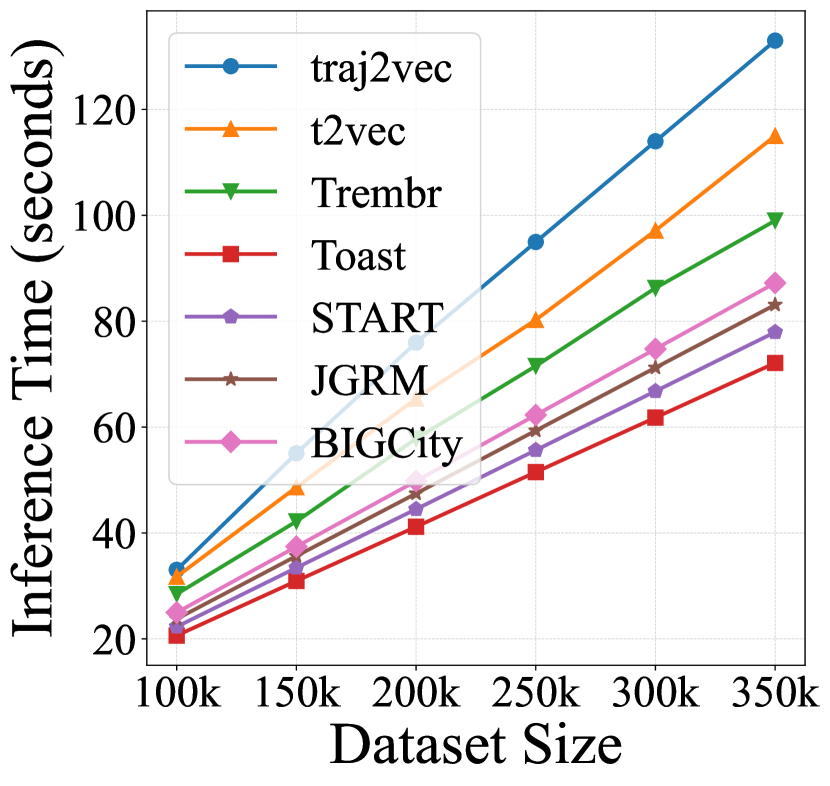
(a) Efficiency: Inference Time

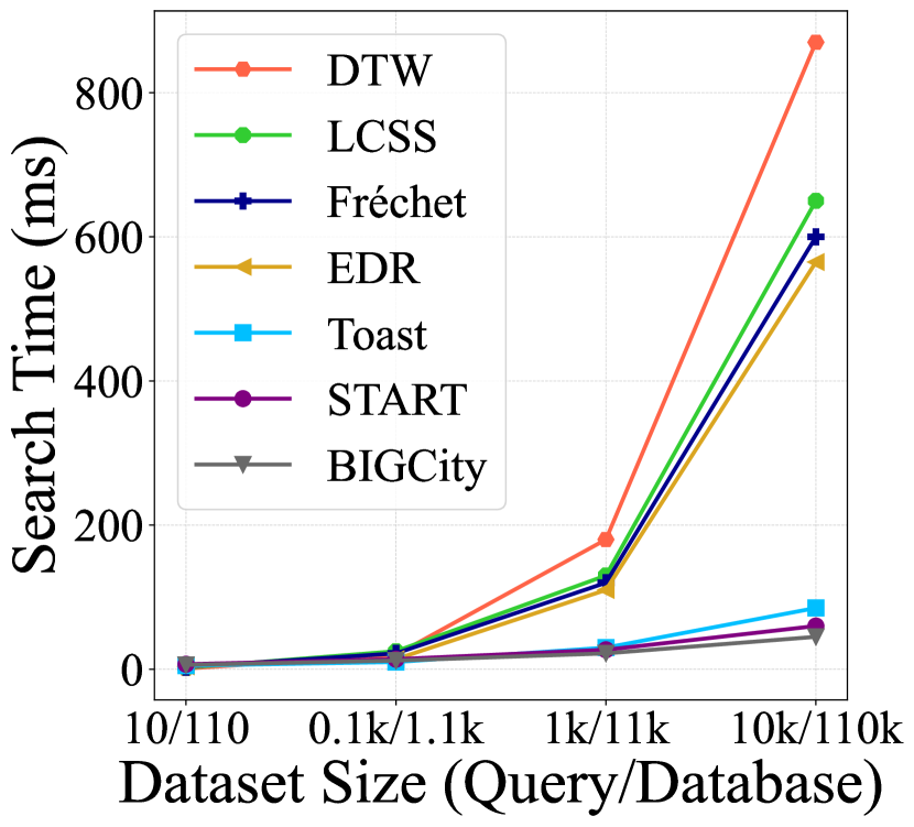
(b) Scalability: Search Time

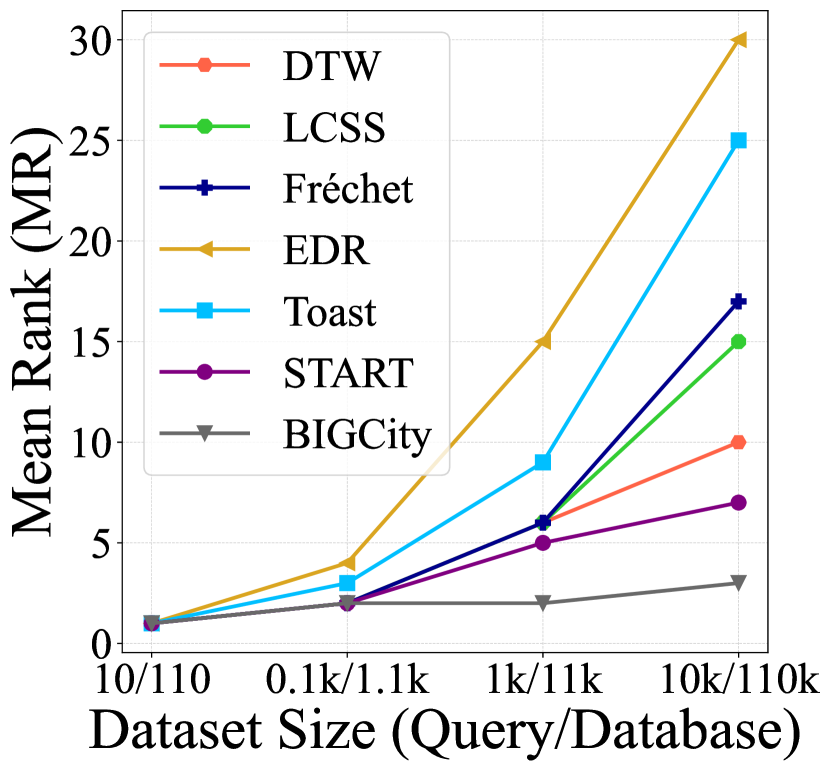
(c) scability: Performace

Figure 6: (a) Inference Efficiency: Time required to generate ST representations as data size grows. (b) Average Search Time: Time taken for query searches as data size grows. (c) Mean Rank: Average rank of ground truth in similarity-based sorting; lower is better.

Efficiency. Although with the largest parameter size, BIGCity still demonstrates the efficiency advantage as a multi-task model in both training and inference time cost.

For training, we compare BIGCity with those two-stage training baselines on travel time estimation task. As a two-stage training model, we consider training cost of both stage 1 (representation training) and stage 2 (task tuning). We provide GPU usage, Training speed in stage 1, and stage 2. As shown in Tab. IX, BIGCity has the largest parameter size but with moderate training cost. Even in stage 1, BIGCity is faster than the smaller model like START. This is because we trained BIGCity by LoRA, ensuring that there is a reasonable trade-off between additional learnable parameters and training speed.

For inference, we record the time cost of representing $100$k–$350$k input samples by the backbone. As shown in Fig 6(a), BIGCity outperform RNN models in speed while having the speed similar to models with three times fewer parameters [16]. BIGCity has the largest parameters yet maintains moderate inference cost. This is because: $\bm{1)}$ The RNN model operates sequentially, whereas the attention mechanism in BIGCity is parallel. $\bm{2)}$ The causal attention mechanism in BIGCity has lower computational cost than self-attention, yet most baselines employ self-attention.

Scalability. In the sequel, we explore the scalability performance of BIGCity compared with six baselines, focusing on their ability to handle variations in dataset size. We conducted experiments on the most similar trajectory search task. It is suitable to demonstrate model scalability, as the volume of input data has significant influence on model’s performance and efficiency. We conduct experiments on inference time and performance in Fig 6(b) and Fig. 6(c). Specifically, the size of query sample varies from 10 to 10000, and the size of overall data is ten times of query samples. Besides SOTA deep learning baselines, we also involve some traditional algorithm. including Dynamic Time Warping (DTW) [98], Longest Common SubSequence (LCSS) [99], Fr’echet Distance [100], and Edit Distance on Real Sequence (EDR) [101]. As shown in Fig. 6(b), the inference cost of BIGCity linearly associates with the data volume but traditional methods is largely affected by data size. On the other hand, as shown in Fig. 6(c), BIGCity maintains robust performance with increasing data size. Unlike BIGCity, other baselines exhibit significant performance degradation. In summary, BIGCity is robust in performance and the computational cost linearly associates with the data volume. The experimental results indicate BIGCity has great potential in scaling to large datasets.

IX Conclusions

This study introduced the BIGCity model, a foundation model for urban spatiotemporal learning. By employing unified ST representations and textual prompts, BIGCity streamlined the processing of diverse spatiotemporal data and tasks within a single framework. Extensive experiments demonstrated BIGCity’s versatility and robustness. In addition, Although BIGCity has a large volume of parameters, it still demonstrates reasonable efficiency and impressive scalability. Future work: The current BIGCity model focused solely on road segments, excluding other spatial elements such as POIs and grids. We consider incorporating these elements is a promising direction for future research.

References

- [1] S. Hoteit, S. Secci, S. Sobolevsky, C. Ratti, and G. Pujolle, “Estimating human trajectories and hotspots through mobile phone data,” Computer Networks, vol. 64, pp. 296–307, 2014.
- [2] J. Ji, J. Wang, J. Wu, B. Han, J. Zhang, and Y. Zheng, “Precision cityshield against hazardous chemicals threats via location mining and self-supervised learning,” in Proceedings of the 28th ACM SIGKDD Conference on Knowledge Discovery and Data Mining, 2022, pp. 3072–3080.
- [3] Y. Chen, X. Li, G. Cong, Z. Bao, C. Long, Y. Liu, A. K. Chandran, and R. Ellison, “Robust road network representation learning: When traffic patterns meet traveling semantics,” in Proceedings of the 30th ACM International Conference on Information & Knowledge Management, 2021, pp. 211–220.
- [4] Z. Li, C. Huang, L. Xia, Y. Xu, and J. Pei, “Spatial-temporal hypergraph self-supervised learning for crime prediction,” in 2022 IEEE 38th International Conference on Data Engineering (ICDE). IEEE, 2022, pp. 2984–2996.
- [5] K. H. Hettige, J. Ji, S. Xiang, C. Long, G. Cong, and J. Wang, “Airphynet: Harnessing physics-guided neural networks for air quality prediction,” arXiv preprint arXiv:2402.03784, 2024.
- [6] J. Wang, X. Lin, Y. Zuo, and J. Wu, “Dgeye: Probabilistic risk perception and prediction for urban dangerous goods management,” ACM Transactions on Information Systems (TOIS), vol. 39, no. 3, pp. 1–30, 2021.
- [7] J. Wang, X. Wang, and J. Wu, “Inferring metapopulation propagation network for intra-city epidemic control and prevention,” in Proceedings of the 24th ACM SIGKDD international conference on knowledge discovery & data mining, 2018, pp. 830–838.
- [8] J. Wang, C. Chen, J. Wu, and Z. Xiong, “No longer sleeping with a bomb: a duet system for protecting urban safety from dangerous goods,” in Proceedings of the 23rd ACM SIGKDD International Conference on Knowledge Discovery and Data Mining, 2017, pp. 1673–1681.
- [9] Q. Gao, J. Hong, X. Xu, P. Kuang, F. Zhou, and G. Trajcevski, “Predicting human mobility via self-supervised disentanglement learning,” IEEE Transactions on Knowledge and Data Engineering, 2023.
- [10] D. Yao, C. Zhang, Z. Zhu, J. Huang, and J. Bi, “Trajectory clustering via deep representation learning,” in 2017 international joint conference on neural networks (IJCNN). IEEE, 2017, pp. 3880–3887.
- [11] Y. Chen, X. Li, G. Cong, Z. Bao, C. Long, Y. Liu, A. K. Chandran, and R. Ellison, “Robust road network representation learning: When traffic patterns meet traveling semantics,” in CIKM. ACM, 2021, pp. 211–220.
- [12] Z. Mao, Z. Li, D. Li, L. Bai, and R. Zhao, “Jointly contrastive representation learning on road network and trajectory,” in CIKM. ACM, 2022, pp. 1501–1510.
- [13] Z. Ma, Z. Tu, X. Chen, Y. Zhang, D. Xia, G. Zhou, Y. Chen, Y. Zheng, and J. Gong, “More than routing: Joint gps and route modeling for refine trajectory representation learning,” in Proceedings of the ACM on Web Conference 2024, 2024, pp. 3064–3075.
- [14] T.-Y. Fu and W.-C. Lee, “Trembr: Exploring road networks for trajectory representation learning,” ACM Transactions on Intelligent Systems and Technology (TIST), vol. 11, no. 1, pp. 1–25, 2020.
- [15] J. Jiang, D. Pan, H. Ren, X. Jiang, C. Li, and J. Wang, “Self-supervised trajectory representation learning with temporal regularities and travel semantics,” in 2023 IEEE 39th international conference on data engineering (ICDE). IEEE, 2023, pp. 843–855.
- [16] ——, “Self-supervised trajectory representation learning with temporal regularities and travel semantics,” in ICDE. IEEE, 2023.
- [17] Z. Wu, S. Pan, G. Long, J. Jiang, X. Chang, and C. Zhang, “Connecting the dots: Multivariate time series forecasting with graph neural networks,” in Proceedings of the 26th ACM SIGKDD international conference on knowledge discovery & data mining, 2020, pp. 753–763.
- [18] M. Li, P. Tong, M. Li, Z. Jin, J. Huang, and X.-S. Hua, “Traffic flow prediction with vehicle trajectories,” in Proceedings of the AAAI Conference on Artificial Intelligence, vol. 35, no. 1, 2021, pp. 294–302.
- [19] J. Deng, X. Chen, R. Jiang, X. Song, and I. W. Tsang, “St-norm: Spatial and temporal normalization for multi-variate time series forecasting,” in Proceedings of the 27th ACM SIGKDD conference on knowledge discovery & data mining, 2021, pp. 269–278.
- [20] S. Guo, Y. Lin, L. Gong, C. Wang, Z. Zhou, Z. Shen, Y. Huang, and H. Wan, “Self-supervised spatial-temporal bottleneck attentive network for efficient long-term traffic forecasting,” in 2023 IEEE 39th International Conference on Data Engineering (ICDE). IEEE, 2023, pp. 1585–1596.
- [21] Y. Liu, T. Hu, H. Zhang, H. Wu, S. Wang, L. Ma, and M. Long, “itransformer: Inverted transformers are effective for time series forecasting,” arXiv preprint arXiv:2310.06625, 2023.
- [22] Y. Yuan, J. Ding, J. Feng, D. Jin, and Y. Li, “Unist: A prompt-empowered universal model for urban spatio-temporal prediction,” arXiv preprint arXiv:2402.11838, 2024.
- [23] Z. Li, L. Xia, J. Tang, Y. Xu, L. Shi, L. Xia, D. Yin, and C. Huang, “Urbangpt: Spatio-temporal large language models,” arXiv preprint arXiv:2403.00813, 2024.
- [24] Z. Li, L. Xia, L. Shi, Y. Xu, D. Yin, and C. Huang, “Opencity: Open spatio-temporal foundation models for traffic prediction,” arXiv preprint arXiv:2408.10269, 2024.
- [25] Y. Zhu, J. J. Yu, X. Zhao, X. Wei, and Y. Liang, “Unitraj: Universal human trajectory modeling from billion-scale worldwide traces,” arXiv preprint arXiv:2411.03859, 2024.
- [26] Z. Zhou, Y. Lin, H. Wen, S. Guo, J. Hu, Y. Lin, and H. Wan, “Plm4traj: Cognizing movement patterns and travel purposes from trajectories with pre-trained language models,” 2024. [Online]. Available: https://arxiv.org/abs/2405.12459
- [27] P. Balsebre, W. Huang, G. Cong, and Y. Li, “Cityfm: City foundation models to solve urban challenges,” arXiv preprint arXiv:2310.00583, 2023.
- [28] W. X. Zhao, K. Zhou, J. Li, T. Tang, X. Wang, Y. Hou, Y. Min, B. Zhang, J. Zhang, Z. Dong et al., “A survey of large language models,” arXiv preprint arXiv:2303.18223, 2023.
- [29] T. Brown, B. Mann, N. Ryder, M. Subbiah, J. D. Kaplan, P. Dhariwal, A. Neelakantan, P. Shyam, G. Sastry, A. Askell et al., “Language models are few-shot learners,” Advances in neural information processing systems, vol. 33, pp. 1877–1901, 2020.
- [30] A. Radford, J. Wu, R. Child, D. Luan, D. Amodei, I. Sutskever et al., “Language models are unsupervised multitask learners,” OpenAI blog, vol. 1, 2019.
- [31] W. Wang, Q. Lv, W. Yu, W. Hong, J. Qi, Y. Wang, J. Ji, Z. Yang, L. Zhao, S. XiXuan et al., “Cogvlm: Visual expert for large language models,” 2023.
- [32] J. Jiang, C. Han, W. X. Zhao, and J. Wang, “Pdformer: Propagation delay-aware dynamic long-range transformer for traffic flow prediction,” in Proceedings of the AAAI conference on artificial intelligence, vol. 37, no. 4, 2023, pp. 4365–4373.
- [33] J. Wang, J. Ji, Z. Jiang, and L. Sun, “Traffic flow prediction based on spatiotemporal potential energy fields,” IEEE Transactions on Knowledge and Data Engineering, vol. 35, no. 9, pp. 9073–9087, 2022.
- [34] J. Ji, J. Wang, Z. Jiang, J. Jiang, and H. Zhang, “Stden: Towards physics-guided neural networks for traffic flow prediction,” in Proceedings of the AAAI Conference on Artificial Intelligence, vol. 36, no. 4, 2022, pp. 4048–4056.
- [35] J. Wang, Y. Lin, J. Wu, Z. Wang, and Z. Xiong, “Coupling implicit and explicit knowledge for customer volume prediction,” in Proceedings of the AAAI Conference on Artificial Intelligence, vol. 31, no. 1, 2017.
- [36] J. Wang, Q. Gu, J. Wu, G. Liu, and Z. Xiong, “Traffic speed prediction and congestion source exploration: A deep learning method,” in 2016 IEEE 16th international conference on data mining (ICDM). IEEE, 2016, pp. 499–508.
- [37] W. Jiang, W. X. Zhao, J. Wang, and J. Jiang, “Continuous trajectory generation based on two-stage gan,” arXiv preprint arXiv:2301.07103, 2023.
- [38] J. Wang, N. Wu, and W. X. Zhao, “Personalized route recommendation with neural network enhanced search algorithm,” IEEE Transactions on Knowledge and Data Engineering, vol. 34, no. 12, pp. 5910–5924, 2021.
- [39] N. Wu, J. Wang, W. X. Zhao, and Y. Jin, “Learning to effectively estimate the travel time for fastest route recommendation,” in Proceedings of the 28th ACM International Conference on Information and Knowledge Management, 2019, pp. 1923–1932.
- [40] J. Wang, N. Wu, X. Lu, W. X. Zhao, and K. Feng, “Deep trajectory recovery with fine-grained calibration using kalman filter,” IEEE Transactions on Knowledge and Data Engineering, vol. 33, no. 3, pp. 921–934, 2019.
- [41] J. Wang, N. Wu, W. X. Zhao, F. Peng, and X. Lin, “Empowering a* search algorithms with neural networks for personalized route recommendation,” in Proceedings of the 25th ACM SIGKDD international conference on knowledge discovery & data mining, 2019, pp. 539–547.
- [42] J. Wang, X. He, Z. Wang, J. Wu, N. J. Yuan, X. Xie, and Z. Xiong, “Cd-cnn: a partially supervised cross-domain deep learning model for urban resident recognition,” in Proceedings of the AAAI Conference on Artificial Intelligence, vol. 32, no. 1, 2018.
- [43] Y. Li, R. Yu, C. Shahabi, and Y. Liu, “Diffusion convolutional recurrent neural network: Data-driven traffic forecasting,” arXiv preprint arXiv:1707.01926, 2017.
- [44] L. Bai, L. Yao, C. Li, X. Wang, and C. Wang, “Adaptive graph convolutional recurrent network for traffic forecasting,” Advances in neural information processing systems, vol. 33, pp. 17 804–17 815, 2020.
- [45] Z. Wu, S. Pan, G. Long, J. Jiang, and C. Zhang, “Graph wavenet for deep spatial-temporal graph modeling,” arXiv preprint arXiv:1906.00121, 2019.
- [46] J. Ji, J. Wang, Z. Jiang, J. Ma, and H. Zhang, “Interpretable spatiotemporal deep learning model for traffic flow prediction based on potential energy fields,” in 2020 IEEE international conference on data mining (ICDM). IEEE, 2020, pp. 1076–1081.
- [47] H. Yao, X. Tang, H. Wei, G. Zheng, and Z. Li, “Revisiting spatial-temporal similarity: A deep learning framework for traffic prediction,” in Proceedings of the AAAI conference on artificial intelligence, vol. 33, no. 01, 2019, pp. 5668–5675.
- [48] S. Guo, Y. Lin, H. Wan, X. Li, and G. Cong, “Learning dynamics and heterogeneity of spatial-temporal graph data for traffic forecasting,” IEEE Transactions on Knowledge and Data Engineering, vol. 34, no. 11, pp. 5415–5428, 2021.
- [49] B. Yu, H. Yin, and Z. Zhu, “Spatio-temporal graph convolutional networks: A deep learning framework for traffic forecasting,” arXiv preprint arXiv:1709.04875, 2017.
- [50] J. Ji, W. Zhang, J. Wang, Y. He, and C. Huang, “Self-supervised deconfounding against spatio-temporal shifts: Theory and modeling,” arXiv preprint arXiv:2311.12472, 2023.
- [51] J. Ji, J. Wang, Y. Mou, and C. Long, “Multi-factor spatio-temporal prediction based on graph decomposition learning,” arXiv preprint arXiv:2310.10374, 2023.
- [52] Z. Liu, J. Wang, Z. Li, and Y. He, “Full bayesian significance testing for neural networks in traffic forecasting.”
- [53] Y. Lin, H. Wan, S. Guo, J. Hu, C. S. Jensen, and Y. Lin, “Pre-training general trajectory embeddings with maximum multi-view entropy coding,” IEEE Transactions on Knowledge and Data Engineering, 2023.
- [54] X. Liu, X. Tan, Y. Guo, Y. Chen, and Z. Zhang, “Cstrm: Contrastive self-supervised trajectory representation model for trajectory similarity computation,” Computer Communications, vol. 185, pp. 159–167, 2022.
- [55] Z. Mao, Z. Li, D. Li, L. Bai, and R. Zhao, “Jointly contrastive representation learning on road network and trajectory,” in Proceedings of the 31st ACM International Conference on Information & Knowledge Management, 2022, pp. 1501–1510.
- [56] S. B. Yang, C. Guo, J. Hu, J. Tang, and B. Yang, “Unsupervised path representation learning with curriculum negative sampling,” arXiv preprint arXiv:2106.09373, 2021.
- [57] S. B. Yang, C. Guo, J. Hu, B. Yang, J. Tang, and C. S. Jensen, “Weakly-supervised temporal path representation learning with contrastive curriculum learning,” in 2022 IEEE 38th International Conference on Data Engineering (ICDE). IEEE, 2022, pp. 2873–2885.
- [58] G. Zhu, Y. Sang, W. Chen, and L. Zhao, “When self-attention and topological structure make a difference: Trajectory modeling in road networks,” in Asia-Pacific Web (APWeb) and Web-Age Information Management (WAIM) Joint International Conference on Web and Big Data. Springer, 2022, pp. 381–396.
- [59] S. B. Yang, J. Hu, C. Guo, B. Yang, and C. S. Jensen, “Lightpath: Lightweight and scalable path representation learning,” in Proceedings of the 29th ACM SIGKDD Conference on Knowledge Discovery and Data Mining, 2023, pp. 2999–3010.
- [60] J. Jiang, C. Han, W. X. Zhao, and J. Wang, “Unified data management and comprehensive performance evaluation for urban spatial-temporal prediction [experiment, analysis & benchmark],” arXiv preprint arXiv:2308.12899, 2023.
- [61] S. Guo, Y. Lin, N. Feng, C. Song, and H. Wan, “Attention based spatial-temporal graph convolutional networks for traffic flow forecasting,” in Proceedings of the AAAI conference on artificial intelligence, vol. 33, no. 01, 2019, pp. 922–929.
- [62] L. Han, B. Du, L. Sun, Y. Fu, Y. Lv, and H. Xiong, “Dynamic and multi-faceted spatio-temporal deep learning for traffic speed forecasting,” in Proceedings of the 27th ACM SIGKDD conference on knowledge discovery & data mining, 2021, pp. 547–555.
- [63] C. Zheng, X. Fan, C. Wang, and J. Qi, “Gman: A graph multi-attention network for traffic prediction,” in Proceedings of the AAAI conference on artificial intelligence, vol. 34, no. 01, 2020, pp. 1234–1241.
- [64] J. Ji, J. Wang, C. Huang, J. Wu, B. Xu, Z. Wu, J. Zhang, and Y. Zheng, “Spatio-temporal self-supervised learning for traffic flow prediction,” in Proceedings of the AAAI conference on artificial intelligence, vol. 37, no. 4, 2023, pp. 4356–4364.
- [65] N. Wu, X. W. Zhao, J. Wang, and D. Pan, “Learning effective road network representation with hierarchical graph neural networks,” in Proceedings of the 26th ACM SIGKDD international conference on knowledge discovery & data mining, 2020, pp. 6–14.
- [66] G. Jin, Y. Liang, Y. Fang, Z. Shao, J. Huang, J. Zhang, and Y. Zheng, “Spatio-temporal graph neural networks for predictive learning in urban computing: A survey,” IEEE Transactions on Knowledge and Data Engineering, 2023.
- [67] B. Hui, D. Yan, H. Chen, and W.-S. Ku, “Trajectory wavenet: A trajectory-based model for traffic forecasting,” in 2021 IEEE International Conference on Data Mining (ICDM), 2021, pp. 1114–1119.
- [68] ——, “Trajnet: A trajectory-based deep learning model for traffic prediction,” ser. KDD ’21. New York, NY, USA: Association for Computing Machinery, 2021, p. 716–724. [Online]. Available: https://doi.org/10.1145/3447548.3467236
- [69] M. Li, P. Tong, M. Li, Z. Jin, J. Huang, and X.-S. Hua, “Traffic flow prediction with vehicle trajectories,” Proceedings of the AAAI Conference on Artificial Intelligence, vol. 35, no. 1, pp. 294–302, May 2021. [Online]. Available: https://ojs.aaai.org/index.php/AAAI/article/view/16104
- [70] W. Zhang, J. Wang, Y. Yang et al., “Veccity: A taxonomy-guided library for map entity representation learning,” arXiv preprint arXiv:2411.00874, 2024.
- [71] Y. Yan, H. Wen, S. Zhong, W. Chen, H. Chen, Q. Wen, R. Zimmermann, and Y. Liang, “Urbanclip: Learning text-enhanced urban region profiling with contrastive language-image pretraining from the web,” in Proceedings of the ACM on Web Conference 2024, 2024, pp. 4006–4017.
- [72] J. Feng, Y. Du, T. Liu, S. Guo, Y. Lin, and Y. Li, “Citygpt: Empowering urban spatial cognition of large language models,” arXiv preprint arXiv:2406.13948, 2024.
- [73] J. Feng, J. Zhang, J. Yan, X. Zhang, T. Ouyang, T. Liu, Y. Du, S. Guo, and Y. Li, “Citybench: Evaluating the capabilities of large language model as world model,” arXiv preprint arXiv:2406.13945, 2024.
- [74] F. Xu, J. Zhang, C. Gao, J. Feng, and Y. Li, “Urban generative intelligence (ugi): A foundational platform for agents in embodied city environment,” arXiv preprint arXiv:2312.11813, 2023.
- [75] B. M. Changmai, D. Nagaraju, D. P. Mohanty, K. Singh, K. Bansal, and S. Moharana, “On-device user intent prediction for context and sequence aware recommendation,” CoRR, vol. abs/1909.12756, 2019. [Online]. Available: http://arxiv.org/abs/1909.12756
- [76] M. Jin, S. Wang, L. Ma, Z. Chu, J. Y. Zhang, X. Shi, P.-Y. Chen, Y. Liang, Y.-F. Li, S. Pan et al., “Time-llm: Time series forecasting by reprogramming large language models,” arXiv preprint arXiv:2310.01728, 2023.
- [77] T. Zhou, P. Niu, X. Wang, L. Sun, and R. Jin, “One fits all: Power general time series analysis by pretrained lm,” arXiv preprint arXiv:2302.11939, 2023.
- [78] Z. Shao, Z. Zhang, F. Wang, and Y. Xu, “Pre-training enhanced spatial-temporal graph neural network for multivariate time series forecasting,” in Proceedings of the 28th ACM SIGKDD conference on knowledge discovery and data mining, 2022, pp. 1567–1577.
- [79] Z. Li, L. Xia, Y. Xu, and C. Huang, “Flashst: A simple and universal prompt-tuning framework for traffic prediction,” arXiv preprint arXiv:2405.17898, 2024.
- [80] C. Liu, S. Yang, Q. Xu, Z. Li, C. Long, Z. Li, and R. Zhao, “Spatial-temporal large language model for traffic prediction,” arXiv preprint arXiv:2401.10134, 2024.
- [81] Y. Ren, Y. Chen, S. Liu, B. Wang, H. Yu, and Z. Cui, “Tpllm: A traffic prediction framework based on pretrained large language models,” arXiv preprint arXiv:2403.02221, 2024.
- [82] R. Zhang, L. Han, L. Sun, Y. Liu, J. Wang, and W. Lv, “Regions are who walk them: a large pre-trained spatiotemporal model based on human mobility for ubiquitous urban sensing,” arXiv preprint arXiv:2311.10471, 2023.
- [83] M. Villarreal, B. Poudel, and W. Li, “Can chatgpt enable its? the case of mixed traffic control via reinforcement learning,” arXiv preprint arXiv:2306.08094, 2023.
- [84] L. Da, M. Gao, H. Mei, and H. Wei, “Llm powered sim-to-real transfer for traffic signal control,” arXiv preprint arXiv:2308.14284, 2023.
- [85] O. Zheng, M. Abdel-Aty, D. Wang, Z. Wang, and S. Ding, “Chatgpt is on the horizon: Could a large language model be all we need for intelligent transportation?” arXiv preprint arXiv:2303.05382, 2023.
- [86] X. Wang, M. Fang, Z. Zeng, and T. Cheng, “Where would i go next? large language models as human mobility predictors,” arXiv preprint arXiv:2308.15197, 2023.
- [87] H. Xue, B. P. Voutharoja, and F. D. Salim, “Leveraging language foundation models for human mobility forecasting,” in Proceedings of the 30th International Conference on Advances in Geographic Information Systems, 2022, pp. 1–9.
- [88] S. Zhang, D. Fu, Z. Zhang, B. Yu, and P. Cai, “Trafficgpt: Viewing, processing and interacting with traffic foundation models,” arXiv preprint arXiv:2309.06719, 2023.
- [89] X. Guo, Q. Zhang, J. Jiang, M. Peng, H. F. Yang, and M. Zhu, “Towards responsible and reliable traffic flow prediction with large language models,” Available at SSRN 4805901, 2024.
- [90] L. Da, K. Liou, T. Chen, X. Zhou, X. Luo, Y. Yang, and H. Wei, “Open-ti: Open traffic intelligence with augmented language model,” International Journal of Machine Learning and Cybernetics, pp. 1–26, 2024.
- [91] P. Veličković, G. Cucurull, A. Casanova, A. Romero, P. Lio, and Y. Bengio, “Graph attention networks,” arXiv preprint arXiv:1710.10903, 2017.
- [92] E. J. Hu, Y. Shen, P. Wallis, Z. Allen-Zhu, Y. Li, S. Wang, L. Wang, and W. Chen, “Lora: Low-rank adaptation of large language models,” 2021. [Online]. Available: https://arxiv.org/abs/2106.09685
- [93] J. Wang, J. Jiang, W. Jiang, C. Li, and W. X. Zhao, “Libcity: An open library for traffic prediction,” in Proceedings of the 29th international conference on advances in geographic information systems, 2021, pp. 145–148.
- [94] X. Li, K. Zhao, G. Cong, C. S. Jensen, and W. Wei, “Deep representation learning for trajectory similarity computation,” in 2018 IEEE 34th international conference on data engineering (ICDE). IEEE, 2018, pp. 617–628.
- [95] Z. Fang, Q. Long, G. Song, and K. Xie, “Spatial-temporal graph ode networks for traffic flow forecasting,” in Proceedings of the 27th ACM SIGKDD conference on knowledge discovery & data mining, 2021, pp. 364–373.
- [96] H. Ren, S. Ruan, Y. Li, J. Bao, C. Meng, R. Li, and Y. Zheng, “Mtrajrec: Map-constrained trajectory recovery via seq2seq multi-task learning,” in KDD. ACM, 2021, pp. 1410–1419.
- [97] Y. Chen, H. Zhang, W. Sun, and B. Zheng, “Rntrajrec: Road network enhanced trajectory recovery with spatial-temporal transformer,” in ICDE. IEEE, 2023, pp. 829–842.
- [98] B.-K. Yi, H. V. Jagadish, and C. Faloutsos, “Efficient retrieval of similar time sequences under time warping,” in Proceedings 14th International Conference on Data Engineering. IEEE, 1998, pp. 201–208.
- [99] M. Vlachos, G. Kollios, and D. Gunopulos, “Discovering similar multidimensional trajectories,” in Proceedings 18th international conference on data engineering. IEEE, 2002, pp. 673–684.
- [100] H. Alt and M. Godau, “Computing the fréchet distance between two polygonal curves,” International Journal of Computational Geometry & Applications, vol. 5, no. 01n02, pp. 75–91, 1995.
- [101] L. Chen, M. T. Özsu, and V. Oria, “Robust and fast similarity search for moving object trajectories,” in Proceedings of the 2005 ACM SIGMOD international conference on Management of data, 2005, pp. 491–502.