Journals of the Royal Statistical Society \DOIDOI HERE \accessAdvance Access Publication Date: Day Month Year \appnotesOriginal article
N.A. Cruz et al.
[]Profesor Visitante, Universitat de les Illes Balears, Palma de Mallorca, España. nelson-alirio.cruz@uib.es
Generalized spatial autoregressive model
Abstract
This paper presents the generalized spatial autoregression (GSAR) model, a significant advance in spatial econometrics for non-normal response variables belonging to the exponential family. The GSAR model extends the logistic SAR, probit SAR, and Poisson SAR approaches by offering greater flexibility in modeling spatial dependencies while ensuring computational feasibility. Fundamentally, theoretical results are established on the convergence, efficiency, and consistency of the estimates obtained by the model. In addition, it improves the statistical properties of existing methods and extends them to new distributions. Simulation samples show the theoretical results and allow a visual comparison with existing methods. An empirical application is made to Republican voting patterns in the United States. The GSAR model outperforms standard spatial models by capturing nuanced spatial autocorrelation and accommodating regional heterogeneity, leading to more robust inferences. These findings underline the potential of the GSAR model as an analytical tool for researchers working with categorical or count data or skewed distributions with spatial dependence in diverse domains, such as political science, epidemiology, and market research. In addition, the R codes for estimating the model are provided, which allows its adaptability in these scenarios.
keywords:
asymptotic properties, spatial econometrics, categorical data, voting behavior, generalized spatial models.1 Introduction
Since their conception in the 1970s, with the pioneering work of Cliff and Ord (1970) and the subsequent theoretical developments of Anselin (1988), spatial autoregressive (SAR) models have evolved significantly, taking advantage of advances in computational capacity and technology. These models have transcended their initial scope in spatial econometrics to find applications in various empirical areas (Plant, 2018; Mínguez et al., 2019; Toloza-Delgado et al., 2021).
Notable advances include the application of Bayesian techniques for estimation (LeSage, 1997; Cepeda-Cuervo and Sicacha, 2022), joint modeling of mean and variance (Toloza-Delgado et al., 2024), and the incorporation of nonparametric components (Montero et al., 2012). However, these developments have not been able to systematically integrate SAR models into the framework of generalized linear models (GLM), an area in which strategies such as conditional autoregressive (CAR), intrinsic autoregressive (IAR), Markov random field (MRF), and Gaussian Markov random field (GMRF) (Cressie, 1993; Lee et al., 2017; Wood, 2017; De Bastiani et al., 2018) are often used. This limitation is since the conditional distributions of the SAR random effects do not present a suitable structure to be extended to other distributions beyond the normal (Banerjee et al., 2003).
Despite these restrictions, some researchers have adapted the SAR models to other distributions, such as the binomial, using logistic and probit variants, as well as to the Poisson distribution (Griffith, 2009). However, these studies have been carried out independently and have not resulted in a general procedure applicable to any exponential family distribution.
In this context, the present work proposes the generalized spatial autoregressive model (GSAR), which integrates a spatial autoregressive component in GLM models. The estimation algorithm is based on generalized estimating equations (GEE) (Hardin and Hilbe, 2002) and on the maximization of the quasi-likelihood function to determine the parameter . This approach is highly flexible, as it does not require an explicit probabilistic model for spatial correlations.
The structure of the paper is as follows: in section 2, the GSAR model and the estimation algorithm are presented, highlighting the relevant properties of the estimators. Subsequently, a simulation exercise is performed with various distributions of the exponential family to evaluate the capacity of the model to recover the parameters of the data-generating process. The next section presents the results of applying the model to different data sets. Finally, conclusions, recommendations, and proposals for future research are offered.
2 Generalized spatial autoregressive model
Let be an -dimensional vector of spatial random variables. A Generalized Spatial Autoregressive (GSAR) model can be specified as:
| (1) | ||||
| (2) | ||||
where belongs to the exponential family, is a link function that is differentiable motonone and belongs to the exponential family, is a spatial autoregressive parameter analogous to the model proposed by Anselin (1988), is the row-standardized spatial weight matrix, i.e., and , is a vector of size with the effects of the explanatory variables constituting the vector , is the variance function associated with the exponential family and is the dispersion parameter of the exponential family (Dobson and Barnett, 2018).
Since the -variables are not independent, the estimation cannot be performed using the classical maximum likelihood method of GLMs. In addition, the value of is not known, and therefore, it must be estimated jointly with and . So, taking into account the generalized estimation equations proposed by Liang and Zeger (1986) and the estimation methodology of Anselin and Bera (1998) the following estimation method is proposed for the model posed in equations (1) and (2):
-
1.
It is assumed that , therefore, and the vector is estimated following the methodology of a classical generalized linear model using the glm function of the stats library of the statistical software R Core Team (2024).
-
2.
With the value of , the quasi-likelihood function associated with the variable of the exponential family and the parameter is constructed, given by:
(3) The function depends on the distribution of the random variable which is assumed (Hardin and Hilbe, 2002; Dobson and Barnett, 2018). Therefore, the following are proposed:
(4) where is the normal distribution, is the binomial distribution, is the Poisson distribution, is the gamma distribution, is the negative binomial distribution, and
-
3.
The function of quasi-likelihood given in Equation (4) is maximized in terms of , and the value of is obtained.
-
4.
With the value of , the estimator of is obtained using a usual generalized linear model with design matrix .
-
5.
The estimator is updated by the following estimation equation:
(5) where is defined in Equation (2), but using the value and , furthermore,
where . The value of until .
-
6.
Take from the previous step.
-
7.
With the value from step 6), the step 3) is repeated and is obtained.
-
8.
Steps 3) through 6) are continued until .
-
9.
It is obtained that and , the estimators of the parameters of the model proposed in (1) together with the estimator of which is given by:
(6)
The variance of the estimators of is built with the adaptation of the sandwich variance proposed in Pan (2001) defined by:
| (7) |
where
The variance estimator of is given by the following equation:
The shape of each of the variances of will depend on the functional form associated with the distribution; however, the following properties will allow the variances of to be calculated:
| (8) | ||||
| (9) | ||||
| (10) | ||||
| (11) |
where is the -th component of the vector . If then:
and if , it is obtained that:
For any other distribution, the form is obtained in the same way, or it can be approximated by numerical methods, taking advantage of the fact that the function (4) is continuous and has real-valued for all With the estimation method above, the following results are obtained:
Theorem 1.
Proof.
Let and assume that is row-normalized, that is, . Under these conditions, the series:
which is absolutely convergent. Furthermore, it is known that:
Applying Mertens’ Theorem (Apostol, 1974, page. 192), it is shown that the series of the form
are absolutely convergent. Therefore, is also absolutely convergent. By the properties of exponential families, if is a continuous function whose -th derivative is also continuous, then the following functions are known to be continuous and -times differentiable (Casella and Berger, 2002, pp 110-119):
Thus, it is concluded that the functions in (8), (9), (10) and (11) are continuous and -times differentiable for all . The value of is determined by the functional form of in Equation (1). Therefore, if , the conditions of Theorem 2.1 of Nie (2006) are satisfied, giving:
Furthermore, using this result together with Theorem 2 of Yin et al. (2006), it is shown that
| (14) |
By Theorem 3.9.4 of Van Der Vaart and Wellner (1996, page. 374), it is known that the covariance function of the vector can be approximated by the expression:
| (15) |
Since, due to the properties of the exponential family, , the covariance is well approximated by a first-order Taylor series, which is verified by the matrix (2). Finally, if it is assume that the mean function is well-defined in the model (1), and applying Theorem 2 of Pan (2001), it is obtained that:
∎
Corollary 1.
If is defined in Equation (1) then the estimator obtained in the proposed methodology is the same as a usual generalized linear model.
Proof.
Lemma 1.
If in Equation (1) then the estimator obtained in the proposed methodology, , converges to the estimator obtained by a usual generalized linear model.
Proof.
Corollary 2.
Corollary 3.
Proof.
The quasi-likelihood function for proposed by Lambert et al. (2010) is equal to the one proposed in Equation (4) when , and the estimation for proposed by Lambert et al. (2010) is Equation (1) but assuming that . Therefore, by Theorem 1 of Liang and Zeger (1986), the estimator obtained by Lambert et al. (2010) is asymptotically unbiased for , and by Theorem 1, is also unbiased. Furthermore, by Theorem 1 of Pan (2001) and by Equation (15), it is obtained that:
is non-negative definite. ∎
Corollary 4.
Proof.
The estimation function presented in Song et al. (2022) is constructed as the product of the marginals of each , that is, it is assumed that the dependence is only captured in the mean of the binomial random variable and not in the covariance of the same. Therefore, using reasoning similar to that presented in Corollary 3, the result is obtained. ∎
These theoretical results demonstrate that the methodology presented in this paper not only reproduces the existing models for the binomial and the Poisson but also improves them in terms of the variance of the . It also allows to extend to families of distributions such as the Gamma, the negative Binomial among others (Dobson and Barnett, 2018). To analyze the effect of the covariates, it is incorrect to use only the value of the estimator as a marginal effect because, similar to what happens in the SAR model, there is spatial interaction between the different areas. Therefore, the direct, indirect (spillover), and total average effects must be calculated. The direct effect is represented by the average of the diagonal terms of the partial derivative matrix, , defined as:
| (16) |
The indirect effect is the average of the off-diagonal elements in each row (or column) of the same matrix, . The total effect is represented as the sum of the direct and indirect effects. These estimators can be interpreted following the ideas in GLM (Dobson and Barnett, 2018), and they also extend the idea presented by LeSage and Pace (2009).
3 Simulation
Two simulation studies were conducted to evaluate the proposed methodology; one with a Poisson distribution assumption and the other with a Binomial distribution assumption. Each simulation scenario was repeated 500 times. The R codes (R Core Team, 2024) are housed in the supplementary file 1.
3.1 Poisson distribution
Each generated from a Poisson distribution was simulated on a regular grid, following these steps:
where , , and follow a first-order tower-shaped contiguity (Anselin, 1988), , , each value of , , , .
In each simulation, the parameters were estimated using the methodology previously constructed for each of these samples. In addition, to evaluate the performance against the original simulation parameters, the following models will be fitted: i) Proposed: model given in Equation (1), ii) GLM: Usual generalized linear model with linear predictor given by:
| (17) |
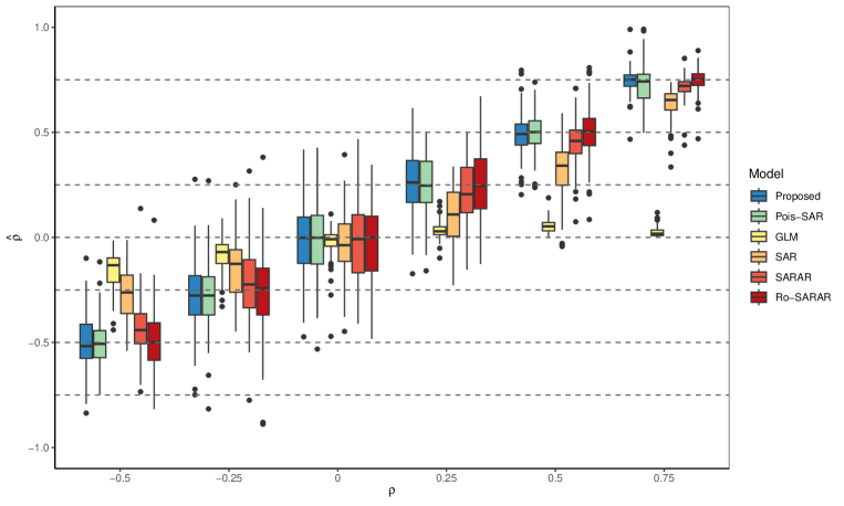
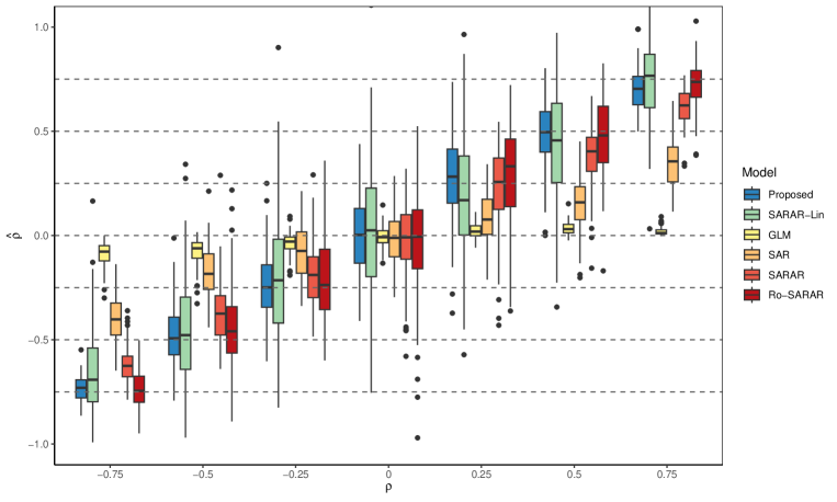
iii) Pois-SAR: Poisson SAR with logit link proposed by Lambert et al. (2010) and estimated with the sppois package (Macfarlane, 2024), iv) SAR: Maximum likelihood SAR model with normal distribution assumption for (Anselin, 1988), v) SARAR: maximum likelihood SARAR model with normal distribution assumption for (Anselin, 1988) and, vi) Ro-SARAR: Heteroscedasticity-robust SARAR model proposed in Arraiz et al. (2010) with normal distribution assumption for . The SAR, SARAR, and Ro-SARAR models were estimated using the spatialreg package (Bivand et al., 2021). Figure 1 shows the estimator of the value of for the six models when the value of . The value of estimated by the GLM in Equation (17) is the one shown for the GLM model. It is observed that the proposed model captures well the value of the parameter , with a performance similar to the Pois-SAR model, except when where the improvement of the proposed model is very noticeable. The SARAR-robust model presents a very good performance; this is explained by the approximation of the Poisson distribution to the normal distribution. The SAR and SARAR models that assume homoscedasticity estimate the parameter very poorly because although the Poisson approximates the normal well, its variance is heterogeneous and therefore, it does not meet the assumption of homoscedasticity. It is also highlighted in Figure 1 that the estimator obtained by GLM with the variable does not approach the true value of . Furthermore, the variance of the estimates of increases as gets closer to zero, except when the estimator is obtained by the usual GLM when the bias is greater.
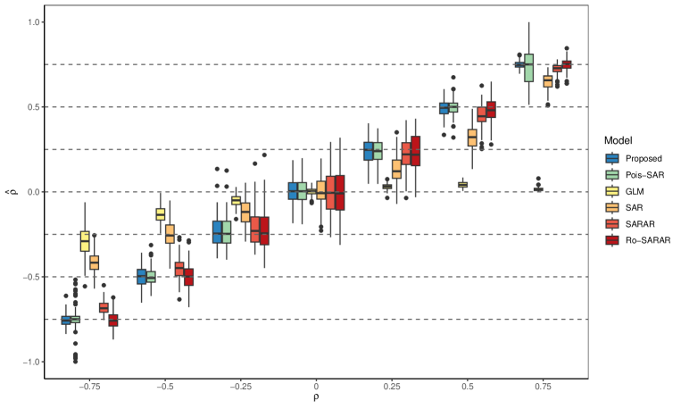
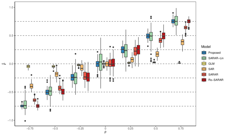
When looking at Figure 2, which is analogous to Figure 1 but with , it can be seen that the estimators now have lower variance, showing the consistency of the proposed methodology, theoretically analyzed in Theorem 1. The Pois-SAR model has a similar performance to the proposed model, except for values of , where it is very bad. The GLM here does obtain non-comparable values for the estimator. The homoscedastic normal models present a moderate performance, except when . The only model that captures the value of well is the robust SARAR, showing that in these scenarios it is indeed robust both to variance and to misspecification of the response variable. It is worth noting that the Ro-SARAR model is better than the Pois-SAR model when , although it is also rare to find real examples with very close to 1 (Arbia, 2016).
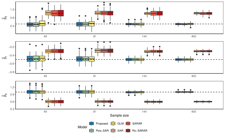
Figure 3 shows the estimators of for each of the models fitted in the simulation and also when . It is observed that the three models where the response variable is assumed to be Poisson (Proposed, Pois-SAR, and the GLM) are very similar, which shows the Corollary 3. The normal models do present a noticeable bias for each component of , something that has already been explored in Dobson and Barnett (2018).
The estimators of for each of the models when are shown in Figure 4. For , it is observed that the proposed model is the only one that is unbiased for all values of , since the Pois-SAR model is biased for . This is explained because the algorithm used in the sppois library (Macfarlane, 2024) assumes that all values of are independent, which generates biases when reaches infinity, as demonstrated in Liang and Zeger (1986). This behavior is very similar to that of the estimator given by the usual GLM. Furthermore, the estimator proposed in this paper presents a lower variance than the Pois-SAR model when the latter is unbiased, as demonstrated in Corollary 3. If the values of and are also analyzed, the Pois-SAR model and the proposed model are unbiased, but the proposed one has lower variance in all scenarios. As for the normal models, these have a very significant bias and larger variance than the proposed model for each . The proposed model also shows consistency, since the variance decreases as the sample number increases.
This shows that the methodology proposed in this work works better than methodologies with a normal distribution assumption when the response variable is Poisson, and equally and better than methodologies with a Poisson distribution assumption with independence in the observations.
3.2 Gamma Distribution
A simulation study was performed, with generated from a gamma distribution on a regular grid, following these steps:
and the following models will be fitted: i) Proposed: model given in Equation (1), ii) GLM: usual generalized linear model with linear predictor given by:
| (18) |
iii) SARAR-Lin: SARAR with assumed as normal proposed in Arraiz et al. (2010), iv) SAR: SAR model, v) SARAR: maximum likelihood SARAR model with normal distribution assumption for (Anselin, 1988), and vi) Ro-SARAR: Heteroscedasticity-robust SARAR model proposed in Arraiz et al. (2010) with normal distribution assumption for . The SARAR-Lin, SAR, SARAR and Ro-SARAR models were estimated using the spatialreg package (Bivand et al., 2021).
Figure 5 shows the estimator of the value of for the six models when the value of . The value of estimated by the GLM in Equation (18) is the one shown for the GLM model. It is observed that the proposed model captures well the value of the parameter , with a performance similar to the Ro-SARAR model, except when where the proposed model has a negative bias. The SARAR-robust model presents a very good performance, this is explained by the approximation of the Gamma distribution to a log-normal one. The SAR and SARAR models that assume homoscedasticity estimate the parameter very poorly because although the Gamma approximates well to the log-normal, its variance is heterogeneous and therefore, it does not meet the assumption of homoscedasticity.
When looking at Figure 6, which is analogous to Figure 5 but with , it can be seen that the estimators now have lower variance, showing the consistency of the proposed methodology, theoretically analyzed in Theorem 1. The behavior is very similar to that observed in , although the Ro-SARAR model and the proposed one are very similar in all values of . It is also highlighted in Figures 5 and 6 that the estimator obtained by GLM with the variable does not approach the true value of . The SARAR-Lin model estimates the parameter poorly in all the values obtained in the simulation. Regarding the bias of obtained by the proposed method, it decreases with the sample size if the figures 9 and 6 are compared, which is explained by Theorem 1.
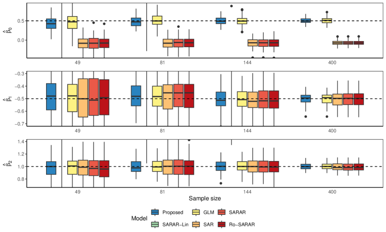
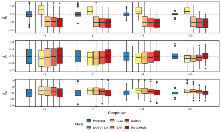
Figure 7 shows the estimators of for each fitted model in the simulation and also when . It can be observed that in the proposed model and the GLM, the estimator is very similar, which shows Corollary 3. Normal models present a noticeable bias for the component, and they acceptably estimate both and . The SARAR-Lin model presents a very large bias and that is why it does not appear in the figure. This shows that assuming normality in does not capture the effects of the variables in any way, and ot would generate very erratic conclusions about the model.
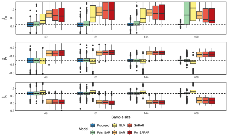
The estimators of for each model when are shown in Figure 8. For , it is observed that the proposed model is the only one that is unbiased for all values of . The GLM model is biased for almost all the scenarios presented because the GLM assumes that all values of are independent, which generates biases when reaches infinity, as shown in Liang and Zeger (1986). If the values of and are also analyzed, the Ro-SARAR and the proposed one are unbiased, but the proposed one has lower or equal variance in all scenarios than Ro-SARAR model. As for the other normal models, these have a very significant bias and larger variance than the proposed model for each . The proposed model also shows consistency, since the variance decreases as the sample number increases.
This shows that the methodology proposed in this work works better than methodologies with a normal distribution assumption when the response variable is Gamma.
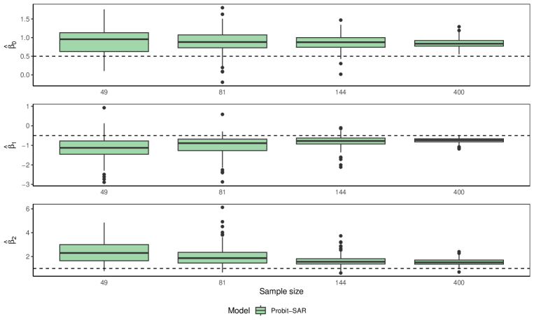
3.3 Binomial Distribution
A simulation study was performed, with generated from a binomial distribution on a regular grid, following these steps:
with selected from a discrete uniform . The following models will be fitted: i) Proposed: model given in Equation (1), ii) GLM: usual generalized linear model with linear predictor given by:
| (19) |
iii) Probit-SAR: Binomial SAR with probit link proposed by Lacombe and LeSage (2018) and estimated with the spatialprobit package (Wilhelm and Godinho de Matos, 2024) with the response variable , iv) SAR: Maximum likelihood SAR model with normal distribution assumption for (Anselin, 1988), v) SARAR: Maximum likelihood SARAR model with normal distribution assumption for (Anselin, 1988), and vi) Ro-SARAR: Heteroscedasticity-robust SARAR model proposed in Arraiz et al. (2010) with normal distribution assumption for . The SAR, SARAR, and Ro-SARAR models were estimated using the spatialreg package (Bivand et al., 2021).
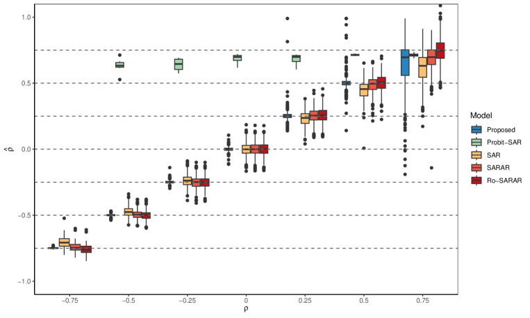
Figure 9 shows the estimator of the for the five models that estimate this component when . The estimators of the Probit-SAR model does not converge to the true value of and it has a high error rate in the execution of the spatialprobit package. Regarding the value of estimated by the GLM in Equation (19), it cannot be compared with the values of because its estimate appears outside the range (-1,1) in most scenarios. In addition, the proposed model captures well the value of the parameter in all other models, except when where the SARAR-robust model is only one that presents a good performance.
This behavior is explained because the Pearson correlation coefficient between binomial random variables is restricted by the Odds ratios as explained in the work from Lipsitz et al. (1991). Also, due to the good normal approximation for the binomial distribution when is large, the models based on normal distribution behave well with values of close to 0. The probit-SAR model presents a poor performance in its estimates, always giving values close to 0.75, which is due to the sample size of or to the incorrect specification of the normal latent variable in the methodology explained by Wilhelm and Godinho de Matos (2024).
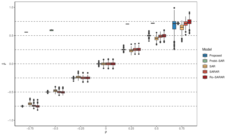
Figure 10 shows the estimator of for the five models that estimate this component when . The behavior is very similar to that observed in Figure 9, but now the variance of is very small for the proposed model, and again, for , the proposed model has a high bias and variance. The Ro-SARAR model is good in all scenarios and would be a reliable option in case of not fit the normal distribution.
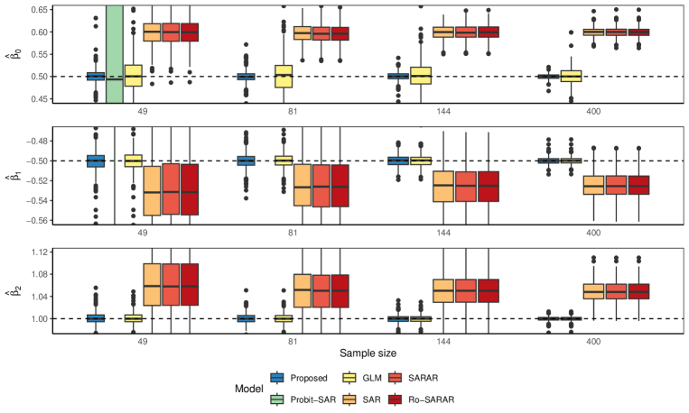
To compare the estimates between the proposed model and the Probit-SAR model, the approximation of explained in Hosmer Jr et al. (2013, pag 35) will be used. For normality-based models, will be used as explained by Train (2009, pag 24) and Hellevik (2009). Figure 11 shows the estimators of when , i.e., there is no spatial component. For the value of , the GLM and the proposed model perform well, although the inclusion of the component in Equation (19) gives more variance to the estimator under GLM. The probit-SAR model has a huge variance compared to the others when and also, for larger , it goes out of the figure, which shows that it is not useful in these scenarios where the distribution follows a logistic model. The estimators based on normal distribution present a bias given by the approximation (it is obvious that this bias happens because are comparing different models). But also its variance is larger, therefore, it is risky in spatial models to fit a model based on normal distribution when the data are proportions. For and the proposed model is the best, without a big difference with the GLM, which shows the results of the Corollary 4 and Lemma 1.
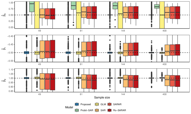
On the other hand, when , the normality-based models exhibit a lower bias, but a much larger variance than the proposed model and the GLM. The latter exhibit similar behavior and are consistent for the three components of . The Probit-SAR model presents a very high estimation variability, as observed in Figure 13. These results demonstrate the consistency and efficiency of the methodology presented in this paper, in addition to evidencing its theoretical results.
4 Application
Following the idea of Lacombe and LeSage (2018) it is of interest to explore the factors that influenced the results of the 2020 presidential election at the county level in the United States of America. One question of interest is the role played by spatial dependence. The spatial logistic model produces estimates for the spatial dependence parameter, which allows for an inference to be drawn about the presence or absence of spatial interdependence between county-level election outcomes. A second issue relates to the relative magnitude of the direct and indirect effects. The presence of such dependence is attributed to omitted variables, such as media influence, which are spatially dependent and correlated with the explanatory variables included in the model.
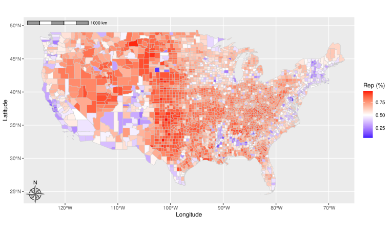
There is a large literature highlighting the importance of interdependence in the case of county-level election outcomes (Lacombe and LeSage, 2018). Correctly interpreting the estimates in terms of the magnitudes of the direct and spatial spillover effects should have important benefits for understanding issues related to election outcomes following Equation (16). The dependent variable in the empirical model of the 2020 presidential election is : Republican vote share in county . The data for the dependent variable come from the MIT election lab (MIT Election Data and Science Lab, 2024), and contains data from 3155 counties. The percentages of votes for the Republican Party in each county are shown in Figure 14. A set of county-level explanatory variables will be used to model the binary outcomes of the 2020 presidential election. These include information from the 2020 census (United States Census Bureau, 2024) on: Income: Median household income in thousands of US dollars, Civilian: the proportion of civilian employment and civilian unemployment, Unemployment: Proportion of people without employment, PercLess: Percentage of adults with less than a high school diploma, PercHigh: Percentage of adults with only a high school diploma, Birthrate: Birth rate per 100000 population, IntMigRate: International migration rate into the county per 100000 population, and Poverty: The proportion of the county’s population living in poverty (Poverty). The model proposed for the analysis is the following:
| (20) |
where is a matrix associated with the neighborhood between county and county , is the total number of votes in county , is the proportion of votes for the Republican county party and is the vector of covariates for county . The results of applying the proposed methodology are shown in Table 1, which shows the estimator, the direct, indirect, and total effect using Equation (16), and the standard error obtained by the sandwich variance for .
| Estimate | Std Error | z_value | p_value | Direct | Indirect | Total | |
|---|---|---|---|---|---|---|---|
| (Intercept) | 2.63171 | 0.61779 | 4.25990 | 0.0001 | |||
| Income | -0.02206 | 0.00486 | -4.54041 | 0.0001 | -0.02211 | 0.00235 | -0.01976 |
| Civilian | -0.49349 | 0.48033 | -1.02740 | 0.30423 | -0.49461 | 0.05255 | -0.44206 |
| Unemployment | -0.13272 | 0.01927 | -6.88817 | 0.0001 | -0.13302 | 0.01413 | -0.11889 |
| PorcLess | 0.03063 | 0.00940 | 3.25850 | 0.00112 | 0.03070 | -0.00326 | 0.02744 |
| PorcHigh | 0.03553 | 0.00661 | 5.37413 | 0.0001 | 0.03561 | -0.00378 | 0.03183 |
| BirthRate | 0.00054 | 0.00055 | 0.97813 | 0.32801 | 0.00054 | -0.00006 | 0.00048 |
| IntMigRate | -0.01460 | 0.00872 | -1.67321 | 0.09429 | -0.01463 | 0.00155 | -0.01308 |
| Poverty | -7.88634 | 1.43512 | -5.49525 | 0.0001 | -7.90424 | 0.83978 | -7.06446 |
It is worth noting that is a value that reflects a negative spatial dependence. It can be observed in the map that counties with Democratic votes are surrounded by counties with Republican votes. In addition, due to the way the model is constructed in Equation (20), more importance is given to counties with a higher population. This generates a different model than that shown by (Lacombe and LeSage, 2018) for the 2004 elections with similar variables. There, the indicator variable is used, which, as observed in the simulation results, does not capture well the autoregressive parameter of a binomial distribution, when the number of experiments, in this case, votes, per spatial unit is not constant.
Analysis of the estimates indicates that Poverty has the strongest direct effect on the share of votes for Donald Trump in 2020, with a direct impact of -7.90424, suggesting a significant negative relationship between the share of people in poverty and support for the Republican candidate. To analyze this direct impact, the odds ratio associated with a one percentage point change in poverty must be calculated, i.e., . That is, an additional one percentage point change in poverty marginally decreases the Republican vote odds ratio by 7.6%. This effect remains relevant even when considering indirect impacts, although these slightly attenuate the total effect (-7.06446). On the other hand, median household income also shows a significant impact, but of a smaller magnitude (-0.02211 for the direct impact), indicating that counties with higher incomes have a lower share of Republican votes, possibly reflecting an economic polarization in political preferences (Kulachai et al., 2023).
The percentage of adults with a high school education or less has a relevant impact. In particular, both PorcLess and PorcHigh present positive relationships with the share of Republican votes. PorcLess, with a total effect of 0.02744, and PorcHigh, with 0.03183, suggest that intermediate educational levels could be associated with preferences towards Trump, consistent with theories that link these groups with feelings of discontent or populism (Bor, 2017). These variables present negative indirect effects, indicating possible compensating influences in neighboring regions.
The Birthrate, although not significant (p=0.328), and the International Migration Rate (IntMigRate), which presents a borderline value (p=0.094), show minimal effects, suggesting that these factors are not determinants in the studied political preferences. Finally, Unemployment has a significant negative impact (direct -0.13302, p0.0001), which could indicate that areas with higher unemployment rates are less inclined towards the Republican vote. This relationship contrasts with certain political narratives suggesting that Republicans are perceived as champions of economic growth, pointing to possible complex dynamics in public perception. The Civilian variable, representing civilian employment, is not significant (p=0.304), showing a weak relationship between overall employment and political preferences in this context, perhaps already captured by the Unemployment variable (Lacombe and LeSage, 2018).
5 Conclusions
The generalized spatial autoregressive model presented in this paper offers an innovative extension to standard SAR models by incorporating the spatial dependence structure in the linear predictor for all variables whose distribution is in the exponential family. This approach allows capturing the interactions between spatial units for non-normal variables, based on the maximization of quasi-likelihood and GEE. This approach guarantees consistency and efficiency that improves the Poisson, logistic and probit models already published and used in practice. The theoretical formulation is reinforced with the derivation of the asymptotic properties of the estimators, which provides a robust framework for its practical implementation. The algorithm is developed in the R software, which will allow it to become a standard tool in the analysis of complex spatial data. The proposed GSAR proves to be more effective than other similar techniques for modeling data with spatial structure and non-normal distributions such as Poisson and Binomial. In the case of the Poisson distribution, the proposed model captures the spatial parameter more accurately, showing lower bias and variance compared to alternatives such as GLM and homoscedastic normal models (SAR and SARAR). In addition, its performance outperforms the Pois-SAR model especially for high values of , evidencing a better adjustment capacity in complex scenarios.
For data with Gamma distribution, the proposed model also showed lower bias and greater consistency compared to other approaches, including the Ro-SARAR model. This result reinforces the robustness of the methodology for heteroscedastic distributions. In the case of the Binomial distribution, the results are consistent with the previous cases: the proposed model is unbiased and consistent, outperforming conventional methods. These results highlight the applicability of the approach to spatial data with non-normal responses, positioning it as a robust and versatile tool for the analysis of spatial data.
Finally, in the analysis of the influence of the Republican vote, the proposed methodology allows for capturing spatial dependencies in the data. This application also shows the advantages of analyzing direct impacts on vote share using the results already known for GLM. In future work, non-linear behaviors in the explanatory variables should be incorporated into the model using generalized additive models (GAM).
Supplementary files
-
1.
Supplementary file 1: R files with the three simulations of this paper, the proposed methodology, and the data files.
References
- Anselin [1988] L. Anselin. Spatial Econometrics: Methods and Models. Springer Science and Business Media, 1988. Dordrecht.
- Anselin and Bera [1998] L. Anselin and A. Bera. Introduction to spatial econometrics. Handbook of applied economic statistics, 237, 1998.
- Apostol [1974] T. M. Apostol. Mathematical Analysis. Addison-Wesley, Reading, Massachusetts, 2nd edition, 1974. Theorem on absolute convergence and series multiplication.
- Arbia [2016] G. Arbia. Spatial econometrics: A rapidly evolving discipline. Econometrics, 4(1):18, 2016.
- Arraiz et al. [2010] I. Arraiz, D. M. Drukker, H. H. Kelejian, and I. R. Prucha. A spatial cliff-ord-type model with heteroskedastic innovations: Small and large sample results. Journal of Regional Science, 50(2):592–614, 2010.
- Banerjee et al. [2003] S. Banerjee, B. P. Carlin, and A. E. Gelfand. Hierarchical modeling and analysis for spatial data. Chapman and Hall/CRC, 2003.
- Bivand et al. [2021] R. Bivand, G. Millo, and G. Piras. A review of software for spatial econometrics in R. Mathematics, 9(11), 2021. 10.3390/math9111276. URL https://www.mdpi.com/2227-7390/9/11/1276.
- Bor [2017] J. Bor. Diverging life expectancies and voting patterns in the 2016 us presidential election. American journal of public health, 107(10):1560–1562, 2017.
- Casella and Berger [2002] G. Casella and R. L. Berger. Statistical Inference: Theory of Point Estimation. Springer, New York, 2nd edition, 2002. Continuity and differentiability in exponential families.
- Cepeda-Cuervo and Sicacha [2022] E. Cepeda-Cuervo and J. A. Sicacha. Spatial econometric models: A bayesian approach. Revista Colombiana de Estadística, 45(2):341–361, 2022.
- Cliff and Ord [1970] A. D. Cliff and K. Ord. Spatial autocorrelation: a review of existing and new measures with applications. Economic Geography, 46(sup1):269–292, 1970.
- Cressie [1993] N. Cressie. Statistics for spatial data. Wiley series in probability and mathematical statistics: Applied probability and statistics. John Wiley, 1993.
- De Bastiani et al. [2018] F. De Bastiani, R. A. Rigby, D. M. Stasinopoulous, A. H. Cysneiros, and M. A. Uribe-Opazo. Gaussian markov random field spatial models in gamlss. Journal of Applied Statistics, 45(1):168–186, 2018.
- Dobson and Barnett [2018] A. J. Dobson and A. G. Barnett. An introduction to generalized linear models. Chapman and Hall/CRC, 2018.
- Griffith [2009] D. Griffith. Spatially autoregressive models. In R. Kitchin and N. Thrift, editors, International Encyclopedia of Human Geography, pages 396–402. Elsevier, Oxford, 2009.
- Hardin and Hilbe [2002] J. W. Hardin and J. M. Hilbe. Generalized estimating equations. chapman and hall/CRC, 2002.
- Hellevik [2009] O. Hellevik. Linear versus logistic regression when the dependent variable is a dichotomy. Quality & Quantity, 43:59–74, 2009.
- Hosmer Jr et al. [2013] D. W. Hosmer Jr, S. Lemeshow, and R. X. Sturdivant. Applied logistic regression. John Wiley & Sons, 2013.
- Kulachai et al. [2023] W. Kulachai, U. Lerdtomornsakul, and P. Homyamyen. Factors influencing voting decision: a comprehensive literature review. Social Sciences, 12(9):469, 2023.
- Lacombe and LeSage [2018] D. J. Lacombe and J. P. LeSage. Use and interpretation of spatial autoregressive probit models. The Annals of Regional Science, 60:1–24, 2018.
- Lambert et al. [2010] D. M. Lambert, J. P. Brown, and R. J. Florax. A two-step estimator for a spatial lag model of counts: Theory, small sample performance and an application. Regional science and urban economics, 40(4):241–252, 2010.
- Lee et al. [2017] Y. Lee, L. Ronnegard, and M. Noh. Data analysis using hierarchical generalized linear models with R. CRC Press, 2017. Boca Ratón.
- LeSage and Pace [2009] J. LeSage and R. Pace. Introduction to spatial econometrics. Chapman and Hall/CRC, 2009. Boca Ratón.
- LeSage [1997] J. P. LeSage. Bayesian estimation of spatial autoregressive models. International regional science review, 20(1-2):113–129, 1997.
- Liang and Zeger [1986] K.-Y. Liang and S. L. Zeger. Longitudinal data analysis using generalized linear models. Biometrika, 73(1):13–22, 1986.
- Lipsitz et al. [1991] S. R. Lipsitz, N. M. Laird, and D. P. Harrington. Generalized estimating equations for correlated binary data: using the odds ratio as a measure of association. Biometrika, 78(1):153–160, 1991.
- Macfarlane [2024] G. Macfarlane. sppois: Spatial Autoregressive Poisson Modeling, 2024. URL https://github.com/gregmacfarlane/sppois. R package version 0.0.9000, commit 58559c9c37f9961ab79698d1725a2d4f31d01b9e.
- McCullagh [2019] P. McCullagh. Generalized linear models. Routledge, 2019.
- Mínguez et al. [2019] R. Mínguez, R. Basile, and M. Durbán. An alternative semiparametric model for spatial panel data. Statistical Methods & Applications, pages 1–40, 2019.
- MIT Election Data and Science Lab [2024] MIT Election Data and Science Lab. MIT Election Lab: Advancing the study of elections and election administration, 2024. URL https://electionlab.mit.edu/. Accessed: 2024-11-18.
- Montero et al. [2012] J. Montero, R. Mínguez, and M. Durbán. SAR models with nonparametric spatial trends. A P-spline approach. Estadística Española, 54(177):89–111, 2012.
- Nie [2006] L. Nie. Strong consistency of the maximum likelihood estimator in generalized linear and nonlinear mixed-effects models. Metrika, 63(2):123–143, 2006.
- Pan [2001] W. Pan. On the robust variance estimator in generalised estimating equations. Biometrika, 88(3):901–906, 2001.
- Plant [2018] R. E. Plant. Spatial data analysis in ecology and agriculture using R. CRC Press, 2018.
- R Core Team [2024] R Core Team. R: A Language and Environment for Statistical Computing. R Foundation for Statistical Computing, Vienna, Austria, 2024. URL http://www.R-project.org/.
- Song et al. [2022] Y. Song, Y. Su, and Z. Wang. Variable selection of spatial logistic autoregressive model with linear constraints. Entropy, 24(11):1660, 2022.
- Toloza-Delgado et al. [2021] J. Toloza-Delgado, O. Melo-Martínez, J. Azcarate-Romero, et al. Determinantes del precio de la vivienda nueva en bogotá para el año 2019: una aproximación a través de un modelo semiparamétrico de regresión espacial. Ingeniería y Ciencia, 17(34):23–52, 2021.
- Toloza-Delgado et al. [2024] J. Toloza-Delgado, O. Melo, and N. Cruz. Joint spatial modeling of mean and non-homogeneous variance combining semiparametric sar and gamlss models for hedonic prices. arXiv preprint arXiv:2409.08912, 2024.
- Train [2009] K. E. Train. Discrete choice methods with simulation. Cambridge university press, 2009.
- United States Census Bureau [2024] United States Census Bureau. 2020 Census Results, 2024. URL https://www.census.gov/programs-surveys/decennial-census/decade/2020/2020-census-results.html. Accessed: 2024-11-18.
- Van Der Vaart and Wellner [1996] W. Van Der Vaart and J. A. Wellner. Weak convergence. Springer, 1996.
- Wilhelm and Godinho de Matos [2024] S. Wilhelm and M. Godinho de Matos. spatialprobit: Spatial Probit Models, 2024. URL https://CRAN.R-project.org/package=spatialprobit. R package version 1.0.4.
- Wood [2017] S. Wood. Generalized additive models: An Introduction with R. Chapman and Hall/CRC, 2017. Boca Ratón.
- Yin et al. [2006] C. Yin, L. Zhao, and C. Wei. Asymptotic normality and strong consistency of maximum quasi-likelihood estimates in generalized linear models. Science in China Series A, 49:145–157, 2006.