Smoothing of global fields

Abstract

In the forecast diagnostic and verification community, there exists a need for smoothing methods that would work in the global domain. For limited-area domains, fast smoothing methods already exist, but the problem is that these approaches cannot be used with global fields as a global grid defined on a sphere is inherently non-equidistant and/or irregular. Another potential issue is the variability of grid point area sizes and the presence of missing data in the field, which can also be problematic to deal with for existing smoothing methods. Here, we present two new approaches for area-size-informed smoothing on a sphere. The first approach is based on k-d trees, and the second one is based on overlap detection. While each has its strengths and weaknesses, both are potentially fast enough to make the smoothing of high-resolution global fields feasible, as demonstrated by the smoothing of an operational global high-resolution precipitation forecast from the Integrated Forecasting System of the European Centre for Medium-Range Weather Forecasts. Both approaches can also handle missing data in an appropriate manner and can also be used in non-rectangularly-shaped limited-area domains defined on non-equidistant and/or irregular grids.

Keywords smoothing  $\cdot$ global domain  $\cdot$ forecast verification  $\cdot$ global forecasting  $\cdot$ spatial verification

1 Introduction

In the forecast diagnostic and verification community, there exists a need for smoothing methods that would work in the global domain. For example, the Fraction Skill Score [FSS, Roberts and Lean, 2008, Roberts, 2008], a widely used verification metric, is based on the smoothing (using a constant value smoothing kernel, aka the neighborhood) of thresholded fields. Conceptually, employing the FSS or one of its many derivatives and other similarly defined scores [e.g., Zacharov and Rezacova, 2009, Schwartz et al., 2010, Duc et al., 2013, Bouallègue et al., 2013, Dey et al., 2014, 2016, Ma et al., 2018, Woodhams et al., 2018, Skok and Roberts, 2018, Skok and Hladnik, 2018, Skok, 2022, Necker et al., 2024, Gainford et al., 2024] in spherical geometry poses no inherent issues; however, challenges emerge due to the increased computational complexity of smoothing, which is computationally the most expensive part of the score’s calculation [Skok and Lledó, 2024]. Namely, in a regular and equidistant grid, the smoothing can be done very efficiently using either the summed-fields approach [Faggian et al., 2015] with time complexity $O(n)$ or by using the Fast-Fourier-Transform-based convolution [Smith, 1999] with time complexity $O(n\log(n))$, with $n$ being the number of points in a field. The problem is that these approaches cannot be used on a sphere due to the grid being inherently non-equidistant and/or irregular. Using the so-called explicit summation for smoothing is still possible but becomes prohibitively expensive for global high-resolution-model fields consisting of millions of points due to its time complexity of $O(n^{2})$.

Another example are the object-based diagnostic and verification methods, where smoothing of the input fields is frequently performed before identifying the objects. This can merge the objects that lie very close to one another, make the shapes and outlines of the identified objects less ragged and more similar to how a human would do it, and filter out the very small objects that are caused by the possible presence of noise in the fields.

Another potential issue for the smoothing is the variability of grid point area sizes. Namely, in a global domain, the area size represented by each grid point is usually not the same for all grid points. If the smoothing would be done in a way that would not account for this, the spatial integral of the field could change considerably as a result of the smoothing. For example, the smoothing of a precipitation field could cause the total volume of precipitation in the domain to increase or decrease. To alleviate this issue, the smoothing method needs to be area-size informed.

Here, we present two new approaches for area-size-informed smoothing on a sphere. The first approach is based on k-d trees, while the second is based on overlap detection. Both are potentially fast enough to make the smoothing of high-resolution global fields feasible, but each has its strengths and weaknesses.

2 Area-size-informed smoothing

The area-size-informed smoothed value at grid point $i$ can be calculated as

$$f^{\prime}_{i}(R)=\frac{\sum\limits_{j\in\mathbb{K}_{i}(R)}f_{j}a_{j}}{\sum\limits_{j\in\mathbb{K}_{i}(R)}a_{j}},$$ (1)

where $f_{j}$ is the field value at point $j$, $a_{j}$ the area size representative for point $j$, and $\mathbb{K}_{i}(R)$ the subset of all points around point $i$, for which the great circle distance (along the spherically curved surface of the planet) to point $i$ is less than $R$. In other words, the smoothed value represents the area-size-weighted average value of points located inside a spherical-cap-shaped smoothing kernel centered on the selected point. The radius of the smoothing kernel can also be called a smoothing radius.

Fig.1 showcases an example of area-size-informed smoothing in the case of an irregular grid in two dimensions. Since the grid is irregular, the area size of points, denoted by the corresponding Voronoi cells, differ. In this case, the subset of points inside the smoothing kernel, denoted as $\mathbb{K}_{i}(R)$ in Eq.1, is shown by the gray color, while the rest of the points are white.

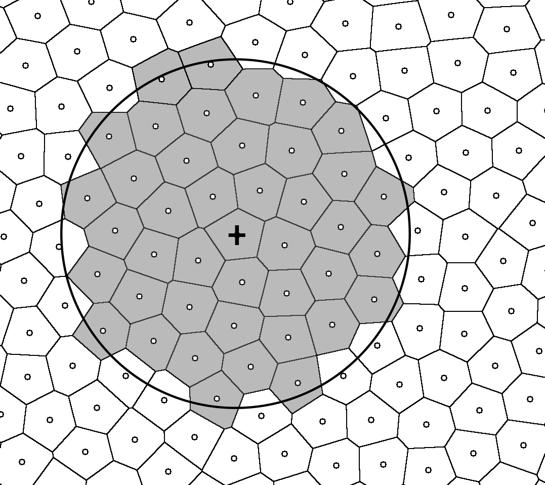
Figure 1: A visualization showcasing the area-size-informed smoothing methodology in two-dimensions. The small circles denote the grid points, while the polygons represent the corresponding Voronoi cells (defined as the region that is closest to the corresponding grid point). The large circle represents the smoothing kernel around the point denoted by a + sign, while the Voronoi cells of points inside the kernel are colored in gray.

Fig.2 shows some examples of smoothed fields of forecasted precipitation produced by the high-resolution deterministic Integrated Forecasting System [IFS, ECMWF, 2023a, b] of the European Centre for Medium-Range Weather Forecasts (ECMWF). The IFS model uses an octahedral reduced Gaussian grid O1280 [Malardel et al., 2016], which consists of around 6.5 million grid points. The area size of the points in the O1280 grid varies substantially from 18 km² (close to the poles) to 93 km² (at approximately 75º latitude).

Due to the spherical periodicity of the global domain, the smoothing kernel with $R\approx 20\,000$ km will cover the whole surface of the Earth (i.e., in this case, $\mathbb{K}_{i}(R)$ is guaranteed to contain all the grid points), resulting in the smoothed value being the same everywhere - the so-called asymptotic smoothing value. Thus, as the smoothing kernel becomes larger, the field will become less variable, with the smoothed values being ever closer to the asymptotic value. For example, Fig2i shows an example with the smoothing kernel radius $10\,000$ km, which covers about half the Earth’s surface, with the variability of the smoothed value being very low.

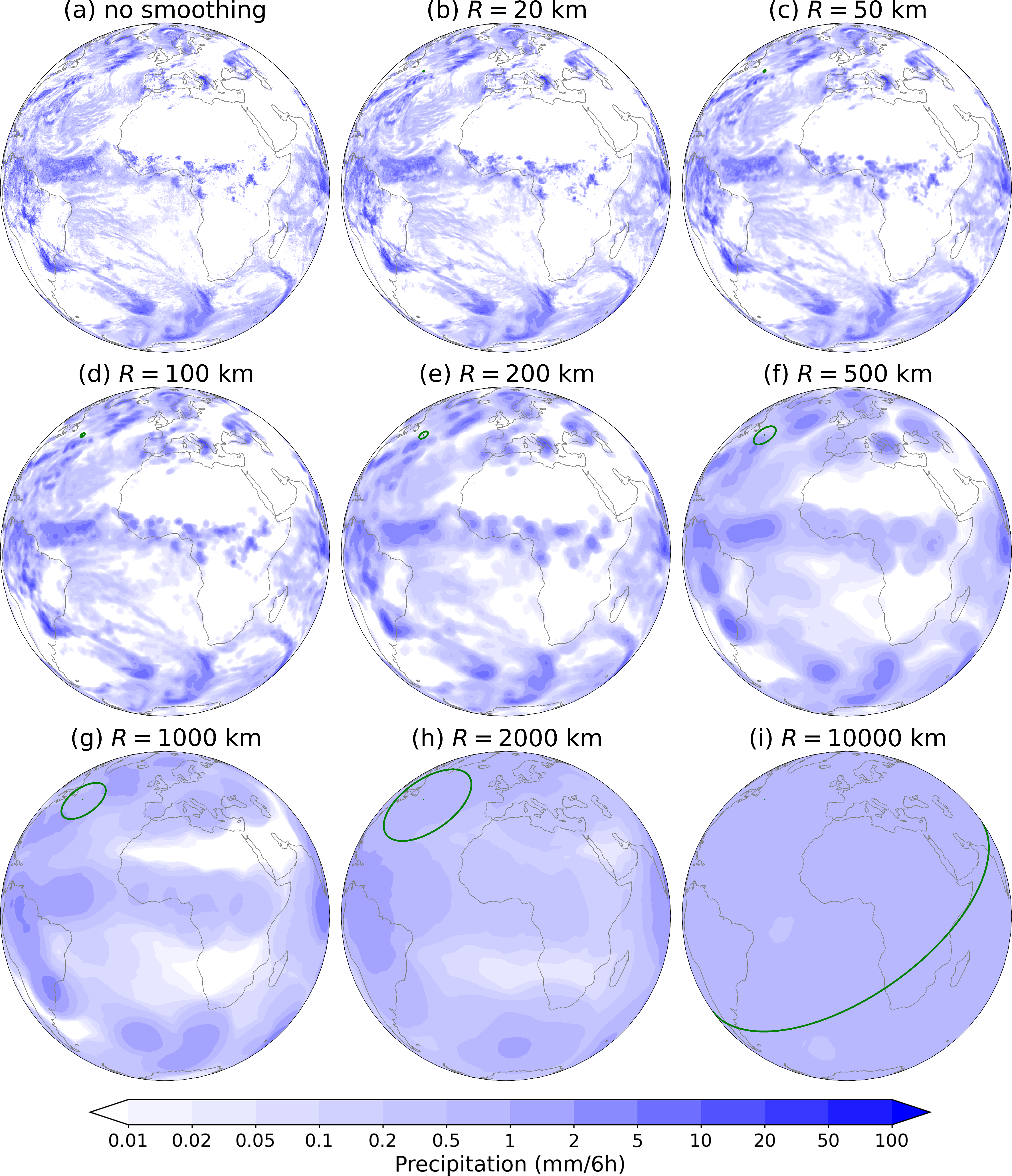
Figure 2: Visualization of smoothed fields of forecasts of 6-hourly accumulations of precipitation in the period 00-06 UTC for 11 October 2022 by the IFS model (the forecast was initialized at 00 UTC on the same day). (a) the original non-smoothed field, (b-i) the smoothed fields using a smoothing kernel radius ($R$) ranging from 20 to $10\,000$ km. The green circle indicates the size of the smoothing kernel.

To calculate the smoothed value via Eq.1, the two sums over the points located inside the smoothing kernel need to be performed. The so-called linear search approach is the most straightforward way to identify these points. In this case, a test is performed for each point in the domain by calculating its distance from the point at the center of the smoothing kernel and comparing it to the size of the smoothing kernel radius, thereby identifying the ones that satisfy this criterion.

Under the assumption that the Earth is spherical, the Great Circle Distance (GCD) between the two points can be calculated using the latitude/longitude coordinates of both points by utilizing the Haversine formula [Markou and Kassomenos, 2010]. However, using this approach, which requires the evaluation of multiple trigonometric expressions, turns out to be computationally slow.

Alternatively, the grid points can be projected from the model’s native two-dimensional spherical coordinate system into a three-dimensional Euclidean space, where all the grid points are located on the surface of a sphere. In this new coordinate system, the Euclidian distance between two points on the Earth’s surface is the so-called tunnel distance (TD), representing a straight line between the two points that goes through the sphere’s interior. The GCD can be easily converted to the TD or vice versa, using the relation

$$TD=2r_{E}\sin\left(\frac{GCD}{2r_{E}}\right)$$ (2)

or its inverse, where $r_{E}$ is the Earth’s radius. Since a larger GCD will always correspond to a larger TD and vice versa, searching for the points inside a specified search radius defined by TD in the three-dimensional space will yield the same results as using the corresponding value of GCD utilizing the Haversine formula in the model’s native two-dimensional spherical coordinate system.

Thus, for a specific value of GCD, the corresponding value of TD can be obtained via Equation 2, and used as a search radius in the three-dimensional Euclidean space. The square of the distance between the two points in a three-dimensional Euclidean space is defined as $d^{2}(i,j)=(x_{i}-x_{j})^{2}+(y_{i}-y_{j})^{2}+(z_{i}-z_{j})^{2}$, and its calculation does not require the costly evaluation of trigonometric functions. Moreover, the square of the distance can be directly compared with the precalculated square of the TD-defined search radius, thus avoiding the costly square root operation. This is why searching for the points inside the search radius in the three-dimensional Euclidean space is markedly faster than the Haversine-formula-based approach (in our case, testing showed it was approximately 50 times faster).

Nevertheless, even with the projection into the three-dimensional Euclidean space, the smoothing via the linear search approach is slow. Namely, if the number of grid points in the field is $n$, and at each point, the distance to all the other points needs to be calculated, the time complexity is $O(n^{2})$. This makes the linear-search-based approach prohibitively expensive for use with current state-of-the-art operational high-resolution models, which typically use grids with millions of points.

For example, the smoothing of a precipitation field from the IFS model shown in Fig.2a, using a 1000 km smoothing kernel radius, takes about 11 hours on an AMD Ryzen Threadripper PRO 5975WX processor when utilizing a single core. The approach can be relatively effectively parallelized in a shared-memory setup using multiple cores to parallelize the loop over all the points. Thus, using the OpenMP programming interface and utilizing ten cores instead of just one reduced the computation time from 11 hours to about 1.2 hours. However, even with the parallelization, the approach is still too slow for operational use in a typical verification setting, as the model’s performance is usually evaluated over a large set of cases represented by a sequence of fields from a longer time period or a wide array of weather situations. Thus, a clear need exists for smoothing approaches that are considerably faster.

3 K-d-tree-based area-size-informed smoothing

This approach requires the points first to be projected to the three-dimensional Euclidian space in the same manner as described for the linear-search-based approach. Same as before, the search radius in terms of TD can be calculated from GCD-defined smoothing kernel radius using Equation 2 and then used for the search in the three-dimensional Euclidean space.

Identification of points that lie inside the search radius can be sped up considerably by the use of a k-d tree [short for a k-dimensional tree, Bentley, 1975, Friedman et al., 1977, Bentley, 1979]. A k-d tree is a multidimensional binary search tree constructed for each input field by iteratively bisecting the search space into two sub-regions, each containing about half of the nonzero points of the parent region [Skok, 2023].

The so-called balanced k-d tree is constructed by first performing a partial sort of all the points according to the value of the first coordinate and then selecting the point in the middle for the first node (also called the root node), which splits the tree into two branches, each containing about half the remaining points. For each branch, the process is repeated by partially sorting the points by the second coordinate and again selecting the middle point as the node, which further splits the remaining points into two sub-branches. The process is then repeated for the third coordinate, then again for the first coordinate (in case the space is three-dimensional), and so on until all the points have been assigned to the k-d tree as nodes.

The time complexity of a balanced tree construction is $O(n\log(n))$ [Friedman et al., 1977, Brown, 2015]. For example, constructing a balanced k-d tree for about 6.5 million points of the IFS model grid took about 2.5 seconds. Note that if multiple fields that use the same grid need to be smoothed, the tree can be constructed only once and kept in memory or saved to the disk to be reused later. Once it is needed again, it can be simply loaded from the disk, which is an operation with time complexity $O(n)$.

Once the tree is constructed, the identification of points that lie inside a prescribed search radius can be performed by traversing the tree starting from the root node and moving outwards by evaluating a query at each split and backtracking to check the neighboring branches if necessary. The search can be done in $O(\log(n)+k)$ expected time, where $k$ is the typical number of points in the search region [Bentley, 1979], as opposed to $O(n)$ for the linear-search-based approach.

For all but the smallest smoothing kernels $k\gg\log(n)$, thus the time complexity can be approximated as $O(k)$. Since producing the smoothed field requires the search to be performed for all points, the expected time complexity of the smoothing using the k-d-tree-based approach is $O(nk)$ as opposed to $O(n^{2})$ for the linear-search-based approach. This means that, for small smoothing kernels, the k-d-tree-based approach will be much faster, but for large kernels, when $k$ becomes comparable to $n$, the benefit will vanish.

Fortunately, the speed of the calculation can be improved further by embedding the so-called Bounding Box (BB) information on each tree node. The BB information consists of the maximum and minimal values of the coordinates of all the points on all subbranches of a node. This information defines the extent of a multidimensional rectangular bounding box that is guaranteed to contain all the points in a specific branch. Adding BB information to the tree is trivial and very cheap since a single iterative loop over all the tree nodes is required to determine and add this data - the time complexity of this is $O(n)$, and thus the cost is almost negligible.

Once the BB data is available, it can be utilized to skip the branches that are guaranteed to fall completely outside the sphere defined by the search radius. This can be done by first determining which corner of the BB is the closest to the center of the search radius sphere. Next, if the distance of this corner to the center of the search radius sphere is larger than the search radius, then all the points in the node’s subbranches are guaranteed to be located outside the sphere, meaning this branch can be ignored entirely, thus reducing the computational load.

The BB information can also be used to identify the branches guaranteed to be fully located inside the search radius sphere. This can be done by first determining which corner of the BB is the furthest away from the center of the search sphere. Next, if the distance of this corner to the center of the search sphere is smaller than the search radius, all the points in the node’s subbranches are guaranteed to be located inside the sphere. This means that all the points in this branch can simply be added to the list of points known to be located inside the search sphere without the need to do any more checks and distance evaluations, thus reducing the computational load.

However, although the above-mentioned BB-information-based improvements do make the search markedly faster, the time complexity of the smoothing approach remains $O(nk)$, as in the end, the sums in Eq.1 still need to be performed over all the points inside the search radius sphere.

Crucially, the speed of the k-d-tree-based smoothing can be further improved by realizing that besides the BB information, additional data relevant to the smoothing can be embedded into the tree. Namely, one can precalculate the partial sums of $f_{i}a_{i}$ and $a_{i}$ terms (from Equation 1) of all the points in the node’s subbranches and add this data to each node. Similarly to adding BB information to the tree, adding the partial sums data is very cheap as it requires a single iterative loop over all the tree nodes (the time complexity is again only $O(n)$).

For branches that are fully located inside the search sphere (as mentioned above, this can be determined using the BB data), the partial sum information of a node can be used to account for all points in the whole branch without the need to dive deeper into it. Such branches, which happen to be located near the middle of the search sphere, far away from its border, can contain a large number of points, and thus, the reduction of computational cost can be potentially large, as one node can provide the sum information for many points.

This is not true for branches with points near the border region of the search sphere, as there the algorithm needs to dive very deep into the tree to accurately determine which points lie inside or outside of the search region. Thus, the main part of the remaining computation cost can be attributed to the evaluation of points located near the search sphere’s border region. Since the number of the points in the border regions is roughly proportional to $\sqrt{k}$, the time complexity of the smoothing reduces to approximately $O(n\sqrt{k})$, which is a huge improvement over $O(nk)$. If the spatial density of points is roughly constant, $\sqrt{k}$ is approximately proportional to $R$, with $R$ being the smoothing kernel radius, and the time complexity is approximately $O(nR)$.

For example, as already mentioned, the linear-search-based smoothing of the IFS precipitation field shown in Fig.2a, for a 1000 km smoothing kernel radius, takes about 11 hours on a single core, with the calculation time being similar also for other kernel sizes. In comparison, the k-d-tree-based approach takes only eight minutes on a single core and about one minute if ten cores are used in parallel. As expected, the smoothing calculation is faster if a smaller smoothing kernel is used. For example, using $R=100$ km, the calculation takes 34 s on a single core, which reduces to 4.5 s if ten cores are used in parallel. On the other hand, for very large smoothing kernels, the k-d-tree-based approach is still markedly faster than the linear-search-based approach, but the difference is not as large as for the smaller kernels. For example, for a kernel with $R=10\,000$ km, the k-d-tree-based calculation took about 70 minutes on a single core and about 12 minutes if ten cores were used in parallel.

4 Overlap-detection-based area-size-informed smoothing

While the k-d-tree-based smoothing is markedly faster than the linear-search-based approach and makes the smoothing of high-resolution fields potentially feasible, it is still relatively slow for very large smoothing kernels, which can be problematic if many fields need to be smoothed. Thus, it makes sense to try to come up with a different approach that would be even faster.

The alternative approach is based on identifying and then using the information on the overlap of the smoothing kernels centered at nearby points to increase the speed of the smoothing calculation. Fig.3 is similar to Fig.1 but also shows the smoothing kernel for a second point located to the right of the original point. The Voronoi cells with points inside the two kernels are colored with different shades of grey, according to the point being located inside both kernels or only one.

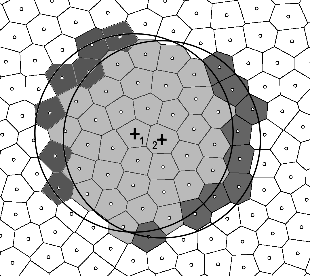
Figure 3: Same as Fig.1, but also showing the smoothing kernel for a second point located right of the original point (the points are marked with + signs and 1 and 2). The Voronoi cells of points located inside both kernels are shown with a light shade of gray. The darker shades of gray indicate the points that are located inside only one kernel

Let us assume that for the first point, the values of two sums from Eq.1 (i.e., $\sum f_{j}a_{j}$ and $\sum a_{j}$) are known. The equivalent sums for the second point can be obtained by subtracting the $f_{k}a_{k}$ or $a_{k}$ terms corresponding to the points that are located in the smoothing kernel of the first point but not the second (indicated by the dark gray shading on the left side in Fig.3), and adding the terms corresponding to the points that are located in the kernel of the second point but not the first (indicated by the dark gray shading on the right side in Fig.3). This can then be repeated for the next neighboring point, and so on.

This means that the total sums (over all the points inside the smoothing kernel) must be calculated only for the first point (which can be randomly chosen). For all the next points, the values of the sums can be obtained with the help of the nearby points for which the values of the sums are already known by subtracting and adding the appropriate terms with respect to the overlap of the two smoothing kernels. If the two points are neighbors, the number of terms that need to be subtracted and added can be approximated by the number of points that compromise the border of the smoothing kernel area - which is approximately proportional to $\sqrt{k}$.

Evaluating the overlap of the smoothing kernels of nearby points and determining which terms need to be subtracted or added can be done using the linear-search-based approach. That is, for a pair of nearby points, denoted by A (for which the values of the full sums are already known) and B, the distances from these points to all other points need to be calculated. Next, if a distance from some point P to A is smaller than the smoothing kernel radius, and at the same time, the P to B distance is larger than the smoothing kernel radius, then the terms concerning point P need to be subtracted from the values of sums for A (or added if vice versa is true) to obtain the sums for B.

For the smoothing to be performed, the only information that is needed at each point is which previously calculated point is used as a reference and the list of points that need to be added and subtracted.

Determining the reference points can be performed in a simple manner. First, from the list of all points, randomly select the initial point - this point does not have a reference point since it is the first one. Secondly, select its nearest neighbor as the second point and set the first point as its reference. Third, from the list of all remaining unassigned points, identify the nearest neighbor of the second point and use it as a third point. Fourth, from the list of all the points that have already been assigned (in this case, these are only the first and second points), identify the nearest neighbor and use it as a reference for the third point. Then, repeat steps three and four until all the points have been assigned.

Alternatively, the fourth step could be to always use the point assigned in the previous step as a reference. However, this has some downsides. Namely, the procedure is iterative, with each addition and subtraction incurring a small numerical rounding error. In a field consisting of millions of points, the numerical error could potentially accumulate (especially if a large smoothing kernel is used, as in such cases, the data from hundreds of points might need to be subtracted or added at each step). By allowing other than the point assigned in the previous step to be used as a reference, the accumulated numerical error is significantly reduced. There is also a second benefit, namely that the nearest-neighbor search can identify the reference point that is closer and thereby has better overlap of the smoothing kernel than the previously assigned point.

Fig.4 shows the number of iterative steps needed to reach a certain point in the IFS model grid (which consists of about 6.5 million points). As can be observed, the median value is about $19\,000$ steps, meaning that the number of the required steps is in the tens of thousands, not millions, and thus the numerical error remains limited.

For example, for the IFS forecast examples, shown in Fig.2, the differences between the linear-search and the overlap-detection-based approaches are smaller than $0.01$ mm/6h at all grid points, for all tested smoothing kernel radiuses ranging from 20 to $10\,000$ km. There are also additional mitigation approaches that can be implemented to further reduce the numerical error - for example, by periodically requiring the explicit calculation of the full sums (over all the points inside the smoothing kernel) each time the number of iterative steps increases by a certain threshold (e.g., $10\,000$ steps).

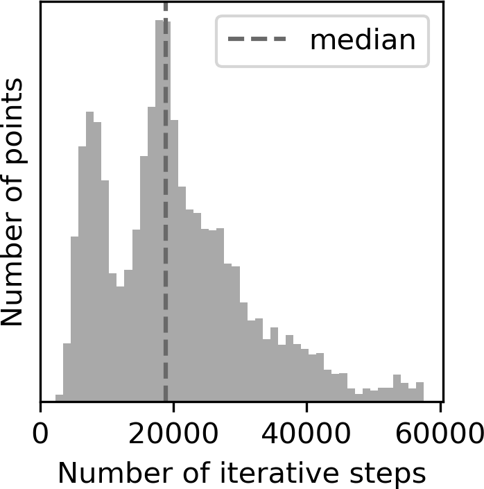
Figure 4: Histogram, showing the number of iterative steps needed to reach a specific point for the IFS model grid when using the overlap-detection-based approach. The grid consists of about 6.5 million points.

Generating the smoothing data that describes the terms that need to be added or subtracted at each point is relatively slow, but luckily, it only needs to be done once for a particular smoothing kernel size as it can be saved to disk and then simply loaded into memory whenever needed. For example, generating the smoothing data for the IFS grid for 16 different smoothing kernel sizes ($R$ ranging from 10 km to $20\,000$ km) took about 23 hours when utilizing ten cores.

The smoothing data can take up a lot of space, especially for large smoothing kernels. For example, the data for smoothing a field defined on the IFS grid takes up about 1.2 GB at $R=100$ km, 12 GB at $R=1000$ km, and 70 GB at $R=10\,000$ km (Fig.5). At $R>10\,000$ km, when the kernel becomes larger than half the Earth’s surface area, the amount of data starts to decrease as the length of the border of the smoothing kernel becomes smaller with increasing $R$ due to the spherical geometry of the global domain.

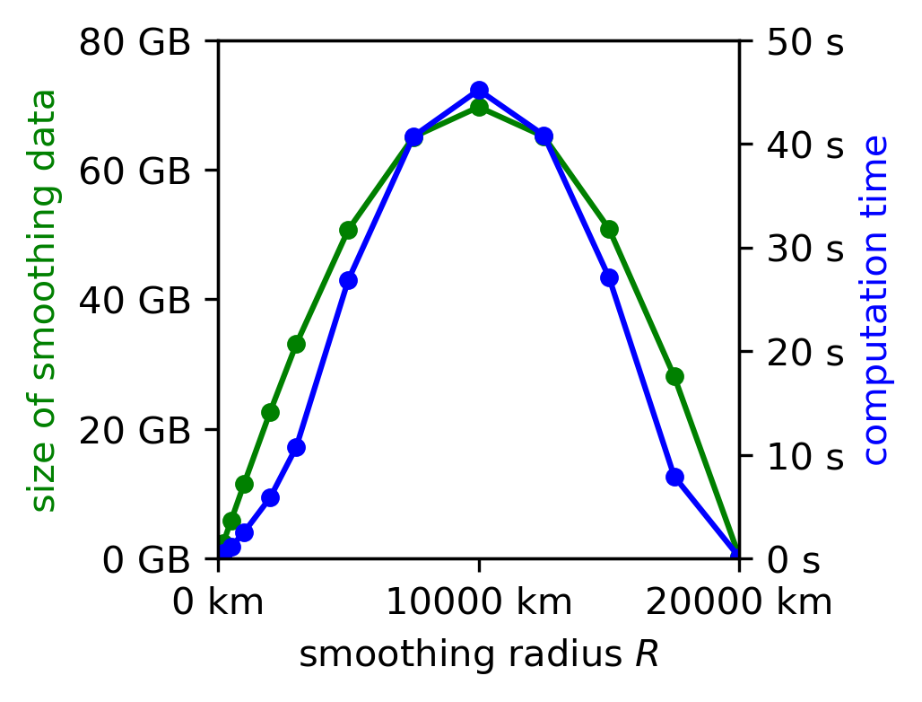
Figure 5: Size of the smoothing data (green) and computation time (blue) for the smoothing of a field defined on the IFS grid with respect to smoothing kernel radius $R$ using the overlap-detection-based approach. The computation time reflects the time needed on a computer with an AMD Ryzen Threadripper PRO 5975WX processor when utilizing a single core.

Since smoothing a field using an overlap-detection-based approach requires a simple loop that goes through all the smoothing data while adding or subtracting the appropriate terms, the time complexity of the smoothing calculation is proportional to the size of the smoothing data. On a single core, smoothing a field defined on the IFS grid takes about 0.3 s at $R=100$ km, 3 s at $R=1000$ km, and 45 s at $R=10\,000$ km (Fig.5). The 15-fold increase of calculation time when $R$ increases from $1000$ to $10\,000$ km is larger than one would expect, especially as the increase of the size of the smoothing data is only 6-fold. The larger-than-expected increase in computation time is likely related to performance degradation linked to large blocks of memory, which need to be reserved for the smoothing data in case of large smoothing kernels. Likely, the data is split over many RAM modules, which can, in turn, slow down the speed of the CPU accessing the data.

Nevertheless, for efficient calculation it is best if the smoothing data is kept in the memory, where it can be accessed quickly, as opposed to reading it from the disk every time. Thus, it makes sense to load the data from the disk into the memory as part of preprocessing and then use it to smooth multiple fields in a row. The large size of the smoothing data presents a potential problem as it requires the computer to have a large memory, at least in the case of large smoothing kernels that cover a substantial portion of the Earth’s surface.

The smoothing calculation can also be parallelized using a shared-memory setup. Namely, the calculation of the sums of the terms that need to be added or subtracted at each point, which represents the computationally most demanding part of the calculation, can be precalculated independently for each point and can thus be calculated in a parallel manner. For example, by using ten cores instead of one, the computation time for $R=1000$ km reduced from 3 to 0.6 s, while for $R=10\,000$ km, it reduced from 45 to 12 s. Although the decrease is not tenfold as one would hope (most likely due to the same memory access speed limitations mentioned earlier), the decrease is nevertheless substantial.

5 Limited-area domains and missing data

While the focus of this research was the development of methodologies for smoothing of global fields the approaches presented here can also be used to smooth fields defined on limited-area domains.

There already exist some efficient methods for smoothing of fields defined on limited-area domains. For example, the already mentioned summed-fields and Fast-Fourier-Transform-convolution-based approaches (see the Introduction section for details). However, the use of these two approaches is limited to regular grids, which are assumed to be defined in a rectangularly shaped domain on a plane, and they also assume equal area sizes for the grid points.

The approaches presented here do not have these limitations and can thus be used with irregular grids defined in non-rectangularly shaped domains, while the smoothed values also reflect the potential differences in area size of different grid points. Moreover, the approaches also correctly handle the spherical curvature of the planet’s surface, which can be important in the case of very large domains and for ensuring consistent size and shape of the smoothing kernel everywhere in the domain.

The smoothing calculation for a limited-area domain is done in the same way as for the global domain and is again based on Eq.1. As before, all that is needed is a list of grid points with values and corresponding latitude, longitude coordinates, and the associated area-size data. In the case of a limited-area domain, the points will come only from a specific geographic sub-region, as opposed to the whole Earth, like in the case of a global domain. Any of the two approaches, the k-d-tree-based and the overlap-detection-based, can be used to calculate the smoothed values.

Fig.6 shows an example of smoothing in a limited-area domain defined over Europe that encompasses the region 20W-40E, 30N-70N. The precipitation data is taken from the IFS forecast shown in Fig. 2 but with points outside the domain removed. Out of $6\,599\,680$ points of the full octahedral reduced Gaussian grid used by the IFS, only $217\,421$ points located inside the domain were selected and used to calculate the smoothed values. Figs.6a,b show the original and smoothed precipitation using a 200 km smoothing radius.

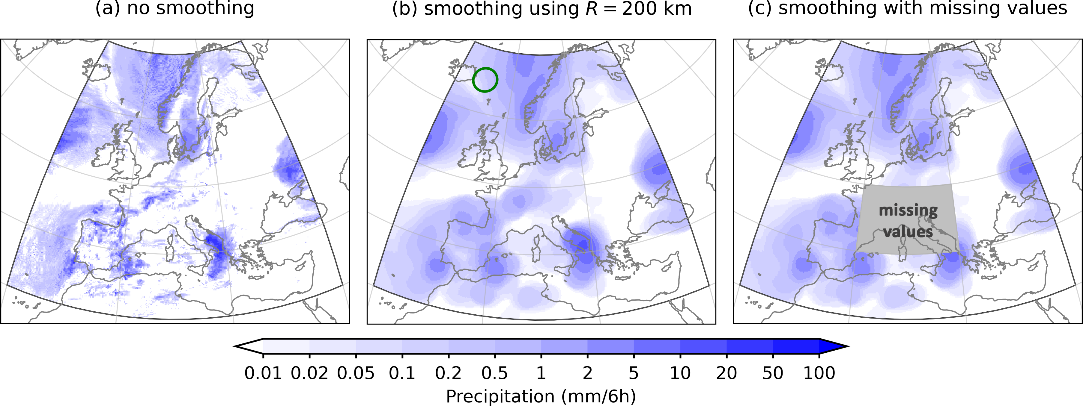
Figure 6: Smoothing in a limited-area domain centered over Europe. The precipitation data is taken from the IFS forecast shown in Fig.2. (a) the original non-smoothed precipitation field, (b) the smoothed field using a 200 km smoothing kernel radius with the size of the kernel shown with a green circle in the top left corner, (c) the smoothed field using a 200 km kernel radius in the presence of a missing data region in the middle of the domain (indicated in gray).

One noticeable feature is that the values near the domain borders do not decrease towards zero - which would happen, for example, if the smoothing method assumed the values outside the domain were zero. Moreover, although in terms of the latitude/longitude grid, the domain might be considered rectangular, it is not actually rectangular if the spherical shape of the Earth is taken into account, as the northern domain border is much shorter than the southern one.

The methodology presented here can also handle missing data (i.e., points for which the value is not defined) in an appropriate manner. Frequently, a smoothing method must make some kind of assumption regarding the values of missing data. For example, the aforementioned summed-fields and Fast-Fourier-Transform-convolution-based approaches must assume some values (e.g., zero is frequently used for precipitation) for the missing data for the calculation of the smoothed values to be successfully performed. This is problematic since it can artificially increase or decrease the values of points close to the regions with missing data (depending on which value is assumed for the missing data points).

With the methodology presented here, the missing data points can be handled appropriately by excluding them from the two sums in Eq.1. In practice, the same result can be achieved most easily by temporarily setting the area size of these points to zero before proceeding with calculating the smoothed values (this will result in the missing data points not having any influence on the smoothed values).

Fig.6c shows an example of smoothing in the presence of missing data, where a region in the center of the domain (0E-20E, 40N-50N) was assigned a missing data flag. It can be observed that the values near the missing data region do not decrease towards zero, which would happen if the smoothing method assumed the missing data had zero value.

6 Discussion and Conclusions

We present two new methodologies for smoothing fields on a sphere, one based on k-d trees and one on overlap detection. The k-d-tree-based approach requires less memory and can be done in a single step without any additional preprocessing, but is slower, especially for large smoothing kernels.

The overlap-identification-based approach requires a preprocessing step that generates the smoothing data, which needs to be calculated only once for a specific size of the smoothing kernel. Once available, this data can be used to calculate the smoothed values much faster than the k-d-tree-based approach. The large size of the smoothing data presents a potential problem as it requires the computer to have a large memory (this is only problematic if a very large smoothing kernel is used). Since the procedure is iterative, the approach can also incur a degree of numerical error, but simple mitigation strategies exist that can be implemented to address this issue.

Alternatively, similarly to how it is done for the overlap-identification-based approach, the smoothing data for the k-d-tree-based approach, which would list all the nodes that need to be summed to get the smoothed value at a certain location for a particular size of the smoothing kernel, could be precalculated and saved to the disk. This data could then be simply loaded into memory when needed and used to quickly calculate the smoothed values, similarly to how it is done for the overlap-identification-based approach. However, testing showed that the size of this data is a few times larger than for the overlap-identification-based approach, meaning that the calculation of the smoothed values would be correspondingly slower.

Both methodologies can be used when the grid is not regular, thus avoiding the need for prior interpolation into a regular grid, which can introduce additional smoothing [Konca-Kedzierska et al., 2023]. They also take into account the spherical geometry of Earth, which is important to ensure a consistent size and shape of the smoothing kernel everywhere on the planet.

The methodologies are also area-size-informed, meaning that they take into account the potentially different area sizes of the grid points. This is important since in some grids (e.g., a regular latitude/longitude grid), the difference between area sizes of points at different locations on the planet can be very large. Not accounting for this could result in negative effects, for example, the spatial integral of the field could change considerably due to the smoothing.

While the focus was on the development of methodologies for smoothing of global fields both approaches can also be used in limited-area domains. Moreover, they are both able to deal with missing data in an appropriate manner. This is important since dealing with missing values can be problematic for some smoothing methods, as they are oftentimes forced to make some kind of assumptions regarding the value of missing data, which can cause the values near the missing data region to artificially increase or decrease.

Overall, while each approach has its strengths and weaknesses, both are potentially fast enough to make the smoothing of high-resolution global fields feasible, which was the primary goal set at the beginning. The time complexity of both approaches can be approximated by $O(n\sqrt{k})$ with $k$ being the typical number of points in the smoothing kernel, which is limited by $n$ in the worst case.

Based on the methodologies presented here, we also prepared and published an easy-to-use Python software package for efficient calculation of the smoothing (please refer to the Data Availability Statement for details on how to obtain the package).

Funding

Slovenian Research And Innovation Agency (Javna agencija za znanstvenoraziskovalno in inovacijsko dejavnost RS) research core funding No. P1-0188.

Data Availability Statement

A Python software package for efficient calculation of the smoothing on the sphere is freely available on GitHub at https://github.com/skokg/Smoothing_on_Sphere.

References

- Bentley [1975] J. Bentley. Multidimensional binary search trees used for associative searching. Communications of the ACM, 18:509–517, 9 1975. ISSN 0001-0782. doi: 10.1145/361002.361007.
- Bentley [1979] J. Bentley. Multidimensional binary search trees in database applications. IEEE Transactions on Software Engineering, SE-5:333–340, 7 1979. ISSN 0098-5589. doi: 10.1109/TSE.1979.234200.
- Bouallègue et al. [2013] Z. B. Bouallègue, S. E. Theis, and C. Gebhardt. Enhancing cosmo-de ensemble forecasts by inexpensive techniques. Meteorologische Zeitschrift, 22:49–59, 2 2013. ISSN 0941-2948. doi: 10.1127/0941-2948/2013/0374.
- Brown [2015] R. A. Brown. Building a Balanced -d Tree in Time. Journal of Computer Graphics Techniques (JCGT), 4(1):50–68, mar 2015. ISSN 2331-7418. URL http://jcgt.org/published/0004/01/03/.
- Dey et al. [2014] S. R. A. Dey, G. Leoncini, N. M. Roberts, R. S. Plant, and S. Migliorini. A spatial view of ensemble spread in convection permitting ensembles. Monthly Weather Review, 142:4091–4107, 11 2014. ISSN 0027-0644. doi: 10.1175/MWR-D-14-00172.1.
- Dey et al. [2016] S. R. A. Dey, R. S. Plant, N. M. Roberts, and S. Migliorini. Assessing spatial precipitation uncertainties in a convective-scale ensemble. Quarterly Journal of the Royal Meteorological Society, 142:2935–2948, 10 2016. ISSN 0035-9009. doi: 10.1002/qj.2893.
- Duc et al. [2013] L. Duc, K. Saito, and H. Seko. Spatial-temporal fractions verification for high-resolution ensemble forecasts. Tellus A: Dynamic Meteorology and Oceanography, 65:18171, 12 2013. ISSN 1600-0870. doi: 10.3402/tellusa.v65i0.18171.
- ECMWF [2023a] ECMWF. Ifs documentation cy48r1 - part iii: Dynamics and numerical procedures. 2023a. doi: 10.21957/26F0AD3473. URL https://www.ecmwf.int/en/elibrary/81369-ifs-documentation-cy48r1-part-iii-dynamics-and-numerical-procedures.
- ECMWF [2023b] ECMWF. Ifs documentation cy48r1 - part iv: Physical processes. 2023b. doi: 10.21957/02054F0FBF. URL https://www.ecmwf.int/en/elibrary/81370-ifs-documentation-cy48r1-part-iv-physical-processes.
- Faggian et al. [2015] N. Faggian, B. Roux, P. Steinle, and B. Ebert. Fast calculation of the fractions skill score. MAUSAM, 66:457–466, 7 2015. ISSN 0252-9416. doi: 10.54302/mausam.v66i3.555.
- Friedman et al. [1977] J. H. Friedman, J. L. Bentley, and R. A. Finkel. An algorithm for finding best matches in logarithmic expected time. ACM Transactions on Mathematical Software, 3:209–226, 9 1977. ISSN 0098-3500. doi: 10.1145/355744.355745.
- Gainford et al. [2024] A. Gainford, S. L. Gray, T. H. A. Frame, A. N. Porson, and M. Milan. Improvements in the spread–skill relationship of precipitation in a convective-scale ensemble through blending. Quarterly Journal of the Royal Meteorological Society, 150:3146–3166, 7 2024. ISSN 0035-9009. doi: 10.1002/qj.4754.
- Konca-Kedzierska et al. [2023] K. Konca-Kedzierska, J. Wibig, and M. Gruszczyńska. Comparison and combination of interpolation methods for daily precipitation in poland: evaluation using the correlation coefficient and correspondence ratio. Meteorology Hydrology and Water Management, 9 2023. ISSN 2299-3835. doi: 10.26491/mhwm/171699.
- Ma et al. [2018] S. Ma, C. Chen, H. He, D. Wu, and C. Zhang. Assessing the skill of convection-allowing ensemble forecasts of precipitation by optimization of spatial-temporal neighborhoods. Atmosphere, 9:43, 1 2018. ISSN 2073-4433. doi: 10.3390/atmos9020043.
- Malardel et al. [2016] S. Malardel, N. Wedi, W. Deconinck, M. Diamantakis, C. Kuehnlein, G. Mozdzynski, M. Hamrud, and P. Smolarkiewicz. A new grid for the ifs. ECMWF Newsletter, (146):23–28, 2016. doi: 10.21957/ZWDU9U5I. URL https://www.ecmwf.int/node/17262.
- Markou and Kassomenos [2010] M. Markou and P. Kassomenos. Cluster analysis of five years of back trajectories arriving in athens, greece. Atmospheric Research, 98:438–457, 11 2010. ISSN 01698095. doi: 10.1016/j.atmosres.2010.08.006.
- Necker et al. [2024] T. Necker, L. Wolfgruber, L. Kugler, M. Weissmann, M. Dorninger, and S. Serafin. The fractions skill score for ensemble forecast verification. Quarterly Journal of the Royal Meteorological Society, 150:4457–4477, 10 2024. ISSN 0035-9009. doi: 10.1002/qj.4824.
- Roberts [2008] N. Roberts. Assessing the spatial and temporal variation in the skill of precipitation forecasts from an NWP model. Meteorological Applications, 15(1):163–169, mar 2008. ISSN 13504827. doi: 10.1002/met.57. URL https://onlinelibrary.wiley.com/doi/10.1002/met.57.
- Roberts and Lean [2008] N. M. Roberts and H. W. Lean. Scale-Selective Verification of Rainfall Accumulations from High-Resolution Forecasts of Convective Events. Monthly Weather Review, 136(1):78–97, jan 2008. ISSN 1520-0493. doi: 10.1175/2007MWR2123.1. URL http://journals.ametsoc.org/doi/10.1175/2007MWR2123.1.
- Schwartz et al. [2010] C. S. Schwartz, J. S. Kain, S. J. Weiss, M. Xue, D. R. Bright, F. Kong, K. W. Thomas, J. J. Levit, M. C. Coniglio, and M. S. Wandishin. Toward improved convection-allowing ensembles: Model physics sensitivities and optimizing probabilistic guidance with small ensemble membership. Weather and Forecasting, 25:263–280, 2 2010. ISSN 1520-0434. doi: 10.1175/2009WAF2222267.1.
- Skok [2022] G. Skok. A New Spatial Distance Metric for Verification of Precipitation. Applied Sciences, 12(8):4048, apr 2022. ISSN 2076-3417. doi: 10.3390/app12084048. URL https://www.mdpi.com/2076-3417/12/8/4048.
- Skok [2023] G. Skok. Precipitation attribution distance. Atmospheric Research, 295, 2023. ISSN 01698095. doi: 10.1016/j.atmosres.2023.106998.
- Skok and Hladnik [2018] G. Skok and V. Hladnik. Verification of gridded wind forecasts in complex alpine terrain: A new wind verification methodology based on the neighborhood approach. Monthly Weather Review, 146:63–75, 1 2018. ISSN 0027-0644. doi: 10.1175/MWR-D-16-0471.1.
- Skok and Lledó [2024] G. Skok and L. Lledó. Spatial verification of global precipitation forecasts, 2024. URL https://arxiv.org/abs/2407.20624.
- Skok and Roberts [2018] G. Skok and N. Roberts. Estimating the displacement in precipitation forecasts using the Fractions Skill Score. Quarterly Journal of the Royal Meteorological Society, 144(711):414–425, 2018. ISSN 1477870X. doi: 10.1002/qj.3212.
- Smith [1999] S. W. Smith. The Scientist and Engineer’s Guide to Digital Signal Processing. California Technical Publishing, 1999. ISBN 0-9660176-7-6.
- Woodhams et al. [2018] B. J. Woodhams, C. E. Birch, J. H. Marsham, C. L. Bain, N. M. Roberts, and D. F. A. Boyd. What is the added value of a convection-permitting model for forecasting extreme rainfall over tropical east africa? Monthly Weather Review, 146:2757–2780, 9 2018. ISSN 0027-0644. doi: 10.1175/MWR-D-17-0396.1.
- Zacharov and Rezacova [2009] P. Zacharov and D. Rezacova. Using the fractions skill score to assess the relationship between an ensemble qpf spread and skill. Atmospheric Research, 94:684–693, 12 2009. ISSN 01698095. doi: 10.1016/j.atmosres.2009.03.004.