Do anomalies break the momentum routing invariance?

Abstract

The diagrammatic computation of anomalies is usually associated with the breaking of the momentum routing invariance. This is because the momentum routing is usually chosen to fulfill the desired Ward identity. In the case of the chiral anomaly, the momentum routing is chosen in order to fulfill the gauge Ward identity and break the chiral Ward identity. Although the chiral anomaly is physical because it is associated with the pion decay into two photons, this does not necessarily mean that the momentum routing invariance is broken because the momentum routing was chosen in the computation of the anomaly. In this work, we show that if gauge invariance is assumed, the chiral and the scale anomalies are independent of the momentum routing chosen and as a result they are momentum routing invariant. Thus, it turns out that momentum routing invariance might be violated when there is a gauge anomaly.

I Introduction

Symmetries are in the main core of physics. Our current knowledge of physical laws are built based on the concept of symmetry and symmetry breaking. For instance, the form of particle interactions is determined by the symmetries of the model, Super-symmetric theories are build based on the Poincaré group and the very concept of an elementary particle, its mass and its spin are related with symmetry. Not to mention that the process of mass generation in the Standard Model of particles comes from the spontaneous symmetry breaking of a larger gauge symmetry in a smaller one. Over and above that, we desire that physical laws be unchanged under boosts and rotations, the existence of magnetic monopoles would reveal an expected symmetry of the Maxwell equations and the unbalanced asymmetry between matter and anti-matter in the universe is still an unanswered question.

Symmetries are so important for field theories that historically they were taken for granted not only at the classical level but also at the quantum one. Therefore, the name anomaly was given to a quantum breaking of a classical symmetry as it was something unusual and not desired. At the same time, regularization schemes usually break symmetries of the theory and restoring counter-terms are then required in the process of renormalization. Thus, the question whether the anomaly is indeed physical or spurious, i. e. caused by the regularization scheme, is frequently raised. For instance, Lattice regularization turns space-time discrete and this breaks Lorentz symmetry, among others like Super-symmetry and chiral symmetry [1], or cutoff regularization explicit breaks gauge symmetry and it can be constructed to maintain this symmetry and the Lorentz one [2]. However, in both cases the breaking of the symmetries is an artifact of the regularization. On the other hand, anomalies are related to physical processes and therefore can be measured. Pioneer works revealed that the chiral anomaly is related with the neutral pion decay into two photons [3]-[5] and the trace anomaly of the Quantum Electrodynamics (QED) is related to the hadronic $R$ ratio [6]. Nowadays, there are numerous applications of the anomalies like in the quantum Hall effect of Weyl semi-metals [7], chiral magnetic effects for theories with chemical potentials [8], form factors of particle processes in effective field theories [9], glueball mass spectrum [10] or even the relation of chiral anomalous processes with a quark anomalous magnetic moment [9, 11]. The application of the chiral anomaly in solid state physics is even more diverse than in particle physics. Since one of its first applications to Weyl fermions in a crystal [12], the chiral anomaly was shown to affect the magneto-transport of Weyl semimetals [13]-[16] and observations of negative magneto-resistance for different materials support the existence of this anomaly [14]-[16]. For a review on the Weyl and Dirac semimetals and the applications of the chiral anomaly in these materials see [17].

In this work, we present examples that show that the diagrammatic computation of anomalies, for a specific momentum routing, does not necessarily imply that momentum routing invariance of the Feynman diagrams is broken. In particular, we consider the examples of the chiral anomaly ( we adopt this nomenclature although it is also known as the axial anomaly, the Adler-Bardeen-Bell-Jackiw anomaly or even the triangle anomaly) for chiral abelian gauge theories and the scale anomaly for QED.

The paper is divided as follows: in section II, we present a summary of implicit regularization. In section III, we discuss some examples of momentum routing invariance of the Feynman diagrams and its relation to gauge symmetry. In section IV, we present a simple approach to compute the chiral anomaly. In section V, we present a non-trivial approach to compute the chiral anomaly for general momentum routings of the internal lines. In section VI, we compute the scale anomaly of QED for a general momentum routing and show that, as in the chiral anomaly example, the result of the anomaly is independent of the momentum routing. Finally, we present the conclusions in section VII.

II Outline of Implicit Regularization

We apply the implicit regularization scheme [18] to treat the integrals which appear in the amplitudes of the next sections. Some regularization schemes like dimension regularization [19, 20], and its extensions like dimension reduction, although widely used is a regularization scheme which is already gauge and momentum routing invariant and some of the following discussions would be trivial.

Implicit regularization is generally applied to theories with dimension specific objects, like $\gamma^{5}$ matrices and Levi-Civita symbols. Also, since it is a scheme that does not have any restriction (except for theories with non-linear propagators such as the Sine-Gordon model) and do not break symmetries of the theory, it is usually used for computation of anomalies. A recent computation for a general momentum routing concerns gravitational anomalies in two dimensions [21]. Other scenarios with Lorentz violation, like in the Bumblebee model [22], or chiral models [23] deal directly with $\gamma^{5}$ matrices and comparison with other regularization techniques is performed [22, 23, 24]. Let us make a brief review of the method in four dimensions. In this scheme, we assume that the integrals are regularized by an implicit regulator $\Lambda$ in order to allow algebraic operations within the integrands. We then use the following identity

$$\int_{k}\frac{1}{(k+p)^{2}-m^{2}}=\int_{k}\frac{1}{k^{2}-m^{2}}-\int_{k}\frac{(p^{2}+2p\cdot k)}{(k^{2}-m^{2})[(k+p)^{2}-m^{2}]},$$ (1)

where $\int_{k}\equiv\int^{\Lambda}\frac{d^{4}k}{(2\pi)^{4}}$, to separate basic divergent integrals (BDI’s) from the finite part. These BDI’s are defined as follows

$$I^{\mu_{1}\cdots\mu_{2n}}_{log}(m^{2})\equiv\int_{k}\frac{k^{\mu_{1}}\cdots k^{\mu_{2n}}}{(k^{2}-m^{2})^{2+n}}$$ (2)

and

$$I^{\mu_{1}\cdots\mu_{2n}}_{quad}(m^{2})\equiv\int_{k}\frac{k^{\mu_{1}}\cdots k^{\mu_{2n}}}{(k^{2}-m^{2})^{1+n}}.$$ (3)

The BDI’s with Lorentz indexes can be judiciously combined as differences between integrals with the same superficial degree of divergence, according to the equations below, which define surface terms :

$$\Upsilon^{\mu\nu}_{2w}=g^{\mu\nu}I_{2w}(m^{2})-2(2-w)I^{\mu\nu}_{2w}(m^{2})\equiv\upsilon_{2w}g^{\mu\nu},$$ (4)

$$\Xi^{\mu\nu\alpha\beta}_{2w}=g^{\{\mu\nu}g^{\alpha\beta\}}I_{2w}(m^{2})-4(3-w)(2-w)I^{\mu\nu\alpha\beta}_{2w}(m^{2})\equiv$$

$$\equiv\xi_{2w}(g^{\mu\nu}g^{\alpha\beta}+g^{\mu\alpha}g^{\nu\beta}+g^{\mu\beta}g^{\nu\alpha}).$$ (5)

In the expressions above, $2w$ is the degree of divergence of the integrals and we adopt the notation such that indexes $0$ and $2$ mean $log$ and $quad$, respectively. Surface terms can be conveniently written as integrals of total derivatives, as presented below

$$\upsilon_{2w}g^{\mu\nu}=\int_{k}\frac{\partial}{\partial k_{\nu}}\frac{k^{\mu}}{(k^{2}-m^{2})^{2-w}},$$

(6)

$$(\xi_{2w}-v_{2w})(g^{\mu\nu}g^{\alpha\beta}+g^{\mu\alpha}g^{\nu\beta}+g^{\mu\beta}g^{\nu\alpha})=\int_{k}\frac{\partial}{\partial k_{\nu}}\frac{2(2-w)k^{\mu}k^{\alpha}k^{\beta}}{(k^{2}-m^{2})^{3-w}}.$$ (7)

We see that equations (4)-(5) are undetermined because they are differences between divergent quantities. Each regularization scheme gives a different value for these terms. However, as physics should not depend on the scheme applied and neither on the arbitrary surface term, we leave these terms to be arbitrary until the end of the calculation and then we fix them by symmetry constraints or phenomenology [25].

Of course the same idea can be applied for any dimension of space-time and for higher loops. Equation (1) is used recursively until the divergent piece is separated from the finite one. This procedure makes the finite integrals hard to compute due to the number of $k$’s in the numerator. A simpler alternative to this approach is presented in [26], where the Feynman parametrization is applied before separating the BDI’s. However, in order to apply this simpler approach we have to assume that the integrals are momentum routing invariant in order to apply the Feynman parametrization in the divergent integral. This would compromise our proof in the examples of the next sections once that we want to show that anomalies are momentum routing invariant. Also, eq. (1) is not the only possible equation to be used since the implicit regulator was assumed to allow the use of other identities.

III Momentum Routing Invariance of Feynman diagrams

Let us consider the simple example of a 1-loop Feynman diagram of a $\phi^{4}$ scalar theory presented in figure 1. We see that there is a freedom of adding an arbitrary momentum routing $l$ in the internal line because this is also compatible with momentum conservation at the vertex. The Feynman rules lead to the following equality of integrals if we require momentum routing invariance:

$$\int\frac{d^{4}k}{(2\pi)^{4}}\frac{1}{(k^{2}-m^{2})}=\int\frac{d^{4}k}{(2\pi)^{4}}\frac{1}{[(k+l)^{2}-m^{2}]}.$$ (8)

If this 1-loop diagram is part of a scattering process, physics should not depend on the way we label the internal lines. The integral is quadratic divergent and adding a $l$ in the internal momentum routing is not simply make a shift in the integral. So, these integrals require a regularization scheme. For instance, dimensional regularization [19, 20] is a scheme that allows for shifts in the integrand even if the integral is divergent. So, the identity in eq. (8) is trivially fulfilled. We can, alternatively, assume that an implicit regulator exists and compute the integrals, as presented in section II. The regularized integrals are found in the appendix. When doing this computation a surface term appear and if we require momentum routing invariance we find out that

$$I_{quad}(m^{2}) =I_{quad}(m^{2})-l^{2}\upsilon_{0}$$

$$\Rightarrow l^{2}\upsilon_{0}=0.$$ (9)

Since the momentum routing $l$ can be any momentum, the solution is to make the arbitrary surface term $\upsilon_{0}$ equals to zero to assure momentum routing invariance and make the scattering process independent of this. The renormalization of scalar theories was performed beyond 1-loop order and it was shown that observables such as the beta function would depend on the arbitrary surface terms if we do not require momentum routing invariance [27].

Figure 1: Momentum routing invariance of a 1-loop Feynman diagram of the scalar theory $\phi^{4}$.

In abelian gauge field theories and in chiral ones, there is an additional reason that leads to momentum routing invariance. Gauge symmetry is diagrammatically related with momentum routing invariance in a regularization independent way. As an example, we can consider a two point diagram where we insert an external momentum photon leg. The gauge Ward identity is obtained by inserting the photon leg wherever is possible in the diagram [28]. In the case of a two point diagram, there is only two possibilities. After performing the simple algebra $\not{p}=\not{k}+\not{k}_{2}+\not{p}-m-(\not{k}+\not{k}_{2}-m)$, we can split both diagrams and find out that the gauge Ward identity is simply the difference between two diagrams with different momentum routing as we can see in figure 2 and algebraically as below:

$$p_{\lambda}A^{\lambda\mu\alpha}= \int_{k}Tr\left[\frac{1}{\not{k}+\not{l}-m}\not{p}\frac{1}{\not{k}+\not{l}-\not{p}-m}\gamma^{\beta}\frac{1}{\not{k}+\not{l}-\not{p}-\not{q}-m}\gamma^{\alpha}\gamma^{5}\right]+$$

$$+\int_{k}Tr\left[\frac{1}{\not{k}+\not{l}-m}\gamma^{\beta}\frac{1}{\not{k}+\not{l}-\not{q}-m}\not{p}\frac{1}{\not{k}+\not{k}_{2}-\not{p}-\not{q}-m}\gamma^{\alpha}\gamma^{5}\right]=$$

$$= \int_{k}Tr\left[\frac{1}{\not{k}+\not{l}-\not{p}-m}\gamma^{\beta}\frac{1}{\not{k}+\not{l}-\not{q}-\not{p}-m}\gamma^{\alpha}\gamma^{5}\right]$$

$$-\int_{k}Tr\left[\frac{1}{\not{k}+\not{l}-m}\gamma^{\beta}\frac{1}{\not{k}+\not{l}-\not{q}-m}\gamma^{\alpha}\gamma^{5}\right],$$ (10)

where $l$ is an arbitrary momentum routing.

So, if we require gauge symmetry, we have automatically momentum routing invariance. This proof can be generalized for an arbitrary number of legs and loops [29]. The gauge and momentum routing invariance relation was also observed in other models like Wess -Zumino [30] and the Lorentz-violating QED [31].

Figure 2: The diagrammatic gauge and momentum routing invariance relation for a Ward identity of a three leg diagram in a chiral gauge theory. The photon momenta $q$ and $p$ are ingoing and the photon momentum $p+q$ is outgoing.

It is also possible to find the requirements for momentum routing invariance in QED. Let us consider the vacuum polarization tensor whose computation in implicit regularization is given by

$$\centering i\Pi^{\mu\nu}(p)\@add@centering =\frac{4}{3}e^{2}(p^{2}g^{\mu\nu}-p^{\mu}p^{\nu})I_{log}(m^{2})-4e^{2}\upsilon_{2}g^{\mu\nu}+\frac{4}{3}e^{2}(p^{2}g^{\mu\nu}-p^{\mu}p^{\nu})\upsilon_{0}-\frac{4}{3}e^{2}(p^{2}g^{\mu\nu}+2p^{\mu}p^{\nu})(\xi_{0}-2\upsilon_{0})+$$ (11)

$$-\frac{i}{2\pi^{2}}e^{2}(p^{2}g^{\mu\nu}-p^{\mu}p^{\nu})(Z_{1}-Z_{2}),$$

where $Z_{n}=\int_{0}^{1}dxx^{n}\ln\left(\frac{D(x)}{m^{2}}\right)$, $\iota_{n}=\int_{0}^{1}dx\frac{x^{n}(1-x)}{D(x)}$ and $D(x)=m^{2}-p^{2}x(1-x)$.

Notice that if we require gauge invariance using the Ward identity $p_{\mu}\Pi^{\mu\nu}(p)=0$, we find that the quadratic surface term $\upsilon_{2}$ must be zero and that the logarithmic surface terms must obey the relation $\xi_{0}=2\upsilon_{0}$. Now, if we add an arbitrary routing $l$, we find out that eq. (11) acquires additional surface terms and both finite and divergent pieces are unaffected:

$$\centering i\Pi^{\mu\nu}(l,p)=\@add@centering \frac{4}{3}e^{2}(p^{2}g^{\mu\nu}-p^{\mu}p^{\nu})I_{log}(m^{2})-4e^{2}\upsilon_{2}g^{\mu\nu}-4e^{2}\xi_{0}\left(l^{2}g^{\mu\nu}+g^{\mu\nu}l\cdot p+\frac{p^{2}}{3}g^{\mu\nu}+l^{\nu}p^{\mu}+l^{\mu}p^{\nu}+2l^{\mu}l^{\nu}+\frac{2p^{\mu}p^{\nu}}{3}\right)+$$

$$+e^{2}\upsilon_{0}\left(4g^{\mu\nu}\left(2l^{2}+2l\cdot p+p^{2}\right)+4\left(2l^{\mu}+p^{\mu}\right)\left(2l^{\nu}+p^{\nu}\right)\right)-\frac{i}{2\pi^{2}}e^{2}(p^{2}g^{\mu\nu}-p^{\mu}p^{\nu})(Z_{1}-Z_{2}),$$ (12)

Notice that we recover eq. (11) from eq. (12) for $l=0$. The momentum routing invariance condition is the same required before for the scalar loop and it is presented in figure 3. Since the divergent and the finite pieces of the amplitude are physical, the only terms that remains depends on the surface terms and the general momentum routing $l$ as expected. Again, if this 1-loop diagram is part of a scattering process, physics should not depend on the way we assign momenta routings in the internal lines. Thus, we have the condition

$$\Pi^{\mu\nu}(l,p)=\Pi^{\mu\nu}(0,p)$$

$$-4(\xi_{0}-2\upsilon_{0})\left(l^{2}g^{\mu\nu}+g^{\mu\nu}l\cdot p+l^{\nu}p^{\mu}+l^{\mu}p^{\nu}+2l^{\mu}l^{\nu}\right)=0$$ (13)

Since the general momentum routing $l$ can be any value, the only possible solution to eq. (13) is to make $\xi_{0}=2\upsilon_{0}$. This is the same condition that assures gauge invariance, as it was expected because the gauge-momentum routing invariance relation is independent of regularization.

Figure 3: Momentum routing invariance of the vacuum polarization tensor.

The Feynman diagrams should be unchanged under the transformation $k\rightarrow k+l$, where $k$ is the integrated momentum of an internal line and $l$ is a generic momentum routing. It would be tempting to call momentum routing invariance a symmetry of the theory because of that. However, this is not the case because this momentum transformation is not associated with a transformation in the fields of the theory that makes the action invariant. We can instead call it a "symmetry" or a feature of the Feynman diagrams.

IV Chiral anomaly: the usual and simpler computation

The computation of the chiral anomaly found in textbooks or in the original papers usually chooses the momentum routing in order to fulfill the gauge Ward identity and get the correct result for the chiral anomaly. In order to illustrate this, we follow [32, 33]. The amplitude of the two triangle diagrams shifted by a general momentum $l$ and depicted in figure 4 is given by:

$$T^{\lambda\mu\nu}(l,p_{1},p_{2})=-\int\frac{d^{4}k}{(2\pi)^{4}}Tr\left[\gamma^{\alpha}\gamma^{5}\frac{1}{\not{k}-\not{q}+\not{l}}\gamma^{\nu}\frac{1}{\not{k}-\not{p}_{1}+\not{l}}\gamma^{\mu}\frac{1}{\not{k}+\not{l}}\right]+(\mu\leftrightarrow\nu,p_{1}\leftrightarrow p_{2}).$$ (14)

In order to compute eq. (14) one relies on the fact that the surface term generated by the shift $k\rightarrow k+l$ can be computed with the use of the Taylor series and the Green’s theorem, which lead us to

$$\int d^{4}k[f(k+l)-f(k)]=\lim_{P\rightarrow\infty}il_{\mu}\left(\frac{P^{\mu}}{P}\right)f(P)(2\pi^{2}P^{3}).$$ (15)

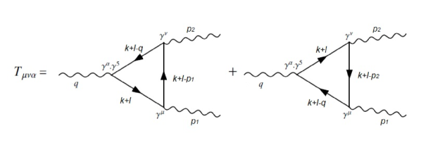
Figure 4: Triangle diagrams which contribute to the chiral anomaly. The internal lines have an arbitrary momentum route $l$.

However, this is not the only possible result for a surface term. As presented in section II, surface terms can be any number because they are differences between two divergent integrals. They are also regularization dependent. So, the scheme applied to compute the integral, symmetric integration in case of eq. (15), assigns a particular value to the surface term.

To proceed, we define

$$f(k)=Tr\left[\gamma^{\alpha}\gamma^{5}\frac{1}{\not{k}-\not{q}}\gamma^{\nu}\frac{1}{\not{k}-\not{p}_{1}}\gamma^{\mu}\frac{1}{\not{k}}\right],$$ (16)

which lead us to the result

$$\lim_{P\rightarrow\infty}f(P)=\frac{Tr[\gamma^{\alpha}\gamma^{5}\not{P}\gamma^{\nu}\not{P}\gamma^{\mu}\not{P}]}{P^{6}}=\frac{4iP_{\sigma}\epsilon^{\sigma\nu\mu\alpha}}{P^{4}}$$

and

$$T^{\alpha\mu\nu}(l,p_{1},p_{2})-T^{\alpha\mu\nu}(p_{1},p_{2})=\frac{1}{2\pi^{2}}\lim_{P\rightarrow\infty}l^{\omega}\frac{P_{\omega}P_{\sigma}}{P^{2}}\epsilon^{\sigma\nu\mu\alpha}+(\mu\leftrightarrow\nu,p_{1}\leftrightarrow p_{2})=\frac{1}{8\pi^{2}}l_{\sigma}\epsilon^{\sigma\nu\mu\alpha}+(\mu\leftrightarrow\nu,p_{1}\leftrightarrow p_{2}),$$ (17)

where we assumed an average over the surface of the sphere to use that $\frac{P_{\mu}P_{\nu}}{P^{2}}=\frac{1}{4}g^{\mu\nu}$.

We then write the general momentum routing $l$ as $l=\alpha(p_{1}+p_{2})+\beta(p_{1}-p_{2})$ and insert it in eq. (17) to find out that

$$T^{\alpha\mu\nu}(l,p_{1},p_{2})=T^{\alpha\mu\nu}(p_{1},p_{2})+\frac{\beta}{4\pi^{2}}(p_{1\sigma}-p_{2\sigma})\epsilon^{\sigma\nu\mu\alpha},$$ (18)

where we apply the Ward identity $p_{1\mu}T^{\alpha\mu\nu}(l,p_{1},p_{2})=0$ to require gauge invariance.

Alternatively, one can compute from eq. (14) for $l=0$ the identity

$$p_{1\mu}T^{\alpha\mu\nu}(p_{1},p_{2})=-\frac{1}{8\pi^{2}}p_{1\mu}p_{2\sigma}\epsilon^{\alpha\nu\mu\sigma},$$ (19)

from where we find out with the use of eq. (18) that $\beta=\frac{1}{2}$.

Finally, we can compute the chiral anomaly by contracting $q_{\alpha}$ with eq. (18):

$$q_{\alpha}T^{\alpha\mu\nu}(l,p_{1},p_{2})=q_{\alpha}T^{\alpha\mu\nu}(p_{1},p_{2})+\frac{1}{8\pi^{2}}q_{\alpha}(p_{1\sigma}-p_{2\sigma})\epsilon^{\sigma\nu\mu\alpha}$$

$$q_{\alpha}T^{\alpha\mu\nu}(l,p_{1},p_{2})=-\frac{1}{2\pi^{2}}p_{1\alpha}p_{2\sigma}\epsilon^{\sigma\nu\mu\alpha},$$ (20)

where we used the result $q_{\alpha}T^{\alpha\mu\nu}(p_{1},p_{2})=-\frac{1}{4\pi^{2}}p_{1\alpha}p_{2\sigma}\epsilon^{\sigma\nu\mu\alpha}$ that can be computed from eq. (14) for $l=0$.

Since the routing was chosen to fulfill the gauge Ward identities and get the correct result of the chiral anomaly, it looks that the momentum routing invariance is now violated because we had to choose a particular momentum in order to do this computation. In other words, if $\beta=\frac{1}{2}$ we have $l=(\alpha+1/2)p_{1}+(\alpha-1/2)p_{2}$ and it remains only one free parameter. As we are going to show in the next section, instead of choosing the momentum routing one can alternatively choose the arbitrary surface term.

V Chiral anomaly: a momentum routing invariant computation

The literature on the chiral anomaly presents its computation by several different approaches [36]-[45]. Most of them deal with the issue of $\gamma^{5}$ matrices that should be redefined in order to work with dimensional regularization, including new proposals like the rightmost position approach [39, 40] and the variant of the original Kreimer prescription with a constructively-defined $\gamma^{5}$ [38]. An overview on the various regularization schemes applied in the diagrammatic anomaly computation can be found in [33]. Besides the diagrammatic computations, there are also the Fujikawa approach based on the path integral measure transformation [41, 42] and the approach that applies differential geometry [43]. These last approaches are not diagrammatic computations and therefore they do not depend on the momentum routing of the internal lines.

In this section we derive the chiral anomaly applying the implicit regularization presented in section II. In this section, the regularization dependent content is contained in the surface term. Following the idea presented in [25], the arbitrariness inherent to some perturbative calculations in quantum field theory should be fixed based on the symmetries of the model that we want to preserve. For instance, in the neutral pion decay into two photons, we must preserve the vector Ward identities and, consequently, the axial one is violated [3, 4]. On the other hand, in the Standard Model the chiral coupling with gauge fields refers to fermion-number conservation and the axial identity must be enforced [46].

The approach presented in this section leads to a momentum routing independent result for the chiral anomaly, i. e. the computation of this anomaly is perform with arbitrary routings of the internal momenta. As the result for the scalar theory in eq. (9) and the one for QED in eq. (13), the momentum routing multiply the arbitrary surface terms. Therefore, is possible to choose a value for the surface term instead of choosing the momentum routing as in section IV.

Another issue found in triangle diagrams refer to objects like $Tr[\gamma^{\mu}\gamma^{\beta}\gamma^{\nu}\gamma^{\xi}\gamma^{\alpha}\gamma^{\lambda}\gamma^{5}]$ that appears in the amplitudes. The following identity can be used to reduce the number of Dirac $\gamma$ matrices

$$\gamma^{\mu}\gamma^{\beta}\gamma^{\nu}=g^{\mu\beta}\gamma^{\nu}+g^{\nu\beta}\gamma^{\mu}-g^{\mu\nu}\gamma^{\beta}-i\epsilon^{\mu\beta\nu\rho}\gamma_{\rho}\gamma^{5}.$$ (21)

Using eq. (21), the identities $Tr[\gamma^{\mu}\gamma^{\beta}\gamma^{\nu}\gamma^{\xi}\gamma^{5}]=4i\epsilon^{\mu\beta\nu\xi}$ and $\gamma^{5}\gamma^{\rho}\gamma^{5}=-\gamma^{\rho}$ we find the result below which is the one that most textbooks work with

$$Tr[\gamma^{\mu}\gamma^{\beta}\gamma^{\nu}\gamma^{\xi}\gamma^{\alpha}\gamma^{\lambda}\gamma^{5}]=4i(g^{\beta\mu}\epsilon^{\nu\xi\alpha\lambda}+g^{\beta\nu}\epsilon^{\mu\xi\alpha\lambda}-g^{\mu\nu}\epsilon^{\beta\xi\alpha\lambda}-g^{\lambda\alpha}\epsilon^{\mu\beta\nu\xi}+g^{\xi\lambda}\epsilon^{\mu\beta\nu\alpha}-g^{\xi\alpha}\epsilon^{\mu\beta\nu\lambda}).$$ (22)

However, it is completely arbitrary which three $\gamma$ matrices we pick up to apply equation (21). A different choice would give the result of equation (22) with Lorentz indexes permuted. Besides, the equation $\{\gamma^{5},\gamma_{\mu}\}=0$ should be avoided inside a divergent integral [29, 47] since this operation seems to fix a value for the surface term. This point of view is also shared by other works [34, 35, 44]. Therefore, we adopt a version of eq. (22) which contains all possible Lorentz structures available. This version reads

$$\frac{-i}{4}Tr[\gamma^{\mu}\gamma^{\nu}\gamma^{\alpha}\gamma^{\beta}\gamma^{\gamma}\gamma^{\delta}\gamma^{5}] =-g^{\alpha\beta}\epsilon^{\gamma\delta\mu\nu}+g^{\alpha\gamma}\epsilon^{\beta\delta\mu\nu}-g^{\alpha\delta}\epsilon^{\beta\gamma\mu\nu}-g^{\alpha\mu}\epsilon^{\beta\gamma\delta\nu}+g^{\alpha\nu}\epsilon^{\beta\gamma\delta\mu}-g^{\beta\gamma}\epsilon^{\alpha\delta\mu\nu}+$$

$$+g^{\beta\delta}\epsilon^{\alpha\gamma\mu\nu}+g^{\beta\mu}\epsilon^{\alpha\gamma\delta\nu}-g^{\beta\nu}\epsilon^{\alpha\gamma\delta\mu}-g^{\gamma\delta}\epsilon^{\alpha\beta\mu\nu}-g^{\gamma\mu}\epsilon^{\alpha\beta\delta\nu}+g^{\gamma\nu}\epsilon^{\alpha\beta\delta\mu}+$$

$$+g^{\delta\mu}\epsilon^{\alpha\beta\gamma\nu}-g^{\delta\nu}\epsilon^{\alpha\beta\gamma\mu}-g^{\mu\nu}\epsilon^{\alpha\beta\gamma\delta},$$ (23)

and it can also be obtained if we replace $\gamma^{5}$ by its definition, $\gamma^{5}=\frac{i}{4!}\epsilon^{\mu\nu\alpha\beta}\gamma_{\mu}\gamma_{\nu}\gamma_{\alpha}\gamma_{\beta}$, and take the trace.

Equation (23) has already been used in similar computations of previous works [34, 44, 45, 35]. It was also generalized to be included in $(n+1)-$point Green functions [35].

Figure 5: Triangle diagrams which contribute to the chiral anomaly. We label the internal lines with arbitrary momentum routing.

The amplitude of the Feynman diagrams of figure 5 is given by

$$T_{\mu\nu\alpha}=-i\int_{k}Tr\left[\gamma_{\mu}\frac{i}{\not{k}+\not{k}_{1}-m}\gamma_{\nu}\frac{i}{\not{k}+\not{k}_{2}-m}\gamma_{\alpha}\gamma^{5}\frac{i}{\not{k}+\not{k}_{3}-m}\right]+(\mu\leftrightarrow\nu,p\leftrightarrow q).$$ (24)

where the arbitrary routing $k_{i}$ obeys the following relations due to energy-momentum conservation at each vertex

$$k_{2}-k_{3}= p+q,$$

$$k_{1}-k_{3}= p,$$

$$k_{2}-k_{1}= q.$$ (25)

Equations (25) allow us to parametrize the routing $k_{i}$ as

$$k_{1}= \alpha p+(\beta-1)q,$$

$$k_{2}= \alpha p+\beta q,$$

$$k_{3}= (\alpha-1)p+(\beta-1)q,$$ (26)

where $\alpha$ and $\beta$ are arbitrary real numbers which map the freedom we have in choosing the momentum routing of internal lines, since any combination of $q$ and $p$ is possible as long as it is according to vertex momentum conservation in eqs. (25). Equations (25) and (26) for the other diagram are obtained by changing $p\leftrightarrow q$.

After taking the trace using equation (23), we apply the implicit regularization scheme in order to regularize the integrals coming from equation (24). The result is

$$T_{\mu\nu\alpha}=4i\upsilon_{0}(\alpha-\beta-1)\epsilon_{\mu\nu\alpha\beta}(q-p)^{\beta}+T^{finite}_{\mu\nu\alpha},$$ (27)

where $\upsilon_{0}$ is a surface term defined in section II and $T^{finite}_{\mu\nu\alpha}$ is the finite part of the amplitude whose evaluation we perform in the appendix.

We then apply the respective external momentum in equation (27) in order to obtain the Ward identities:

$$p_{\mu}T^{\mu\nu\alpha}=-4i\upsilon_{0}(\alpha-\beta-1)\epsilon^{\alpha\nu\beta\lambda}p_{\beta}q_{\lambda},$$

$$q_{\nu}T^{\mu\nu\alpha}=4i\upsilon_{0}(\alpha-\beta-1)\epsilon^{\alpha\mu\beta\lambda}p_{\beta}q_{\lambda},$$

$$(p+q)_{\alpha}T^{\mu\nu\alpha}=2mT_{5}^{\mu\nu}+8i\upsilon_{0}(\alpha-\beta-1)\epsilon^{\mu\nu\beta\lambda}p_{\beta}q_{\lambda}-\frac{1}{2\pi^{2}}\epsilon^{\mu\nu\beta\lambda}p_{\beta}q_{\lambda},$$ (28)

where $T_{5}^{\mu\nu}$ is the usual vector-vector-pseudo-scalar triangle.

The number $\upsilon_{0}(\alpha-\beta-1)$ is arbitrary since $\upsilon_{0}$ is a difference of two infinities and $\alpha$ and $\beta$ are any real numbers that we have freedom in choosing as long as equations (25) representing the energy-momentum conservation hold. We can parametrize this arbitrariness in a single parameter $a$ redefining $4i\upsilon_{0}(\alpha-\beta-1)\equiv\frac{1}{4\pi^{2}}(1+a)$. Equations (28) reads

$$p_{\mu}T^{\mu\nu\alpha}=-\frac{1}{4\pi^{2}}(1+a)\epsilon^{\alpha\nu\beta\lambda}p_{\beta}q_{\lambda},$$

$$q_{\nu}T^{\mu\nu\alpha}=\frac{1}{4\pi^{2}}(1+a)\epsilon^{\alpha\mu\beta\lambda}p_{\beta}q_{\lambda},$$

$$(p+q)_{\alpha}T^{\mu\nu\alpha}=2mT_{5}^{\mu\nu}+\frac{1}{2\pi^{2}}a\epsilon^{\mu\nu\beta\lambda}p_{\beta}q_{\lambda}.$$ (29)

From now, we will focus only in the massless theory since we would like to discuss just the quantum symmetry breaking term.

If we want to maintain gauge invariance, we choose $a=-1$ and automatically the axial identity is violated by a quantity equal to $-\frac{1}{2\pi^{2}}\epsilon^{\mu\nu\beta\lambda}p_{\beta}q_{\lambda}$, as the result obtained in the previous section. On the other hand, if we want to maintain chiral symmetry at the quantum level, we choose $a=0$ and the vectorial identities are violated. The choice $a=-1$ sets the surface term $\upsilon_{0}$ to zero. Since the surface term is zero to assure gauge invariance and it multiplies the arbitrary momentum routing, any value of the real numbers $\alpha$ and $\beta$ are possible, which makes the result momentum routing invariant. On the other hand, if gauge invariance is broken ($a=0$), there is a relation between the surface term and the momentum routing parameters $\alpha$ and $\beta$, which does not fix the momentum routing to a specific value but as in section IV the momentum routing now is not as general as possible because it only depends on the parameter $\alpha$. Furthermore, we notice that $a=-1$ is also compatible with $(\alpha-\beta-1)=0$ and $\upsilon_{0}\neq 0$. In this case, the momentum routing is related according to the eq. $\alpha=\beta+1$ and it is also possible to have gauge invariance for this specific momentum routings.

As presented in the previous section, the usual and simpler approach chooses a specific internal momentum in order to violate chiral symmetry and preserve the gauge one. Nevertheless, the implicit regularization approach and the trace symmetrization allowed us to find out that the result of the chiral anomaly is valid for any momentum routing if the arbitrary surface term $\upsilon_{0}$ is zero to assure gauge invariance. Notice, however, that is also possible to have gauge invariance for the specific momentum routing $\alpha=\beta+1$ and $\upsilon_{0}\neq 0$. Therefore, the chiral anomaly may imply in the momentum routing invariance violation but not necessarily. It is also possible to have the correct result for the chiral anomaly compatible with momentum routing invariance.

VI Scale anomaly computation for a general momentum routing $l$

The scale anomaly was computed in the past for scalar theories [48], for QED [6, 49] and also for non-abelian gauge theories [50]. Unlike the chiral anomaly, there are less debates on the scale anomaly concerning regularization schemes and different approaches. The first computations for scalar fields [48] demonstrated with perturbation theory that scale anomalies arise due to the renormalization process. The further investigation for QED used the gauge invariant vacuum polarization tensor already known at that time and showed that the trace anomaly was directly related to particle processes [6]. That original computation was confirmed with the use of loop regularization [49]. The terms that break scale symmetry at the quantum level are proportional to the beta function. So, besides being related with observables such as the hadronic $R$ ratio [6], it is also related to the renormalization group functions. We would expect therefore that the scale anomalous term does not depend on the momentum routing. Before we proceed to the computation of the diagrams, we derive below the classical breaking terms and the Ward identity of the dilatation current.

Field theories are said to be scale invariant if they are unchanged under the following scale transformations:

$$x^{\prime}=e^{\epsilon}x$$ (30)

and

$$\Phi^{\prime}(x^{\prime})=e^{-\epsilon d_{\Phi}}\Phi(x),$$ (31)

where $\epsilon$ is a scale parameter, $\Phi$ is a generic field and $d_{\Phi}$ is its scale dimension. Thus, these particular type of transformations belong to the conformal group.

We see that kinetic and interaction terms with dimensionless coupling constants are usually scale invariant and mass terms are not because masses do not transform under scale transformations. In general, it suffices to evaluate the scale dimension of the term in the Lagrangian. If its scale dimension is $4$, when the volume element $d^{4}x$ changes in the action, it compensates the change in the fields making the theory scale invariant.

The current associated with the scale invariant transformations is the dilatation current and it is equal to the trace of the energy momentum-tensor. In QED, it is possible to build a symmetric energy-momentum tensor, known as the Belinfante tensor, whose trace leads to the classical violation of the dilatation current:

$$\partial_{\mu}\mathcal{J}^{\mu}=\mathcal{T}^{\mu}_{\ \ \mu}=m\bar{\psi}\psi,$$ (32)

where $\mathcal{T}^{\mu}_{\ \ \mu}$ is the trace of the symmetric energy-momentum tensor.

Besides the mass terms, the quantum corrections also break scale symmetry because a renormalization scale is introduced in the renormalization process. For instance, in dimensional regularization, the scale parameter $\mu^{\epsilon-D}$ multiplies the divergent integrals whose dimension we changed for $D$. If one applies the scale transformations of eqs. (30) and (31), it seems that the Ward identity of the dilatation current is given by

$$-iG_{T}(0,p_{1},p_{2},...,p_{n-1})=\left(n(d_{\Phi}-4)+4-\sum_{k}^{n-1}p_{k}\frac{\partial}{\partial p_{k}}\right)G(p_{1},p_{2},...,p_{n-1}),$$ (33)

where $G_{T}(0,p_{1},p_{2},...,p_{n-1})$ and $G(p_{1},p_{2},...,p_{n-1})$ are $(n-1)$-point Green functions in the momentum space of the respective coordinate space $n-$point Green functions, $G_{T}(y,x_{1},x_{2},...,x_{n})=\langle T^{\mu}_{\mu}(y)\Phi(x_{1})\Phi(x_{2})...\Phi(x_{n})\rangle$ and $G(y,x_{1},x_{2},...,x_{n})=\langle\Phi(x_{1})\Phi(x_{2})...\Phi(x_{n})\rangle$. Note that the lower index $T$ is to emphasize that one of the fields in the expectation value is the energy-momentum tensor. However, the derivation of eq. (33) assumes $\mathcal{D}\phi=\mathcal{D}\phi^{\prime}$ in a scale transformation of the functional integral and this is not true for quantum corrections [41, 42]. As we are going to see, the identity (33) is incomplete and acquires an anomalous term.

For $n=2$ and $\Phi$ being the vector field, eq. (33) reads

$$-iG^{\mu\nu}_{T}(0,p)=\left(n(d_{\Phi}-4)+4-p^{\lambda}\frac{\partial}{\partial p^{\lambda}}\right)G^{\mu\nu}(p),$$

$$-iG^{\mu\nu}_{T}(0,p)=\left(-2-p^{\lambda}\frac{\partial}{\partial p^{\lambda}}\right)G^{\mu\nu}(p).$$ (34)

It is also possible to rewrite (34) in terms of the one-particle-irreducible (1PI) function $\Gamma^{\sigma\lambda}(p)$, related with the legged 2-point function via the equation $G_{\mu\nu}(p)=D_{\mu\sigma}(p)\Gamma^{\sigma\lambda}(p)D_{\lambda\nu}(p)$, being $D_{\mu\nu}(p)=-\frac{ig_{\mu\nu}}{p^{2}}$ the photon propagator. The Ward identity in eq. (34) can be written as

$$-i\Gamma^{\mu\nu}_{T}(0,p)=\left(2-p^{\lambda}\frac{\partial}{\partial p^{\lambda}}\right)\Gamma^{\mu\nu}(p).$$ (35)

Finally, $\Gamma^{\mu\nu}_{T}(0,p)$ corresponds to the 3-point Feynman diagram $\Delta^{\mu\nu}(0,p,-p)\equiv\Delta^{\mu\nu}(p)$ shown in figure 6, where two of the vertices are the usual ones and the other is the trace of the energy-momentum tensor $\mathcal{T}^{\mu}_{\ \ \mu}=m\bar{\psi}\psi$, $\Gamma^{\mu\nu}(p)$ corresponds to the 2-point Feynman diagram $\Pi^{\mu\nu}(p,-p)\equiv\Pi^{\mu\nu}(p)$, which is the vacuum polarization tensor. In terms of these diagrams the Ward identity can be written as:

$$\Delta^{\mu\nu}(p)=\left(2-p^{\lambda}\frac{\partial}{\partial p^{\lambda}}\right)\Pi^{\mu\nu}(p).$$ (36)

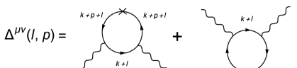
Figure 6: (a) One-loop 3-point Feynman diagram with the energy-momentum tensor as a vertex represented by a cross for a general momentum routing $l$. (b) Vacuum polarization tensor for a general momentum routing $l$.

Our purpose in this section is to compute the scale anomalous term adding a generic momentum $l$ in the internal lines of the diagrams, as presented in figure 6. So, the anomaly will be given by the violation of the equality (36) for an arbitrary $l$:

$$\Delta^{\mu\nu}(l,p)=\left(2-p^{\lambda}\frac{\partial}{\partial p^{\lambda}}\right)\Pi^{\mu\nu}(l,p).$$ (37)

The amplitudes of the Green functions involved in the relation (37) are given by

$$\Delta_{\mu\nu}(l,p)=-2\int\frac{d^{4}k}{(2\pi)^{4}}Tr[e\gamma_{\mu}S(k+l)e\gamma_{\nu}S(k+p+l)mS(k+p+l)],$$

$$i\Pi_{\mu\nu}(l,p)=\int\frac{d^{4}k}{(2\pi)^{4}}Tr[e\gamma_{\mu}S(k+l)e\gamma_{\nu}S(k+p+l)],$$ (38)

where $S(k)=\frac{i}{\not{k}-m}$ is the fermion propagator and $e$ is the electron charge.

We list all finite and regularized divergent integrals in the appendix. The result of the amplitude in eq. (38) is given by

$$\Delta_{\mu\nu}(l,p)=\Delta_{\mu\nu}(p)=\frac{m^{2}e^{2}}{2\pi^{2}}(g_{\mu\nu}Z_{0}+\iota_{0}g_{\mu\nu}p^{2}-2\iota_{1}p_{\mu}p_{\nu}-16\pi^{2}i\upsilon_{0}g_{\mu\nu}),$$ (39)

where we see that this amplitude does not depend on the general routing $l$. This is expected since the linear divergent integral of the amplitude cancels because it appears with an odd number of Dirac matrices inside the trace. So, the remaining divergent integrals are logarithmic divergent but all logarithmic divergent integrals are already momentum routing invariant.

The other amplitude we need to compute to find out the scale anomaly was already presented in section III in eq. (12). We also need to introduce the renormalization group scale $\lambda$ with the use of the scale relation below:

$$I_{log}(m^{2})=I_{log}(\lambda^{2})+b\ln\left(\frac{\lambda^{2}}{m^{2}}\right).$$ (40)

When the massless limit is taken, $\lambda$ is the only mass scale remaining. This is the part of the renormalization procedure where a renormalization scale is introduced, as the $\mu$ scale in dimensional regularization. The $\lambda$ scale is intrinsic of the implicit regularization scheme. We notice that eq. (1) splits an ultraviolet divergent integral in two infrared divergent ones in the massless limit. As a result, this scale $\lambda$ assures that no infrared divergent integral remains in the final result as we shall see below.

As an example, let us consider the sum of the logarithmic divergent integral $I_{log}(m^{2})$ with the ultraviolet finite integral $Z_{0}(p^{2},m^{2})$. A common appearance of these terms in the amplitude is $I_{log}(m^{2})-bZ_{0}(p^{2},m^{2})$ and it can be rewritten using the scale relation (40):

$$I_{log}(m^{2})-bZ_{0}(p^{2},m^{2}) =I_{log}(\lambda^{2})+b\ln\left(\frac{\lambda^{2}}{m^{2}}\right)-b\int^{1}_{0}dx\ln\left[\frac{m^{2}-p^{2}x(1-x)}{m^{2}}\right]=$$

$$=I_{log}(\lambda^{2})-b\int^{1}_{0}dx\ln\left[\frac{m^{2}-p^{2}x(1-x)}{\lambda^{2}}\right],$$ (41)

such that when we take the massless limit $m\rightarrow 0$ we find

$$\lim_{m\rightarrow 0}(I_{log}(m^{2})-bZ_{0}(p^{2},m^{2}))=I_{log}(\lambda^{2})+b\ln\left(-\frac{p^{2}}{\lambda^{2}}\right)-2b$$

and the theory is infrared safe.

With all these pieces inserted in eq.(37) and taking the massless limit, we have

$$\Delta^{\mu\nu}_{r}(l,p)-\left(2-p^{\lambda}\frac{\partial}{\partial p^{\lambda}}\right)\Pi^{\mu\nu}_{r}(l,p,\lambda)= -4e^{2}(\xi_{0}-2\upsilon_{0})\Big{(}2l^{2}g^{\mu\nu}+g^{\mu\nu}l\cdot p+l^{\nu}p^{\mu}+l^{\mu}p^{\nu}+4l^{\mu}l^{\nu}\Big{)}-8e^{2}\upsilon_{2}g^{\mu\nu}$$

$$+\frac{e^{2}}{6\pi^{2}}(p^{2}g^{\mu\nu}-p^{\mu}p^{\nu}),$$ (42)

where the index $r$ in the tensor stands for the renormalized amplitudes. It is interesting to notice that the divergent piece of eq. (37) besides being gauge invariant is scale invariant. On the other hand, the scale invariance of the finite piece is broken by a gauge invariant term.

We see in eq. (42) that in order to recover the correct result of the scale anomaly [6, 49], we must have $\upsilon_{2}=0$ and $\xi_{0}=2\upsilon_{0}$. This choice also leads to a result valid for any momentum routing $l$. This is the same condition required by gauge symmetry in section III. So, we can also conclude that gauge and momentum routing invariances imply in the correct result for the scale anomaly.

It is also interesting to notice that for massive theories the arbitrary surface term $\upsilon_{0}$ remains in eq. (39) and it is not multiplying the arbitrary momentum routing $l$ as in the examples of the previous sections or like the result of eq. (42). In this case, this surface term can not be fixed by requiring consistency of scale symmetry breaking because we have already taken the massless limit in order to compute the anomalous term.

VII Conclusions

In this work, we show that the choice of the internal momentum route in order to compute anomalies break the momentum routing invariance. However, this does not necessarily imply that momentum routing invariance of the Feynman diagrams is violated because the anomalies are physical. It is possible to compute the chiral and the scale anomalies in a momentum routing invariant way. So, even if these anomalies are present, they are still compatible with a general momentum routing. Because of the gauge and momentum routing invariance relation, we see that the latter is violated if the former is as well for some specific diagrams. This conclusion is supported by implicit regularization since the conditions that assure gauge invariance are the same that assure the momentum routing one. Nevertheless, this is not always true because in sections IV and V we show that a gauge invariant result is also compatible with a specific momentum routing choice in the case of the chiral anomaly.

As a prospect, it would be also interesting to perform the same analysis for gravitational anomalies such as the conformal anomaly in (3+1)-dimensions [51, 52] or the Einstein and Weyl anomalies in (1+1)-dimensions [53, 54]. It would be interesting to check for these gravitational theories if there is any relation between the momentum routing invariance of the Feynman diagrams and diffeomorphisms.

Appendix

We perform the computation of the finite part of the triangle diagram, $T^{finite}_{\mu\nu\alpha}$. Since it does not depend on the routing, we can choose $k_{1}=0$, $k_{2}=q$ e $k_{3}=-p$ and we have:

$$T_{\mu\nu\alpha}= -i\int_{k}Tr\left[\gamma_{\mu}\frac{i}{\not{k}-m}\gamma_{\nu}\frac{i}{\not{k}+\not{q}-m}\gamma_{\alpha}\gamma^{5}\frac{i}{\not{k}-\not{p}-m}\right]+(\mu\leftrightarrow\nu,p\leftrightarrow q)=$$

$$=-8i\upsilon_{0}\epsilon_{\mu\nu\alpha\beta}(q-p)^{\beta}+T^{finite}_{\mu\nu\alpha}$$ (43)

After taking the trace and regularizing we find out the finite part of the amplitude. We list the results of the integrals in the final part of this section. The result is

$$T^{finite}_{\mu\nu\alpha}= 4ib\{\epsilon_{\alpha\mu\nu\lambda}q^{\lambda}(p^{2}\xi_{01}(p,q)-q^{2}\xi_{10}(p,q))+\epsilon_{\alpha\mu\nu\lambda}q^{\lambda}(1+2m^{2}\xi_{00}(p,q))+$$

$$+4\epsilon_{\alpha\nu\lambda\tau}p^{\lambda}q^{\tau}[(\xi_{01}(p,q)-\xi_{02}(p,q))p_{\mu}+\xi_{11}(p,q)q_{\mu}]+(\mu\leftrightarrow\nu,p\leftrightarrow q)\},$$ (44)

where the functions $\xi_{nm}(p,q)$ are defined as

$$\xi_{nm}(p,q)=\int^{1}_{0}dz\int^{1-z}_{0}dy\frac{z^{n}y^{m}}{Q(y,z)},\\$$ (45)

with

$$Q(y,z)=[p^{2}y(1-y)+q^{2}z(1-z)+2(p\cdot q)yz-m^{2}]$$ (46)

and those functions have the property $\xi_{nm}(p,q)=\xi_{mn}(q,p)$.

The $\xi_{nm}$ functions obey the following relations which we have already used in the derivation of eq. (44)

$$q^{2}\xi_{11}(p,q)-(p\cdot q)\xi_{02}(p,q)=\frac{1}{2}\left[-\frac{1}{2}Z_{0}((p+q)^{2},m^{2})+\frac{1}{2}Z_{0}(p^{2},m^{2})+q^{2}\xi_{01}(p,q)\right],$$ (47)

$$p^{2}\xi_{11}(p,q)-(p\cdot q)\xi_{20}(p,q)=\frac{1}{2}\left[-\frac{1}{2}Z_{0}((p+q)^{2},m^{2})+\frac{1}{2}Z_{0}(q^{2},m^{2})+p^{2}\xi_{10}(p,q)\right],$$ (48)

$$q^{2}\xi_{10}(p,q)-(p\cdot q)\xi_{01}(p,q)=\frac{1}{2}[-Z_{0}((p+q)^{2},m^{2})+Z_{0}(p^{2},m^{2})+q^{2}\xi_{00}(p,q)],$$ (49)

$$p^{2}\xi_{01}(p,q)-(p\cdot q)\xi_{10}(p,q)=\frac{1}{2}[-Z_{0}((p+q)^{2},m^{2})+Z_{0}(q^{2},m^{2})+p^{2}\xi_{00}(p,q)],$$ (50)

$$q^{2}\xi_{20}(p,q)-(p\cdot q)\xi_{11}(p,q)=\frac{1}{2}\left[-\left(\frac{1}{2}+m^{2}\xi_{00}(p,q)\right)+\frac{1}{2}p^{2}\xi_{01}(p,q)+\frac{3}{2}q^{2}\xi_{10}(p,q)\right],$$ (51)

$$p^{2}\xi_{02}(p,q)-(p\cdot q)\xi_{11}(p,q)=\frac{1}{2}\left[-\left(\frac{1}{2}+m^{2}\xi_{00}(p,q)\right)+\frac{1}{2}q^{2}\xi_{10}(p,q)+\frac{3}{2}p^{2}\xi_{01}(p,q)\right],$$ (52)

where $Z_{k}(p^{2},m^{2})$ is defined as

$$Z_{k}(p^{2},m^{2})=\int^{1}_{0}dzz^{k}\ln\frac{m^{2}-p^{2}z(1-z)}{m^{2}}.$$ (53)

The derivation of the relations (47)-(52) can be simply achieved by integration by parts. There is a whole review [55] about these integrals and other integrals with integrands of larger denominators that appear in Feynman diagrams with more external legs.

Result of the integrals of sections III and VI

The result of all finite and regularized divergent integrals from sections III and VI is listed below:

$$\int_{k}\frac{k^{\mu}}{(k^{2}-m^{2})^{2}[(k-p)^{2}-m^{2}]}=-bp^{\mu}\iota_{1},$$ (54)

$$\int_{k}\frac{1}{[(k+p)^{2}-m^{2}]^{2}}=I_{log}(m^{2}),$$ (55)

$$\int_{k}\frac{1}{[(k+p)^{2}-m^{2}]}=I_{quad}(m^{2})-p^{2}\upsilon_{0},$$ (56)

$$\int_{k}\frac{1}{(k^{2}-m^{2})[(k+p)^{2}-m^{2}]^{2}}=\int_{k}\frac{1}{(k^{2}-m^{2})^{2}[(k+p)^{2}-m^{2}]}==-b\iota_{0},$$ (57)

$$\int_{k}\frac{k^{\mu}}{(k^{2}-m^{2})[(k+p)^{2}-m^{2}]^{2}}=-bp^{\mu}\iota_{1}+bp^{\mu}\iota_{0},$$ (58)

$$\int_{k}\frac{k^{\mu}k^{\nu}}{(k^{2}-m^{2})[(k+p)^{2}-m^{2}]^{2}}=\frac{1}{4}g_{\mu\nu}(I_{log}(m^{2})-\upsilon_{0})-\frac{1}{2}g_{\mu\nu}b(Z_{0}-Z_{1})-b(\iota_{0}-2\iota_{1}+\iota_{2})p^{\mu}p^{\nu},$$ (59)

$$\int_{k}\frac{k^{\mu}}{[(k+l)^{2}-m^{2}][(k+p+l)^{2}-m^{2}]}=-\left(l^{\alpha}+\frac{p^{\alpha}}{2}\right)(I_{log}(m^{2})-\upsilon_{0})+\frac{b}{2}p^{\mu}Z_{0},$$ (60)

$$\int_{k}\frac{k^{\mu}k^{\nu}}{[(k+l)^{2}-m^{2}][(k+p+l)^{2}-m^{2}]} =\frac{1}{2}g^{\mu\nu}(I_{quad}(m^{2})-\upsilon_{2})-\frac{1}{4}g^{\mu\nu}(I_{log}(m^{2})-\upsilon_{0})\left(2l^{2}+2l\cdot p+p^{2}\right)+$$

$$+\frac{1}{6}(I_{log}(m^{2})-\xi_{0})\left(g^{\mu\nu}\left(3l^{2}+3l\cdot p+p^{2}\right)+3l^{\nu}p^{\mu}+3l^{\mu}p^{\nu}+6l^{\mu}l^{\nu}+2p^{\mu}p^{\nu}\right)+$$

$$+b\left(\frac{1}{3}p^{\mu}p^{\nu}+b\frac{1}{12}p^{2}g^{\mu\nu}\right)Z_{0}-\frac{1}{4}g^{\mu\nu}p^{2}\upsilon_{0}-\frac{1}{3}b(p^{2}g^{\mu\nu}-p^{\mu}p^{\nu})\left(\frac{m^{2}}{p^{2}}Z_{0}+\frac{1}{6}\right),$$

where $Z_{n}(p^{2},m^{2})\equiv Z_{n}=\int_{0}^{1}dx\ln\frac{D(x)}{m^{2}}$, $\iota_{n}=\int^{1}_{0}dx\frac{x^{n}(1-x)}{D(x)}$, $b\equiv\frac{i}{(4\pi)^{2}}$ and $D(x)=m^{2}-p^{2}x(1-x)$.

Result of the integrals of section V

$$\int_{k}\frac{1}{(k^{2}-m^{2})[(k-p)^{2}-m^{2}][(k+q)^{2}-m^{2}]}=b\xi_{00}(p,q),$$ (63)

$$\int_{k}\frac{k^{\alpha}}{(k^{2}-m^{2})[(k-p)^{2}-m^{2}][(k+q)^{2}-m^{2}]}=b(p^{\alpha}\xi_{01}(p,q)-q^{\alpha}\xi_{10}(p,q)),$$ (64)

$$\centering\int_{k}\frac{k^{2}}{(k^{2}-m^{2})[(k-p)^{2}-m^{2}][(k+q)^{2}-m^{2}]}=\@add@centering I_{log}(m^{2})-bZ_{0}(q^{2},m^{2})+b(m^{2}-p^{2})\xi_{00}(p,q)+$$

$$+2b(p^{2}\xi_{01}(p,q)-(p\cdot q)\xi_{10}(p,q)),$$ (65)

$$\int_{k}\frac{k^{\alpha}k^{\beta}}{(k^{2}-m^{2})[(k-p)^{2}-m^{2}][(k+q)^{2}-m^{2}]}=\frac{1}{4}g^{\alpha\beta}(I_{log}(m^{2})-\upsilon_{0})-\frac{1}{4}bg^{\alpha\beta}Z_{0}(q^{2},m^{2})-$$

$$-b\Big{[}\frac{1}{2}g^{\alpha\beta}p^{2}(\xi_{00}(p,q)-3\xi_{01}(p,q)-\xi_{10}(p,q)+2\xi_{02}(p,q)+2\xi_{11}(p,q))-\xi_{02}(p,q)p^{\alpha}p^{\beta}+$$

$$+\xi_{11}(p,q)q^{\alpha}p^{\beta}+\xi_{11}(p,q)p^{\alpha}q^{\beta}-\xi_{20}(p,q)q^{\alpha}q^{\beta}+(\xi_{10}(p,q)-\xi_{11}(p,q)-\xi_{20}(p,q))g^{\alpha\beta}(p\cdot q)\Big{]},$$ (66)

$$\int_{k}\frac{k^{\alpha}k^{2}}{(k^{2}-m^{2})[(k-p)^{2}-m^{2}][(k+q)^{2}-m^{2}]}=\frac{1}{2}(p^{\alpha}-q^{\alpha})(I_{log}(m^{2})-\upsilon_{0})+\frac{1}{2}b(q^{\alpha}Z_{0}(q^{2},m^{2})-$$

$$-p^{\alpha}Z_{0}(p^{2},m^{2}))+b(m^{2}-q^{2})(p^{\alpha}\xi_{01}(p,q)-q^{\alpha}\xi_{10}(p,q))+b[q^{\alpha}p^{2}(\xi_{00}(p,q)-3\xi_{01}(p,q)-\xi_{10}(p,q)+$$

$$+2\xi_{02}(p,q)+2\xi_{11}(p,q))-2(p\cdot q)p^{\alpha}\xi_{02}(p,q)+2q^{2}p^{\alpha}\xi_{11}(p,q)+2(p\cdot q)q^{\alpha}(\xi_{10}(p,q)-$$

$$-\xi_{20}(p,q))-2q^{2}q^{\alpha}\xi_{20}(p,q))],$$ (67)

where $\int_{k}\equiv\int^{\Lambda}\frac{d^{4}k}{(2\pi)^{4}}$ and $b=\frac{i}{(4\pi)^{2}}$.

References

- [1] M. Costa, H. Panagopoulos, Phys. Rev. D 96 (2017) 034507.
- [2] G. Cynolter, E. Lendvai, Mod. Phys.Lett. A 29 (2014) 1450024.
- [3] J.S. Bell, R. Jackiw, Nuovo Cim. A 60 (1969) 47-61.
- [4] S.L. Adler, Phys. Rev. 177 (1969) 2426.
- [5] W.A. Bardeen, Phys. Rev. 184 (1969) 1848.
- [6] M.S. Chanowitz, J. Ellis, Phys. Rev. D 7 (1973) 2490.
- [7] A. Ahmad, G. Varma K., G. Sharma, J. Phys. Condens. Matter 37 (2025) 043001.
- [8] C. Corianò, M. Cretì, S. Lionetti, R. Tommasi., Phys. Rev. D 110 (2024) 025014.
- [9] H. Dang, Z. Xing, M.A. Sultan, K. Raya, L. Chang, Phys. Rev. D 108 (2023) 054031.
- [10] A. Ballon-Bayona, H. Boschi-Filho, L.A.H. Mamani, A.S. Miranda, V.T. Zanchin, Phys. Rev. D 97 (2018) 046001.
- [11] Z. Xing, H. Dang, M.A. Sultan, K. Raya, L. Chang, Phys. Rev. D 109 (2024) 054028.
- [12] H.B. Nielsen, M. Ninomiya, Phys. Lett. B 130 (1983) 389.
- [13] V.A. Zyuzin, Phys. Rev. B 95 (2017) 245128.
- [14] J. Xiong et al., Science 350 (2015) 413.
- [15] M. Hirschberger et al., Nature Materials 15 (2016) 1161.
- [16] Cheng-Long Zhang et al., Nature Communications 7 (2016) 10735.
- [17] N.P. Armitage, E.J. Mele, A. Vishwanath, Rev. of Mod. Phys. 90, 015001 (2018).
- [18] O.A. Battistel, A.L. Mota, M.C. Nemes, Mod. Phys. Lett. A 13 (1998) 1597.
- [19] G. ’t Hooft, M. Veltman, Nucl. Phys. B 44 (1972) 189.
- [20] C.G. Bollini, J.J. Giambiagi, Nuovo Cimento 12 (1972) 20.
- [21] G. Dallabona, P.G. de Oliveira, O.A. Battistel, J. Phys. G 51 (2024) 095004.
- [22] R.J.C. Rosado, A. Cherchiglia, M. Sampaio, B. Hiller, arXiv: 2404.15551 (2024).
- [23] R.J.C. Rosado, A. Cherchiglia, M. Sampaio, B. Hiller, arXiv: 2410.07944 (2024).
- [24] A.M. Burque, A.L. Cherchiglia, M. Pérez-Victoria, JHEP 08 (2018) 109.
- [25] R. Jackiw , Int. J. Mod. Phys. B 14 (2000) 2011.
- [26] B.Z. Felippe, A.P.B. Scarpelli, A. R. Vieira, J.C.C. Felipe, Eur. Phys. J. C 82 (2022) 583.
- [27] A.L. Cherchiglia, M. Sampaio, M.C. Nemes, Int. J. Mod. Phys. A 26 (2011) 2591-2635.
- [28] M.E. Peskin, D. Schroeder, An Introduction to Quantum Field Theory, Addison-Wesley, 1995.
- [29] A.C.D. Viglioni, A.L. Cherchiglia, A.R. Vieira, B. Hiller, M. Sampaio, Phys. Rev. D 94 (2016) 065023.
- [30] L.C. Ferreira, A.L. Cherchiglia, B. Hiller, M. Sampaio, M.C. Nemes, Phys. Rev.D 86 (2012) 025016.
- [31] A.R. Vieira, A.L. Cherchiglia, M. Sampaio, Phys. Rev. D 93 (2016) 025029.
- [32] A. Zee, Quantum Field Theory in a Nutshell, Cambridge University Press, 2003.
- [33] R.A. Bertlmann, Anomalies in Quantum Field Theory, Oxford University Press, 1996.
- [34] G. Cynolter and E. Lendvai, Mod. Phys. Lett. A 26 (2011) 1537.
- [35] J.F. Thuorst, L. Ebani, T.J. Girardi, Annals of Phys. 468 (2024) 169725.
- [36] V. Elias, G. McKeon, R. B. Mann, Nucl. Phys. B 229 (1983) 487.
- [37] H.-L. Yu, W. B. Yeung, Phys. Rev. D 35 (1987) 3955.
- [38] L. Chen, JHEP 2023 (2023) 11, 30.
- [39] Er-Cheng Tsai, Phys. Rev. D 83 (2011) 025020.
- [40] Er-Cheng Tsai, Phys. Rev. D 83 (2011) 065011.
- [41] K. Fujikawa, Phys. Rev. Lett. 42 (1979) 1195.
- [42] K. Fujikawa, Phys. Rev. D 21 (1980) 2848.
- [43] B. Zumino, W. Yong-Shi, A. Zee, Nucl. Phys. B 239 (1984) 477.
- [44] F. del Aguila, M. Perez-Victoria, Acta Phys. Pol. B 29 (1998) 2857.
- [45] Y. L. Ma, Y. L. Wu, Int. J. Mod. Phys. A 21 (2006) 6383.
- [46] G. t’Hooft, Phys. Rev. Lett. 37 (1976) 8.
- [47] A.L. Cherchiglia, Nucl. Phys. B 987 (2023) 116104.
- [48] C.G. Callan, Phys. Rev. D 2 (1970) 1541.
- [49] J.-W. Cui, Y.-L. Ma, Y.-L. Wu, Phys. Rev. D 84 (2011) 025020.
- [50] J.C. Collins, A. Duncan, S.D. Joglekar, Phys. Rev. D 16 (1977) 438.
- [51] A.R. Vieira, J.C.C. Felipe, G. Gazzola, M. Sampaio, Eur. Phys. J. C 75 (2015) 7, 338.
- [52] M. Asorey, E.V. Gorbar, I.L. Shapiro, Class. Quant. Grav. 21 (2003) 163-178.
- [53] R. A. Bertlmann, E. Kohlprath, Phys. Lett. B 480 (2000) 200-206.
- [54] L.A.M. Souza, M. Sampaio, M.C. Nemes, Phys. Lett. B 632 (2006) 717-724.
- [55] O.A. Battistel, G. Dallabona, Eur. Phys. J. C 45 (2006) 721.