A sensitivity analysis approach to principal stratification with a continuous longitudinal intermediate outcome: Applications to a cohort stepped wedge trial

Abstract

Causal inference in the presence of intermediate variables is a challenging problem in many applications. Principal stratification (PS) provides a framework to estimate principal causal effects (PCE) in such settings. However, existing PS methods primarily focus on settings with binary intermediate variables. We propose a novel approach to estimate PCE with continuous intermediate variables in the context of stepped wedge cluster randomized trials (SW-CRTs). Our method leverages the time-varying treatment assignment in SW-CRTs to calibrate sensitivity parameters and identify the PCE under realistic assumptions. We demonstrate the application of our approach using data from a cohort SW-CRT evaluating the effect of a crowdsourcing intervention on HIV testing uptake among men who have sex with men in China, with social norms as a continuous intermediate variable. The proposed methodology expands the scope of PS to accommodate continuous variables and provides a practical tool for causal inference in SW-CRTs.

Keywords: Causal inference; cluster randomized trial; HIV testing and prevention; principal causal effect; stepped wedge design; sensitivity analysis

1 Introduction and Literature Review

In many scientific applications, it is of interest to investigate the causal pathway underlying the total treatment effect when an intermediate variable is present. Several different types of intermediate variables have been studied in the prior literature, including but not limited to treatment compliance (Angrist et al. (1996), Roy et al. (2008), Jin and Rubin (2008)), death as a terminal event (Dai et al. (2012); Xu et al. (2022); Nevo and Gorfine (2022)) and secondary outcomes (Kim et al. (2019)).

There exist several frameworks that can address intermediate variables. Among them, a useful framework is causal mediation analysis that explores the causal relationship under an intervention on the intermediate variable, in terms of direct and indirect effects (VanderWeele (2008); Imai et al. (2010)). An alternative approach, principal stratification (Frangakis and Rubin (2002)), focuses on the causal effect within strata defined by potential values of the intermediate variable. Principal stratification uses the potential outcomes of the intermediate variable under different arms of treatment to define subgroups, and the principal causal effects (PCEs) are the comparison of the outcome within subgroups.

Under the latter framework, much of the prior literature focused on point and interval identification of the PCEs with a binary intermediate variable. A popular method for identification is based on an instrumental variable (Angrist et al. (1996)), typically under the monotonicity and the exclusion restriction assumptions. Roy et al. (2008) introduced a weaker version of the monotonicity assumption. Ding and Lu (2017) relaxed the exclusion restriction assumption by introducing the general principal ignorability assumption given baseline covariates, which is untestable based on the observed data alone. Under general principal ignorability, one can calculate the principal scores—analogues of the propensity scores—as functions of baseline covariates to point identify the PCEs. To relax the untestable structural assumptions, others have also used a parametric mixture approach to empirically identify the PCEs (e.g., Imbens and Rubin (1997); Zhang et al. (2009); Frumento et al. (2012)).

Continuous intermediate variables introduce additional challenges for principal stratification analysis, compared to binary or categorical variables. Most of the existing methods either dichotomized the intermediate variable (Baccini et al. (2017)), or assumed a fully parametric model for the joint distribution of the potential intermediate variables (Magnusson et al. (2019)). However, as discussed in Schwartz et al. (2011), the former is subject to information loss and arbitrary choice of the cutoff point and the latter is often inadequate to represent complex distributional and clustering features. In contrast, Schwartz et al. (2011) treated principal stratification as an incomplete data problem, and use a Dirichlet process mixture to address latent clustering features. Kim et al. (2019) studied multiple continuous intermediate variables and propose a Gaussian copula assumption and an additional homogeneity assumption to identify the PCE. Antonelli et al. (2023) extended the PS framework to studies with continuous treatments and continuous intermediate variables.

While there has been extensive development of principal stratification methods with cross-sectional data, relatively fewer efforts have focused on principal stratification with longitudinal data, with the following few exceptions. Yau and Little (2001) studied the causal effects in the presence of treatment noncompliance in a longitudinal setting. Their framework focused on a time-fixed treatment and assumed away defiers and always-takers. Frangakis et al. (2004) considered studies with time-varying treatment and compliance. However, their approach did not account for possible correlations among repeated measurements taken on the same unit. Their identification result depends on two strong assumptions, multilevel monotonicity and a compound exclusion restriction, which are generalization of standard monotonicity and exclusion restriction assumptions to accommodate a time-varying treatment. Lin et al. (2008, 2009) proposed a hierarchical latent class structure that consists of time-varying compliance nested in classes of longitudinal compliance trends that are time-invariant in a parametric setting. Dai et al. (2012) considered a partially Hidden Markov model on compliance behavior with a time-to-event endpoint. Despite their focus on the longitudinal data structure, these prior efforts have been restricted to a binary intermediate variable—typically noncompliance, and have not been expanded to address a continuous intermediate variable.

2 Motivating Data Example and Objective

Our study is motivated by a closed-cohort stepped wedge cluster randomized trial (SW-CRT) in the presence of a continuous intermediate variable. SW-CRTs are a recent variant of cluster randomized designs that are increasingly common for evaluating healthcare interventions (Nevins et al. (2024)). In a SW-CRT, clusters are randomized to different time points corresponding to when the intervention starts. All clusters start with no treatment and eventually receive the treatment. These features allow each cluster to serve as its own control and can facilitate cluster recruitment and stakeholder engagement especially when the intervention is perceived to be beneficial (Hemming and Taljaard (2020)). Specifically, Tang et al. (2018) reported a completed SW-CRT which evaluated the impact of a newly-developed crowdsourcing HIV intervention on HIV testing uptake among men who have sex with men in eight Chinese cities, from August 2016 to August 2017. The crowdsourcing intervention included a multimedia HIV testing campaign, an online HIV testing service, and local testing promotion campaigns tailored for men who have sex with men. The study design is a closed-cohort SW-CRTs, which recruited a closed-cohort of men who have sex with men prior to randomization of cities. The intervention was initiated for pairs of cities at 3-month intervals, and each pair of cities received the intervention for 3 consecutive months. In total, the study collected data at baseline followed by four time points over 12 months, and enrolled a total of 1,381 participants as a closed cohort.

The primary outcome of this study was the proportion of participants who tested for HIV over the previous 3 months. Figure 1(a) shows the HIV testing proportion in different time periods. An important secondary outcome was the sensitivity to HIV testing social norms, which was measured by six items asking participants about their perceived social norm regarding HIV testing. The HIV testing social norms have been studied as an intermediate outcome (or mediator) and proved to have a significant relationship with the uptake of HIV testing (Babalola (2007); Perkins et al. (2018); Zhao et al. (2018)). Figure 1(b) shows that HIV testing social norms score in different time periods. In the context of the SW-CRT reported by Tang et al. (2018), our goal is to investigate whether the causal effects of crowdsourcing intervention on the HIV testing uptake differ across different strata defined by social norm, under a principal stratification framework, to assess the role of social norm.

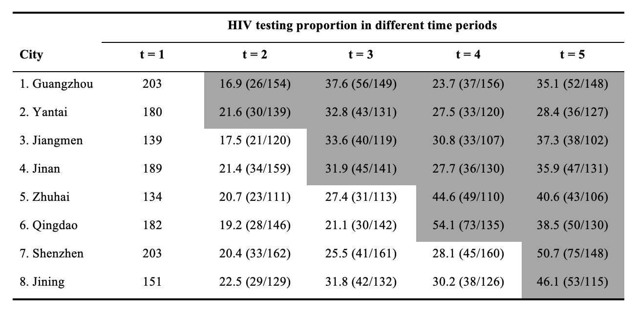
(a) HIV testing proportion (%); In the baseline period ($t=1$), the HIV testing proportion is zero.

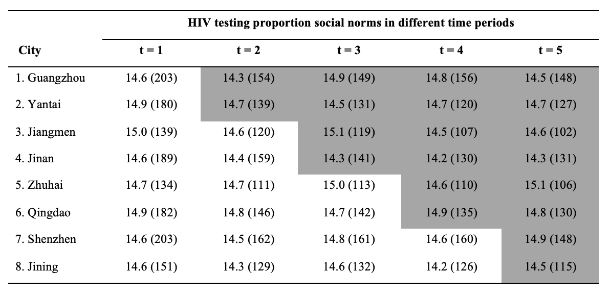
(b) HIV testing social norms summarized by cluster-period means

Figure 1: Summary statistics on HIV testing proportion (%) and social norms by city and time periods. Shaded cells represent intervention cluster-periods and white cells represent control cluster-periods.

To provide insights into the role of social norm in the crowdsourcing HIV intervention study, we pursue the potential outcomes framework, and propose specific principal causal effect estimands of interest to address a continuous intermediate outcome in the context of closed-cohort SW-CRTs. We then propose new structural assumptions to achieve point identification of the principal causal effect estimands under a sensitivity framework. These include a copula assumption that addresses the joint distribution of the potential intermediate variables under treatment and control conditions, and a marginal structural assumption that addresses the relationship between potential outcome and potential intermediate variables. To implement our procedure, we exploit a unique feature of SW-CRTs that the intermediate variable and outcome are observable in both treatment arms at different time points, which provides useful information to calibrate values for sensitivity parameters in the structural assumptions. We then consider random-effects models that are commonly used to estimate treatment effects in SW-CRTs (Li et al., 2021) and pursue a Bayesian framework for inference. The Bayesian inferential framework is also attractive as it can accomodate monotone missing data (under an ignorability assumption), which is present in the crowdsourcing HIV intervention study. Different from the existing literature discussed in Section 1, our development represents the first effort to simultaneously addresses the longitudinal data structure (arising from the closed-cohort stepped wedge design) and a continuous intermediate outcome.

The remainder of this paper is organized as follows. Section 3 introduces our proposed methodology, including notation specific for closed-cohort SW-CRTs, proposed causal estimands, structural assumptions, and new identification result. Section 4 discusses the observed data modeling approach and ways to calibrate sensitivity parameters using observed data. In Section 5, we apply our proposed methodology to analyze the crowdsourcing HIV intervention study to provide additional insights into the role of social norm in explaining the causal effects on HIV testing uptake. Finally, Section 6 provides a discussion of the implications of our findings and potential areas for future research.

3 A sensitivity analysis framework for principal stratification with a longitudinal continuous intermediate variable

3.1 Notation for SW-CRTs

We consider a closed-cohort SW-CRT where all participating individuals are identified prior to cluster randomization. We first discuss our proposed methods in the absence of attrition; extensions to address monotone missing data will be discussed in Section 4.3 in the context of the crowdsourcing HIV intervention study. We use $i$ to denote each individual, $j$ to denote cluster and $t$ to denote the discrete time period. As we consider a closed-cohort design, individuals ($i$) are nested in clusters ($j$), which are cross-classified by periods ($t$). Let $Z_{jt}$ be the indicator of intervention status of cluster $j$ at time $t$. Due to the staggered rollout design feature, $Z_{jt}\geq Z_{j,t-1}$ for any $j$ and $t$. Furthermore, we let $M_{ijt}$ and $Y_{ijt}$ denote the intermediate variable and the outcome for individual $i$ in cluster $j$ measured during period $t$, and we assume that the cluster-level intervention $Z_{jt}$ happens prior to $M_{ijt}$, which also temporally proceeds $Y_{ijt}$ and hence is an intermediate outcome. Moreover, define $\overline{M}_{ijt}=(M_{ij1},M_{ij2},\dots,M_{ijt})$ as the history of intermediate variables, $\overline{M}_{ij}=\overline{M}_{ijT}$, and similarly, $\overline{Y}_{ijt}=(Y_{ij1},Y_{ij2},\dots,Y_{ijt})$, $\overline{Z}_{jt}=(Z_{j1},Z_{j2},\dots,Z_{jt})$, $\overline{Y}_{ij}=\overline{Y}_{ijT}$, and $\overline{Z}_{j}=\overline{Z}_{jT}$. See Figure 1 for a schematic illustration of the stepped wedge design.

3.2 Standard Assumptions for SW-CRTs

We use a potential outcomes framework (Rubin (1974)) to clarify several standard assumptions for SW-CRTs. Let $\overline{\bm{Z}}=(\overline{Z}_{1},\overline{Z}_{2},\dots,\overline{Z}_{J})$ be $T\times J$ matrix of treatment assignments, where $\overline{Z}_{j}\in\mathcal{Z}$ denote the treatment sequence of cluster $j$, with $\mathcal{Z}$ being its support. And let $\overline{M}_{ij}(\overline{\bm{Z}})$ be the vector of potential outcomes of the intermediate variable of individual $i$ in cluster $j$ given treatment $\overline{\bm{Z}}$, and similarly for $\overline{Y}_{ij}(\overline{\bm{Z}})$. We first make the assumption that the potential outcomes and potential intermediate variables of cluster $j$ are independent of treatment sequences of other clusters (Rubin (1980)); in other words, there is no interference among clusters.

Assumption 1 (SUTVA).

For any two matrices of treatment $\overline{\bm{z}}$, $\overline{\bm{z}}^{\prime}$, if $\overline{z}_{j}=\overline{z}^{\prime}_{j}$, then $\overline{M}_{ij}(\overline{\bm{z}})=\overline{M}_{ij}(\overline{\bm{z}}^{\prime})$, $\overline{Y}_{ij}(\overline{\bm{z}})=\overline{Y}_{ij}(\overline{\bm{z}}^{\prime})$.

Using the stable unit treatment value assumption (SUTVA) we can simplify notation and write the potential outcomes of interest as $\overline{Y}_{ij}(\overline{z}_{j}),\overline{M}_{ij}(\overline{z}_{j})$. This assumption is also referred to as cluster-level SUTVA (Chen and Li (2024)). Additionally, the treatment sequence is randomly assigned to clusters, which is formalized by the following assumption.

Assumption 2 (Stepped wedge randomization).

For any possible treatment sequence $\overline{z}_{j}$, $\overline{\bm{Z}}\perp(\overline{Y}_{ij}(\overline{z}_{j}),\overline{M}_{ij}(\overline{z}_{j}))$.

This assumption states that the assignment of treatment sequences does not depend on any potential intermediate variables or final outcomes, and is completely random. Finally, we make the following assumption to rule out anticipation effects.

Assumption 3 (No anticipation).

For any treatment arms $\overline{z}_{j},\overline{z}_{j}^{\prime}$, if $\overline{z}_{jt}=\overline{z}_{jt}^{\prime}$, then $\overline{Y}_{ijt}(\overline{z}_{j})=\overline{Y}_{ijt}(\overline{z}_{j}^{\prime})$, $\overline{M}_{ijt}(\overline{z}_{j})=\overline{M}_{ijt}(\overline{z}_{j}^{\prime})$.

The no-anticipation assumption posits that potential outcomes and potential intermediate variables do not depend on future treatment assignments. Thus, the potential outcome and potential intermediate variable at any given time can at most depend only on the treatment assignments up to and including that time point. Under this assumption, we can further simplify the notation for potential outcomes to $\overline{Y}_{ijt}(\overline{z}_{jt})$ and $\overline{M}_{ijt}(\overline{z}_{jt})$. This assumption has been considered by Athey and Imbens (2022) within the context of the randomized difference-in-differences framework. The no-anticipation assumption is also standard in previous literature for stepped wedge designs in the absence of an intermediate variable (Chen and Li, 2024; Wang et al., 2024).

3.3 Principal stratification

Principal stratification compares (e.g., the difference in mean of) the potential outcomes for subgroups defined by the potential values of the intermediate variable (Frangakis and Rubin (2002)). In a SW-CRT, the cluster-level treatment is a time-varying exogenous variable. Table 1 presents the possible treatment assignments for an example trial with $T=5$.

Table 1: Possible treatment sequences at each time period in an example SW-CRT with a total of $T=5$ periods. Note that time $1$ is the baseline period, where no clusters are exposed under the intervention; at time $5$, all clusters are exposed under the intervention. The intervention sequences in bold are the principal strata of interest in our causal estimand.

Time	Control	Intervention
1	$0$	-
2	$(0,0)$	$(0,1)$
3	$(0,0,0)$	$\bm{(0,0,1)},(0,1,1)$
4	$(0,0,0,0)$	$\bm{(0,0,0,1)},(0,0,1,1),(0,1,1,1)$
5	-	$\bm{(0,0,0,0,1)},(0,0,0,1,1),(0,0,1,1,1),(0,1,1,1,1)$

Under no anticipation, the potential values of $Y$ and $M$ are defined by treatment sequence up to time $t$ (Assumption 3). We consider the contrast between the potential outcomes of $Y$ for the following treatment sequence $(\underbrace{0,0,\dots,0}_{t-1},z)$, which corresponds to comparing the counterfactual scenario when all clusters starting the treatment at time $t$, versus that when all clusters starting the treatment later than time $t$, as shown in bold formatting in Table 1. Under this setup, we are interested in examining the short-term causal effect of the one-time treatment initiation, rather than the long-term causal effect due to prolonged exposure to the treatment. By focusing on the contrast between clusters that start the treatment at time $t$ and those that have not yet started, we can isolate the immediate impact of the intervention and assess its effectiveness at the time of initial implementation. We refer this as the treatment initiation causal effect at a specific period $t$. Importantly, even though we define the treatment initiation causal effect as the estimand of primary interest, we are not assuming the causal effect is constant over exposure time, as in standard regression analysis of SW-CRTs (Hussey and Hughes, 2007). Rather, as we elaborate in Section 4, the models we considered will allow for time-varying treatment effects along the lines of Kenny et al. (2022), Maleyeff et al. (2023), and Wang et al. (2024). However, an extension of estimands especially under the principal stratification framework to address long-term causal effect is beyond the scope of this development and will be pursued in future work.

Focusing on the short-term effect, we let $\underline{z}_{t}=(\underbrace{0,0,\dots,0}_{t-1},z)$. To address the role of the intermediate variable, we consider principal strata of defined as $S_{ijt}=(M_{ijt}(\underline{0}_{t}),M_{ijt}(\underline{1}_{t}))$. In our crowdsourcing HIV intervention study, the causal estimand of interest is the change in HIV self-testing rate from control to intervention among strata defined by the social norm. To precisely define our estimands, we include the following additional assumption.

Assumption 4 (Super-population sampling).

Denote $N_{j}$ as the size of the closed cohort in each cluster, and $\overline{W}_{j}=\{\overline{Y}_{ij}(\overline{z}_{j}),\overline{M}_{ij}(\overline{z}_{j}),N_{j};i=1,\ldots,N_{j},\overline{z}_{j}\in\mathcal{Z}\}$ as the complete data vector for each cluster. Then $\{W_{1},\ldots,W_{J}\}$ are independent and identically distributed draws from a population distribution with finite second moments. Within each cluster, the individual potential outcome and intermediate variable concerning the short-term effects $\{\overline{Y}_{ijt}(\underline{z}_{t}),\overline{M}_{ijt}(\underline{z}_{t}):z\in\{0,1\}\}$ for $i=1,\ldots,N_{j}$ and $j=1,\ldots,T$ are identically distributed given cohort size $N_{i}$.

Under Assumption 4, the marginal and conditional expectations of individual potential outcomes are well-defined, and we can write the period-specific associative and dissociative effects (VanderWeele (2008)), as below

Dissociative effect: $$E(Y_{ijt}(\underline{1}_{t})-Y_{ijt}(\underline{0}_{t})|M_{ijt}(\underline{1}_{t})=M_{ijt}(\underline{0}_{t}))$$

Associative effect: $$E(Y_{ijt}(\underline{1}_{t})-Y_{ijt}(\underline{0}_{t})|M_{ijt}(\underline{1}_{t})\neq M_{ijt}(\underline{0}_{t})).$$

In Supplementary Section A, we show that these principal causal effect estimands align with the concept of cluster-average treatment effect estimands defined in Kahan et al. (2024) and Wang et al. (2024). These estimands measure the degree to which the intervention causally influences outcomes depending on whether the intervention has a causal impact on the intermediate variable. A non-zero associative effect suggests a causal mechanism where the intervention alters the outcome via modifications in the intermediate variable, similar to the indirect effect in causal mediation analysis, whereas a non-zero dissociative effect indicates a direct effect on the outcome that works without changing the intermediate variable.

When the intermediate variable is continuous, the probability of the event $M_{ijt}(\underline{1}_{t})=M_{ijt}(\underline{0}_{t})$ is 0. To accommodate continuous intermediate values, we consider the following slightly modified principal causal effect estimand (Zigler et al. (2012); Kim et al. (2019)):

$$\text{$t$th PCE among subpopulation $\mathcal{I}$: }E(Y_{ijt}(\underline{1}_{t})-Y_{ijt}(\underline{0}_{t})|M_{ijt}(\underline{1}_{t})-M_{ijt}(\underline{0}_{t})\in\mathcal{I}),$$ (1)

where $\mathcal{I}$ denote the subpopulation of interest defined by the difference in $M_{ijt}(\underline{0})$ and $M_{ijt}(\underline{1})$. Note that the dissociative effect can now be defined on the principal strata where potential changes in the intermediate variables are less than some threshold instead of principal stratum with strict equality to accommodate continuous intermediate values, e.g., $\mathcal{I}=(-\delta,\delta)$ for some $\delta>0$.

3.4 Identification under a sensitivity analysis framework

To point identify (1), we consider two additional structural assumptions that include interpretable sensitivity parameters in the context of SW-CRTs. By construction of the principal causal estimands, we first need to identify the joint distribution of potential intermediate variables. Because the observed data do not provide any information on the joint, only their margins, we consider an assumption to describe the joint (Efron and Feldman (1991); Jin and Rubin (2008)). Here, we adopt a copula approach, formalized through the following assumption (Bartolucci and Grilli (2011); Daniels et al. (2012)).

Assumption 5 (Copula for intermediate variables).

For all $t$, given sensitivity parameter $\rho$ describing the correlations between $M_{ijt}(\underline{1}_{t})$ and $M_{ijt}(\underline{0}_{t})$ and an assumed copula $C_{\rho}$,

$$P(M_{ijt}(\underline{0}_{t}),M_{ijt}(\underline{1}_{t})) =C_{\rho}\left\{P(M_{ijt}(\underline{0}_{t})),P(M_{ijt}(\underline{1}_{t}))\right\}$$ (2)

The copula allows us to identify the joint of $M_{ijt}(\underline{0}_{t})$ and $M_{ijt}(\underline{1}_{t})$ without any restriction on their marginals. In Section 4.2, we will provide guidance on calibrating the sensitivity parameter $\rho$ based on the observed data in a SW-CRT. In practice, we recommend a Gaussian copula for a continuous intermediate variable. In this case, $\rho$ can be regarded as the intra-cluster correlation for the same individual across different treatment conditions in a cross-world scenario. To identify PCE, it is also necessary to identify the distribution of the outcome value in the principal strata. Inspired by Heagerty (1999), we construct the following identifying assumption.

Assumption 6 (Marginal structural assumption).

For all $t$, given sensitivity parameter $\lambda_{z}$,

$$g(E(Y_{ijt}(\underline{z}_{t})|M_{ijt}(\underline{(1-z)}_{t})=m^{*},M_{ijt}(\underline{z}_{t})=m))=\Delta_{ijt}(m,z)+\lambda_{z}m^{*}.$$ (3)

Model (3) describes the structural relationship between potential outcomes within strata defined by the potential intermediate variables, and is marginal with respect to cluster-periods (hence not conditioning on any latent random effects). The parameter $\Delta_{ijt}$ is specified indirectly through the marginal means $E(Y_{ijt}(\underline{z}_{t})|M_{ijt}(\underline{z}_{t})=m)$, and can be recovered numerically as a function of $m$ and $z$. The sensitivity parameter $\lambda_{z}$ represents a shift in the conditional mean on the link function scale as a function of $m^{*}$ for a given $z$. In Section 4.2, we will introduce a method to calibrate $\lambda_{z}$ that leverages the unique data structure of SW-CRTs. Under the aforementioned assumptions, we can point identify our target PCE estimand among subpopulation $\mathcal{I}$ by the following theorem.

Theorem 1 (Identification).

Under Assumptions 1 - 6, the estimand in (1) is point identified:

$$\quad E(Y_{ijt}(\underline{1}_{t})-Y_{ijt}(\underline{0}_{t})|M_{ijt}(\underline{1}_{t})-M_{ijt}(\underline{0}_{t})\in\mathcal{I})$$

$$=\frac{\int_{\mathcal{I}}[g^{-1}(\Delta_{ijt}(m_{1},1)+\lambda_{1}m_{0})-g^{-1}(\Delta_{ijt}(m_{0},0)+\lambda_{0}m_{1})]dP(M_{ijt}(\underline{1}_{t}),M_{ijt}(\underline{0}_{t}))}{\int_{\mathcal{I}}dP(M_{ijt}(\underline{1}_{t}),M_{ijt}(\underline{0}_{t})))}.$$

Supplementary Section B provides a sketch of the proof for this theorem. The essential ingredients of the identification formula include the marginal structural model (3) and the joint distribution of the intermediate variables through the copula structure (2), with the set of interpretable sensitivity parameters $\{\lambda_{1},\lambda_{0},\rho\}$.

4 Model specification, Sensitivity parameters, and Inference

4.1 Observed data model and identification

To implement the approach for estimating the PCE, we first introduce an observed data model that incorporates both the outcome and the intermediate variable. This model builds upon the mixed-effects model, which is widely used for analyzing SW-CRTs in the absence of intermediate outcomes (Li et al. (2021)). Although our structural assumptions can accommodate treatment effect that varies over duration of the exposure (Kenny et al., 2022; Maleyeff et al., 2023; Wang et al., 2024), the crowdsourcing HIV intervention is a short exposure and hence is unlikely to lead to a delayed or cumulative treatment effect over duration. Therefore, to avoid over-fitting, we consider a simpler treatment effect structure in our model below. Our approach specifies fixed effects for the secular trend and the intervention effect, along with random effects to account for the correlation among observations collected from the same cluster and across time. Specifically, we include random intercepts at the cluster level to capture between-cluster variability and at the individual level to account for the correlation among repeated measurements from the same individual within a cluster. Since we have a continuous mediator and a binary outcome in the crowdsourcing HIV intervention study, we consider the following observed data models,

$$M_{ijt} =\eta_{1t}+\gamma_{1}Z_{jt}+\alpha_{1j}+\phi_{1ij}+\epsilon_{ijt},$$ (4)

$$\operatorname{logit}\left(\mu_{Y,ijt}\right) =\eta_{2t}+\beta_{1}Z_{jt}+\beta_{2}M_{ij,t-1}+\beta_{3}Z_{jt}M_{ij,t-1}+\beta_{4}Z_{j,t-1}M_{ij,t-1}+\alpha_{2j}+\phi_{2ij},$$ (5)

where $(\alpha_{1j},\alpha_{2j})\sim N(\bm{0},\Sigma_{\alpha})$ is the random cluster effect, $(\phi_{1ij},\phi_{2ij})\sim N(\bm{0},\Sigma_{\phi})$ is the random effect for the longitudinal measures from individual $i$, and $\epsilon_{ijt}\sim N(0,\sigma^{2}_{\epsilon})$ is the residual error. The parameters, $\eta_{1t},\eta_{2t}$ represent the fixed effects of time.

Suppose the PCE is defined among the subpopulation $\mathcal{I}=[a,b]$ for some pre-specified constants $a$, $b$, then by (4), $M_{ijt}(\underline{z}_{t})$ follows a normal distribution, and $E(M_{ijt}(\underline{z}_{t}))=\eta_{1t}+\gamma_{0}+\gamma_{1}z$, $\text{Var}(M_{ijt}(\underline{z}_{t}))=\Sigma_{\alpha,11}+\Sigma_{\phi,11}+\sigma_{\epsilon}^{2}$, where $\Sigma_{\alpha,lk}$ and $\Sigma_{\phi,lk}$ are the $(i,k)$th element of the covariance matrices $\Sigma_{\alpha}$ and $\Sigma_{\phi}$, respectively. Therefore, under a given value of the sensitivity parameter $\rho$, Assumption 5 allows us to express the denominator in the identification formula given by Theorem 1 as

$$\int_{\mathcal{I}} dP(M_{ijt}(\underline{1}_{t}),M_{ijt}(\underline{0}_{t}))=P(a\leq M_{ijt}(\underline{1}_{t})-M_{ijt}(\underline{0}_{t})<b)$$

$$= \Phi\left(\frac{b-\gamma_{1}}{\sqrt{2(1-\rho)(\Sigma_{\alpha 11}+\Sigma_{\phi 11}+\sigma_{\epsilon}^{2})}}\right)-\Phi\left(\frac{a-\gamma_{1}}{\sqrt{2(1-\rho)(\Sigma_{\alpha 11}+\Sigma_{\phi 11}+\sigma_{\epsilon}^{2})}}\right).$$

To explicitly express the numerator in the identification formula given by Theorem 1, we first obtain an expression for $E(Y_{ijt}(\underline{z}_{t})|M_{ijt}(\underline{z}_{t})=m)$ under the observed data model specifications. Since $(\alpha_{2j}+\phi_{1j})|M_{ijt}=m,\underline{Z}_{jt}=\underline{z}_{t}$ follows a normal distribution, with mean and variance

$$E(\alpha_{2j}+\phi_{2ij}|M_{ijt}=m,\underline{Z}_{jt}=\underline{z}_{t}) =\frac{\Sigma_{\alpha,12}+\Sigma_{\phi,12}}{\sigma^{2}_{\epsilon}+\Sigma_{\alpha,11}+\Sigma_{\phi,11}}(m-\eta_{1t}-\gamma_{0}-\gamma_{1}z),$$

$$\text{Var}(\alpha_{2j}+\phi_{2ij}|M_{ijt}=m,\underline{Z}_{jt}=\underline{z}_{t}) =\Sigma_{\alpha,22}+\Sigma_{\phi,22}-\frac{(\Sigma_{\alpha,12}+\Sigma_{\phi,12})^{2}}{\sigma^{2}_{\epsilon}+\Sigma_{\alpha,11}+\Sigma_{\phi,11}},$$

then we have $E(Y_{ijt}|M_{ijt}=m,\underline{Z}_{jt}=\underline{z}_{t})=E(\operatorname{expit}(\eta_{2t}+\beta_{0}+\beta_{1}z+\beta_{2}m+\beta_{3}mz+\alpha_{2j}+\phi_{2ij})|M_{ijt}=m)$. We approximate this last expression via $\sum_{k=1}^{20}w_{k}\operatorname{expit}(\eta_{2t}+\beta_{0}+\beta_{1}z+\beta_{2}m+\beta_{3}mz+s_{k})$, where $w_{k}$ and $s_{k}$ are from implementing Gaussian-Hermite quadrature based on the conditional normal distribution of $(\alpha_{2j}+\phi_{1j})|M_{ijt},\underline{Z}_{jt}$.

Finally, in Supplementary Section B, we establish the following convolution equation in proving Theorem 1,

$$E(Y_{ijt}|M_{ijt}=m,\overline{Z}_{jt}=\underline{z}_{t})$$ (6)

$$= \int g^{-1}(\Delta_{ijt}(m,z)+\lambda_{z}M_{ijt}(\underline{(1-z)}_{t}))dP(M_{ijt}(\underline{(1-z)}_{t})|M_{ijt}(\underline{z}_{t})=m).$$ (7)

By model (4) and (5), the above convolution equation gives:

$$0 =-E(Y_{ijt}|M_{ijt}=m,\overline{Z}_{jt}=\underline{z}_{t})+\int\frac{e^{\Delta_{ijt}(m,z)+\lambda_{z}m^{*}}}{1+e^{\Delta_{ijt}(m,z)+\lambda_{z}m^{*}}}dP_{M_{ijt}(\underline{(1-z)}_{t})|M_{ijt}(\underline{z}_{t})=m}(m^{*})$$

$$=f(\Delta_{ijt}(m,z)).$$

We use Newton-Raphson algorithm to solve for $\Delta_{ijt}(m,z)$. The derivative is:

$$\frac{\partial f(\Delta_{ijt}(m,z))}{\partial\Delta_{ijt}(m,z)}=\int\frac{e^{\Delta_{ijt}(m,z)+\lambda_{z}m^{*}}}{(1+e^{\Delta_{ijt}(m,z)+\lambda_{z}m^{*}})^{2}}dP_{M_{ijt}(\underline{(1-z)}_{t})|M_{ijt}(\underline{z}_{t})=m}(m^{*}).$$

Both of the integrals can be approximated by Gaussian Hermite quadrature of the conditional distribution $M_{ijt}(\underline{z}_{t})|M_{ijt}(\underline{(1-z)}_{t})$. Once we solve $\Delta_{ijt}(m,z)$ for any $m$ and $z$, Assumption 6 implies $E(Y_{ijt}(\underline{1}_{t})|M_{ijt}(\underline{0}_{t})=m_{0},M_{ijt}(\underline{1}_{t})=m_{1})=\operatorname{expit}(\Delta_{ijt}(m_{1},1)+\lambda_{1}m_{0})$, and $E(Y_{ijt}(\underline{0}_{t})|M_{ijt}(\underline{0}_{t})=m_{0},M_{ijt}(\underline{1}_{t})=m_{1})=\operatorname{expit}(\Delta_{ijt}(m_{0},0)+\lambda_{0}m_{1})$. We then use Monte Carlo to calculate the numerator in the identification formula by sampling from the truncated joint distribution of $(M_{ijt}(\underline{0}_{t}),M_{ijt}(\underline{1}_{t}))$, that is,

$$\int_{\mathcal{I}}E(Y_{ijt}(\underline{1}_{t})-Y_{ijt}(\underline{0}_{t})|M_{ijt}(\underline{1}_{t}),M_{ijt}(\underline{0}_{t}))dP(M_{ijt}(\underline{1}_{t}),M_{ijt}(\underline{0}_{t}))$$

$$= \sum_{i}E(Y_{ijt}(\underline{1}_{t})-Y_{ijt}(\underline{0}_{t})|M_{ijt}(\underline{1}_{t})=m_{i1},M_{ijt}(\underline{0}_{t})=m_{i0})I((m_{i1},m_{i0})\in\mathcal{I}),$$

where $m_{i0},m_{i1}$ are sampled from their specified joint distribution.

4.2 Calibration of sensitivity parameters

To implement the identification formula, it is necessary to specify the sensitivity parameters. We leverage the structure of the stepped wedge design to help calibrate the sensitivity parameters in Assumptions 5 and 6.

Specifically for Assumption 5, $\rho$ denotes the association between $M_{ijt}(\underline{0}_{t})$ and $M_{ijt}(\underline{1}_{t})$. In SW-CRT designs, if $M_{ijt}(\underline{0}_{t})$ and $M_{ijt}(\underline{1}_{t})$ are correlated, then the correlation between $M_{ij,t-1}(\underline{0}_{t-1})$ and $M_{ijt}(\underline{1}_{t})$ is expected to be similar but weaker. As such, we can use the following correlation as a conservative estimate or lower bound for $\rho$:

$$\rho^{*} =\frac{\widehat{\text{Cov}}(M_{ij,t-1}(\underline{0}_{t-1}),M_{ijt}(\underline{1}_{t}))}{\sqrt{\widehat{\text{Var}}(M_{ij,t-1}(\underline{0}_{t-1}))}\sqrt{\widehat{\text{Var}}(M_{ijt}(\underline{1}_{t}))}}.$$ (8)

We note that only a subset of observations can be used to estimate $\rho^{*}$. In the most general scenario, $\rho^{*}$ may be time-dependent. In this analysis, we adopt a time-invariant $\rho$ to facilitate more precise estimation. The detailed calculations for both situations are in Supplementary Section D.

For Assumption 6, recall that $\lambda_{z}$ can be interpreted as a shift in mean of the outcome. It measures the change in $Y(\underline{z})$ when the unobserved potential intermediate variable is different from the observed one. Let $f(x,\cdot)\big{|}_{x=s}^{x=s+\delta}=f(s+\delta,\cdot)-f(s,\cdot)$. We can rewrite equation (3) as:

$$\lambda_{z}=\frac{1}{\delta}\big{[}g(E(Y_{ijt}(\underline{z}_{t})|M_{ijt}(\underline{z}_{t})=m_{t},M_{ijt}(\underline{1-z}_{t})=m^{*}))\big{]}\big{|}_{m^{*}=s}^{m^{*}=s+\delta}.$$ (9)

We now define alternative parameters, $\lambda_{z}^{*}$, which consider different (but related) strata and can be estimated in a SW-CRT,

$$\lambda_{0}^{*} =\frac{1}{\delta}\big{[}g(E(Y_{ij,t-1}(\underline{0}_{t})|M_{ij,t-1}(\underline{0}_{t})=m_{t},M_{ijt}(\underline{1}_{t})=m^{*}))\big{|}_{m^{*}=s}^{m^{*}=s+\delta}$$ (10)

$$=\frac{1}{\delta}\big{[}g(E(Y_{ij,t-1}|Z_{jt}=1,Z_{j,t-1}=0,M_{ij,t-1}=m_{t},M_{ijt}=m^{*}))\big{]}\big{|}_{m^{*}=s}^{m^{*}=s+\delta}$$

$$\lambda_{1}^{*} =\frac{1}{\delta}\big{[}g(E(Y_{ijt}(\underline{1}_{t})|M_{ij,t-1}(\underline{0}_{t})=m^{*},M_{ijt}(\underline{1}_{t})=m_{t}))\big{]}\big{|}_{m^{*}=s}^{m^{*}=s+\delta}$$

$$=\frac{1}{\delta}\big{[}g(E(Y_{ijt}|Z_{jt}=1,Z_{j,t-1}=0,M_{ij,t-1}=m^{*},M_{ijt}=m_{t}))\big{]}\big{|}_{m^{*}=s}^{m^{*}=s+\delta}.$$

To calibrate the $\lambda_{z}$, we estimate $\lambda_{z}^{*}$ by fitting the following models to the observed data,

$$g(E(Y_{ij,t-1}|Z_{jt}=1,Z_{j,t-1}=0,M_{ijt},M_{ij,t-1}))=\zeta_{0}+\zeta_{1}M_{ijt}+\zeta_{2}M_{ij,t-1}$$ (11)

$$g(E(Y_{ijt}|Z_{jt}=1,Z_{j,t-1}=0,M_{ijt},M_{ij,t-1}))=\theta_{0}+\theta_{1}M_{ijt}+\theta_{2}M_{ij,t-1}.$$

Note we only use these models to calibrate sensitivity parameters, not for direct inference on the PCE. The parameters of these models provide intuitive bounds for the sensitivity parameters $\lambda$’s. In particular, from these models, $\lambda_{1}^{*}=\theta_{2}$ can be considered as a lower bound for $\lambda_{1}$, denoted as $\lambda_{1}^{lower}$, since we expect the effect of $M_{ij,t-1}(\underline{0}_{t-1})$ on $Y_{ijt}(\underline{1}_{t})$ to be smaller than the effect of $M_{ijt}(\underline{0}_{t})$. Similarly, we consider $\lambda_{0}^{*}=\zeta_{1}$ as a lower bound for $\lambda_{0}$, denoted as $\lambda_{0}^{lower}$.

For the upper bound, recall our model (5)

$$g\left(\mu_{Y,ijt}\right) =\eta_{2t}+\beta_{1}Z_{jt}+\beta_{2}M_{ij,t-1}+\beta_{3}Z_{jt}M_{ij,t-1}+\beta_{4}Z_{j,t-1}M_{ij,t-1}+\alpha_{2j}+\phi_{2ij}.$$

In this model, $\beta_{2}$ represents the effect of $M_{ijt}(\underline{0}_{t})$ on $Y_{ijt}(\underline{0}_{t})$. Given our assumption that the effect of $M_{ijt}(\underline{0}_{t})$ on $Y_{ijt}(\underline{0}_{t})$ is greater than that of $M_{ijt}(\underline{1}_{t})$, we employ $\lambda_{0}^{upper}=\widehat{\beta}_{2}$ as the upper bound for $\lambda_{0}$. Analogously, we utilize $\lambda_{1}^{upper}=\widehat{\beta}_{2}+\widehat{\beta}_{3}$ as the upper bound for $\lambda_{1}$. In practice, in finite samples, it is possible for the lower bound to exceed the upper bound. To address this, we suggest setting the sensitivity parameter to the average of the bounds.

4.3 Bayesian inference

For fixed values of the sensitivity parameters, the model specified in Section 4 does not yield a closed-form solution of the PCE. We employ a Bayesian approach to conveniently operationalize the identification results and enable efficient posterior inference about the PCE in SW-CRTs. We specify weakly informative priors for each model parameter. For example, the priors for fixed-effects parameters are set as follows: $\beta_{1},\beta_{2},\beta_{3},\beta_{4}\sim N(0,10)$, $\gamma_{0},\gamma_{1}\sim N(0,10)$, and $\eta_{1t},\eta_{2t}\sim N(0,10),\ t=1,2,3,4$. In addition, the priors for random-effects parameters are given by $\sigma_{\epsilon}\sim\text{Exponential}(1)$, $\sigma_{\alpha 1},\sigma_{\alpha 2}\sim\text{Exponential}(1)$, $\sigma_{\phi 1},\sigma_{\phi 2}\sim\text{Exponential}(1)$, $\rho_{\alpha}\sim\text{Uniform}(-1,1)$, and $\rho_{\phi}\sim\text{Uniform}(-1,1)$. We consider a parameterization of the covariance matrices $\Sigma_{\alpha}$, $\Sigma_{\phi}$ for efficient and stable sampling; that is, $\Sigma_{\alpha,11}=\sigma_{\alpha 1}^{2}$, $\Sigma_{\alpha,22}=\sigma_{\alpha 2}^{2}$, $\Sigma_{\alpha,12}=\Sigma_{\alpha,21}=\rho_{\alpha}\sigma_{\alpha 1}\sigma_{\alpha 2}$, and $\Sigma_{\phi,11}=\sigma_{\phi 1}^{2}$, $\Sigma_{\phi,22}=\sigma_{\phi 2}^{2}$, $\Sigma_{\phi,12}=\Sigma_{\phi,21}=\rho_{\phi}\sigma_{\phi 1}\sigma_{\phi 2}$. To generate posterior samples, we use Hamiltonian Monte Carlo (HMC; Neal (2011)) via the Stan software package (Carpenter et al., 2017).

When calculating the posterior of PCEs, we need to choose the calibrated sensitivity parameters, which are selected through the following process. For $\rho$, we consider values from $\rho^{*}$ rounded to the first decimal place, with increments of 0.1 up to 0.9. For $\lambda_{0}$, we implement a triangular prior distribution bounded by $\lambda_{0}^{lower}$ and $\lambda_{0}^{upper}$, with the mode at $\lambda_{0}^{lower}$. This specification is chosen to leverage information from the stepped wedge design. An analogous triangular prior is applied to $\lambda_{1}$.

Algorithm 1 presents the complete procedure for obtaining posterior samples of the PCE. The process consists of three main steps: (1) obtaining posterior samples of parameters from the observed data model, (2) calibrating the sensitivity parameters using methods described in Section 4.2, and (3) computing the PCEs. For each posterior sample of the observed data model parameters and values of the sensitivity parameters, we compute the corresponding PCE following the identification results in Section 4. These posterior samples of PCEs enable the calculation of credible intervals and other posterior summaries.

Input: Observed data: $\{M_{ijt},Y_{ijt},Z_{jt}\}$; posterior sample size: $S$

Step 1. Sampling the observed data model parameters

    Specify prior distributions for the parameters $\bm{\xi}$ as in Section 4.3, where $\bm{\xi}=(\bm{\gamma},\bm{\beta},\bm{\eta},\bm{\Sigma_{\alpha}},\bm{\Sigma_{\phi}},\bm{\sigma}_{\epsilon})$. Use Stan to obtain posterior samples $\{\bm{\xi}_{s}\}_{s=1}^{S}$.

Step 2. Sensitivity Parameter Calibration

    1. Estimate $\rho$: Use (8) to obtain the conservative estimate;

   2. Estimate $\lambda_{0}$ and $\lambda_{1}$: Fitting auxiliary models (10) to obtain the lower bound, (11) to obtain the upper bound.

Step 3. PCE Computation

    for values of $\rho$, $\lambda_{0}$, $\lambda_{1}$, $\mathcal{I}_{\ell}$ of interest do

       for $i\leftarrow 1$ to $S$ do

          1. Select $\bm{\xi}^{(i)}$ from $\{\bm{\xi}\}_{s=1}^{S}$;

         

         2. Calculate joint distribution $(M_{ijt}(\underline{0}),M_{ijt}(\underline{1}))$ by Assumption 5;

         

         3. Calculate conditional expectation $E(Y_{ijt}|M_{ijt},Z_{jt})$ by (6);

         

         4. Calculate $E(Y_{ijt}(\underline{0})|M_{ijt}(\underline{0}),M_{ijt}(\underline{1}))$ and $E(Y_{ijt}(\underline{1})|M_{ijt}(\underline{0}),M_{ijt}(\underline{1}))$ by Assumption  6;

         5. Calculate

$$PCE_{\ell} =\frac{\int_{\mathcal{I_{\ell}}}E(Y_{ijt}(\underline{1})-Y_{ijt}(\underline{0})|M_{ijt}(\underline{1}),M_{ijt}(\underline{0}))dP(M_{ijt}(\underline{1}),M_{ijt}(\underline{0}))}{\int_{\mathcal{I_{\ell}}}dP(M_{ijt}(\underline{1}),M_{ijt}(\underline{0}))}.$$

      

   

Output: Posterior samples of $PCE$s.

Algorithm 1 PCE Estimation with Calibration

4.3.1 Missing Data

In our application, we have missing data in both outcomes and intermediate variables which is only due to dropout (and thus is exclusively monotone). Define $U_{ijt}=(M_{ijt},Y_{ijt})$ and define an observed data indicator $R_{ijt}=I\{U_{ijt}\mbox{ is observed}\}$. We assume

$$R_{ijt}\perp U_{ijt},\ldots,U_{ijT}|U_{ij1},\ldots,U_{ijt-1},\bar{Z}_{jt},$$

i.e., missing at random dropout. We discuss weakening this assumption in Section 6.

5 Analysis of Crowdsourcing HIV Intervention Study

This section presents inference on the Principal Causal Effects in the HIV crowdsourcing study. We first examine the characteristics of the dataset. This preliminary data exploration will inform our subsequent causal approach and aid in the interpretation of results.

The study design included only participants who had not tested for HIV in the past three months. Consequently, our analysis focuses on time points after the first observation ($t>1$). Regarding dropout, we note that both outcome ($Y$) and intermediate variable ($M$) variables are always missing simultaneously. Dropouts are addressed under an assumption of ignorable missingness as described in Section 4.3.1.

We compared the intervention and control groups at different time points. The differences in HIV testing rates between intervention and control (individual-averages) are $-1.2\%$ for time $2$, $7.8\%$ for time $3$, $5.4\%$ for time $4$. It is important to note that comparisons for time points $1$ and $5$ are not available, as all groups are either under control or intervention, respectively.

We also estimated the treatment effect by contrasting the groups that first received the intervention to those still under the control arm. The differences are $13.0\%$ for time $3$, $25.9\%$ for time $4$, $20.4\%$ for time $5$. As mentioned earlier, we do not have a result comparing time $2$ to time $1$. These preliminary results suggest a potential positive effect of the intervention on HIV testing rates.

We use RStan to sample from the posterior distribution of the observed data model parameters, and compute the following three causal estimands using the observed data model parameters and the identifying assumptions,

$$PCE_{\ell}(t) ={E}[Y_{ijt}(\underline{1}_{t})-Y_{ijt}(\underline{0}_{t})\mid M_{ijt}(\underline{1}_{t})-M_{ijt}(\underline{0}_{t})\in\mathcal{I}_{\ell}].$$

Recall, $Y_{ijt}$ is HIV testing uptake and $M_{ijt}$ is perceived social norms for individual $i$ in cluster $j$ at time $t$. The subscripts $\underline{1}_{t}$ and $\underline{0}_{t}$ represent the intervention and control, respectively. We define three intervals: $\mathcal{I}_{1}=[-0.5,0.5]$, $\mathcal{I}_{2}=(-\infty,-0.5)$, and $\mathcal{I}_{3}=(0.5,\infty)$. The $0.5$ threshold captures significant changes in $M$, which ranges from 6 to 24. $PCE_{1}$ represents the dissociative effect, estimating the intervention’s impact for participants with minimal change in social norms. In contrast, $PCE_{2}$ and $PCE_{3}$ capture associative effects, focusing on participants with a decrease ($<-0.5$) and increase ($>0.5$) in social norms, respectively. These PCEs disentangle the intervention’s effects across different changes in the mediator, providing a nuanced view of how shifts in social norms relate to HIV testing uptake.

The sensitivity parameters $\lambda_{0}$, $\lambda_{1}$, and $\rho$ were calibrated using the bounds derived from the observed data, as discussed in Section 4.2.

Figures 2 present the posterior means and 95% credible intervals of the Principal Causal Effects (PCEs) for varying sensitivity parameters across the four time periods. For context, the overall treatment effect on the probability of HIV testing uptake, considering all time periods collectively, is 8.9%.

Figure 2: Posterior summaries of $PCE_{1}$, $PCE_{2}$, $PCE_{3}$ across time periods for varying sensitivity parameters correlation coefficients ($\rho$). Sensitivity parameter $\lambda_{0},\lambda_{1}$ follows a triangular prior specified in Section 4.3. X-axis: time points (1-4); Y-axis: 95% credible intervals of $PCE$s. Colored lines represent different $\rho$ values. Calibrated range for $\lambda_{0}:0.048\sim 0.254$, $\lambda_{1}:-0.006\sim 0.092$, $\rho:0.654\sim 0.9$.

We conducted an additional sensitivity analysis by varying the cutoff $\delta$ in the definition of $PCE$s, as illustrated in Figure 3. The results demonstrate that as $\delta$ increases, $PCE_{1}$ remains relatively stable, while $PCE_{2}$ tends to decrease and $PCE_{3}$ tends to increase very slightly. This pattern aligns with our intuition: larger changes in the magnitude of $M$ are associated with greater differentiation among specific subpopulations. Consequently, the $PCE$s become more pronounced in their respective directions.

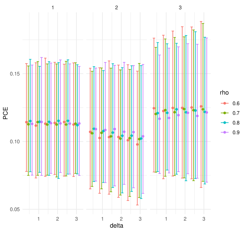
Figure 3: Posterior summaries of $PCE_{1}$, $PCE_{2}$, $PCE_{3}$ at time point $1$ for varying $\delta$ and correlation coefficients ($\rho$). X-axis: $\delta\in\{0.5,1,1.5,\dots,3\}$; Y-axis: 95% credible intervals of $PCE$s. Colored lines represent different $\rho$ values. Sensitivity parameter $\lambda_{0},\lambda_{1}$ follows a triangular prior specified in Section 4.3.

Our analysis reveals a notable pattern among the PCEs: $PCE_{3}$ exhibits the largest effect magnitude; $PCE_{2}$ shows the smallest effect size; $PCE_{1}$ falls between these two. These findings suggest that the treatment effect on HIV testing uptake is most pronounced among participants experiencing an increase in perceived social norms ($PCE_{3}$). Conversely, the subgroup with decreasing social norms ($PCE_{2}$) demonstrates the smallest treatment effect on HIV testing uptake. However, it is important to note that the 95% posterior credible intervals of the differences between these effectsinclude zero.

This pattern of results reflects an intuitive relationship between the intervention, changes in social norms, and HIV testing behavior. In particular, the stronger effect associated with increasing social norms may indicate that the intervention is particularly effective in motivating HIV testing among individuals who perceive an increment in social support and/or acceptance of testing.

6 Discussion

We have proposed an approach for inference on PCE with a continuous intermediate variable in SW-CRTs. Standard identifying assumptions include SUTVA and randomization for longitudinal designs. In addition, we propose an identification assumption that uses a copula to identify the joint distribution of the intermediate variable. We also propose a marginal structural assumption to link the unidentified conditional PCE with marginal means that can be identified from the observed data. We provide a way to calibrate the sensitivity parameters for both assumptions which exploits features of the SW-CRT design. We use our method to analyze the HIV crowdsourcing study, and found a strong associative effect, which suggests that the effect of HIV crowdsourcing intervention on units’ HIV testing behavior is the strongest within the subgroup whose social norms tend to be smaller given the intervention. In short, our method provides methodology for inference on PCE in SW-CRT and an intuitive way to calibrate the sensitivity parameters.

To the best of our knowledge, this is the first application of principal stratification framework to study the role of a continuous and repeatedly measured intermediate outcome in closed-cohort SW-CRTs. Our proposed approach can be extended in several directions. First, it is possible to further incorporate baseline covariates to relax our structural assumptions and potentially improve the statistical efficiency for estimating the principal causal effects in SW-CRTs. Second, our approach assumes ignorable dropout to handle monotone attrition of individuals. However, non-ignorable dropout may occur especially in SW-CRTs for frail populations as patients with worsened outcomes may be more likely to discontinue the study. Gasparini et al. (2024) have introduced a joint modeling approach to address a certain type of non-ignorable dropout in closed-cohort SW-CRTs in the absence of intermediate outcomes, and it would be interesting to expand that approach in our setting. Finally, we can explore relaxing the modeling assumptions in Section 4 by introducing duration-specific treatment effects (Wang et al., 2024) and/or by considering Bayesian nonparametric priors for the distribution of the observed data (Daniels et al., 2023).

Data Availability Statement

Access policies for the data set of the SW-CRT analyzed in our manuscript can be found in Tang et al. (2018) at https://doi.org/10.1371/journal.pmed.1002645.

Appendix A Equivalence of cluster-average PCE

A cluster-average type PCE estimand can be written as

$$\frac{E\left[\frac{1}{N_{j}}\sum_{i=1}^{N_{j}}\mathbb{I}\{M_{ijt}(\underline{1}_{t})=M_{ijt}(\underline{0}_{t})\}\{Y_{ijt}(\underline{1}_{t})-Y_{ijt}(\underline{0}_{t})\}\right]}{E\left[\frac{1}{N_{j}}\sum_{i=1}^{N_{j}}\mathbb{I}\{M_{ijt}(\underline{1}_{t})=M_{ijt}(\underline{0}_{t})\}\right]},$$

which is applying the definition of PCE but now restricting to a cluster-average of contrasts among this specific principal strata. Then under Assumption 4, we have

$$\qquad{E}\left\{{E}\left[\frac{1}{N_{j}}\sum_{i=1}^{N_{j}}\mathbb{I}\{M_{ijt}(\underline{1}_{t})=M_{ijt}(\underline{0}_{t})\}\{Y_{ijt}(\underline{1}_{t})-Y_{ijt}(\underline{0}_{t})\}\bigg{|}N_{j}\right]\right\}$$

$$={E}\left\{\frac{1}{N_{j}}{E}\left[\sum_{i=1}^{N_{j}}\mathbb{I}\{M_{ijt}(\underline{1}_{t})=M_{ijt}(\underline{0}_{t})\}\{Y_{ijt}(\underline{1}_{t})-Y_{ijt}(\underline{0}_{t})\}\bigg{|}N_{j}\right]\right\}$$

$$={E}\left\{\frac{N_{j}}{N_{j}}{E}\left[\mathbb{I}\{M_{ijt}(\underline{1}_{t})=M_{ijt}(\underline{0}_{t})\}\{Y_{ijt}(\underline{1}_{t})-Y_{ijt}(\underline{0}_{t})\}\bigg{|}N_{j}\right]\right\}$$

$$={E}\left\{{E}\left[\mathbb{I}\{M_{ijt}(\underline{1}_{t})=M_{ijt}(\underline{0}_{t})\}\{Y_{ijt}(\underline{1}_{t})-Y_{ijt}(\underline{0}_{t})\}\bigg{|}N_{j}\right]\right\}$$

$$={E}\left[\mathbb{I}\{M_{ijt}(\underline{1}_{t})=M_{ijt}(\underline{0}_{t})\}\{Y_{ijt}(\underline{1}_{t})-Y_{ijt}(\underline{0}_{t})\}\right]$$

$$=P\left[M_{ijt}(\underline{1}_{t})=M_{ijt}(\underline{0}_{t})\right]{E}\left[Y_{ijt}(\underline{1}_{t})-Y_{ijt}(\underline{0}_{t})\big{|}M_{ijt}(\underline{1}_{t})=M_{ijt}(\underline{0}_{t})\right]$$

Likewise,

$$E\left[\frac{1}{N_{j}}\sum_{i=1}^{N_{j}}\mathbb{I}\{M_{ijt}(\underline{1}_{t})=M_{ijt}(\underline{0}_{t})\}\right]=E\left[\mathbb{I}\{M_{ijt}(\underline{1}_{t})=M_{ijt}(\underline{0}_{t})\}\right]=P\left[M_{ijt}(\underline{1}_{t})=M_{ijt}(\underline{0}_{t})\right]$$

Hence

$$\frac{E\left[\frac{1}{N_{j}}\sum_{i=1}^{N_{j}}\mathbb{I}\{M_{ijt}(\underline{1}_{t})=M_{ijt}(\underline{0}_{t})\}\{Y_{ijt}(\underline{1}_{t})-Y_{ijt}(\underline{0}_{t})\}\right]}{E\left[\frac{1}{N_{j}}\sum_{i=1}^{N_{j}}\mathbb{I}\{M_{ijt}(\underline{1}_{t})=M_{ijt}(\underline{0}_{t})\}\right]}=P\left[Y_{ijt}(\underline{1}_{t})-Y_{ijt}(\underline{0}_{t})\big{|}M_{ijt}(\underline{1}_{t})=M_{ijt}(\underline{0}_{t})\right]$$

Appendix B Proof of Theorem 1

First,

$$\quad E(Y_{ijt}(\underline{1})-Y_{ijt}(\underline{0})|M_{ijt}(\underline{1})-M_{ijt}(\underline{0})\in\mathcal{I})$$ (12)

$$=\frac{\int_{\mathcal{I}}E(Y_{ijt}(\underline{1})-Y_{ijt}(\underline{0})|M_{ijt}(\underline{1}),M_{ijt}(\underline{0}))dP(M_{ijt}(\underline{1}),M_{ijt}(\underline{0}))}{\int_{\mathcal{I}}dP(M_{ijt}(\underline{1}),M_{ijt}(\underline{0}))}.$$

Consider the probability measure $P(M_{ijt}(\underline{1}),M_{ijt}(\underline{0}))$. By Assumption 1, 2, the marginal distribution can be identified as $P(M_{ijt}(\underline{z}))=P(M_{ijt}|\underline{Z}_{jt}=\underline{z})$. Then by Assumption 5, we have the joint distribution $P(M_{ijt}(\underline{0}),M_{ijt}(\underline{1}))$.

By Assumption 6, we can marginalize over the conditional distribution $P(M_{ijt}(\underline{1-z})|M_{ijt}(\underline{z}))$ identified by Assumption 5, and obtain the following convolution equation,

$$\qquad E(Y_{ijt}(\underline{z})|M_{ijt}(\underline{z})=m)$$

$$=\int E(Y_{ijt}(\underline{z})|M_{ijt}(\underline{1-z}),M_{ijt}(\underline{z})=m)dP(M_{ijt}(\underline{1-z})|M_{ijt}(\underline{z})=m)$$

$$=\int g^{-1}(\Delta_{ijt}(m,z)+\lambda_{z}M_{ijt}(\underline{1-z}))dP(M_{ijt}(\underline{1-z})|M_{ijt}(\underline{z})=m).$$

For the LHS, we also have

$$E(Y_{ijt}(\underline{z})|M_{ijt}(\underline{z})=m) \stackrel{{\scriptstyle\text{by Assumption 2}}}{{=}}E(Y_{ijt}(\underline{z})|M_{ijt}(\underline{z})=m,\overline{Z}_{jt}=\underline{z})$$

$$\stackrel{{\scriptstyle\text{by Assumption 1, 3}}}{{=}}E(Y_{ijt}|M_{ijt}=m,\overline{Z}_{jt}=\underline{z}).$$

Finally the convolution equation is

$$E(Y_{ijt}|M_{ijt}=m,\overline{Z}_{jt}=\underline{z}) =\int g^{-1}(\Delta_{ijt}(m,z)+\lambda_{z}M_{ijt}(\underline{1-z}))dP(M_{ijt}(\underline{1-z})|M_{ijt}(\underline{z})=m).$$ (13)

When $g$ is the identity link,

$$E(Y_{ijt}|M_{ijt}=m,\overline{Z}_{jt}=\underline{z}) =\int(\Delta_{ijt}(m,z)+\lambda_{z}M_{ijt}(\underline{1-z}))dP(M_{ijt}(\underline{1-z})|M_{ijt}(\underline{z})=m)$$

$$=\Delta_{ijt}(m,z)+\lambda_{z}E(M_{ijt}(\underline{1-z})|M_{ijt}(\underline{z})=m).$$

For a fixed $\lambda_{z}$, $\Delta_{ijt}$ is available in closed form. When $g$ is the non-identity link, $\Delta_{ijt}$ is not available in closed form, but can be solved from equation (13) using numerical integration and a Newton-Raphson algorithm.

Finally, the integrand of (12) can be identified as:

$$E(Y_{ijt}(\underline{1})|M_{ijt}(\underline{0})=m_{0},M_{ijt}(\underline{1})=m_{1}) =g^{-1}(\Delta_{ijt}(m_{1},1)+\lambda_{1}m_{0}),$$ (14)

$$E(Y_{ijt}(\underline{0})|M_{ijt}(\underline{0})=m_{0},M_{ijt}(\underline{1})=m_{1}) =g^{-1}(\Delta_{ijt}(m_{0},0)+\lambda_{0}m_{1}).$$

Appendix C Calculation of $PCE$

Recall in Theorem 1, we prove that the PCE can be identified given the assumption. In this section we show in details how to estimate the PCE in the real data analysis.

$$\quad E(Y_{ijt}(\underline{1})-Y_{ijt}(\underline{0})|M_{ijt}(\underline{1})-M_{ijt}(\underline{0})\in(a,b))$$ (15)

$$=\frac{\int_{\mathcal{I}}E(Y_{ijt}(\underline{1})-Y_{ijt}(\underline{0})|M_{ijt}(\underline{1}),M_{ijt}(\underline{0}))dP(M_{ijt}(\underline{1}),M_{ijt}(\underline{0}))}{\int_{\mathcal{I}}dP(M_{ijt}(\underline{1}),M_{ijt}(\underline{0}))}$$

C.1 Joint distribution $P(M_{ijt}(\underline{1}),M_{ijt}(\underline{0}))$

First we give the joint distribution of $M_{ijt}(\underline{0}),M_{ijt}(\underline{1})$, by (4), $M_{ijt}(\underline{z})$ follows a normal distribution, and

$$E(M_{ijt}(\underline{z})) =\eta_{1t}+\gamma_{0}+\gamma_{1}z$$

$$Var(M_{ijt}(\underline{z})) =\Sigma_{\alpha 11}+\Sigma_{\phi 11}+\sigma_{\epsilon}^{2}$$

By Assumption 5, since normal marginal distribution of both $M_{ijt}(\underline{0})$ and $M_{ijt}(\underline{1})$, Gaussian copula is bivariate normal

$$\begin{pmatrix}M_{ijt}(\underline{0})\\ M_{ijt}(\underline{1})\end{pmatrix}\sim\left(\begin{pmatrix}\eta_{1t}+\gamma_{0}\\ \eta_{1t}+\gamma_{0}+\gamma_{1}\end{pmatrix},(\Sigma_{\alpha 11}+\Sigma_{\phi 11}+\sigma_{\epsilon}^{2})\begin{pmatrix}1&\rho\\ \rho&1\end{pmatrix}\right)$$

where sensitivity parameter can be obtained in Section 4.2. Then the denominator in (15) is

$$\int_{\mathcal{I}}dP(M_{ijt}(\underline{1}),M_{ijt}(\underline{0})) =P(a\leq M_{ijt}(\underline{1})-M_{ijt}(\underline{0})<b)$$

$$=\Phi\left(\frac{b-\gamma_{1}}{\sqrt{2(1-\rho)(\Sigma_{\alpha 11}+\Sigma_{\phi 11}+\sigma_{\epsilon}^{2})}}\right)-\Phi\left(\frac{a-\gamma_{1}}{\sqrt{2(1-\rho)(\Sigma_{\alpha 11}+\Sigma_{\phi 11}+\sigma_{\epsilon}^{2})}}\right)$$

C.2 Calculation of $Y_{ijt}|M_{ijt},\underline{Z}_{jt}$

By the observed data model in Section (4), (5),

$$\left(\begin{matrix}M_{ijt}\\ \alpha_{2j}+\phi_{2ij}\end{matrix}\bigg{|}\underline{Z}_{jt}=\underline{z}\right)\sim N\left(\begin{pmatrix}\eta_{1t}+\gamma_{0}+\gamma_{1}z\\ 0\end{pmatrix},\begin{pmatrix}\sigma^{2}_{\epsilon}+\Sigma_{\alpha 11}+\Sigma_{\phi 11}&\Sigma_{\alpha 12}+\Sigma_{\phi 12}\\ \Sigma_{\alpha 12}+\Sigma_{\phi 12}&\Sigma_{\alpha 22}+\Sigma_{\phi 22}\end{pmatrix}\right)$$

Thus $\alpha_{2j}+\phi_{1j}|M_{ijt}=m,\underline{Z}_{jt}=\underline{z}$ follows a normal distribution, and

$$E(\alpha_{2j}+\phi_{2ij}|M_{ijt}=m,\underline{Z}_{jt}=\underline{z}) =\frac{\Sigma_{\alpha 12}+\Sigma_{\phi 12}}{\sigma^{2}_{\epsilon}+\Sigma_{\alpha 11}+\Sigma_{\phi 11}}(m-\eta_{1t}-\gamma_{0}-\gamma_{1}z)$$

$$Var(\alpha_{2j}+\phi_{2ij}|M_{ijt}=m,\underline{Z}_{jt}=\underline{z}) =\Sigma_{\alpha 22}+\Sigma_{\phi 22}-\frac{(\Sigma_{\alpha 12}+\Sigma_{\phi 12})^{2}}{\sigma^{2}_{\epsilon}+\Sigma_{\alpha 11}+\Sigma_{\phi 11}}$$

Then we can calculate the conditional distribution,

$$\quad E(Y_{ijt}|M_{ijt}=m,\underline{Z}_{jt}=\underline{z})$$

$$=E(\operatorname{expit}(\eta_{2t}+\beta_{0}+\beta_{1}z+\beta_{2}m+\beta_{3}mz+\alpha_{2j}+\phi_{2ij})|M_{ijt}=m)$$

$$=\sum_{k=1}^{20}w_{k}\operatorname{expit}(\eta_{2t}+\beta_{0}+\beta_{1}z+\beta_{2}m+\beta_{3}mz+s_{k})$$

where $w_{k}$ and $s_{k}$ are from implementing Gaussian-Hermite quadrature based on the conditional distribution of $\alpha_{2j}+\phi_{1j}|M_{ijt},\underline{Z}_{jt}$.

C.3 Calculation of $Y_{ijt}|M_{ijt}(0),M_{ijt}(1)$

By the observed data model in Section (4), (5), the convolution equation in (13) gives:

$$f(\Delta_{ijt}(m,z)) =-E(Y_{ijt}|M_{ijt}=m,\overline{Z}_{jt}=\underline{z})+\int\frac{e^{\Delta_{ijt}(m,z)+\lambda_{z}m^{*}}}{1+e^{\Delta_{ijt}(m,z)+\lambda_{z}m^{*}}}dP_{M_{ijt}(\underline{1-z})|M_{ijt}(\underline{z})=m}(m^{*})$$

$$=0$$

The conditional expectation $E(Y_{ijt}|M_{ijt}=m,\overline{Z}_{jt}=\underline{z})$ is calculated in Appendix C.3. We use Newton-Raphson algorithm to solve for $\Delta_{ijt}(m,z)$, the derivative is:

$$\frac{\partial f(\Delta_{ijt}(m,z))}{\partial\Delta_{ijt}(m,z)}=\int\frac{e^{\Delta_{ijt}(m,z)+\lambda_{z}m^{*}}}{(1+e^{\Delta_{ijt}(m,z)+\lambda_{z}m^{*}})^{2}}dP_{M_{ijt}(\underline{1-z})|M_{ijt}(\underline{z})=m}(m^{*}).$$

Both of the integral can be approximated by Gaussian Hermite quadrature of conditional distribution $M_{ijt}(\underline{z})|M_{ijt}(\underline{1-z})$. Once we solve $\Delta_{ijt}(m,z)$ for any $m$ and $z$, recall (14), the PCE can be calculated as follows:

$$E(Y_{ijt}(\underline{1})|M_{ijt}(\underline{0})=m_{0},M_{ijt}(\underline{1})=m_{1}) =\operatorname{expit}(\Delta_{ijt}(m_{1},1)+\lambda_{1}m_{0}),$$

$$E(Y_{ijt}(\underline{0})|M_{ijt}(\underline{0})=m_{0},M_{ijt}(\underline{1})=m_{1}) =\operatorname{expit}(\Delta_{ijt}(m_{0},0)+\lambda_{0}m_{1}).$$

We the use Monte Carlo to calculate the numerator in (15) by sampling from the truncated joint distribution of $(M_{ijt}(\underline{0}),M_{ijt}(\underline{1}))$

$$\int_{\mathcal{I}}E(Y_{ijt}(\underline{1})-Y_{ijt}(\underline{0})|M_{ijt}(\underline{1}),M_{ijt}(\underline{0}))dP(M_{ijt}(\underline{1}),M_{ijt}(\underline{0}))$$

$$= \sum_{i}E(Y_{ijt}(\underline{1})-Y_{ijt}(\underline{0})|M_{ijt}(\underline{1})=m_{i1},M_{ijt}(\underline{0})=m_{i0})I((m_{i1},m_{i0})\in\mathcal{I})$$

where $m_{i0},m_{i1}$ are sampled from the joint distribution.

Appendix D Calculation of calibrated $\rho^{*}$

Let $\mathcal{C}=\{(i,j,t):Z_{j,t-1}=0,Z_{jt}=1\}$ denote the set of observations satisfying the conditions $Z_{j,t-1}=0$ and $Z_{jt}=1$. For time-varying $\rho^{*}_{\tau}$, we define the subset $\mathcal{C}_{\tau}=\{(i,j,t):t=\tau,Z_{j,t-1}=0,Z_{jt}=1\}$. Under SUTVA, the covariance and variance can be estimated as follows:

$$\widehat{\text{Var}}(M_{ij,t-1}(\underline{0})) =\frac{1}{|\mathcal{C}|-1}\sum_{(i,j,t)\in\mathcal{C}}(M_{ij,t-1}-\widehat{\mu}_{0})^{2}$$

$$\widehat{\text{Var}}(M_{ijt}(\underline{1})) =\frac{1}{|\mathcal{C}|-1}\sum_{(i,j,t)\in\mathcal{C}}(M_{ijt}-\widehat{\mu}_{1})^{2}$$

$$\widehat{\text{Cov}}(M_{ij,t-1}(\underline{0}),M_{ijt}(\underline{1})) =\frac{1}{|\mathcal{C}|-1}\sum_{(i,j,t)\in\mathcal{C}}(M_{ij,t-1}-\widehat{\mu}_{0})(M_{ijt}-\widehat{\mu}_{1})$$

where $\widehat{\mu}_{0}=\frac{1}{|\mathcal{C}|}\sum_{(i,j,t)\in\mathcal{C}}M_{ij,t-1}$, $\widehat{\mu}_{1}=\frac{1}{|\mathcal{C}|}\sum_{(i,j,t)\in\mathcal{C}}M_{ijt}$. For time-varying $\rho^{*}$, the variance and covariance are calculated in a smaller set, which are:

$$\widehat{\text{Var}}(M_{ij,t-1}(\underline{0})) =\frac{1}{|\mathcal{C}_{t}|-1}\sum_{(i,j,t)\in\mathcal{C}_{t}}(M_{ij,t-1}-\widehat{\mu}_{0})^{2}$$

$$\widehat{\text{Var}}(M_{ijt}(\underline{1})) =\frac{1}{|\mathcal{C}_{t}|-1}\sum_{(i,j,t)\in\mathcal{C}_{t}}(M_{ijt}-\widehat{\mu}_{1})^{2}$$

$$\widehat{\text{Cov}}(M_{ij,t-1}(\underline{0}),M_{ijt}(\underline{1})) =\frac{1}{|\mathcal{C}_{t}|-1}\sum_{(i,j,t)\in\mathcal{C}_{t}}(M_{ij,t-1}-\widehat{\mu}_{0})(M_{ijt}-\widehat{\mu}_{1})$$

where $\widehat{\mu}_{0}=\frac{1}{|\mathcal{C}_{t}|}\sum_{(i,j,t)\in\mathcal{C}_{t}}M_{ij,t-1}$, $\widehat{\mu}_{1}=\frac{1}{|\mathcal{C}_{t}|}\sum_{(i,j,t)\in\mathcal{C}_{t}}M_{ijt}$.

Appendix E Priors

The priors for fixed effect parameters are set as follows:

$$\beta_{1},\beta_{2},\beta_{3},\beta_{4} \sim N(0,10)$$

$$\gamma_{0},\gamma 1 \sim N(0,10)$$

$$\eta_{1t},\eta_{2t} \sim N(0,10),\ t=1,2,3,4$$

The priors for random effect parameters are set as follows:

$$\sigma_{\epsilon} \sim\text{Exponential}(1)$$

$$\sigma_{\alpha 1},\sigma_{\alpha 2} \sim\text{Exponential}(1)$$

$$\sigma_{\phi 1},\sigma_{\phi 2} \sim\text{Exponential}(1)$$

$$\rho_{\alpha} \sim\text{Uniform}(-1,1)$$

$$\rho_{\phi} \sim\text{Uniform}(-1,1)$$

Here we model the covariance matrix $\Sigma_{\alpha}$, $\Sigma_{\phi}$ in this way for more efficient and stable sampling.

References

- Angrist et al. (1996) Angrist, J. D., Imbens, G. W., and Rubin, D. B. (1996). Identification of causal effects using instrumental variables. Journal of the American Statistical Association 91, 444–455.
- Antonelli et al. (2023) Antonelli, J., Mealli, F., Beck, B., and Mattei, A. (2023). Principal stratification with continuous treatments and continuous post-treatment variables.
- Athey and Imbens (2022) Athey, S. and Imbens, G. W. (2022). Design-based analysis in difference-in-differences settings with staggered adoption. Journal of Econometrics 226, 62–79.
- Babalola (2007) Babalola, S. (2007). Readiness for hiv testing among young people in northern nigeria: The roles of social norm and perceived stigma. AIDS and behavior 11, 759–69.
- Baccini et al. (2017) Baccini, M., Mattei, A., and Mealli, F. (2017). Bayesian inference for causal mechanisms with application to a randomized study for postoperative pain control. Biostatistics 18, 605–617.
- Bartolucci and Grilli (2011) Bartolucci, F. and Grilli, L. (2011). Modeling partial compliance through copulas in a principal stratification framework. Journal of the American Statistical Association 106, 469–479.
- Carpenter et al. (2017) Carpenter, B., Gelman, A., Hoffman, M. D., Lee, D., Goodrich, B., Betancourt, M., Brubaker, M., Guo, J., Li, P., and Riddell, A. (2017). Stan : A Probabilistic Programming Language. Journal of Statistical Software 76,.
- Chen and Li (2024) Chen, X. and Li, F. (2024). Model-assisted analysis of covariance estimators for stepped wedge cluster randomized experiments. Scandinavian Journal of Statistics pages 1–31.
- Dai et al. (2012) Dai, J. Y., Gilbert, P. B., and Mâsse, B. R. (2012). Partially hidden markov model for time-varying principal stratification in hiv prevention trials. Journal of the American Statistical Association 107, 52–65.
- Daniels et al. (2023) Daniels, M. J., Linero, A., and Roy, J. (2023). Bayesian nonparametrics for causal inference and missing data. CRC Press.
- Daniels et al. (2012) Daniels, M. J., Roy, J. A., Kim, C., Hogan, J. W., and Perri, M. G. (2012). Bayesian inference for the causal effect of mediation. Biometrics 68, 1028–1036.
- Ding and Lu (2017) Ding, P. and Lu, J. (2017). Principal stratification analysis using principal scores. Journal of the Royal Statistical Society Series B: Statistical Methodology 79, 757–777.
- Efron and Feldman (1991) Efron, B. and Feldman, D. (1991). Compliance as an explanatory variable in clinical trials. Journal of the American Statistical Association 86, 9–17.
- Frangakis et al. (2004) Frangakis, C. E., Brookmeyer, R. S., Varadhan, R., Safaeian, M., Vlahov, D., and Strathdee, S. A. (2004). Methodology for evaluating a partially controlled longitudinal treatment using principal stratification, with application to a needle exchange program. Journal of the American Statistical Association 99, 239–249.
- Frangakis and Rubin (2002) Frangakis, C. E. and Rubin, D. B. (2002). Principal stratification in causal inference. Biometrics 58, 21–29.
- Frumento et al. (2012) Frumento, P., Mealli, F., Pacini, B., and Rubin, D. B. (2012). Evaluating the effect of training on wages in the presence of noncompliance, nonemployment, and missing outcome data. Journal of the American Statistical Association 107, 450–466.
- Gasparini et al. (2024) Gasparini, A., Crowther, M. J., Hoogendijk, E. O., Li, F., and Harhay, M. O. (2024). Analysis of cohort stepped wedge cluster-randomized trials with non-ignorable dropout via joint modeling. arXiv preprint arXiv:2404.14840 .
- Heagerty (1999) Heagerty, P. J. (1999). Marginally specified logistic-normal models for longitudinal binary data. Biometrics 55, 688–698.
- Hemming and Taljaard (2020) Hemming, K. and Taljaard, M. (2020). Reflection on modern methods: When is a stepped-wedge cluster randomized trial a good study design choice? International Journal of Epidemiology 49, 1043–1052.
- Hussey and Hughes (2007) Hussey, M. A. and Hughes, J. P. (2007). Design and analysis of stepped wedge cluster randomized trials. Contemporary Clinical Trials 28, 182–191.
- Imai et al. (2010) Imai, K., Keele, L., and Yamamoto, T. (2010). Identification, inference and sensitivity analysis for causal mediation effects. Statistical Science 25, 51–71.
- Imbens and Rubin (1997) Imbens, G. W. and Rubin, D. B. (1997). Bayesian inference for causal effects in randomized experiments with noncompliance. The Annals of Statistics 25,.
- Jin and Rubin (2008) Jin, H. and Rubin, D. B. (2008). Principal stratification for causal inference with extended partial compliance. Journal of the American Statistical Association 103, 101–111.
- Kahan et al. (2024) Kahan, B. C., Blette, B. S., Harhay, M. O., Halpern, S. D., Jairath, V., Copas, A., and Li, F. (2024). Demystifying estimands in cluster-randomised trials. Statistical Methods in Medical Research 33, 1211–1232.
- Kenny et al. (2022) Kenny, A., Voldal, E. C., Xia, F., Heagerty, P. J., and Hughes, J. P. (2022). Analysis of stepped wedge cluster randomized trials in the presence of a time-varying treatment effect. Statistics in Medicine 41, 4311–4339.
- Kim et al. (2019) Kim, C., Daniels, M. J., Hogan, J. W., Choirat, C., and Zigler, C. M. (2019). Bayesian methods for multiple mediators: Relating principal stratification and causal mediation in the analysis of power plant emission controls. The annals of applied statistics 13, 1927–1956.
- Li et al. (2021) Li, F., Hughes, J. P., Hemming, K., Taljaard, M., Melnick, E. R., and Heagerty, P. J. (2021). Mixed-effects models for the design and analysis of stepped wedge cluster randomized trials: An overview. Statistical Methods in Medical Research 30, 612–639.
- Lin et al. (2008) Lin, J. Y., Ten Have, T. R., and Elliott, M. R. (2008). Longitudinal nested compliance class model in the presence of time-varying noncompliance. Journal of the American Statistical Association 103, 462–473.
- Lin et al. (2009) Lin, J. Y., Ten Have, T. R., and Elliott, M. R. (2009). Nested markov compliance class model in the presence of time-varying noncompliance. Biometrics 65, 505–513.
- Magnusson et al. (2019) Magnusson, B. P., Schmidli, H., Rouyrre, N., and Scharfstein, D. O. (2019). Bayesian inference for a principal stratum estimand to assess the treatment effect in a subgroup characterized by postrandomization event occurrence. Statistics in Medicine 38, 4761–4771.
- Maleyeff et al. (2023) Maleyeff, L., Li, F., Haneuse, S., and Wang, R. (2023). Assessing exposure-time treatment effect heterogeneity in stepped-wedge cluster randomized trials. Biometrics 79, 2551–2564.
- Neal (2011) Neal, R. M. (2011). Mcmc using hamiltonian dynamics. Handbook of Markov Chain Monte Carlo 2,.
- Nevins et al. (2024) Nevins, P., Ryan, M., Davis-Plourde, K., Ouyang, Y., Pereira Macedo, J. A., Meng, C., Tong, G., Wang, X., Ortiz-Reyes, L., Caille, A., et al. (2024). Adherence to key recommendations for design and analysis of stepped-wedge cluster randomized trials: A review of trials published 2016–2022. Clinical Trials 21, 199–210.
- Nevo and Gorfine (2022) Nevo, D. and Gorfine, M. (2022). Causal inference for semi-competing risks data. Biostatistics 23, 1115–1132.
- Perkins et al. (2018) Perkins, J. M., Nyakato, V. N., Kakuhikire, B., Mbabazi, P. K., Perkins, H. W., Tsai, A. C., Subramanian, S. V., Christakis, N. A., and Bangsberg, D. R. (2018). Actual vs. perceived hiv testing norms, and personal hiv testing uptake: A cross-sectional, population-based study in rural uganda. AIDS and behavior 22, 616–628.
- Roy et al. (2008) Roy, J., Hogan, J. W., and Marcus, B. H. (2008). Principal stratification with predictors of compliance for randomized trials with 2 active treatments. Biostatistics 9, 277–289.
- Rubin (1974) Rubin, D. B. (1974). Estimating causal effects of treatments in randomized and nonrandomized studies. Journal of Educational Psychology 66, 688–701.
- Rubin (1980) Rubin, D. B. (1980). Randomization analysis of experimental data: The fisher randomization test comment. Journal of the American Statistical Association 75, 591–593.
- Schwartz et al. (2011) Schwartz, S. L., Li, F., and Mealli, F. (2011). A bayesian semiparametric approach to intermediate variables in causal inference. Journal of the American Statistical Association 106, 1331–1344.
- Tang et al. (2018) Tang, W., Wei, C., Cao, B., Wu, D., Li, K. T., Lu, H., Ma, W., Kang, D., Li, H., Liao, M., Mollan, K. R., Hudgens, M. G., Liu, C., Huang, W., Liu, A., Zhang, Y., Smith, M. K., Mitchell, K. M., Ong, J. J., Fu, H., Vickerman, P., Yang, L., Wang, C., Zheng, H., Yang, B., and Tucker, J. D. (2018). Crowdsourcing to expand hiv testing among men who have sex with men in china: A closed cohort stepped wedge cluster randomized controlled trial. PLOS Medicine 15, e1002645.
- VanderWeele (2008) VanderWeele, T. J. (2008). Simple relations between principal stratification and direct and indirect effects. Statistics & Probability Letters 78, 2957–2962.
- Wang et al. (2024) Wang, B., Wang, X., and Li, F. (2024). How to achieve model-robust inference in stepped wedge trials with model-based methods? Biometrics pages 1–25.
- Xu et al. (2022) Xu, Y., Scharfstein, D., Müller, P., and Daniels, M. (2022). A Bayesian nonparametric approach for evaluating the causal effect of treatment in randomized trials with semi-competing risks. Biostatistics 23, 34–49.
- Yau and Little (2001) Yau, L. H. Y. and Little, R. J. (2001). Inference for the complier-average causal effect from longitudinal data subject to noncompliance and missing data, with application to a job training assessment for the unemployed. Journal of the American Statistical Association 96, 1232–1244.
- Zhang et al. (2009) Zhang, J. L., Rubin, D. B., and Mealli, F. (2009). Likelihood-based analysis of causal effects of job-training programs using principal stratification. Journal of the American Statistical Association 104, 166–176.
- Zhao et al. (2018) Zhao, P., Liu, L., Zhang, Y., Cheng, H., Cao, B., Liu, C., Wang, C., Yang, B., Wei, C., Tucker, J. D., and Tang, W. (2018). The interaction between hiv testing social norms and self-efficacy on hiv testing among chinese men who have sex with men: Results from an online cross-sectional study. BMC infectious diseases 18, 541.
- Zigler et al. (2012) Zigler, C. M., Dominici, F., and Wang, Y. (2012). Estimating causal effects of air quality regulations using principal stratification for spatially correlated multivariate intermediate outcomes. Biostatistics 13, 289–302.