Floquet driven long-range interactions induce super-extensive scaling in quantum battery

Abstract

Achieving quantum advantage in energy storage and power extraction is a primary objective in the design of quantum-based batteries. We explore how long-range (LR) interactions in conjunction with Floquet driving can improve the performance of quantum batteries, particularly when the battery is initialized in a fully polarized state. In particular, we exhibit that by optimizing the driving frequency, the maximum average power scales super extensively with system-size which is not achievable through next-nearest neighbor interactions or traditional unitary charging, thereby gaining genuine quantum advantage. We illustrate that the inclusion of either two-body or many-body interaction terms in the LR charging Hamiltonian leads to a scaling benefit. Furthermore, we discover that a super-linear scaling in power results from increasing the strength of interaction compared to the transverse magnetic field and the range of interaction with low fall-off rate, highlighting the advantageous role of long-range interactions in optimizing quantum battery charging.

I Introduction

The development and miniaturization of technology in the modern day have led to the creation of quantum thermal devices, such as batteries Alicki and Fannes (2013); Campaioli et al. (2018, 2024), refrigerators Linden et al. (2010), transistors Joulain et al. (2016), and heat engines Bender et al. (2000); Quan et al. (2007), which can outperform their classical counterparts by leveraging quantum mechanical principles. In addition to their technological implications, these studies of quantum thermal devices contribute to advancing thermodynamic concepts in the microscopic and nanoscale regimes Gemmer et al. (2004).

In this work, we will focus on the benefits of developing batteries based on quantum mechanics, composed of quantum states that store and extract energy. One key factor of quantum batteries (QB) is the use of collective operations during the charging process. These operations can generate quantum correlations or other forms of quantumness that lead to super-extensive scaling of power (meaning that the power output increases super-linearly with the number of cells in the battery) Gyhm et al. (2022); Campaioli et al. (2024), known as genuine quantum advantage Andolina et al. (2024). On the other hand, the quantum interacting spin models as quantum batteries have been shown to offer advantages over non-interacting models in generating power since the latter cannot create quantum correlations in the system Le et al. (2018); Ghosh et al. (2020, 2021); Ghosh and Sen (De). However, it is necessary to note that not all collective interactions yield a genuine quantum advantage; rather, only when the norm of charging Hamiltonian increases super-extensively with system size Gyhm et al. (2022); Julià-Farré et al. (2020). Since the concept of QBs was first proposed Alicki and Fannes (2013), several theoretical protocols have been developed to explore their performance, highlighting how quantum mechanical phenomena Ferraro et al. (2018); Andolina et al. (2019); Santos et al. (2019); Rossini et al. (2020); Julià-Farré et al. (2020); Sen and Sen (2021); Crescente et al. (2020, 2022); Konar et al. (2022, 2024a, 2024b); Chaki et al. (2024); Arjmandi et al. (2022); Santos et al. (2023); Chaki et al. (2023); Rodríguez et al. (2023); Mitra and Srivastava (2024a); Yan and Jing (2023); Song et al. (2024); Lu et al. (2024); Niu et al. (2024); Mitra and Srivastava (2024b); Perciavalle et al. (2024) — such as indefinite causal order Zhu et al. (2023) and many-body localization Rossini et al. (2019); Arjmandi et al. (2023) — can improve energy storage. These ideas have been demonstrated in various physical systems, including quantum dots de Buy Wenniger et al. (2023), transmons Dou and Yang (2023); Hu et al. (2022); Gemme et al. (2022), organic semiconductors Quach et al. (2022), and nuclear magnetic resonance Joshi and Mahesh (2022).

Our primary goal here is to enhance the performance of the quantum batteries by involving Floquet driving and long-range (LR) interactions into the charging process. In recent years, Floquet or time-periodic driving, also referred to as Floquet engineering, has emerged as a vital tool for exploring unique characteristics in many-body systems that are typically inaccessible in equilibrium conditions (for details, see reviews Bukov et al. (2015); Eckardt and Anisimovas (2015); Mori (2023)). Notable examples include topological order Bukov et al. (2015), prethermalization region Eckardt and Anisimovas (2015); McRoberts et al. (2023), dynamical localization and stabilization D’Alessio et al. (2016) and the creation of artificial magnetic fields Bloch et al. (2008); Aidelsburger et al. (2013).

Furthermore, periodic driving can be easily implemented via oscillating electromagnetic radiation in experiments with cold atoms in optical lattices Eckardt and Anisimovas (2015); Eckardt (2017) and solid state materials, thereby paving the way to the creation of systems with unique characteristics. Hence, it is natural to apply Floquet evolution towards building quantum technologies including quantum communication Engelhardt et al. (2024), quantum computing Fauseweh and Zhu (2023), quantum refrigerator Kolisnyk et al. (2024), quantum transistor Gupt et al. (2022), heat engine Niedenzu et al. (2015); Niedenzu and Kurizki (2018), and most recently quantum batteries Mondal and Bhattacharjee (2022). In the case of QB, it was shown that although the effective periodic charging involves collective operations, it does not lead to super-extensive scaling of power Mondal and Bhattacharjee (2022).

We exhibit that this shortfall of Floquet charging in QB may be overcome by introducing long-range interactions. This approach expands the scope of benefits associated with LR spin models for various quantum information processing tasks, including quantum sensing and computation Koffel et al. (2012); Vodola et al. (2014); Mahto et al. (2022); Monika et al. (2023); Ghosh et al. (2024). A primary advantage in terms of implementability is that LR interactions arise naturally in experiments with trapped ions and cold-atoms. At the same time, Floquet driving can also be implemented in these physical systems Eckardt (2017); Wang et al. (2017); Olmschenk et al. (2007); He et al. (2021). To explore this, we begin with the initial product eigenstate of a non-interacting battery Hamiltonian and consider two types of LR $XY$ spin models for charging, where the interaction range follows a power-law decay. One of these models involves two-body long-range interacting term while the other one contains many-body LR interactions. Notably, the latter can be solved analytically via Jordan-Wigner transformation Lieb et al. (1961); Barouch et al. (1970); Barouch and McCoy (1971); Vodola et al. (2014, 2015); Sadhukhan et al. (2020); Jaschke et al. (2017); Lakkaraju et al. (2022) while the former one can be handled numerically except for the special case corresponding to the Lipkin Meshkov Glick (LMG) model Lipkin et al. (1965).

We illustrate analytically and numerically that while the battery’s power can be increased by competing next-nearest neighbor (NNN) interactions with nearest-neighbor (NN) ones, super-linear scaling cannot be attained, thereby indicating the deficiency in short-range interactions. We further exhibit that LR interactions, combined with periodic driving, can lead to super-linear scaling, provided that the strengths of the magnetic field and the LR interactions are appropriately calibrated, known as genuine quantum advantage Andolina et al. (2024). In order to establish this, we adopt the definition of the maximum average power of the QB in which the optimization is performed over the stroboscopic time and the frequency of the Floquet charging. We discover that super-linear scaling can be accomplished for both kinds of LR interactions when the coordination number is close to its maximum and the fall-off rate of interactions is low enough to provide truly long-range.

The paper is organized in the following manner. Sec. II introduces the set-up of the quantum battery including LR charging Hamiltonian, its Floquet charging set-up and the benefits of additional NNN interactions with NN interactions in charging Hamiltonian. The super-extensive scaling of QB is reported for LR $XY$ model in Sec. III. The performance of QB with the extended $XY$ model which can be solved analytically is presented in Sec. IV. Sec. V includes the concluding remarks.

II Interplay between nearest-neighbor and next-nearest neighbor interactions with Floquet charging

We establish here that although short-range interaction can be beneficial to enhance the power of the QB, super-extensive scaling can only be attained with LR interactions. More precisely, we focus here on the trade-off relation between nearest-neighbor and next-nearest neighbor interaction strengths present in the charging Hamiltonian which also depends on the stroboscopic time. Before presenting the results, let us fix the set-up for quantum battery under consideration.

Set-up for quantum battery: Protocol of Floquet charging

Quantum battery. We prepare the initial state of the quantum battery as a thermal equilibrium state, $\rho(0)=\exp(-\beta H_{B})/\text{Tr}(\exp(-\beta H_{B}))$ where $\beta=1/k_{B}T$ with $k_{B}$ being the Boltzmann constant and $T$ representing the temperature. We choose the battery Hamiltonian to be $H_{B}=h_{z}\sum_{j}\sigma^{z}_{j}$, where $h_{z}$ is the strength of the local magnetic field, quantifying the local energy gap of each subsystem and $\sigma^{z}$ is the $z$-component of the Pauli matrix. Note that when $\beta\to\infty$, $\rho(0)$ reaches to the ground state of $H_{B}$, i.e., $\ket{\psi(t=0)}=\ket{00\ldots 0}$ with $\ket{0}$ being the ground state of $\sigma^{z}$.

Charging the battery. In order to obtain super-linear scaling of QB, we will demonstrate that the charging operation plays an important role. We incorporate two important components in the charging Hamiltonian of the QB, $H_{ch}(t)=H_{B}+H_{int}(t)$, which are different from the previous protocols known in the literature Bera et al. (2019); Mondal and Bhattacharjee (2022). These two crucial ingredients are as follows:
(1a) We choose variable-range interacting Hamiltonian as $H_{int}$, given by

$$H_{int}^{LR}=\sum_{\begin{subarray}{c}i<j\\ |i-j|\leq Z\end{subarray}}^{N-Z}{\frac{J(t)}{\mathcal{N}|i-j|^{\alpha}}(\sigma_{i}^{x}\sigma_{j}^{x}}+\gamma\sigma_{i}^{y}\sigma_{j}^{y}),$$ (1)

which is responsible to build a multi-site correlation between different subsystems of the QB. Here $J(t)$ is the time-dependent interaction strength between the spins at site, $i$ and $j$ with $\mathcal{N}=\sum_{r=1}^{Z}\frac{1}{r^{\alpha}},\,r=|i-j|$, known as the Kac normalization factor Kac et al. (1963), $\gamma$ and $Z$ represent the anisotropic factor and the coordination number, i.e., the distance between sites, $i$ and $j$ respectively and $\sigma^{k}$ ($k=x,y,z$) are the Pauli matrices. We also assume a power-law functional form for the decay of the interactions with the increasing distance between the spins such that $\alpha$ corresponds to the fall-off rate of this power law-decay. In this case, an open-boundary is considered. By changing $\alpha$ values, we can have long-range interactions with $0\leq\alpha\leq 1$, quasi LR interactions for $1<\alpha\leq 2$ and short-range interaction when $\alpha>2$. Note that $\alpha=0$ corresponds to the LMG model Lipkin et al. (1965). In this work, we study the gain in QB by varying both $\alpha$ and $Z$.
(1b) Another model that we choose for charging is the extended $XY$ model which can be solved analytically by Jordan-Wigner transformation Lieb et al. (1961); Barouch et al. (1970); Barouch and McCoy (1971). In this case, the interacting Hamiltonian reads as

$$H_{int}^{exXY}=\sum_{j=1}^{N}\sum_{r=1}^{\frac{N}{2}}\frac{J(t)}{4\mathcal{N}r^{\alpha}}(\sigma_{j}^{x}\mathbb{Z}_{r}^{z}\sigma_{j+r}^{x}+\gamma\sigma_{j}^{y}\mathbb{Z}_{r}^{z}\sigma_{j+r}^{y}),$$ (2)

where $\mathbb{Z}_{r}^{z}=\prod_{l=j+1}^{j+r-1}\sigma_{l}^{z}$, with $\mathbb{Z}_{1}^{z}=\mathbb{I}$, with $\alpha$ being the strength of power-law decay and the Kac-scaling factor respectively as given in Eq. (1). Here a periodic boundary condition is considered. We are interested to find out whether the extended $XY$ model in Eq. (2) involving both $N$-body interactions and long-range interactions can provide similar or any additional benefit compared to the long-range models in Eq. (1).

(2) We consider the evolution of QB through square wave with time period, $T=\frac{2\pi}{\omega}$, given as

$$J(t)=\begin{cases}+J;&nT<t<(n+1/2)T\\ -J;&(n+1/2)T<t<nT,\\ \end{cases}$$ (3)

where $\omega$ represents the frequency of the periodic driving. Given the square wave form of the periodic drive performed at stroboscopic times, we use the unitary of the form

$$U_{1}=\exp[-i(H_{B}+H_{int})\frac{T}{2}],\,U_{2}=\exp[-i(H_{B}-H_{int})\frac{T}{2}],$$

$$U^{F}(T)=U_{2}U_{1},$$ (4)

where $U^{F}$ is unitary corresponding to the periodic time, $T$. The $n^{th}$ stroboscopic evolution from the initial state, $\ket{\psi(t=0)}$, is given as $\ket{\psi(t=nT)}=(U^{F})^{n}\ket{\psi(t=0)}$.

Performance quantifier. In order to certify the performance of the battery with respect to its capability in storing and extractable energy, we compute the work stored in a given battery at each stroboscopic time, $nT$, as $W(t=nT)=\Tr(H_{B}\rho(t))-\Tr(H_{B}\rho(0))$, where $\rho(0)$ and $\rho(t)$ are the initial and the evolved state of the battery. Since changing certain parameters of the Hamiltonian can cause extraction of more power, making the design unreasonable, we normalize the Hamiltonian. It makes its spectrum to be bounded by $[~-1,1]$, irrespective of any system parameters which is given as $(E_{max}-E_{min})^{-1}[2H_{B}-(E_{max}+E_{min})\mathbb{I}]\rightarrow H_{B}$.

We are interested to investigate the maximum average power of the battery at each stroboscopic time, given by

$$P_{max}^{\omega}=\underset{n,\omega}{\max}\quad\frac{W(nT)}{nT},$$ (5)

where the maximization is performed over stroboscopic time, $t$ and the frequency range, $\omega$. Note that the optimization over $\omega$ does not appear in the unitary evolution and is not considered for Floquet charging in literature (see Ref. Mondal and Bhattacharjee (2022)). Further, when $\omega\to 0$, the system evolves unitarily and the time period is very high for which power through stroboscopic time become very small, i.e., $P_{max}\to 0$ while for $\omega\to\infty$, QB evolves through an average Hamiltonian $H_{B}$ resulting in $P_{max}\to 0$. Therefore, it highlights that nonvanishing maximum power depends upon $\omega$ and genuine quantum advantage through Floquet charging can only be confirmed through optimization over frequency as well as stroboscopic time. In other words, we are interested to identify the favorable situation in which quantum advantage can be maximized as done in case of other quantum tasks Nielsen and Chuang (2000); Giovannetti et al. (2006); De and Sen (2011); Gisin and Thew (2007). Note here that the normalization of the battery Hamiltonian $H_{B}$ described above is not performed when we compute the scaling behavior of $P_{max}^{\omega}$ with the system-size $N$ since we want to compare our results with the known results in literature computed without normalization.

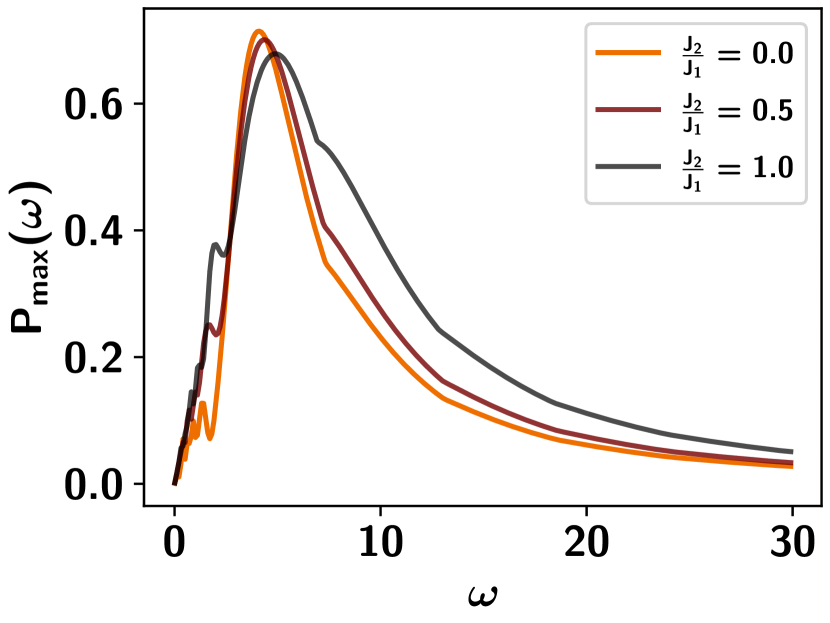
Figure 1: Behavior of $P_{\max}(\omega)$ (ordinate) against $\omega$ (abscissa) of the $XY$ model with the increase of $J_{2}/J_{1}$ (from dark to light lines). Here $h_{z}=0.5$, $\gamma=-1$ and $N=8$. The initial state is the product ground state of the battery Hamiltonian, $H_{B}=h_{z}\sum_{j}\sigma^{z}_{j}$. We observe that there exists $\omega$ values for which $P_{\max}(\omega)$ attain its maximum. Both the axes are dimensionless.

II.1 Advantage of having NN and NNN interactions though no super-linear scaling

Before moving to the charging with LR interactions (i.e., with arbitrary $\alpha$ and arbitrary $Z$), let us first analyze whether along with nearest-neighbor interactions, denoted by $J_{1}$, if one incorporates next-nearest neighbor interaction with $J_{2}$ in the charging Hamiltonian (i.e., $\alpha=0$ and $Z=2$ in Eq. (1)), any enhancement of power can be achieved or not. The Hamiltonian can be written explicitly as

$$H_{int}^{NNN} = \sum_{\begin{subarray}{c}i=1\end{subarray}}^{N-1}{\frac{J_{1}(t)}{2}(\sigma_{i}^{x}\sigma_{i+1}^{x}}+\gamma\sigma_{i}^{y}\sigma_{i+1}^{y})$$ (6)

$$+ \sum_{\begin{subarray}{c}i=1\end{subarray}}^{N-2}{\frac{J_{2}(t)}{2}(\sigma_{i}^{x}\sigma_{i+2}^{x}}+\gamma\sigma_{i}^{y}\sigma_{i+2}^{y}),$$

To address this query, we choose two paths – (1) we study $P_{\max}(\omega)=\underset{n}{\max}\quad\frac{W(nT)}{nT}$ by varying the strength of $J_{2}/J_{1}$ for a fixed $\omega$ and the same with the increase of $\omega$ for different values of $J_{2}/J_{1}$; (2) secondly, for a large values of $\omega$, we apply Floquet-Magnus expansion Blanes et al. (2009) and study the scaling behavior of this model with $N$ for various $J_{2}/J_{1}$ strength and try to see whether we can beat linear scaling obtained for NN interacting charging.

II.1.1 Gain in power with NNN interacting charger

We first note that power can be enhanced when charging Hamiltonian contains any kinds of interactions, thereby confirming the role of quantumness for storing energy in the battery. In case of Floquet charging, another crucial component is the frequency. To determine the role of $\omega$ and the interaction strengths, we investigate the behavior of $P_{\max}(\omega,J_{2}/J_{1},h_{z})$ where $J_{2}/J_{1}$ and $h_{z}$ are system parameters of the QB and charger respectively. Since we are interested to explore the role NNN interactions in charging, we fix $h_{z}$ to be moderately low compared to the interaction strength.

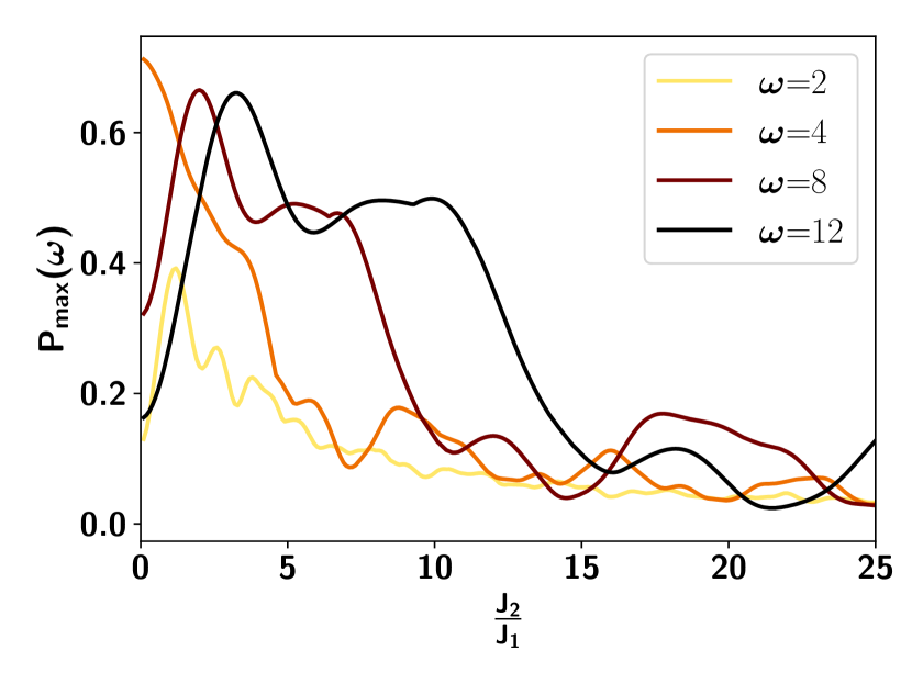
Figure 2: $P_{\max}(\omega)$ (ordinate) with respect to $\frac{J_{2}}{J_{1}}$ (abscissa) of the $XY$ model with the increase of the frequency of the periodic driving, $\omega$ (from light to dark lines). All the system parameters are same as in Fig. 1. Clearly, there exists $\omega_{c}$ above which NNN interaction combined with NN ones provides advantage over the charging Hamiltonian with only NN interactions. Both the axes are dimensionless.

Observation 1. The entire profile of $P_{\max}(\omega,J_{2}/J_{1})$ depends crucially on $\omega$ (see Fig. 1), showing the importance of frequency in the Floquet driving. It is evident from the investigation that for a fixed system parameters, the maximum of $P_{\max}(\omega)$ is achieved only for a single value of $\omega$.

Observation 2. $P_{\max}(\omega,J_{2}/J_{1})$ oscillates non-uniformly with the variation of $J_{2}/J_{1}$ for a fixed $\omega$ value although it saturates when $J_{2}/J_{1}$ is moderately high. In particular, for some values of $\omega$, there exist a range of $J_{2}/J_{1}$ for which $P_{\max}(\omega,J_{2}/J_{1})\geq P_{\max}(\omega,J_{2}/J_{1}=0)$, thereby illustrating the benefit of NNN interactions in charging. However, the increasing value of $J_{2}$ over $J_{1}$ is not ubiquitously beneficial as depicted in Fig. 2. It only highlights that the competition between NN and NNN interactions matters in storing energy. This observation also justifies the importance of maximizing $\omega$ for studying the power of the QB.

Observation 3. Let us consider the maximum stored energy with stroboscopic time, given by $W_{\max}(J_{2}/J_{1},h_{z})=\underset{n}{\max}\quad W(nT)$ which reaches maximum for some $\omega$ values when the system parameters are fixed. The $\omega$ for which $W_{\max}$ achieves maximum changes with the ratio between the NN and NNN interactions for a weak magnetic field strength. Interestingly, we observe that with the increasing $J_{2}/J_{1}$, $W_{\max}$ increases with $\omega$ and as shown for $P_{\max}({\omega},J_{2}/J_{1})$, there exists $\omega_{c}$ for a fixed $J_{2}/J_{1}$ which leads to the maximum of $W_{\max}$.

II.1.2 No benefit in scaling with NNN interactions

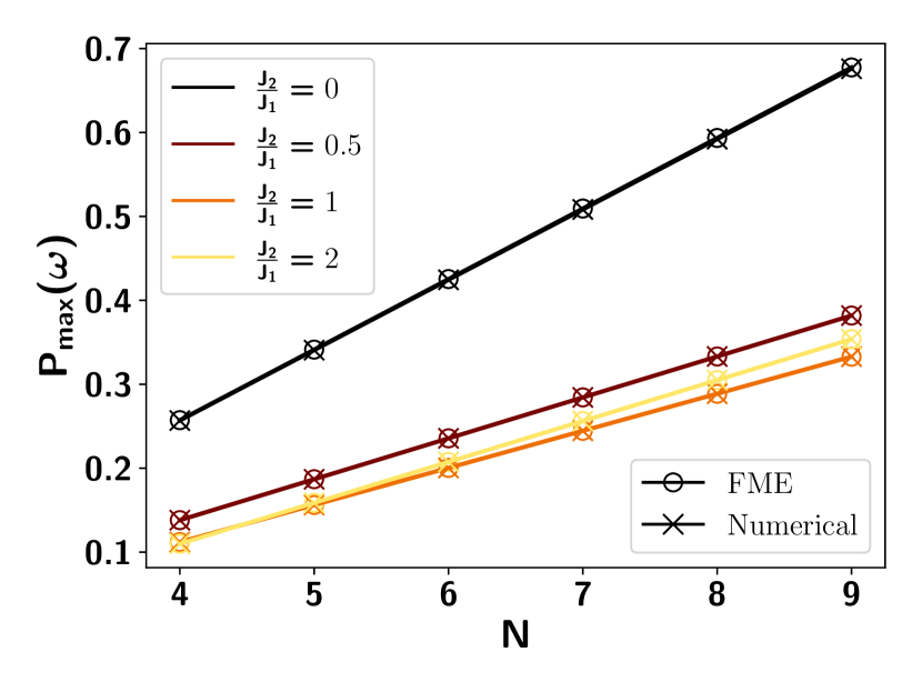
Figure 3: Scaling analysis for charging Hamiltonian with NN and NNN inetractions. $P_{max}(\omega)$ (vertical axis) against $N$ (horizontal axis). Here $\omega=25$ and $h_{z}=0.5$. Dark to light solid lines represent the increase of the values of $\frac{J_{2}}{J_{1}}$. The scaling of $P_{\max}(\omega)$ is computed both by Floquet-Magnus expansion and by numerical methods which match exactly. It is evident from the figure that $P_{max}(\omega)\sim aN+b$ where $(a,b)$ depends on the $\frac{J_{2}}{J_{1}}$ values. For example, for $\frac{J_{2}}{J_{1}}=0,\,(0.084,-0.079)$; $\frac{J_{2}}{J_{1}}=0.5,\,(0.0487,-0.0569)$; $\frac{J_{2}}{J_{1}}=1,\,(0.044,-0.065)$; and $\frac{J_{2}}{J_{1}}=2,\,(0.048,-0.085)$. Both the axes are dimensionless.

To perform the scaling analysis analytically, we will derive the time-independent Floquet Hamiltonian for the charging by using Floquet-Magnus expansion (FME) Magnus (1954); Blanes et al. (2009); Bukov et al. (2015). Since the charging Hamiltonian is periodic in time, i.e., $H_{ch}(t)=H_{ch}(t+T)$, we invoke Floquet theory to study the dynamics of the quantum battery. We calculate the time-independent Floquet Hamiltonian, $H_{ch}^{F}[t_{0}]$, which can be used to evolve the system at stroboscopic time periods $\tau$ ($\tau\ \epsilon\ n(T+t_{0})\ \forall\ n\ \epsilon\,\mathbb{Z}^{+}$) as

$$U^{F}(\tau,t_{0})=e^{(-iH_{ch}^{F}[t_{0}]\tau)}.$$ (7)

We fix $t_{0}=0$, thereby neglecting $[t_{0}]$ further in our calculation. To compute $H_{ch}^{F}$ in the high frequency limit, i.e., when $\omega$ is high enough, we use the Floquet-Magnus expansion upto $O(T^{3})$ terms and rewrite the charging Hamiltonian in Eq. (6) as

$$H^{F}_{ch} =H^{F_{0}}+H^{F_{1}}+H^{F_{2}}+H^{F_{3}},$$ (8)

where

$$H^{F_{0}} = \frac{H_{1}+H_{2}}{2},\,\,H^{F_{1}}=-i\frac{T}{8}[H_{2},H_{1}],$$

$$H^{F_{2}} = -\frac{T^{2}}{96}\big{[}[H_{2},H_{1}],H_{1}-H_{2}\big{]},$$

$$H^{F_{3}} = i\frac{T^{3}}{384}\big{[}H_{2},[[H_{2},H_{1}],H_{1}]\big{]},$$ (9)

with

$$H_{1} =h_{z}\sum_{j}\sigma_{j}^{z}+\frac{J_{1}^{\prime}}{2}\sum_{j}\big{(}\sigma_{j}^{x}\sigma_{j+1}^{x}+\gamma\sigma_{j}^{y}\sigma_{j+1}^{y}\big{)}$$

$$\quad+\frac{J_{2}^{\prime}}{2}\sum_{j}\big{(}\sigma_{j}^{x}\sigma_{j+2}^{x}+\gamma\sigma_{j}^{y}\sigma_{j+2}^{y}\big{)},$$ (10)

$$H_{2} =h_{z}\sum_{j}\sigma_{j}^{z}-\frac{J_{1}^{\prime}}{2}\sum_{j}\big{(}\sigma_{j}^{x}\sigma_{j+1}^{x}+\gamma\sigma_{j}^{y}\sigma_{j+1}^{y}\big{)}$$

$$\quad-\frac{J_{2}^{\prime}}{2}\sum_{j}\big{(}\sigma_{j}^{x}\sigma_{j+2}^{x}+\gamma\sigma_{j}^{y}\sigma_{j+2}^{y}\big{)}.$$ (11)

Using Eqs. (10) and (11) with $J_{i}=J_{i}^{\prime}/2$ ($i=1,2$), we can explicitly write

$$H^{F_{0}} =h_{z}\sum_{j}\sigma_{j}^{z}$$

$$H^{F_{1}} =\frac{T}{2}(1-\gamma)h_{z}\Bigg{[}J_{1}\sum_{j}(\sigma_{j}^{y}\sigma_{j+1}^{x}+\sigma_{j}^{x}\sigma_{j+1}^{y}),$$

$$\quad+J_{2}\sum_{j}(\sigma_{j}^{y}\sigma_{j+2}^{x}+\sigma_{j}^{x}\sigma_{j+2}^{y})\Bigg{]}$$

$$H^{F_{2}} =-\frac{T^{2}}{3}(1-\gamma)h_{z}\Bigg{[}(J_{1}^{2}+J_{2}^{2})(1-\gamma)\sum_{j}\sigma_{j}^{z},$$

$$\quad+J_{1}J_{2}\sum_{j}(\sigma_{j}^{z}\sigma_{j+1}^{x}\sigma_{j+2}^{x}-\gamma\sigma_{j}^{z}\sigma_{j+1}^{y}\sigma_{j+2}^{y})$$

$$\quad+J_{1}J_{2}\sum_{j}(\sigma_{j}^{x}\sigma_{j+1}^{x}\sigma_{j+2}^{z}-\gamma\sigma_{j}^{y}\sigma_{j+1}^{y}\sigma_{j+2}^{z})$$

$$\quad+J_{1}J_{2}\sum_{j}(\sigma_{j}^{x}\sigma_{j+1}^{z}\sigma_{j+3}^{x}-\gamma\sigma_{j}^{y}\sigma_{j+1}^{z}\sigma_{j+3}^{y}),$$

$$\quad+J_{1}J_{2}\sum_{j}(\sigma_{j}^{x}\sigma_{j+2}^{z}\sigma_{j+3}^{x}-\gamma\sigma_{j}^{y}\sigma_{j+2}^{z}\sigma_{j+3}^{y})$$

$$\quad+J_{1}^{2}\sum_{j}(\sigma_{j}^{x}\sigma_{j+1}^{z}\sigma_{j+2}^{x}-\gamma\sigma_{j}^{y}\sigma_{j+1}^{z}\sigma_{j+2}^{y})$$

$$\quad+J_{2}^{2}\sum_{j}(\sigma_{j}^{x}\sigma_{j+2}^{z}\sigma_{j+4}^{x}-\gamma\sigma_{j}^{y}\sigma_{j+2}^{z}\sigma_{j+4}^{y})\Bigg{]},$$

and so on. For FME expansion, we consider $H_{ch}^{F}$ instead of $H_{ch}$ in Eq. (4).

Let us now investigate how $P_{\max}(\omega)$ scales with $N$ obtained analytically using FME and by explicit numerical simulation for a high values of $\omega$. We find that for a fixed $h_{z}$ and a high $\omega$, $P_{\max}(\omega)\sim aN+b$ where $a$ and $b$ are constants. We observe that the scaling with $N$ for different $J_{2}/J_{1}$ values via numerical simulation exactly matches with the one obtained by using FME (see Fig. 3 with $\omega=25$). It demonstrates that despite the presence of next-nearest neighbor term in the charging Hamiltonian, the scaling cannot be made super-extensive which indicates that SR interactions are not enough to attain super-linear scaling in power.

III Super-linear scaling with long-range system Via Floquet driving

We now delve into the charging Hamiltonian involving long-range interactions. It was shown that the maximum power with charging being with NN interactions scales linearly through Floquet driving although Floquet charging involves effectively $N$-body interaction Mondal and Bhattacharjee (2022). We exhibit here that a super-extensive scaling of average power can be achieved if charging is done through the long-range interacting Hamiltonian provided Floquet frequency is tuned appropriately. Interestingly, we also show that such scaling cannot be achieved by unitary evolution.

III.1 Super-extensive scaling of power for LMG model

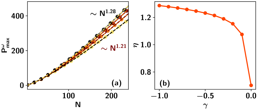
Figure 4: Scaling analysis for LMG charging Hamiltonian. (a) $P_{\max}^{\omega}$ (ordinate) with system-size $N$ (horizontal axis), when the charging Hamiltonian is the two-body LR $XY$ model with $\alpha=0$. By least-square fitting method, we find that it scales as $P_{\max}^{\omega}\sim aN^{\eta}+b$, where $a$ and $b$ are constants, with $\eta>1$ as mentioned in the figure. (b) Dependence of $\eta$ (ordinate) on $\gamma$ (abscissa) which shows the scaling upto $\approx 1.3$. Other parameters are $h_{z}=1$, and $J=20$. All the axes are dimensionless.

In order to show the super-linear scaling, we have to demonstrate that the maximum average power after optimizing over stroboscopic time and the driven frequency, scales as

$$P_{\max}^{\omega}\sim aN^{\eta}+b,$$ (12)

with the scaling exponent,$\eta>1$ and $a$, and $b$ being constants. $\eta=1$ corresponds to the linear scaling as observed with NN interacting charging Hamiltonian and when the evolution is governed by the time-independent unitary operator Julià-Farré et al. (2020); Dou et al. (2022). We will be presenting the scaling analysis in two parts – (1) LR interacting Hamiltonian with $\alpha=0$ and $Z=N-1$ which represents the LMG model Lipkin et al. (1965); (2) persistence of superlinear scaling for $0\leq\alpha\leq 1$, which represents the LR $XY$ model.

Scaling in the LMG model. For $\alpha=0$, the LMG Hamiltonian can be represented in the angular momentum basis, reducing the dimension of the system from $2^{N}\times 2^{N}$ to $N\times N$ which show several exotic properties Dusuel and Vidal (2004); Vidal et al. (2004); Dusuel and Vidal (2005). Specifically, we can rewrite the Hamiltonian as

$$H_{int}^{LR} = \frac{J}{2N}[(1+\gamma)(S_{+}S_{-}+S_{-}S_{+}-N)$$ (13)

$$+(1-\gamma)(S_{+}^{2}+S_{-}^{2})]+S_{z},$$

where $S_{l}=\frac{1}{2}\sum_{i}\sigma_{l}^{z}$ where $l\in\{x,y,z\}$ and $S_{\pm}=S_{x}\pm iS_{y}$. Such a formalism allows us to obtain $P_{\max}^{\omega}$ for a large system-size which is not possible for $\alpha\neq 0$. We observe that when $-1\leq\gamma\leq 0$, the scaling exponent in the maximum average power lies above unity, i.e., $1<\eta\leq 1.5$, as depicted in Figs. 4. Eg. when $h_{z}/J=0.05$ and $\gamma=-1.0$, the scaling equation reads as $P_{\max}^{\omega}=aN^{1.28}+b$ where $a=0.39$, $b=-2.24$ and mean square error is $0.16\%$ (see Fig. 4). It also highlights that $\gamma=-1$ is the best choice to obtain super-linear scaling compared to any values from $\gamma<0$. This can be intuitively understood as the norm of the commutator, i.e, $\|[H_{B},H_{int}^{LR}]\|$, maximizes when $\gamma<0$.

Competitions between magnetic field and interaction strengths in scaling and power. Let us now study how the scaling exponent, $\eta$, depends on the ratio between the strength of the magnetic field and the interaction, $h_{z}/J$. When the interaction strength dominates over the strength of the magnetic field, i.e., when $\frac{h_{z}}{J}\ll 1$ (in the paramagnetic phase), we observe the non-linear scaling with $\eta>1$ while for $\frac{h_{z}}{J}>1$ (in the ferromagnetic phase), the scaling remains extensive although the magnitude of $P_{\max}^{\omega}$ is higher than that for $h_{z}/J>1$. Notice, further, that with the increase of $J$ such that $h_{z}/J\ll 1$, the scaling exponent increases and, finally, it saturates to $N^{1.5}$.

Floquet vs quench driving. In the ferromagnetic phase ($\frac{h_{z}}{J}>1$), the maximum average power via Floquet drive far exceeds the quench-based drives (i.e., $\omega\rightarrow 0$) both with respect to the scaling (although non-super-extensive) and the magnitude of power while in the paramagnetic phase, opposite picture emerges. Specifically, for $\frac{h_{z}}{J}<1$, $P_{\max}^{\omega}$ through the time-independent unitary charging is higher than that of the Floquet drive provided the system-size is moderate. For a large system-size, again Floquet-driven power becomes the best.

III.2 Scaling with power-law fall-off rate

We now investigate how the scaling and other behavior of $P_{\max}^{\omega}$ change with the increase of $\alpha$. Firstly, when $\alpha\leq 2$ along with $\gamma=-1$, the numerical simulation reveals that the charging Hamiltonian in Eq. (1) in the paramagnetic phase ($h_{z}/J\ll 1$) continues to provide super-extensive scaling. In particular, the scaling exponent, $\eta$ in Eq. (12), increases with the decrease of $\alpha$ (as shown in Fig. 5) and achieves its maximum when $\alpha\rightarrow 0$. This result clearly exhibits that the long range interactions (both in LR and quasi LR regimes) along with periodic driving lead to a significant increase in the scaling as opposed to the short range interactions involved in the charging Hamiltonian. This implies that the super-linear scaling is possibly related to the capability possessed by the driving Hamiltonian in terms of distributing entanglement among sites Lakkaraju et al. (2021). Further, we notice that when $\alpha\gg 2$, the scaling even with Floquet driving becomes linear with $N$. Eg. for $\alpha=5$ and $h/J=0.1$, $P_{\max}^{\omega}\sim aN+b$ with $a=0.32,\,\text{and}\,b=0.04$.

Response of coordination number in the scaling of the model. We have already shown that the scaling of $P_{\max}^{\omega}$ is super-extensive when $0\leq\alpha\leq 2$, $\gamma<0$ and $Z=N-1$. Let us now ask the following question – “how does this super-linear scaling and magnitude of power depend on the range of interactions in the long-range domain?” Again, we start our analysis of the charging Hamiltonian by fixing $h_{z}/J\ll 1$. Firstly, the magnitude of $P_{\max}^{\omega}$ increases with $Z$ for different $\alpha\leq 2$ values, belonging to LR and quasi long-range regimes and in the domain where $J\gg h_{z}$. In particular, as $\alpha$ increases, the maximum power does not change significantly with $Z$ while for small $\alpha$, especially when $\alpha<1$, $P_{\max}^{\omega}$ increases monotonically with $Z$ (see Fig. 6). This is possibly due to the fact that strong long-range interaction is capable of creating high entanglement among all the sites, leading to a greater quantum advantage in QB in comparison with the nearest-neighbor or few neighbor interacting charger.

In the context of scaling, we already know two extreme cases: $Z=2$ gives linear scaling, i.e., $\eta=1$ as shown in Sec. II while $Z=N-1$, $\eta=1.5$ with $\alpha\leq 2$. It is evident from Fig. 7 that with the increase of $Z$, the scaling exponent, $\eta$, increases.

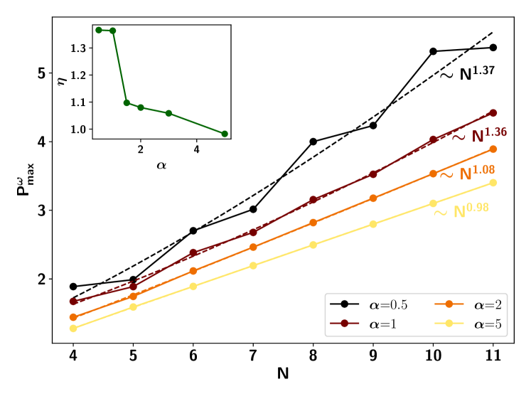
Figure 5: Scaling of LR $XY$ charging Hamiltonian. Behavior of $P_{\max}^{\omega}$ against system-size $N$ with $h_{z}=0.5$, $J=5$, $\gamma=-1$. Periodic driving along with LR interaction induces super-extensive scaling, i.e., when $\alpha<2$, $P_{\max}^{\omega}\sim aN^{\eta}+b$ with $\eta>1$ and $a$, $b$ being constants. Inset depicts how super-linear scaling exponent $\eta$ (vertical axis) changes with LR interaction strength $\alpha$ (horizontal axis). Both the axes are dimensionless.

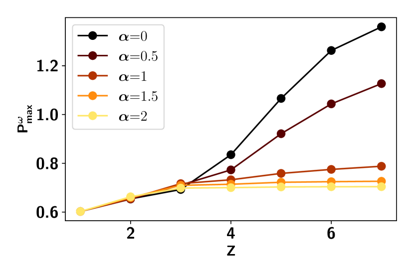
Figure 6: $P_{\max}^{\omega}$ (ordinate) vs coordination number $Z$ (abscissa) with $\gamma=-1$. Dependency upon $Z$ is displayed for different long-range strength, $\alpha$, in the long-range $XY$ model. Other system parameters are $J=20$, $h_{z}=0.5$ and $N=8$. Clearly, low $\alpha$ and high $Z$ provides high $P_{\max}^{\omega}$. Both the axes are dimensionless.

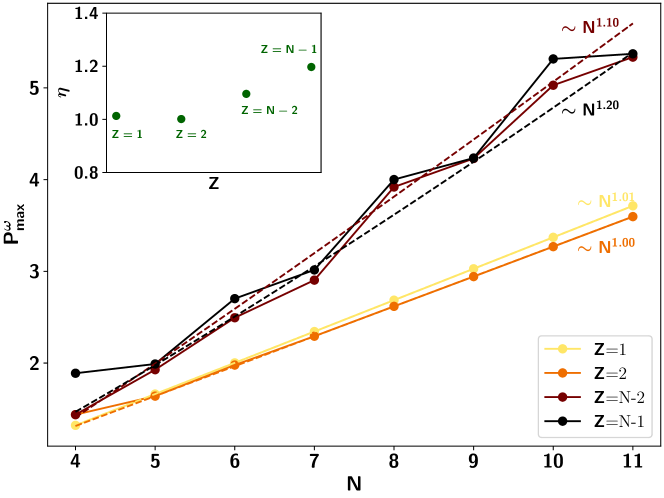
Figure 7: Scaling of $P_{\max}^{\omega}$ (ordinate) vs system-size $N$ (abscissa) with $\gamma=-1$ and $\alpha=0.5$. Dependency upon $N$ is displayed for different coordination number $Z$ in the long-range $XY$ model. Other system parameters are $J=5$, $h_{z}=0.5$ and $N=8$. Inset displays $\eta$ (vertical axis) with respect to $Z$ (horizontal axis). It clearly indicates the influence of $Z$ on achieving super-extensive scaling in $P_{\max}^{\omega}$ as $\eta$ increases with $Z$. All the axes are dimensionless.

IV Scaling with extended $XY$ model

In order to compute the average maximum power with the charging being the extended $XY$ model in Eq. (2), we first rewrite the Hamiltonian in the fermionic basis following the Jordan-Wigner transformation Lieb et al. (1961); Barouch et al. (1970); Barouch and McCoy (1971); Mbeng et al. (2024) as

$$\sigma^{x}_{n} =\left(c_{n}+c_{n}^{\dagger}\right)\prod_{m<n}(1-2c^{\dagger}_{m}c_{m}),$$

$$\sigma^{y}_{n} =i\left(c_{n}-c_{n}^{\dagger}\right)\prod_{m<n}(1-2c^{\dagger}_{m}c_{m}),$$

$$\text{and}\quad\sigma^{z}_{n} =1-2c^{\dagger}_{n}c_{n},$$ (14)

where $c_{m}^{\dagger}$($c_{m}$) is the creation (annihilation) operator of spinless fermions and they follow fermionic commutator algebra. The Hamiltonian in such basis reads as

$$H_{int}^{extXY} = \sum_{n}\sum_{r}\frac{J_{r}(t)}{2}[(1+\gamma)c_{n}^{\dagger}c_{n+r}+(1-\gamma)c_{n}^{\dagger}c_{n+r}^{\dagger}$$ (15)

$$+ \text{h.c}].$$

We prepare the initial state as the ground state of $H_{B}=\frac{h_{z}}{2}\sum_{j}\sigma_{j}^{z}$ and it is evolved through $H_{ch}=H_{B}+H_{int}^{extXY}$ which can be mapped to a quadratic free fermionic model given in Eq. (15). To compute the power of the battery, we rewrite the charging Hamiltonian in the momentum space by performing a Fourier transform of $c_{n}=\frac{1}{\sqrt{N}}\sum e^{-i\phi_{k}}c_{k}$ where $\phi_{k}=\frac{(2k-1)\pi}{N}$ $\forall k\in\pm[1,N/2]$ (we consider periodic boundary condition for this integrable model) and in this space, the model is described as $H_{int}^{extXY}=\underset{k\geq 0}{\bigoplus}\Psi_{k}H_{k}\Psi_{k}^{\dagger}$ where

$$H_{k}=\begin{bmatrix}\text{Re}(J_{k}^{\alpha}(t))(1+\gamma)-h_{z}&i\text{Im}(J_{k}^{\alpha}(t))(1-\gamma)\\ -i\text{Im}(J_{k}^{\alpha}(t))(1-\gamma)&-\text{Re}(J_{k}^{\alpha}(t))(1+\gamma)+h_{z}\end{bmatrix},$$ (16)

with $J_{k}^{\alpha}=\sum_{r=1}^{\frac{N}{2}}J_{r}e^{i\phi_{k}r}$ and $\Psi_{k}^{\dagger}=(c_{k}\quad c_{-k}^{\dagger})$ being the Bogoliubov basis. Hence, the effective unitary that can describe the stroboscopic evolution of QB for each mode $k$ is given as

$$U_{k} = \exp(-iH_{k}(-J)\frac{T}{2})\exp(-iH_{k}(+J)\frac{T}{2})$$ (17)

$$= \exp(-H_{k}^{F}T),$$

where $H_{k}^{F}$ is the Floquet Hamiltonian. This Hamiltonian can be evaluated since $H_{k}^{F}=\sum_{k\geq 0}\beta_{T}(k)\vec{n}_{k}.\vec{\sigma}_{k}$ with $\vec{n}_{k}=\frac{1}{\sqrt{1-u_{k}^{0}}}\begin{bmatrix}u^{x}_{k},&u^{y}_{k},&u^{z}_{k}\end{bmatrix}$ and $\beta_{T}(k)=\frac{1}{T}\cos^{-1}u_{k}^{0}$. Here $\vec{\sigma_{k}}$ are the Pauli matrices in the Bogoliubov basis. The elements of $\vec{n}_{k}$ read as

$$u_{k}^{0} = \cos(\frac{E_{k}^{1}T}{2})\cos(\frac{E_{k}^{2}T}{2})$$

$$-\cos(\Delta_{k})\sin(\frac{E_{k}^{2}T}{2})\sin(\frac{E_{k}^{1}T}{2}),$$

$$u^{x}_{k} = \sin(\frac{E_{k}^{1}T}{2})\sin(\frac{E_{k}^{2}T}{2})\sin(\Delta_{k}),$$

$$u^{y}_{k} = \cos(\frac{E_{k}^{1}T}{2})\sin(\frac{E_{k}^{2}T}{2})\sin(\theta_{k}^{2})$$

$$+\cos(\frac{E_{k}^{2}T}{2})\sin(\frac{E_{k}^{1}T}{2})\sin(\theta_{k}^{1}),$$

$$u^{z}_{k} = -\cos(\frac{E_{k}^{1}T}{2})\sin(\frac{E_{k}^{2}T}{2})\cos(\theta_{k}^{2})$$ (18)

$$-\cos(\frac{E_{k}^{2}T}{2})\sin(\frac{E_{k}^{1}T}{2})\cos(\theta_{k}^{1}),$$

where $E_{k}^{i}=\sqrt{(\text{Re}(J_{k}^{\alpha})_{i}-h_{z})^{2}+\text{Im}(J_{k}^{\alpha})_{i}^{2}}$, $\cos(\theta_{k}^{i})=(\text{Re}(J_{k}^{\alpha})_{i}-h_{z})/E_{k}^{i}$ with $i\in\{1,2\}$ and $\Delta_{k}=\theta_{k}^{1}-\theta_{k}^{2}$.

Therefore, the energy stored in the QB at the $n^{th}$ stroboscopic time can be analytically obtained as $W(nT)=\sum_{k\geq 0}\bra{0_{k}}(U_{k}^{\dagger})^{n}H_{B,k}(U_{k})^{n}\ket{0_{k}}-\bra{0_{k}}H_{B,k}\ket{0_{k}}$ with $\ket{0_{k}}$ is the initial state and $H_{B,k}=-h_{z}\sigma^{z}_{k}$ is the battery Hamiltonian in the momentum space. The work output takes the form as

$$W(nT)=\sum_{k\geq 0}2h_{z}(1-(n_{z}^{k})^{2})\sin^{2}(n\cos^{-1}u_{k}^{0}).$$ (19)

It is evident from the above expression that the work in the stroboscopic time depends nonlinearly on the frequency of the Floquet driving, $T=2\pi/\omega$. Clearly, it is a function of $\omega$, $\alpha$, $h_{z}$ and $J$, i.e., $f(\alpha,\omega,h_{z},J)$ which indicates that by calibrating $\omega$, $\alpha$ and $h_{z}/J$, we can obtain nonlinear scaling in the maximum average power, $P_{\max}^{\omega}$ with system-size as presented in Fig. 8. The figure illustrates that $P_{\max}^{\omega}\sim aN^{\eta}+b$, with $\eta>1$ when we are in deep long-range regime with $0\leq\alpha<1$. It again establishes the genuine quantum advantage of long-range interactions during charging of the QB through Floquet driving. However, super-extensive scaling, in this case, cannot be accomplished in the quasi long-range domain ($1<\alpha<2$) which is, in contrast, to the LR $XY$ model presented in Sec. III.

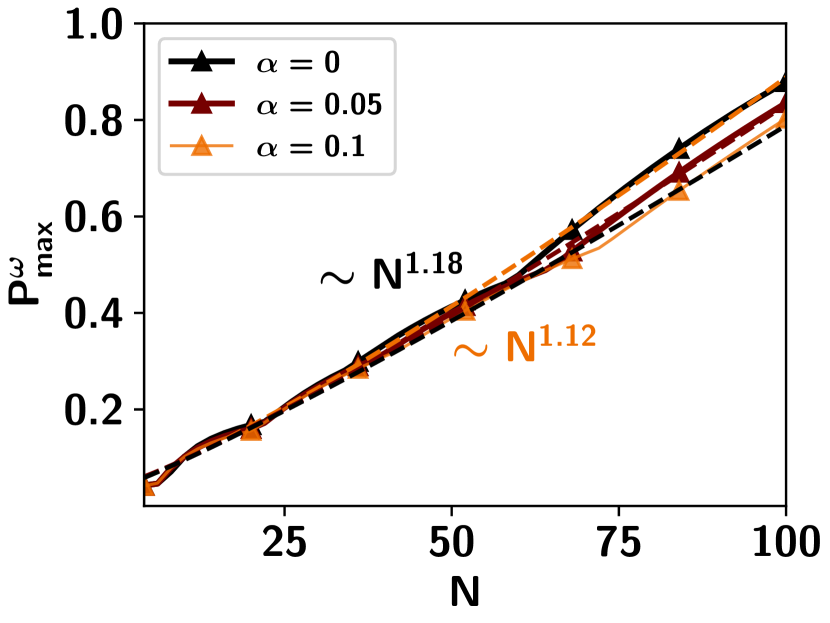
Figure 8: Scaling analysis for LR extended $XY$ charging Hamiltonian. $P_{\max}^{\omega}$ (ordinate) with system-size $N$ (horizontal axis) for different fall-off rates $\alpha$. Other parameters are $h_{z}=0.02$, $J=1$ and $\gamma=-1$. Again, by least square fitting, we find $P_{\max}^{\omega}\sim aN^{\eta}+b$ where $a$ and $b$ are constants and $\eta>1$ as mentioned in the figure for low $\alpha$ values and $Z=N-1$. Both the axes are dimensionless.

V Conclusion

Floquet engineering has become a useful tool to showcase several exotic phenomenon in physical systems. With the development of various experimental techniques, periodic driving has been recognized as a key strategy for developing quantum technology. Moreover, the application of periodic driving to quantum systems is particularly exciting due to the growing arsenal of experimental techniques, such as ultracold atoms, trapped ions, and superconducting circuits, which allow for the precise implementation of Floquet protocols. Among the various emerging quantum technologies, quantum transistors and quantum batteries (QB) stand out as two prominent areas where Floquet engineering can show significant promise.

In this study, we explored the role of Floquet evolution in enhancing the charging process of quantum batteries (QB), focusing on the maximum average power. We demonstrated that by appropriately tuning the Floquet frequency, quantum advantage can be achieved when the charging is governed by a long-range interaction Hamiltonian. Specifically, our results demonstrate that no quantum advantage exists when the system is charged using a next-nearest neighbor interacting model, even when the Floquet frequency is optimized. In contrast, when charging is governed by a long-range interacting model, a clear quantum advantage emerges in the deep long-range regime. In this regime, the power scales super-linearly with system-size. In particular, the scaling behavior depends on both the parameters of the charging Hamiltonian and the strength of the long-range interactions, characterized by the fall-off rate. We find that as the fall-off rate increases, the scaling decreases, suggesting that weaker long-range interactions diminish the quantum advantage.

Our analysis shows that the impact of fall-off rate and the range of interactions in the scaling analysis of power is not at all straightforward. Specifically, the effect of increasing long-range interactions on the charging can be either beneficial or detrimental, depending on the specific region of the parameters under consideration. This non-monotonic behavior reflects the intricate interplay between the interaction strength, the Floquet frequency, and the underlying Hamiltonian structure.

In summary, our findings indicate that a genuine quantum advantage in the charging of quantum battery can be realized in the context of periodic driving through long-range interactions. The results also reveal the potential of periodic driving and long-range interactions as crucial tools in the development of effective quantum energy storage systems and quantum technologies, in general, emphasizing the delicate balance that must be found between system parameters to attain maximum performance.