Distinguish the environmental effects and modified theory of gravity with multiple massive black-hole binaries

Abstract

In the typical data analysis and waveform modelling of the gravitational waves signals for binary black holes, it’s assumed to be isolate sources in the vacuum within the theory of general relativity (GR). However, various kinds of matters may exist around the source or on the path to the detector, and there also exist many different kinds of modified theories of gravity. The effects of these modifications can be characterized within the parameterized post-Einstein (ppE) framework, and the corresponding phase corrections on the waveform at leading post-Newtonian (PN) order are also expressed by the additional parameters for these effects. In this work, we consider the varying-G theory and the dynamical friction of the dark matter spike as an example. Both of these two effects will modify the waveform at -4PN order, if we choose the suitable power law index for the spike. We choose to use a statistic to characterize the dispersion between the posterior of $\dot{G}$ for different events. For different astronomical models, we find that this statistic can distinguish these two models very effectively. This result indicates that we could use this statistic to distinguish other degenerate effects with the detection of multiple sources.

I Introduction

In the 2030s there expected to have multiple space-borne GW detectors on operation, including TianQin Luo et al. (2016); Mei et al. (2021), LISA Danzmann (1997); Amaro-Seoane et al. (2017), and TaijiHu and Wu (2017). These detectors will focus on the millihertz frequency band of GW, and observe many different kinds of sources, such as Galactic Compact Binaries Korol et al. (2017); Huang et al. (2020), massive black hole binarys Klein et al. (2016); Wang et al. (2019); Feng et al. (2019), the inspiral of Stellar Mass Black Hole Binaries Sesana (2016); Kyutoku and Seto (2016); Liu et al. (2020), extreme mass-ratio inspirals Babak et al. (2017); Fan et al. (2020), and Stochastic GW Background Caprini et al. (2016); Bartolo et al. (2016); Liang et al. (2022); Cheng et al. (2022). Due to the longer duration and larger signal-to-noise ratio (SNR) of the signals, the parameter estimation (PE) accuracy will also be much higher. Thus it will have significant improvements on the study of fundamental physics Gair et al. (2013); Barausse et al. (2020); Arun et al. (2022), astrophysics Seoane et al. (2023); Baker et al. (2019) and cosmology Tamanini et al. (2016); Zhu et al. (2022a); Auclair et al. (2023); Caldwell et al. (2019); Zhu et al. (2022a, b). One of the most important topics is to study the nature of gravity and black holes in the strong field regime Shi et al. (2019, 2023); Zi et al. (2021); Xie et al. (2022); Kong and Zhang (2024); Tan et al. (2024); Rahman et al. (2023).

However, most of these analysis have assumed ideal situations. According to the analysis in Gupta et al. (2024); Dhani et al. (2024); Lau et al. (2024); Garg et al. (2024); Chandramouli et al. (2024) , many different effects may cause false GR violation in the observation of GR. These effects can be classified into noise systematics, waveform systematics, and astrophysical aspects. Then it will be very important to deduce the systematics and distinguish the origin of the possible deviation.

In this work, we will consider the possibility of environmental effects. Although most of the analysis assumed the GW generated by isolated sources propagating in the vacuum, there could exist matter surrounding the source or laying on the path. For the matter laying on the path, gravitational lensing will happenLin et al. (2023); Tambalo et al. (2023); Çalışkan et al. (2023). For the matter surrounding the source, there could be dark matter halo and accretion disk. For the binaries immersed in these environments, they will experience accretion, gravitational pull and dynamical frictionBarausse et al. (2014). In this work, we will focus on the dark matter spikeGondolo and Silk (1999a) around the MBHBs in the center of the galaxies. It’s pointed out inBarausse et al. (2014) that the dynamical friction will dominate the evolution of the binaries, and thus it should be the leading order effect. The waveform corrections of dark matter mini-spikes, through gravitational pull and dynamical friction force respectively are investigated in Eda et al. (2013, 2015a). The eccentricity is also taken into account in Gen-Liang Li (2022). With the observed events of LIGO, the density is constrained in Caneva Santoro et al. (2023). After introducing the dark matter (DM) spike,Wilcox et al. (2024) find that the systematic errors can be significantly reduced below the statistic errors if $\gamma=\frac{7}{3}$.

Although the best source to constrain the environment effects is the binaries with large mass ratiosZhao et al. (2024), we will focus on MBHBs with higher certainties in this work. The phase correction due to the environment effect can be expressed in the ppE formalism Yunes and Pretorius (2009); Tahura and Yagi (2018), which is a parameterized framework to describe the deviation from GR on GWs. For both the dynamical friction of dark matter spike with power index $\gamma=\frac{3}{2}$ and the varying-G theory, the phase correction are all introduce at $-4$ PN order. Thus the existence of dark matter may cause false positive result on the varying of gravitational constant.

However, the varying rate of the gravitational constant should be a constant for all the sources, while the property of the dark matter surrounding each sources could be different. With a single event, it will be difficult to distinguish these two effects. But with multiple events, if the deviation is caused by the varying of $G$, we will get a consistent result on the posteriors of $\dot{G}$. On the other hand, if the deviation is cause by dynamical friction (DF) and we misinterpret it as the varying-G theory, we will get a disperse result on the posteriors. Thus by analyzing the dispersion of the posteriors, we can distinguish these two effects.

This paper is organized as follows. In Section II, we give a brief review on the waveform and its correction within the ppE framework, then we focuse on the DF of DM spike for environment effect, and the varying $G$ theory for modified gravity. Then, in Section III, we introduce the fisher information matrix (FIM) used for PE, and analysed the accuracy on the measurement of $\rho_{0}$ for both varying the source parameters and using the astronomical models. In Section IV, we give the correspondence between $\rho_{0}$ and $\dot{G}$, and introduce the statistic to characterise the dispersion of the posterior for the events observed. Then we calculate the distribution of the statistic distribution for three different models, and analyzed the distinguishability between different models. We give a brief summary and discussion in Section V. Throughout this work, the geometrized unit system ($G=c=1$) is used.

II Waveform Model

There exist many different kinds of models for the modified theory of gravity and the environment surrounding the binaries. However, all the effects on the waveform can be characterised within the ppE framework. In this section, we first introduce the ppE formalism with higher mode phase corrections. Then for a specific model, we introduce the waveform correction due to the dynamical friction of the dark matter spike. We also introduce the waveform correction of the varying-G theory, which will be degenerate with dynamical friction if we choose $\gamma=\frac{3}{2}$

II.1 the ppE framework

In order to describe the leading order corrections on the waveform in a parametric form, the ppE formalism was introduced . When the masses of the components are highly asymmetric, higher modes of gravitational waves will be important in the waveform. According to Mezzasoma and Yunes (2022), the ppE formalism for waveforms with higher modes is

$$\tilde{h}(f)=\sum_{lm}\tilde{h}_{lm}(f)=\sum\tilde{h}^{\text{GR}}_{lm}(f)e^{i\delta\Psi_{lm}}.$$ (1)

In this work, we use IMRPhenomXHM to obtain the GR waveform with higher modes. Since the amplitude correction is nearly negligible, in this work, we will only consider the phase correction which is,

$$\delta\Psi_{lm}=\beta_{lm}u^{b_{lm}}.$$ (2)

$u=(\pi\mathcal{M}_{c}f)^{1/3}$ represents the relative velocity of the binary components, and $\mathcal{M}_{c}=(m_{1}m_{2})^{3/5}/(m_{1}+m_{2})^{1/5}$ is the chirp mass for the binary with component masses $m_{1}$ and $m_{2}$. We will also use the total mass $M=m_{1}+m_{2}$ and the symmetric mass-ratio $\eta=m_{1}m_{2}/(m_{1}+m_{2})^{2}$ in the following parts. The corrections for different higher modes can be represented by that of $22$ mode as

$$\beta_{lm}=\left(\frac{2}{m}\right)^{\frac{b_{lm}}{3}-1}\beta_{22},~~~b_{lm}=b_{22}.$$ (3)

and $m_{1},m_{2}$ are the masses of the components of the binary, and the total mass is $m_{1}+m_{2}=M$. In the following part, we will use $\delta\Psi$ to represent $\delta\Psi_{22}$ for simplicity.

II.2 Dynamical Friction of Dark Matter Spike

If the dark matter is composed by massive particles, then due to the coevolution of the central BH and the dark matter halo, the adiabatic growth of the BH will give rise to a spike citeastro-ph/9906391. Then the density of the dark matter in the spike is much higher than the average density of dark matter in the surrounding halo. The density profile of the spike often have a steeper slope and follows a power law relationship close to the central object.

$$\rho(r)=\rho_{0}\left(\frac{r_{0}}{r}\right)^{\gamma}$$ (4)

where $r$ is the distance to the center of mass of the binary. We have neglect the inner radial cutoff of the spike, since it will be smaller than the radius of the innermost stable circular orbit (ISCO) for the binary. Then the total mass enclosed in the sphere with radius $r$ is

$$m(r)=\frac{4\pi\rho_{0}r_{0}^{\gamma}}{3-\gamma}r^{3-\gamma}$$ (5)

Beside the characteristic radius $r_{0}$, where the density equals to $\rho_{0}$, we can also define $r_{200}$ as the radius where the density is $200$ times of the critical density of the matter $\rho_{cm}$, which is determined by the critical density of our universe $\rho_{c}=9.73\times 10^{-27}\text{kg}/\text{m}^{3}$ Spergel et al. (2003) and the redshift $z$. Thus we will have

$$\rho(r_{200})=\rho_{0}\left(\frac{r_{0}}{r_{200}}\right)^{\gamma}=200\rho_{cm}$$ (6)

If $M$ is the total mass of the central bianry BH, we can determine the parameters of the spike b y assuming that

$$m(5r_{0}) = {4\pi\rho_{0}r_{0}^{\gamma}\over 3-\gamma}(5r_{0})^{3-\gamma}=2M$$ (7)

$$m(r_{200}) = \frac{4\pi\rho_{0}r_{0}^{\gamma}}{3-\gamma}r_{200}^{3-\gamma}=NM.$$ (8)

By solving these equations, we will have

$$\rho_{0} = 200\rho_{cm}5^{\gamma}\left(\frac{N}{2}\right)^{\frac{\gamma}{3-\gamma}}$$ (9)

$$r_{0} = \left(\frac{M(3-\gamma)}{2\pi\rho_{0}}\right)^{\frac{1}{3}}5^{\frac{\gamma-3}{3}}.$$ (10)

In previous studies Eda et al. (2013); Coogan et al. (2022); Binney and Tremaine (2008); Sesana et al. (2014a) $N$ is assumed to be in the range of $10^{3}-10^{6}$. In this study, we will fix $N$ to be $10^{6}$, then if we choose a special value of $\gamma$, both $\rho_{0}$ and $r_{0}$ is determined according to the above formulas.

For the binary immersed in the spike, due to the varying complexion of the near dark matter, the fluctuating force acting on each BH will form the dynamical friction. Thus the BHs will have a systematic tendency to be decelerated in the direction of its motion. For an object with mass $m$ moving in the spike with the orbital radius $r$ with velocity $v$, the magnitude of the dynamical friction is

$$F_{DF}=\frac{4\pi\rho(r)m^{2}I}{v^{2}}$$ (11)

$I$ is a order 1 factor depending on the velocities of components with respect to the mediumKim and Kim (2007). Following the analysis in Eda et al. (2015b), we use $I\cong 3$ in this work.

Therefore, beside the energy loss due to the gravitational radiation, the binaries will also loss energy due to the dynamic friction. Thus the equation for the conservation of energy is

$$-\frac{dE}{dt}=\frac{dE_{GW}}{dt}+\frac{dE_{DF}}{dt}$$ (12)

and we also have

$$\frac{dE_{DF}}{dt}=\sum_{i}F_{DF,i}v^{i}=\sum_{i}\frac{4\pi I\rho(r_{i})m_{i}^{2}}{v_{i}}$$ (13)

Here the index $i=1,2$ denotes the two BHs of the binary. Then following the procedure in Wang et al. (2022), we can find that the phase correction is

$$\delta\Psi_{\text{DF}}=-\frac{75I\pi\rho_{0}r_{0}^{\gamma}}{256(\gamma-8)(2\gamma-19)}Ku^{\frac{2\gamma-11}{3}},$$ (14)

and the factor $K$ is

$$K = (m_{1}^{2}m_{2}^{-\gamma-1}+m_{2}^{2}m_{1}^{-\gamma-1})\mathcal{M}_{c}\eta^{-\frac{2\gamma+2}{5}}$$ (15)

$$= \frac{\left(1+\sqrt{1-4\eta}\right)^{3+\gamma}+\left(1-\sqrt{1-4\eta}\right)^{3+\gamma}}{\mathcal{M}_{c}^{\gamma-2}\eta^{\frac{4\gamma}{5}+2}2^{\gamma+3}}$$

In the following analysis, we will consider $\rho_{0}$ as a parameter that need to be measured, and $\gamma$ is fixed. So $r_{0}$ is determined by $M$ and $\rho_{0}$ according to Eq. (10), and the factor $\rho_{0}r_{0}^{\gamma}$ can be reduced to

$$\rho_{0}r_{0}^{\gamma}=(2\pi)^{-\frac{\gamma}{3}}5^{\frac{\gamma(\gamma-3)}{3}}(3-\gamma)^{\frac{\gamma}{3}}\mathcal{M}_{c}^{\frac{\gamma}{3}}\eta^{-\frac{\gamma}{5}}\rho_{0}^{1-\frac{\gamma}{3}}$$ (16)

When $\gamma=\frac{3}{2}$, we will have

$$\delta\Psi_{\text{DF}}=-\frac{15\sqrt[4]{5}}{851968}\sqrt{\frac{3\pi\rho_{0}}{2}}I\mathcal{M}_{c}\eta^{-\frac{29}{10}}H(\eta)u^{-13}$$ (17)

and $H(\eta)$ is defined to be

$$H(\eta)=\left(\frac{1}{2}+\frac{\sqrt{1-4\eta}}{2}\right)^{\frac{9}{2}}+\left(\frac{1}{2}-\frac{\sqrt{1-4\eta}}{2}\right)^{\frac{9}{2}}$$ (18)

this means that $b=-13$ in this case, and the leading order correction is $-4$ PN.

II.3 The theory of varying G

In GR, gravitational coupling strength $G$ is a constant independent of spacetime. While in the varying $G$ theory, it will change over time Yunes et al. (2010). The rate of changing $\dot{G}$ causes a phase correction Tahura and Yagi (2018) as

$$\delta\Psi_{\dot{G}}=-\frac{25\mathcal{S}}{851968}\dot{G}\mathcal{M}_{c}(\pi\mathcal{M}_{c}f)^{-{13\over 3}}.$$ (19)

According to the analysis in Yunes et al. (2010); Wilcox et al. (2024), for general binaries, the factor $\mathcal{S}$ is

$$\mathcal{S}=11-\frac{35}{2}(s_{1}+s_{2})+\frac{41}{2}\sqrt{1-4\eta}(s_{1}-s_{2}),$$ (20)

and $s_{1,2}$ are the sensitivities for the components. However, for BHs, we will have $s_{1}=s_{2}=\frac{1}{2}$, and thus we will have $\mathcal{S}=-\frac{13}{2}$ Wang et al. (2022).

We can find that the leading order correction of varying-G theory is -4 PN, the same order for which the DF with $\gamma=\frac{3}{2}$. Thus these two effects will have degeneracy, and if we find the -4 PN deviation in the future observations, it will be difficult to identify the origion of this deviation.

III Probe the density of dark matter

In this section, we will analyze the capability to probe the density of the dark matter. Since the

III.1 fisher information matrix

In this section we estimate how space based gravitational wave detector can constraints the sources parameters. The sky-averaged noise power spectral density (PSD) for TianQin is

$$S_{n}(f) = \frac{10}{3}\frac{1}{L^{2}}\left[1+\left(\frac{2fL_{0}}{0.41c}\right)^{2}\right]$$ (21)

$$\times \left[\frac{4S_{a}}{(2\pi f)^{4}}\left(1+\frac{10^{-4}\text{Hz}}{f}\right)+S_{x}\right]$$

where $L=\sqrt{3}\times 10^{5}\text{km}$ is the armlength of TianQin, $\sqrt{S_{a}}=10^{-15}\text{m}\dot{\text{s}}^{-2}\text{Hz}^{-1/2}$ and $\sqrt{S_{x}}=10^{-12}\text{m}\dot{\text{Hz}}^{-1/2}$ are the acceleration and position noise of TianQin, respectively.

For signals with large SNR, the posterior distribution of the relevant parameters can be approximated by a Gaussian distribution around the true value. The corresponding covariance matrix is given by the inverse of Fisher matrix: $\Sigma_{ij}=(\Gamma^{-1})_{ij}$, with

$$\Gamma_{ij}=2\int_{f_{\text{min}}}^{f_{\text{max}}}\frac{\partial_{i}h(f)\partial_{j}h^{\ast}(f)+\partial_{i}h^{\ast}(f)\partial_{j}h(f)}{S_{n}(f)}df$$ (22)

where the partial derivative $\partial_{i}$ corresponding to the $i$-th parameter of $\hat{\theta}=(\mathcal{M}_{c},\eta,\chi_{1},\chi_{2},\rho_{0},D_{L})$ The polarization and inclination angle were not take into account since we have also averaged the orientation of the MBHBs. We considered the “3 month on + 3 month off” observation scheme in our calculation, and assume all the events merged during the observation period. Since the ppE correction is used for the inspiral stage, we will only use the inspiral signal to do the analysis, and thus we will have

$$f_{\text{max}}=f_{\text{ISCO}}=\frac{1}{6\sqrt{6}\pi M}$$ (23)

and

$$f_{\text{min}}=\left(\frac{5}{256}\right)^{3/8}\frac{1}{\pi}\mathcal{M}_{c}^{-5/8}T^{-3/8}$$ (24)

III.2 capability to probe the density

For the parameter of the source, we choose $D_{L}=1\text{Gpc},\chi_{1}=0.9,\chi_{2}=0.8,T=5\text{yr},\phi_{c}={\pi\over 4},\psi=0,\iota={\pi\over 4}$. $\mathcal{M}_{c}$ varies between $10^{4}\sim 10^{7}M_{\odot}$, and $\eta$ varies between $0\sim 0.25$

For the dark matter spike, a typical value for the power index is $\gamma={7\over 3}$ according to the study of Gondolo and Silk (1999b). Thus if we choose $N=10^{6}$, we will have $\rho_{0}=2.79\times 10^{-3}\text{kg}/\text{m}^{3}$. We will also have the $\rho_{0}=8.84\times 10^{-14}\text{kg}/\text{m}^{3}$ for $N=10^{3}$. The PE accuracy for $\rho_{0}$ for MBHBs with different $\mathcal{M}_{c}$ and $\eta$ is plotted in Fig. 1.

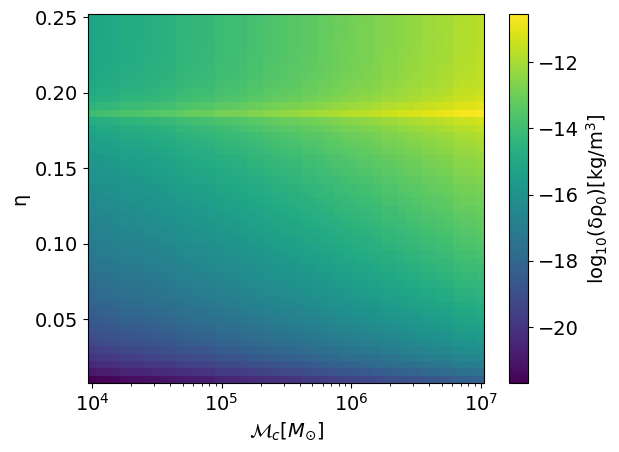
Figure 1: $\gamma={7\over 3}$, adopting $N=10^{6}$ or $\rho_{0}=2.79581\times 10^{-3}\text{kg}\>\text{m}^{-3}$, the $\eta,\mathcal{M}_{c}$ graph of the detection error of $\rho_{0}$.

Since we are trying to distinguish the dark matter spike with the varying-G theory, we also considered the case for $\gamma={3\over 2}$ in Fig. 2 where We adopt $N=10^{6}$ and $\rho_{0}=4.14\times 10^{-18}\text{kg}/\text{m}^{3}$. $\delta\rho_{0}$ for MBHBs with different $\mathcal{M}_{c}$ and $\eta$ is plotted in Fig. 2.

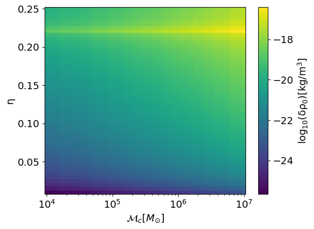
Figure 2: $\gamma={3\over 2}$, the $\eta,\mathcal{M}_{c}$ graph of the detection error of $\rho_{0}$.

We can find that the precession on the measurement of $\rho_{0}$ reach to the level of $10^{-20}\text{kg}/\text{m}^{3}$ or even better for most of the cases. The result will be better for smaller $\eta$ and smaller $\mathcal{M}_{c}$.

Since we will use all the events in the observation to verify if there exist violation of GR, we need to consider astronomical models to simulate the observation data. We consider three different models Barausse (2012); Sesana et al. (2014b); Antonini et al. (2015); Klein et al. (2016)in our work, two heavy-seed models “Q3 d” and “Q3 nod”, and a light-seed model “popIII”. Each model has 1000 mock catalogues for a five year observation with TianQinWang et al. (2019), and the total events number are 18112, 271444, and 56618, respectively. We only consider the events that beyond the SNR threshold. According to these catalogues, we can get $(z,m_{1},m_{2},\chi_{1},\chi_{2},\iota)$ of the sources, then we can calculate $\delta\rho_{0}$ for each source. We use $\gamma=\frac{3}{2}$ in this calculation, and the results are shown in Fig. 3, Fig. 4, and Fig. 5. We labeled each events with the $\mathcal{M}_{c}$ and $\eta$, and the PE accuracy is shown with different colors. We also plot the distribution of $\delta\rho_{0}$ in Fig. 6. The popIII model is shown to have a better precession on probing the density of the spike, and this is due to the fact that the events in this model may have smaller $\eta$.

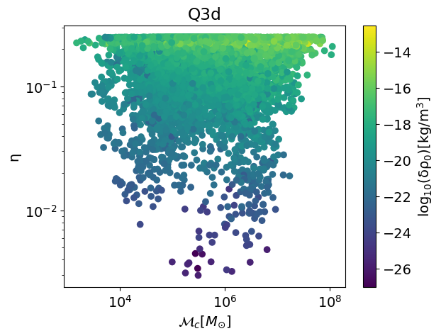
Figure 3: The $\eta,\mathcal{M}_{c}$ graph of the detection error of $\rho_{0}$ of Q3d sources.

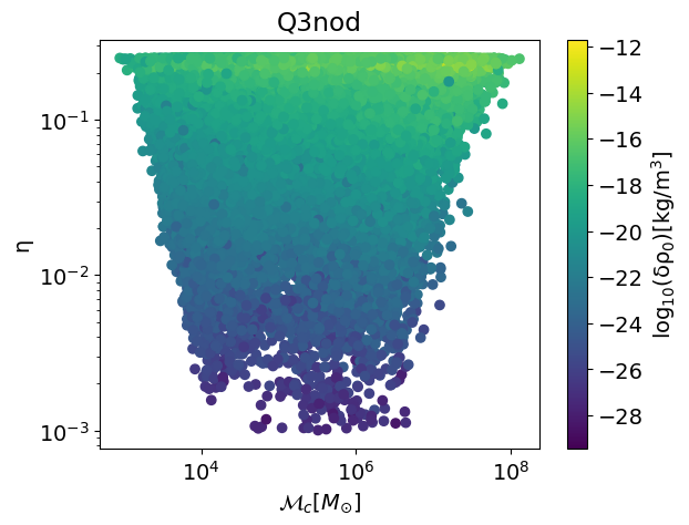
Figure 4: The $\eta,\mathcal{M}_{c}$ graph of the detection error of $\rho_{0}$ of Q3nod sources.

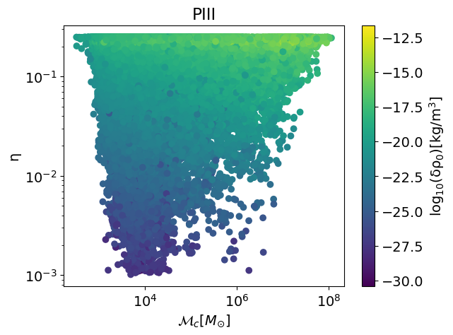
Figure 5: The $\eta,\mathcal{M}_{c}$ graph of the detection error of $\rho_{0}$ of PIII sources.

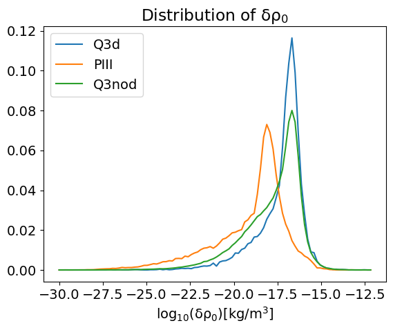
Figure 6: Distributions of $\delta\rho_{0}$ considering Q3d, PIII and Q3nod.

IV Distinguishing dark matter DF and $\dot{G}$ effect

Since both the dynamical friction for the dark matter spike with $\gamma=\frac{3}{2}$, and the varying-G theory will modify the waveform at $-4$ PN order, if we find the deviation at this order in future detections, it will be a very important question to verify which theory is correct. If we neglect the environment effect, we may get false positive results in testing GR. It will be difficult to distinguish these two effects through data analysis of a single event. However, if the detected deviation is caused by varying-G, then the corresponding $\dot{G}$ will be the same for all the events. But if it’s caused by DF, the corresponding $\dot{G}$ will be different for each events. In this section, we will use the results of PE for all the events in the observation period to distinguish these two effects.

IV.1 The relation between DF and $\dot{G}$ theory

If we set the phase correction of DF equal to that of varying-G, we can get that

$$\dot{G}=-\frac{3\sqrt[4]{5}}{65}\sqrt{6\pi\rho_{0}}I\eta^{-\frac{29}{10}}H(\eta)$$ (25)

According to Eq. (9), $\rho_{0}$ only dependent on $\rho_{cm}$, $\gamma$, and $N$, which are all fixed value in our calculation. Then it should be a constant for all the events in our analysis. However, since $\eta$ will be different for each events, the corresponding $\dot{G}$ will also be different.

Then for a MBHBs in a dark matter spike with $\gamma=\frac{3}{2}$, we can pretend it’s caused by the varying of gravitational constant. Then using the value of $\dot{G}$ obtained with Eq. (25), we can get the PE accuracy of each event.

IV.2 The statistic $F$ to distinguish DF and $\dot{G}$

If the modification is caused by varying-G theory, then we should obtain the same value of $\dot{G}$ for all the events. But if the modification is caused by the dynamical friction, according to Eq. (25), the corresponding $\dot{G}$ for each event will be different. So by checking if all the events have a consistent prediction of $\dot{G}$, we can distinguish these two effects. Thus we can use a statistic to to describe the consistency of the values of $\dot{G}$ given by all the events.

We can assume that we have detected $n$ events in our observation, and we find deviations at $-4$ PN order. If we make the hypothesis that the deviation is cause by $\cot G$, then for the $i$-th event, the true value of $\dot{G}$ is $\dot{G}_{i}$, and the corresponding PE accuracy is $\delta\dot{G}_{i}$. So the posterior of $\dot{G}$ for the $i$-th event can be approximated as a normal distribution: $\dot{G}\sim N\left(\dot{G}_{i},\delta\dot{G}_{i}\right)$. Due to the existence of the instrument noise, the center of this distribution $\dot{G}_{i}^{p}rime$ will deviate the true value, and it should also obey this distribution $\dot{G}_{i}^{\prime}\sim N\left(\dot{G}_{i},\delta\dot{G}_{i}\right)$.

Then for all the events, we can define the mean value of the central value of each event as

$$\overline{\dot{G}^{\prime}}=\frac{1}{n}\sum_{i=1}^{n}\dot{G}_{i}^{\prime}.$$ (26)

Then we can define a statistic $F$ to characteristic the dispersion of the posteriors of all the events.

$$F=\frac{\sum_{i=1}^{n}\left(\dot{G}^{\prime}_{i}-\overline{\dot{G}^{\prime}}\right)^{2}}{\sum_{i=1}^{n}\delta G_{i}^{2}}$$ (27)

If all the events have the same central value, we will have $F=0$. However, due to the random error in the PE, it will be a small number instead of the exactly zero. On the other hand, if the central values are totally different, and the PE accuracy is much smaller than the differences, we will get a very large $F$.

For dynamical friction, $\dot{G}_{i}$ is obtained with Eq. (25). The distribution of $\dot{G}_{i}$ for each model is shown in Fig. 7. For the case of varying-G theory, $\dot{G}_{i}$ is a constant. In our analysis, we consider three situations, corresponding to $\dot{G}=0,10^{-14},10^{-7}\text{yr}^{-}1$ respectively. Here $0$ corresponding to GR, and $10^{-14}$ is about the current constraint of $\dot{G}$, while $10^{-7}$ is the typical value caused by dynamical friction as shown in Fig. 7.

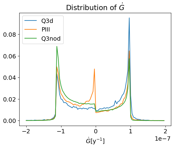
Figure 7: Distributions of $\dot{G}$ considering Q3d, PIII and Q3nod.

For each catalog of a specific astronomical model, we can calculate the statistic $F$ as the procedure we described above. Then we can get the distribution of $F$ with all the 100 catalogs for each cases. The results are shown in Fig. 8, Fig. 9, and Fig. 10 respectively. We can see that for all three models, the distribution of the statistic is totally different for varying-G theory and dynamical friction. No matter what’s the true value of $\dot{G}$, all the three choices will give similar distributions of $F$, since the PE accuracy $\delta\dot{G}$ is not sensitive to the value of $\dot{G}$. For dynamical friction, $F$ will be about $10^{6}\sim 10^{8}$, and it will be smaller than $10$ for varying-G theory. Thus in the real detection, if we get a $F$ much larger than $10$, we can say it’s cause by the environmental effect definitely.

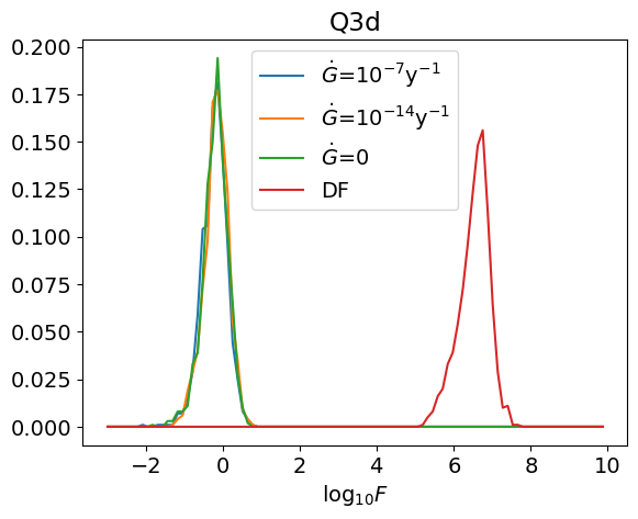
Figure 8: The distribution of $F$ for Q3 d model for different values of $\dot{G}$ in varying-G theory and the dynamical friction of dark matter spike with $\gamma=\frac{3}{2}$.

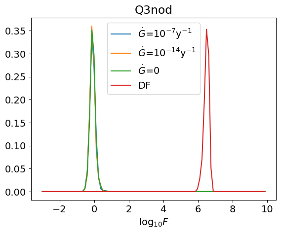
Figure 9: The distribution of $F$ for Q3 d model for different values of $\dot{G}$ in varying-G theory and the dynamical friction of dark matter spike with $\gamma=\frac{3}{2}$.

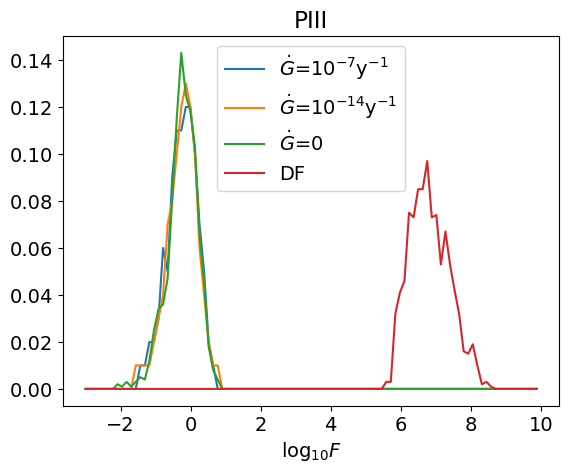
Figure 10: The distribution of $F$ for Q3 d model for different values of $\dot{G}$ in varying-G theory and the dynamical friction of dark matter spike with $\gamma=\frac{3}{2}$.

V Conclusion

In this work, we make a preliminary attempt to distinguish the effect of modified theory of gravity and of environment on GWs. We choose the DF of the dark matter spike with $\gamma=\frac{3}{2}$, and the varying-G theory as an example. Both of these effects have the leading order modification at $-4$ PN order. Since spaceborn GW detectors are much more sensitive to the lower order PN corrections, the characteristic density $\rho_{0}$ can be measured to the level of $10^{-20}\text{kg}/\text{m}^{3}$.

Then with three different models, we use a statistic $F$ to describe the dispersion of the measured $\dot{G}$ for the simulated catalogue. We find that if the deviation is caused by the theory of varying-G, $F$ will be smaller than $10$. On the other hand, if the deviation is cause by dynamical friction, $F$ will be much large, to the level of $10^{6}$.

However, we have made a lot of simplified assumptions in our analysis, which need to be improved in the future work. First, we have assumed $N=10^{6}$ and $\gamma=\frac{3}{2}$ for all the events in DF, and thus $\rho_{0}$ is also fixed. In practice, all these parameters could be different for each event. However, if $\gamma\neq\frac{3}{2}$, the modification will introduce in other order, and will not be confused with varying-G theory. On the other hand, if $\rho_{0}$ also have different values for each event, the dispersion of the distribution of measured $\dot{G}$ will be larger, and thus we will get a larger $F$. So our method is still valid in these more complex cases.

Another problem is that the central value of $\dot{G}$ corresponding to DF is much larger than the current constraint. Thus if we detected such a large result of $\dot{G}$, it could not caused by the modified theory of gravity definitely. This is true for the cases we considered in this work. However, there exist many different kinds of environment effects and modified theories of gravity which could have corrections on the GW at the same order. This method may also be used to distinguish these effects, for which the current constraint is still not accurate enough.

However, if two theories are totally degenerated with each other, which means that for different source parameters, the parameter in the first theory corresponding to a specific value of the parameter in the second theory, Our method will be useless in the distinguishment.