Ref-GS: Directional Factorization for 2D Gaussian Splatting

Abstract

In this paper, we introduce Ref-GS, a novel approach for directional light factorization in 2D Gaussian splatting [10], which enables photorealistic view-dependent appearance rendering and precise geometry recovery. Ref-GS builds upon the deferred rendering of Gaussian splatting and applies directional encoding to the deferred-rendered surface, effectively reducing the ambiguity between orientation and viewing angle. Next, we introduce a spherical Mip-grid to capture varying levels of surface roughness, enabling roughness-aware Gaussian shading. Additionally, we propose a simple yet efficient geometry-lighting factorization that connects geometry and lighting via the vector outer product, significantly reducing renderer overhead when integrating volumetric attributes. Our method achieves superior photorealistic rendering for a range of open-world scenes while also accurately recovering geometry. See our interactive project page.

Figure 1: Our Ref-GS method generates photo-realistic renderings with view-dependent effects while also enabling accurate geometry recovery. The top row shows a comparison of renderings for a scene with specular reflections, along with the recovered normals and mesh. The bottom row demonstrates our successful reconstruction of the geometries of the ‘reflective table center’ in the ‘Garden’ scene [3] and the ‘windshield’ in the ‘Truck’ scene [17], which existing methods typically fail to handle.

1 Introduction

View-dependent effects are a key element in 3D reconstruction and rendering - capturing complex interactions of light in materials such as reflection and refraction - have been studied for decades in forward rendering for computer graphics to enhance realism and visual fidelity in simulations, animations, and visual effects. Recent advances in Neural Radiance Fields (NeRF [26], Mildenhall et al. in 2020) and Gaussian Splatting (GS [13], Kerbl et al. in 2023) have enabled high-fidelity 3D scene reconstruction and novel view synthesis. However, unlike forward rendering in computer graphics, light propagation such as reflection and refraction has received much less attention in neural fields, and significant artifacts in both geometry and rendered images can be observed when reconstructing scenes with complex materials.

This is because NeRF and its follow-ups [2, 3, 38, 45] represent 3D scenes as a collection of emission radiance points and query view-dependent colors using viewing direction, without accounting for the bouncing and bending of light rays as they travel from the light source to the viewing cameras. To tackle this issue, Ref-NeRF [36] take advantage of surface light field rendering [40, 5] and replaces NeRF’s directional parameterization with an integrated reflection encoding, achieving significant improvement in the realism and accuracy of specular reflections. Recent work [41] brings feature grid-based encoding to the directional domain to speed up the efficiency of directional encoding. In the context of 3DGS, directly applying the reflection of the view direction as the view-dependent color query for recent efficient GS representation is problematic, as it independently inherits model orientation and Spherical Harmonics (SH) color for each primitive, resulting in transforming viewing direction can easily be offset during parameter updating. To do so, recent work [43, 46] incorporates smooth regularization and higher-order view-dependent color modeling into the rendering function, achieving promising quality on reflective surfaces. Despite the high rendering quality, they are struggling to provide accurate geometry.

In this paper, we present Ref-GS, a new directional encoding method for 2D Gaussian splatting that leverages deferred rendering and lighting factorization to achieve photorealistic view-dependent effect reconstruction, while preserving accurate geometry. Unlike previous work that treats ray color as the integration of point radiance, We leverage deferred rendering techniques by postponing view-dependent color evaluation until after Gaussian attribute blending and performing directional encoding only on the estimated surface, which efficiently reduces the orientation-viewing ambiguity of Gaussian representations (see Section 4). In addition, we introduce a Mip-grid to capture varying levels of surface roughness, enabling roughness-aware Gaussian shading. Furthermore, spatially varying materials are crucial for modeling open-world scenes; therefore, we propose a simple yet efficient geometry-lighting factorization that connects the geometry and lighting through the vector outer product, significantly lowering renderer overhead for volumetric attribute integration.

Our Ref-GS achieves effective reconstruction of high-frequency reflection and fraction from multi-view images and enables faithful geometry recovery. An extensive evaluation of our approach with both synthetic and real-world scenes demonstrates that Ref-GS produces state-of-the-art renderings of novel views, even compared to implicit methods. Furthermore, our method maintains competitive training times and importantly allows high-quality real-time ($>$ 45 fps) novel view synthesis at $800\times 800$ resolution with a novel deferred mechanism.

Figure 2: Overview of Ref-GS. From left to right: the geometry pass renders the scene properties, including appearance feature $\mathbf{K}$, roughness map $\mathbf{M}$, and normal map $\mathbf{N}$, into buffers via deferred rendering, the lighting pass projects the reflected direction $\omega_{r}$ onto spherical coordinates $(\theta,\phi)$ and featurized by $\operatorname{Sph-Mip}$ encoding for modeling far-field lighting, finally the rendering pass use tensor factorization $\mathbf{s}\circ\mathbf{k}$ to obtain spatially varying view-dependent effects and color each pixel $(u,v)$.

2 Related Work

Our work is closely related to research in novel view synthesis, and reflective and refractive object reconstruction and rendering.

Novel View Synthesis. Novel view synthesis (NVS) focuses on generating novel views from a collection of posed images. A significant achievement in Neural Radiance Fields (NeRF) [26] has been made for realistic NVS, thanks to implicit representations and volumetric rendering. Which has inspired other scene representations, including those for bounded objects [8, 6, 32, 27], unbounded scenes [3, 49, 25, 34], and scenes with high specular reflections and reflective effects [36, 44, 51, 52]. Despite advancements, NeRF-based methods face challenges related to low training and rendering efficiency due to their implicit nature. Recently, 3D Gaussian Splatting (3DGS)[14] has emerged as an alternative 3D representation to NeRF. While 3DGS achieves high-quality novel view synthesis, the reconstructed surface is generally noisy. To address the multi-view geometric inconsistencies in 3DGS, Huang et al. [10] introduced 2D Gaussian Splatting (2DGS), where Gaussian disks are placed on object surfaces and smoothed locally. Our method extends 2DGS, significantly enhancing view-dependent effects and geometry quality.

Reflective Scene Reconstruction and Rendering. Reflective scene reconstruction and rendering has been a challenging task, attracting significant attention. Directional encoding techniques have been explored to improve the modeling of reflections. Ref-NeRF [36] applies Integrated Directional Encoding (IDE) to enhance NeRF’s view-dependent effects but struggles with modeling near-field lighting. To address this limitation, Spec-NeRF [24] introduces Gaussian Directional Encoding, improving the modeling of specular reflections under near-field lighting conditions. Wu et al. [41] proposes Neural Directional Encoding, simulating near-field inter-reflections by tracking light cones within the NeRF model and utilizing a global cubemap filtered by a GGX kernel [37] for reflection modeling. However, these methods rely on large multi-layer perceptrons (MLPs) to represent geometry, resulting in slower training and rendering speeds compared to Gaussian-based representations. Other approaches [21, 23, 20, 44, 48, 12] incorporate indirect lighting. ENVIDR [21] uses a neural renderer to learn physical light interactions through ray tracing, without explicitly formulating the rendering equation. NeRO [23] introduces a lighting representation method using two MLPs and a split-sum approximation to model direct and indirect lighting, enabling high-quality reconstruction of reflective objects. However, NeRO requires extracting geometry from a pre-trained Signed Distance Function (SDF), which takes over 3 hours, resulting in significant inefficiencies. In contrast, recent Gaussian-based methods [11, 42, 35, 15, 53] offer more efficient solutions. For instance, 3iGS [35] uses tensorial factorization [6] to optimize incident illumination, while GaussianShader [11] separately models view-dependent effects, and 3DGS-DR [15] incorporates deferred rendering for reflection modeling. While these methods excel in generating high-quality novel views, they still struggle to model near-field lighting, where environment maps change spatially.

Moreover, concurrent work NU-NeRF [33] simulates reflection and refraction using physics-based ray tracing, improving the reconstruction of objects with fully transparent materials. To better demonstrate our method’s capabilities, we evaluate reconstruction results on real-world scenes with transparent objects.

3 Preliminaries

3.1 Gaussian Splatting

Gaussian Splatting is a recent advance for efficient 3D reconstruction and rendering built upon rasterization. 3DGS and 2DGS are point-based representations that each point associated with geometry attributes (i.e. $\mathbf{\Sigma}\in\mathbb{R}^{3\times 3}$, position $\mu\in\mathbb{R}^{3}$ and opacity $\alpha$) and Spherical Harmonics (SH) appearance attributes $\mathbf{c}$, and the Gaussians are defined in world space centered at $\mu$:

$$\mathcal{G}(\mathbf{x|\mu,\Sigma})=\exp\left(-\frac{1}{2}(\mathbf{x-\mu})^{T}\mathbf{\Sigma}^{-1}(\mathbf{x-\mu})\right)$$ (1)

where the covariance matrix is factorized into a rotation matrix $\bm{R}$ and a scaling matrix $\bm{S}$, to facilitate optimization:

$$\mathbf{\Sigma}=\bm{RSS^{T}R^{T}}$$ (2)

Note that, the surface of the 3D Gaussian is not well defined, leading to noisy surface reconstruction. To address this issue, 2D Gaussian Splatting (2DGS [10]) takes advantage of standard surfel modeling [30, 47, 54] by adopting 2D oriented disks as surface elements and allows high-quality rendering with Gaussian splatting. Specifically, instead of evaluating a Gaussian’s value at the intersection between a pixel ray and a 3D Gaussian [14], 2DGS evaluate Gaussian values at 2D disks and utilizes explicit ray-splat intersection, resulting in a perspective-correct splatting:

$$\mathcal{G}(\mathbf{u})=\exp\left(-\frac{u(\mathbf{r})^{2}+v(\mathbf{r})^{2}}{2}\right)$$ (3)

where $\mathbf{u}=(u(\mathbf{r}),v(\mathbf{r}))$ is the intersection point between ray $\mathbf{r}$ and the primivitve in UV space. Furthermore, each Gaussian primitive has its own view-dependent color $\mathbf{c}$ with SH coefficients. For rendering, Gaussians are sorted according to their centers and composed into pixels with front-to-back alpha blending:

$$\mathbf{c}(\mathbf{r})=\sum_{i=1}\mathbf{c}_{i}\alpha_{i}\mathcal{G}_{i}(\mathbf{u})T_{i}$$ (4)

where $T_{i}$ is approximated accumulated transmittances defined by $\prod_{j=1}^{i-1}(1-\alpha_{j}\mathcal{G}_{j}(\mathbf{u}))$. Note that both 3DGS and 2DGS are forward processes, where scenes are directly projected onto the image plane. Each Gaussian primitive is rendered and lighted in object space before being mapped to screen space. However, forward rendering generally tends to waste a lot of fragment shader runs in scenes with a high depth complexity (multiple primitives cover the same screen pixel) as fragment shader outputs are overwritten.

3.2 Deferred Shading

In 3D computer graphics, deferred shading [7] is a screen-space shading technique designed to significantly reduce the number of shading operations compared to the forward rendering process.

Deferred shading is a technique that defers most intensive rendering operations, such as lighting calculations, to a later stage in the rendering pipeline. This technique involves two main passes. In the first pass, known as the geometry pass, the scene is rendered once to capture various types of geometric information from objects in the scene. These data are stored in a collection of textures called the G-buffer, which contains information such as position vectors, color vectors, normal vectors, and specular values. The G-buffer thus serves as a repository of scene geometry that can be utilized for subsequent, potentially complex, lighting calculations.

In the second pass, referred to as the lighting pass, the G-buffer textures are used to calculate lighting across the scene. A screen-filled quad is rendered, and the lighting for each fragment is computed using the geometric information stored in the G-buffer, iterating over each pixel. This process decouples advanced fragment processing from the initial rendering of each object, allowing lighting calculations to draw directly from the G-buffer textures rather than the vertex shader, with additional input from uniform variables as needed. This allows to maintain the same lighting calculations but optimizes the process by postponing them until after the G-buffer has been populated.

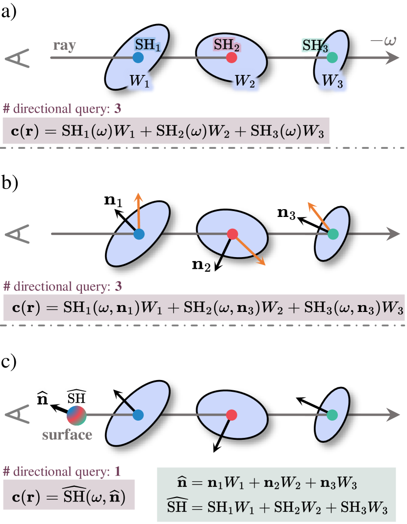
Figure 3: Comparison of directional query in Gaussian Splatting. a) The original 3DGS [14] and 2DGS [10] methods query each primitive’s SH coefficient using the viewing direction, then accumulate view-dependent radiance as the ray color. b) Ref-NeRF [36] and recent GaussianShader [11] utilize the reflection direction transformed by both the viewing and normal directions as the directional query. c) We introduce Gaussian deferred shading by first integrating the SH coefficient and normal as a surface point, then evaluating its view-dependent color.

4 Ambiguity in Directional Query

In prior Gaussian Splatting methods, the diffusion, reflection and refraction components of each primitive are simplified using view-dependent emission radiance, which significantly accelerates the forward rendering process without the needed of per instant lighting evaluation. Then, they optimize the emission radiance together with the geometry jointly through an inverse rendering framework by backpropagating a multi-view photometric loss.

We observe that this modeling suffers from serious representation ambiguities as illustrated in Fig. 3 shows an integration process of three primitives. Consider the integration processing used by vanilla 3D and 2D Gaussian Splatting in (a), it queries view-dependent color using viewing direction, leading to strong bias to diffuse materials and high-frequency irradiance is generally fake by complex primitive overlaying; to handle strong reflection, Ref-NeRF [36] and its follow-ups [21, 23] utilize reflection direction as color query by considering point normal in (b). Unlike the continuous representation in NeRF that neighboring points’ attributes are regularized to each other, Gaussian Splatting treats each point independently. Directly applying reflection direction provides limited gains due to the ambiguity between SH coefficients and the primitive orientation, i.e. transforming viewing direction to reflection direction can be eliminated by the changing in SH coefficient. In practice, since irradiance is independent across primitives and multiple primitives contribute to a target ray, this inherently introduces strong ambiguities, leading to noisy reconstructions.

5 Ref-GS

Our approach aims to reconstruct photorealistic view-dependent effect. The overview of our method is shown in Fig. 2. Specifically, we present a deferred Gaussian splatting to generate a G-buffer (Section 5.1). We then introduce a directional factorization for representing spatially varying view-dependent effects (Section 5.2) and a multi-level spherical feature grid that models far-field lighting (Section 5.3).

5.1 Deferred Gaussian

We now introduce a novel deferred Gaussian Splatting method to address the ambiguity issue discussed in Section 4. Direct volume integration of Gaussian representations can result in blurry view-dependent effects and noisy surfaces due to ambiguity in directional queries. Our solution is to first blend Gaussian attributes, then apply shading, similar to deferred shading. To be specific, we perform alpha blending on primitive attributes (i.e., for the $i^{th}$ Gaussian include diffuse color ${\mathbf{c}_{d}}_{i}\in\mathbb{R}^{3}$, feature $\mathbf{f}_{i}\in\mathbb{R}^{D}$, roughness $\rho_{i}\in[0,1]$) along the rays and convert the attributes into color in image space, as described in Eq. 4 and (c) of Fig. 3. Additionally, the color of each pixel is decomposed into a diffuse component $\mathbf{I}_{d}$ and a specular component, queried by the reflected direction $\omega_{r}\in\mathbb{R}^{3}$ with surface normal $\mathbf{n}\in\mathbb{R}^{3}$. We use the integrated diffuse color $\mathbf{I}_{d}$ directly as the ray’s diffuse component and obtain view-dependent effects at each pixel through a shader $f_{\Theta}$, conditioned on the spatial feature $\mathbf{K}\in\mathbb{R}^{H\times W\times D}$ and the directional feature $\mathbf{S}\in\mathbb{R}^{H\times W\times C}$:

$$\mathbf{I}=\mathbf{I}_{d}+f_{\Theta}(\mathbf{S},\mathbf{K}\otimes\mathbf{S})$$ (5)

where $\otimes$ denotes the per-pixel outer product, obtaining the high-dimensional intermediate tensor with the shape of $H\times W\times(D\times C)$.

Note that the feature $\mathbf{K}$ represents the expected feature of each pixel and is obtained by splatting per-primitive features $\mathbf{f}_{i}$ using Eq. 4. Similarly, we generate the roughness map $\mathbf{M}$ corresponding to $\rho_{i}$ and the normal map $\mathbf{N}$. In practice, we treat ${\mathbf{M},\mathbf{N},\mathbf{K}}$ as a G-buffer and pass it a standard rasterization render for shading.

5.2 Directional Factorization

In essence, the key to modeling view-dependent effects is accurately capturing spatially varying near- and far-field inter-reflections. Prior methods [11, 15, 28] often rely on a global 2D environment map for far-field lighting, assuming all light sources are at an infinite distance. Other methods [36, 35] only model direct lighting. These assumptions are insufficient for reconstructing surfaces under near-field lighting, especially in scenes where light sources or objects are close to the target object.

Inspired by TensoRF [6], we propose a low-rank tensor factorization $\mathbf{s}\circ\mathbf{k}$ to represent spatio-angular view-dependent effects, where $\circ$ denotes the outer product. As illustrated in Fig. 2, we connect the spatial feature vector $\mathbf{k}\in\mathbb{R}^{D}$ and directional feature vector $\mathbf{s}\in\mathbb{R}^{C}$ using a simple vector outer product to form a block matrix, which is then flattened into a 1D vector and fed into a lightweight MLP decoder for final color prediction. The outer product of spatial feature $\mathbf{k}$ and directional feature $\mathbf{s}$ enables decomposition of geometry and lighting, while effectively capturing essential information such as global lighting, shadows, and self-occlusion.

Our factorization-based model is simple yet effective for representing spatially varying view-dependent effects in complex reflective scenes, enhancing both novel view synthesis and surface reconstruction. Additionally, this factorization reduces the feature channels for each Gaussian primitive, significantly lowering the computational overhead in volume rendering and scene representation.

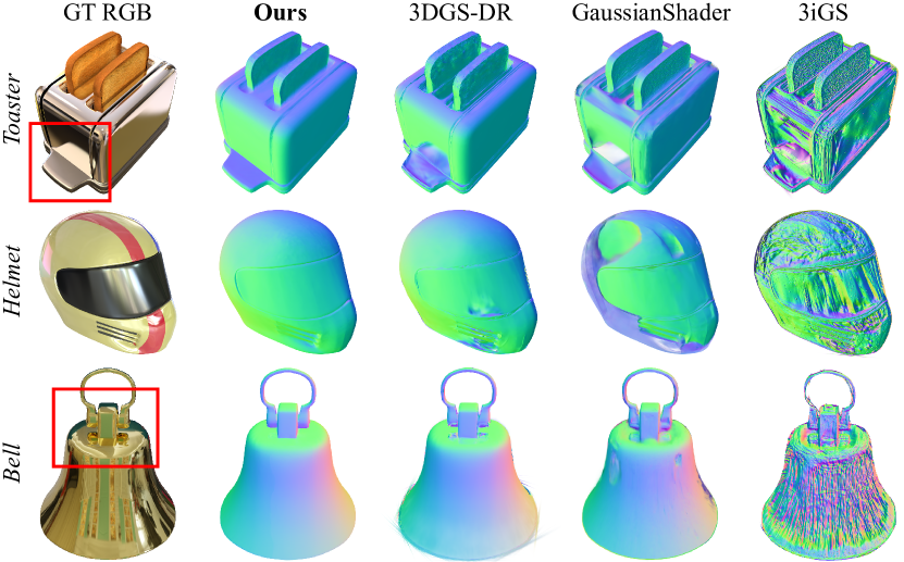
Figure 4: Visualized estimated surface normal results synthetic datasets [36, 23]. Compared to existing Gaussian-based methods, our method has more accurate surface reconstruction for shiny objects with inter-reflections, as depicted for this ‘Toaster’ and ‘Bell’ scenes.

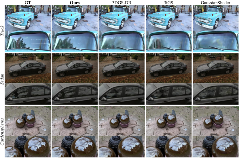
Figure 5: Qualitative comparisons of test-set views of real-world scenes. Notice the high-frequency reflections rendered by our model, including sharp details of the tree branches and buildings reflected in the sphere.

5.3 Far-field Lighting

We now present a novel $\operatorname{Sph-Mip}$ encoding for modeling high-frequency far-field lighting, using a learnale multi-level spherical feature grid, named $\operatorname{Sph-Mip}$ grid.

We utilize a longitude-latitude lattice (Long.-Lat.) to distribute feature points on a spherical surface and unfold them into a 2D feature grid for efficient indexing. Given the G-buffer $\{\mathbf{M},\mathbf{N},\mathbf{K}\}$, the normal $\mathbf{n}=\mathbf{N}(u,v)$, roughness $\rho=\mathbf{M}(u,v)$ for the pixel $(u,v)$, we have:

$$\mathbf{s}=\operatorname{Sph-Mip}(\omega_{r},\rho,\mathcal{M})$$ (6)

where $\omega_{r}$ denotes the reflection direction reflected by the surface normal $\mathbf{n}$ and viewing direction $\omega_{i}$.

Note that, as shown in Fig. 2, the $\operatorname{Sph-Mip}$ grid is three-dimensional, the directional coordinates $(\theta,\phi)$ correspond to the XY axes of the grid, while the Z-axis represents the roughness $\rho$ variance. Given reasterized buffers, we first calculate its corresponding spherical coordinates $(\theta,\phi)$ for each pixel by:

$$\theta =\text{arccos}\left(\frac{\omega_{r}^{z}}{\sqrt{{\omega_{r}^{x}}^{2}+{\omega_{r}^{y}}^{2}+{\omega_{r}^{z}}^{2}}}\right)\in\left[0,\pi\right]$$ (7)

$$\phi =\text{arctan2}\left(\frac{{\omega_{r}^{y}}}{{\omega_{r}^{x}}}\right)\in\left[-\pi,\pi\right]$$

Then, given the surface roughness $\rho$, we interpolate features along the roughness dimension. In practice, we resize the grids at different levels to the same resolution during the feature query, facilitating efficient three-dimensional interpolation using trilinear interpolation with the coordinates $(\theta,\phi,\rho)$ in the fragment shader.

For the mipmap resolution, we define the base level $\mathcal{M}^{L_{0}}$ at the highest resolution of $H_{\mathcal{M}}\times W_{\mathcal{M}}\times C$, where $H_{\mathcal{M}}$, $W_{\mathcal{M}}$, and $C$ represent the height, width, and number of channels, respectively. While the resolution for other levels ($\mathcal{M}^{L_{i}},i={1,2,\dots,N}$) is divided by $2\times$ along the height and width dimensions.

6 Experiments and Results

	Shiny Blender							Shiny Real
	Car	Ball	Helmet	Teapot	Toaster	Coffee	Avg.	Garden	Sedan	Toycar	Avg.
PSNR$\uparrow$
Ref-NeRF [36]	30.41	29.14	29.92	45.19	25.29	33.99	32.32	22.01	25.21	23.65	23.62
NeRO [23]	25.53	30.26	29.20	38.70	26.46	28.89	29.84	—	—	—	—
ENVIDR [21]	28.46	38.89	32.73	41.59	26.11	29.48	32.88	21.47	24.61	22.92	23.00
3DGS [14]	27.24	27.69	28.32	45.68	20.99	32.32	30.37	21.75	26.03	23.78	23.85
GaussianShader [11]	27.51	29.02	28.73	43.05	22.86	31.34	30.42	21.74	24.89	23.76	23.46
3iGS [35]	27.52	26.82	28.08	46.05	22.71	32.64	30.64	21.96	26.59	23.75	24.10
3DGS-DR [15]	30.43	33.44	31.49	47.00	26.69	34.61	33.94	21.52	26.32	23.57	23.80
Ours	30.94	36.10	33.40	46.69	27.28	34.38	34.80	22.48	26.63	24.20	24.44
SSIM$\uparrow$
Ref-NeRF [36]	0.949	0.956	0.955	0.995	0.910	0.972	0.956	0.584	0.720	0.633	0.646
NeRO [23]	0.949	0.974	0.971	0.995	0.929	0.956	0.962	—	—	—	—
ENVIDR [21]	0.961	0.991	0.980	0.996	0.939	0.949	0.969	0.561	0.707	0.549	0.606
3DGS [14]	0.930	0.937	0.951	0.996	0.895	0.971	0.947	0.571	0.771	0.637	0.660
GaussianShader [11]	0.930	0.954	0.955	0.995	0.900	0.969	0.951	0.576	0.728	0.637	0.647
3iGS [35]	0.930	0.933	0.951	0.996	0.909	0.972	0.948	0.557	0.789	0.626	0.657
3DGS-DR [15]	0.962	0.979	0.971	0.997	0.942	0.976	0.971	0.570	0.773	0.635	0.659
Ours	0.961	0.981	0.975	0.997	0.950	0.973	0.973	0.607	0.783	0.656	0.682
LPIPS$\downarrow$
Ref-NeRF [36]	0.051	0.307	0.087	0.013	0.118	0.082	0.110	0.251	0.234	0.231	0.239
NeRO [23]	0.074	0.094	0.050	0.012	0.089	0.110	0.072	—	—	—	—
ENVIDR [21]	0.049	0.067	0.051	0.011	0.116	0.139	0.072	0.263	0.387	0.345	0.332
3DGS [14]	0.047	0.161	0.079	0.007	0.126	0.078	0.083	0.248	0.206	0.237	0.230
GaussianShader [11]	0.045	0.148	0.088	0.012	0.111	0.085	0.082	0.274	0.259	0.239	0.257
3iGS [35]	0.045	0.166	0.073	0.006	0.098	0.077	0.077	0.252	0.190	0.251	0.231
3DGS-DR [15]	0.034	0.104	0.050	0.006	0.083	0.076	0.059	0.251	0.208	0.249	0.236
Ours	0.034	0.098	0.045	0.006	0.070	0.082	0.056	0.242	0.196	0.236	0.224

Table 1: Quantitative NVS comparisons on Shiny Blender and Shiny Real datasets [36]. Our method is comparable with both Gaussian-based methods and prior reflective object reconstruction methods. ‘Gardenspheres’ is abbreviated as ‘Garden’.

6.1 Datasets

We evaluate our method on several synthetic and real-world datasets. For the synthetic datasets, we evaluate our model on NeRF Synthetic [26], which contains scenes of complex geometries with realistic non-Lambertian materials. Similarly, we evaluate our model on reflective objects using Shiny Blender [36] and Glossy Synthetic [23]. For the real-world datasets, we use Shiny Real dataset captured from [36], as well as scenes with reflections from Mip-NeRF360 [3] and Tanks $\&$ Temples [17]. Additionally, we use Glass $\&$ Ball [4], which contains refractive objects with unknown geometry, to show the generalization ability of our method for diverse materials.

Figure 6: Comparison results on refractive scenes. Normal reconstruction and rendering results on real scenes from Glass $\&$ Ball [4]. Our method performs significantly better than 3DGS-DR [15] and 3iGS [35].

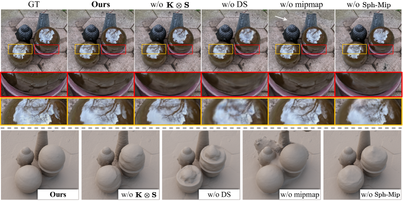
Figure 7: Qualitative ablation on the ‘Gardenspheres’ scene [36]. Using the G-buffer instead of $\operatorname{Sph-Mip}$ (i.e., w/o $\operatorname{Sph-Mip}$) or without deferred shading (i.e., w/o DS), sharp details, such as tree branches reflected in the sphere, are not accurately reconstructed. It is necessary to use multi-level spherical feature grid strategies (i.e., w/o mipmap), otherwise rough surfaces will fail to be reconstructed and artifacts will appear during rendering. Additionally, directional factorization (i.e., w/o $\mathbf{K}\otimes\mathbf{S}$) is essential for modeling near-field inter-reflections.

6.2 Baselines and metrics

We compare our method with the following baselines: Ref-NeRF [36], a NeRF-based method focusing on reflective objects rendering; SDF-based methods including ENVIDR [21] and NeRO [23], top-performing implicit methods for reconstructing reflective objects; and Gaussian-based methods such as GaussianShader [11], 3iGS [35] and 3DGS-DR [15]. We trained these models based on their public codes and configurations. Evaluation metrics for rendering quality include PSNR, SSIM [39], and LPIPS [50]. Additionally, we use Mean Angular Error in degrees (MAE^∘) to evaluate the normal accuracy.

6.3 Implementation Details

All experiments are conducted on a single Tesla V100 GPU with 32GB of VRAM. The parameters to be optimized include the MLP $f_{\Theta}$, the mipmap $\mathcal{M}$ and each 2D Gaussian’s parameters (e.g. the feature $\mathbf{f}_{i}\in\mathbb{R}^{4}$). Following the approach in [10], we optimize these parameters using differentiable splatting and gradient-based backpropagation. Optimization was performed over 30,000 iterations using the Adam optimizer [16]. We implement our $\operatorname{Sph-Mip}$ using PyTorch [29] framework, and employ the Nvdiffrast [19] library for efficient mipmap querying. The shape of the base level of the mipmap $\mathcal{M}^{L_{0}}$ in $\operatorname{Sph-Mip}$ encoding is empirically set to $H_{\mathcal{M}}=512,W_{\mathcal{M}}=1024,C=16$, and the number of levels is $N=9$. For our implicit representation of the specluar color prediction, we use a lightweight MLP with 1 hidden layers of size 256. We use the ReLU activation function. We propose to train our model with the same loss function $\mathcal{L}$ as 2DGS [10].

6.4 Comparisons

Quantitative results on synthetic datasets are reported in Tab. 1 and Tab. 2, where high-quality reflection modeling relies on accurate normal estimation, as shown in Fig. 4. Furthermore, we report the training and rendering speeds (tested) of our model on the same hardware in Tab. 4, comparing it with existing Gaussian-based methods. Our method achieves a balance between quality and training speed. Although the speed of our model is not as fast as 3DGS [14], it remains competitive and achieves real-time rendering speeds.

To demonstrate the effectiveness of our method in real-world scenes, rather than just small objects, we evaluated our renderings on the Shiny Real dataset from Ref-NeRF [36] as shown in Tab. 1 and Fig. 5. Furthermore, the qualitative results in Fig. 6 show that for real-world scenes with refractive objects, our model outperforms 3iGS [35] and 3DGS-DR [15] on the Glass $\&$ Ball dataset from Eikonal Fields [4].

6.5 Ablation Studies

	NeRF Synthetic			Glossy Synthetic			ShinyB
	PSNR$\uparrow$	SSIM$\uparrow$	LPIPS$\downarrow$	PSNR$\uparrow$	SSIM$\uparrow$	LPIPS$\downarrow$	MAE∘$\downarrow$
Ref-NeRF [36]	31.29	0.947	0.058	27.50	0.927	0.100	18.38
ENVIDR [21]	28.13	0.953	0.068	29.58	0.952	0.057	4.61
3DGS [14]	33.30	0.969	0.030	26.50	0.917	0.092	—
GShader [11]	31.48	0.960	0.042	27.54	0.922	0.087	10.93
3iGS [35]	33.60	0.970	0.029	26.39	0.913	0.089	15.47
3DGS-DR [15]	31.02	0.962	0.047	29.78	0.954	0.057	2.43
GS-ROR [53]	—	—	—	29.70	0.956	—	7.23
Ours	33.20	0.966	0.036	30.59	0.957	0.058	2.21

Table 2: Quantitative NVS comparisons on NeRF Synthetic [26] and Glossy Synthetic [23] datasets. Normal reconstruction quality on the Shiny Blender (ShinyB) [36] dataset evaluated by MAE^∘. GaussianShader [11] is abbreviated as GShader.

	PSNR$\uparrow$	SSIM$\uparrow$	LPIPS$\downarrow$	MAE∘$\downarrow$
w/o $\operatorname{Sph-Mip}$	29.95	0.943	0.090	3.61
w/o mipmap	30.12	0.945	0.091	5.12
w/o DS	31.79	0.957	0.062	2.57
w/o $\mathbf{K}\otimes\mathbf{S}$	33.37	0.966	0.051	2.38
Ours	34.00	0.969	0.046	2.21

Table 3: Ablation study of our model on the synthetic datasets.

We now perform ablation studies on the Shiny Blender [36] and NeRF Synthetic [26] datasets. Tab. 3 reports quantitative results for deferred shading, $\operatorname{Sph-Mip}$ encoding, and directional factorization. Fig. 7 shows ablation comparisons for novel view synthesis and surface reconstruction.

Sph-Mip. We first analyze the effect of the $\operatorname{Sph-Mip}$ by directly feeding G-buffer components to the decoding MLP: $f_{\Theta}(\mathbf{M},\mathbf{N},\mathbf{d})$, where $\mathbf{d}\in\mathbb{R}^{H\times W\times 3}$ is the view directions. As shown in Fig. 7 and Tab. 3, compared to directly using the G-buffer as input, our $\operatorname{Sph-Mip}$ encoding effectively models high-frequency view-dependent appearance.

Mipmap. To verify the effectiveness of the multi-level spherical feature grid strategies, we replace the mipmap $\mathcal{M}$ with a 2D feature map of the same shape as the base level of the mipmap $\mathcal{M}^{L_{0}}$ (i.e., w/o mipmap). Fig. 7 shows that the method without mipmap fails to recover accurate geometry and produces artifacts when rendering rough surfaces, primarily because real-world scenes typically do not consist of a single material.

Deferred Shading. We ablate deferred shading (i.e., w/o DS) by applying the standard volume rendering. As shown in Fig. 7, deferred shading provides more accurate specular reflections and better surface reconstruction quality.

Directional Factorization. We study the proposed directional factorization (i.e., w/o $\mathbf{K}\otimes\mathbf{S}$). We directly used the directional feature $\mathbf{S}$ as input to the shader: $f_{\Theta}(\mathbf{S})$. As shown in Fig. 7, inter-reflections cannot be reconstructed using only the far-field feature $\mathbf{S}$.

	Rendering Speed	Train Time
3DGS [14]	1.00$\times$	1.00$\times$
GaussianShader [11]	$0.17\times$	11.05$\times$
3iGS [35]	$0.44\times$	2.07$\times$
3DGS-DR [15]	$0.93\times$	3.25$\times$
Ours	$0.37\times$	2.63$\times$

Table 4: Comparisons on training and rendering (test) speed. We consider the 3DGS [14] as a baseline and normalise the speed. With our GPU device, 3DGS takes about 14.5 min for training, and achieves 125 FPS for rendering.

7 Conclusion

We have presented Ref-GS to address view-dependent effects in 2D Gaussian Splatting, enabling photorealistic rendering and precise geometry recovery for open-world scenes. Our technical contribution is a novel deferred Gaussian rendering pipeline that integrates a spherical Mip-grid to efficiently represent surface roughness and employs a geometry-lighting factorization to explicitly connect geometry and lighting through the vector outer product.

Supplementary Material

This supplementary material provides additional information and experiment results pertaining to the main paper including detailed descriptions of the training process, and more visual results to complement the experiments reported in the main manuscript.

For more information regarding the method, we highly encourage readers to watch our video provided in the supplemental webpage, where our method produces results with better specular reflection reconstruction.

Appendix A Implementation Details

For training, we use the PyTorch [29] framework and train on a single Tesla V100 with 32GB of memory. Our code is build upon the 2D Gaussian Splatting (2DGS) [10] codebase. For real scenes, we propose using the same spherical domain strategy as 3DGS-DR [15] to train our model for a fair evaluation. This approach can reduce background interference during training. Background objects, captured from only limited viewpoints, exhibit similar behavior to reflective objects, which interferes with the fitting of our $\operatorname{Sph-Mip}$.

A.1 Network

The goal of the shallow MLP $f_{\Theta}$ is is to non-linearly map the directional feature $\mathbf{S}\in\mathbb{R}^{H\times W\times 16}$ produced by the $\operatorname{Sph-Mip}$ encoding and the high-dimensional intermediate tensor $\mathbf{K}\otimes\mathbf{S}$ has a shape of $H\times W\times 64$. Our MLP accepts an input having $16+64$ feature dimensions. The input is fed into a 2-layer MLP with 256 neurons per hidden layer in them followed by ReLU activation functions. The output is fed into a output head predicts the view-dependent radiance with a exponential function output layer. Finally, we apply gamma tone mapping [1] $\gamma(\cdot)$ to convert the colors into the sRGB space before calculating the rendering loss:

$$\mathbf{I}=\gamma(\mathbf{I}_{d}+f_{\Theta}(\mathbf{S},\mathbf{K}\otimes\mathbf{S}))$$ (8)

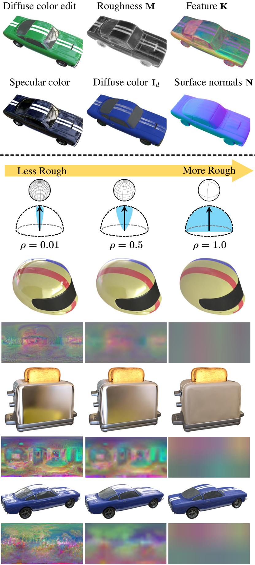
Figure 8: Visualization of the Scene Decompositions and Material Editing. Our model decomposes the appearance of synthetic scenes into interpretable components. Ref-GS effectively separates view-independent diffuse colors and view-dependent specular colors from multi-view training images. Furthermore, we can edit the diffuse color of the car without affecting the specular reflections on its glossy surface (top row). By modifying roughness $\rho$, we can obtain directional feature $\mathbf{s}$ at different levels can be obtained through $\operatorname{Sph-Mip}$ interpolation (bottom row).

A.2 Optimization

The per-Gaussian position $\mu\in\mathbb{R}^{3}$, scale $s\in\mathbb{R}^{2}$ and covariance as rotation $q\in\mathbb{R}^{4}$, opacity $\alpha\in\mathbb{R}$, diffuse color $\mathbf{c}_{d}\in\mathbb{R}^{3}$, roughness $\rho\in[0,1]$, feature $\mathbf{f}\in\mathbb{R}^{4}$ are optimized together with the network weights for the base MLP and the output head for view-dependent radiance. We use the Adam [16] optimizer with default parameters. Further, we follow the default splitting and pruning schedule proposed by the original 2DGS.

A.3 Losses

We have multiple loss terms in our training pipeline that are mainly adapted from 2DGS that we will briefly outline them and their weighting here. As in 2DGS, we use $\mathcal{L}_{1}$ loss and D-SSIM [39] loss for supervising RGB color, with $\lambda=0.2$:

$$\mathcal{L}_{\text{rgb}}=(1-\lambda)\mathcal{L}_{1}+\lambda\mathcal{L}_{\text{D-SSIM}}.$$ (9)

Following 2DGS, depth distortion loss and normal consistency loss are adopted to refine the geometry property of the 2DGS representation of the scene.

$$\mathcal{L}_{\text{d}}=\sum_{i,j}\omega_{i}\omega_{j}|z_{i}-z_{j}|\hskip 14.22636pt\mathcal{L}_{n}=\sum_{i}\omega_{i}(1-\mathbf{n}_{i}^{\top}\mathbf{\widehat{N}})$$ (10)

Here, $\omega_{i}$ represents the blending weight of the $i^{th}$ intersection. $z_{i}$ denotes the depth of the intersection points. $\mathbf{n}_{i}$ is the normal of the splat facing the camera. $\mathbf{\widehat{N}}$ is the normal estimated by the gradient of the depth map. The total loss is given as:

$$\mathcal{L}=\mathcal{L}_{\text{rgb}}+\lambda_{d}\mathcal{L}_{\text{d}}+\lambda_{n}\mathcal{L}_{\text{n}}$$ (11)

We empirically set $\lambda_{d}=100$, $\lambda_{n}=0.05$.

Appendix B Limitations

While our approach demonstrates effective performance with a lightweight MLP for final color prediction, it results in slower rendering speeds compared to 2DGS and is challenging to integrate into standard CG rendering engines due to its reliance on a neural decoder. However, conversion techniques like textured mesh baking can facilitate integration and benefit from our reconstruction pipeline’s thin surface modeling and rendering capabilities.

Appendix C Additional Results

In this section, we present additional visual results to demonstrate the capability of Ref-GS in reconstructing and rendering glossy surfaces, showcasing superior visual quality and accurate predicted normals for specular reflections across diverse scenes in the proposed dataset.

	Shiny Blender
	Car	Ball	Helmet	Teapot	Toaster	Coffee	Avg.
	MAE∘$\downarrow$
NVDiffRec [28]	11.78	32.67	21.19	5.55	16.04	15.05	17.05
Ref-NeRF [36]	14.93	1.55	29.48	9.23	42.87	12.24	18.38
ENVIDR [21]	7.10	0.74	1.66	2.47	6.45	9.23	4.61
GaussianShader [11]	14.05	7.03	9.33	7.17	13.08	14.93	10.93
GS-IR [22]	28.31	25.79	25.58	15.35	33.51	15.38	23.99
RelightGS [9]	26.02	22.44	19.63	9.21	28.17	13.39	19.81
3iGS [35]	11.79	31.78	16.72	2.61	21.12	8.80	15.47
3DGS-DR [15]	2.32	0.85	1.67	0.53	6.99	2.21	2.43
GS-ROR [53]	11.98	0.92	4.10	5.88	8.24	12.24	7.23
Ours	2.02	1.05	1.99	0.69	3.92	3.61	2.21

Table 5: Quantitative Mean Angular Error in degrees (MAE^∘$\downarrow$) of individual scenes on Shiny Blender [36] dataset. Red, Orange, and Yellow indicate the first, second, and third best performing methods for each scene.

C.1 Shiny Blender Dataset

Tab. 5 provides the results on normal estimation for all scenes on Shiny Blender [36] dataset. For 3iGS [35], we use grad normals derived from the rendered depth map for evaluation.

C.2 Glossy Synthetic Dataset

We present the novel view synthesis results on the Glossy Synthetic [23] dataset. The quantitative evaluation in terms of Peak Signal-to-Noise Ratio (PSNR), Structural Similarity Index Measure (SSIM) [39], and Learned Perceptual Image Patch Similarity (LPIPS) [50]. is present in Tab. 6. Our approach outperforms the existing Gaussian-based methods [15, 53, 35, 11] on most scenes.

	Glossy Synthetic
	Bell	Cat	Luyu	Potion	Tbell	Teapot	Avg.
	PSNR$\uparrow$
Ref-NeRF [36]	30.02	29.76	25.42	30.11	26.91	22.77	27.50
NeRO [23]	—	—	—	—	—	—	—
ENVIDR [21]	30.88	31.04	28.03	32.11	28.64	26.77	29.58
3DGS [14]	25.11	31.36	26.97	30.16	23.88	21.51	26.50
GaussianShader [11]	28.07	31.81	27.18	30.09	24.48	23.58	27.54
3iGS [35]	25.60	30.93	27.17	29.50	23.94	21.17	26.39
3DGS-DR [15]	31.84	33.39	28.62	31.74	27.65	25.44	29.78
GS-ROR [53]	31.53	31.72	28.53	30.51	29.48	26.41	29.70
Ours	31.70	33.15	29.46	32.64	30.08	26.47	30.59
	SSIM$\uparrow$
Ref-NeRF [36]	0.941	0.944	0.901	0.933	0.947	0.897	0.927
NeRO [23]	0.965	0.962	0.914	0.950	0.968	0.977	0.956
ENVIDR [21]	0.954	0.965	0.931	0.960	0.947	0.957	0.952
3DGS [14]	0.908	0.959	0.916	0.938	0.900	0.881	0.917
GaussianShader [11]	0.919	0.961	0.914	0.936	0.898	0.901	0.922
3iGS [35]	0.898	0.960	0.916	0.936	0.896	0.869	0.913
3DGS-DR [15]	0.964	0.976	0.938	0.957	0.948	0.939	0.954
GS-ROR [53]	0.969	0.967	0.938	0.950	0.965	0.947	0.956
Ours	0.965	0.973	0.946	0.957	0.956	0.944	0.957
	LPIPS$\downarrow$
Ref-NeRF [36]	0.102	0.104	0.098	0.084	0.114	0.098	0.100
NeRO [23]	0.056	0.052	0.072	0.084	0.046	0.028	0.056
ENVIDR [21]	0.054	0.049	0.059	0.072	0.069	0.041	0.057
3DGS [14]	0.104	0.062	0.064	0.093	0.125	0.102	0.092
GaussianShader [11]	0.098	0.056	0.064	0.088	0.122	0.091	0.087
3iGS [35]	0.104	0.057	0.064	0.089	0.119	0.103	0.089
3DGS-DR [15]	0.044	0.039	0.052	0.073	0.070	0.062	0.057
GS-ROR [53]	—	—	—	—	—	—	—
Ours	0.049	0.041	0.046	0.076	0.073	0.064	0.058

Table 6: Quantitative results of individual scenes on Glossy Synthetic [23] dataset. Red, Orange, and Yellow indicate the first, second, and third best performing methods for each scene.

C.3 Glossy Real Dataset

We present the geometry reconstruction results on the Glossy Real [23] dataset to further validate the robustness and accuracy of our approach. We visualized the reconstruction results as shown in Fig. 9.

For a more comprehensive view of our method’s performance, please refer to the videos provided on the supplemental webpage.

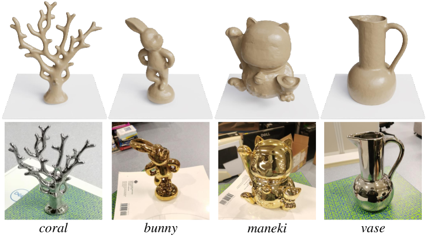
Figure 9: Images, ground-truth and reconstructed surfaces of the Glossy Real [23] dataset.

C.4 NeRF Synthetic Dataset

Quantitative results on the NeRF Synthetic [26] dataset are reported in Tab. 7. Our approach achieves numerically and visually comparable results with Gaussian-based methods [15, 53, 35, 11], demonstrating the effectiveness of our method in rendering general objects.

	NeRF Synthetic
	Chair	Drums	Lego	Mic	Materials	Ship	Hotdog	Ficus	Avg.
	PSNR$\uparrow$
NeRF [26]	33.00	25.01	32.54	32.91	29.62	28.65	36.18	30.13	31.01
Ref-NeRF [36]	33.98	25.43	35.10	33.65	27.10	29.24	37.04	28.74	31.29
VolSDF [45]	30.57	20.43	29.46	30.53	29.13	25.51	35.11	22.91	27.96
ENVIDR [21]	31.22	22.99	29.55	32.17	29.52	21.57	31.44	26.60	28.13
3DGS [14]	35.82	26.17	35.69	35.34	30.00	30.87	37.67	34.83	33.30
GaussianShader [11]	33.70	25.50	32.99	34.07	28.87	28.37	35.29	33.05	31.48
3iGS [35]	35.59	26.75	35.94	36.01	30.00	31.12	37.98	35.40	33.60
3DGS-DR [15]	35.60	25.31	32.94	31.97	29.65	29.07	35.58	28.03	31.02
Ours	34.66	26.33	36.26	35.76	30.99	29.67	37.39	34.52	33.20
	SSIM$\uparrow$
NeRF [26]	0.967	0.925	0.961	0.980	0.949	0.856	0.974	0.964	0.947
Ref-NeRF [36]	0.974	0.929	0.975	0.983	0.921	0.864	0.979	0.954	0.947
VolSDF [45]	0.949	0.893	0.951	0.969	0.954	0.842	0.972	0.929	0.932
ENVIDR [21]	0.976	0.930	0.961	0.984	0.968	0.855	0.963	0.987	0.953
3DGS [14]	0.987	0.954	0.983	0.991	0.960	0.907	0.985	0.987	0.969
GaussianShader [11]	0.980	0.945	0.972	0.989	0.951	0.881	0.980	0.982	0.960
3iGS [35]	0.987	0.955	0.983	0.992	0.961	0.908	0.986	0.989	0.970
3DGS-DR [15]	0.986	0.946	0.978	0.987	0.958	0.894	0.982	0.963	0.962
Ours	0.985	0.952	0.982	0.991	0.964	0.890	0.984	0.982	0.966
	LPIPS$\downarrow$
NeRF [26]	0.046	0.091	0.050	0.028	0.063	0.206	0.121	0.044	0.081
Ref-NeRF [36]	0.029	0.073	0.025	0.018	0.078	0.158	0.028	0.056	0.058
VolSDF [45]	0.056	0.119	0.054	0.191	0.048	0.191	0.043	0.068	0.096
ENVIDR [21]	0.031	0.080	0.054	0.021	0.045	0.228	0.072	0.010	0.068
3DGS [14]	0.012	0.037	0.016	0.006	0.034	0.106	0.020	0.012	0.030
GaussianShader [11]	0.019	0.045	0.026	0.009	0.046	0.148	0.029	0.017	0.042
3iGS [35]	0.012	0.036	0.015	0.005	0.034	0.102	0.019	0.010	0.029
3DGS-DR [15]	0.014	0.055	0.026	0.028	0.038	0.129	0.033	0.055	0.047
Ours	0.013	0.044	0.016	0.009	0.042	0.127	0.021	0.017	0.036

Table 7: Quantitative results of individual scenes on NeRF Synthetic [26] dataset. Red, Orange, and Yellow indicate the first, second, and third best performing methods for each scene.

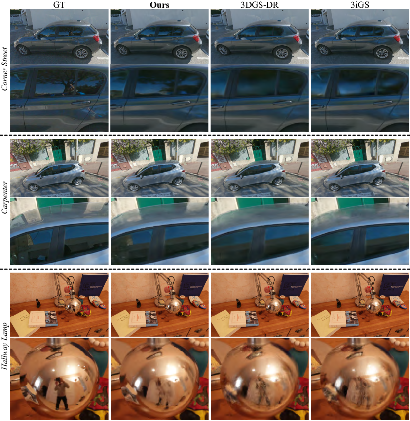
Figure 10: Additional results for intermediate component visualizations of our approach compared to 3DGS-DR [15] and 3iGS [35] on the Rodriguez et al. [31] and Kopanas et al. [18] datasets; zoom in to see the difference. (Corner Street, 1st row) Our approach effectively simulates realistic reflections on the car body and windshield. (Carpenter, 2nd row) Reflections of distant scenes on the car roof are rendered with impressive accuracy. (Hallway Lamp, 3rd row) High-frequency details are well-preserved, enabling the realistic depiction of near-field content, including precise reflections.

C.5 Additional Results on Real-World Captures

In this section, we extend the evaluation of our proposed method to include its performance on Rodriguez et al. [31] and Kopanas et al. [18] datasets. The qualitative comparison in Fig. 10 shows that Ref-GS extends well to real scenes, producing clearer specular reflections of the complex real-world environments compared to the existing Gaussian-based methods.

C.6 Scene Decompositions and Editing

Fig. 8 illustrates the rendering decomposition results of the scene. For reflective objects exhibiting strong specular effects, our approach can effectively decompose both the view-independent diffuse color and view-dependent specular color. Furthermore, the predicted material properties (e.g., roughness $\rho$) and far-field lighting $\mathcal{M}$ are also very reasonable. Additionally, we can plausibly modify the roughness of the scenes by adjusting the $\rho$ values.

C.7 Supplementary Video Results

For a more comprehensive understanding of the performance of our approach, please refer to the supplementary videos provided. Additionally, we have created an interactive webpage to vividly showcase the capabilities of our approach.

References

- Anderson et al. [1996] Matthew Anderson, Ricardo Motta, Srinivasan Chandrasekar, and Michael Stokes. Proposal for a standard default color space for the internet—srgb. In Color and imaging conference, pages 238–245. Society of Imaging Science and Technology, 1996.
- Barron et al. [2021] Jonathan T Barron, Ben Mildenhall, Matthew Tancik, Peter Hedman, Ricardo Martin-Brualla, and Pratul P Srinivasan. Mip-nerf: A multiscale representation for anti-aliasing neural radiance fields. In Proceedings of the IEEE/CVF international conference on computer vision, pages 5855–5864, 2021.
- Barron et al. [2022] Jonathan T Barron, Ben Mildenhall, Dor Verbin, Pratul P Srinivasan, and Peter Hedman. Mip-nerf 360: Unbounded anti-aliased neural radiance fields. In Proceedings of the IEEE/CVF conference on computer vision and pattern recognition, pages 5470–5479, 2022.
- Bemana et al. [2022] Mojtaba Bemana, Karol Myszkowski, Jeppe Revall Frisvad, Hans-Peter Seidel, and Tobias Ritschel. Eikonal fields for refractive novel-view synthesis. In ACM SIGGRAPH 2022 Conference Proceedings, pages 1–9, 2022.
- Chen et al. [2018] Anpei Chen, Minye Wu, Yingliang Zhang, Nianyi Li, Jie Lu, Shenghua Gao, and Jingyi Yu. Deep surface light fields. 2018.
- Chen et al. [2022] Anpei Chen, Zexiang Xu, Andreas Geiger, Jingyi Yu, and Hao Su. Tensorf: Tensorial radiance fields. In European conference on computer vision, pages 333–350. Springer, 2022.
- Deering et al. [1988] Michael Deering, Stephanie Winner, Bic Schediwy, Chris Duffy, and Neil Hunt. The triangle processor and normal vector shader: a vlsi system for high performance graphics. Acm siggraph computer graphics, 22(4):21–30, 1988.
- Fridovich-Keil et al. [2022] Sara Fridovich-Keil, Alex Yu, Matthew Tancik, Qinhong Chen, Benjamin Recht, and Angjoo Kanazawa. Plenoxels: Radiance fields without neural networks. In Proceedings of the IEEE/CVF conference on computer vision and pattern recognition, pages 5501–5510, 2022.
- Gao et al. [2023] Jian Gao, Chun Gu, Youtian Lin, Hao Zhu, Xun Cao, Li Zhang, and Yao Yao. Relightable 3d gaussian: Real-time point cloud relighting with brdf decomposition and ray tracing. arXiv:2311.16043, 2023.
- Huang et al. [2024] Binbin Huang, Zehao Yu, Anpei Chen, Andreas Geiger, and Shenghua Gao. 2d gaussian splatting for geometrically accurate radiance fields. In SIGGRAPH 2024 Conference Papers. Association for Computing Machinery, 2024.
- Jiang et al. [2024] Yingwenqi Jiang, Jiadong Tu, Yuan Liu, Xifeng Gao, Xiaoxiao Long, Wenping Wang, and Yuexin Ma. Gaussianshader: 3d gaussian splatting with shading functions for reflective surfaces. In Proceedings of the IEEE/CVF Conference on Computer Vision and Pattern Recognition, pages 5322–5332, 2024.
- Jin et al. [2023] Haian Jin, Isabella Liu, Peijia Xu, Xiaoshuai Zhang, Songfang Han, Sai Bi, Xiaowei Zhou, Zexiang Xu, and Hao Su. Tensoir: Tensorial inverse rendering. In Proceedings of the IEEE/CVF Conference on Computer Vision and Pattern Recognition, pages 165–174, 2023.
- Kerbl et al. [2023a] Bernhard Kerbl, Georgios Kopanas, Thomas Leimkühler, and George Drettakis. 3d gaussian splatting for real-time radiance field rendering. ACM TOG, 2023a.
- Kerbl et al. [2023b] Bernhard Kerbl, Georgios Kopanas, Thomas Leimkühler, and George Drettakis. 3d gaussian splatting for real-time radiance field rendering. ACM Transactions on Graphics, 42(4), 2023b.
- Keyang et al. [2024] Ye Keyang, Hou Qiming, and Zhou Kun. 3d gaussian splatting with deferred reflection. 2024.
- Kingma [2014] Diederik P Kingma. Adam: A method for stochastic optimization. arXiv preprint arXiv:1412.6980, 2014.
- Knapitsch et al. [2017] Arno Knapitsch, Jaesik Park, Qian-Yi Zhou, and Vladlen Koltun. Tanks and temples: Benchmarking large-scale scene reconstruction. ACM Transactions on Graphics (ToG), 36(4):1–13, 2017.
- Kopanas et al. [2022] Georgios Kopanas, Thomas Leimkühler, Gilles Rainer, Clément Jambon, and George Drettakis. Neural point catacaustics for novel-view synthesis of reflections. ACM Transactions on Graphics, 41(6):Article–201, 2022.
- Laine et al. [2020] Samuli Laine, Janne Hellsten, Tero Karras, Yeongho Seol, Jaakko Lehtinen, and Timo Aila. Modular primitives for high-performance differentiable rendering. ACM Transactions on Graphics (ToG), 39(6):1–14, 2020.
- Li et al. [2024] Jia Li, Lu Wang, Lei Zhang, and Beibei Wang. Tensosdf: Roughness-aware tensorial representation for robust geometry and material reconstruction. ACM Transactions on Graphics (TOG), 43(4):1–13, 2024.
- Liang et al. [2023] Ruofan Liang, Huiting Chen, Chunlin Li, Fan Chen, Selvakumar Panneer, and Nandita Vijaykumar. Envidr: Implicit differentiable renderer with neural environment lighting. In Proceedings of the IEEE/CVF International Conference on Computer Vision, pages 79–89, 2023.
- Liang et al. [2024] Zhihao Liang, Qi Zhang, Ying Feng, Ying Shan, and Kui Jia. Gs-ir: 3d gaussian splatting for inverse rendering. In Proceedings of the IEEE/CVF Conference on Computer Vision and Pattern Recognition, pages 21644–21653, 2024.
- Liu et al. [2023] Yuan Liu, Peng Wang, Cheng Lin, Xiaoxiao Long, Jiepeng Wang, Lingjie Liu, Taku Komura, and Wenping Wang. Nero: Neural geometry and brdf reconstruction of reflective objects from multiview images. 2023.
- Ma et al. [2024] Li Ma, Vasu Agrawal, Haithem Turki, Changil Kim, Chen Gao, Pedro Sander, Michael Zollhöfer, and Christian Richardt. Specnerf: Gaussian directional encoding for specular reflections. In Proceedings of the IEEE/CVF Conference on Computer Vision and Pattern Recognition, pages 21188–21198, 2024.
- Martin-Brualla et al. [2021] Ricardo Martin-Brualla, Noha Radwan, Mehdi S. M. Sajjadi, Jonathan T. Barron, Alexey Dosovitskiy, and Daniel Duckworth. NeRF in the Wild: Neural Radiance Fields for Unconstrained Photo Collections. In CVPR, 2021.
- Mildenhall et al. [2020] Ben Mildenhall, Pratul P. Srinivasan, Matthew Tancik, Jonathan T. Barron, Ravi Ramamoorthi, and Ren Ng. Nerf: Representing scenes as neural radiance fields for view synthesis. In ECCV, 2020.
- Müller et al. [2022] Thomas Müller, Alex Evans, Christoph Schied, and Alexander Keller. Instant neural graphics primitives with a multiresolution hash encoding. ACM transactions on graphics (TOG), 41(4):1–15, 2022.
- Munkberg et al. [2022] Jacob Munkberg, Jon Hasselgren, Tianchang Shen, Jun Gao, Wenzheng Chen, Alex Evans, Thomas Müller, and Sanja Fidler. Extracting Triangular 3D Models, Materials, and Lighting From Images. In Proceedings of the IEEE/CVF Conference on Computer Vision and Pattern Recognition (CVPR), pages 8280–8290, 2022.
- Paszke et al. [2019] Adam Paszke, Sam Gross, Francisco Massa, Adam Lerer, and Soumith Chintala. Pytorch: An imperative style, high-performance deep learning library. 2019.
- Pfister et al. [2000] Hanspeter Pfister, Matthias Zwicker, Jeroen Van Baar, and Markus Gross. Surfels: Surface elements as rendering primitives. In Proceedings of the 27th annual conference on Computer graphics and interactive techniques, pages 335–342, 2000.
- Rodriguez et al. [2020] Simon Rodriguez, Siddhant Prakash, Peter Hedman, and George Drettakis. Image-based rendering of cars using semantic labels and approximate reflection flow. Proceedings of the ACM on Computer Graphics and Interactive Techniques, 3(1), 2020.
- Sun et al. [2022] Cheng Sun, Min Sun, and Hwann-Tzong Chen. Direct voxel grid optimization: Super-fast convergence for radiance fields reconstruction. In Proceedings of the IEEE/CVF conference on computer vision and pattern recognition, pages 5459–5469, 2022.
- Sun et al. [2024] Jia-Mu Sun, Tong Wu, Ling qI Yan, and Lin Gao. Nu-nerf: Neural reconstruction of nested transparent objects with uncontrolled capture environment. In ACM Transactions on Graphics(ACM SIGGRAPH Asia 2024), 2024.
- Tancik et al. [2022] Matthew Tancik, Vincent Casser, Xinchen Yan, Sabeek Pradhan, Ben Mildenhall, Pratul P Srinivasan, Jonathan T Barron, and Henrik Kretzschmar. Block-nerf: Scalable large scene neural view synthesis. In Proceedings of the IEEE/CVF Conference on Computer Vision and Pattern Recognition, pages 8248–8258, 2022.
- Tang and Cham [2024] Zhe Jun Tang and Tat-Jen Cham. 3igs: Factorised tensorial illumination for 3d gaussian splatting. arXiv preprint arXiv:2408.03753, 2024.
- Verbin et al. [2022] Dor Verbin, Peter Hedman, Ben Mildenhall, Todd Zickler, Jonathan T. Barron, and Pratul P. Srinivasan. Ref-NeRF: Structured view-dependent appearance for neural radiance fields. CVPR, 2022.
- Walter et al. [2007] Bruce Walter, Stephen R Marschner, Hongsong Li, and Kenneth E Torrance. Microfacet models for refraction through rough surfaces. Rendering techniques, 2007:18th, 2007.
- Wang et al. [2021] Peng Wang, Lingjie Liu, Yuan Liu, Christian Theobalt, Taku Komura, and Wenping Wang. Neus: Learning neural implicit surfaces by volume rendering for multi-view reconstruction. Advances in Neural Information Processing Systems, 34:27171–27183, 2021.
- Wang et al. [2004] Zhou Wang, Alan C Bovik, Hamid R Sheikh, and Eero P Simoncelli. Image quality assessment: from error visibility to structural similarity. IEEE transactions on image processing, 13(4):600–612, 2004.
- Wood et al. [2000] Daniel N. Wood, Daniel I. Azuma, Ken Aldinger, Brian Curless, Tom Duchamp, David Salesin, and Werner Stuetzle. Surface light fields for 3d photography. In Computer Graphics and Interactive Techniques, 2000.
- Wu et al. [2024a] Liwen Wu, Sai Bi, Zexiang Xu, Fujun Luan, Kai Zhang, Iliyan Georgiev, Kalyan Sunkavalli, and Ravi Ramamoorthi. Neural directional encoding for efficient and accurate view-dependent appearance modeling. In CVPR, 2024a.
- Wu et al. [2024b] Tong Wu, Jia-Mu Sun, Yu-Kun Lai, Yuewen Ma, Leif Kobbelt, and Lin Gao. Deferredgs: Decoupled and editable gaussian splatting with deferred shading. arXiv preprint arXiv:2404.09412, 2024b.
- Yang et al. [2024] Ziyi Yang, Xinyu Gao, Yangtian Sun, Yihua Huang, Xiaoyang Lyu, Wen Zhou, Shaohui Jiao, Xiaojuan Qi, and Xiaogang Jin. Spec-gaussian: Anisotropic view-dependent appearance for 3d gaussian splatting. arXiv preprint arXiv:2402.15870, 2024.
- Yao et al. [2022] Yao Yao, Jingyang Zhang, Jingbo Liu, Yihang Qu, Tian Fang, David McKinnon, Yanghai Tsin, and Long Quan. Neilf: Neural incident light field for physically-based material estimation. In European Conference on Computer Vision, pages 700–716. Springer, 2022.
- Yariv et al. [2021] Lior Yariv, Jiatao Gu, Yoni Kasten, and Yaron Lipman. Volume rendering of neural implicit surfaces. Advances in Neural Information Processing Systems, 34:4805–4815, 2021.
- Ye et al. [2024] Keyang Ye, Qiming Hou, and Kun Zhou. 3d gaussian splatting with deferred reflection. In ACM SIGGRAPH 2024 Conference Papers, pages 1–10, 2024.
- Yifan et al. [2019] Wang Yifan, Felice Serena, Shihao Wu, Cengiz Öztireli, and Olga Sorkine-Hornung. Differentiable surface splatting for point-based geometry processing. ACM Transactions on Graphics (TOG), 38(6):1–14, 2019.
- Zhang et al. [2023a] Jingyang Zhang, Yao Yao, Shiwei Li, Jingbo Liu, Tian Fang, David McKinnon, Yanghai Tsin, and Long Quan. Neilf++: Inter-reflectable light fields for geometry and material estimation. In Proceedings of the IEEE/CVF International Conference on Computer Vision, pages 3601–3610, 2023a.
- Zhang et al. [2020] Kai Zhang, Gernot Riegler, Noah Snavely, and Vladlen Koltun. Nerf++: Analyzing and improving neural radiance fields. arXiv:2010.07492, 2020.
- Zhang et al. [2018] Richard Zhang, Phillip Isola, Alexei A Efros, Eli Shechtman, and Oliver Wang. The unreasonable effectiveness of deep features as a perceptual metric. In Proceedings of the IEEE conference on computer vision and pattern recognition, pages 586–595, 2018.
- Zhang et al. [2021] Xiuming Zhang, Pratul P Srinivasan, Boyang Deng, Paul Debevec, William T Freeman, and Jonathan T Barron. Nerfactor: Neural factorization of shape and reflectance under an unknown illumination. ACM Transactions on Graphics (ToG), 40(6):1–18, 2021.
- Zhang et al. [2023b] Youjia Zhang, Teng Xu, Junqing Yu, Yuteng Ye, Yanqing Jing, Junle Wang, Jingyi Yu, and Wei Yang. Nemf: Inverse volume rendering with neural microflake field. In Proceedings of the IEEE/CVF International Conference on Computer Vision (ICCV), pages 22919–22929, 2023b.
- Zhu et al. [2024] Zuo-Liang Zhu, Beibei Wang, and Jian Yang. Gs-ror: 3d gaussian splatting for reflective object relighting via sdf priors. arXiv preprint arXiv:2406.18544, 2024.
- Zwicker et al. [2001] Matthias Zwicker, Hanspeter Pfister, Jeroen Van Baar, and Markus Gross. Ewa volume splatting. In Proceedings Visualization, 2001. VIS’01., pages 29–538. IEEE, 2001.