Mahler measures and -functions of surfaces
Abstract.
We relate the Mahler measure of exact polynomials in arbitrary variables to the Deligne cohomology of the Maillot variety using the Goncharov polylogarithmic complexes. In the four-variable case, we study the relationship between the Mahler measure and special values of -functions of surfaces. The method involves a construction of an element in the motivic cohomology of surfaces. We apply our method to the exact polynomial .
Key words and phrases:
Mahler's measure, regulators, polylogarithmic complexes, motivic cohomology, surfaces.2020 Mathematics Subject Classification:
Primary: 19F27; Secondary: 11G55, 11R06, 14J28, 14J270. Introduction
The Mahler measure of polynomials was introduced by Mahler in 1962 to study transcendental number theory (see [Mah62]). The (logarithmic) Mahler measure of a polynomial is defined by
| (0.0.1) |
where is the -dimensional torus. Smith found that it has connections to number theoretic objects like Dirichlet -functions and Riemann-Zeta functions
where is the Dirichlet character of modulo 3, which is given by Legendre symbol , and the -function of a Dirichlet character is defined by .
In 1997, Deninger linked the Mahler measure of a complex polynomial under certain conditions to the Deligne-Beilinson cohomology of , where is the zero locus of in (see [Den97]). Deninger defined the a chain on and a -differential form on representing the regulator of the Milnor symbol (see (1.3.3)). He showed that if is contained in the regular locus of , then
| (0.0.2) |
where is the leading coefficient of seen as a polynomial in .
From now on, we assume that has rational coefficients. The variety is therefore defined over , and still denote by . Deninger discovered that if , the identity (0.0.2) together with Beilinson's conjectures imply that can be expressed in terms of the -function of the pure motive (see Definition 2.10), where is a smooth compactification of . When , Maillot suggested looking at the variety , where (see [Mai03]). As has rational coefficients, is also defined over , called Maillot's variety. The polynomial is called exact if the regulator is trivial, which is equivalent to say that for some -differential form on . Now suppose that is an exact polynomial. Then Stokes' theorem gives
As is contained in , one expects is related to the cohomology of under some conditions. Continuing this direction, Lalín considered Goncharov's polylogarithmic complexes and proved, under Beilinson's conjectures, the following numerical identity of Boyd [Boy06]
where is the elliptic curve of conductor 15. This identity is then proved completely by Brunault in 2023 (see [Bru23]).
In [Tri23], we improved Lalín's result, showing that the Mahler measure of three-variable exact polynomials can be related to the Beilinson regulators of certain motivic cohomology classes. In particular, under Beilinson's conjecture for genus 1 curves, the Mahler measure can be expressed in terms of special values of elliptic curve -functions at and values of Bloch-Wigner dilogarithm function (see [Tri23, Theorem 0.2]). Applying this method, we obtained, under Beilinson's conjectures, the following numerical identities of Boyd (see [Boy06]) and Brunault (see [Bru20])
| (0.0.3) |
Additionally, we proved (unconditionally on Beilinson's conjecture) several numerical Mahler measure identities involving only Dirichlet -values (see [Tri23, Table 3]).
In this article, we express the Mahler measure of an exact polynomial in arbitrarily many variables in terms of the Deligne-Beilinson cohomology of an open subset of the Maillot variety (see Section 1, Theorem 1.11). More precisely, let assume satisfy following condition, which generalizes Lalín's condition in [Lal15]
| (0.0.4) |
for some and some functions and for . We show that under certain conditions, the boundary defines an element in the singular homology group of a smooth open subvariety of , and means the invariant/anti-invariant part under the induced action of the complex conjugation. We construct a -differential form which defines an element in Deligne-Beilinson cohomology such that
| (0.0.5) |
where the pairing is given by
| (0.0.6) |
Let be a smooth compactification of . Under further conditions, we constructed an explicit element in the cohomology group , where is the polylogarithmic complex of Goncharov (see [GR22]). It conjecturally gives rise to an element in the Voevodsky motivic cohomology group by the Goncharov's conjecture
| (0.0.7) |
Consequently, we expect that the Mahler measure can be related to the Beilinson regulator (see Theorem 2.2)
| (0.0.8) |
In the case of three-variable polynomials, it is interesting when the Maillot variety is a curve of genus 1. Therefore, in the four-variable context, it is natural to consider the case where the Maillot variety has a model which is a surface. In Section 2.2, we study the transcendental and algebraic parts of the motivic and the Deligne-Beilinson cohomology of surfaces. In particular, if is a singular surface over (i.e., the Néron-Severi group has rank 20), the transcendental part of the Deligne-Beilinson cohomology has real dimension 1 (see Proposition 2.6). Therefore, Beilinson's conjecture for the transcendental part of the motivic cohomology can be stated as follows.
Conjecture 0.1 (Beilinson's conjecture, Conjecture 2.7).
Let be a singular surface over . Let be a nontrivial element in the transcendental part of the motivic cohomology and be a generator of transcendental part of singular cohomology . We have
where the pairing is given by (0.0.6) and is the transcendental part of the chow motive (see [KMP07, Proposition 14.2.3], see also (2.2.4)).
Now let us state the main result for the case of four-variable exact polynomials.
Theorem 0.2.
The article contains 3 sections and an appendix. In Section 1, we prove (0.0.5). In Section 2.1, we study the Mahler measure of exact polynomials in four variables, and then prove (0.0.8) under Goncharov's conjecture. In Section 2.2, we study the motivic cohomology and Deligne cohomology of surfaces. In Section 3, we apply our method to prove Theorem 0.2. In the appendix, we recall some basic notions and prove some auxiliary results.
Acknowledgement. This article is a part of my PhD thesis. I would like to thank my supervisor, François Brunault, for many fruitful discussions. I would like to thank Odile Lecacheux and Marie José Bertin for the discussions on fibrations of elliptic surfaces.
1. Mahler measures and the Deligne-Beilinson cohomology
In this section, we relate the Mahler measure of polynomials to the Deligne-Beilinson cohomology. In Section 1.2, we recall the polylogarithmic complexes of Goncharov (see [Gon95]) and his regulator maps on function fields (see [Gon98]). We then show that the -differential form of Deninger equals (up to sign) to the differential form representing Goncharov's regulator at degree (see Section 1.3).
1.1. Deligne-Beilinson cohomology
Let be a smooth complex variety. Let be an integer. The weight Deligne cohomology is defined as the hypercohomology of the following complex of sheaves
| (1.1.1) |
where is placed in degree zero and is the sheaf of holomorphic -forms on .
Let us recall briefly the construction of the Deligne-Beilinson cohomology of Burgos ([Bur97]). Let be a good compactification of , i.e., is an embedding with is a smooth proper variety and is a normal crossing divisor on . For , we denote by the space of -valued smooth differential forms on of degree with logarithmic singularities along , namely, differentials forms generated by smooth forms on , , , for , where is the local equation of . When , we have the following decomposition
| (1.1.2) |
where is the subspace of -forms. Denote by . For any integers , Burgos defined the following complex
| (1.1.3) |
with differentials
where is the projection . Burgos ([Bur97, Corollary 2.7]) then showed that
| (1.1.4) |
If or , we have the following canonical isomorphism
| (1.1.5) |
(see e.g. [Tri24, Lemma 2.1.10]). In particular, for , we have .
Let be a regular algebraic variety over . The set of complex points is endowed with an action induced by the complex conjugation , denoted by . It induces an involution on differential forms of
| (1.1.6) |
Let be a regular variety over . The Deligne-Beilinson cohomology of is defined by the invariant part of the Deligne-Beilinson cohomology of under the involution
| (1.1.7) |
Example 1.1.
Let be a number field and be an integer. Let and be the number of real and complex embeddings from to , respectively. As , we have
Let be a smooth variety over or . Beilinson defined a -linear map (see e.g., [Nek94])
| (1.1.8) |
When is defined over a number field , the Beilinson regulator map is the composition
| (1.1.9) |
where .
1.2. Goncharov polylogarithmic complexes
Let be a field of characteristic 0. Goncharov [Gon95] defined the groups for , to be the quotient of the -vector space by a certain (inductively defined) subspace
| (1.2.1) |
By definition . De Jeu showed that is generated by explicit relations (see [Jeu00, Remark 5.3])
| (1.2.2) |
Goncharov constructed a polylogarithmic complex, denoted by (see [Gon95, Section 1.9])
| (1.2.3) |
where differentials are given by
and
We have by Matsumoto's theorem and by Suslin's theorem (see [Sus90]). Goncharov conjectured that (see [Gon95, Conj. A, p.222])
Let be a field of characteristic 0. Let be a smooth algebraic variety over . Denote by the function field of . Let be the space of real smooth -forms on , the set of complex points of . Denote , where is the generic point of , and is the de Rham differential. We denote . There is a homomorphism of complexes (see [Gon98, Theorem 2.2])
| (1.2.4) |
In particular, Gocharov gave explicit formulas
| (1.2.5) | ||||
where is Bloch-Wigner dilogarithm function
| (1.2.6) |
and
| (1.2.7) | ||||
Corollary 1.2 (Goncharov).
Let be a smooth algebraic variety over a field of characteristic 0. Denote by the function field of . The maps for induce maps on cohomology groups
| (1.2.8) |
where and denotes the Deligne-Beilinson cohomology of
1.3. Mahler measures and the Deligne cohomology
Let be an irreducible polynomial. Let be the zero locus of in and let be its smooth part. Deninger defined
| (1.3.1) |
which is a real manifold of dimension with the orientation induced from the torus. By Jensen's formula, we have
| (1.3.2) |
where is the leading coefficient of by considering as a polynomial in . Deninger introduced the following differential form defined on
| (1.3.3) |
where , and showed that is a representative of the regulator of the Milnor symbol . Since
| (1.3.4) |
we arrive at the following result of Deninger (see [[Den97], Proposition 3.3]). If then
| (1.3.5) |
The boundary of is given by If does not vanish on (i.e., ), then defines an element in , and we can write
where the pairing is Let consider the case . Maillot suggested to consider the following variety,
| (1.3.6) |
called Maillot's variety, where . From now on, we assume that has -coefficients. Then is contained in . We introduce the definition of exact polynomials.
Definition 1.3 (Exact polynomials).
Let . We say that is exact if the class is trivial, i.e., the differential form (1.3.3) is an exact form on .
We have the following lemma.
Lemma 1.4.
We have , where is the differential form of Goncharov (1.2.5).
Proof.
Let . Recall that
where . We have
| (1.3.7) | ||||
Hence the coefficients of and in this sum are and
respectively. To compute the coefficient of in , we see how the coefficients of
| (1.3.8) |
and
| (1.3.9) |
change after we transform them into the form
| (1.3.10) |
To transform (1.3.8) into (1.3.10), we first permute times to get
| (1.3.11) |
This transformation does not change the sign of the coefficient. Now to transform (1.3.11) to (1.3.10), we apply the permutation
| (1.3.12) |
whose length is , hence . More precisely, we have
We apply the same procedure to transform (1.3.9) to (1.3.10), and we also get
Thus, the coefficient of in is
which is equal to . Similarly, one can prove that the coefficient of
is . ∎
Example 1.5.
For , we have
Example 1.6.
Let consider the case . We have
Example 1.7.
We consider the case . We have
Now we assume the following decomposition on , which generalizes a condition considered by Lalín in the three-variable case (see [Lal15]),
| (1.3.13) |
for some and some functions and for . Then by Lemma 1.4, we have
where last equality follows from the commutative diagram (1.2.4) of Goncharov. Hence is an exact form on , so that is an exact polynomial. We consider the following involution on
| (1.3.14) |
which is defined over . It maps to and its restriction on is an isomorphism.
Definition 1.8.
Denote by . We defines the following elements in .
| (1.3.15) |
where in the decomposition (1.3.13). Denote by the following closed subscheme of
| (1.3.16) |
We define the following differential -forms on and , respectively.
| (1.3.17) |
where is the differential -form representing as mentioned in . We set
| (1.3.18) |
and consider the following differential -form defined on
| (1.3.19) |
We have the following results.
Lemma 1.9.
Proof.
We recall the weight polylogarithmic complex of Goncharov
| (1.3.20) |
where the differentials map at degree is defined by
We have and
∎
Lemma 1.10.
The differential form is closed and invariant under the action of the involution . Then it defines a class in Deligne cohomology where is the set of complex points of .
Proof.
The proof for the first statement is similar to the proof of Lemma 1.9. Indeed, we have
and
Therefore, . Recall that the differential form is
where . Now we show that is invariant under the action of the involution . Recall that for a differential form , , where is complex conjugation. We have is given by
Let . The image of under the action of complex conjugation is
As have rational coefficients, this equals to
which is the same as since , , , for . ∎
Theorem 1.11.
Assume that and that . Then defines an element in the singular homology group , where denotes the invariant/anti-invariant part of under the action induced by the complex conjugation. Under condition (1.3.13), we have
| (1.3.21) |
Moreover, the Mahler measure can be written as a pairing in Deligne cohomology of
| (1.3.22) |
where the pairing is given by
| (1.3.23) |
Proof.
Since is contained in , we have the following sequence
Therefore, defines an element in . Now we show that is fixed under the action of complex conjugation. Notice that the action of complex conjugation on is nothing but the action of (1.3.14). We have as a set. We claim that preserves (inverses) the orientation of if is odd (even), respectively. In fact, the orientation of the boundary is induced by the orientation of and the orientation of comes from the orientation of the torus . The claim follows from the fact that inverses the orientation of the unit circle .
By condition (1.3.13), we have . Applying Stokes' theorem to Deninger's formula (1.3.5), we get
| (1.3.24) |
We now have
Hence
| (1.3.25) |
This implies that
| (1.3.26) |
∎
2. Mahler measures and -functions of surfaces
In this section, we study the relationship between the Mahler measure of four-variable exact polynomials and the -functions of surfaces. To do that, in Section 2.1, we construct explicitly an element in the cohomology group of the Goncharov polylogarithmic complex and relate it to the Mahler measure under some conjectures. In Section 2.2, we study the motivic cohomology and Deligne-Beilinson cohomology of singular surfaces, and then restate the Beilinson conjectures.
2.1. Mahler measures of exact polynomials in four variables
In this section, we consider particularly the case . Let be a regular surface over a field of characteristic 0, and be the function field of . Let be the set of points of codimension of . Denote by the residue field and a uniformizer at . Let . Goncharov showed that there is a canonical map satisfying that and , then constructed a complex with the differentials (see [GR22, Theorem 8.1]111There is a misprint there, the horizontal degree of the diagram should be counted from 0 to 2 from top to bottom.)
| (2.1.1) |
where placed in horizontal degree 1 and vertical degree 0, the maps are defined in (1.2.3), and the residue maps where
| (2.1.2) | ||||
where is the tame symbol at , i.e.,
and is the image of under the canonical map . One can show that these residues map does not depend on the choice of uniformizers (see [Gon98, Section 2.3]). Let us write down the total complex associated to this bicomplex, in degrees 1 to 4
where
| (2.1.3) | ||||
for and , . We have and the following exact sequence
| (2.1.4) | ||||
where the map with
This map is well-defined because if , then , hence . Therefore, defines an element in . And if in , we have in , hence and define the same class in . The map in the exact sequence (2.1.4) is defined canonically as follows. An element in can be represented by a pair where and such that
In particular, defines a class in . Then we define the following map
If and define the same class in , then , this implies that and define the same class in . Moreover, if be an open regular subscheme of , then there is a canonical map
where is the canonical projection. One can show that this map is well-defined.
Remark 2.1.
Let be a 3-cocycle in . Let be the closed subscheme of consisting of all zeros and poles of for all . Note that for all . So if for all , the element
| (2.1.5) |
defines a class in . Goncharov ([GR22]) conjectured that there is a functorial isomorphism
| (2.1.6) |
Therefore, should give rise to an element in the motivic cohomology .
Now let be an irreducible polynomial. Let be a smooth compactification of and be its function field. Again we assume the following condition
| (2.1.7) |
for some and . We arrive at the following result.
Theorem 2.2.
Let satisfying the condition (2.1.7). Assume that and that . Let be the 3-cocycle of defined in Definition 1.8. Suppose that all the residues for all , where is the closed subscheme of consisting of zeros and poles of for all . Then the element
defines a class in . Under Conjecture 2.1.6, we have
| (2.1.8) |
where is the leading coefficient of seen as a polynomial in , and the pairing is given by
Proof.
2.2. Beilinson's conjectures for surfaces
By an algebraic surface we mean a separated, finite type, geometrically connected scheme of dimension 2 over a field. Let be an arbitrary field of characteristic 0. Recall that a non-singular projective surface over is called an algebraic surface if the canonical sheaf is isomorphic to and . By Serre's duality and the Hirzebruch - Riemann - Roch theorem (see [Har77, Apendix A, Theorem 4.1]), one can show that the Hodge diamond of an algebraic surface is
where . Recall that the Néron-Severi group of an algebraic surface is
where is the subgroup of consisting of the line bundles which are algebraically equivalent to 0. If is an algebraic surface, the natural surjection is an isomorphism (see [Huy16, Proposition 2.4])
| (2.2.1) |
Recall that if is a field of characteristic 0, the Picard number of
| (2.2.2) |
When , we call a singular surface.
Let be a smooth projective surface over . Recall that there is a direct decomposition of the Chow motive in the category
| (2.2.3) |
where , and are certain projectors (see [Sch94] for more details). The projector is decomposed uniquely into the transcendental and algebraic parts (see [KMP07, Proposition 14.2.3]222Notice that [KMP07] uses the covariant Chow motives category , whose objects are the same as those in the category of Chow motives , and the morphisms are defined by ).
We then have the following decomposition in
| (2.2.4) |
where and Consequently, if is a Weil cohomology (e.g, singular cohomology, de Rham cohomology, étale cohomology,…), we then have the following decomposition
| (2.2.5) |
One calls the transcendental cohomology of . Let be a finite Galois extension over such that the action of factors through on the Néron-Severi group . For , there are projectors such that
| (2.2.6) |
where for .
Denote by the images of respectively under the fully faithful contravariant functor from the category of Chow motives to the category of Voevodsky geometrical motives (see [FSV00, Proposition 2.1.4, Proposition 4.2.6]). We have the corresponding direct summ decompositions in the category
| (2.2.7) |
Definition 2.3 (Transcendental and algebraic part of the motivic cohomology).
Let be a smooth projective surface over . The algebraic and transcendental part of the motivic cohomology of are defined respectively to be
Proposition 2.4.
Let be an algebraic surface over a number field . The motivic cohomology depends only on the motive , i.e.,
| (2.2.8) |
In particular, we have
| (2.2.9) |
Proof.
We have
Denote by the real and complex embeddings respectively. By Borel's theorem ([Bor74]), which states that
| (2.2.10) |
we have
By symmetry, one also has A byproduct of the isomorphism (2.2.1)
is that the Picard variety is trivial. Since (see [Sch94]), we have . As the Albanese variety is the dual of the Picard variety , we also have , and then . Finally, we have
∎
Remark 2.5 (Transcendental and algebraic part of the Deligne-Beilinson cohomology).
We have the following result for the transcendental and the algebraic parts of the Deligne-Beilinson cohomology of singular surfaces.
Proposition 2.6.
Let be a singular surface over . Then we have
Furthermore, if has Picard rank 20 over (i.e., the Néron-Severi group is generated by 20 divisors defined over ), then
Proof.
Recall that we have the following direct decomposition (see (2.2.5))
with
| (2.2.11) |
Therefore,
On the other hand, we have
Indeed, if , then with some . Then . As is a singular surface over , we have
with . Let be a generator of that is defined over . We set
It is clear to see . As is defined over , we have
This implies that
As mentioned in (2.2.11), we have . Since is a singular surface, admits at least an elliptic fibration (see e.g. [Ber+15, Proposition 2.3]). Then if we assume further that has Picard rank over , the Néron-Severi group has a basis consisting of irreducible smooth projective curves defined over . Therefore, the complex conjugation acts on the set of complex points and moreover, it reserves the orientation of for all . This implies that
∎
Notice that the Beilinson regulator map (1.1.9) sends the transcendental and algebraic part of the motivic cohomology to the transcendental and algebraic part of the Deligne-Beilinson cohomology, respectively (see e.g., [Tri24, Definition 3.1.2, Definition 12.2.5])
Beilinson's conjecture for the transcendental part is stated as follows.
Conjecture 2.7.
Let be a singular surface over . Let be a nontrivial element and be a generator of . We have
| (2.2.12) |
where the pairing is given by
| (2.2.13) |
and is the transcendental part of the Chow motive (see (2.2.4)).
Let us recall the definition of the -function attached to the pure motive , for a smooth projective variety over of dimension .
Definition 2.8 (-factors at primes, [Nek94, § 1.4]).
Let be a prime number. For , we set
where is a prime number, is a Frobenius element at acting on the étale realization
and is the inertia group at . If is a smooth projective surface, we define
where denotes the transcendental part (see (2.2.4)).
Remark 2.9.
If has good reduction at , i.e., if admits a projective model over whose reduction modulo is smooth over , then acts trivially on and it was shown by Deligne that have integer coefficients and is independent of ([Nek94, § 1.4], [Kah20, Section 5.6.2]). If has bad reduction at (there are finitely many such primes ), Serre conjectured that is independent of the choice of and has integer coefficients (cf. [Kah20, Conjecture 5.45]). This conjecture holds if (cf. [Kah20, Theorem 5.46]).
Definition 2.10 (-function, [Nek94, § 1.5]).
The -function associated to the motive is defined (conjecturally) by
If is a smooth projective surface, we define (conjecturally)
Let us recall the following result of Livné.
Theorem 2.11 (Livné's modularity theorem, [Liv95]).
Let be a singular surface over (not necessary has Picard rank 20 over ). Then there is a modular form of weight 3 such that
Let be a smooth projective surface over a number field . The Néron - Severi group is endowned with a intersection pairing, which is compatible with the cup product of the singular cohomology . Therefore, is a sublattice of . Since this intersection pairing is non-degenerate, one defines , called the transcendental lattice. Note that (see (2.2.5)). Schütt gave explicitly the modular form in Livné's theorem in terms of the determinant of the transcendental lattice when has Picard rank 20 over .
Theorem 2.12 ([Sch10, Theorem 4, Lemma 17]).
Let be a singular surface with Picard rank 20 over . Denote by . Let and be the discriminant of . Suppose that , then there exists a newform of weight 3 and level
such that
We have the following conjecture which is similar to the case of smooth projective curves of genus 1 (see [Tri23, Conjecture 1.11]).
Conjecture 2.13 (Beilinson's conjecture for the transcendental part of the motivic cohomology).
Let be a singular surface with Picard rank over . Let be a nontrivial element and be a generator of . We have
| (2.2.14) |
where is the newform defined in Theorem 2.12.
Beilinson's conjecture for the algebraic part of the motivic cohomology of singular surfaces reduce to the Borel's theorem. Let be a singular surface with Picard rank 20 over . We fix an orthogonal basis
of , where denotes the algebraic equivalence class corresponding to the divisor defined over . Then we have the following direct sum decomposition in the category of Chow motive with -coefficients (see (2.2.6))
| (2.2.15) |
where , and are certain projectors corresponding to for . Recall that the fully faithful functor sends to (see [FSV00, Chapter 5, Proposition 2.1.4]). We then have the following direct sum decomposition in
| (2.2.16) |
where is in the category . Thus
| (2.2.17) |
where
| (2.2.18) | ||||
Let be the canonical embedding and let be the structural morphism. For each , one has the following commutative diagram
| (2.2.19) |
where denotes a point, and the following sequence is in singular homology
| (2.2.20) |
One then considers the following pairings
Now let be any nontrivial element. Using the decomposition (2.2.17), we write
Let be any nontrivial element in . By (2.2.18), there exists for such that
| (2.2.21) |
We have
| (2.2.22) |
where the two last equalities follow from the adjunction formula. Therefore, Beilinson's Conjecture for the algebraic part of the motivic cohomology then reduces to Borel's Theorem ([Bor74]), which states that image of the motivic cohomology under the Beilinson regulator map is related to the Riemann zeta value (see e.g., [Tri24, Section 3.3]). Therefore, we have
| (2.2.23) |
This implies that for any nontrivial element and , we have
| (2.2.24) |
3. An example
In this section, we apply our method to study the Mahler measure of the polynomial . We show that this Mahler measure can be expressed in terms of special -values of the unique CM new form of weight 3, level 7 and Riemann zeta values
It is numerically conjectured by Brunault that and (see [Bru23]).
3.1. The Maillot variety
Recall that the Maillot variety is the intersection where . By eliminating , we see that is isomorphic to the surface in given by
| (3.1.1) |
Let be the compactification of in . It is given by the following equation
It has 8 affine charts and each of them is defined by the same equation as (3.1.1) in the corresponding affine coordinates. For example, let consider the following affine chart in
| (3.1.2) |
which contains the Maillot variety. By computing the Jacobian matrix, one obtains that the singular locus of does not contain any singularities in codimension 1, but only singularities in codimension 2, which are -singularities , and . Indeed, using the transformation , , , the equation (3.1.2) becomes
and the tangent cone at the singularity is given by . Therefore, is an -singularity. This can be done by using Magma [BCP97] with the following command
ΨΨ> A3<x,y,z> :=  AffineSpace(Rationals(), 3);
ΨΨ> W := Surface(A3, x*y*z - (1+x)^2*(1+y)^2*(1+z)^2);
ΨΨ> Wsing :=  SingularSubscheme(W); print IrreducibleComponents(Wsing);
ΨΨ> print [Dimension(Z):Z in IrreducibleComponents(Wsing)];
ΨΨ> HasOnlySimpleSingularities(W : ReturnList := true);
Ψ
These commands return all the irreducible components of the singular locus of , and the last command verifies that they are all -singularities, as mentioned above. Therefore, the singular locus of consists of only -singularities as well. In particular, is regular in codimension 1, hence normal. Denote by
| (3.1.3) |
the blowing up of along all these singularities. As all the singularities are of type , we obtain that is nonsingular. Moreover, is projective since is projective. In fact, we have is a birational projective morphism (see [Har77, Propostition II.7.16]). The singular locus of consists of only irreducible projective curves satisfying that . Hence is a minimal desingularization. In practice, one can use Magma [BCP97] with the following command
ΨΨ> Wtilde, f := Blowup(W, Wsing);
ΨΨ> AmbientSpace(Wtilde);
ΨΨ> IsSingular(Wtilde); f;
Ψ
to blow up the affine chart along the singular locus consisting of only three -singularities. The obtained surface, denoted by , is contained in the weighted projective space with corresponding coordinate . Then is defined over by the following equations
| (3.1.4) |
together with the projection map
| (3.1.5) |
Then is obtained by gluing such blowing up surfaces. By the following command in Magma:
ΨΨ> P1 := W![-1,0,0]; E1 :=  Pullback(f, P1);
ΨΨ> IsSingular(E1);
ΨΨ> print IrreducibleComponents(E1);
ΨΨ> print [Dimension(Z):Z in IrreducibleComponents(E1)];
Ψ
we obtain that the exceptional curve at the singular point is the smooth curve given by the following equation in
Similarly, the exceptional divisors above , and are respectively given by
We have the following result.
Proposition 3.1.
The surface defined in (3.1.3) is an algebraic surface over .
Proof.
Let be the -th canonical projection. We have
where the first equality follows from the formula of canonical sheaf on product schemes (see [Har77, Exercise II.8.3]). Then by Lemma 4.2, the dualizing complex of is given by
Let us denote by the Cartier divisor corresponding to in and be the canonical embedding. By Lemma 4.3, we have
| (3.1.6) |
Recall that the invertible sheaf associated to is given by
As all modules here are locally free, they are flat, and therefore, the derived pullback and the derived tensor product in (3.1.6) are nothing but the usual pullback and usual tensor product, respectively. We then have
Then by the definition of dualizing sheaf 4.1, we have . Since is the blowing up of along -singularities, we obtain that
(see e.g., [Tri24, Lemma 10.5.5]). In order to compute , we consider the Leray spectral sequence
which degenerates at the -term (see e.g., [PS08, Section 1.3]). Notice that as -singularities are rational singularities. Therefore, we have
We also have . Hence
where the last equality follows from the fact that as is a birational projective morphism and is normal (see e.g., [Har77, proof of Corollary III.11.4]). Therefore, it is sufficient to show that . By Künneth's formula (see [Sta24, Tag 0BED]), one can show that
Recall that as is effective, is the sheaf of ideals defining . We then have the following short exact sequence
It induces the following exact sequence
This implies that ∎
Remark 3.2.
Proposition 3.3.
The surface is a singular surface with Picard rank 20 over .
Proof.
By [Lec23], under the following change of variables
with inverse
we conclude that is birational to the following surface
Then, by the following change of variables
with inverse
we conclude that it is birational to
Then by Proposition 3.1 and Remark 3.2, the surface is isomorphic to the surface associated to (see Remark 4.11). In particular, is a singular surface with Picard rank 20 over . ∎
3.2. Constructing elements in motivic cohomology
We still keep all the notation as in the previous sections. Here we construct an element in , where is the surface defined in the previous section and is Goncharov's polylogarithmic complex (2.1.1). We have the following decomposition in
We have
and
Hence defines a class in (there is no need to take as in Definition 1.8). Let us compute the residues for all in the bicomplex (2.1.1).
Lemma 3.4.
The residues vanish for all .
Proof.
Recall that locally is given by 21 equations (3.1.4) in with the birational map
The residue map
is given by
Therefore, the residues of vanish outside the set of zeros and poles of the divisors of on . By symmetry of , its suffices to check the residues of at zeros and poles of the divisor . Using Magma [BCP97], we find that zeroes of in the affine chart for are the curves given as follows:
One can see that for . We also find that the poles of in the affine chart are the following curves:
Hence the residues at the curves also vanish. The argument for the remaining affine charts for is similar. ∎
Since is a 3-cocycle in and all the residues vanish for , we define the following class as discussed in (2.1.5)
| (3.2.1) |
Under Conjecture 2.1.6, this element defines a motivic cohomology class in and its image under the Beilinson regulator map should be represented by
where
is the differential 2-form representing (see (1.2.5)).
3.3. Conclusion
The Deninger chain corresponding to is defined by
Notice that is nonsingular. The boundary of is given by
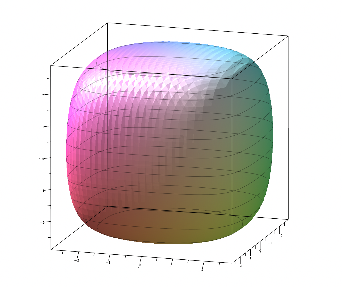
The boundary does not contain any zero or pole of and also does not contain any singular point of . Then defines an element in (see Theorem 1.11). Using Maple, one can describe the boundary of the Deninger chain in polar coordinates for as in Figure 1.
By Theorem 2.2, we have the following equality conditionally on Conjecture 2.1.6
where defined in (3.2.1) and the pairing is given by
Recall that is a singular surface with Picard rank 20 over (see Proposition 3.3). We have the following direct sum decomposition (see Proposition 2.4)
We then write as follows
| (3.3.1) |
where for . By using the following decomposition
one also has
| (3.3.2) |
where for . We then have
| (3.3.3) |
where the pairings are given by
Applying (2.2.24) to and , one get
Under Beilinson's conjecture 2.13 to and , one obtains that
| (3.3.4) |
where is the newform of weight 3 defined as follows. Recall that is isomorphic to the elliptic surface associated to (see the proof of Proposition 3.3). In particular, has a canonical fibration whose generic fiber is the elliptic curve (defined over )
By Remark 4.11, the singular fibers of are of types and . We then have
where is the number of simple components in the singular fiber (see [SI77, Lemma 1.3]). By Theorem 2.12, is the newform of weight 3 and level 7. In conclusion, we have
| (3.3.5) |
Remark 3.5.
In order to show that the coefficients in (3.3.5) are nonzero, one has to show that the decompositions (3.3.1) and (3.3.2) in terms of transcendental and algebraic parts are nontrivial decompositions. However, it seems that it is not trivial. One possible direction is using higher Chow groups to express the Mahler measure and see the actions of the projectors associated to the algebraic cycles on elements in higher Chow groups.
4. Appendix
4.1. Dualizing sheaves
This section is to recall the dualizing complex and dualizing sheaf of separated schemes of finite type over a field. It allows us to compute the dualizing sheaf of the compactification of the Maillot variety (see Section 3.1).
First let us recall some basic notions in derived categories. For a scheme , we denote by the category of -modules and the derived category associated to (see [Sta24, Tag 05RU]). Let be a morphism of schemes. The functor induces the right derived functor of derived categories
which is defined as follows. For every complex of -modules , there exists a -injective complex whose terms are injective -modules and a quasi-isomorphism which is termwise injective (see [Sta24, Tag 079P]). One defines and it does not depend on the choice of -injective complex (see [Sta24, Tag 079V]). Recall that the functor induces the derived pull back
| (4.1.1) |
which is as follows. For every complex of -modules , there exists -flat complex whose terms are flat -modules and a quasi-isomorphism which is termwise surjective (see [Sta24, Tag 06YF]). One defines and it does not depend on the choice of -flat complex (see [Sta24, Tag 06YI]).
Let denote the subcategory of complexes whose cohomology sheaves are quasi-coherent. We have If is a morphism between quasi-separated and quasi-compact schemes, then has a right adjoint (see [Sta24, Tag 0A9D])
whic maps to , where denotes the bounded below subcategory (see [Sta24, Tag 0A9I]). Recall that if be a morphism of separated schemes of finite type over a Noetherian scheme, the upper shriek functor
is defined as follows. Let be a compactification of over , i.e., a quasi-compact open immersion into a scheme proper over . This compactification exists (see Nagata's theorem [Sta24, Tag 0A9Z, Tag 0F41]). Denote by the right adjoint of . Notice that since is an embedding, is an exact functor. We then have . Then for , one defines the upper shriek functor by
which is an object in since maps to . This definition does not depend on the choice of compactifications (see [Sta24, Tag 0AA0]).
Definition 4.1 (Dualizing complex, Dualizing sheaf, [Sta24, Tag 0AWJ]).
Let be an equidimensional separated of finite type over a field . The dualizing complex of is defined by
The dualizing sheaf of is defined by
The following lemma says that if is a smooth proper scheme, the definition of dualizing sheaf above coincides with the definition of usual canonical sheaf.
Let us recall the notion of derived tensor product. Let be a scheme. Let be an object of and be a -flat complex (see (4.1.1) for the definition). We have a functor of the category of complexes of -modules
This functor induces a functor , denoted by . Let be a closed immersion. Consider the functor For a sheaf , the sheaf is a sheaf of -modules annihilated by the ideal sheaf . Since the functor is fully faithful with the image those -modules annihilated by (see [Sta24, Tag 08KS]), there exists an -module, denoted by , such that as -modules. It defines a functor
Recall that an effective Cartier divisor on a scheme can be seen as a closed subscheme whose ideal is an invertible -module. We have the following lemma, which is useful to compute the dualizing sheaf of the Maillot variety in Section 3.1.
Lemma 4.3.
Let be a Noetherian scheme and let be an effective Cartier divisor. Then the dualizing complex of is given by
Proof.
4.2. Elliptic surfaces
In this section, we recall some basic notion of elliptic surfaces. Let be a field such that . Let be a smooth projective curve over a field . An elliptic surface over is a smooth projective surface with a surjective morphism such that
-
(i)
is relatively minimal, i.e., for all , does not contain any curve satisfying that and .
-
(ii)
Let be the generic point of . The generic fiber is an elliptic curve over (i.e., and has a -rational point).
-
(iii)
There exists such that is singular.
4.2.1. Elliptic modular surfaces
Let be the upper half-plane. The action of on is given by
For an integer , one defines
A congruence subgroup of is a subgroup of containing for some integer . One considers the following congruence subgroups
Definition 4.5 (Modular curves).
The modular curve associated to a congruence subgroup is defined to be the Riemann surface , denoted by . The Riemann surface can be compactified by adding the finite set of points . One denotes by this compactification and the finite set of points added is called the set of cusps of .
Remark 4.6.
Let be a congruence subgroup of . The modular curves and are defined over some number field. Moreover, if for , then and are defined over (see [Shi94, Section 6.7]).
We set where acts on as follows
| (4.2.1) |
The space is a complex analytic manifold of dimension 2 and we have a holomorphic projection
such that for each , the fiber . We consider the following action of on
This action is not free, so it is necessary to consider congruence subgroup that acting freely on to form the quotient in the category of complex analytic varieties. For example, acts freely on if and only if .
Definition 4.7 (The universal elliptic curve).
Let be a congruence subgroup of acting freely on . The universal elliptic curve over is defined to be the quotient together with the canonical projection . It can be shown that the universal elliptic curve is an algebraic variety.
Definition 4.8 (The elliptic modular surfaces associated to ).
Let be a congruence subgroup of acting freely on . By [SS19, Theorem 5.19], there exists uniquely an elliptic surface associated to . We call it by the elliptic modular surface associated to .
Lemma 4.9.
Let be the elliptic modular surface associated to . We have
| (4.2.2) |
where is the complex vector space of cusp forms of weight and level .
Proof.
Denote by be the relative dualizing sheaf of (see Definition 4.4). As is a smooth projective surface and is a projective flat morphism, we have
| (4.2.3) |
where is the canonical sheaf of and is the canonical sheaf of . Denote by . From formula (4.2.3), we have
| (4.2.4) |
We recall the following natural isomorphism, which is called the Shimura isomorphism (see [Shi59])
| (4.2.5) |
for . This implies that and ∎
4.2.2. Elliptic surfaces
An elliptic surface is an elliptic surface where is an algebraic surface. The following result gives us conditions when an elliptic modular surface is an elliptic surface.
Proposition 4.10.
Let be a congruence subgroup of acting freely on the upper half-plane and let be the associated elliptic modular surface. Then is an elliptic surface if and only if
where is the complex vector space of cusp forms of weight , level .
Proof.
Suppose that is an elliptic surface. In particular, we have . Then by formula (4.2.2), we have As is an algebraic surface, by formula (4.2.2), we also have
Now we prove the converse. Again by formula (4.2.2), implies that Therefore, is a smooth projective curve of genus 0, hence . Let
where is the relative dualizing sheaf of (see Definition 4.4). By definition of elliptic surfaces, is not isotrivial, we can write for some suitable positive integer . The positivity of follows from the positivity of the direct image of the relative canonical sheaf. From the formula (4.2.3), we then have
By Shimura's isomorphism (4.2.5), we have
Therefore, . Hence . We consider Leray spectral sequence
which degenerates at -term (see e.g., [PS08, Section 1.3]). Since , one obtains that
and This implies that
As is a projective morphism and is normal, we have (see e.g., [Har77, proof of Corollary III.11.4]). Therefore, we have ∎
Example 4.11 (The elliptic modular surface associated to ).
Denote by . Recall that the modular curves and are algebraic curves defined over (see Remark 4.6). By Lemma 4.9, we have . Denoted by the function field of . We consider the following elliptic curve defined over
| (4.2.6) |
together with the point . This curve is an elliptic curve if and only if the discriminant
i.e., One can check that has exact order for . Denote by the open surface defined by the equation (4.2.6), together with the action (4.2.1). It can be shown that there is an isomorphism such that the canonical projection is the universal elliptic curve associated to . By [SS19, Theorem 5.19], one obtains an elliptic surface whose generic fiber is isomorphic to , and following commutative diagram
By Proposition 4.10 and the fact that and , is an algebraic surface defined over . The elliptic surface has 6 singular fibers corresponding to the 6 cusps . Let us compute the Kodaira type of these singular fibers. The Weierstrass equation (4.2.6) has coefficients At , the vanishing order of the discriminant is It follows from the [SS19, Table 5.1] that, these singular fibers are of type . At is a root of , the vanishing orders of the discriminant is hence the singular fibers at the roots of are of type . Therefore, the Picard rank is given by
where is the rank of the Mordell-Weil group . On the other hand, since is a surface, we have . This implies that and , hence is a singular surface. The Néron-Severi group has a -basis given by the divisor classes of
| (4.2.7) |
where is the closure of the trivial point of curve in , is a general fiber, and for are the irreducible components of the singular fiber (see [SS19, Proposition 6.3]). Recall that, for any point , its closure in gives rise to a curve isomorphic to , hence isomorphic to . It follows from the Weierstrass equation (4.2.6) that a general fiber is an elliptic curve defined over . The singular fiber is irreducible, hence does not contribute any generator to the basis (4.2.7) of . The singular fiber consists of 7 irreducible components, which are projective smooth rational curves, hence isomorphic to . Therefore, each singular fiber contributes 6 curves isomorphic to to the basis (4.2.7). This implies that is a singular surface with Picard rank over .
References
- [BCP97] Wieb Bosma, John Cannon and Catherine Playoust ``The Magma algebra system. I. The user language'' Computational algebra and number theory (London, 1993) In J. Symbolic Comput. 24.3-4, 1997, pp. 235–265 DOI: 10.1006/jsco.1996.0125
- [Bea96] Arnaud Beauville ``Complex algebraic surfaces.'' 34, Lond. Math. Soc. Stud. Texts Cambridge: Cambridge Univ. Press, 1996
- [Ber+15] Marie José Bertin et al. ``Classifications of elliptic fibrations of a singular K3 surface'' In Women in numbers Europe 2, Assoc. Women Math. Ser. Springer, Cham, 2015, pp. 17–49 DOI: 10.1007/978-3-319-17987-2\_2
- [Bor74] Armand Borel ``Stable real cohomology of arithmetic groups'' In Ann. Sci. École Norm. Sup. (4) 7, 1974, pp. 235–272
- [Boy06] David W. Boyd ``Conjectural explicit formulas for the Mahler measure of some three variable polynomials'' Unpublished notes, 2006
- [Bru20] François Brunault ``Unpublished list of conjectural identities for 3-variable Mahler measures'', 2020
- [Bru23] François Brunault ``On the Mahler measure of '' arXiv:2305.02992, 2023
- [Bur97] Jose Ignacio Burgos ``Arithmetic Chow rings and Deligne-Beilinson cohomology'' In J. Algebraic Geom. 6.2, 1997, pp. 335–377
- [BZ20] François Brunault and Wadim Zudilin ``Many variations of Mahler measures. A lasting symphony'' 28, Aust. Math. Soc. Lect. Ser. Cambridge: Cambridge University Press, 2020 DOI: 10.1017/9781108885553
- [Den97] Christopher Deninger ``Deligne periods of mixed motives, -theory and the entropy of certain -actions'' In J. Am. Math. Soc. 10.2, 1997, pp. 259–281 DOI: 10.1090/S0894-0347-97-00228-2
- [FSV00] Eric M. Friedlander, Andrei Suslin and Vladimir Voevodsky ``Introduction'' In Cycles, transfers, and motivic homology theories Princeton, NJ: Princeton University Press, 2000, pp. 3–9
- [Gon95] Alexander B. Goncharov ``Geometry of configurations, polylogarithms, and motivic cohomology'' In Adv. Math. 114.2, 1995, pp. 197–318 DOI: 10.1006/aima.1995.1045
- [Gon98] Alexander B. Goncharov ``Explicit regulator maps on polylogarithmic motivic complexes'' In Motives, polylogarithms and Hodge theory. Part I: Motives and polylogarithms. Papers from the International Press conference, Irvine, CA, USA, June 1998 Somerville, MA: International Press, 1998, pp. 245–276
- [GR22] Alexander B. Goncharov and Daniil Rudenko ``Motivic correlators, cluster varieties and Zagier’s conjecture on '' https://arxiv.org/pdf/1803.08585, 2022
- [Har77] Robin Hartshorne ``Algebraic geometry'' No. 52, Graduate Texts in Mathematics Springer-Verlag, New York-Heidelberg, 1977, pp. xvi+496
- [Huy16] Daniel Huybrechts ``Lectures on K3 surfaces'' 158, Cambridge Studies in Advanced Mathematics Cambridge University Press, Cambridge, 2016, pp. xi+485 DOI: 10.1017/CBO9781316594193
- [Jeu00] Rob Jeu ``Towards regulator formulae for the -theory of curves over number fields'' In Compos. Math. 124.2, 2000, pp. 137–194 DOI: 10.1023/A:1026440915009
- [Kah20] Bruno Kahn ``Zeta and -functions of varieties and motives'' Translated from the 2018 French original [3839285] 462, London Mathematical Society Lecture Note Series Cambridge University Press, Cambridge, 2020, pp. vii+207 DOI: 10.1017/9781108691536
- [KMP07] Bruno Kahn, Jacob P. Murre and Claudio Pedrini ``On the transcendental part of the motive of a surface'' In Algebraic cycles and motives. Volume 2. Selected papers of the EAGER conference, Leiden, Netherlands, August 30–September 3, 2004 on the occasion of the 75th birthday of Professor J. P. Murre Cambridge: Cambridge University Press, 2007, pp. 143–202
- [Lal15] Matilde Lalín ``Mahler measure and elliptic curve -functions at '' In J. Reine Angew. Math. 709, 2015, pp. 201–218 DOI: 10.1515/crelle-2013-0107
- [Lec23] Odile Lecacheux personal communication, 2023
- [Liv95] Ron Livné ``Motivic orthogonal two-dimensional representations of '' In Israel J. Math. 92.1-3, 1995, pp. 149–156 DOI: 10.1007/BF02762074
- [Mah62] Kurt Mahler ``On some inequalities for polynomials in several variables'' In J. London Math. Soc. 37, 1962, pp. 341–344 DOI: 10.1112/jlms/s1-37.1.341
- [Mai03] Vincent Maillot ``Mahler measure in Arakelov geometry'' Workshop lecture at ``The many aspects of Mahler's measure'', Banff International Research Station, 2003
- [Nek94] Jan Nekovář ``Beĭlinson's conjectures'' In Motives (Seattle, WA, 1991) 55, Part 1, Proc. Sympos. Pure Math. Amer. Math. Soc., Providence, RI, 1994, pp. 537–570 DOI: 10.1090/pspum/055.1/1265544
- [PS08] Chris A.. Peters and Joseph H.. Steenbrink ``Mixed Hodge structures'' 52, Ergeb. Math. Grenzgeb., 3. Folge Berlin: Springer, 2008 DOI: 10.1007/978-3-540-77017-6
- [Sch10] Matthias Schütt `` surfaces with Picard rank 20'' In Algebra Number Theory 4.3, 2010, pp. 335–356 DOI: 10.2140/ant.2010.4.335
- [Sch94] A.. Scholl ``Classical motives'' In Motives (Seattle, WA, 1991) 55, Part 1, Proc. Sympos. Pure Math. Amer. Math. Soc., Providence, RI, 1994, pp. 163–187 DOI: 10.1090/pspum/055.1/1265529
- [Shi59] Goro Shimura ``On integrals attached to automorphic forms'' In J. Math. Soc. Japan 11, 1959, pp. 291–311 DOI: 10.2969/jmsj/01140291
- [Shi94] Goro Shimura ``Introduction to the arithmetic theory of automorphic functions.'' 11, Publ. Math. Soc. Japan Princeton, NJ: Princeton Univ. Press, 1994
- [SI77] Tetsuji Shioda and Hiroshi Inose ``On singular K3 surfaces'', Complex Anal. algebr. Geom., Collect. Pap. dedic. K. Kodaira, 119-136 (1977)., 1977
- [SS19] Matthias Schütt and Tetsuji Shioda ``Mordell-Weil lattices'' 70, Ergeb. Math. Grenzgeb., 3. Folge Singapore: Springer, 2019
- [Sta24] Projects Stack ``The Stacks project authors'', 2024 URL: https://stacks.math.columbia.edu
- [Sus90] Andrei Suslin `` of a field, and the Bloch group'' Translated in Proc. Steklov Inst. Math. 1991, no. 4, 217–239, Galois theory, rings, algebraic groups and their applications (Russian) In Trudy Mat. Inst. Steklov. 183, 1990, pp. 180–199\bibrangessep229
- [Tri23] Thu Ha Trieu ``The Mahler measure of exact polynomials in three variables'' submitted, available on arxiv:2310.06563v4, 2023, pp. 40 pages
- [Tri24] Thu Ha Trieu ``Doctoral thesis'' available here, 2024
- [Zag91] Don Zagier ``Polylogarithms, Dedekind zeta functions, and the algebraic K-theory of fields'', Arithmetic algebraic geometry, Proc. Conf., Texel/Neth. 1989, Prog. Math. 89, 391-430 (1991)., 1991