Wedge Holographic Complexity in Karch-Randall Braneworld

Abstract

We investigate holographic complexities in the context of wedge holography, focusing specifically on black string geometry in AdS₃. The wedge spacetime is bounded by two end-of-the-world (EOW) branes with intrinsic Dvali-Gabadadze-Porrati (DGP) gravity. In line with this codimension-two holography, there are three equivalent perspectives: bulk perspective, brane perspective, and boundary perspective. Using both the “Complexity=Volume” (CV) and “Complexity=Action” (CA) proposals, we analyze the complexity in wedge black string geometry in the tensionless limit. By treating the branes as rigid, we find the late-time growth rates of CV and CA match exactly across bulk and brane perspectives. These results are consistent with those from JT gravity, with additional contributions from the intrinsic gravity of the branes. For fluctuating branes, we find that the late-time growth rates of CV and CA match between bulk and brane perspectives at the linear order of fluctuation. The CV results exhibit $\frac{\phi_{h}^{2}}{\phi_{0}}$ corrections from fluctuations, consistent with the findings in previous work. Moreover, the CA results reveal an additional constant term in the fluctuating branes case. We provide an interpretation of this in terms of gravitational edge mode effects. The distinct corrections arising from fluctuations in the CA and CV proposals suggest that the CV proposal is more sensitive to geometric details. Furthermore, we discuss these results in relation to Lloyd’s bound on complexity, their general time dependence, and the effects of fluctuations.

1 Introduction

AdS/CFT correspondence Maldacena:1997re ; Gubser:1998bc ; Witten:1998qj offers a powerful framework for understanding quantum gravity, one of the most important challenges in modern theoretical physics. It connects observables in $d$-dimensional bulk spacetime to those in codimension-one boundary field theory. Later developments proposed a holographic duality between bulk gravity and boundary CFTs, now known as AdS_d/BCFT_d-1 Takayanagi:2011zk ; Fujita:2011fp ; Karch:2000gx . This form of holography is naturally realized in the Karch-Randall braneworld Randall:1999ee ; Randall:1999vf ; Gubser:1999vj ; Karch:2000ct , where an end-of-the-world (EOW) brane is present in the bulk spacetime described by (semi)classical gravity, see Yadav:2023qfg ; Wen:2024uwr ; Lin:2023ajt ; Aguilar-Gutierrez:2023tic ; Aguilar-Gutierrez:2023ccv ; Aguilar-Gutierrez:2023zoi ; Kim:2023adq ; Chang:2023gkt ; Yadav:2023sdg ; Li:2023fly ; Kanda:2023zse ; Miao:2023unv ; Hu:2022zgy for recent work on entanglement and complexity in this background. Furthermore, an additional EOW brane can be introduced in the bulk, intersecting with the first at the asymptotic boundary, forming a wedge near the boundary. This codimension-two holography is referred to as wedge holography Akal:2020wfl ; Geng:2020qvw ; Bousso:2020kmy ; Miao:2020oey , which posits a holographic duality between a wedge gravitational theory and a codimension-two CFT located at the corner of the wedge. Recent work has demonstrated that in the AdS₃ wedge spacetime, with two fluctuating branes, the gravitational action reduced to JT gravity in the brane tensionless limit Geng:2022tfc ; Geng:2022slq .

On the other hand, studying the black hole interior quantum mechanically is always crucial and compelling, particularly in the context of the black hole information paradox. While the AMPS Almheiri:2012rt proposal introduced the idea of a firewall, an alternative resolution was offered by Maldacena and Susskind through the ER=EPR conjecture Maldacena:2013xja , which states that two entangled states are connected by an Einstein-Rosen (ER) bridge. To analyze the entanglement of these states, one can compute the entanglement entropy holographically using the Ryu-Takayanagi (RT) formula Ryu:2006bv . However, it was later suggested that entanglement entropy alone is insufficient to describe the late-time growth of the ER bridge after the rapid thermalization of the black hole. This observation has led to the exploration of the computational complexity of states, or its dual, holographic complexity Susskind:2014moa .

In the spirit of bulk/boundary correspondence, the computational complexity of states in the boundary field theory is dual to the holographic complexity in bulk gravity. In the context of two-sided black holes, the holographic complexity is proposed to be equivalent to the length or volume of an extremal codimension-one hypersurface connecting the boundary states, known as the “Complexity=Volume” (CV) proposal Susskind:2014rva ; Stanford:2014jda . Later, an alternative proposal-known as the “Complexity=Action” (CA) proposal Brown:2015bva -suggested that the complexity of boundary states is dual to the on-shell gravitational action within a bounded “Wheeler-DeWitt” (WDW) patch in the bulk. Due to the nature of asymptotic AdS spacetime, it is necessary to consider a regularized WDW patch to avoid the coordinate divergence that arises near the boundary.

A universal feature of holographic complexity is its linear growth at late times. The rate of this growth (or slope) is shown to be constrained by Lloyd’s bound in the AdS-Schwarzchild black hole Brown:2015lvg ; Engelhardt:2021mju . Lloyd’s bound is proportional to the energy of the boundary states, which corresponds to the mass of the black hole. However, it has been observed that, for certain periods, the growth rate can exceed this bound, violating Lloyd’s bound at specific times Aguilar-Gutierrez:2023ccv .

One of the interesting problems is the exploration of differences between CV and CA proposals, as this may lead to a more precise definition of holographic complexity and its relation to boundary complexities Iliesiu:2021ari ; Yang:2020tna . For instance, the regularized wormhole length has been proposed as dual to the Krylov state complexity at the boundary Rabinovici:2023yex . To better understand this relationship, it is crucial to test CV and CA proposals in various geometric settings, particularly those with non-trivial boundaries. Notably, CV and CA are found to have different divergent behaviors in the presence of a single boundary Chapman:2018bqj ; Braccia:2019xxi .

This paper aims to investigate the late-time growth rates of CV and CA in AdS₃ wedge holography, with two timelike AdS₂ EOW branes that can be either rigid or fluctuating. In the spirit of wedge holography, holographic complexity can be read from both bulk and brane perspectives. To be more general, we will also consider contributions from intrinsic gravity residing on the branes.

This paper is organized as follows: In the next section, we will review the general setup of wedge holography, including the effective action on two EOW branes, the emergence of JT gravity in AdS₃, and proposals of CV and CA for wedge holographic complexity. In sections 3 and 4, we will analyze CV and CA proposals for both rigid and fluctuating branes from the perspectives of the bulk and brane. Section 5 will focus on Lloyd’s bound and its relation with late-time growth rates of wedge holographic complexities, the general time-dependence of CV and CA, and the effects of fluctuations on these results. Finally, we will summarize our main results and discuss possible directions for future research.

2 Review of previous work

2.1 Wedge holography

This section reviews the basic setups and concepts of wedge holography and its geometry background. We will mainly focus on AdS₃ wedge holography, where the bulk is asymptotic AdS₃ (semi-)classical Einstein gravity with two asymptotic AdS₂ EOW branes denoted as $Q_{1}$ and $Q_{2}$:

$$S_{\text{AdS}_{3}}=-\frac{1}{16\pi G_{3}}\int d^{3}x\sqrt{-g_{3}}\left[R_{\text{bulk}}+\frac{2}{l^{2}_{3}}\right]-\frac{1}{8\pi G_{3}}\int_{Q_{1}+Q_{2}}d^{2}x\sqrt{-h}(K-T),$$ (1)

where $R_{\text{bulk}}$ is the AdS₃ bulk Ricci scalar, $h$ is the induced metric on the EOW brane, $K$ and $T$ respectively denote the trace of extrinsic curvatures and tensions for branes $Q_{1}$ and $Q_{2}$. They shall satisfy the Neumann boundary condition consistent with the foliation geometry Israel:1966rt ; Misner:1973prb ; Takayanagi:2011zk ; Fujita:2011fp :

$$K_{ab}=(K-T)h_{ab}.$$ (2)

The equation of motion of this action admits AdS₂ foliation geometries of AdS₃:

$$ds^{2}=dy^{2}+\cosh^{2}\left(\frac{y}{l_{d}}\right)ds^{2}_{\text{AdS}}.$$ (3)

This geometry well pictures the wedge holography as shown in figure 1. We focus particularly on the black string foliation geometry, as it is related to the later discussions on holographic complexity, especially regarding its late-time growth rates. Our discussion will be based on three-dimensional asymptotic AdS spacetime, leading to a geometry background characterized by an AdS₃ black string with AdS₂ foliations:

$$ds^{2}=dy^{2}+\cosh^{2}\left(\frac{y}{l_{3}}\right)\left(-\frac{r^{2}-r_{h}^{2}}{l_{3}^{2}}dt^{2}+\frac{l_{3}^{2}}{r^{2}-r_{h}^{2}}dr^{2}\right).$$ (4)

It is also noteworthy that the AdS₃ black string geometry can be obtained through coordinates transformations from AdS₃ global patch (see appendix A).

Figure 1: The left figure is a sketch of wedge holography at a constant time slice. Here we show a plot with compactified $y$ coordinate, which is equivalent to the uncompactified case Akal:2020wfl . $Q_{1}$ and $Q_{2}$ are two EOW branes with positions at $y_{1}$ and $y_{2}$. The blue dots are defects at the asymptotic boundaries. $r_{max}$ is the UV cut-off. The right figure is an AdS_d-1 slice, where the blue lines are asymptotic boundaries at which the defects are located.

In this wedge spacetime, it is proposed to be a codimension two holographic system Akal:2020wfl ; Geng:2020qvw ; Bousso:2020kmy ; Miao:2020oey , which can be understood from three equivalent perspectives:

Bulk perspective: Classical Einstein-Hilbert gravity.

Brane perspective: Two codimension-one CFTs live on the branes, minimally coupled with intrinsic Dvali-Gabadadze-Porrati (DGP) gravity on the branes. The two branes are connected via defects located at the asymptotic boundaries.

Boundary perspective: A codimension-two CFT lives at the shared asymptotic boundary of branes.

Consequently, the complexity of boundary codimension-two CFT has not only just one, but two holographic correspondences. Later, we will primarily focus on CV and CA proposals from bulk and brane perspectives and examine their equivalence in terms of holographic complexity.

2.2 Tensionless limit and emergent JT gravity

In Geng:2022slq ; Geng:2022tfc , it is shown that an emergent JT gravity action arises from wedge holography in the Karch-Randall braneworld with two fluctuating branes in the tensionless limit. Let us start with an AdS₃ gravitational action with two boundaries as two Karch-Randall branes. The action takes the form

$$S_{\text{AdS}_{3}} = -\frac{1}{16\pi G_{3}}\int dyd^{2}x\sqrt{-g_{3}}\left[R_{\text{bulk}}+\frac{2}{l_{3}^{2}}\right]-\frac{1}{8\pi G_{3}}\int_{Q_{1}}d^{2}x\sqrt{-h_{1}}(K_{1}-T_{1})$$ (5)

$$-\frac{1}{8\pi G_{3}}\int_{Q_{2}}d^{2}x\sqrt{-h_{2}}(K_{2}-T_{2}).$$

Here, instead of two rigid branes, we consider two fluctuating branes with locations set as $y=y_{1}+\delta\phi_{1}(r)<0$ and $y=y_{2}+\delta\phi_{2}(r)>0$, where $r$ denotes the radial coordinate living on the brane. By solving the Israel junction condition, we can find the branes tensions are

$$T_{1}=\tanh\frac{\left|y_{1}\right|}{l_{3}},\ \ \ T_{2}=\tanh\frac{y_{2}}{l_{3}},$$ (6)

which are half of the trace of extrinsic curvatures without brane fluctuations. This action admits the foliation geometry as a solution in AdS₃ black string as we showed in section 2.1:

$$ds^{2}=dy^{2}+\cosh^{2}\left(\frac{y}{l_{3}}\right)g_{2ab}(x)dx^{a}dx^{b},$$ (7)

where $x^{a}=(t,r)$ are the coordinates on the brane, and assume that $\delta\phi_{1}(r),\delta\phi_{2}(r)\ll l_{3}$, and the induced metric on the brane is $g_{2ab}(y,x)\approx g_{2ab}(x)$ if we only consider lowest graviton mode (low energy limit). We set $g_{\mu y}=0$ and $g_{yy}=1$ after fixing the bulk diffeomorphism. We thus have

$$\sqrt{-g_{3}}=\cosh\left(\frac{y}{l_{3}}\right)\sqrt{-g_{2}}.$$ (8)

Given the bulk geometry (7), we can write down the bulk Ricci scalar as:

$$R_{\rm{bulk}}=\frac{1}{\cosh^{2}(y/l_{3})}R_{\text{brane}}(x)-\frac{4+2\tanh^{2}(y/l_{3})}{l^{2}_{3}}.$$ (9)

From now on, we will keep the brane tensions fixed and extrinsic curvatures that depend on the brane’s internal fluctuating. If we only keep linear terms of $\delta\phi_{1}(r)$ and $\delta\phi_{2}(r)$, we can then find out the extrinsic curvatures as:

$$K_{1}=2\tanh\left(\frac{-y_{1}-\delta\phi_{1}(r)}{l_{3}}\right),\ \ \ K_{2}=2\tanh\left(\frac{y_{2}+\delta\phi_{2}(r)}{l_{3}}\right).$$ (10)

We can thus plug (9) and (10) into the bulk action (5). The effective gravitational integral turns out to be

$$S_{\text{eff}}=-\frac{1}{16\pi G_{3}}\int^{y_{2}+\delta\phi_{2}(r)}_{y_{1}+\delta\phi_{1}(r)}dy\int dtdr\sqrt{-g_{2}}\cosh^{2}\left(\frac{y}{l_{3}}\right)\left[\frac{R_{\text{brane}}(x)}{\cosh^{2}(y/l_{3})}-\frac{2+2\tanh^{2}(y/l_{3})}{l^{2}_{3}}\right].$$

We can then denote $y_{2}-y_{1}=\phi_{0}$ and $\delta\phi_{2}(r)-\delta\phi_{1}(r)=\phi(r)$, where $\phi_{0}$ is the constant dilaton and $\phi(r)$ is the radion in the context of Randall-Sundrum Braneworld I Randall:1999ee (it is identified as the dynamical dilaton field in two dimensions). We are able to rewrite the effective action as:

$$S_{\rm{eff}}=-\frac{\phi_{0}}{16\pi G_{3}}\int d^{2}x\sqrt{-g_{2}}R\left[g_{2}\right]-\frac{1}{16\pi G_{3}}\int d^{2}x\sqrt{-g_{2}}\phi(x)\left(R\left[g_{2}\right]+\frac{2}{l_{3}^{2}}\right),$$ (12)

which is the pure JT gravity action, where the first term is the topological term and the second term is the linear dilaton potential term. There will also be dilaton dynamical terms that are irrelevant to our discussion.

Notably, our review of emergent JT gravity above and calculations later depend on the small fluctuation (tensionless limit). It is thus important to discuss the validity of dilaton profiles in our calculations. In the metric we choose (4), the time-independent dynamical dilaton profile is the solution of the equation of motion, which is written as

$$\phi(r)=\frac{\phi_{h}}{r_{h}}r.$$ (13)

At the cut-off boundary $r_{max}$ shown in the figure 1, the dilaton profile behaves as $\phi_{b}\sim\frac{\phi_{h}}{r_{h}}r_{max}$ or $\phi_{b}\sim\frac{\phi_{h}}{r_{h}\epsilon}$ . As approaching the asymptotic boundary $r_{max}\rightarrow\infty$ or $\epsilon\rightarrow 0$, our calculation is valid only when $\frac{\phi_{h}}{l_{3}}$ approaching to zero faster than $\epsilon$, namely, it is of order $O(\frac{1}{r^{2}_{max}})$ or $O(\epsilon^{2})$ Geng:2022slq ; Geng:2022tfc . Practically, in our calculations, we consider $\phi_{h}\ll\phi_{0}\ll l_{3}$ and $\phi(r_{max})\ll\phi_{0}$ which, in the high-dimensional Reissner–Nordström black hole, are understood as the near extremal limit Maldacena:2016upp .

2.3 Brane effective action

In our setup, we can further consider two EOW branes with intrinsic DGP gravity. Let us only consider the case where the bulk is asymptotically AdS₃ and branes are asymptotically AdS₂ Chen:2020uac . The intrinsic brane action is written as:

$$S_{\text{brane}}=\frac{1}{16\pi G_{\text{brane}}}\int d^{2}x\sqrt{-g_{2}}R_{\text{brane}},$$ (14)

where the metric $g_{2}$ is the induced metric on the brane and $R_{\text{brane}}$ is the intrinsic curvature scalar only involving induced metric $g_{2}$. Adding this Einstein-Hilbert term in two dimensions does not change the position of the brane Chen:2020uac , namely the Israel junction condition.

The total effective action on the branes should be given as

$$S^{Q}_{\text{eff}}=S^{Q_{1}}_{\text{induced}}+S^{Q_{2}}_{\text{induced}}+S^{Q_{1}}_{\text{brane}}+S^{Q_{2}}_{\text{brane}},$$ (15)

where the induced action is

$$S^{Q}_{\text{induced}}=S^{Q_{1}}_{\text{induced}}+S^{Q_{2}}_{\text{induced}}=S^{Q}_{\text{gravity}}+S^{Q}_{\text{CFT}},$$ (16)

and $S^{Q}_{\text{CFT}}=-\frac{1}{8\pi G_{3}}\int_{Q_{1}}d^{2}x\sqrt{-g_{2}}T^{Q_{1}}_{\text{brane}}-\frac{1}{8\pi G_{3}}\int_{Q_{2}}d^{2}x\sqrt{-g_{2}}T^{Q_{2}}_{\text{brane}}$, where $T_{\text{brane}}$ is the brane tension that will be specified later, and $S^{Q}_{\text{gravity}}=-\frac{1}{16\pi G_{3}}\int^{y_{2}}_{y_{1}}dy\int d^{2}x\sqrt{-g_{3}}\left[R_{\text{bulk}}+\frac{2}{l^{2}_{3}}\right]-\frac{1}{8\pi G_{3}}\int_{Q_{1}+Q_{2}}d^{2}x\sqrt{-h}K$ is the action induced on the brane by the bulk gravity. To find the induced gravitational action Chen:2020uac ; Geng:2023iqd ; Myers:2024zhb on two branes (we consider branes in a symmetric position, namely, $y_{2}=-y_{1}=y_{b}$), one needs to integrate the bulk action with Gibbons-Hawking-York (GHY) terms over the radial direction (in our case, it is $y$-direction). In the wedge holography setup, two branes play the role of regulator surfaces so that no counter terms are needed. A convenient way of doing so is to consider the Fefferman-Graham expansion of the bulk metric near the brane Fefferman:1985 ; Fefferman:2007rka . Consequently, the boundary action after integration would only involve terms related to the intrinsic curvature of the boundary metric. The total induced action on two branes can be written as a dilaton $\Phi$ gravity action Chen:2020uac ; Myers:2024zhb

$$S^{Q}_{\text{induced}}=\frac{l_{3}}{16\pi G_{3}}\int d^{2}x\sqrt{-g_{2}}(f(\Phi)+f^{\prime}(\Phi)(R_{\text{brane}}-\Phi))+\frac{l_{3}}{8\pi G_{3}}\int dx\sqrt{-\gamma}Kf^{\prime}(\Phi),$$

where

$$f(\Phi)=\Phi\log\left(\frac{\sqrt{4+2\Phi l^{2}_{3}}+2}{\sqrt{4+2\Phi l^{2}_{3}}-2}\right)+\frac{1}{T_{\text{brane}}l_{3}}\left(\Phi+\frac{2}{l^{2}_{\text{brane}}}\right)+\sum_{n>1}c_{n}\left(\Phi+\frac{2}{l^{2}_{\text{brane}}}\right)^{n}.$$ (18)

The on-shell condition from this induced action is easy to find as

$$\Phi=R_{\text{brane}}=-\frac{2}{l^{2}_{\text{brane}}}=-\frac{2}{l_{3}^{2}}+2T^{2}_{\text{brane}}.$$ (19)

After applying the on-shell condition for dilaton $\Phi$, the induced action on the branes can be written as an effective $f(R)$ gravity:

$$S^{Q}_{\text{induced}}=\frac{l_{3}}{16\pi G_{3}}\int d^{2}x\sqrt{-g_{2}}f(R),$$ (20)

where

$$f(R)=R\log\left(\frac{\sqrt{4+2Rl^{2}_{3}}+2}{\sqrt{4+2Rl^{2}_{3}}-2}\right)+\frac{1}{T_{\text{brane}}l_{3}}\left(R+\frac{2}{l^{2}_{\text{brane}}}\right)+\sum_{n>1}c_{n}\left(R+\frac{2}{l^{2}_{\text{brane}}}\right)^{n}.$$ (21)

After imposing the on-shell condition for the curvature scalar, the action becomes

$$S^{Q}_{\text{induced}}=\frac{l_{3}}{16\pi G_{3}}\int_{Q}\sqrt{-g_{2}}\log\left(\frac{1+l_{3}T_{\text{brane}}}{1-l_{3}T_{\text{brane}}}\right)R_{\text{brane}}d^{2}x.$$ (22)

Further adding the brane intrinsic DGP terms, we find that the total action on the branes can be written as an effective Einstein-Hilbert action (we set AdS₃ length $l_{3}=1$ from now on)

$$S^{Q}_{\text{eff}}=\frac{1}{16\pi G_{\text{eff}}}\int_{Q}\sqrt{-g_{2}}R_{\text{brane}}d^{2}x,$$ (23)

where the effective Newton constant on the brane is

$$\frac{1}{G_{\text{eff}}}=\frac{1}{G_{3}}\log\left(\frac{1+T_{\text{brane}}}{1-T_{\text{brane}}}\right)+\frac{2}{G_{\text{brane}}},$$ (24)

and the Ricci scalar on the brane is

$$R_{\text{brane}}=-2(1-T^{2}_{\text{brane}}).$$ (25)

2.4 Wedge holographic complexities

The holographic duality in wedge spacetime is particularly intriguing due to the presence of double duals. This feature offers new perspectives when studying holographic complexity in the context of wedge holography.

In the traditional AdS/(B)CFT framework, holographic complexity is defined as the scalar quantity in the bulk that corresponds to codimension-one state complexity in the boundary. However, in wedge holography, the conformal boundary of bulk space forms a codimension-two defect on the boundary CFT. Therefore, we must consider the codimension-two boundary state complexity, which corresponds not only to bulk scalar quantities but also to scalar quantities on the two branes.

For the CV proposal, the conventional definition is the extremized codimension-one hypersurface anchored to the boundary states:

$$CV_{B}=\text{max}\left[\frac{V_{\text{bulk}}}{G_{N}l_{N}}\right],$$ (26)

where $V_{\text{bulk}}$ means the volume of the codimension-one hypersurface from the bulk perspective. However, in our setup with an intrinsic DGP term on the brane, inspired by Chen:2020uac ; Hernandez:2020nem in which in order to count the holographic entanglement entropy one needs to modify the RT formula to include an additional contribution caused by the DGP term on the brane, the state complexity at the boundary shall receive contributions from two branes in a similar manner. We need to add extremized volume on the branes bounded by the bulk extremal points:

$$CV_{Q}=\text{max}\left[\frac{V_{\text{brane}}}{G_{\text{brane}}l_{\text{brane}}}\right],$$ (27)

where $V_{\text{brane}}$ is the volume of the codimension-two hypersurface on the brane anchored to the same boundary states.

Since the induced action on two branes can be written effectively as an Einstein-Hilbert action with an effective Newton constant (see section 2.3), the CV proposal can also be written from the brane perspective:

$$\widetilde{CV}_{Q}=\text{max}\left[\frac{V_{\text{brane}}}{G_{\text{eff}}l_{\text{brane}}}\right].$$ (28)

Therefore, the CV proposal with our setup in wedge holography is

$$\boxed{CV_{\text{Wedge}}=CV_{B}+2CV_{Q}=\widetilde{CV}_{Q}.}$$ (29)

For the CA proposal, we need to evaluate four parts: bulk, boundary, joint, and brane contributions from the bulk perspective. The bulk term is given as

$$A_{\text{bulk}}=\frac{1}{16\pi G_{3}}\int_{\text{WDW}}d^{3}x\sqrt{-g}(R-2\Lambda),$$ (30)

where this term is the bulk on-shell Einstein-Hilbert action evaluated in the WDW patch. The boundary terms are written as

$$A_{\text{bdy}}=\frac{\epsilon_{K}}{8\pi G_{3}}\int_{\mbox{${\cal B}$}_{s}}d^{2}x\sqrt{|h|}K+\frac{\epsilon_{\kappa}}{8\pi G_{3}}\int_{\mbox{${\cal B}$}_{n}}d\lambda d\theta\sqrt{\gamma}\kappa+\frac{\epsilon_{\Theta}}{8\pi G_{3}}\int_{\mbox{${\cal B}$}_{n}}d\lambda dy\sqrt{\gamma}\Theta\log{(|\Theta|)},$$ (31)

where the first term is the boundary GHY term for the spacelike surfaces, $h$ is the induced metric on the boundary surface and $K$ is the trace of the extrinsic curvature of the boundary. For the spacelike boundary, $\epsilon_{K}=+1(-1)$ if the normal vector points into (out of) the WDW patch. The second term is the null boundary term, where $\lambda$ is the affine parameter and $\theta$ is the coordinate that is constant on each generator of the null hypersurface. $\kappa$ is the surface gravity defined to satisfy the geodesic equation: $k^{\mu}\nabla_{\mu}k^{\nu}=\kappa k^{\nu}$, where $k^{\mu}=\frac{dx^{\mu}}{d\lambda}$ is the future-directed null normal vector. And $\epsilon_{\kappa}=+1(-1)$ according to the WDW patch lying in the future (past) of the null boundary. The third term is the counter term, which is introduced to remove the parametrization dependence of the null generators. $\Theta=\partial_{\lambda}\log\gamma$, where $\gamma$ is the determinant of the metric on the null hypersurface. $\epsilon_{\theta}=+1(-1)$ if the WDW lying in the future (past) of the null hypersurface.

The joint terms that will be considered in this paper are given as

$$A_{\text{joint}}=\frac{\epsilon_{a}}{8\pi G_{3}}\int_{J_{n}}dx\sqrt{\gamma}a+\frac{\epsilon_{\eta}}{8\pi G_{3}}\int_{J_{ts}}dx\sqrt{|\sigma|}\eta,$$ (32)

where the first term is the null boundary involved joint, $a=\log|k\cdot s|$ for null and timelike joints, $a=\log|k\cdot n|$ for null and spacelike joints, and $a=\log|k\cdot k^{\prime}/2|$ for null and null joints, where $k$ and $k^{\prime}$ are null vectors tangent to the null boundary, $s$ is the unit normal vector to the timelike surface, and $n$ is the unit normal vector to the spacelike surface. The sign $\epsilon_{a}=+1$ if the WDW patch lies at the future (past) of the null boundary and the past (future) of the joint. For all other cases, $\epsilon_{a}=-1$. The second term is the joint of timelike and spacelike hypersurfaces, where $\sigma$ is the determinant of the metric living on the joint. $\eta=\log|n+p|\cdot s$, where $s$ is the unit normal vector to the timelike surface, which points outside of the WDW patch; $n$ is the unit normal vector to the spacelike surface, which points to the future direction; $p$ is the unit spatial vector on the spacelike surface and orthogonal to the joint. The sign $\epsilon_{\eta}=+1$ if $n$ points outside of the WDW patch. Otherwise, $\epsilon_{\eta}=-1$.

The brane terms are given as

$$A_{\text{brane}}=\frac{1}{8\pi G_{3}}\int_{Q\cap\text{WDW}}d^{2}x\sqrt{-h}(K-T)+\frac{1}{16\pi G_{\text{brane}}}\int_{Q\cap\text{WDW}}d^{2}x\sqrt{-g_{2}}R_{\text{brane}},$$ (33)

where we considered brane action from bulk gravity, the CFTs living on the branes, and intrinsic DGP terms. Therefore, from the bulk perspective, the total on-shell action constrained by the WDW patch in the CA proposal is

$$A_{B}=A_{\text{bulk}}+A_{\text{bdy}}+A_{\text{joint}}+A_{\text{brane}},$$ (34)

where $A_{B}$ denotes the action from the bulk perspective.

However, due to the nature of wedge holography, the defects at both boundaries are holographically dual to the bulk AdS₃ spacetime and two AdS₂ branes. Therefore, from the brane perspective, as discussed in section 2.3, the intrinsic action on the brane $Q_{1}$ and $Q_{2}$ shall be taken into account as well as the boundaries, joints, and counter terms on the branes:

$$\tilde{A}_{Q}=\tilde{A}_{\text{eff}}+\tilde{A}_{\text{bdy}}+\tilde{A}_{\text{joint}},$$ (35)

where the first term is the effective action on the two-dimensional brane (23), the other three terms are also on the brane but follow the same rules discussed in the bulk perspective. Here, we denote $\tilde{A}_{Q}$ as the action evaluated in the WDW patch from the brane perspective.

Therefore, given what we defined above and inspired by Akal:2020wfl , the CA proposal in our setup for wedge holography is

$$\boxed{A_{\text{Wedge}}=A_{\text{B}}=\tilde{A}_{\text{Q}}.}$$ (36)

In the next two sections, we will test the late-time growth rates of CV (29) and CA (36) proposals in AdS₃ wedge spacetime with AdS₂ branes in the tensionless limit. When branes are rigid, we find these proposals are exactly valid. When branes fluctuate, they remain valid in the leading order of fluctuation.

3 Complexity=Volume

In this section, we test the CV proposal (29) in AdS₃ black string geometry. While similar calculations were done solely from the bulk perspective Bhattacharya:2023drv , in this paper, we consider an additional contribution from brane’s intrinsic gravity and we will show the matching results from both bulk and brane perspectives for rigid and fluctuating branes within the framework of wedge holography. As reviewed in section 2.2, the results from the CV proposal shall agree with those from JT gravity, as shown in Bhattacharya:2023drv . Here, we focus specifically on the late-time growth rate of complexity, leaving the discussion of its saturation value, its relation to Lloyd’s bound, and its general time dependence in section 5.

3.1 Rigid branes

3.1.1 Bulk perspective

In AdS₃ wedge holography, we consider the bulk black string metric:

$$ds^{2}=dy^{2}+\cosh^{2}y\left(-(r^{2}-r_{h}^{2})dt^{2}+\frac{1}{r^{2}-r_{h}^{2}}dr^{2}\right),$$ (37)

where the AdS₃ length is 1. Since we consider symmetrically located branes, the induced metrics on two branes share the following metric:

$$ds^{2}_{Q_{1}/Q_{2}}=\cosh^{2}y_{b}\left(-(r^{2}-r_{h}^{2})dt^{2}+\frac{1}{r^{2}-r_{h}^{2}}dr^{2}\right),$$ (38)

where the AdS₂ length on each brane is $\cosh y_{b}$.

Consider the volume in the bulk enclosed by two rigid branes, which is anchored by boundary states at $t_{b}$ and $-t_{b}$:

$$V = \int_{-y_{b}}^{y_{b}}dy\int dr\cosh y\sqrt{-f(r)t^{\prime 2}+\frac{1}{f(r)}}$$ (39)

$$\approx 2y_{b}\int dr\sqrt{-f(r)t^{\prime 2}+\frac{1}{f(r)}},$$

where we take the tensionless limit in the second line. To extremize this volume functional, we defined the Lagrangian as:

$$L_{B}=\sqrt{-f(r)t^{\prime 2}+\frac{1}{f(r)}}.$$ (40)

Since the Lagrangian does not explicitly depend on $t$, there would be a conserved quantity along the whole hypersurface given as:

$$P_{B}=-\frac{\partial L}{\partial t^{\prime}(r)}=-\frac{t^{\prime}f(r)}{\sqrt{-f(r)t^{\prime 2}+\frac{1}{f(r)}}}.$$ (41)

We can solve this to find

$$t^{\prime}(r)=\frac{P_{B}}{f(r)\sqrt{P_{B}^{2}+f(r)}}.$$ (42)

The boundary time can be expressed as the integral of the above solution from the bulk turning point (extremal point) $r_{t}$ of the volume functional to the UV cutoff $r_{max}$:

$$t_{b}=\int^{r_{max}}_{r_{t}}dr\frac{P_{B}}{f(r)\sqrt{P_{B}^{2}+f(r)}}.$$ (43)

At this turning point, the time derivative of $r$ should vanish $1/t^{\prime}(r_{t})=0$, which gives us

$$P_{B}=\sqrt{r_{h}^{2}-r_{t}^{2}}.$$ (44)

For late times $t_{b}\rightarrow\infty$, the conserved quantity $P_{B}$ reaches a critical value $P_{B}^{c}(\infty)$ which is independent of $r_{t}$. Therefore, by setting $\frac{\partial P_{B}}{\partial r_{t}}=0$, we find the critical value of the conserved quantity:

$$P_{B}^{c}(\infty)=r_{h}.$$ (45)

The late-time growth rate of CV from the bulk in the rigid branes case is

$$\left.\frac{dCV_{B}}{dt_{b}}\right|_{t_{b}\rightarrow\infty}=\frac{4y_{b}}{G_{3}}P_{B}^{c}(\infty)=\frac{2\phi_{0}r_{h}}{G_{3}}.$$ (46)

Since in this paper, we consider branes with intrinsic DPG terms, there will be contributions from branes Hernandez:2020nem . For each brane, the volume functional in the tensionless limit is given as

$$V_{Q}\approx\int dr\sqrt{-f(r)t^{\prime 2}+\frac{1}{f(r)}}.$$ (47)

Following the analysis in the bulk perspective, it is easy to find the critical value of the conserved quantity at the late time as

$$P^{c}_{Q}(\infty)=r_{h}.$$ (48)

Therefore, the late-time growth rate of CV from one brane in the rigid branes case is

$$\left.\frac{dCV_{Q}}{dt_{b}}\right|_{t_{b}\rightarrow\infty}=\frac{2}{G_{\text{brane}}}P_{Q}^{c}(\infty)=\frac{2r_{h}}{G_{\text{brane}}}.$$ (49)

In total, summing over (46) and (49), the late-time growth rate of CV from the bulk perspective is

$$\left.\frac{d(CV_{B}+2CV_{Q})}{dt_{b}}\right|_{t_{b}\rightarrow\infty}=\frac{2\phi_{0}r_{h}}{G_{3}}+\frac{4r_{h}}{G_{\text{brane}}}.$$ (50)

3.1.2 Brane perspective

Inspired by Hernandez:2020nem , as we discussed in section 2.4, considering two AdS₂ branes, the CV proposal can be calculated from both bulk and brane perspectives:

$$CV_{\text{wedge}}=\frac{V_{\text{bulk}}}{G_{\text{bulk}}l_{\text{bulk}}}+\frac{2V_{\text{brane}}}{G_{\text{brane}}l_{\text{brane}}}=\frac{V_{\text{brane}}}{G_{\text{eff}}l_{\text{brane}}},$$ (51)

the first equal sign is the bulk perspective given by expression (50), and the second equal sign is the brane perspective. We can thus verify our result by calculating the CV from the brane perspective. The volume on the brane is still given by the formula (47). By computing the effective action on the brane in section 2.3, we know that in the tensionless limit, the effective Newton constant can be written as

$$\frac{1}{G_{\text{eff}}}=\frac{\phi_{0}}{G_{3}}+\frac{2}{G_{\text{brane}}}.$$ (52)

The brane length $l_{\text{brane}}$ is approximately one in the tensionless limit. It is known from our previous calculations from the bulk perspective and previous work Stanford:2014jda ; Belin:2021bga ; Belin:2022xmt ; Myers:2024vve that the late-time growth rate of CV is proportional to the late-time value of the conserved quantity on the codimension-one hypersurface. We, therefore, find the CV from the brane perspective

$$\left.\frac{d\widetilde{CV}_{Q}}{dt_{b}}\right|_{t_{b}\rightarrow\infty}=\frac{2}{G_{\text{eff}}}P^{c}_{Q}(\infty)=\frac{2r_{h}}{G_{\text{eff}}}=\frac{2\phi_{0}r_{h}}{G_{3}}+\frac{4r_{h}}{G_{\text{brane}}},$$ (53)

which exactly matches the result (50) from the bulk perspective. This agreement serves as a non-trivial check of the equivalence between bulk and brane perspectives in wedge holography. Although the volumes calculated from each perspective are completely contrasting, the CV results exhibit a perfect match. However, achieving this agreement is challenging in the fluctuating branes case. Therefore, in the following subsection, we will show that this agreement holds, at least to the leading order in dilatons.

3.2 Fluctuating branes

3.2.1 Bulk perspective

In the fluctuating branes case, the two branes locations change compared with the rigid branes case. The volume functional $\mbox{${\cal V}$}_{\text{bulk}}$ is given by

$$\mbox{${\cal V}$}_{\text{bulk}} = \int^{y_{b}+\delta\phi_{2}(r)}_{-y_{b}+\delta\phi_{1}(r)}dy\int dr\cosh(y)\sqrt{-f(r)t^{\prime 2}+\frac{1}{f(r)}}$$ (54)

$$\approx \int dr\left(\phi_{0}+\frac{\phi_{h}}{r_{h}}r\right)\sqrt{-f(r)t^{\prime 2}+\frac{1}{f(r)}},$$ (55)

where in the second line, we plug in the dilaton solution (13). Similar to our analysis in the rigid branes case, we can define the Lagrangian:

$$\mbox{${\cal L}$}_{B}=\left(\phi_{0}+\frac{\phi_{h}}{r_{h}}r\right)\sqrt{-f(r)t^{\prime 2}+\frac{1}{f(r)}}.$$ (56)

We can then find the conserved quantity, which is a constant along the whole hypersurface

$$\mbox{${\cal P}$}_{B}=-\frac{\partial\mbox{${\cal L}$}_{B}}{\partial t^{\prime}(r)}=-\frac{t^{\prime}f(r)}{\sqrt{-f(r)t^{\prime 2}+\frac{1}{f(r)}}}\left(\phi_{0}+\frac{\phi_{h}}{r_{h}}r\right).$$ (57)

By solving the above equation, we can write the time derivative in terms of the conserved quantity:

$$t^{\prime}(r)=-\frac{\mbox{${\cal P}$}_{B}}{f(r)\sqrt{\mbox{${\cal P}$}_{B}^{2}+f(r)\left(\phi_{0}+\frac{\phi_{h}}{r_{h}}r\right)^{2}}}.$$ (58)

The volume functional is extremized at a turning point $r_{t}$, where the $1/t^{\prime}(r_{t})\rightarrow 0$, which indicates that

$$\mbox{${\cal P}$}_{B}=\frac{(\phi_{0}r_{h}+r_{t}\phi_{h})}{r_{h}}\sqrt{r_{h}^{2}-r^{2}_{t}}.$$ (59)

At the late time, the value of this conserved quantity reaches a critical value $\mbox{${\cal P}$}_{B}^{c}(\infty)$ which is independent of $r_{t}$. This condition helps us to find the critical value of the turning point:

$$\frac{\partial\mbox{${\cal P}$}_{B}}{\partial r_{t}}=0\Longrightarrow r^{\text{crit}}_{t}=\frac{2r_{h}\phi_{h}}{\phi_{0}+\sqrt{\phi_{0}^{2}+8\phi^{2}_{h}}}.$$ (60)

We can then plug this solution into $\mbox{${\cal P}$}_{B}$ and find the critical value

$$\mbox{${\cal P}$}_{B}^{c}(\infty)=r_{h}\phi_{0}+\frac{r_{h}\phi^{2}_{h}}{2\phi_{0}}+\cdots,$$ (61)

where ‘$\cdots$’ means higher order terms in $\phi_{h}$ or $\phi_{0}$. Therefore, the late-time growth rate of CV from bulk in the fluctuating branes case is

$$\left.\frac{d\mathcal{CV}_{B}}{dt_{b}}\right|_{t_{b}\rightarrow\infty}=\frac{2}{G_{3}}\mbox{${\cal P}$}^{c}_{B}(\infty)=\frac{2r_{h}\phi_{0}}{G_{3}}+\frac{r_{h}\phi^{2}_{h}}{\phi_{0}G_{3}}.$$ (62)

Next, we evaluate the CV coming from branes due to the intrinsic brane action. We choose two branes located at $y=y_{b}+\frac{\phi(r)}{2}$ and $y=-y_{b}-\frac{\phi(r)}{2}$ so that the fluctuations are equally distributed. Considering the linear order in dilatons, the volume functional from one brane is

$$\mbox{${\cal V}$}_{\text{brane}} = \int dr\cosh(y_{b}+\phi(r)/2)\sqrt{-f(r)t^{\prime 2}+\frac{1}{f(r)}}$$ (63)

$$\approx \int dr\left(1+y_{b}\frac{\phi_{h}}{2r_{h}}r\right)\sqrt{-f(r)t^{\prime 2}+\frac{1}{f(r)}},$$ (64)

where we define the Lagrangian as

$$\mbox{${\cal L}$}_{Q}=\left(1+y_{b}\frac{\phi_{h}}{2r_{h}}r\right)\sqrt{-f(r)t^{\prime 2}+\frac{1}{f(r)}}.$$ (65)

When extremizing the brane volume functional, we want to keep it at the same boundary time as the bulk volume functional. The brane volume is also constrained by the bulk turning point following the proposal in Hernandez:2020nem .

By doing so, surprisingly, expanding the volume functional at linear order in dilatons, we can relate the brane conserved quantity with the bulk one:

$$\mbox{${\cal P}$}_{Q}=\mbox{${\cal P}$}_{B}\frac{r_{h}+\phi_{0}\phi_{h}r}{\phi_{0}r_{h}+\phi_{h}r},$$ (66)

where $\mbox{${\cal P}$}_{Q}=-\frac{d\mbox{${\cal L}$}_{Q}}{dt^{\prime}(r)}$. Thus, by using the Leibniz integral rule to the time derivative of (64), the growth rate of the boundary volume functional can be written as a function of the bulk conserved quantity:

$$\frac{d\mbox{${\cal V}$}_{\text{brane}}}{dt_{b}}=\frac{2\mbox{${\cal L}$}_{Q}(\mbox{${\cal P}$}_{B},r_{t})}{t^{\prime}(r_{t})},$$ (67)

where $\mbox{${\cal L}$}_{Q}(\mbox{${\cal P}$}_{B},r_{t})$ means that the Lagrangian is a function of the turning point $r_{t}$ and the bulk conserved quantity $\mbox{${\cal P}$}_{B}$ (through equation (66)). At late times, the growth rate is

$$\left.\frac{d\mbox{${\cal V}$}_{\text{brane}}}{dt_{b}}\right|_{t_{b}\rightarrow\infty}=\frac{2\mbox{${\cal L}$}_{Q}(\mbox{${\cal P}$}_{B}^{c}(\infty),r^{\text{crit}}_{t})}{t^{\prime}(r^{\text{crit}}_{t})}\approx 2r_{h}(1+\phi_{h}^{2}).$$ (68)

At the leading order in dilatons, the late-time growth rate of CV from one brane is

$$\left.\frac{d\mathcal{CV}_{Q}}{dt_{b}}\right|_{t_{b}\rightarrow\infty}=\frac{2r_{h}}{G_{\text{brane}}}.$$ (69)

Therefore, the total CV growth rate at late-time from the bulk perspective is

$$\left.\frac{d(\mathcal{CV}_{B}+2\mathcal{CV}_{Q})}{dt_{b}}\right|_{t_{b}\rightarrow\infty}=\frac{2r_{h}\phi_{0}}{G_{3}}+\frac{r_{h}\phi^{2}_{h}}{\phi_{0}G_{3}}+\frac{4r_{h}}{G_{\text{brane}}},$$ (70)

where the first two terms agree with the result in Bhattacharya:2023drv . The second term comes from the fluctuations of branes. By comparing with the result (50) from the rigid branes case, we find the brane intrinsic contribution is not changed at the leading order in dilatons. Corrections from fluctuations to the brane intrinsic term turn out to be subleading. This agrees with our findings in CA calculations later.

3.2.2 Brane perspective

In this section, we will evaluate the CV from the brane perspective. As pointed out in section 2.4, in the spirit of wedge holography, we expect to find the agreement between two perspectives in the fluctuating branes case at least at the leading order in fluctuation. To elaborate on that, we examine the volume from the brane perspective by starting with the CV proposal

$$\widetilde{\mathcal{CV}}_{Q}=\text{max}\left[\frac{\mbox{${\cal V}$}_{\text{brane}}}{G_{\text{eff}}l_{\text{brane}}}\right],$$ (71)

where $G_{\text{eff}}$ is the effective Newton constant on the brane with DGP term, which is derived in section 2.3. Since the effective Newton constant also fluctuates in the fluctuating branes case, we need to extremize the volume including the $log$ term in the effective Newton constant (24). Therefore,

$$\widetilde{\mathcal{CV}}_{Q}\equiv\text{max}\left[\mbox{${\cal V}$}_{\text{eff}}\right]=\text{max}\left[\frac{1}{G_{3}}\log\left(\frac{1+T_{\text{brane}}}{1-T_{\text{brane}}}\right)\mbox{${\cal V}$}_{\text{brane}}+\frac{2}{G_{\text{brane}}}\mbox{${\cal V}$}_{\text{brane}}\right].$$ (72)

At the leading order in dilatons, the effective volume is written as:

$$\mbox{${\cal V}$}_{\text{eff}}\equiv\int dr\mbox{${\cal L}$}_{\text{eff}}\approx\int dr\left(\frac{\phi_{0}+\phi_{h}}{G_{3}}+\frac{2+y_{b}}{G_{\text{brane}}}\phi(r)\right)\sqrt{-f(r)t^{\prime 2}+\frac{1}{f(r)}}.$$ (73)

The effective conserved quantity is thus given by:

$$\mbox{${\cal P}$}_{\text{eff}}=-\frac{d\mbox{${\cal L}$}_{\text{eff}}}{dt^{\prime}(r)}=\frac{\mbox{${\cal P}$}_{B}}{G_{3}}+\frac{2\mbox{${\cal P}$}_{Q}}{G_{\text{brane}}},$$ (74)

where $\mbox{${\cal P}$}_{B}$ and $\mbox{${\cal P}$}_{Q}$ are given in (59) and (66). Given the CV proposal in wedge holography in section 2.4 and analyses on the turning points, the critical turning point $r^{\text{crit}}_{t}$ in the brane perspective is the same as in the bulk perspective. We can therefore find the overall CV growth rate at late-time from the brane perspective as

$$\left.\frac{d\widetilde{\mathcal{CV}}_{Q}}{dt_{b}}\right|_{t_{b}\rightarrow\infty}=2\mbox{${\cal P}$}^{c}_{\text{eff}}(\infty)=2\mbox{${\cal P}$}^{c}_{B}(\infty)+4\mbox{${\cal P}$}_{Q}^{c}(\infty)=\frac{2r_{h}\phi_{0}}{G_{3}}+\frac{r_{h}\phi^{2}_{h}}{\phi_{0}G_{3}}+\frac{4r_{h}}{G_{\text{brane}}},$$ (75)

which matches the result from the bulk perspective to the leading order in dilatons.

4 Complexity=Action

Given the good matches of the CVs from bulk and brane perspectives in the cases of rigid and fluctuating branes, we now evaluate another proposal, “Complexity=Action” (CA), in wedge holography for both two cases and two perspectives. One motivation for considering both CA and CV proposals is that they represent fundamentally different notions of holographic complexity, which can lead to distinct complexity results. Interestingly, CA and CV may exhibit similar patterns in lower dimensions; for example, their late-time growth rates are both proportional to the mass of the black hole in JT gravity Alishahiha:2018swh ; Brown:2018bms . However, their behaviors can differ significantly in higher dimensions Chapman:2018bqj ; Braccia:2019xxi . Therefore, we will examine both proposals in AdS₃ wedge holography to gain a deeper understanding of CA and CV in more general geometries.

4.1 Wheeler-DeWitt Patch

Based on the definition of CA proposal in section 2.4, it is necessary to define the WDW patch in the AdS₂ foliation geometry of AdS₃ given as:

$$ds^{2}=dy^{2}+\cosh^{2}y\left[-f(r)dt^{2}+\frac{1}{f(r)}dr^{2}\right],$$ (76)

where $y_{1}<y<y_{2}$, $f(r)=r^{2}-r_{h}^{2}$, and we set AdS₃ length to be 1.

The WDW patch is defined as the causal evolution of a Cauchy surface. An equivalent definition is the set of all spacelike geodesics connecting fixed boundary points. It is important to note that the boundaries of the WDW patch consist of null trajectories originating from these boundary states. Consequently, we need to identify null geodesics associated with a specific boundary point, which involves solving for null geodesics in the AdS foliation geometry. To do so, we set $ds^{2}=0$ for null geodesics, we can find that in any stationary or static spacetime,

$$t=g(r,y)+\text{const},$$ (77)

where $g(r,y)$ is a function specified by the metric. It is easy to observe that for observers living on any AdS₂ slice, the AdS₃ null trajectory becomes timelike Chamblin:1999by . In the maximally spherical symmetric geometry, this solution simplifies to $t\pm r^{*}=\text{constant}$, where $r^{*}$ is the tortoise coordinate. This can provide a constraint to the function $g$ such that

$$\lim_{y\rightarrow 0}g(r,y)\rightarrow r^{*}.$$ (78)

The WDW patch boundaries are light sheets given in (77), which can be parametrized as:

$$\mbox{${\cal F}$}(t,r,y)=t\pm g(r,y)=\text{constant}.$$ (79)

In the limit that two branes stay very close to each other (tensionless limit), the AdS₃ null rays originating from boundaries or branes can be approximately regarded as AdS₂ null rays. Figure 2 shows the regularized WDW patch in tensionless limit for each constant $y$ direction.

To further simplify the problem, since we are interested in the late-time growth rate of complexity, it is possible to address it without requiring a specific solution. Notably, we will later show that the exact expression for the null boundaries is not necessary for analyzing the late-time growth rate of the CA conjecture.

Figure 2: The region included by red lines is the regularized WDW patch for any constant $y$ direction (on any AdS₂ slice). $r_{max}$ is the UV cutoff and $r_{0}$ is the cutoff behind horizon Alishahiha:2018swh ; Akhavan:2018wla . $r_{m}$ is the joint point of two null rays. The boundary of the WDW patch (red solid lines) is approximately null rays in the brane tensionless limit.

4.2 Rigid branes

4.2.1 Bulk perspective

We begin by evaluating the bulk term in the CA proposal, which involves integrating the on-shell gravitational action in the bulk spacetime. Given that the geometry is symmetric at $r=0$ (the red dashed line in figure 2), we can separate the spacetime into left and right regions. Each of these regions can further be divided into three areas: I, II, and III, with the boundaries as the future and past horizons. Thus, we can perform the integration in each area and then sum the results. To clarify the coordinate ranges within the WDW patch, we will specify the coordinate limits for each area. For the right region,

$$I_{R}: ~t\in[0,t_{R}+g(r_{max},y)-g(r,y),y)],~r\in[r_{h},r_{0}];$$ (80)

$$II_{R}: ~~t\in[t_{R}-g(r_{max},y)+g(r,y),t_{R}+g(r_{max},y)-g(r,y)],~r\in[r_{h},r_{max}];$$ (81)

$$III_{R}: ~t\in[t_{R}-g(r_{max},y)+g(r,y),0],~r\in[r_{m},r_{h}].$$ (82)

For the left region,

$$I_{L}: ~t\in[-t_{L}-g(r_{max},y)+g(r,y),0],~r\in[r_{h},r_{0}];$$ (83)

$$II_{L}: ~~t\in[-t_{L}-g(r_{max},y)+g(r,y),-t_{L}+g(r_{max},y)-g(r,y)],~r\in[r_{h},r_{max}];$$ (84)

$$III_{L}: ~t\in[0,-t_{L}+g(r_{max},y)-g(r,y)],~r\in[r_{m},r_{h}],$$ (85)

where the UV cutoff $r_{max}$ and the behind horizon cutoff are related by $r_{max}=\sqrt{\frac{r_{h}^{3}}{r_{0}}}$ Akhavan:2018wla , and the joint point $r_{m}$ is determined by

$$t_{0}=2(g(r_{max},y)-g(r_{m},y)).$$ (86)

where $t_{0}=t_{R}+t_{L}$. We also consider two branes with symmetric locations. Thus, the $y$ coordinate integration region is $y\in[-y_{b},y_{b}]$. Considering the Ricci scalar in the bulk given in (9), we find the action constrained by the WDW patch is

$$A_{\text{bulk}}=\frac{1}{16\pi G_{3}}\int^{y_{b}}_{-y_{b}}\cosh^{2}ydy\int_{I+II+III}R_{\text{bulk}}dtdr$$ (87)

After the integration, since we are interested in the late-time growth rate of complexity, we pick up the time-dependent part:

$$A_{\text{bulk}}(t_{0})=\frac{t_{0}}{2\pi G_{3}}y_{b}(2r_{h}-r_{0}-r_{m}).$$ (88)

We observe that the intersection point of two null light-sheets $r_{m}$ coincides with $r_{h}$ at late-time. Moreover, we want our final results to be independent of all cutoffs. To do so, we need to take $r_{max}\rightarrow\infty$, which also corresponds to taking $r_{0}\rightarrow 0$. We therefore find the finite late-time growth rate of complexity from bulk contribution in the tensionless limit is

$$\left.\frac{dA_{\text{bulk}}(t_{0})}{dt_{0}}\right|_{t_{0}\rightarrow\infty}=\frac{r_{h}\phi_{0}}{4\pi G_{3}},$$ (89)

where we identified $2y_{b}\rightarrow\phi_{0}$ as in Karch-Randall braneworld.

Next, consider boundary terms in the CA proposal. In total, we have four null boundaries and one spacelike boundary. We can utilize affine parameters to parametrize null boundaries. It is known that the contribution from null boundaries vanishes after affine parametrization. This can be verified by computing the extrinsic curvatures on the null boundaries, which, as expected, turn out to be zero. For counter terms on the null boundaries, as we discussed in section 2.2, we can always fix the diffeomorphism so that $g_{yy}=1$, the counter term $\Theta=k^{\mu}\partial_{\mu}(\log\gamma)$ vanishes consequently.

There is only one spacelike boundary left: $r=r_{0}$. The induced metric on this boundary is:

$$ds^{2}=dy^{2}-\cosh^{2}yf(r_{0})dt^{2}.$$ (90)

The unit normal vector pointing outward the boundary in the coordinates $(t,r,y)$ is

$$n_{a}=\left(0,-\frac{\cosh y}{\sqrt{f(r_{0})}},0\right).$$ (91)

Given the ingredients above, one can easily find the trace of extrinsic curvature on this spacelike boundary as

$$K_{s}=-\frac{r_{0}}{\sqrt{f(r_{0})}\cosh y}.$$ (92)

After removing the cutoffs, we can find the late-time growth rate of the action contributed from the boundaries of the WDW patch:

$$\left.\frac{dA_{\text{bdy}}(t_{0})}{dt_{0}}\right|_{t_{0}\rightarrow\infty}=0.$$ (93)

Regarding the joint terms, there are three null and null joints, two null and spacelike joints, and two spacelike and timelike joints. It is straightforward to observe that all contributions from joints involving null surfaces are time-independent. Consequently, these joints will not contribute to the late-time growth rate of complexity. We are left with two spacelike and timelike joints. They come from the intersections of spacelike boundary $r=r_{0}$ and the branes $y=-y_{b}$ and $y=y_{b}$. The induced metrics on these joints share the same expression:

$$ds_{J}^{2}=-\cosh^{2}y_{b}f(r_{0})dt^{2}.$$ (94)

Following Lehner:2016vdi , the general contribution from this joint is written as

$$A_{\text{joint}}=\frac{\epsilon_{\eta}}{8\pi G_{3}}\int dx\sqrt{\left|\sigma\right|}\eta,$$ (95)

where $\eta$ is the boost angle between normal vectors defined as

$$\eta=\log\left|(n+p)\cdot s\right|,$$ (96)

here, $s^{\mu}$ is the unit normal vector to the timelike boundary, $n^{\mu}$ is the unit normal vector to the spacelike boundary, and $p^{\mu}$ is the spatial unit vector orthogonal to the joint in the latter boundary segment.

In our case, the normal vectors for the timelike boundaries $y=-y_{b}$ and $y=y_{b}$ are chosen as

$$s_{1\mu}=(0,0,-1),\ \ \ s_{2\mu}=(0,0,1).$$ (97)

The normal vector for the spacelike boundary $r=r_{0}$ is

$$n^{\mu}=\left(0,-\frac{\sqrt{f(r_{0})}}{\cosh y},0\right).$$ (98)

Moreover, we find the spatial unit vector orthogonal to the joint and lives in the space-like boundary can be written as

$$p^{\mu}=(0,0,-1).$$ (99)

Given all the above, one can calculate the boost angles for two joints by using the formula (96). It leads to the vanish of spacelike and timelike joint contributions. However, this happens only in the case of rigid branes. In the section 4.3 when the branes are fluctuating, there will be non-trivial contributions from joints, which leads to a crucial result on complexity.

The brane contribution to the on-shell action constrained by the WDW patch is generally written as (we include the intrinsic DGP term)

$$\frac{1}{8\pi G_{3}}\int_{Q\cap\text{WDW}}d^{2}x\sqrt{-h}(K-T)+\frac{1}{16\pi G_{\text{brane}}}\int_{Q\cap\text{WDW}}d^{2}x\sqrt{-h}R_{\text{brane}}.$$ (100)

Two EOW branes are located at $y=-y_{b}$ and $y=y_{b}$ with tensions $T_{1}=\tanh|-y_{b}|$ and $T_{2}=\tanh y_{b}$. They share the same determinant of metric:

$$\sqrt{-h_{Q_{1}/Q_{2}}}=\cosh^{2}y_{b}.$$ (101)

Given the induced metric on two branes, one can find the traces of extrinsic curvatures as

$$K_{1}=K_{2}=2\tanh y_{b},$$ (102)

and Ricci scalar on the branes based on equation (25):

$$R_{\text{brane}}=-2(1-2\tanh^{2}y_{b}).$$ (103)

One can perform the integral in (100) and find the late-time growth rate of complexity contributed from branes as:

$$\left.\frac{dA_{\text{brane}}(t_{0})}{dt_{0}}\right|_{t_{0}\rightarrow\infty}=-\frac{r_{h}\phi_{0}}{8\pi G_{3}}+\frac{r_{h}}{4\pi G_{\text{brane}}}.$$ (104)

After summing up (89), (93), and (104), we find the total on-shell action growth rate in WDW patch at late-time from the bulk perspective is

$$\left.\frac{dA_{B}(t_{0})}{dt_{0}}\right|_{t_{0}\rightarrow\infty}=\frac{r_{h}\phi_{0}}{8\pi G_{3}}+\frac{r_{h}}{4\pi G_{\text{brane}}}.$$ (105)

4.2.2 Brane perspective

From the brane perspective, as we discussed in section (2.3), there is an effective Einstein-Hilbert action on the brane (23) with an effective gravitational constant $G_{\text{eff}}$ given in (24). In the rigid branes case, after removing the cutoffs ($r_{0}\rightarrow 0,r_{max}\rightarrow\infty$), since brane tensions are constants and AdS₂ Einstein gravity is topological, one can compute the on-shell effective action constrained by the WDW patch in AdS₂ following Alishahiha:2018swh . We find the total time-dependent contribution from two AdS₂ branes is:

$$\tilde{A}_{Q}(t_{0})=\frac{\sqrt{-g_{2}}r_{h}t_{0}}{8\pi G_{\text{eff}}}=\frac{r_{h}\tau_{0}}{8\pi}\left(\frac{1}{G_{3}}\log\left(\frac{1+T_{\text{brane}}}{1-T_{\text{brane}}}\right)+\frac{2}{G_{\text{brane}}}\right).$$ (106)

In the tensionless limit, we can find the late-time growth rate of on-shell action constrained by the WDW patch from the brane perspective as

$$\left.\frac{d\tilde{A}_{Q}(t_{0})}{dt_{0}}\right|_{t_{0}\rightarrow\infty}=\frac{r_{h}\phi_{0}}{8\pi G_{3}}+\frac{r_{h}}{4\pi G_{\text{brane}}}.$$ (107)

This perfectly matches the result from the bulk perspective as it should be in wedge holography.

4.3 Fluctuating branes

4.3.1 Bulk perspective

For fluctuating branes case, two branes are parametrized as $y=-y_{b}+\delta\phi_{1}(r)<0$ and $y=y_{b}+\delta\phi_{2}(r)>0$. The WDW patch is still the same as the rigid branes case. The only change is that the integral range in the $y$ direction is changed to be: $-y_{b}+\delta\phi_{1}(r)<y<y_{b}+\delta\phi_{2}(r)$. Furthermore, we use the canonical orbifold prescription to project out the fluctuation on one brane Geng:2022slq ; Geng:2022tfc . In this paper, we choose brane $Q_{1}$ to be fixed after orbifolding, which means the range of $y$ becomes: $-y_{b}<y<y_{b}+\delta\phi(r)$. In the tensionless limit, $\delta\phi(r)$ can be expressed as the dilaton solution in two-dimensions:

$$\delta\phi(r)=\phi(r)=\frac{\phi_{h}}{r_{h}}r.$$ (108)

We consider the traces of extrinsic curvatures of two branes to depend on the coordinates living on the branes:

$$K_{1}=2\tanh\left|-y_{b}\right|,\ \ \ K_{2}=2\tanh\left(y_{b}+\phi(r)\right).$$ (109)

But the tensions of two branes are fixed to be $T_{1}=\tanh\left|-y_{b}\right|$ and $T_{2}=\tanh y_{b}$.

The action contribution from bulk is

$$\mbox{${\cal A}$}_{\text{bulk}}=-\frac{1}{16\pi G_{3}}\int^{y_{b}+\phi(r)}_{-y_{b}}\cosh^{2}ydy\int_{I+II+III}(4+2\tanh^{2}y)dtdr.$$ (110)

After doing the integration, we extract the time-dependent part:

$$\mbox{${\cal A}$}_{\text{bulk}}(t_{0}) = -\frac{t_{0}}{16\pi G_{3}}\left[\frac{\phi_{h}}{2r_{h}}(r^{2}_{m}+r^{2}_{0}-2r^{2}_{h})+(2y_{b}+6\cosh y_{b}\sinh y_{b})(r_{m}+r_{0}-2r_{h})\right.$$ (111)

$$\left.+\frac{3\phi_{h}}{2r_{h}}(r^{2}_{m}+r^{2}_{0}-2r^{2}_{h})(\cosh^{2}y_{b}+\sinh^{2}y_{b})\right].$$

By taking the tensionless limit, the late-time growth rate from bulk contribution is:

$$\left.\frac{d\mbox{${\cal A}$}_{\text{bulk}}(t_{0})}{dt_{0}}\right|_{t_{0}\rightarrow\infty}=\frac{\phi_{0}r_{h}}{4\pi G_{3}}+\frac{\phi_{h}r_{h}}{8\pi G_{3}}+\frac{3\phi_{h}\phi^{2}_{0}r_{h}}{128\pi G_{3}}.$$ (112)

Similar to the rigid branes case, all null-involved boundaries do not contribute to the late-time growth rate of complexity. For the spacelike boundary $r=r_{0}$, the trace of extrinsic curvature is

$$K_{s}=-\frac{r_{0}}{\cosh y\sqrt{f(r_{0})}}.$$ (113)

The boundary contribution is

$$\mbox{${\cal A}$}_{\text{bdy}}=-\frac{1}{8\pi G_{3}}\int dtdy\sqrt{|h|}K_{s}.$$ (114)

We can find the time-dependent part as

$$\mbox{${\cal A}$}_{\text{bdy}}(t_{0})=\frac{r_{0}t_{0}}{8\pi G_{3}}\left(\phi_{0}+\frac{\phi_{h}}{r_{h}}r_{0}\right).$$ (115)

After removing the cutoffs, the late-time growth rate is then

$$\left.\frac{d\mbox{${\cal A}$}_{\text{bdy}}(t_{0})}{dt_{0}}\right|_{t_{0}\rightarrow\infty}=0.$$ (116)

For joints, similar to the rigid branes case, those involving the null hypersurfaces do not contribute to the late-time behavior of complexity. However, unlike the rigid branes case, the spacelike and timelike joints will have non-trivial contributions.

The unit normal vector for spacelike boundary $r=r_{0}$ is

$$n^{\mu}=\left(0,-\frac{\sqrt{f(r_{0})}}{\cosh y},0\right).$$ (117)

The normal vector for the timelike boundary $y_{1}=-y_{b}$ is

$$s_{1\mu}=(0,0,-1).$$ (118)

For timelike boundary $y_{2}=y_{b}+\phi(r)$, the unit normal vector is given by:

$$s_{2\mu}=\frac{1}{\sqrt{1+\frac{\phi^{2}_{h}f(r)}{r^{2}_{h}\cosh^{2}y_{2}}}}\left(0,\frac{\phi_{h}}{r_{h}},1\right).$$ (119)

The spatial unit vector orthogonal to the joint and living in the spacelike boundary is

$$p^{\mu}=(0,0,-1).$$ (120)

Therefore, following the action manual in Lehner:2016vdi , the joint contribution is

$$\mbox{${\cal A}$}_{\text{joint}}=\frac{1}{8\pi G_{3}}\int_{J_{ts}}dt\cosh(y_{b}+\phi(r_{0}))\sqrt{f(r_{0})}\log\left(\frac{\frac{\sqrt{f(r_{0})}\phi^{\prime}(r_{0})}{\cosh(y_{b}+\phi(r_{0}))}+1}{\sqrt{1+\frac{\phi^{\prime 2}(r_{0})f(r_{0})}{\cosh^{2}(y_{b}+\phi(r_{0}))}}}\right),$$ (121)

where $\epsilon_{\eta}=+1$ since $n^{\mu}$ is pointing out of the WDW patch. The late-time growth rate after removing the cutoffs is

$$\left.\frac{d\mbox{${\cal A}$}_{\text{joint}}(t_{0})}{dt_{0}}\right|_{t_{0}\rightarrow\infty}\approx\frac{r_{h}}{16\pi G_{3}}\log\left(\frac{1+\phi_{h}}{1-\phi_{h}}\right).$$ (122)

Next, we consider contributions from two branes. As we discussed earlier in this section, after orbifolding, we keep brane $Q_{1}$ fixed and brane $Q_{2}$ fluctuating. For brane $Q_{1}$, the analysis is the same as that of the rigid branes case. We have:

$$\mbox{${\cal A}$}_{Q_{1}} = \frac{1}{8\pi G_{3}}\int_{I+II+III}dtdr\sinh y_{b}\cosh y_{b}.$$ (123)

The time-dependent part in the tensionless limit is:

$$\mbox{${\cal A}$}_{Q_{1}}(t_{0})=\frac{t_{0}}{8\pi G_{3}}y_{b}(r_{m}+r_{0}-2r_{h}).$$ (124)

For brane $Q_{2}$, since the trace of the extrinsic curvature and brane tension are

$$K_{2}=2\tanh(y_{2}+\phi(r)),\ \ \ T_{2}=\tanh y_{2}.$$ (125)

Then, the action from brane $Q_{2}$ up to linear order in dilatons is

$$\mbox{${\cal A}$}_{Q_{2}} = \frac{1}{8\pi G_{3}}\int_{I+II+III}dtdr(\cosh^{2}(y_{2}+\phi(r)))(2\tanh(y_{2}+\phi(r))-\tanh y_{2})$$ (126)

The time-dependent part in the tensionless limit is

$$\mbox{${\cal A}$}_{Q_{2}}(t_{0})=\frac{t_{0}}{8\pi G_{3}}(\cosh y_{b}\sinh y_{b})(r_{m}+r_{0}-2r_{h})+\frac{t_{0}}{8\pi G_{3}}\frac{\phi_{h}}{r_{h}}(r^{2}_{m}+r^{2}_{0}-2r_{h}^{2}).$$ (127)

Summing over contributions from two branes, we find the late-time growth rate is

$$\left.\frac{d\mbox{${\cal A}$}_{Q}(t_{0})}{dt_{0}}\right|_{t_{0}\rightarrow\infty}=-\frac{\phi_{0}r_{h}}{8\pi G_{3}}-\frac{\phi_{h}r_{h}}{8\pi G_{3}}.$$ (128)

At last, we consider contributions from brane intrinsic DGP terms:

$$\mbox{${\cal A}$}^{\text{Intrinsic}}_{Q}(t_{0}) = -\frac{2}{16\pi G_{\text{brane}}}\int_{Q_{1}\cap\text{WDW}}dtdr\cosh^{2}y_{b}(1-\tanh^{2}y_{b})$$ (129)

$$-\frac{2}{16\pi G_{\text{brane}}}\int_{Q_{2}\cap\text{WDW}}dtdr\cosh^{2}(y_{b}+\phi(r))(1-\tanh^{2}(y_{b}+\phi(r)))$$

$$= -\frac{t_{0}}{4\pi G_{\text{brane}}}(r_{m}+r_{0}-2r_{h}).$$

The late-time growth rate after removing the cutoffs is

$$\left.\frac{d\mbox{${\cal A}$}^{\text{Intrinsic}}_{Q}(t_{0})}{dt_{0}}\right|_{t_{0}\rightarrow\infty}=\frac{r_{h}}{4\pi G_{\text{brane}}}.$$ (130)

In total, summing over (112), (116), (122), (128) and (130), the late-time growth rate of the on-shell action constrained by the WDW patch in the fluctuating branes case is

$$\left.\frac{d\mbox{${\cal A}$}_{B}}{dt_{0}}\right|_{t_{0}\rightarrow\infty}\approx\frac{\phi_{0}r_{h}}{8\pi G_{3}}+\frac{r_{h}\phi_{h}}{8\pi G_{3}}+\frac{r_{h}}{4\pi G_{\text{brane}}},$$ (131)

where for the joint term, we can restore the AdS₃ length through dimensional analysis: $\log\left(\frac{1+\phi_{h}/l_{3}}{1-\phi_{h}/l_{3}}\right)$, assuming the dilaton $\phi_{0},\phi_{h}\ll l_{3}$ (as we discussed in section 2.2), we can get the result by Taylor expanding the logarithm term and ignoring the higher-order corrections.

In the result above, the first term in the last line gives exactly the holographic complexity in JT gravity as expected. Known the Hawking temperature $T=\frac{|f^{\prime}(r_{h})|}{4\pi}=\frac{r_{h}}{2\pi}$ and Bekenstein-Hawking entropy $S_{0}=\frac{\phi_{0}}{4G_{3}}$, the first term is proportional to $S_{0}T$ which agrees with the known result of holographic complexity in JT gravity Brown:2018bms ; Alishahiha:2018swh . Beyond that, compared with the rigid branes case, we find an extra term in the fluctuating branes case, which is a constant term (independent of $\phi_{0}$).

4.3.2 Brane perspective

In this section, we examine the CA proposal from the brane perspective while keeping one brane fixed and one brane fluctuating, which is intended to verify our CA result in fluctuating branes case from the bulk perspective. Similar to our analysis in section 4.2.2, we set the positions of branes symmetrically but only make the brane $Q_{2}$ fluctuating: brane $Q_{1}$ at $y=-y_{b}$ and brane $Q_{2}$ at $y=y_{b}+\phi(r)$.

We expect the brane effective Newton constant to be dynamical in $r$-direction, which comes from a small fluctuation of the brane. However, this $r$-dependent correction turns out to be subleading. Thus, in the leading order, we keep both effective Newton constants on two branes independent of coordinates and they are Geng:2022slq ; Geng:2022tfc :

$$\frac{1}{G^{Q_{1}}_{\text{eff}}}=\frac{y_{b}}{G_{3}}+\frac{1}{G_{\text{brane}}},\ \ \ \frac{1}{G^{Q_{2}}_{\text{eff}}}=\frac{y_{b}+\phi_{h}}{G_{3}}+\frac{1}{G_{\text{brane}}},$$ (132)

We can now evaluate the bulk contributions on brane $Q_{1}$ and $Q_{2}$ as

$$\tilde{\mbox{${\cal A}$}}^{\text{bulk}}_{Q_{1}}(t_{0})=\tilde{\mbox{${\cal A}$}}^{\text{bulk}}_{Q_{2}}(t_{0})=\frac{r_{h}t_{0}}{8\pi G^{Q_{2}}_{\text{eff}}}.$$ (133)

Therefore, the total bulk contribution to the late-time growth rate of complexity from two branes in the tensionless limit after removing the cutoffs is:

$$\left.\frac{d\tilde{\mbox{${\cal A}$}}^{\text{bulk}}_{Q}(t_{0})}{dt_{0}}\right|_{t_{0}\rightarrow\infty}=\frac{r_{h}}{8\pi}\left(\frac{1}{G^{Q_{1}}_{\text{eff}}}+\frac{1}{G^{Q_{2}}_{\text{eff}}}\right)=\frac{\phi_{0}r_{h}}{8\pi G_{3}}+\frac{\phi_{h}r_{h}}{8\pi G_{3}}+\frac{r_{h}}{4\pi G_{\text{brane}}}.$$ (134)

Next, we move on to consider boundary terms. Similarly, the only term that has a non-trivial contribution to the late-time growth rate of complexity is the spacelike boundary $r=r_{0}$. The induced metric on this boundary is

$$ds^{2}_{r=r_{0}}=-\cosh^{2}(y_{b}+\phi(r_{0}))f(r_{0})dt^{2}.$$ (135)

The unit normal vector of this spacelike boundary that is pointing inside the WDW patch is

$$n_{a}=\frac{\cosh(y_{b}+\phi(r_{0}))}{\sqrt{f(r_{0})}}(0,-1).$$ (136)

The trace of extrinsic curvature can be derived as

$$K_{s}=-\frac{f^{\prime}(r_{0})}{\sqrt{f(r_{0})}}-2\sqrt{f(r_{0})}\phi^{\prime}(r_{0})\tanh(y_{b}+\phi(r_{0})).$$ (137)

The time-dependent part of boundary contribution is

$$\tilde{\mbox{${\cal A}$}}_{\text{bdy}}(t_{0})=\frac{t_{0}}{8\pi G_{\text{eff}}}\left(\cosh(y_{b}+\phi(r_{0}))f^{\prime}(r_{0})+2f(r_{0})\phi^{\prime}(r_{0})\sinh(y_{b}+\phi(r_{0}))\right)$$ (138)

After removing the cutoffs and taking the tensionless limit, the boundary contribution is

$$\tilde{\mbox{${\cal A}$}}_{\text{bdy}}(t_{0})=-\frac{r_{h}\phi_{0}\phi_{h}t_{0}}{8\pi G_{\text{eff}}}$$ (139)

The boundary contribution from brane $Q_{1}$ vanishes after removing the cutoffs. We find that all the surviving boundary contributions are in higher order in $\phi_{0}$ and $\phi_{h}$.

In summary, at leading order in dilaton, the late-time growth rate from the brane perspective is

$$\left.\frac{d\tilde{\mbox{${\cal A}$}}_{Q}}{dt_{0}}\right|_{t_{0}\rightarrow\infty}=\frac{\phi_{0}r_{h}}{8\pi G_{3}}+\frac{\phi_{h}r_{h}}{8\pi G_{3}}+\frac{r_{h}}{4\pi G_{\text{brane}}},$$ (140)

which matches the result from the bulk perspective. The term proportional to $\phi_{0}$ arises from the case without fluctuation, while the term proportional to $\phi_{h}r_{h}$ represents the first-order correction resulting from brane fluctuations. According to the definition of constant dilaton $\phi_{0}=y_{2}-y_{1}$ in the Karch-Randall braneworld, this correction term is independent of the positions of EOW branes, to which we refer as a constant term. From the bulk perspective, we can trace this constant term back to the joint term of the two branes. Specifically, this non-trivial constant term shows up due to edge modes in the corners of the wedge spacetime, similar to the edge modes effects discussed in Takayanagi:2019tvn ; Akal:2020wfl , which contribute to the late-time growth rate of complexity and vanishes once closing the wedge (there still would be non-zero action or complexity left). Interestingly, this term shows up in the bulk term from the brane perspective, rather than the boundary term which is of higher order in dilatons. Correspondingly, in CV results, we also see such an additional term proportional to $\frac{\phi_{h}^{2}}{\phi_{0}}$, which shares the same asymptotic behavior as the CA result when closing the wedge.

Moreover, by comparing the late-time growth rates of complexity from CA (140) and CV (70) in the fluctuating branes case, we observe different effects of fluctuations to two proposals. Based on our setup, the CV proposal is more sensitive to brane fluctuations compared with the CA proposal, resulting in distinct saturation behaviors as fluctuations increase (discussed further in the next section). This sensitivity to geometric details may reveal a unique feature of the CV proposal, providing a non-trivial distinctive insight into the dual of holographic complexity.

5 Lloyd’s bound and time dependence of holographic complexity

In this section, we discuss Lloyd’s bound on the rate of growth for holographic complexity in AdS₃ wedge spacetime. Inspired by the Heisenberg uncertainty principle relating time and energy: $\Delta E\Delta t\geq\hbar$, which can be interpreted to mean that the information of a quantum state, represented by $\Delta E$, takes at least $\Delta t$ time to evolve to an orthogonal state, Lloyd’s bound was originally proposed as a limitation on the speed of information spreading among qubits in a quantum physical system lloyd2000ultimate :

$$\frac{1}{\Delta t}\leq\frac{2E}{\pi}.$$ (141)

Later, it was conjectured a similar bound for holographic complexities Brown:2015lvg . The energy of a quantum state is holographically dual to the mass $M$ of the black hole. This bound indicates that the holographic complexity for black holes with spherical symmetry grows linearly at late times, with the growth rate bounded by:

$$\frac{dCA}{dt}\lesssim\frac{2M}{\pi},$$ (142)

where we use $\lesssim$ since we omit a constant factor that depends on a specific system. This bound can be tightened if additional conserved charges, such as the electric charge $Q$ or angular momentum $J$, are present. Lloyd’s bound was proven holographically through the positive complexity theorem, assuming a weak curvature condition in the spacetime with spherical symmetry Engelhardt:2021mju .

In JT gravity, the large black hole has the following relation with the temperature and entropy Brown:2015lvg :

$$TS=2M.$$ (143)

Therefore, in our setup, the black string mass in the bulk and the black hole mass on the brane are given by

$$M_{BS}=\frac{\phi_{0}r_{h}}{16\pi G_{3}},\ \ \ M_{BH}=\frac{r_{h}}{16\pi G_{\text{brane}}}.$$ (144)

For the CA proposal, in the case when two branes are rigid, the growth rate of CA (105) at late times saturates the bound:

$$\left.\frac{dCA}{dt_{0}}\right|_{t_{0}\rightarrow\infty}=\frac{2M_{\text{BS}}}{\pi}+\frac{4M_{\text{BH}}}{\pi}.$$ (145)

When the two branes fluctuate, at leading order in dilatons, the mass of the black string is changed to be

$$\mbox{${\cal M}$}_{\text{BS}}\approx\frac{(\phi_{0}+\phi_{h})r_{h}}{16\pi G_{3}}.$$ (146)

The black hole mass on AdS₂ branes remains the same in the low energy limit as discussed in section 2.2. From equation (131), we can see that the late-time growth rate from the CA proposal still saturates the Lloyd’s bound:

$$\left.\frac{d\mathcal{CA}}{dt_{0}}\right|_{t_{0}\rightarrow\infty}=\frac{2\mbox{${\cal M}$}_{\text{BS}}}{\pi}+\frac{4M_{\text{BH}}}{\pi}.$$ (147)

As for the CV proposal, the late-time growth rate in the rigid branes case (50) saturates at the value:

$$\left.\frac{dCV}{dt_{b}}\right|_{t_{b}\rightarrow\infty}=32\pi M_{\text{BS}}+64\pi M_{\text{BH}}.$$ (148)

In the fluctuating branes case, the CV proposal result (70) is always below the bound:

$$\left.\frac{d\mathcal{CV}}{dt_{b}}\right|_{t_{b}\rightarrow\infty}<32\pi\mbox{${\cal M}$}_{\text{BS}}+64\pi M_{\text{BH}},$$ (149)

where the term $\frac{\phi^{2}_{h}}{\phi_{0}}$ coming from fluctuations in CV proposal result is always smaller than $\phi_{h}$ as discussed in section 2.2.

Furthermore, we can consider the behaviors of CV and CA approaching the saturation value. For the CA proposal, it is straightforward to observe from (105) that due to the factor $2r_{h}-r_{m}$, where $r_{m}$ approaching $r_{h}$ from zero, the growth rate of CA approaches the bound from above, which is valid for both rigid and fluctuating branes cases. As for the CV proposal, in section 3.2, we are able to pick up the saturation value without examining the complexity and its growth rate in detail. However, to find the behavior of complexity growth rate before late times, it is necessary to consider the conserved quantity $\mbox{${\cal P}$}_{B}$ before the critical minimal radius (60). Given equations (58) and (59), the extremality problem can be recast by an effective potential $U(r)$ Chapman:2018lsv ; Carmi:2017jqz ; Belin:2021bga ; Myers:2024vve , which is defined through:

$$\dot{r}^{2}+U(r)=\mbox{${\cal P}$}_{B}^{2}.$$ (150)

This describes a classical particle moving in the potential $U(r)$. The turning point $r_{t}$ of this classical particle corresponds to the extremal radius point of the volume functional, which satisfies

$$\dot{r}|_{r=r_{t}}=0.$$ (151)

The effective potential at the turning point is given as

$$U(r_{t})=\mbox{${\cal P}$}_{B}^{2}(r_{t})=\frac{(\phi_{0}r_{h}+\phi_{h}r_{t})^{2}}{r^{2}_{h}}f(r_{t}).$$ (152)

At late times, this extremal point reaches the critical value (60), which is inside the horizon as shown in the left plot of figure 3.

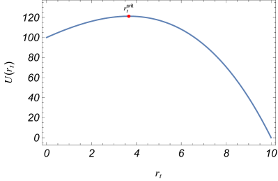
(a)

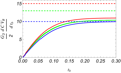
(b)

Figure 3: The left figure is a numerical plot of the effective potential $U(r_{t})$ (152) with parameters chosen as $\phi_{0}=1$, $\phi_{h}=0.5$, $r_{h}=10$. The figure on the right is a numerical plot of time-dependence of the growth rate of the bulk contributed $\mathcal{CV}_{B}$ with parameters chosen as $\phi_{0}=1$ and $r_{h}=10$. The solid and dashed curves are the growth rate and Lloyd’s bound with $\phi_{h}=0$ (blue), $\phi_{h}=0.3$ (green), $\phi_{h}=0.5$ (red).

To study the behavior of the growth rate approaching the saturation value, we can do the expansion up to the second order of the growth rate around the critical value of radius $r^{\text{crit}}_{t}$ Carmi:2017jqz :

$$\frac{d\mathcal{CV_{B}}}{dt_{b}}=\frac{2}{G_{3}}\left(\sqrt{U(r^{\text{crit}}_{t})}+\frac{U^{\prime\prime}(r^{\text{crit}}_{t})(r_{t}-r^{\text{crit}}_{t})^{2}}{4\sqrt{U(r^{\text{crit}}_{t})}}\right),$$ (153)

where at the critical point the first-order derivative vanishes. The second term $U^{\prime\prime}(r^{\text{crit}}_{t})$ in (153) is always negative since this critical point is a maximum of $U(r_{t})$. Thus, we conclude that the growth rate from the CV proposal saturates from below in both cases. This conclusion is further supported by the general time dependence of the CV growth rate in the right plot in figure 3. As observed, when two branes are rigid, the growth rate saturates the Lloyd’s bound from below. However, as fluctuations increase, Lloyd’s bound becomes gradually larger than the saturation value.

6 Summary and Discussions

In this paper, we have explored CV and CA proposals within the framework of wedge holography from both bulk and brane perspectives. From the brane perspective, it is known that the on-shell action on the branes can be effectively expressed as an Einstein-Hilbert action with an effective Newton constant Chen:2020uac ; Hernandez:2020nem ; Myers:2024zhb . We focus on the limit where two branes are situated close to one another, specifically the tensionless limit. In this limit, it is known that the AdS₃ wedge Einstein gravity reduces to JT gravity Geng:2022tfc ; Geng:2022slq . Furthermore, We consider two EOW branes with intrinsic DGP gravity. In this geometric and theoretical setup, we proceed to study holographic complexities for both rigid and fluctuating branes cases and evaluate CV and CA from both bulk and brane perspectives in the spirit of wedge holography.

In the CV proposal, while keeping branes rigid, we find the late-time growth rate of complexity precisely reproduces the result from JT gravity, augmented by the brane intrinsic contributions. We obtain consistent results from both bulk and brane perspectives. However, when the branes fluctuate, the late-time growth rate includes an additional correction term that behaves like $\frac{\phi^{2}_{h}}{\phi_{0}}$, which matches with previous work Bhattacharya:2023drv . Results from both perspectives agree on the leading order in dilaton fields.

In the CA proposal, we considered cutoffs at both the UV and behind the horizon to regularize the on-shell action Akhavan:2018wla . The CA late-time growth rate remains finite after removing these cutoffs. In the case of rigid branes, we find an exact match between our CA result and that from JT gravity, along with the brane intrinsic contributions. However, in the fluctuating branes case, we observe an extra constant correction that is independent of $\phi_{0}$. This correction comes from the joint contribution from the bulk perspective and the bulk contribution from the brane perspective. This non-trivial constant term is believed to be related to the edge modes of gravity since it is contributed mainly by the joint (corner) term. The correction term arising from fluctuations further indicates that the CV proposal is more sensitive to geometric details than the CA proposal, which could be a distinctive feature of holographic complexity and may serve as a potential trace for identifying their duals in the boundary.

Beyond our calculations on the late-time growth rates, we further analyzed these results in relation to Lloyd’s bound at late times and their general time dependence. In the CA proposal, growth rates reach Lloyd’s bound for both rigid and fluctuating branes cases, with the growth rates approaching the saturation value from above. For the CV proposal, growth rates saturate the bound in the rigid branes case. However, as the brane fluctuations increase, a gap between Lloyd’s bound and the growth rates widens, with the bound increasingly exceeding the growth rates. Furthermore, in both cases, the growth rates from the CV proposal consistently approach the saturation value from below.

Lastly, we propose several interesting directions for future research. One natural generalization is to explore holographic complexity for higher-curvature gravity Wang:2023noo ; Mandal:2022ztj ; Ghodsi:2020qqb ; Alishahiha:2017hwg ; Ding:2018ibq ; Jiang:2018sqj ; Cano:2018aqi ; An:2018dbz in the context of (higher-dimensional)wedge holography. In this paper, we focused on asymptotically AdS braneworlds; however, holographic complexity has been studied in dS braneworlds Aguilar-Gutierrez:2023tic . It is known that by tuning the brane tension, one can achieve asymptotically AdS, dS, or flat braneworlds. An intriguing direction would be to investigate the transition of holographic complexity across these different braneworlds by setting the tension at a critical value Myers:2024zhb . Additionally, examining the boundary correspondence of wedge holographic complexity presents another promising avenue for exploration. It is especially interesting to consider the SYK model, in which we may find the fingerprint of the extra constant contribution of complexity in the fluctuating branes case.

Appendix A $\text{AdS}_{3}$ black string geometry

In this section, we show how to get the foliation geometry (4) in the main text by coordinate transformations. To do so, let us start with the Poincaré patch in AdS₃ space:

$$ds^{2}=\frac{l^{2}_{3}}{z^{2}}\left(-dt^{2}+dz^{2}+dw^{2}\right),$$ (154)

where $z$ is the radial coordinate and the asymptotic boundary is located at $z\rightarrow\infty$. We can do a coordinate transformation: $z=u\sin{\mu},~w=-u\cos{\mu}$ resulting in the following metric:

$$ds^{2}=\frac{l^{2}_{3}}{\sin^{2}\mu}\left(-\frac{dt^{2}+du^{2}}{u^{2}}+d\mu^{2}\right),$$ (155)

where $0<\mu<\pi$, and $u>0$. We can then go to the global patch for each AdS₂ slice by doing the following coordinate transformations:

$$\eta=\ln(u),\ \ \ \tau=\left(\frac{2e^{-\eta}}{e^{\eta}+e^{-\eta}}\right)t.$$ (156)

The metric becomes

$$ds^{2}=\frac{1}{\sin^{2}\mu}\left(-\cosh^{2}\left(\frac{\eta}{l_{3}}\right)d\tau^{2}+d\eta^{2}+l^{2}_{3}d\mu^{2}\right),$$ (157)

where $-\infty<\eta<\infty$. Following a further coordinate transformation below:

$$y=l_{3}\log{\left(\cot{\frac{\mu}{2}}\right)},$$ (158)

we find the metric describing AdS₂ global patch slicing of AdS₃:

$$ds^{2}=dy^{2}+\cosh^{2}\left(\frac{y}{l_{3}}\right)\left(-\cosh^{2}{\eta}d\tau^{2}+d\eta^{2}\right),$$ (159)

where $-\infty<y<\infty$ and $-\infty<\eta<\infty$. By applying (158) to the metric (155), it is straightforward to transform to Poincaré patch on AdS₂ slicing of AdS₃:

$$ds^{2}=dy^{2}+l^{2}_{3}\cosh^{2}\left(\frac{y}{l_{3}}\right)\left(-\frac{dt^{2}+dx^{2}}{x^{2}}\right),$$ (160)

by applying the following coordinate transformations:

$$t=e^{r_{h}\tau}\frac{l_{3}r}{\sqrt{r^{2}-r_{h}^{2}}},\ \ \ x=e^{r_{h}\tau}\frac{l_{3}r_{h}}{\sqrt{r^{2}-r_{h}^{2}}},$$ (161)

we eventually get the AdS₂ black hole patch slicing of AdS₃:

$$ds^{2}=dy^{2}+\cosh^{2}\left(\frac{y}{l_{3}}\right)\left(-\frac{r^{2}-r_{h}^{2}}{l_{3}^{2}}d\tau^{2}+\frac{l_{3}^{2}}{r^{2}-r_{h}^{2}}dr^{2}\right).$$ (162)

This metric describes the black string metric in AdS₃.

References

- (1) J. M. Maldacena, The Large N limit of superconformal field theories and supergravity, Adv. Theor. Math. Phys. 2 (1998) 231–252, [hep-th/9711200].
- (2) S. S. Gubser, I. R. Klebanov and A. M. Polyakov, Gauge theory correlators from noncritical string theory, Phys. Lett. B 428 (1998) 105–114, [hep-th/9802109].
- (3) E. Witten, Anti-de Sitter space and holography, Adv. Theor. Math. Phys. 2 (1998) 253–291, [hep-th/9802150].
- (4) T. Takayanagi, Holographic Dual of BCFT, Phys. Rev. Lett. 107 (2011) 101602, [1105.5165].
- (5) M. Fujita, T. Takayanagi and E. Tonni, Aspects of AdS/BCFT, JHEP 11 (2011) 043, [1108.5152].
- (6) A. Karch and L. Randall, Open and closed string interpretation of SUSY CFT’s on branes with boundaries, JHEP 06 (2001) 063, [hep-th/0105132].
- (7) L. Randall and R. Sundrum, A Large mass hierarchy from a small extra dimension, Phys. Rev. Lett. 83 (1999) 3370–3373, [hep-ph/9905221].
- (8) L. Randall and R. Sundrum, An Alternative to compactification, Phys. Rev. Lett. 83 (1999) 4690–4693, [hep-th/9906064].
- (9) S. S. Gubser, AdS / CFT and gravity, Phys. Rev. D 63 (2001) 084017, [hep-th/9912001].
- (10) A. Karch and L. Randall, Locally localized gravity, JHEP 05 (2001) 008, [hep-th/0011156].
- (11) G. Yadav, Multiverse in Karch-Randall Braneworld, JHEP 03 (2023) 103, [2301.06151].
- (12) Q. Wen, M. Xu and H. Zhong, Partial entanglement entropy threads in island phase, 2408.13535.
- (13) J. Lin, Y. Lu and Q. Wen, Cutoff brane vs the Karch-Randall brane: the fluctuating case, JHEP 06 (2024) 017, [2312.03531].
- (14) S. E. Aguilar-Gutierrez, A. K. Patra and J. F. Pedraza, Entangled universes in dS wedge holography, JHEP 10 (2023) 156, [2308.05666].
- (15) S. E. Aguilar-Gutierrez, B. Craps, J. Hernandez, M. Khramtsov, M. Knysh and A. Shukla, Holographic complexity: braneworld gravity versus the Lloyd bound, JHEP 03 (2024) 173, [2312.12349].
- (16) S. E. Aguilar-Gutierrez and F. Landgren, A multiverse model in T2 dS wedge holography, JHEP 11 (2024) 122, [2311.02074].
- (17) K. K. Kim, S. Kim, J. H. Lee, C. Park and Y. Seo, End of the world perspective to BCFT, Eur. Phys. J. C 84 (2024) 530, [2309.13624].
- (18) J.-C. Chang, S. He, Y.-X. Liu and L. Zhao, Island formula in Planck brane, JHEP 11 (2023) 006, [2308.03645].
- (19) G. Yadav and H. Rathi, Yang-Baxter deformed wedge holography, Phys. Lett. B 852 (2024) 138592, [2307.01263].
- (20) D. Li and R.-X. Miao, Massless entanglement islands in cone holography, JHEP 06 (2023) 056, [2303.10958].
- (21) H. Kanda, M. Sato, Y.-k. Suzuki, T. Takayanagi and Z. Wei, AdS/BCFT with brane-localized scalar field, JHEP 03 (2023) 105, [2302.03895].
- (22) R.-X. Miao, Entanglement island and Page curve in wedge holography, JHEP 03 (2023) 214, [2301.06285].
- (23) P.-J. Hu, D. Li and R.-X. Miao, Island on codimension-two branes in AdS/dCFT, JHEP 11 (2022) 008, [2208.11982].
- (24) I. Akal, Y. Kusuki, T. Takayanagi and Z. Wei, Codimension two holography for wedges, Phys. Rev. D 102 (2020) 126007, [2007.06800].
- (25) H. Geng and A. Karch, Massive islands, JHEP 09 (2020) 121, [2006.02438].
- (26) R. Bousso and E. Wildenhain, Gravity/ensemble duality, Phys. Rev. D 102 (2020) 066005, [2006.16289].
- (27) R.-X. Miao, An Exact Construction of Codimension two Holography, JHEP 01 (2021) 150, [2009.06263].
- (28) H. Geng, Aspects of AdS2 quantum gravity and the Karch-Randall braneworld, JHEP 09 (2022) 024, [2206.11277].
- (29) H. Geng, A. Karch, C. Perez-Pardavila, S. Raju, L. Randall, M. Riojas et al., Jackiw-Teitelboim Gravity from the Karch-Randall Braneworld, Phys. Rev. Lett. 129 (2022) 231601, [2206.04695].
- (30) A. Almheiri, D. Marolf, J. Polchinski and J. Sully, Black Holes: Complementarity or Firewalls?, JHEP 02 (2013) 062, [1207.3123].
- (31) J. Maldacena and L. Susskind, Cool horizons for entangled black holes, Fortsch. Phys. 61 (2013) 781–811, [1306.0533].
- (32) S. Ryu and T. Takayanagi, Holographic derivation of entanglement entropy from AdS/CFT, Phys. Rev. Lett. 96 (2006) 181602, [hep-th/0603001].
- (33) L. Susskind, Entanglement is not enough, Fortsch. Phys. 64 (2016) 49–71, [1411.0690].
- (34) L. Susskind, Computational Complexity and Black Hole Horizons, Fortsch. Phys. 64 (2016) 24–43, [1403.5695].
- (35) D. Stanford and L. Susskind, Complexity and Shock Wave Geometries, Phys. Rev. D 90 (2014) 126007, [1406.2678].
- (36) A. R. Brown, D. A. Roberts, L. Susskind, B. Swingle and Y. Zhao, Holographic Complexity Equals Bulk Action?, Phys. Rev. Lett. 116 (2016) 191301, [1509.07876].
- (37) A. R. Brown, D. A. Roberts, L. Susskind, B. Swingle and Y. Zhao, Complexity, action, and black holes, Phys. Rev. D 93 (2016) 086006, [1512.04993].
- (38) N. Engelhardt and r. Folkestad, General bounds on holographic complexity, JHEP 01 (2022) 040, [2109.06883].
- (39) L. V. Iliesiu, M. Mezei and G. Sárosi, The volume of the black hole interior at late times, JHEP 07 (2022) 073, [2107.06286].
- (40) R.-Q. Yang, Y.-S. An, C. Niu, C.-Y. Zhang and K.-Y. Kim, What kind of “complexity” is dual to holographic complexity?, Eur. Phys. J. C 82 (2022) 262, [2011.14636].
- (41) E. Rabinovici, A. Sánchez-Garrido, R. Shir and J. Sonner, A bulk manifestation of Krylov complexity, JHEP 08 (2023) 213, [2305.04355].
- (42) S. Chapman, D. Ge and G. Policastro, Holographic Complexity for Defects Distinguishes Action from Volume, JHEP 05 (2019) 049, [1811.12549].
- (43) P. Braccia, A. L. Cotrone and E. Tonni, Complexity in the presence of a boundary, JHEP 02 (2020) 051, [1910.03489].
- (44) W. Israel, Singular hypersurfaces and thin shells in general relativity, Nuovo Cim. B 44S10 (1966) 1.
- (45) C. W. Misner, K. S. Thorne and J. A. Wheeler, Gravitation. W. H. Freeman, San Francisco, 1973.
- (46) J. Maldacena, D. Stanford and Z. Yang, Conformal symmetry and its breaking in two dimensional Nearly Anti-de-Sitter space, PTEP 2016 (2016) 12C104, [1606.01857].
- (47) H. Z. Chen, R. C. Myers, D. Neuenfeld, I. A. Reyes and J. Sandor, Quantum Extremal Islands Made Easy, Part I: Entanglement on the Brane, JHEP 10 (2020) 166, [2006.04851].
- (48) H. Geng, A. Karch, C. Perez-Pardavila, L. Randall, M. Riojas, S. Shashi et al., Constraining braneworlds with entanglement entropy, SciPost Phys. 15 (2023) 199, [2306.15672].
- (49) R. C. Myers, S.-M. Ruan and T. Ugajin, Double holography of entangled universes, JHEP 07 (2024) 035, [2403.17483].
- (50) C. Fefferman and C. R. Graham, Conformal invariants, in The Mathematical Heritage of Élie Cartan (Lyon, 1984), Astérisque, Numero Hors Serie (1985) 95–116.
- (51) C. Fefferman and C. R. Graham, The ambient metric, Ann. Math. Stud. 178 (2011) 1–128, [0710.0919].
- (52) J. Hernandez, R. C. Myers and S.-M. Ruan, Quantum extremal islands made easy. Part III. Complexity on the brane, JHEP 02 (2021) 173, [2010.16398].
- (53) A. Bhattacharya, A. Bhattacharyya and A. K. Patra, Holographic complexity of Jackiw-Teitelboim gravity from Karch-Randall braneworld, 2304.09909.
- (54) A. Belin, R. C. Myers, S.-M. Ruan, G. Sárosi and A. J. Speranza, Does Complexity Equal Anything?, Phys. Rev. Lett. 128 (2022) 081602, [2111.02429].
- (55) A. Belin, R. C. Myers, S.-M. Ruan, G. Sárosi and A. J. Speranza, Complexity equals anything II, JHEP 01 (2023) 154, [2210.09647].
- (56) R. C. Myers and S.-M. Ruan, Complexity Equals (Almost) Anything, 3, 2024. 2403.17475.
- (57) M. Alishahiha, On complexity of Jackiw–Teitelboim gravity, Eur. Phys. J. C 79 (2019) 365, [1811.09028].
- (58) A. R. Brown, H. Gharibyan, H. W. Lin, L. Susskind, L. Thorlacius and Y. Zhao, Complexity of Jackiw-Teitelboim gravity, Phys. Rev. D 99 (2019) 046016, [1810.08741].
- (59) D. Carmi, R. C. Myers and P. Rath, Comments on Holographic Complexity, JHEP 03 (2017) 118, [1612.00433].
- (60) A. Chamblin, S. W. Hawking and H. S. Reall, Brane world black holes, Phys. Rev. D 61 (2000) 065007, [hep-th/9909205].
- (61) A. Akhavan, M. Alishahiha, A. Naseh and H. Zolfi, Complexity and Behind the Horizon Cut Off, JHEP 12 (2018) 090, [1810.12015].
- (62) L. Lehner, R. C. Myers, E. Poisson and R. D. Sorkin, Gravitational action with null boundaries, Phys. Rev. D 94 (2016) 084046, [1609.00207].
- (63) T. Takayanagi and K. Tamaoka, Gravity Edges Modes and Hayward Term, JHEP 02 (2020) 167, [1912.01636].
- (64) S. Lloyd, Ultimate physical limits to computation, Nature 406 (2000) 1047–1054.
- (65) S. Chapman, H. Marrochio and R. C. Myers, Holographic complexity in Vaidya spacetimes. Part II, JHEP 06 (2018) 114, [1805.07262].
- (66) D. Carmi, S. Chapman, H. Marrochio, R. C. Myers and S. Sugishita, On the Time Dependence of Holographic Complexity, JHEP 11 (2017) 188, [1709.10184].
- (67) X. Wang, R. Li and J. Wang, Generalized volume complexity in Gauss-Bonnet gravity: Constraints and phase transitions, Phys. Rev. D 108 (2023) 126018, [2307.12530].
- (68) T. Mandal, A. Mitra and G. S. Punia, Action complexity of charged black holes with higher derivative interactions, Phys. Rev. D 106 (2022) 126017, [2205.11201].
- (69) A. Ghodsi, S. Qolibikloo and S. Karimi, Holographic complexity in general quadratic curvature theory of gravity, Eur. Phys. J. C 80 (2020) 920, [2005.08989].
- (70) M. Alishahiha, A. Faraji Astaneh, A. Naseh and M. H. Vahidinia, On complexity for F(R) and critical gravity, JHEP 05 (2017) 009, [1702.06796].
- (71) Y.-C. Ding and T. Wang, Action growth rates of black holes in the Chern-Simons modified gravity, 1811.08113.
- (72) J. Jiang and H. Zhang, Surface term, corner term, and action growth in gravity theory, Phys. Rev. D 99 (2019) 086005, [1806.10312].
- (73) P. A. Cano, R. A. Hennigar and H. Marrochio, Complexity Growth Rate in Lovelock Gravity, Phys. Rev. Lett. 121 (2018) 121602, [1803.02795].
- (74) Y.-S. An, R.-G. Cai and Y. Peng, Time Dependence of Holographic Complexity in Gauss-Bonnet Gravity, Phys. Rev. D 98 (2018) 106013, [1805.07775].