Transverse densities of the energy-momentum tensor and the gravitational form factors the pion

Abstract

We present general features of the transverse densities of the stress-energy-momentum tensor $\Theta^{\mu\nu}$ in the pion. We show positivity of the transverse density of $\Theta^{++}$ (analogous to the positivity of the transverse density of the electromagnetic current $J^{+}$) and discuss its consequences in conjunction with analyticity and quark-hadron duality, as well as the connection to $\pi\pi$ scattering at low energies. Our analysis takes into account the perturbative QCD effects, dominating at high momenta (or low transverse coordinate $b$), the effects of Chiral Perturbation Theory, dominating at low momenta (high $b$), and meson dominance in the intermediate region. We incorporate constraints form analyticity, leading to sum rules for the spectral densities of the corresponding form factors, which i.a. are relevant for the high-momentum (or the low-$b$) asymptotics. With the obtained high- and low-$b$ behavior, we deduce that the scalar (trace-anomaly) gravitational transverse density $\Theta^{\mu}_{\mu}(b)$ must change sign, unlike the case of the positive definite $J^{+}(b)$ or $\Theta^{++}(b)$. We also discuss the transverse pressure in the pion, which is positive and singular at low $b$, and negative at high $b$, in harmony with the stability criterion. The results for the form factors for space-like momenta are compared to the recent lattice QCD data.

1 Remembrance

The horn signal used to call everyone for coffee to the window-less social room of the Theoretical Physics Department II of the Ruhr Universität in Bochum. There, among all the friends of the group headed by dearest Klaus Goeke, many brilliant ideas were coined and discussed, with the three friends commemorated in this volume playing leading roles. Out of the many concepts that originated there, those from Maxim and collaborators continue to be particularly important in our humble research. In particular, the $D$ (druck) term [1] in the generalized parton distributions, hence in the gravitational form factors (GFFs) related to matrix elements of the stress-energy momentum (SEM) tensor, as well as the interpretation of the matrix elements of the energy-momentum tensor via the physically intuitive mechanistic properties of hadrons [2, 3], are at the core of in this paper.

2 Stress-energy-momentum tensor in the pion

2.1 Introduction and scope

The SEM tensor appears as a universal Noether current in any Quantum Field Theory textbook since the early days. It has played a decisive role in the theoretical understanding of scale invariance and its violations [4]. Yet, phenomenological implications for hadronic physics have been less frequent, mainly due to the impossibility of making direct experimental or ab initio determinations. The very first mention of the gravitational form factors that we are aware of was within the context of $NN$ interactions, in order to characterize the tensor meson exchange [5]. Pagels made the first study based on analyticity and final state interactions [6]. The proper tensor decomposition was written down by Raman [7]. Coupled channel analyses have been pioneered in Refs. [8, 9], whereas a Chiral Perturbation Theory ($\chi$PT) setup was proposed in [10].

The recent activity in GFFs of the pion has been largely spurred by the release of accurate lattice QCD data by the MIT group [11, 12], obtained for all the parton species and close to the physical point, with $m_{\pi}=170$ MeV. This ameliorates the seminal studies of the quark parts [13, 14], recently repeated for $m_{\pi}=250$ MeV [15], of the gluonic parts [16], or the trace anomaly component [17] at large $m_{\pi}$. On the experimental side, a method of extracting GFFs from the $\gamma\gamma^{\ast}\to\pi^{0}\pi^{0}$ data [18] was developed in [19], with further prospects at Super-KEKB and ILC, where the generalized distribution amplitudes of the pion could be investigated.

Model calculations of the pion GFFs have been carried out in various approaches, including [20, 21, 22, 23, 24, 25, 26, 27, 28, 29, 30, 31, 32, 33, 34, 35]. In this paper we extend the meson dominance model [36, 37], applied successfully to the lattice data of [11, 12] (our techique was later repeated in [38]), by incorporating explicitly the perturbative QCD (pQCD), computed recently [39, 40], as well as the $\chi$PT [10] pieces. Our analysis is done with the help of the dispersion relations, which allows us to preserve analyticity when combining various contribution (meson dominance, pQCD, $\chi$PT) and to satisfy all the required sum rules.

We obtain the transverse densities of the energy-momentum tensor in the pion and discuss their general features, such as the singular limits at a low transverse coordinate $b$, stemming from pQCD, and the high-$b$ asymptotics following from the threshold behavior of the $\pi\!-\!\pi$ scattering. For the scalar (trace anomaly) transverse density, the opposite sign of the low- and high-$b$ limits proves that it has to change sign as a function of $b$. This is not the case of the charge or the tensor GFFs, which are positive definite. Finally, we discuss the transverse pressure inside the pion, following from the gravitational transverse densities.

2.2 The energy momentum tensor

We will use the Hilbert definition of the SEM tensor via the coupling to gravity, which in the QCD case coincides with the Belinfante-Rosenfeld definition [41] (see also Appendix E of [42]),

$$\Theta^{\mu\nu}=\tfrac{i}{4}\bar{\Psi}\left[\gamma^{\mu}\overleftrightarrow{D}^{\mu}\!+\!\gamma^{\nu}\overleftrightarrow{D}^{\mu}\right]\Psi-F^{\mu\lambda a}F^{\nu}_{\lambda a}+\tfrac{1}{4}g^{\mu}F^{\sigma\lambda a}F_{\sigma\lambda a}+\Theta_{\rm GF-EOM}^{\mu\nu},$$ (1)

where in the quantized case one has in addition the gauge-fixing and the equations-of-motion terms. This object is local, symmetric, $\Theta^{\mu\nu}=\Theta^{\nu\mu}$, conserved $\partial_{\mu}\Theta^{\mu\nu}=0$, and from the Lorentz group can be irreducibly decomposed as a sum of a traceful and traceless parts. It is a highly singular operator which requires renormalization. The trace can be written as an anomalous divergence of the dilatation current, $D^{\mu}=x_{\nu}\Theta^{\mu\nu}$, related unambiguously to the scale invariance breaking [41], namely

$$\Theta\equiv\Theta^{\mu}_{\mu}=\frac{\beta(\alpha)}{4\alpha}{G^{\mu\nu}}^{2}+[1+\gamma_{m}(\alpha)]\sum_{f}m_{f}\bar{q}_{f}q_{f}.$$ (2)

Here $\beta(\alpha)=\mu^{2}d\alpha/d\mu^{2}=-\alpha[\beta_{0}(\alpha/4\pi)+{\cal O}(\alpha^{2})]<0$ is the QCD beta function with $\beta_{0}=(11N_{c}-2N_{F})/3$, $N_{c}$ is the number of colors, $N_{F}$ is the number of flavors, $\gamma_{m}(\alpha)=2\alpha/\pi+{\cal O}(\alpha^{2})$ is the quark mass anomalous dimension, and $f$ enumerates active flavors. One has $\alpha(t)=(4\pi/\beta_{0})/\ln\left(-t/\Lambda_{\rm QCD}^{2}\right)$ with $\alpha(t)$ real for $t=-Q^{2}<0$. We take $\Lambda_{Q}=225$ MeV and $N_{F}=3$ in our numerical studies presented later on.

2.3 Raman decomposition

The standard tensor decomposition of the SEM tensor matrix element in the pion state of isospin $a,b$ is

$$\hskip-19.91692pt\langle\pi^{a}(p^{\prime})|\Theta^{\mu\nu}(0)|\pi^{b}(p)\rangle=\delta^{ab}\left[2P^{\mu}P^{\nu}A(q^{2})+\frac{1}{2}(q^{\mu}q^{\nu}-g^{\mu\nu}q^{2})D(q^{2})\right],$$ (3)

where $P=\tfrac{1}{2}(p^{\prime}+p)$, $q=p^{\prime}-p$, and $A$ and $D$ are the gravitational form factors. For the electromagnetic current, $J_{Q}^{\mu}=\bar{\Psi}\gamma^{\mu}Q\Psi$, one has

$$\langle\pi^{\pm}(p^{\prime})|J_{Q}^{\mu}(0)|\pi^{\pm}(p)\rangle=\pm 2P^{\mu}F(q^{2}),$$ (4)

where $F$ is the charge form factor, to which we shall make frequent references in the context of our discussion of GFFs for comparison purposes.

The proper decomposition into a sum of two separately conserved irreducible tensors of a well-defined total angular momentum, $J^{PC}=0^{++}$ (scalar) and $2^{++}$ (tensor), has the form [7]

$$\Theta^{\mu\nu}=\Theta_{S}^{\mu\nu}+\Theta_{T}^{\mu\nu},\;\;\Theta_{S}^{\mu\nu}=\frac{1}{3}Q^{\mu\nu}\Theta,$$ (5)

$$\Theta_{T}^{\mu\nu}=\Theta^{\mu\nu}-\frac{1}{3}Q^{\mu\nu}\Theta=2\left[P^{\mu}P^{\nu}-\frac{P^{2}}{3}Q^{\mu\nu}\right]A,$$

where $Q^{\mu\nu}\equiv g^{\mu\nu}-{q^{\mu}q^{\nu}}/{q^{2}}$ (for brevity, we drop here the argument of the GFFs, which is $q^{2}$). This decomposition implements a separate conservation of the scalar and tensor parts, $q_{\mu}\Theta_{S}^{\mu\nu}=q_{\mu}\Theta_{T}^{\mu\nu}=0$, unlike the and often used naive decomposition with $\Theta_{T}^{\mu\nu}=\Theta^{\mu\nu}-\tfrac{1}{4}g^{\mu\nu}\Theta$ and $\Theta_{S}^{\mu\nu}=\tfrac{1}{4}g^{\mu\nu}\Theta$, which violated the separate conservation property, since, e.g., $q_{\mu}\Theta_{S}^{\mu\nu}=q^{\nu}\Theta$. The Raman separation of the GFFs, when promoted to the operator level in QCD, also has the feature that the trace of SEM is singular and requires renormalization, cf. Eq. (2). From this point of view, $\Theta$ and $A$, carrying good $J^{PC}$ quantum numbers, should be regarded as the basic form factors [36], whereas $D$ mixes the quantum numbers and is given as a secondary quantity (albeit naturally appearing in the mechanistic properties [2, 3]) by the combination

$$D=-\frac{2}{3q^{2}}\left[\Theta-\left(2m_{\pi}^{2}-\tfrac{1}{2}\,q^{2}\right)A\right].$$ (6)

2.4 Meson dominance vs lattice data

At a phenomenological level, we have found that from the MIT lattice data [11] at $m_{\pi}=170$ MeV one can infer, using $\chi$PT to NLO, that in the range $0<-t<2~{\rm GeV}^{2}$ and for the physical $m_{\pi}=140$ MeV the GFFs can be very satisfactorily described in the single resonance saturation picture proposed long ago [10],

$$\Theta(t) = 2m_{\pi}^{2}+\frac{tm_{\sigma}^{2}}{m_{\sigma}^{2}-t}$$ (7)

$$A(t) = \frac{m_{f_{2}}^{2}}{m_{f_{2}}^{2}-t},$$ (8)

with $m_{\sigma}=0.63(6)$ GeV and $m_{f_{2}}=1.27(4)$ GeV [36]. The gravitational low energy constants $L_{11,12,13}$, as well as the corresponding value of the $D$-term, $D(0)=-0.95(3)$, have been extracted thereof [37].

3 Transverse densities

3.1 Preliminary

The transverse densities of hadrons in the infinite momentum frame were advocated in [43, 44, 45, 46, 47, 48] as proper objects relating to the probabilistic interpretation of the parton distributions. In particular, the transverse electromagnetic (charge) density can be shown to be manifestly positive definite [46, 49, 45]. Likewise, the transverse $\Theta^{++}$ distribution is also positive definite (for any hadronic state), as we will demonstrate below. Moreover, as argued in [50], for spin-0 mesons such as the pion, the 3D Breit-frame densities are not related to the transverse densities via the Abel transform, as is the case for the nucleon [51], hence they acquire even more significance.

3.2 Light-cone kinematics for plane waves

We take the conventions $p^{\pm}=(p^{0}\pm p^{3})/\sqrt{2}=p_{\mp}$, such that $x\cdot p=p^{+}x^{-}+p^{-}x^{+}-p_{\perp}\cdot x_{\perp}$ and $d^{4}p=dp^{+}dp^{-}d^{2}p_{\perp}$. Also, $g^{++}=g^{--}=0$ and $g^{+-}=g^{-+}=1$. Assume the momentum transfer has only the $q_{\perp}$ component, i.e. $q^{+}=q^{-}=0$. The momenta of the pions in the chosen frame (IMBF, infinite momentum Breit frame) are therefore

$$p^{+}={p^{+}}^{\prime}=P^{+},\;\;p^{-}={p^{-}}^{\prime}=\frac{\tfrac{1}{4}q_{\perp}^{2}+m_{\pi}^{2}}{2{P^{+}}},\;\;p_{\perp}=-{p_{\perp}}^{\prime}=-\tfrac{1}{2}q_{\perp}.$$ (9)

In the light front quantization (see, e.g., [48] and references therein), the states on the mass shell are labeled as $|p^{+},p_{\perp}\rangle$. They fulfill the completeness relation

$$\int\frac{dp^{+}dp^{-}d^{2}p_{\perp}}{(2\pi)^{4}}2\pi\theta(p^{+})\,\delta(2p^{+}p^{-}-p_{\perp}^{2}-m_{\pi}^{2})|p^{+},p_{\perp}\rangle\langle p^{+},p_{\perp}|=1,$$ (10)

corresponding to $p^{-}=(p_{\perp}^{2}+m_{\pi}^{2})/2p^{+}$ and $p^{+}>0$, and the invariant normalization

$$\langle p^{+},p_{\perp}|{p^{+}}^{\prime},{p_{\perp}}^{\prime}\rangle=2p^{+}(2\pi)^{3}\delta({p^{+}}-{p^{+}}^{\prime})\delta^{2}(p_{\perp}-{p_{\perp}}^{\prime}),$$ (11)

which implies the rule to divide with $\sqrt{2p^{+}}$ for the initial and $\sqrt{{2p^{+}}^{\prime}}$ for the final state.

The matrix element of the $+$ component of the electromagnetic current is $2p^{+}F(q_{\perp}^{2})$, and the factor of $2p^{+}$ cancels with the one originating from the normalization (11) (here this is similar to the instant form case). One defines the transverse charge density as

$$F^{+}(b)=\int\frac{d^{2}q_{\perp}}{(2\pi)^{2}}e^{-iq_{\perp}\cdot b}F(q_{\perp}^{2}).$$ (12)

Note that $F^{+}(b)$ corresponds to the $+$ component of the current. The $\perp$ components of the current vanish identically in IMBF. For the $-$ component of the current, we acquire the factor $P^{-}/P^{+}$ in the integrand, which vanishes in IMBF when $P^{+}\to\infty$.

Next, let us look at the $++$ component of Eq. (3),

$$\Theta^{++}(b)=\int\frac{d^{2}q_{\perp}}{2P^{+}(2\pi)^{2}}e^{-iq_{\perp}\cdot b}\,2{P^{+}}^{2}A(q_{\perp}^{2})=P^{+}A(b),$$ (13)

which gives a simple interpretation to $A(b)$ as the relative distribution of $P^{+}$ in the transverse coordinate space. Obviously, $\int d^{2}b\,\Theta^{++}(b)=P^{+}$. For the $+-$ component we have

$$\Theta^{+-}(b)=\int\frac{d^{2}q_{\perp}}{2P^{+}(2\pi)^{2}}e^{-iq_{\perp}\cdot b}\left[2{P^{+}}P^{-}A(q_{\perp}^{2})+\frac{1}{2}q_{\perp}^{2}D(q_{\perp}^{2})\right],$$ (14)

where we have used $g^{+-}=1$. With the kinematics (9) we get immediately

$$\Theta^{+-}(b)=\frac{1}{2P^{+}}\int\frac{d^{2}q_{\perp}}{(2\pi)^{2}}e^{-iq_{\perp}\cdot b}\left[(m_{\pi}^{2}+\tfrac{1}{4}q_{\perp}^{2})A(q_{\perp}^{2})+\frac{1}{2}q_{\perp}^{2}D(q_{\perp}^{2})\right].$$ (15)

The $--$ component is strongly suppressed, $\sim 1/P_{+}^{3}$, and involves only $A$ in the chosen frame. The transverse components are

$$\Theta^{ij}(b)=\frac{1}{2P^{+}}\int\frac{d^{2}q_{\perp}}{(2\pi)^{2}}e^{-iq_{\perp}\cdot b}\frac{1}{2}\left[q_{\perp}^{i}q_{\perp}^{j}-\delta^{ij}q_{\perp}^{2}\right]D(q_{\perp}^{2})=$$

$$~~~~~\delta^{ij}p(b)+\left[\frac{b^{i}b^{j}}{b^{2}}-\frac{1}{2}\delta^{ij}\right]s(b),$$ (16)

where $p(b)$ is the transverse pressure and $s(b)$ denotes the transverse shear forces. The trace GFF is

$$\Theta^{\mu}_{\mu}(b)=2\Theta^{+-}(b)-\Theta^{11}(b)-\Theta^{22}(b)=$$

$$~~~~~~~\frac{1}{2P^{+}}\int\frac{d^{2}q_{\perp}}{(2\pi)^{2}}e^{-iq_{\perp}\cdot b}\left[2(m_{\pi}^{2}+\tfrac{1}{4}q_{\perp}^{2})A(q_{\perp}^{2})+\frac{3}{2}q_{\perp}^{2}D(q_{\perp}^{2})\right]$$

$$~~=\frac{1}{2P^{+}}\int\frac{d^{2}q_{\perp}}{(2\pi)^{2}}e^{-iq_{\perp}\cdot b}\Theta(q_{\perp}^{2})=\frac{1}{2P^{+}}\Theta(b).$$ (17)

The normalizations are $\int d^{2}b\,\Theta^{\mu}_{\mu}(b)=m_{\pi}^{2}/P^{+}$ and $\int d^{2}b\,\Theta(b)=2m_{\pi}^{2}$. In the above formulas the normalization factors of $1/(2P^{+})$ factor out of the Fourier transforms, in contrast to the instant form quantization, where $1/(2P^{0})$ = $1/(2\sqrt{m_{\pi}^{2}+q_{\perp}^{2}/4})$ remains inside the integral and largely affects the interpretation, in particular for light hadrons.

3.3 Intrinsic properties vs form factors

From a Quantum Mechanical point of view, intrinsic physical properties are obtained as expectation values of self-adjoint operators in a normalizable quantum mechanical state $|\psi\rangle$, $\langle A\rangle_{\psi}=\langle\psi|A|\psi\rangle$. However, form factors by themselves are non-diagonal matrix elements between plane waves. The use of the light-cone (LC) coordinates has been promoted as a way to provide a proper definition of intrinsic properties related to form factors, fully compatible with the probabilistic interpretation. To establish the connection, instead of the plane waves one considers wave packets, which in LC coordinates and for the pion read

$$|\phi\rangle=\int\frac{d^{2}p_{\perp}dp^{+}}{(2\pi)^{3}2p^{+}}\tilde{\phi}(p_{\perp},p^{+})|p_{\perp},p^{+}\rangle.$$ (18)

From here we have the scalar product

$$\langle\phi|\psi\rangle = \int\frac{d^{2}p_{\perp}dp^{+}}{(2\pi)^{3}2p^{+}}\tilde{\phi}(p_{\perp},p^{+})^{*}\tilde{\psi}(p_{\perp},p^{+})$$ (19)

$$= \int d^{2}x_{\perp}dx^{-}\phi(x_{\perp},x^{-})^{*}\psi(x_{\perp},x^{-}).$$

The coordinate and momentum representations are related via the Fourier transform,

$$\psi(x_{\perp},x^{-})=\int\frac{d^{2}p_{\perp}dp^{+}}{\sqrt{(2\pi)^{3}2p^{+}}}\tilde{\psi}(p_{\perp},p^{+})e^{i(x_{\perp}\cdot p_{\perp}-p^{+}x^{-})}.$$ (20)

In [44] wave packets localized sharply around $p_{z}\to\infty$ were considered. An equivalent way is to integrate over the $x^{-}$ coordinate in the local operator, and define the transverse wave packet distribution in the transverse coordinate $b=x_{\perp}$,

$$n_{\psi}(b)=\int dx^{-}|\psi(b,x^{-})|^{2}=\int_{0}^{\infty}\frac{dp^{+}}{4\pi p^{+}}\left|\int\frac{d^{2}p_{\perp}}{(2\pi)^{2}}e^{ib\cdot p_{\perp}}\tilde{\psi}(p_{\perp},p^{+})\right|^{2}.$$ (21)

For local operators, we consider the $x^{+}=0$ quantization surface. Using translational invariance, $O(x)=e^{iP\cdot x}O(0)e^{-iP\cdot x}$, and after some straightforward manipulations, one obtains the intuitive formula for the expectation value of the electromagnetic current $J^{\mu}$,

$$\langle\psi|\int dx^{-}J^{+}(b,x^{-})|\psi\rangle = \int d^{2}b^{\prime}n_{\psi}(b-b^{\prime})F(b^{\prime}),$$ (22)

where $F(b)$ is the Fourier transform of the charge form factor in the space-like momentum space,

$$F(b)=\int\frac{d^{2}q_{\perp}}{(2\pi)^{2}}F(-q_{\perp}^{2})e^{-iq_{\perp}\cdot b}.$$ (23)

Next, we define

$$n^{+}_{\psi}(b) = \int dx^{-}\psi^{*}(b,x^{-})i\partial^{+}\psi(b,x^{-})$$ (24)

$$= \int_{0}^{\infty}\frac{dp^{+}}{4\pi p^{+}}p^{+}\left|\int\frac{d^{2}p_{\perp}}{(2\pi)^{2}}e^{ib\cdot p_{\perp}}\tilde{\psi}(p_{\perp},p^{+})\right|^{2}$$

to obtain, for the quark part $\Theta_{q}^{++}$,

$$\langle\psi|\int dx^{-}\Theta_{q}^{++}(b,x^{-})|\psi\rangle = \int d^{2}b^{\prime}n_{\psi}^{+}(b-b^{\prime})A_{q}(b^{\prime}),$$ (25)

where

$$A_{q}(b)=\int\frac{d^{2}q_{\perp}}{(2\pi)^{2}}A_{q}(-q_{\perp}^{2})e^{-iq_{\perp}\cdot b}.$$ (26)

Obviously, for a localized wave packet $n_{\psi}(b)\to\delta^{(2)}(b)$ and $n^{+}_{\psi}(b)\to p^{+}\delta^{(2)}(b)$, hence one has

$$\hskip-19.91692pt\langle\psi|\int dx^{-}J^{+}(b,x^{-})|\psi\rangle\to F(b),\;\;\;\langle\psi|\int dx^{-}\Theta^{++}(b,x^{-})|\psi\rangle=P^{+}A(b),$$ (27)

in accordance with Eqs. (12) and (13).

3.4 Positivity

In QCD, the EM current and SEM in LC coordinates and with the gauge $A^{+}=0$ (which is ghost free), one has

$$J^{+} = \Psi_{+}^{\dagger}Q\Psi_{+},$$

$$\Theta_{q}^{++} = \frac{i}{2}\left(\Psi^{\dagger}_{+}\partial^{+}\Psi_{+}-\partial^{+}\Psi_{+}^{\dagger}\Psi_{+}\right),\;\;\;\Theta_{g}^{++}=(\partial^{+}A^{a}_{\perp})^{2},$$

$$\Theta^{++} = \Theta_{q}^{++}+\Theta_{g}^{++}.$$ (28)

Here $Q$ is the electric charge, $\Psi_{\pm}={\cal P}_{\pm}\Psi$, where ${\cal P}_{\pm}=\gamma^{0}\gamma^{\pm}$ are orthogonal projection operators satisfying ${\cal P}_{+}+{\cal P}_{-}=1$, ${\cal P}_{\pm}^{2}={\cal P}_{\pm}={\cal P}_{\pm}^{\dagger}$ and ${\cal P}_{\pm}{\cal P}_{\mp}=0$, and the $A^{a\mu}$ is the gluon field. We note that the gluon component, $\Theta_{g}^{++}$, is manifestly positive definite. Importantly, the sum of the quark and gluon parts is renormalization group invariant.

The field expansion for the quark field in the transverse coordinate space [45] at $x^{+}=0$ is

$$q_{+}(b,x^{-})=\int_{0}^{\infty}\frac{dp^{+}}{4\pi p^{+}}\sum_{\lambda} [b_{\lambda}(b,p^{+})u_{\lambda,+}(p^{+})e^{-ip^{+}x^{-}}$$ (29)

$$+d_{\lambda}^{\dagger}(b,p^{+})v_{\lambda,+}(p^{+})e^{ip^{+}x^{-}}],$$

with $b_{\lambda}^{\dagger}(b,p^{+})$ and $d_{\lambda}^{\dagger}(b,p^{+})$ denoting the particle and antiparticle creation operators with LC helicity $\lambda$, respectively. Then

$$\int dx^{-}q_{+}^{+}q_{+} = \sum_{\lambda}\int\frac{dp^{+}}{4\pi p^{+}}\left[n(b,p^{+})-\bar{n}_{\lambda}(b,p^{+})\right],$$

$$\int dx^{-}q_{+}^{+}i\partial^{+}q_{+} = \sum_{\lambda}\int\frac{dp^{+}}{4\pi p^{+}}\left[p^{+}n_{\lambda}(b,p^{+})-p^{+}\bar{n}_{\lambda}(b,p^{+})\right],$$ (30)

with $n_{\lambda}(b,p^{+})=b^{\dagger}_{\lambda}(b,p^{+})b_{\lambda}(b,p^{+})$ and $\bar{n}_{\lambda}(b,p^{+})=d^{\dagger}_{\lambda}(b,p^{+})d_{\lambda}(b,p^{+})$ denoting the particle and antiparticle number operators, respectively. Thus, for $\pi^{+}=u\bar{d}$,

$$\int dx^{-}J^{+}(b,x^{-})\underbrace{\to}_{\pi^{+}}\sum_{\lambda}\int\frac{dp^{+}}{4\pi p^{+}}\left[\frac{2}{3}n_{u,\lambda}(b,p^{+})+\frac{1}{3}n_{\bar{d},\lambda}(b,p^{+})\right],$$ (31)

since generally $q_{+}^{\dagger}q_{+}$ is positive for quarks and negative for antiquarks. Thus (31), and consequently $F(b)$, are positive definite.

For $\Theta_{q}^{++}$one also finds positivity,

$$\hskip-56.9055pt\int dx^{-}\frac{i}{2}\left(\Psi^{\dagger}_{+}\partial^{+}\Psi_{+}-\partial^{+}\Psi_{+}^{\dagger}\Psi_{+}\right)=i\int dx^{-}\Psi^{\dagger}_{+}\partial^{+}\Psi_{+}$$

$$\underbrace{\to}_{\pi^{+}} \sum_{\lambda}\int\frac{dp^{+}}{4\pi p^{+}}\left[p^{+}n_{u,\lambda}(b,p^{+})+p^{+}n_{\bar{d},\lambda}(b,p^{+})\right]$$ (32)

To summarize this Section, both $F(b)$ and $A(b)$ are intrinsic properties of the pion which are positive definite. This allows to interpret $F(b)$ as the transverse charge distribution, whereas $A(b)$ is the transverse $p^{+}$ distribution in the pion. Note that these two distributions do not contain an interacting piece. One should keep in mind that the formulas and their interpretation as a whole depend crucially on the LC kinematics and the gauge $A^{+}=0$. We will show below that the parton-hadron duality makes the positivity conditions non-trivial, having important implications for the $\pi\pi$ scattering in the elastic region, which must be attractive in the corresponding $J^{PC}$ channels.

In each of the considered channels, $f=F,A,\Theta$, the transverse densities are defined as the Fourier-Bessel transforms

$$f(b)=\int\frac{d^{2}q_{\perp}}{(2\pi)^{2}}e^{-iq_{\perp}\cdot b}f(q_{\perp}^{2})=\int\frac{q_{\perp}dq_{\perp}}{2\pi}J_{0}(bq_{\perp})f(q_{\perp}^{2}),$$ (33)

where $J_{0}(z)$ is a Bessel function.

4 Dispersion relations and sum rules

4.1 General properties

All the considered form factors vanish sufficiently fast at large space-like momenta, hence satisfy the unsubtracted dispersion relations

$$f(-Q^{2})=\frac{1}{\pi}\int_{4m_{\pi}^{2}}^{\infty}ds\frac{{\rm Im}f(s)}{s+Q^{2}},$$ (34)

where $Q^{2}=-q^{2}=-t$ is the space-like momentum transfer squared. The relations make sense, as asymptotically ${\rm Im}\,f(s)$ tends to zero sufficiently fast (see the following) and the integrals converge. For $f=F$ or $f=A$, one has the conditions $f(0)=1$ and $\lim_{Q^{2}\to\infty}Q^{2}f(Q^{2})=0$, which are equivalent to the two sum rules

$$\frac{1}{\pi}\int_{4m_{\pi}^{2}}^{\infty}ds\frac{{\rm Im}f(s)}{s}=1,$$ (35)

$$\frac{1}{\pi}\int_{4m_{\pi}^{2}}^{\infty}ds\,{\rm Im}f(s)=0.$$ (36)

For the scalar part of the gravitational form factor, since $\Theta(0)=2m_{\pi}^{2}$, we get the mass sum rule

$$\frac{1}{\pi}\int_{4m_{\pi}^{2}}^{\infty}ds\frac{{\rm Im}\Theta(s)}{s}=2m_{\pi}^{2}.$$ (37)

The once-subtracted form of (34) is

$$\Theta(-Q^{2})=2m_{\pi}^{2}-\frac{1}{\pi}\int_{4m_{\pi}^{2}}^{\infty}ds\frac{Q^{2}}{s}\frac{{\rm Im}\Theta(s)}{s+Q^{2}},$$ (38)

where one can immediately see that the condition $\lim_{Q^{2}\to\infty}\Theta(-Q^{2})=0$ is equivalent to Eq. (37). By a miracle of analyticity, the low energy condition for $\Theta(0)$ translates into the asymptotic vanishing of $\Theta(-Q^{2})$. For $\Theta$, there is no sum rule of the form of (36), since the spectral strength decays too slowly, ${\rm Im}\Theta(s)\sim 1/\ln^{3}s$ (see Sec. 4.3).

The slope sum rules,

$$\left.\frac{df(t)}{dt}\right|_{t=0}\equiv f^{\prime}(0)=\frac{1}{\pi}\int_{4m_{\pi}^{2}}^{\infty}ds\frac{{\rm Im}f(s)}{s^{2}}$$ (39)

have significance when comparing to $\chi$PT and the data. In particular,

$$\Theta^{\prime}(0)=\frac{1}{\pi}\int_{4m_{\pi}^{2}}^{\infty}ds\frac{{\rm Im}\Theta(s)}{s^{2}}=1+{\cal O}(m_{\pi}^{2}/f_{\pi}^{2}),$$ (40)

where $f_{\pi}=93$ MeV (95 MeV for the lattice $m_{\pi}=170$ MeV [36]). Combining Eqs. (37) and (39) for $\Theta$ we get

$$2m_{\pi}^{2}(1\!-\!2\Theta^{\prime}(0))=\frac{1}{\pi}\int_{4m_{\pi}^{2}}^{\infty}\!\!\!ds(s-4m_{\pi}^{2})\frac{{\rm Im}\,\Theta(s)}{s^{2}},$$ (41)

The left-hand side is negative because from $\chi$PT it follows that $\Theta^{\prime}(0)=1+{\cal O}(m_{\pi}^{2}/f_{\pi}^{2})>1/2$, hence there must be a region in $s$ where ${\rm Im}\,\Theta(s)$ is negative. Since it is positive at the origin, it must change sign. Sum rule (36) immediately yields that the spectral strengths of $F$ and $A$ also need to change sign.

Figure 1: Different regions in the complex $s$ plane used in the spectral modeling.

4.2 Sum rules and modeling

In modeling form factors in $Q^{2}$, one usually distinguishes three regions: low $Q^{2}$ dominated by a threshold expansions and/or $\chi$PT, the high $Q^{2}$ where pQCD can be applied, and the intermediate region dominated resonances. The difficulty of modeling in $Q^{2}$ lies in appropriate smooth matching of various regions in a way that preserves analyticity. This is a serious obstacle, as any step functions or their smoothed versions would unavoidably lead to spurious behavior in the complex $t$ plane. Moreover, asymptotic expansions in space-like momenta are obviously not meant per se as analytic functions. An alternative, vastly used to avoid these problems, is to carry out the modeling in the time-like region, which amounts to assuming proper physically motivated formulas for ${\rm Im}\,f(s)$ along the cut. Here also we have three regions: the low-$s$ range, described with $\chi$PT and extending from the threshold up to $\Lambda_{\chi}^{2}\sim m_{\rho}^{2}$, the high-$s$ range controlled by pQCD and extending from $\Lambda_{p}^{2}$ upwards, and the intermediate range where resonances dominate. Importantly, we can use physical time-like scattering data to obtain ${\rm Im}\,f(s)$, which is practical in the elastic channel thanks to Watson’s final state theorem, or when the number of open channels is not too large (typically in the pion case one considers only $\pi\pi-K\bar{K}$ coupled channels [9].)

According to the dispersion relation (34), the spectral strength from a given range in $s$ feeds all the values of $Q^{2}$ (or in general, complex $t$), such that analyticity is guaranteed. In particular, as we will see below, resonances and $\chi$PT provide some strength also to the $1/Q^{2}$ tails, which is globally canceled by the contribution from pQCD, in harmony with the asymptotic sum rule. The role of the constraints following from the dispersive sum rules of Sec. 4 on modeling of the spectral strengths has been little considered. Of a particular relevance are sum rules (36) and (37), which relate to the asymptotic behavior of form factors in the space-like region, and provide global (i.e., involving all the values of $s$) constraints. From this perspective, the large mismatch of the experimental or lattice QCD space-like form factors with the pQCD asymptotics in the available $Q^{2}$ range is due to a missing (negative) strength in the corresponding spectral density at some sufficiently high $s$ [37]. We will explore this issue in the following parts of this paper.

4.3 Asymptotic consistency

The leading pQCD asymptotic expressions in $Q^{2}$ are

$$f_{p}(-Q^{2})\simeq c_{f}\frac{16\pi f_{\pi}^{2}\alpha(-Q^{2})}{Q^{2}}=c_{f}\frac{64\pi^{2}f_{\pi}^{2}}{\beta_{0}Q^{2}\ln(Q^{2}/\Lambda^{2})},$$ (42)

$$\Theta_{p}(-Q^{2})\simeq-4\beta_{0}\alpha(-Q^{2})^{2}f_{\pi}^{2}=-\frac{64\pi^{2}f^{2}}{\beta_{0}\ln^{2}(Q^{2}/\Lambda^{2})},$$ (43)

where the subscript $p$ indicates pQCD, $\alpha(-Q^{2})=\alpha(t)=4\pi/[\beta_{0}\ln(-t/\Lambda^{2})]$, $\beta_{0}=\tfrac{1}{3}(11N_{c}-2N_{f})=9$ with 3 active flavors, and $\Lambda=225$ MeV. To treat the $F$ and $A$ channels uniformly, since here they differ by a factor of 3, we introduce the constants $c_{F}=1$ and $c_{A}=3$. Analytic continuation to time-like $s$ yields, along the upper edge of the cut, $\alpha(s+i\epsilon)={4\pi}/({\beta_{0}(L-i\pi)})$, with the short-hand notation $L=\ln(s/\Lambda^{2})$. Then the spectral densities are

$$\frac{1}{\pi}{\rm Im}\,f_{p}(s)=-c_{f}\frac{64\pi^{2}f_{\pi}^{2}}{\beta_{0}s(L^{2}+\pi^{2})},$$ (44)

$$\frac{1}{\pi}{\rm Im}\,\Theta_{p}(s)=-c_{A}\frac{128\pi^{2}f_{\pi}^{2}L}{\beta_{0}(L^{2}+\pi^{2})^{2}}.$$ (45)

The formulas are valid at $s>\Lambda_{p}$, a large scale where pQCD sets in.

At first glance, there seems to be a sign clash between Eqs. (44) and (42), since the kernel $1/(s+Q^{2})$ in the dispersion relation (34) is positive definite. The resolution is linked to the asymptotic sum rule, as we demonstrate below. Changing the integration variable into $L=\ln(s/\Lambda^{2})$, we get

$$f_{p}(-Q^{2})=-c_{f}\frac{64\pi^{2}f_{\pi}^{2}}{\beta_{0}Q^{2}}\int_{L_{0}}^{\infty}dL\frac{1}{\Lambda^{2}e^{L}/Q^{2}+1}\frac{1}{L^{2}+\pi^{2}},$$ (46)

where $L_{0}=\ln(\Lambda_{p}^{2}/\Lambda^{2})$. At large $Q^{2}$ the factor $1/(\Lambda^{2}e^{L}/Q^{2}+1)$ approaches the step function $\theta[\ln(Q^{2}/\Lambda^{2})-L]$, hence

$$f_{p}(-Q^{2})\simeq-c_{f}\frac{64\pi^{2}f_{\pi}^{2}}{\beta_{0}Q^{2}}\int_{L_{0}}^{\ln(Q^{2}/\Lambda^{2})}\frac{dL}{L^{2}+\pi^{2}}=$$

$$~~~~-c_{f}\frac{64\pi^{2}f_{\pi}^{2}}{\beta_{0}Q^{2}}\left[\arctan(\ln(Q^{2}/\Lambda^{2})/\pi)-\arctan(L_{0}/\pi)\right]=$$

$$~~~~~~~~c_{f}\frac{64\pi^{2}f_{\pi}^{2}}{\beta_{0}}\left[\frac{1}{Q^{2}\ln(Q^{2}/\Lambda^{2})}\right]+\frac{d_{f}}{Q^{2}}+\dots,$$ (47)

where in the last line we have expanded for asymptotic $Q^{2}$. The dots indicate sub-leading terms in the large $Q^{2}$ expansion. Note that the first term reproduces, as a check, Eq. (42) with the correct sign, while the second term is negative, with

$$d_{f}=c_{f}\frac{64\pi^{2}f_{\pi}^{2}}{\beta_{0}}\left[-\frac{1}{2}+\frac{1}{\pi}\arctan(L_{0}/\pi)\right]=-c_{f}\frac{64\pi^{2}{f_{\pi}}^{2}}{{\beta_{0}}{L_{0}}}+\dots,$$ (48)

where for clarity we have expanded for large $\Lambda_{p}/\Lambda$ and the dots mean terms sub-leading in $L_{0}$. The $d_{f}/Q^{2}$ term (dominant over the $1/[Q^{2}\ln(Q^{2}/\Lambda^{2})]$ term) is canceled by other contributions to the asymptotics via the sum rule (36).

For $\Theta$ we get with a similar calculation

$$\hskip-34.1433pt\Theta_{p}(-Q^{2})\simeq-\frac{128\pi^{2}f_{\pi}^{2}}{\beta_{0}}\int_{\ln(Q^{2}/\Lambda^{2})}^{\infty}\!\!\!\!\!dL\frac{L}{(L^{2}+\pi^{2})^{2}}=-\frac{64\pi^{2}f_{\pi}^{2}}{\beta_{0}\ln^{2}(Q^{2}/\Lambda^{2})}+\dots,$$ (49)

which agrees as a check with Eq. (43). Note that in contrast to the previous $f=F,A$ case, for $\Theta$ there is no “super-leading” term that needs to be canceled, in accordance to the fact that there is no asymptotic sum rule of the form of Eq. (36) for $\Theta$.

4.4 Elastic region and threshold behavior

In the elastic region, above the two-pion and below the four-pion production threshold, $4m_{\pi}^{2}\leq s\leq 16m_{\pi}^{2}$, Watson’s theorem states that

$$f^{I}_{J}(s)=|f^{I}_{J}(s)|e^{i\delta^{I}_{J}(s)},$$ (50)

where $\delta^{I}_{J}(s)$ are the corresponding $\pi\pi$ elastic scattering phase shifts in the isospin $I$ and spin $J$ channels. This in particular implies that

$${\rm Im}f^{I}_{J}(s)=|f^{I}_{J}(s)|\sin\delta^{I}_{J}(s),$$ (51)

which for attractive interactions with $0\leq\delta^{I}_{J}(s)\leq\pi$ is positive. Current analyses are consistent with the elastic regime, to hold in practice in the extended range $4m_{\pi}^{2}\leq s\leq 4m_{K}^{2}$. Phenomenologically, one has resonance saturation for the three form factors $f=F,\Theta,A$, for Breit-Wigner masses $\sqrt{s}=m_{R}$, where $\delta^{I}_{J}(m_{R}^{2})=\pi/2$ with $m_{R}=m_{\rho},m_{\sigma},m_{f_{2}}$, respectively. Also, $\delta^{I}_{J}(4m_{K}^{2})<\pi$, such that positivity holds,

$${\rm Im}A(s),{\rm Im}F(s),{\rm Im}\Theta(s)\geq 0\,,\qquad 4m_{\pi}^{2}\leq s\leq 4m_{K}^{2}.$$ (52)

Parametrization of the leading threshold behavior of the $\pi\!-\!\pi$ scattering amplitude $t^{I}_{J}(s)=(e^{2i\delta^{I}_{J}(s)}-1)/\rho(s)$, where $\rho(s)=(1-4m_{\pi}^{2}/s)^{\frac{1}{2}}$, in the isospin $I$ and spin $J$ channels is

$$t^{I}_{J}(s)=a^{I}_{J}(\tfrac{1}{4}s-m_{\pi}^{2})^{J}$$ (53)

(which is real). Our convention follows [53], such that the combinations $a^{I}_{J}m^{2J}$ are dimensionless. Using Watson’s theorem, one obtains for the corresponding form factors the threshold formula to leading order,

$${\rm Im}\,f^{I}_{J}(s)=|f^{I}_{J}(4m_{\pi}^{2})|\,a^{I}_{J}\sqrt{1-\frac{4m_{\pi}^{2}}{s}}(\tfrac{1}{4}s-m_{\pi}^{2})^{J}(1+{\cal O}(s-4m_{\pi}^{2})).$$ (54)

4.5 $\chi$PT

The NLO expressions from $\chi$PT are [9, 10]

$$\frac{1}{\pi}{\rm Im}\,F_{\chi}(s)=\frac{1}{96\pi^{2}f_{\pi}^{2}}s\left(1-\frac{4m_{\pi}^{2}}{s}\right)^{\frac{3}{2}},$$ (55)

$$\frac{1}{\pi}{\rm Im}\,\Theta_{\chi}(s)=\frac{1}{32\pi^{2}f_{\pi}^{2}}(2m_{\pi}^{2}+s)(2s-m_{\pi}^{2})\left(1-\frac{4m_{\pi}^{2}}{s}\right)^{\frac{1}{2}},$$ (56)

whereas ${\rm Im}\,A_{\chi}(s)$ is NNLO in chiral counting, hence numerically tiny, and we do not include it in the forthcoming model analysis applied to the lattice data. The formulas are assumed to be valid up to a scale $\Lambda_{\chi}$.

5 Transverse densities from spectral strengths

With the help of the dispersion relation (34) plugged into (33), one can write the transverse densities for all channels in the form [54],

$$f(b)=\frac{1}{2\pi^{2}}\int_{4m_{\pi}^{2}}^{\infty}dsK_{0}(b\sqrt{s})\,{\rm Im}\,f(s),$$ (57)

where the order of integration over $s$ and $q_{\perp}$ has been flipped, which is allowed since the integrals exist. For the cases of $F(b)$ and $A(b)$, the positivity shown in Sec. 3.4 is a non-trivial condition since, although $K_{0}>0$, the sum rules for their spectral densities imply that ${\rm Im}F(s)$ and ${\rm Im}A(s)$ cannot be positive.

Vector meson dominance for the transverse $F(b)$ was exploited in [55]. A recent and precise analysis considering time-like Babar data up to $s\leq 9{\rm GeV}^{2}$ with a modulus-phase dispersion relation [56] and consideration of sum rules [57] allows a confident estimate for $b\geq 0.1{\rm fm}$ [58].

5.1 Behavior at $b\to 0$

From Eq. (57) we can readily obtain the low-$b$ behavior of the transverse densities for the case of $f=F,A$, expanding $K_{0}(b\sqrt{s})$, where the leading term at low $b$ is $-\ln b$. However, this piece cancels from Eq. (57) because of the asymptotic sum rule (36), as derived below. This generic feature is consistent with the asymptotic behavior of $f(Q^{2})$ falling off faster than $1/Q^{2}$.

For the transverse charge density, the singular behavior the origin was first noticed by Gerry Miller [59], who considered a Fourier-Bessel transform of the asymptotic $1/[Q^{2}\ln(Q^{2}/\Lambda^{2})]$ tail. Here we repeat this analysis starting from Eq. (57), which for $b\ll\sqrt{s}$ we rewrite in the form

$$f(b)\simeq c_{f}\frac{64\pi^{3}f_{\pi}^{2}}{\beta_{0}}\frac{1}{2\pi^{2}}\int_{\Lambda_{p}^{2}}^{1/b^{2}}ds\frac{1}{2}\ln(sb^{2})\frac{1}{s(\ln^{2}(s/\Lambda)+\pi^{2})}=$$

$$~~~~~~~c_{f}\frac{49\pi f_{\pi}^{2}}{3\beta_{0}}\left[\ln\ln\left(\frac{1}{b^{2}\Lambda^{2}}\right)+\frac{\ln(b^{2}\Lambda_{p}^{2})}{\ln(\Lambda_{p}^{2}/\Lambda^{2})}\right].$$ (58)

The first term (positive singularity) is of the shape found in [59], whereas the second term (negative and dominant over the first term) is canceled by other contributions to the spectral density to satisfy the asymptotic sum rule (36), according to the discussion in subsection 4.3. Hence

$$f(b)\simeq c_{f}\frac{49\pi f_{\pi}^{2}}{3\beta_{0}}\ln\ln\left(\frac{1}{b^{2}\Lambda^{2}}\right).$$ (59)

For the scalar transverse density, obtaining the low-$b$ limit is more subtle, as the spectral density is not damped with the $1/s$ factor, as was the case of $f=F,A$. Scaling the integration variable by introducing $s=S/b^{2}$, we can write

$$\Theta(b)=-\frac{64\pi f_{\pi}^{2}}{\beta_{0}b^{2}}\int_{\Lambda_{p}^{2}b^{2}}^{\infty}dSK_{0}(\sqrt{S})\frac{\ln[S/(\Lambda^{2}b^{2})]}{[\ln^{2}(S/\Lambda^{2}b^{2})]+\pi^{2})^{2}}=$$

$$~~~~~~~-\frac{128\pi f_{\pi}^{2}}{\beta_{0}}\frac{1}{b^{2}\ln^{3}\left(\frac{1}{b^{2}\Lambda^{2}}\right)}+\dots,$$ (60)

where we have expanded for $b\to\infty$ and used $\int_{0}^{\infty}dS\,K_{0}(\sqrt{S})=2$. The singularity is negative and integrable with $\int\!d^{2}\,b$, as it should.

5.2 Behavior at $b\to\infty$

Generally, $\pi\pi$ scattering analyses find that the elastic channel practically extends up to the $K\bar{K}$ threshold, thus

$$f^{I}_{J}(b)=\frac{1}{2\pi^{2}}\int_{4m_{\pi}^{2}}^{4m_{K}^{2}}dsK_{0}(b\sqrt{s})|f^{I}_{J}(s)|\sin\delta^{I}_{J}(s)+{\cal O}(e^{-2m_{K}b}),$$ (61)

such that for $b\gg 1/(2m_{K})\sim 0.2~{\rm fm}$ one has $F(b),\Theta(b),A(b)>0$, since the three cases correspond to attractive interactions with $0\leq\delta^{I}_{J}(s)\leq\pi$. The very high-$b$ behavior of the transverse densities is dictated by the $s$ behavior near the threshold $s=4m_{\pi}^{2}$. Using Eq. (54) in Eq. (57) we readily obtain the asymptotic behavior of the transverse densities at $b\to\infty$,

$$f^{I}_{J}(b)=m_{\pi}^{2}|f^{I}_{J}(s\!=\!4m_{\pi}^{2})|\frac{(2J+1)!!e^{-2bm_{\pi}}[a^{I}_{J}m^{2J}]}{2^{J+1}\pi(bm_{\pi})^{J+2}}$$ (62)

For the cases of interest, and using the values of the $a^{I}_{J}$ coefficients extracted by the Bern [60] (upper values in the formula below) and Madrid-Cracow [61] (lower values) groups, we can write

$$F(b)=m_{\pi}^{2}|F(s\!=\!4m_{\pi}^{2})|\frac{3e^{-2bm_{\pi}}}{4\pi(bm_{\pi})^{3}}\left(\begin{cases}0.0379(5)\\ 0.0377(13)\end{cases}+{\cal O}[(bm_{\pi})^{-2}]\right),$$

$$A(b)=m_{\pi}^{2}|A(s\!=\!4m_{\pi}^{2})|\frac{5e^{-2bm_{\pi}}}{8\pi(bm_{\pi})^{4}}\left(\begin{cases}0.00175(3)\\ 0.00178(3)\end{cases}+{\cal O}[(bm_{\pi})^{-2}]\right),$$

$$\Theta(b)=m_{\pi}^{2}|\Theta(s\!=\!4m_{\pi}^{2})|\frac{e^{-2bm_{\pi}}}{2\pi(bm_{\pi})^{2}}\left(\begin{cases}0.220(5)\\ 0.220(8)\end{cases}+{\cal O}[(bm_{\pi})^{-2}]\right).$$ (63)

Thus, at $b\to\infty$, the approach of the above transverse densities to 0 is from above, which reflects the attractive nature of the $\pi\!-\!\pi$ interactions in the channels of interest, manifest in the positivity of $a^{I}_{J}$. Combining (63) with Eq. (58,60) we immediately conclude that $\Theta(b)$ must change sign, whereas the limits are consistent with the positive definiteness of $F(b)$ and $A(b)$.

Using the NLO $\chi$PT formulas (56) we get, to the leading order in $m_{\pi}^{2}$,

$$F(b)=\frac{m_{\pi}e^{-2m_{\pi}b}}{32\pi^{2}f_{\pi}^{2}b^{3}}+{\cal O}(b^{-5}),$$ (64)

$$\Theta(b)=\frac{21m_{\pi}^{4}e^{-2m_{\pi}b}}{32\pi^{2}f_{\pi}^{2}b^{2}}+{\cal O}(b^{-4}),$$ (65)

where to this order we take $|F(s\!=\!4m_{\pi}^{2})|=1$ and $|\Theta(s\!=\!4m_{\pi}^{2})|=6m_{\pi}^{2}$.

6 Modeling spectral densities with resonances, pQCD, and $\chi$PT

According to what has been said above, a generic model for spectral densities has the form

$${\rm Im}\,f(s)={\rm Im}\,f_{\chi}(s)\theta(\Lambda_{\chi}^{2}-s)+{\rm Im}\,f_{R}(s)+{\rm Im}\,f_{p}(s)\theta(s-\Lambda_{p}^{2}),$$ (66)

with the $\chi$PT, resonance, and pQCD regions. This division is rough, as in reality there is no strict separation. For instance, in the scalar channel $\chi$PT merges smoothly with the $\sigma$ meson, building a continuous wide structure in $s$ from the threshold up to the $f_{0}(980)$ mass squared. On the other end, the towers of Regge states continue up to the perturbative region at large $s$, where they in fact mimic pQCD according to the parton-hadron duality principle (an example for $F$ is provided in [62]). We do not enter these issues here, but just take Eq. (66) as useful to estimate the size of various contributions to the sum rules from Sec. 4. We take

$$\Lambda_{\chi}=0.6~{\rm GeV},\;\;\;\Lambda_{p}=3~{\rm GeV},$$ (67)

to evaluate the $\chi$PT and pQCD contributions to sum rules.

For narrow resonances (which is a feature of the large-$N_{c}$ limit), the resonance contribution to the spectral densities takes the form of sums of $\delta$ functions,

$$\frac{1}{\pi}{\rm Im}f(s)=\sum_{i}a_{i}M_{i}^{2}\delta(s-M_{i}^{2}),\;\;\;\;\frac{1}{\pi}{\rm Im}\Theta(s)=\sum_{i}b_{i}M_{i}^{4}\delta(s-M_{i}^{2}),$$ (68)

where $M_{i}$ are the resonance masses in the appropriate spin-isospin channel and $a_{i},b_{i}$ are their dimensionless coupling parameters. In approximations with just one resonance, which work phenomenologically remarkably well in the description of the data in the available $Q^{2}$-range, one takes the lowest mass in a given channel. In particular, for $F$, $A$, and $\Theta$ one takes $M_{1}=m_{\rho}$, $m_{f_{2}}$, and $m_{\sigma}$, respectively, with corresponding $a_{1}$ or $b_{1}$ close to unity. Even in modeling with more resonances, these lowest states are expected to be dominant.

Table 1: Contributions to the sum rules.

sum rule	$\chi$PT	dominant res.	pQCD	total
charge, $F$, Eq. (35)	0.01	$\sim 1$	-0.002	1
asymp., $F$, Eq. (36) [GeV2]	0.003	$m_{\rho}^{2}\sim 0.6$	-0.1	0
charge, $A$, Eq. (35)	NNLO	$\sim 1$	-0.005	1
asymp., $A$, Eq. (36) [GeV2]	NNLO	$m_{f_{2}}^{2}\sim 1.6$	-0.3	0
mass, $\Theta$, Eq. (37) [GeV2]	0.03	$m_{\sigma}^{2}\sim 0.2\!-\!0.6$	-0.02	$2m_{\pi}^{2}=0.02$
slope, $\Theta$, Eq. (40)	0.1	$\sim 1$	-0.0004	$1+{\cal O}(m_{\pi}^{2})$

However, models with only one dominant resonance cannot satisfy the sum rules, as can be seen from the numbers collected in Table 1. The first column of the table describes the type of the sum rule. The following columns give the $\chi$PT contribution to the sum rule, the dominant resonance contribution, and the LO pQCD contribution. The last column gives the sum rule value, to which all the components should sum up. We note that if we wish to satisfy the charge sum rules for $F$ or $A$, we need to take $a_{1}\simeq 1$, as the $\chi$PT and pQCD corrections are small, but then the asymptotic sum rule (36) is badly broken. Therefore, as argued in [36], one needs additional negative contributions to the spectral densities at large $s$, such that the asymptotic sum rules are mended, but the charge sum rules preserved.

6.1 Model with two resonances

Here we consider a model where a second resonance, to be treated as an effective negative strength, is included in each channel. With two resonances (+pQCD +$\chi$PT), for $f=F,A$ we get from the sum rules (35,36)

$$a_{1}+a_{2}+c_{\rm nr}=1,$$

$${M_{1}^{2}}{a_{1}}+{M_{2}^{2}}{a_{2}}+a_{\rm nr}=0,$$ (69)

where nr indicates the (known) non-resonant ($\chi$PT + pQCD) contributions. Both sum rules can obviously be satisfied now, with the solution

$$a_{1}=\frac{(1-c_{\rm nr})M_{2}^{2}+a_{\rm nr}}{M_{2}^{2}-M_{1}^{2}},$$

$$a_{2}=-\frac{(1-c_{\rm nr})M_{1}^{2}+a_{\rm nr}}{M_{2}^{2}-M_{1}^{2}},$$ (70)

whereby

$$f(Q^{2})=\frac{(1-c_{\rm nr})M_{1}^{2}M_{2}^{2}-a_{\rm nr}Q^{2}}{(M_{1}^{2}+Q^{2})(M_{2}^{2}+Q^{2})}+f_{\rm nr}(Q^{2}).$$ (71)

Since $f(Q^{2})=1$, we have $c_{\rm nr}=f_{\rm nr}(0)$. On the other hand, in the limit of $Q^{2}\to\infty$ we find $a_{\rm nr}=\lim_{Q^{2}\to\infty}Q^{2}f_{\rm nr}(Q^{2})$ (cf. discussion in Sec. 4.3). For the case of $\Theta$ we take the mass and slope sum rules,

$$b_{1}M_{1}^{2}+b_{2}M_{2}^{2}+u_{\rm nr}=2m_{\pi}^{2},$$

$${b_{1}}+{b_{2}}+v_{\rm nr}=S,$$ (72)

where $S=1+{\cal O}(m_{\pi}^{2}/f_{\pi}^{2})$ is the desired slope. The solution is

$$b_{1}=-\frac{M_{2}^{2}(S-v_{\rm nr})+u_{\rm nr}-2m^{2}}{M_{2}^{2}-M_{1}^{2}},$$

$$b_{2}=-\frac{M_{2}^{2}(S-v_{\rm nr})+u_{\rm nr}-2m^{2}}{M_{2}^{2}-M_{1}^{2}},$$ (73)

hence

$$\hskip-12.80373pt\Theta(-Q^{2})=\frac{(2m^{2}\!-\!u_{\rm nr})M_{1}^{2}M_{2}^{2}+[(2m^{2}\!-\!u_{\rm nr})(M_{1}^{2}+M_{2}^{2})-(S\!-\!v_{\rm nr})M_{1}^{2}M_{2}^{2}]Q^{2}}{(M_{1}^{2}+Q^{2})(M_{2}^{2}+Q^{2})}$$

$$~~~~~~~~~+\Theta_{\rm nr}(-Q^{2}).$$ (74)

Near the origin

$$\Theta(-Q^{2})=2m^{2}-u_{\rm nr}+\Theta_{\rm nr}(0)-[S-v_{\rm nr}+\Theta^{\prime}_{\rm nr}(0)]Q^{2}+{\cal O}(Q^{4})$$ (75)

(the prime indicates the derivative with respect to $t$), hence $u_{\rm nr}=\Theta_{\rm nr}(0)$ and $v_{\rm nr}=\Theta^{\prime}_{\rm nr}(0)$. Asymptotically, the resonance contribution falls of as $1/Q^{2}$, hence the asymptotics of the full $\Theta$ originates from the non-resonant (pQCD) part, as discussed earlier.

We remark that the considered model, although schematic in the sense of placing all the needed negative strength in a single narrow resonance placed far away in $s$, is generic. The same features are expected from more involved modeling, where the negative strength is distributed over an extended region in $s$, or in Regge-type modeling with infinitely many resonances. A problem with more realistic modeling is the multitude of model parameters, not possible to fix with the presently available data, so much freedom/overfitting is left. We expect that the large negative strength in the spectral density is distributed at high $s$, beyond the range of the presently available time-like data.

6.2   $F$

For shortage of space, we do not present the results from the model for the charge form factor $F$. We only mention that taking $M_{1}=m_{\rho}$ and $M_{2}$ sufficiently high, one can describe the space-like data in a satisfactory manner, in particular, the flatness of $Q^{2}F(Q^{2})$ reaching up to $Q\sim 3$ GeV. Importantly, both $F(Q^{2})$ and $F(b)$ are positive definite. The case is qualitatively the same as for $A$, described in detail below.

6.3   $A$

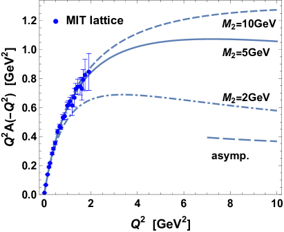
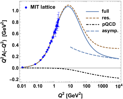
Figure 2: Left: The tensor gravitational form factor of the pion multiplied by $Q^{2}$, in the model with two resonances and pQCD for $M_{1}=m_{f_{2}}=1.275$ GeV and several values of $M_{2}$ indicated in the figure. Right: Anatomy of $Q^{2}A(Q^{2})$ for $M_{1}=m_{f_{2}}=1.275$ GeV and $M_{2}=5$ GeV. Full result (solid), the resonance contribution (dashed), the pQCD contribution (dot-dashed) of Eq. (46), and the asymptotic limit of Eq. (42) (long dash). The lattice MIT data are from [11].

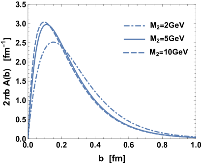
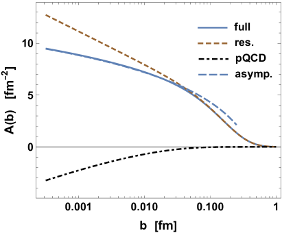
Figure 3: Left: Tensor gravitational transverse density of the pion in the model with two resonances and pQCD, for $M_{1}=m_{f_{2}}=1.275$ GeV and several values of $M_{2}$. Right: Anatomy of $A(b)$ for $M_{1}=m_{f_{2}}=1.275$ GeV and $M_{2}=5$ GeV. Full result (solid), the resonance contribution (dashed), the pQCD contribution (dot-dashed), and the asymptotic limit of Eq. (58) (long dash).

For $A$ we neglect the tiny NNLO $\chi$PT contribution, but retain the LO pQCD piece. The results shown in Fig. 2 are for $M_{1}$ set to the PDG value of the $f_{2}(1275)$ meson and for several large values of $M_{2}$. The comparison with the MIT lattice QCD data [11] in the left panel shows that values of $M_{2}$ from $\sim 5$ GeV upwards are admissible, whereas $M_{2}=2$ GeV is visibly too low. The values of the couplings for $M_{2}=5$ GeV are $a_{1}=1.06$ and $a_{2}=-0.056$, while $c_{\rm nr}=-0.004$, in satisfaction of the charge sum rule. Of course, the coupling of the second resonance is negative, and its contribution to the asymptotic sum rule is large due to the large value of $M_{2}>M_{1}$. The anatomy of $A$ is shown in the right panel of Fig. 2. We note a very slow approach to the asymptotic pQCD limit, which reflects the large value of $M_{2}$ required by the data. Asymptotically, the $1/Q^{2}$ tail contribution from the resonances is exactly canceled by the pQCD contribution of Eq. (46) via sum rule (36), leaving the proper pQCD asymptotic tail of Eq. (42). In Fig. 3 we present the corresponding transverse density (multiplied with $2\pi b$). We note that it satisfies the positivity condition $A(b)>0$ (cf. Sec. 3.4). The left panel shows the comparison of several values of $M_{2}$, whereas the right panel shows the various components of $A(b)$, with the cancelation at low $b$ as discussed around Eq. (58).

6.4   $\Theta$

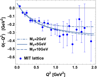
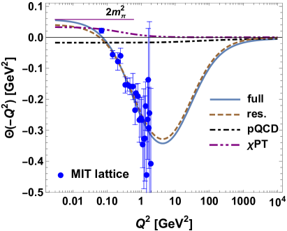
Figure 4: Left: The scalar gravitational form factor of the pion in the model with two resonances, pQCD, and $\chi$PT for $M_{1}=m_{\sigma}=800$ MeV and several values of $M_{2}$. Right: Anatomy of $\Theta(Q^{2})$ for $M_{1}=m_{\sigma}=800$ MeV and $M_{2}=5$ GeV. Full result (solid), the resonance contribution (dashed), the pQCD contribution (dot-dashed) of Eq. (46), the $\chi$PT contribution (dot-dot-dashed), and the asymptotic limit of Eq. (42) (long dash). The lattice MIT data are from [11].

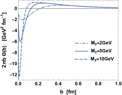
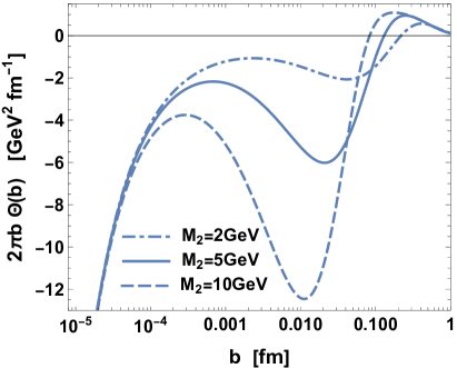
Figure 5: Left: Scalar gravitational transverse density of the pion in the model with two resonances and pQCD, for $M_{1}=m_{\sigma}=800$ MeV and several values of $M_{2}$. Right: Same as the right panel but for $b$ in the logarithmic scale.

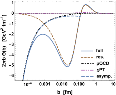
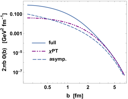
Figure 6: Left: Anatomy of $2\pi b\,\Theta(b)$ for $M_{1}=m_{\sigma}=800$ MeV and $M_{2}=5$ GeV. The asymptotics at low $b$ is from Eq. (60). Right: Same as the right panel but with the focus on large $b$ and asymptotics from Eq. (65).

The results for the scalar gravitational form factor in the model with two resonances are displayed in Fig. 4. We use an effective sigma meson of mass $m_{\sigma}=800$ MeV and several values of $M_{2}$. The slope is set to $S=0.9$ [36, 37]. As is apparent from the plot in the left panel, the lattice data are yet not accurate enough to discriminate between different values of $M_{2}$, with values from $\sim 2$ GeV upwards admissible. The right panel shows the anatomy of $\Theta(-Q^{2})$. In Fig. 5 we show $2\pi b\,\Theta(b)$. We note a singularity at $b\to 0$, the crossing of zero at $b\sim 0.2$ fm, and a non-monotonic behavior a lower values of $b$. The anatomy is displayed in Fig. 6. We note that in the range $\sim 0.01-1$ fm the resonance contribution dominates.

6.5 Transverse pressure

Finally, we look at one of the mechanistic properties of the pion, namely, the transverse pressure, obtained from the two gravitational transverse densities. From Eq. (16), by contracting with $\delta_{ij}$ ($i,j=1,2$), one readily finds

$$2P^{+}p(b)=-\frac{1}{4}\int\frac{d^{2}q_{\perp}}{(2\pi)^{2}}e^{-iq_{\perp}\cdot b}q_{\perp}^{2}D(-q_{\perp}^{2})=$$

$$~~~~-\frac{1}{6}\int\frac{d^{2}q_{\perp}}{(2\pi)^{2}}e^{-iq_{\perp}\cdot b}\left[\Theta(-q_{\perp}^{2})-(2m_{\pi}^{2}+\tfrac{1}{2}\,q_{\perp}^{2})A(-q_{\perp}^{2})\right],$$ (76)

where Eq. (6) has been used. With the behavior of $\Theta(-q_{\perp}^{2})$ and $A(-q_{\perp}^{2})$ near 0 we find that $\int d^{2}b\,p(b)=0$. Also, $2P^{+}\int d^{2}b\,p(b)=\tfrac{1}{4}D(0)$, which is the transverse version of the relation given in [3]. From Eq. (76) and the $b$-representations of the form factors we find

$$2P^{+}p(b)=-\frac{1}{6}\Theta(b)+\frac{m_{\pi}^{2}}{3}A(b)-\frac{1}{12}A_{1}(b),$$ (77)

where

$$A_{1}(b)=-\int\frac{d^{2}q_{\perp}}{(2\pi)^{2}}e^{-iq_{\perp}\cdot b}q_{\perp}^{2}A(-q_{\perp}^{2})=\int\frac{d^{2}q_{\perp}}{(2\pi)^{2}}e^{-iq_{\perp}\cdot b}\times$$ (78)

$$~~~\frac{1}{\pi}\int_{4m_{\pi}^{2}}^{\infty}ds\left[\frac{s}{s+q_{\perp}^{2}}-1\right]{\rm Im}\,A(s)=\frac{1}{2\pi^{2}}\int_{4m_{\pi}^{2}}^{\infty}ds\,K_{0}(b\sqrt{s})\,s\,{\rm Im}\,A(s),$$

where the term with -1 in the square bracket (that would yield a singular contribution proportional to $\delta^{2}(b)$) cancels thanks to the asymptotic sum rule (36). Derivation as for Eq. (60) gives at low $b$ the singularity

$$A_{1}(b)=-\frac{196\pi f_{\pi}^{2}}{\beta_{0}}\frac{1}{b^{2}\ln^{2}\left(\frac{1}{b^{2}\Lambda^{2}}\right)}+\dots,$$ (79)

which is one power of the log stronger than the singularity in $\Theta(b)$ of Eq. (57). From here we can see that $p(b)$ tends to positive infinity in the $b\to 0$ limit,

$$2\pi p(b)=\frac{49\pi f_{\pi}^{2}}{3\beta_{0}}\frac{1}{b^{2}\ln^{2}\left(\frac{1}{b^{2}\Lambda^{2}}\right)}+{\cal O}[1/(b^{2}\ln^{3}b)]$$ (80)

On the other end, at $b\to\infty$ it approaches 0 from below, hence must change sign. This is in compliance with stability, where a positive pressure in the inner region is balanced with a negative pressure outside.

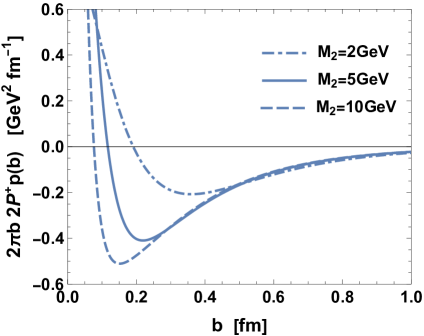
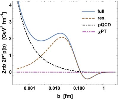
Figure 7: Left: Transverse pressure in the pion, $2\pi b\,2P^{+}p(b)$, in the model with two resonances per $A$ and $\Theta$, pQCD, and $\chi$PT. We take $m_{f_{2}}=1.275$ GeV, $m_{\sigma}=800$ MeV, and several values of $M_{2}$, same for both channels. Right: Anatomy of the transverse pressure for $M_{2}=5$ GeV.

The above statements concerning pressure arrival are general. We now pass to an illustration in the model used in the previous sections, with two resonances in each channel. The results are shown in Fig. 7. We note the dominance of the resonance contribution in the range $\sim 0.01-1$ fm, and a remarkable smallness of the $\chi$PT component, which nevertheless becomes dominant at large $b$ (above $\sim 3$ fm), as required by the limits (63).

7 Conclusions

Table 2: Summary of the gravitational properties of the pion.

quantity	low limit	intermediate range	high limit
${\rm Im}\,F(s),{\rm Im}\,A(s)$	$+$ Eq. (54)	changes sign	$-$ Eq. (44
${\rm Im}\,\Theta(s)$	$+$ Eq. (54)	changes sign	$-$ Eq. (45
$F(-Q^{2}),A(-Q^{2})$	$+$ $1$		$-$ Eq. (42
$\Theta(-Q^{2})$	$+$ $2m_{\pi}^{2}$	changes sign	$-$ Eq. (43
$F(b),A(b)$	$+$ Eq. (59)	positive definite	$+$ Eq. (63
$\Theta(b)$	$-$ Eq. (60)	changes sign	$+$ Eq. (63

In this contribution we have reviewed some general features of the gravitational form factors and the related transverse densities of the pion. We have used analyticity and the available information from $\pi-\pi$ scattering and pQCD to draw general conclusions on the behavior of these quantities. In particular, the scalar gravitational transverse density (related to the trace anomaly) must change sign as a function of the transverse coordinate $b$. On the other hand, the tensor gravitational transverse density (similarly to the electromagnetic charge case) is positive definite for all values of $b$, as deduced in the light-front quantization framework in the $A^{+}=0$ gauge. This positivity feature allows for a probabilistic interpretation.

The basic properties of the spectral densities, form factors for space-like momenta, and the transverse densities are collected in Table 2, with references to the explicit formulas in the text. The signs of the low- and high values of the arguments are indicated. For the spectral densities, the “low” limit means the behavior right from the $2\pi$ production threshold, while “high” means the asymptotic limit. For the other cases “low” means at zero.

We have also discussed the implications of the recent MIT lattice QCD analysis of the pion GFFs in the space-like region for $0<Q^{2}<2~{\rm GeV}^{2}$, which roughly maps into the $b>0.1~{\rm fm}$ region, and show that the data can be well described within the meson dominance approach. While a single resonance per channel suffices, to satisfy the sum rules following from the short-distance constraints of pQCD (the large-$Q^{2}$ behavior), we have added the needed negative contribution to the spectral densities in the form of a delta function and argued it has to appear at sufficiently high $s$, at least a few GeV², not to spoil the agreement with the lattice data.

We are grateful to the authors of Ref. [11] for providing us the data used in the figures. ERA was supported by Spanish MINECO and European FEDER funds grant and Project No. PID2023-147072NB-I00 funded by MCIN/AEI/10.13039/501100011033, and by the Junta de Andalucía grant FQM-225.

References

- Polyakov and Weiss [1999] M. V. Polyakov and C. Weiss, Phys. Rev. D 60, 114017 (1999), arXiv:hep-ph/9902451 .
- Polyakov [2003] M. V. Polyakov, Phys. Lett. B 555, 57 (2003), arXiv:hep-ph/0210165 .
- Polyakov and Schweitzer [2018] M. V. Polyakov and P. Schweitzer, Int. J. Mod. Phys. A 33, 1830025 (2018), arXiv:1805.06596 [hep-ph] .
- Carruthers [1971] P. Carruthers, Phys. Rept. 1, 1 (1971).
- Sharp and Wagner [1963] D. H. Sharp and W. G. Wagner, Physical Review 131, 2226 (1963).
- Pagels [1966] H. Pagels, Phys. Rev. 144, 1250 (1966).
- Raman [1971] K. Raman, Phys. Rev. D 4, 476 (1971).
- Truong and Willey [1989] T. N. Truong and R. S. Willey, Phys. Rev. D 40, 3635 (1989).
- Gasser and Meissner [1991] J. Gasser and U. G. Meissner, Nucl. Phys. B 357, 90 (1991).
- Donoghue and Leutwyler [1991] J. F. Donoghue and H. Leutwyler, Z. Phys. C 52, 343 (1991).
- Hackett et al. [2023] D. C. Hackett, P. R. Oare, D. A. Pefkou, and P. E. Shanahan, Phys. Rev. D 108, 114504 (2023), arXiv:2307.11707 [hep-lat] .
- Pefkou [2023] D. A. Pefkou, Gravitational form factors of hadrons from lattice QCD, Ph.D. thesis, MIT (2023).
- Brommel [2007] D. Brommel, Pion Structure from the Lattice, Ph.D. thesis, Regensburg U. (2007).
- Brömmel et al. [2008] D. Brömmel et al. (QCDSF, UKQCD), Phys. Rev. Lett. 101, 122001 (2008), arXiv:0708.2249 [hep-lat] .
- Delmar et al. [2024] J. Delmar, C. Alexandrou, S. Bacchio, I. Cloët, M. Constantinou, and G. Koutsou, in 40th International Symposium on Lattice Field Theory (2024) arXiv:2401.04080 [hep-lat] .
- Shanahan and Detmold [2019] P. E. Shanahan and W. Detmold, Phys. Rev. D 99, 014511 (2019), arXiv:1810.04626 [hep-lat] .
- Wang et al. [2024a] B. Wang, F. He, G. Wang, T. Draper, J. Liang, K.-F. Liu, and Y.-B. Yang (QCD), Phys. Rev. D 109, 094504 (2024a), arXiv:2401.05496 [hep-lat] .
- Masuda et al. [2016] M. Masuda et al. (Belle), Phys. Rev. D 93, 032003 (2016), arXiv:1508.06757 [hep-ex] .
- Kumano et al. [2018] S. Kumano, Q.-T. Song, and O. V. Teryaev, Phys. Rev. D 97, 014020 (2018), arXiv:1711.08088 [hep-ph] .
- Broniowski et al. [2008] W. Broniowski, E. Ruiz Arriola, and K. Golec-Biernat, Phys. Rev. D 77, 034023 (2008), arXiv:0712.1012 [hep-ph] .
- Broniowski and Ruiz Arriola [2008] W. Broniowski and E. Ruiz Arriola, Phys. Rev. D 78, 094011 (2008), arXiv:0809.1744 [hep-ph] .
- Frederico et al. [2009] T. Frederico, E. Pace, B. Pasquini, and G. Salme, Phys. Rev. D 80, 054021 (2009), arXiv:0907.5566 [hep-ph] .
- Masjuan et al. [2013] P. Masjuan, E. Ruiz Arriola, and W. Broniowski, Phys. Rev. D 87, 014005 (2013), arXiv:1210.0760 [hep-ph] .
- Fanelli et al. [2016] C. Fanelli, E. Pace, G. Romanelli, G. Salme, and M. Salmistraro, Eur. Phys. J. C 76, 253 (2016), arXiv:1603.04598 [hep-ph] .
- Freese and Cloët [2019] A. Freese and I. C. Cloët, Phys. Rev. C 100, 015201 (2019), [Erratum: Phys.Rev.C 105, 059901 (2022)], arXiv:1903.09222 [nucl-th] .
- Krutov and Troitsky [2021] A. F. Krutov and V. E. Troitsky, Phys. Rev. D 103, 014029 (2021), arXiv:2010.11640 [hep-ph] .
- Xing et al. [2023] Z. Xing, M. Ding, and L. Chang, Phys. Rev. D 107, L031502 (2023), arXiv:2211.06635 [hep-ph] .
- Xu et al. [2024] Y.-Z. Xu, M. Ding, K. Raya, C. D. Roberts, J. Rodríguez-Quintero, and S. M. Schmidt, Eur. Phys. J. C 84, 191 (2024), arXiv:2311.14832 [hep-ph] .
- Li and Vary [2024] Y. Li and J. P. Vary, Phys. Rev. D 109, L051501 (2024), arXiv:2312.02543 [hep-th] .
- Liu et al. [2024a] W.-Y. Liu, E. Shuryak, C. Weiss, and I. Zahed, Phys. Rev. D 110, 054021 (2024a), arXiv:2405.14026 [hep-ph] .
- Liu et al. [2024b] W.-Y. Liu, E. Shuryak, and I. Zahed, Phys. Rev. D 110, 054022 (2024b), arXiv:2405.16269 [hep-ph] .
- Wang et al. [2024b] X. Wang, Z. Xing, M. Ding, K. Raya, and L. Chang, (2024b), arXiv:2406.09644 [hep-ph] .
- Sultan et al. [2024] M. A. Sultan, Z. Xing, K. Raya, A. Bashir, and L. Chang, Phys. Rev. D 110, 054034 (2024), arXiv:2407.10437 [hep-ph] .
- Fujii et al. [2024] D. Fujii, A. Iwanaka, and M. Tanaka, (2024), arXiv:2407.21113 [hep-ph] .
- Krutov and Troitsky [2024] A. F. Krutov and V. E. Troitsky, (2024), arXiv:2410.17570 [hep-ph] .
- Broniowski and Ruiz Arriola [2024] W. Broniowski and E. Ruiz Arriola, Phys. Lett. B 859, 139138 (2024), arXiv:2405.07815 [hep-ph] .
- Ruiz Arriola and Broniowski [2024] E. Ruiz Arriola and W. Broniowski (2024) arXiv:2411.10354 [hep-ph] .
- Cao et al. [2024] X.-H. Cao, F.-K. Guo, Q.-Z. Li, and D.-L. Yao, (2024), arXiv:2411.13398 [hep-ph] .
- Tong et al. [2021] X.-B. Tong, J.-P. Ma, and F. Yuan, Phys. Lett. B 823, 136751 (2021), arXiv:2101.02395 [hep-ph] .
- Tong et al. [2022] X.-B. Tong, J.-P. Ma, and F. Yuan, JHEP 10, 046 (2022), arXiv:2203.13493 [hep-ph] .
- Pokorski [2005] S. Pokorski, Gauge field theories (Cambridge University Press, 2005).
- Belitsky and Radyushkin [2005] A. V. Belitsky and A. V. Radyushkin, Phys. Rept. 418, 1 (2005), arXiv:hep-ph/0504030 .
- Soper [1977] D. E. Soper, Phys. Rev. D 15, 1141 (1977).
- Burkardt [2000] M. Burkardt, Phys. Rev. D 62, 071503 (2000), [Erratum: Phys.Rev.D 66, 119903 (2002)], arXiv:hep-ph/0005108 .
- Diehl [2002] M. Diehl, Eur. Phys. J. C 25, 223 (2002), [Erratum: Eur.Phys.J.C 31, 277–278 (2003)], arXiv:hep-ph/0205208 .
- Burkardt [2003] M. Burkardt, Int. J. Mod. Phys. A 18, 173 (2003), arXiv:hep-ph/0207047 .
- Miller [2010] G. A. Miller, Ann. Rev. Nucl. Part. Sci. 60, 1 (2010), arXiv:1002.0355 [nucl-th] .
- Freese and Miller [2023] A. Freese and G. A. Miller, Phys. Rev. D 108, 034008 (2023), arXiv:2210.03807 [hep-ph] .
- Pobylitsa [2002] P. V. Pobylitsa, Phys. Rev. D66, 094002 (2002), hep-ph/0204337 .
- Freese and Miller [2022] A. Freese and G. A. Miller, Phys. Rev. D 105, 014003 (2022), arXiv:2108.03301 [hep-ph] .
- Panteleeva and Polyakov [2021] J. Y. Panteleeva and M. V. Polyakov, Phys. Rev. D 104, 014008 (2021), arXiv:2102.10902 [hep-ph] .
- Donoghue and Na [1997] J. F. Donoghue and E. S. Na, Phys. Rev. D 56, 7073 (1997), arXiv:hep-ph/9611418 .
- Gasser and Leutwyler [1984] J. Gasser and H. Leutwyler, Annals Phys. 158, 142 (1984).
- Miller et al. [2011a] G. A. Miller, M. Strikman, and C. Weiss, Phys. Rev. D 83, 013006 (2011a), arXiv:1011.1472 [hep-ph] .
- Miller et al. [2011b] G. A. Miller, M. Strikman, and C. Weiss, Phys. Rev. C 84, 045205 (2011b), arXiv:1105.6364 [hep-ph] .
- Ruiz Arriola and Sanchez-Puertas [2024] E. Ruiz Arriola and P. Sanchez-Puertas, Phys. Rev. D 110, 054003 (2024), arXiv:2403.07121 [hep-ph] .
- Sanchez-Puertas and Ruiz Arriola [2024] P. Sanchez-Puertas and E. Ruiz Arriola, in 10th International Conference on Quarks and Nuclear Physics (2024) arXiv:2410.17804 [hep-ph] .
- Ruiz Arriola et al. [2024] E. Ruiz Arriola, P. Sanchez-Puertas, and C. Weiss, Work in preparation (2024).
- Miller [2009] G. A. Miller, Phys. Rev. C 79, 055204 (2009), arXiv:0901.1117 [nucl-th] .
- Colangelo et al. [2001] G. Colangelo, J. Gasser, and H. Leutwyler, Nucl. Phys. B 603, 125 (2001), arXiv:hep-ph/0103088 .
- Garcia-Martin et al. [2011] R. Garcia-Martin, R. Kaminski, J. R. Pelaez, J. Ruiz de Elvira, and F. J. Yndurain, Phys. Rev. D 83, 074004 (2011), arXiv:1102.2183 [hep-ph] .
- Ruiz Arriola and Broniowski [2008] E. Ruiz Arriola and W. Broniowski, Phys. Rev. D 78, 034031 (2008), arXiv:0807.3488 [hep-ph] .