Exponential and algebraic double-soliton solutions of the massive Thirring model

Abstract.

The newly discovered exponential and algebraic double-soliton solutions of the massive Thirring model in laboratory coordinates are placed in the context of the inverse scattering transform. We show that the exponential double-solitons correspond to double isolated eigenvalues in the Lax spectrum, whereas the algebraic double-solitons correspond to double embedded eigenvalues on the imaginary axis, where the continuous spectrum resides. This resolves the long-standing conjecture that multiple embedded eigenvalues may exist in the spectral problem associated with the massive Thirring model. To obtain the exponential double-solitons, we solve the Riemann–Hilbert problem with the reflectionless potential in the case of a quadruplet of double poles in each quadrant of the complex plane. To obtain the algebraic double-solitons, we consider the singular limit where the quadruplet of double poles degenerates into a symmetric pair of double embedded poles on the imaginary axis.

1. Introduction

We address the massive Thirring model (MTM) in laboratory coordinates, which can be written in the following normalized form

$$\begin{split}i(u_{t}+u_{x})+v+|v|^{2}u=0,\\ i(v_{t}-v_{x})+u+|u|^{2}v=0,\end{split}$$ (1.1)

where $u=u(x,t)$ and $v=v(x,t)$ are complex functions of real variables $x$ and $t$. The MTM was introduced in [25] in the context of quantum field theory as a relativistically invariant nonlinear Dirac equation in one spatial dimension. It was found in [20] (see also [14, 16, 21]) that the MTM is a commutativity condition for a Lax pair of linear equations, hence it is completely integrable by the inverse scattering transform (IST) method. The Lax pair of linear equations for the MTM is given by

$$\partial_{x}\psi=L(u,v,\zeta)\psi,\quad\partial_{t}\psi=A(u,v,\zeta)\psi,$$ (1.2)

where $\zeta\in\mathbb{C}$ is the spectral parameter, $\psi=\psi(x,t)\in\mathbb{C}^{2}$ is the wave function, and the $2$-by-$2$ matrices $L(u,v,\zeta)$ and $A(u,v,\zeta)$ are given by

$$L=\frac{i}{4}\left(|u|^{2}-|v|^{2}\right)\sigma_{3}-\frac{i}{2}\zeta\left(\begin{array}[]{cc}0&\bar{v}\\ v&0\\ \end{array}\right)+\frac{i}{2\zeta}\left(\begin{array}[]{cc}0&\bar{u}\\ u&0\\ \end{array}\right)+\frac{i}{4}\left(\zeta^{2}-\zeta^{-2}\right)\sigma_{3}$$

and

$$A=-\frac{i}{4}\left(|u|^{2}+|v|^{2}\right)\sigma_{3}-\frac{i}{2}\zeta\left(\begin{array}[]{cc}0&\bar{v}\\ v&0\\ \end{array}\right)-\frac{i}{2\zeta}\left(\begin{array}[]{cc}0&\bar{u}\\ u&0\\ \end{array}\right)+\frac{i}{4}\left(\zeta^{2}+\zeta^{-2}\right)\sigma_{3}.$$

Here the bar stands for the complex conjugation and $\sigma_{3}={\rm diag}(1,-1)$ is the third Pauli’s matrix. The compatibility condition $\partial_{t}\partial_{x}\psi=\partial_{x}\partial_{t}\psi$ in the linear system (1.2) coincides with the MTM system (1.1).

The IST method based on the Riemann–Hilbert (RH) problem has been applied for the Lax pair (1.2) in the recent works [23] and [9, 18] (see also earlier works [26] and [17]). The IST method is used to obtain global solutions and to study the long-time dynamics of the MTM system (1.1) for the initial-value problem with the initial data $(u,v)|_{t=0}=(u_{0},v_{0})$ decaying to zero at infinity. The decay condition on $(u_{0},v_{0})$ is required to be sufficiently fast so that the functions and their first and second derivatives are square integrable with the weight $\sqrt{1+x^{2}}$ [9]. Exponential solitons satisfy this requirement and each soliton corresponds to a quadruplet of simple poles of the RH problem in each quadrant of the complex plane, or equivalently to simple isolated eigenvalues in the Lax spectrum of the linear system (1.2). However, algebraic solitons decay as $(u,v)=\mathcal{O}(|x|^{-1})$ as $|x|\to\infty$ and hence they are not included in the IST method. Each algebraic soliton corresponds to a simple embedded eigenvalue in the Lax spectrum located on the imaginary axis (no embedded eigenvalues exist on the real axis).

The algebraic solitons in the MTM were studied in [15], where the perturbation theory for embedded eigenvalues in the Lax spectrum of the linear system (1.2) was developed. It was shown in [15, Proposition 7.1] that a pair of simple embedded eigenvalues on the imaginary axis is structurally unstable and moves into a quadruplet of simple isolated eigenvalues in each quadrant of the complex plane under a generic perturbation of the initial data. A possibility of embedded eigenvalues of a higher algebraic multiplicity was also suggested in [15, Lemma 6.4] with some precise conditions on the spatial decay of eigenvectors and generalized eigenvectors at infinity. Such embedded eigenvalues of higher algebraic multiplicity generally correspond to rational solutions of the MTM describing algebraic multi-solitons. However, the existence of such rational solutions has not been established in the literature up to very recently, despite many works on rational solutions in integrable systems (see, e.g., [6, 7, 10, 22, 29, 30, 31]).

Rational solutions of the MTM were constructed on the constant nonzero background in [5, 12, 32]. They are relevant to dynamics of rogue waves on the modulationally unstable background but do not describe the dynamics of algebraic solitons at the zero background. It was only recently shown in [8] (based on the Hirota’s bilinear method developed in [4]) that the algebraic double-solitons exist as the exact solutions of the MTM suggesting the existence of the higher-order algebraic solitons in a hierarchy of rational solutions to the MTM. Within the bilinear method, it was not shown in [8] that the algebraic double-solitons correspond to the double embedded eigenvalues in the Lax spectrum predicted in [15].

The main motivation for our work is to use the RH problem and to obtain the algebraic double-solitons of the MTM system (1.1) associated with the double embedded eigenvalues in the Lax spectrum of the linear system (1.2). To derive this result, we construct the exponential double-solitons associated with a quadruplet of double isolated eigenvalues in each quadrant of the complex plane and take the singular limit when the quadruplet of double isolated eigenvalues transforms into a symmetric pair of double embedded eigenvalues on the imaginary axis.

The study of double eigenvalues has started with the pioneering work [34], where it was shown that the double eigenvalues of the associated spectral problem give the exponential double-solitons describing the slow (logarithmic in time) dynamics of two identical solitons of the focusing nonlinear Schrödinger (NLS) equation. Properties of such exponential double-solitons were recently studied in nonintegrable versions of the NLS equation in [19]. The exponential double-solitons on the nonzero constant background were constructed in [24] after the development in the IST methods on the nonzero background in [3].

The double-soliton solutions in the closely related derivative NLS equation were constructed by using the Darboux transformations in [28, 33] and [11]. It was understood in [33] that the algebraic double-solitons arise from the exponential double-solitons in the singular limit, for which the modified Darboux transformations have been developed in [11]. The IST method was also employed in the context of the derivative NLS equation to construct the exponential double-solitons from the double poles of the RH problem in [27, 35, 36, 37]. Although both the derivative NLS equation and the MTM system in characteristic coordinates are related to the same spectral problem [13, 14], the computational details for the MTM system in laboratory coordinates are different and technically more complicated. We close this gap in the literature by presenting the exponential double-solitons of the MTM system (1.1) for the double isolated eigenvalues of the linear system (1.2). The main application of this result is to obtain the algebraic double-solitons and the double embedded eigenvalues in the singular limit, where the RH problem cannot be used.

For the spectral problem associated with the focusing NLS equation on a nonzero background, it was understood in [1] how to modify the RH problem for the simple and multiple embedded eigenvalues at the end points of the continuous spectrum in order to construct the rogue waves [2]. This modification of the RH problem has not been developed so far for the spectral problem associated with the derivative NLS equation and the MTM system on the zero background. It is still unclear how the simple or multiple embedded eigenvalues can be constructed in the RH problem directly. We hope that our work will motivate further study of the associated spectral problems with embedded eigenvalues.

This paper is organized as follows. Section 2 introduces the RH problem for the MTM and formulates the main results. The exponential double-solitons are constructed in Section 3 from the isolated double-pole solutions of the RH problem. The algebraic double-solitons are obtained in Section 4 by taking the singular limit to the embedded double-pole solutions of the RH problem. Appendix A reports similar computations for the exponential and algebraic single-solitons for convenience of readers. Appendix B reviews the construction of the exponential double-solitons in the MTM system by using the bilinear Hirota method.

2. RH problem for MTM and main results

Assume that $(u,v)\to(0,0)$ as $|x|\to\infty$ fast enough, see Lemmas 2.1 and 2.2 below for precise requirements on $(u,v)$. We define the matrix Jost functions for the linear system (1.2) from the boundary conditions:

$$\psi^{(\pm)}(\zeta,x,t)\to\left(\begin{matrix}e^{\frac{i}{4}\left(\zeta^{2}-\zeta^{-2}\right)x+\frac{i}{4}\left(\zeta^{2}+\zeta^{-2}\right)t}&0\\ 0&e^{-\frac{i}{4}\left(\zeta^{2}-\zeta^{-2}\right)x-\frac{i}{4}\left(\zeta^{2}+\zeta^{-2}\right)t}\end{matrix}\right)\quad\mbox{\rm as}\quad x\to\pm\infty.$$ (2.1)

For simplicity of notations, we will drop the dependence of $\psi^{(\pm)}$ on $(x,t)$. Since the Jost functions $\psi^{\pm}(\zeta)$ represent the fundamental matrix solutions of the linear sytem (1.2), they are related to each other by the scattering relations introduced for $\zeta\in(\mathbb{R}\cup i\mathbb{R})\backslash\{0\}$ as

$$\psi^{(-)}(\zeta)=\psi^{(+)}(\zeta)\left(\begin{array}[]{cc}\overline{a}(\zeta)&b(\zeta)\\ -\overline{b}(\zeta)&a(\zeta)\\ \end{array}\right),$$ (2.4)

where the symmetry of scattering coefficients $a(\zeta)$ and $b(\zeta)$ follows from the symmetry of matrix Jost functions:

$$\psi^{(\pm)}(\zeta)=\left(\begin{array}[]{cc}0&-1\\ 1&0\\ \end{array}\right)\overline{\psi}^{(\pm)}(\zeta)\left(\begin{array}[]{cc}0&1\\ -1&0\\ \end{array}\right).$$ (2.9)

As is explained in [23], the linear system (1.2) can be folded to the squared spectral parameter $\lambda:=\zeta^{2}$ in two different ways, one is suitable near $\zeta=0$ and the other one is suitable near $\zeta=\infty$. Following [9], we will only consider the second transformation, from which we will define the Riemann-Hilbert (RH) problem and solve it for the exponential double-solitons, see Theorem 2.1 below.

Hence we introduce the modified Jost functions as

$$\left\{\begin{array}[]{l}n_{1}^{(\pm)}(\lambda):=T(v,\zeta)\psi_{1}^{(\pm)}(\zeta)e^{-\frac{i}{4}\left(\zeta^{2}-\zeta^{-2}\right)x-\frac{i}{4}\left(\zeta^{2}+\zeta^{-2}\right)t},\\ n_{2}^{(\pm)}(\lambda):=\zeta^{-1}T(v,\zeta)\psi_{2}^{(\pm)}(\zeta)e^{\frac{i}{4}\left(\zeta^{2}-\zeta^{-2}\right)x+\frac{i}{4}\left(\zeta^{2}+\zeta^{-2}\right)t},\end{array}\right.$$ (2.12)

where the subscripts indicate the columns of the $2$-by-$2$ matrices and the transformation matrix is given by

$$T(v,\zeta):=\left(\begin{array}[]{cc}1&0\\ v&\zeta\\ \end{array}\right).$$

It follows from (2.1) that the modified Jost functions satisfy

$$n_{1}^{(\pm)}(\lambda)\to e_{1}:=\left(\begin{matrix}1\\ 0\end{matrix}\right),\quad n_{2}^{(\pm)}(\lambda)\to e_{2}:=\left(\begin{matrix}0\\ 1\end{matrix}\right)\quad\mbox{\rm as}\quad x\to\pm\infty.$$

Moreover, $n_{1,2}^{(\pm)}(\lambda)$ satisfy the integral equations, from which the following properties were proven in [23, Lemmas 3–5].

Lemma 2.1.

Let $(u,v)\in L^{1}(\mathbb{R})\cap L^{\infty}(\mathbb{R})$ and $(u_{x},v_{x})\in L^{1}(\mathbb{R})$. For every $\lambda\in\mathbb{R}\setminus\{0\}$, there exists unique bounded Jost functions $n_{1}^{(\pm)}(\lambda)$ and $n_{2}^{(\pm)}(\lambda)$. For every $x\in\mathbb{R}$, $n_{1}^{(\pm)}$ and $n_{2}^{(\pm)}$ are continued analytically in $\mathbb{C}^{\pm}$ and satisfy the following limits as $|\lambda|\to\infty$ and $\lambda\to 0$ along a contour in the domains of their analyticity:

$$\lim_{|\lambda|\to\infty}\frac{n_{1}^{(\pm)}(\lambda)}{n^{\pm\infty}_{1}}=e_{1},\quad\lim_{|\lambda|\to\infty}\frac{n_{2}^{(\pm)}(\lambda)}{n^{\pm\infty}_{2}}=e_{2},$$ (2.13)

and

$$\lim_{\lambda\to 0}\left[n^{\pm\infty}_{1}n_{1}^{(\pm)}(\lambda)\right]=e_{1}+ve_{2},\quad\lim_{\lambda\to 0}\left[n^{\pm\infty}_{2}n_{2}^{(\pm)}(\lambda)\right]=\bar{u}e_{1}+(1+\bar{u}v)e_{2},$$ (2.14)

where

$$n^{\pm\infty}_{1}:=e^{\frac{i}{4}\int_{\pm\infty}^{x}(|u|^{2}+|v|^{2})dy},\quad n^{\pm\infty}_{2}:=e^{-\frac{i}{4}\int_{\pm\infty}^{x}(|u|^{2}+|v|^{2})dy}.$$

Recall that $\lambda:=\zeta^{2}$ and that $\lambda\in\mathbb{R}$ for $\zeta\in(\mathbb{R}\cup i\mathbb{R})$. Hence we define new scattering coefficients for $\lambda\in\mathbb{R}\backslash\{0\}$ as

$$\alpha(\lambda):=a(\zeta),\quad\beta_{+}(\lambda):=\zeta b(\zeta),\quad\beta_{-}(\lambda):=\zeta^{-1}b(\zeta).$$

After the folding transformation (2.12), the scattering relations (2.4) are modified as follows

$$n^{(-)}(\lambda)=n^{(+)}(\lambda)\left(\begin{array}[]{cc}\overline{\alpha}(\lambda)&\beta_{-}(\lambda)e^{2i\theta(\lambda)}\\ -\overline{\beta}_{+}(\lambda)e^{-2i\theta(\lambda)}&\alpha(\lambda)\\ \end{array}\right),$$ (2.17)

where

$$\theta(\lambda):=\frac{1}{4}(\lambda-\lambda^{-1})x+\frac{1}{4}(\lambda+\lambda^{-1})t.$$ (2.18)

The following lemma was proven in [23, Lemma 6].

Lemma 2.2.

Let $(u,v)\in L^{1}(\mathbb{R})\cap L^{\infty}(\mathbb{R})$ and $(u_{x},v_{x})\in L^{1}(\mathbb{R})$. Then, $\alpha$ is continued analytically into $\mathbb{C}^{+}$ with the following limits in $\mathbb{C}^{+}$:

$$\lim_{|\lambda|\to\infty}\alpha(\lambda)=e^{-\frac{i}{4}\int_{\mathbb{R}}(|u|^{2}+|v|^{2})dy}$$ (2.19)

and

$$\lim_{\lambda\to 0}\alpha(\lambda)=e^{\frac{i}{4}\int_{\mathbb{R}}(|u|^{2}+|v|^{2})dy},$$ (2.20)

whereas $\beta_{\pm}$ are not continued analytically outside $\mathbb{R}$ and satisfy the limits

$$\lim_{|\lambda|\to\infty}\beta_{\pm}(\lambda)=\lim_{\lambda\to 0}\beta_{\pm}(\lambda)=0.$$

The RH problem for the modified Jost functions $n^{(\pm)}(\lambda)$ is constructed as follows. We first define the sectionally meromorphic matrix $P(\lambda)\in\mathbb{C}^{2\times 2}$ by

$$P(\lambda):=\left\{\begin{aligned} &\left(n^{(+)}_{1}(\lambda),\frac{n^{(-)}_{2}(\lambda)}{\alpha(\lambda)}\right),\quad\lambda\in\mathbb{C}^{+},\\ &\left(\frac{n^{(-)}_{1}(\lambda)}{\bar{\alpha}(\lambda)},n^{(+)}_{2}(\lambda)\right),\quad\lambda\in\mathbb{C}^{-}.\end{aligned}\right.$$ (2.21)

By using (2.13) and (2.19), we obtain the following limits as $|\lambda|\to\infty$ in the domain of meromorphicity of $P(\lambda)$:

$$\lim_{|\lambda|\to\infty}P(\lambda)=\left(\begin{array}[]{cc}n^{+\infty}_{1}&0\\ 0&n^{+\infty}_{2}\\ \end{array}\right)=:P^{\infty},$$ (2.24)

where $\overline{P^{\infty}}=(P^{\infty})^{-1}$. We finally define $M(\lambda):=(P^{\infty})^{-1}P(\lambda)$ and formulate the normalized RH problem.

RH problem. Find a complex-valued function $M(\lambda)$ with the following properties: • $M(\lambda)$ is meromorphic in $\mathbb{C}\setminus\mathbb{R}$. • $M(\lambda)\to\mathbb{I}$ as $|\lambda|\to\infty$, where $\mathbb{I}$ is the $2$-by-$2$ identity matrix. • $M_{+}(\lambda)=M_{-}(\lambda)V(\lambda)$ for every $\lambda\in\mathbb{R}$, where $M_{\pm}(\lambda):=\lim\limits_{{\rm Im}(\lambda)\to\pm 0}M(\lambda)$ and $\displaystyle V(\lambda):=\left(\begin{array}[]{cc}1&-r_{-}(\lambda)e^{2i\theta(\lambda)}\\ -\overline{r}_{+}(\lambda)e^{-2i\theta(\lambda)}&1+\overline{r}_{+}(\lambda)r_{-}(\lambda)\end{array}\right),\quad r_{\pm}(\lambda):=\frac{\beta_{\pm}(\lambda)}{\alpha(\lambda)}.$

It follows from (2.14) and (2.20) (see also [9, Proposition 2.24]) that the potentials $(u,v)$ for solutions of the MTM system (1.1) can be recovered from solutions of the RH problem by using the following asymptotic limits taken in the domains of meromorphicity of $M(\lambda)$:

$$u=\lim_{\lambda\to 0}\overline{M}_{12}(\lambda),\quad v=\lim_{\lambda\to 0}M_{21}(\lambda).$$ (2.25)

Solvability of the RH problem under some conditions of the reflection coefficients $r_{\pm}(\lambda)$ was studied in [9, 23]. In this work, we consider the reflectionless case $r_{\pm}(\lambda)\equiv 0$ for $\lambda\in\mathbb{R}$ in the particular case when $\alpha(\lambda)$ admits a double pole at $\lambda_{0}\in\mathbb{C}^{+}$.

It is well-known (see, e.g., [9, 18]) that a simple pole of $\alpha(\lambda)$ leads to a single-soliton solution. For completeness, we give details of the RH problem with a simple pole in Appendix A. To simplify the presentation of soliton solutions, we should use the basic symmetries of the MTM system. In particular, the relativistically invariant MTM system (1.1) admits the Lorentz symmetry

$$\left[\begin{matrix}u(x,t)\\ v(x,t)\end{matrix}\right]\;\;\mapsto\;\;\left[\begin{matrix}\left(\frac{1-c}{1+c}\right)^{1/4}u\left(\frac{x+ct}{\sqrt{1-c^{2}}},\frac{t+cx}{\sqrt{1-c^{2}}}\right)\\ \left(\frac{1+c}{1-c}\right)^{1/4}v\left(\frac{x+ct}{\sqrt{1-c^{2}}},\frac{t+cx}{\sqrt{1-c^{2}}}\right)\end{matrix}\right],\qquad c\in(-1,1).$$ (2.26)

In addition, it admits the translational and rotational symmetries

$$\left[\begin{matrix}u(x,t)\\ v(x,t)\end{matrix}\right]\quad\mapsto\quad\left[\begin{matrix}u(x+x_{0},t+t_{0})e^{\mathrm{i}\theta_{0}}\\ v(x+x_{0},t+t_{0})e^{\mathrm{i}\theta_{0}}\end{matrix}\right],\qquad x_{0},t_{0},\theta_{0}\in\mathbb{R}.$$ (2.27)

By using (2.26) and (2.27), the single-soliton solutions can be expressed in a short form:

$$\left\{\begin{array}[]{lr}u(x,t)=i(\sin\gamma){\rm sech}\left(x\sin\gamma-i\frac{\gamma}{2}\right)e^{-it\cos\gamma},\\ v(x,t)=-i(\sin\gamma){\rm sech}\left(x\sin\gamma+i\frac{\gamma}{2}\right)e^{-it\cos\gamma},\end{array}\right.$$ (2.28)

where $\gamma\in(0,\pi)$ is a free parameter. More general single-soliton solutions can be extended with speed parameter $c\in(-1,1)$ by using (2.26) and with two translational parameters $x_{0},t_{0}\in\mathbb{R}$ by using (2.27), where translation in $\theta_{0}$ is linearly dependent from translation in $t_{0}$.

The normalized single-soliton solution (2.28) corresponds to the simple pole of the RH problem at $\lambda_{0}=e^{i\gamma}\in\mathbb{C}^{+}$ with $\gamma\in(0,\pi)$, see Appendix A. The double-soliton solutions will also be constructed for $\lambda_{0}=e^{i\gamma}\in\mathbb{C}^{+}$. The following theorem gives the explicit representation of the double-soliton solutions. As we show in Appendix B, this representation coincides with the explicit formula obtained by the bilinear Hirota method developed in [4].

Theorem 2.1.

Let $\lambda_{0}=e^{i\gamma}$ with $\gamma\in(0,\pi)$ be a double pole of the RH problem. Then, the solution $(u,v)$ of the MTM system (1.1) obtained from (2.25) is given by

$$u=\frac{\bar{N}_{u}}{\overline{D(M)}},\quad v=\frac{N_{v}}{D(M)},$$ (2.29)

where

$$N_{u} =4i(\sin\gamma)^{2}e^{-x\sin\gamma+it\cos\gamma-\frac{i\gamma}{2}}\left((x-\tilde{x}_{0})\cos\gamma+i(t-\tilde{t}_{0})\sin\gamma+i\right.$$

$$\left.\quad-e^{-2x\sin\gamma-i\gamma}[2\cot\gamma+(x-\tilde{x}_{0})\cos\gamma-i(t-\tilde{t}_{0})\sin\gamma]\right),$$

$$N_{v} =4i(\sin\gamma)^{2}e^{-x\sin\gamma-it\cos\gamma-\frac{i\gamma}{2}}\left((x-\tilde{x}_{0})\cos\gamma-i(t-\tilde{t}_{0})\sin\gamma\right.$$

$$\left.\quad-e^{-2x\sin\gamma-i\gamma}[2\cot\gamma+(x-\tilde{x}_{0})\cos\gamma+i(t-\tilde{t}_{0})\sin\gamma+i]\right),$$

and

$$D(M) =1+e^{-4x\sin\gamma-2i\gamma}+2e^{-2x\sin\gamma-i\gamma}$$

$$\quad\times\left(1+2(\sin\gamma)^{2}\left[\cot\gamma+(x-\tilde{x}_{0})\cos\gamma+\frac{i}{2}\right]^{2}+2(\sin\gamma)^{4}\left[t-\tilde{t}_{0}+\frac{1}{2\sin\gamma}\right]^{2}\right),$$

where $\tilde{x}_{0},\tilde{t}_{0}\in\mathbb{R}$ are arbitrary parameters in addition to parameters $c\in(-1,1)$ and $x_{0},t_{0}\in\mathbb{R}$ obtained from the transformations (2.26) and (2.27).

Remark 2.2.

Parameter $\tilde{t}_{0}$ is trivially removed by using translational symmetries (2.27) with translations in $\theta_{0}$ and $t_{0}$. Hence, the double-soliton solutions of Theorem 2.1 only have two non-trivial parameters: $\gamma\in(0,\pi)$ and $\tilde{x}_{0}\in\mathbb{R}$.

Although the explicit form of double-soliton solutions in Theorem 2.1 can be obtained by algebraic methods such as Darboux transformations or the bilinear Hirota method, see Appendix B, the RH problem enables us to clarify the Lax spectrum of the double-soliton solutions. Based on the solution in Section 3, we prove that $\zeta_{0}:=\sqrt{\lambda_{0}}=e^{\frac{i}{2}\gamma}$ is a double eigenvalue of the linear system (1.2) with only one eigenvector $\psi_{0}\in H^{1}(\mathbb{R},\mathbb{C}^{2})$ and one generalized eigenvector $\psi_{1}\in H^{1}(\mathbb{R},\mathbb{C}^{2})$. The eigenvector and the generalized eigenvector satisfy the following linear equations:

$$\partial_{x}\psi_{0}=L(u,v,\zeta_{0})\psi_{0},\quad\partial_{t}\psi_{0}=A(u,v,\zeta_{0})\psi_{0}$$ (2.30)

and

$$\partial_{x}\psi_{1}=L(u,v,\zeta_{0})\psi_{1}+\partial_{\zeta}L(u,v,\zeta_{0})\psi_{0},\quad\partial_{t}\psi_{1}=A(u,v,\zeta_{0})\psi_{1}+\partial_{\zeta}A(u,v,\zeta_{0})\psi_{0},$$ (2.31)

where $(u,v)$ is given by (2.29) and $\zeta_{0}=e^{\frac{i\gamma}{2}}$.

The knowledge of eigenvectors and generalized eigenvectors in (2.30) and (2.31) is particularly important when the exponential double-soliton solution of Theorem 2.1 converges as $\gamma\to\pi$ to the algebraic double-soliton solution obtained in [8]. The following theorem states that the corresponding Lax spectrum includes the double embedded eigenvalue $\zeta_{0}=i$ of the linear system (1.2) with only one eigenvector $\psi_{0}\in H^{1}(\mathbb{R},\mathbb{C}^{2})$ and one generalized eigenvector $\psi_{1}\in H^{1}(\mathbb{R},\mathbb{C}^{2})$ satisfying (2.30) and (2.31) for $\zeta_{0}=i$.

Theorem 2.3.

Let $\lambda_{0}=e^{i\gamma}$ be a double pole of the RH problem with the solution $(u,v)$ of the MTM system (1.1) obtained in Theorem 2.1. With proper choice of $\tilde{x}_{0}$ and $\tilde{t}_{0}$, this solution transforms in the limit $\gamma\to\pi$ to the form:

$$u_{\rm alg}(x,t)=\frac{-\frac{8}{3}x^{3}-4ix^{2}+2x-i-4i(t-\tilde{t}_{0})(i+2x)+8\tilde{x}_{0}}{\frac{4}{3}x^{4}+\frac{8}{3}ix^{3}+2x^{2}+2ix-\frac{1}{4}-4(t-\tilde{t}_{0})^{2}+4\tilde{x}_{0}(i+2x)}e^{it}$$ (2.32)

and

$$v_{\rm alg}(x,t)=\frac{-\frac{8}{3}x^{3}+4ix^{2}+2x+i+4i(t-\tilde{t}_{0})(i-2x)+8\tilde{x}_{0}}{\frac{4}{3}x^{4}-\frac{8}{3}ix^{3}+2x^{2}-2ix-\frac{1}{4}-4(t-\tilde{t}_{0})^{2}-4\tilde{x}_{0}(i-2x)}e^{it},$$ (2.33)

where $\tilde{x}_{0},\tilde{t}_{0}\in\mathbb{R}$ are (new) arbitrary parameters in addition to parameters $c\in(-1,1)$ and $x_{0},t_{0}\in\mathbb{R}$ obtained from the transformations (2.26) and (2.27). The linear equations (2.30) and (2.31) with $(u,v)=(u_{\rm alg},v_{\rm alg})$ and $\zeta_{0}=i$ admit the eigenvector

$$\psi_{0}=e^{-\frac{i}{2}t}T^{-1}\mathfrak{n}_{0},$$ (2.34)

where $T^{-1}:=\left[T(v_{\rm alg},i)\right]^{-1}=\left(\begin{array}[]{cc}1&0\\ iv_{alg}&-i\\ \end{array}\right)$ and $\mathfrak{n}_{0}=(\mathfrak{n}_{01},\mathfrak{n}_{02})^{T}$ is given by

$$\mathfrak{n}_{01} =e^{\frac{i}{4}\int_{+\infty}^{x}(|u|^{2}+|v|^{2})dy}\frac{2x^{2}-2i(t-\tilde{t}_{0})+\frac{1}{2}}{\frac{4}{3}x^{4}-\frac{8}{3}ix^{3}+2x^{2}-2ix-\frac{1}{4}-4(t-\tilde{t}_{0})^{2}-4\tilde{x}_{0}(i-2x)},$$

$$\mathfrak{n}_{02} =e^{-\frac{i}{4}\int_{+\infty}^{x}(|u|^{2}+|v|^{2})dy+it}\frac{-2ix^{2}-4x+2(t-\tilde{t}_{0})+\frac{3}{2}i}{\frac{4}{3}x^{4}-\frac{8}{3}ix^{3}+2x^{2}-2ix-\frac{1}{4}-4(t-\tilde{t}_{0})^{2}-4\tilde{x}_{0}(i-2x)}e^{it}.$$

and the generalized eigenvector

$$\psi_{1}=2ie^{-\frac{i}{2}t}T^{-1}\mathfrak{n}_{1}+i\partial_{\zeta}T(v,\zeta)\psi_{0},$$ (2.35)

where $\partial_{\zeta}T(v,\zeta)=\left(\begin{array}[]{cc}0&0\\ 0&1\\ \end{array}\right)$ and $\mathfrak{n}_{1}=(\mathfrak{n}_{11},\mathfrak{n}_{12})^{T}$ is given by

$$\mathfrak{n}_{11}= e^{\frac{i}{4}\int_{+\infty}^{x}(|u|^{2}+|v|^{2})dy}\frac{-\frac{1}{3}ix^{3}-2x^{2}-\frac{4}{3}ix+x(t-\tilde{t}_{0})+2i(t-\tilde{t}_{0})-\frac{1}{2}-2i\tilde{x}_{0}}{\frac{4}{3}x^{4}-\frac{8}{3}ix^{3}+2x^{2}-2ix-\frac{1}{4}-4(t-\tilde{t}_{0})^{2}-4\tilde{x}_{0}(i-2x)},$$

$$\mathfrak{n}_{12}= e^{-\frac{i}{4}\int_{+\infty}^{x}(|u|^{2}+|v|^{2})dy+it}\frac{-\frac{1}{3}x^{3}-ix^{2}-\frac{15}{4}x+ix(t-\tilde{t}_{0})+\frac{5}{4}i+3(t-\tilde{t}_{0})-2\tilde{x}_{0}}{\frac{4}{3}x^{4}-\frac{8}{3}ix^{3}+2x^{2}-2ix-\frac{1}{4}-4(t-\tilde{t}_{0})^{2}-4\tilde{x}_{0}(i-2x)}e^{it}.$$

Remark 2.4.

The eigenvector $\psi_{0}$ and generalized eigenvector $\psi_{1}$ in (2.34) and (2.35) for the double embedded eigenvalue $\zeta=i$ satisfy the criterion for the spatial decay in [15, Lemma 6.4], namely $\psi_{0}=\mathcal{O}(|x|^{-2})$ and $\psi_{1}=\mathcal{O}(|x|^{-1})$ as $|x|\to\infty$.

Remark 2.5.

The algebraic double-soliton given by (2.32) and (2.33) reduces to the explicit expression obtained in [8] by using the transformation

$$x\to-x,\quad t\to-t,\quad u\to u,\quad v\to-v,$$

due to a different normalization of the MTM system used in [8].

3. Exponential double-solitons for a double pole

Here we study solutions of the normalized RH problem for the refelectionless potential $r_{\pm}(\lambda)\equiv 0$ for $\lambda\in\mathbb{R}$ with a double pole of $M(\lambda)$ at $\lambda_{0}\in\mathbb{C}^{+}$. By symmetry (2.9), $\bar{\lambda}_{0}\in\mathbb{C}^{-}$ is also a double pole of $M(\lambda)$. The normalized RH problem can be rewritten in the form:

RH problem. Find a complex-valued function $M(\lambda)$ with the following properties: • $M(\lambda)$ has double poles at $\lambda_{0}\in\mathbb{C}^{+}$ and $\bar{\lambda}_{0}\in\mathbb{C}^{-}$. • $M(\lambda)\to\mathbb{I}$ as $|\lambda|\to\infty$, where $\mathbb{I}$ is the $2$-by-$2$ identity matrix. • $M_{+}(\lambda)=M_{-}(\lambda)$ for every $\lambda\in\mathbb{R}$, where $M_{\pm}(\lambda):=\lim\limits_{{\rm Im}(\lambda)\to\pm 0}M(\lambda)$.

In order to regularize the RH problem, we subtract the residue conditions in both sides of the formula $M_{+}(\lambda)=M_{-}(\lambda)$ and obtain the following solution of the normalized RH problem:

$$M(\lambda)=\mathbb{I}+\frac{\mathrm{Res}_{\lambda=\lambda_{0}}M_{+}(\lambda)}{\lambda-\lambda_{0}}+\frac{\mathrm{Res}_{\lambda=\bar{\lambda}_{0}}M_{-}(\lambda)}{\lambda-\bar{\lambda}_{0}}+\frac{\mathrm{P}^{-2}_{\lambda=\lambda_{0}}M_{+}(\lambda)}{(\lambda-\lambda_{0})^{2}}+\frac{\mathrm{P}^{-2}_{\lambda=\bar{\lambda}_{0}}M_{-}(\lambda)}{(\lambda-\bar{\lambda}_{0})^{2}},$$ (3.1)

where $\mathrm{Res}_{\lambda=\lambda_{0}}$ is the residue coefficient and $\mathrm{P}^{-2}_{\lambda=\lambda_{0}}$ is the double pole coefficient at $\lambda=\lambda_{0}$.

3.1. Computations of the residue coefficients

In order to compute the residue coefficients, we use the following result.

Lemma 3.1.

Assume $f$ and $g$ be analytic in a complex region $\Omega\in\mathbb{C}$ such that $g$ has a double pole at $z_{0}\in\Omega$ with $g(z_{0})=g^{\prime}(z_{0})=0$, $g^{\prime\prime}(z_{0})\neq 0$, and $f(z_{0})\neq 0$. The residue coefficients of $f/g$ at $z=z_{0}$ are given by

$$\mathrm{Res}_{z=z_{0}}\frac{f(z)}{g(z)}=\frac{2f^{\prime}(z_{0})}{g^{\prime\prime}(z_{0})}-\frac{2f(z_{0})g^{\prime\prime\prime}(z_{0})}{3[g^{\prime\prime}(z_{0})]^{2}},\quad\mathrm{P}^{-2}_{z=z_{0}}\frac{f(z)}{g(z)}=\frac{2f(z_{0})}{g^{\prime\prime}(z_{0})}.$$

Proof.

Under conditions of the lemma, we have

$$f(z) =f(z_{0})+f^{\prime}(z_{0})(z-z_{0})+\mathcal{O}((z-z_{0})^{2}),$$

$$g(z) =\frac{1}{2}g^{\prime\prime}(z_{0})(z-z_{0})^{2}+\frac{1}{6}g^{\prime\prime\prime}(z_{0})(z-z_{0})^{3}+\mathcal{O}((z-z_{0})^{4}),$$

from which the result follows by the Laurent expansion of $f(z)/g(z)$. ∎

The residue coefficients in (3.1) are obtained from (2.21) and (2.24):

$$\mathrm{Res}_{\lambda=\lambda_{0}}M_{+}(\lambda)=(P^{\infty})^{-1}\left(\vec{\textbf{0}}\quad\mathrm{Res}_{\lambda=\lambda_{0}}\frac{n^{(-)}_{2}(\lambda)}{\tilde{\alpha}(\lambda)}\right), \quad\mathrm{P}^{-2}_{\lambda=\lambda_{0}}M_{+}(\lambda)=(P^{\infty})^{-1}\left(\vec{\textbf{0}}\quad\mathrm{P}^{-2}_{\lambda=\lambda_{0}}\frac{n^{(-)}_{2}(\lambda)}{\alpha(\lambda)}\right),$$

$$\mathrm{Res}_{\lambda=\bar{\lambda}_{0}}\tilde{M}_{-}(\lambda)=(P^{\infty})^{-1}\left(\mathrm{Res}_{\lambda=\bar{\lambda}_{0}}\frac{n^{(-)}_{1}(\lambda)}{\bar{\alpha}(\lambda)}\quad\vec{\textbf{0}}\right), \quad\mathrm{P}^{-2}_{\lambda=\bar{\lambda}_{0}}M_{-}(\lambda)=(P^{\infty})^{-1}\left(\mathrm{P}^{-2}_{\lambda=\bar{\lambda}_{0}}\frac{n^{(-)}_{1}(\lambda)}{\check{\alpha}(\lambda)}\quad\vec{\textbf{0}}\right),$$

where $\vec{\textbf{0}}$ is a $2$-by-$1$ zero vector. Based on Lemma 3.1 and this representation, we obtain the residue coefficients in the following proposition.

Proposition 3.1.

The residue coefficients of $M_{+}(\lambda)$ at $\lambda=\lambda_{0}$ are given by

$$\mathrm{P}^{-2}_{\lambda=\lambda_{0}}\left[\frac{n^{(-)}_{2}(\lambda)}{\alpha(\lambda)}\right] =A_{0}n^{(+)}_{1}(\lambda_{0})e^{2i\theta(\lambda_{0})},$$ (3.2)

$$\mathrm{Res}_{\lambda=\lambda_{0}}\left[\frac{n^{(-)}_{2}(\lambda)}{\alpha(\lambda)}\right] =A_{0}e^{2i\theta(\lambda_{0})}\left[(n^{(+)}_{1})^{\prime}(\lambda_{0})+n^{(+)}_{1}(\lambda_{0})\left(2i\theta^{\prime}(\lambda_{0})+B_{0}\right)\right],$$ (3.3)

where $A_{0}$ and $B_{0}$ are arbitrary coefficients. The residue conditions of $M_{-}(\lambda)$ at $\lambda=\bar{\lambda}_{0}$ are given by

$$\mathrm{P}^{-2}_{\lambda=\bar{\lambda}_{0}}\left[\frac{n^{(-)}_{1}(\lambda)}{\check{\alpha}(\lambda)}\right] =-\bar{A}_{0}\bar{\lambda}_{0}n^{(+)}_{2}(\bar{\lambda}_{0})e^{-2i\theta(\bar{\lambda}_{0})},$$ (3.4)

$$\mathrm{Res}_{\lambda=\bar{\lambda}_{0}}\left[\frac{n^{(-)}_{1}(\lambda)}{\bar{\alpha}(\bar{\lambda})}\right] =-\bar{A}_{0}\bar{\lambda}_{0}e^{-2i\theta(\bar{\lambda}_{0})}\left[(n^{(+)}_{2})^{\prime}(\bar{\lambda}_{0})+n^{(+)}_{2}(\bar{\lambda}_{0})\left(-2i\theta^{\prime}(\bar{\lambda}_{0})+\bar{B}_{0}+\bar{\lambda}_{0}^{-1}\right)\right].$$ (3.5)

Proof.

By assumption, $\lambda_{0}=\zeta_{0}^{2}$ is a double zero of $\alpha(\lambda)$ extended to $\mathbb{C}^{+}$ by Lemma 2.2. Since it folows from (2.4) that

$$\alpha(\lambda)=a(\zeta)=\det(\psi_{1}^{(+)}(\zeta),\psi_{2}^{(-)}(\zeta)),$$

we conclude that there exists a constant $e_{0}$ such that

$$\psi^{(-)}_{2}(\zeta_{0})=e_{0}\psi^{(+)}_{1}(\zeta_{0}).$$ (3.6)

Furthermore, since $\zeta_{0}$ is the double zero of $a(\zeta)$, we have

$$\begin{split}0=a^{\prime}(\zeta_{0})&=\det\left((\psi^{(+)}_{1})^{\prime},\psi^{(-)}_{2}\right)+\det\left(\psi^{(+)}_{1},(\psi^{(-)}_{2})^{\prime}\right)\big{|}_{\zeta=\zeta_{0}}\\ &=\det\left(\psi^{(+)}_{1},-e_{0}(\psi^{(+)}_{1})^{\prime}+(\psi^{(-)}_{2})^{\prime}\right)\big{|}_{\zeta=\zeta_{0}},\end{split}$$

so that there exists another constant $h_{0}$ such that

$$(\psi^{(-)}_{2})^{\prime}(\zeta_{0})=e_{0}(\psi^{(+)}_{1})^{\prime}(\zeta_{0})+h_{0}\psi^{(+)}_{1}(\zeta_{0}).$$ (3.7)

By using transformation (2.12), we rewrite (3.6) as

$$n^{(-)}_{2}(\lambda_{0})=e_{0}\zeta_{0}^{-1}n^{(+)}_{1}(\lambda_{0})e^{2i\theta(\lambda_{0})},$$ (3.8)

where $\theta(\lambda)$ is given by (2.18). This expression agrees with (2.17) for $\alpha(\lambda_{0})=0$. By using transformation (2.12) again and the product rule, we derive

$$(n_{1}^{(+)})^{\prime}(\lambda_{0}) =(2\zeta_{0})^{-1}T(v,\zeta_{0})[(\psi_{1}^{(+)})^{\prime}(\zeta_{0})-2i\zeta_{0}\theta^{\prime}(\lambda)\psi_{1}^{(+)}(\zeta_{0})]e^{-i\theta(\lambda_{0})}$$

$$\qquad+(2\zeta_{0})^{-1}[\partial_{\zeta}T(v,\zeta_{0})]\psi_{1}^{(+)}(\zeta_{0})e^{-i\theta(\lambda_{0})},$$

$$(n_{2}^{(-)})^{\prime}(\lambda_{0}) =(2\zeta_{0}^{2})^{-1}T(v,\zeta_{0})[(\psi_{2}^{(-)})^{\prime}(\zeta)+2i\zeta_{0}\theta^{\prime}(\lambda_{0})]e^{i\theta(\lambda_{0})}-(2\zeta_{0}^{2})^{-1}n_{2}^{(-)}(\lambda_{0})$$

$$\qquad+(2\zeta_{0}^{2})^{-1}[\partial_{\zeta}T(v,\zeta_{0})]\psi_{2}^{(-)}(\zeta_{0})e^{i\theta(\lambda_{0})},$$

which imply due to (3.7) and (3.8) that

$$(n^{(-)}_{2})^{\prime}(\lambda_{0})=e^{2i\theta(\lambda_{0})}\left[e_{0}\zeta_{0}^{-1}(n^{(+)}_{1})^{\prime}(\lambda_{0})+(2\zeta_{0}^{2})^{-1}(h_{0}+4ie_{0}\zeta_{0}\theta^{\prime}(\lambda_{0})-e_{0}\zeta_{0}^{-1})n^{(+)}_{1}(\lambda_{0})\right],$$ (3.9)

in agreement with the derivative of (2.17) at $\lambda=\lambda_{0}$.

We use the chain rule

$$\alpha^{\prime}(\lambda) =(2\zeta)^{-1}a^{\prime}(\zeta),$$

$$\alpha^{\prime\prime}(\lambda) =(2\zeta)^{-2}[a^{\prime\prime}(\zeta)-\zeta^{-1}a^{\prime}(\zeta)],$$

$$\alpha^{\prime\prime\prime}(\lambda) =(2\zeta)^{-3}[a^{\prime\prime\prime}(\zeta)-3\zeta^{-1}a^{\prime\prime}(\zeta)+3\zeta^{-2}a^{\prime}(\zeta)].$$

By using (3.8) and (3.9), we compute from the expressions in Lemma 3.1 that

$$\mathrm{P}^{-2}_{\lambda=\lambda_{0}}\left[\frac{n^{(-)}_{2}(\lambda)}{\alpha(\lambda)}\right]=\frac{8\zeta_{0}^{2}n^{(-)}_{2}(\lambda_{0})}{a^{\prime\prime}(\zeta_{0})}=\frac{8e_{0}\zeta_{0}}{a^{\prime\prime}(\zeta_{0})}\ n^{(+)}_{1}(\lambda_{0})e^{2i\theta(\lambda_{0})}$$ (3.10)

and

$$\begin{split}\mathrm{Res}_{\lambda=\lambda_{0}}&\left[\frac{n^{(-)}_{2}(\lambda)}{\alpha(\lambda)}\right]=\frac{8\zeta_{0}^{2}(n^{(-)}_{2})^{\prime}(\lambda_{0})}{a^{\prime\prime}(\zeta_{0})}-\frac{4\zeta_{0}n^{(-)}_{2}(\lambda_{0})\left[a^{\prime\prime\prime}(\zeta_{0})-3\zeta_{0}^{-1}a^{\prime\prime}(\zeta_{0})\right]}{3[a^{\prime\prime}(\zeta_{0})]^{2}},\\ &=\frac{8e_{0}\zeta_{0}}{a^{\prime\prime}(\zeta_{0})}e^{2i\theta(\lambda_{0})}\left[(n^{(+)}_{1})^{\prime}(\lambda_{0})+n^{(+)}_{1}(\lambda_{0})\left(2i\theta^{\prime}(\lambda_{0})+\frac{h_{0}}{2e_{0}\zeta_{0}}-\frac{a^{\prime\prime\prime}(\zeta_{0})}{6\zeta_{0}a^{\prime\prime}(\zeta_{0})}\right)\right].\end{split}$$ (3.11)

Let

$$A_{0}=\frac{8e_{0}\zeta_{0}}{a^{\prime\prime}(\zeta_{0})},\qquad B_{0}=\frac{h_{0}}{2e_{0}\zeta_{0}}-\frac{a^{\prime\prime\prime}(\zeta_{0})}{6\zeta_{0}a^{\prime\prime}(\zeta_{0})},$$ (3.12)

then (3.10) and (3.11) are transformed into (3.2) and (3.3).

By using the symmetry condition (2.9), we have

$$\psi_{1}^{(\pm)}(\zeta)=\left(\begin{array}[]{cc}0&1\\ -1&0\\ \end{array}\right)\overline{\psi}_{2}^{(\pm)}(\zeta),\quad\psi_{2}^{(\pm)}(\zeta)=\left(\begin{array}[]{cc}0&-1\\ 1&0\\ \end{array}\right)\overline{\psi}_{1}^{(\pm)}(\zeta),$$

from which we obtain with the help of (3.6) and (3.7) that

$$\psi^{(-)}_{1}(\bar{\zeta}_{0})=-\bar{e}_{0}\psi^{(+)}_{2}(\bar{\zeta}_{0})$$

and

$$(\psi^{(-)}_{1})^{\prime}(\bar{\zeta}_{0})=-\bar{e}_{0}(\psi^{(+)}_{2})^{\prime}(\bar{\zeta}_{0})-\bar{h}_{0}\psi^{(+)}_{2}(\bar{\zeta}_{0}).$$

Furthermore, by using the transformation (2.12) and its derivative, similarly to (3.8) and (3.9), we obtain

$$n^{(-)}_{1}(\bar{\lambda}_{0}) =-\bar{e}_{0}\bar{\zeta}_{0}n^{(+)}_{2}(\bar{\lambda}_{0})e^{-2i\theta(\bar{\lambda}_{0})}$$

and

$$(n^{(-)}_{1})^{\prime}(\bar{\lambda}_{0}) =-e^{-2i\theta(\bar{\lambda}_{0})}\left[\bar{e}_{0}\bar{\zeta}_{0}(n^{(+)}_{2})^{\prime}(\bar{\lambda}_{0})+\frac{1}{2}(\bar{h}_{0}-4i\bar{e}_{0}\bar{\zeta}_{0}\theta^{\prime}(\bar{\lambda}_{0})+\bar{e}_{0}\bar{\zeta}_{0}^{-1})n^{(+)}_{2}(\bar{\lambda}_{0})\right].$$

By using these expressions we compute from Lemma 3.1, similarly to (3.10) and (3.11), that

$$\mathrm{P}^{-2}_{\lambda=\bar{\lambda}_{0}}\left[\frac{n^{(-)}_{1}(\lambda)}{\bar{\alpha}(\bar{\lambda})}\right]=-\frac{8\bar{e}_{0}\bar{\zeta}^{3}_{0}}{\bar{a}^{\prime\prime}(\zeta_{0})}\ n^{(+)}_{2}(\bar{\lambda}_{0})e^{-2i\theta(\bar{\lambda}_{0})}$$ (3.13)

and

$$\begin{split}&\mathrm{Res}_{\lambda=\bar{\lambda}_{0}}\left[\frac{n^{(-)}_{1}(\lambda)}{\bar{\alpha}(\bar{\lambda})}\right]\\ &=-\frac{8\bar{e}_{0}\bar{\zeta}_{0}^{3}}{\bar{a}^{\prime\prime}(\zeta_{0})}e^{-2i\theta(\bar{\lambda}_{0})}\left[(n^{(+)}_{2})^{\prime}(\bar{\lambda}_{0})+n^{(+)}_{2}(\lambda_{0})\left(-2i\theta^{\prime}(\bar{\lambda}_{0})+\frac{\bar{h}_{0}}{2\bar{e}_{0}\bar{\zeta}_{0}}+\frac{1}{\bar{\zeta}_{0}^{2}}-\frac{\bar{a}^{\prime\prime\prime}(\zeta_{0})}{6\bar{\zeta}_{0}\bar{a}^{\prime\prime}(\zeta_{0})}\right)\right].\end{split}$$ (3.14)

Using the same notations (3.12) for $A_{0}$ and $B_{0}$, we transform (3.13) and (3.14) into (3.4) and (3.5). ∎

3.2. Computation of solutions of the linear algebraic system

Using the first column of $M(\lambda)$ in (3.1) for $\lambda\in\mathbb{C}_{+}$, we obtain from (3.4) and (3.5) that

$$\begin{split}n^{(+)}_{1}(\lambda)&=n_{1}^{+\infty}e_{1}-\frac{\bar{A}_{0}\bar{\lambda}_{0}}{(\lambda-\bar{\lambda}_{0})^{2}}\left[1+(\lambda-\bar{\lambda}_{0})(-2i\theta^{\prime}(\bar{\lambda}_{0})+\bar{B}_{0}+\bar{\lambda}_{0}^{-1})\right]n^{(+)}_{2}(\bar{\lambda}_{0})e^{-2i\theta(\bar{\lambda}_{0})}\\ &\qquad\qquad-\frac{\bar{A}_{0}\bar{\lambda}_{0}}{\lambda-\bar{\lambda}_{0}}(n^{(+)}_{2})^{\prime}(\bar{\lambda}_{0})e^{-2i\theta(\bar{\lambda}_{0})}.\end{split}$$ (3.15)

Using the second column of $M(\lambda)$ in (3.1) for $\lambda\in\mathbb{C}_{-}$, we obtain from (3.2) and (3.3) that

$$\begin{split}n^{(+)}_{2}(\lambda)&=n_{2}^{+\infty}e_{2}+\frac{A_{0}}{(\lambda-\lambda_{0})^{2}}\left[1+(\lambda-\lambda_{0})(2i\theta^{\prime}(\lambda_{0})+B_{0})\right]n^{(+)}_{1}(\lambda_{0})e^{2i\theta(\lambda_{0})}\\ &\qquad\qquad+\frac{A_{0}}{\lambda-\lambda_{0}}(n^{(+)}_{1})^{\prime}(\lambda_{0})e^{2i\theta(\lambda_{0})}.\end{split}$$ (3.16)

We can close the algebraic system by evaluating (3.15) at $\lambda=\lambda_{0}$ and (3.16) at $\lambda=\bar{\lambda}_{0}$:

$$\begin{split}n^{(+)}_{1}(\lambda_{0})&=n_{1}^{+\infty}e_{1}-\bar{C}_{0}\bar{\lambda}_{0}\left[1+(\lambda_{0}-\bar{\lambda}_{0})(-2i\theta^{\prime}(\bar{\lambda}_{0})+\bar{B}_{0}+\bar{\lambda}_{0}^{-1})\right]n^{(+)}_{2}(\bar{\lambda}_{0})e^{-2i\theta(\bar{\lambda}_{0})}\\ &\qquad\qquad-\bar{C}_{0}\bar{\lambda}_{0}(\lambda_{0}-\bar{\lambda}_{0})(n^{(+)}_{2})^{\prime}(\bar{\lambda}_{0})e^{-2i\theta(\bar{\lambda}_{0})},\\ n^{(+)}_{2}(\bar{\lambda}_{0})&=n_{2}^{+\infty}e_{2}+C_{0}\left[1-(\lambda_{0}-\bar{\lambda}_{0})(2i\theta^{\prime}(\lambda_{0})+B_{0})\right]n^{(+)}_{1}(\lambda_{0})e^{2i\theta(\lambda_{0})}\\ &\qquad\qquad-C_{0}(\lambda_{0}-\bar{\lambda}_{0})(n^{(+)}_{1})^{\prime}(\lambda_{0})e^{2i\theta(\lambda_{0})},\end{split}$$ (3.17)

as well as their derivatives at $\lambda=\lambda_{0}$ and $\lambda=\bar{\lambda}_{0}$ respectively:

$$\begin{split}(n^{(+)}_{1})^{\prime}(\lambda_{0})&=\bar{C}_{0}\bar{\lambda}_{0}\left[2(\lambda_{0}-\bar{\lambda}_{0})^{-1}-2i\theta^{\prime}(\bar{\lambda}_{0})+\bar{B}_{0}+\bar{\lambda}_{0}^{-1}\right]n^{(+)}_{2}(\bar{\lambda}_{0})e^{-2i\theta(\bar{\lambda}_{0})}\\ &\qquad\qquad+\bar{C}_{0}\bar{\lambda}_{0}(n^{(+)}_{2})^{\prime}(\bar{\lambda}_{0})e^{-2i\theta(\bar{\lambda}_{0})},\\ (n^{(+)}_{2})^{\prime}(\bar{\lambda}_{0})&=C_{0}\left[2(\lambda_{0}-\bar{\lambda}_{0})^{-1}-2i\theta^{\prime}(\lambda_{0})-B_{0}\right]n^{(+)}_{1}(\lambda_{0})e^{2i\theta(\lambda_{0})}\\ &\qquad\qquad-C_{0}(n^{(+)}_{1})^{\prime}(\lambda_{0})e^{2i\theta(\lambda_{0})},\end{split}$$ (3.18)

where

$$C_{0}:=\frac{A_{0}}{(\lambda_{0}-\bar{\lambda}_{0})^{2}}.$$

The following proposition solves the linear system (3.17) and (3.18) and derive the explicit representation for the exponential double-soliton solution of the MTM system (1.1) by using the recovery formulas (2.25).

Proposition 3.2.

The potentials $u(x,t)$ and $v(x,t)$ in (2.25) are expressed from solutions of the RH problem with a double pole by

$$u=\frac{\overline{N}_{u}}{\overline{D(M)}},\quad v=\frac{N_{v}}{D(M)},$$ (3.19)

where

$$\begin{split}N_{u}&=-\lambda_{0}^{-1}A_{0}e^{2i\theta(\lambda_{0})}(2i\theta^{\prime}(\lambda_{0})+B_{0}-\lambda_{0}^{-1})-\lambda_{0}^{-1}A_{0}|C_{0}|^{2}\bar{\lambda}_{0}e^{4i\theta(\lambda_{0})-2i\theta(\bar{\lambda}_{0})}\\ &\times[4(\lambda_{0}-\bar{\lambda}_{0})^{-1}+(-2i\theta^{\prime}(\bar{\lambda}_{0})+\bar{B}_{0}+\bar{\lambda}_{0}^{-1})\bar{\lambda}_{0}\lambda_{0}^{-1}-3\lambda_{0}^{-1}],\end{split}$$ (3.20)

$$\begin{split}N_{v}&=\bar{A}_{0}e^{-2i\theta(\bar{\lambda}_{0})}\left(-2i\theta^{\prime}(\bar{\lambda}_{0})+\bar{B}_{0}\right)+\bar{A}_{0}|C_{0}|^{2}\bar{\lambda}_{0}e^{2i\theta(\lambda_{0})-4i\theta(\bar{\lambda}_{0})}\\ &\times[-4(\lambda_{0}-\bar{\lambda}_{0})^{-1}+(2i\theta^{\prime}(\lambda_{0})+B_{0})\lambda_{0}\bar{\lambda}_{0}^{-1}-3\bar{\lambda}_{0}^{-1}].\end{split}$$ (3.21)

and

$$\begin{split}D(M)&=1+|C_{0}|^{4}\bar{\lambda}^{2}_{0}e^{4i\theta(\lambda_{0})-4i\theta(\bar{\lambda}_{0})}\\ &\quad+|C_{0}|^{2}\bar{\lambda}_{0}e^{2i\theta(\lambda_{0})-2i\theta(\bar{\lambda}_{0})}\left[6+2(\lambda_{0}-\bar{\lambda}_{0})(-2i\theta^{\prime}(\bar{\lambda}_{0})+\bar{B}_{0}+\bar{\lambda}_{0}^{-1}-2i\theta^{\prime}(\lambda_{0})-B_{0})\right.\\ &\qquad\qquad\left.-(\lambda_{0}-\bar{\lambda}_{0})^{2}(-2i\theta^{\prime}(\bar{\lambda}_{0})+\bar{B}_{0}+\bar{\lambda}_{0}^{-1})(2i\theta^{\prime}(\lambda_{0})+B_{0})\right]\end{split}$$ (3.22)

Proof.

By substituting (3.1), (3.2), and (3.3) into (2.25), we obtain

$$\begin{split}\overline{u}&=\lim_{\lambda\to 0}M_{12}(\lambda)\\ &=-\frac{1}{\lambda_{0}}n_{2}^{+\infty}\mathrm{Res}_{\lambda=\lambda_{0}}\left[\frac{n^{(-)}_{21}(\lambda)}{\alpha(\lambda)}\right]+\frac{1}{\lambda_{0}^{2}}n_{2}^{+\infty}\mathrm{P}^{-2}_{\lambda=\lambda_{0}}\left[\frac{n^{(-)}_{21}(\lambda)}{\alpha(\lambda)}\right],\\ &=-\frac{1}{\lambda_{0}}n_{2}^{+\infty}A_{0}e^{2i\theta(\lambda_{0})}\left[(n^{(+)}_{11})^{\prime}(\lambda_{0})+n^{(+)}_{11}(\lambda_{0})(2i\theta^{\prime}(\lambda_{0})+B_{0}-\lambda_{0}^{-1})\right],\end{split}$$ (3.23)

where the second index for vectors $n_{1}^{(+)}$ and $n_{2}^{(-)}$ denotes the corresponding components of $2$-vectors. Similarly, by substituting (3.1), (3.4), and (3.5) into (2.25), we obtain

$$\begin{split}v&=\lim_{\lambda\to 0}M_{21}(\lambda)\\ &=-\frac{1}{\bar{\lambda}_{0}}n_{1}^{+\infty}\mathrm{Res}_{\lambda=\bar{\lambda}_{0}}\left[\frac{n^{(-)}_{12}(\lambda)}{\bar{\alpha}(\lambda)}\right]+\frac{1}{\bar{\lambda}_{0}^{2}}n_{1}^{+\infty}\mathrm{P}^{-2}_{\lambda=\bar{\lambda}_{0}}\left[\frac{n^{(-)}_{12}(\lambda)}{\bar{\alpha}(\lambda)}\right],\\ &=n_{1}^{+\infty}\bar{A}_{0}e^{-2i\theta(\bar{\lambda}_{0})}\left[(n^{(+)}_{22})^{\prime}(\bar{\lambda}_{0})+n^{(+)}_{22}(\bar{\lambda}_{0})(-2i\theta^{\prime}(\bar{\lambda}_{0})+\bar{B}_{0})\right].\end{split}$$ (3.24)

The linear system (3.17) and (3.18) can be rewritten for the vectors $n_{1}^{(+)}(\lambda_{0})$ and $(n_{1}^{(+)})^{\prime}(\lambda_{0})$:

$$M\left(\begin{matrix}n_{1}^{(+)}(\lambda_{0})\\ (n_{1}^{(+)})^{\prime}(\lambda_{0})\end{matrix}\right)=\left(\begin{matrix}n_{1}^{+\infty}e_{1}-\bar{C}_{0}\bar{\lambda}_{0}\left[1+(\lambda_{0}-\bar{\lambda}_{0})(-2i\theta^{\prime}(\bar{\lambda}_{0})+\bar{B}_{0}+\bar{\lambda}_{0}^{-1})\right]n_{2}^{+\infty}e^{-2i\theta(\bar{\lambda}_{0})}e_{2}\\ \bar{C}_{0}\bar{\lambda}_{0}\left[2(\lambda_{0}-\bar{\lambda}_{0})^{-1}-2i\theta^{\prime}(\bar{\lambda}_{0})+\bar{B}_{0}+\bar{\lambda}_{0}^{-1}\right]n_{2}^{+\infty}e^{-2i\theta(\bar{\lambda}_{0})}e_{2}\end{matrix}\right),$$

where

$$M=\left(\begin{matrix}M_{11}I&M_{12}I\\ M_{21}I&M_{22}I\end{matrix}\right)$$

with $I$ being a $2$-by-$2$ identity matrix and $M_{ij}$ being scalar entries given by

$$M_{11} =1+|C_{0}|^{2}\bar{\lambda}_{0}e^{2i\theta(\lambda_{0})-2i\theta(\bar{\lambda}_{0})}[3+(\lambda_{0}-\bar{\lambda}_{0})(-2i\theta^{\prime}(\bar{\lambda}_{0})+\bar{B}_{0}+\bar{\lambda}_{0}^{-1})-2(\lambda_{0}-\bar{\lambda}_{0})(2i\theta^{\prime}(\lambda_{0})+B_{0})$$

$$\qquad-(\lambda_{0}-\bar{\lambda}_{0})^{2}(-2i\theta^{\prime}(\bar{\lambda}_{0})+\bar{B}_{0}+\bar{\lambda}_{0}^{-1})(2i\theta^{\prime}(\lambda_{0})+B_{0})],$$

$$M_{12} =-|C_{0}|^{2}\bar{\lambda}_{0}e^{2i\theta(\lambda_{0})-2i\theta(\bar{\lambda}_{0})}(\lambda_{0}-\bar{\lambda}_{0})\left[2+(\lambda_{0}-\bar{\lambda}_{0})(-2i\theta^{\prime}(\bar{\lambda}_{0})+\bar{B}_{0}+\bar{\lambda}_{0}^{-1})\right],$$

$$M_{21} =-|C_{0}|^{2}\bar{\lambda}_{0}(\lambda_{0}-\bar{\lambda}_{0})^{-1}e^{2i\theta(\lambda_{0})-2i\theta(\bar{\lambda}_{0})}[4+(\lambda_{0}-\bar{\lambda}_{0})(-2i\theta^{\prime}(\bar{\lambda}_{0})+\bar{B}_{0}+\bar{\lambda}_{0}^{-1})$$

$$\qquad-3(\lambda_{0}-\bar{\lambda}_{0})(2i\theta^{\prime}(\lambda_{0})+B_{0})-(\lambda_{0}-\bar{\lambda}_{0})^{2}(2i\theta^{\prime}(\lambda_{0})+B_{0})(-2i\theta^{\prime}(\bar{\lambda}_{0})+\bar{B}_{0}+\bar{\lambda}_{0}^{-1})],$$

$$M_{22} =1+|C_{0}|^{2}\bar{\lambda}_{0}e^{2i\theta(\lambda_{0})-2i\theta(\bar{\lambda}_{0})}[3+(\lambda_{0}-\bar{\lambda}_{0})(-2i\theta^{\prime}(\bar{\lambda}_{0})+\bar{B}_{0}+\bar{\lambda}_{0}^{-1})].$$

By Cramer’s rule, we obtain the first components of vectors $n^{(+)}_{1}(\lambda_{0})$ and $(n^{(+)}_{1})^{\prime}(\lambda_{0})$:

$$n^{(+)}_{11}(\lambda_{0})=\frac{n_{1}^{\infty}M_{22}}{D(M)},\qquad(n^{(+)}_{11})^{\prime}(\lambda_{0})=\frac{-n_{1}^{\infty}M_{21}}{D(M)},$$ (3.25)

where $D(M)=M_{11}M_{22}-M_{12}M_{21}$ recovers (3.22) after cancelation of several terms at $|C_{0}|^{4}$. Substituting (3.25) into (3.23), we get $u$ in the form (3.19) with

$$N_{u} =-\lambda_{0}^{-1}A_{0}e^{2i\theta(\lambda_{0})}\left[-M_{21}+M_{22}(2i\theta^{\prime}(\lambda_{0})+B_{0}-\lambda_{0}^{-1})\right]$$

which yields (3.20) after cancelation of several terms at $|C_{0}|^{2}$.

For the vectors $n_{2}^{(+)}(\lambda_{0})$ and $(n_{2}^{(+)})^{\prime}(\lambda_{0})$, the linear system (3.17) and (3.18) can be rewritten as

$$\tilde{M}\left(\begin{matrix}n_{2}^{(+)}(\lambda_{0})\\ (n_{2}^{(+)})^{\prime}(\lambda_{0})\end{matrix}\right)=\left(\begin{matrix}n_{2}^{+\infty}e_{2}+C_{0}\left[1-(\lambda_{0}-\bar{\lambda}_{0})(2i\theta^{\prime}(\lambda_{0})+B_{0})\right]n_{1}^{+\infty}e^{2i\theta(\lambda_{0})}e_{1}\\ C_{0}\left[2(\lambda_{0}-\bar{\lambda}_{0})^{-1}-2i\theta^{\prime}(\lambda_{0})-B_{0}\right]n_{1}^{+\infty}e^{2i\theta(\lambda_{0})}e_{1}\end{matrix}\right),$$

where

$$\tilde{M}=\left(\begin{matrix}\tilde{M}_{11}I&\tilde{M}_{12}I\\ \tilde{M}_{21}I&\tilde{M}_{22}I\end{matrix}\right)$$

with

$$\tilde{M}_{11} =1+|C_{0}|^{2}\bar{\lambda}_{0}e^{2i\theta(\lambda_{0})-2i\theta(\bar{\lambda}_{0})}[3+2(\lambda_{0}-\bar{\lambda}_{0})(-2i\theta^{\prime}(\bar{\lambda}_{0})+\bar{B}_{0}+\bar{\lambda}_{0}^{-1})-(\lambda_{0}-\bar{\lambda}_{0})(2i\theta^{\prime}(\lambda_{0})+B_{0})$$

$$\qquad-(\lambda_{0}-\bar{\lambda}_{0})^{2}(-2i\theta^{\prime}(\bar{\lambda}_{0})+\bar{B}_{0}+\bar{\lambda}_{0}^{-1})(2i\theta^{\prime}(\lambda_{0})+B_{0})],$$

$$\tilde{M}_{12} =|C_{0}|^{2}\bar{\lambda}_{0}e^{2i\theta(\lambda_{0})-2i\theta(\bar{\lambda}_{0})}(\lambda_{0}-\bar{\lambda}_{0})\left[2-(\lambda_{0}-\bar{\lambda}_{0})(2i\theta^{\prime}(\lambda_{0})+B_{0})\right],$$

$$\tilde{M}_{21} =|C_{0}|^{2}\bar{\lambda}_{0}(\lambda_{0}-\bar{\lambda}_{0})^{-1}e^{2i\theta(\lambda_{0})-2i\theta(\bar{\lambda}_{0})}[4+3(\lambda_{0}-\bar{\lambda}_{0})(-2i\theta^{\prime}(\bar{\lambda}_{0})+\bar{B}_{0}+\bar{\lambda}_{0}^{-1})$$

$$\qquad-(\lambda_{0}-\bar{\lambda}_{0})(2i\theta^{\prime}(\lambda_{0})+B_{0})-(\lambda_{0}-\bar{\lambda}_{0})^{2}(2i\theta^{\prime}(\lambda_{0})+B_{0})(-2i\theta^{\prime}(\bar{\lambda}_{0})+\bar{B}_{0}+\bar{\lambda}_{0}^{-1})],$$

$$\tilde{M}_{22} =1+|C_{0}|^{2}\bar{\lambda}_{0}e^{2i\theta(\lambda_{0})-2i\theta(\bar{\lambda}_{0})}[3-(\lambda_{0}-\bar{\lambda}_{0})(2i\theta^{\prime}(\lambda_{0})+B_{0})].$$

By Cramer’s rule, we obtain the second components of vectors $n_{2}^{(+)}(\lambda_{0})$ and $(n_{2}^{(+)})^{\prime}(\lambda_{0})$:

$$n^{(+)}_{22}(\lambda_{0})=\frac{n_{2}^{\infty}\tilde{M}_{22}}{D(\tilde{M})},\quad(n^{(+)}_{22})^{\prime}(\lambda_{0})=\frac{-n_{2}^{\infty}\tilde{M}_{21}}{D(\tilde{M})},$$ (3.26)

where $D(\tilde{M})=\tilde{M}_{11}\tilde{M}_{22}-\tilde{M}_{12}\tilde{M}_{21}=D(M)$ is given by (3.22). Substituting (3.26) into (3.24), we get $v$ in the form (3.19) with

$$N_{v}=\bar{A}_{0}e^{-2i\theta(\bar{\lambda}_{0})}\left[-\tilde{M}_{21}+\tilde{M}_{22}(-2i\theta^{\prime}(\bar{\lambda}_{0})+\bar{B}_{0})\right],$$

which yields (3.21) after cancelation of several terms at $|C_{0}|^{2}$. ∎

3.3. Proof of Theorem 2.1

In order to rewrite the recovered potentials of Proposition 3.2 in the simplified form of Theorem 2.1, we set $\lambda_{0}=e^{i\gamma}\in\mathbb{S}^{1}\cap\mathbb{C}^{+}$ with $\gamma\in(0,\pi)$. A more general solution is obtained with the Lorentz symmetry (2.26).

Since $\lambda_{0}=e^{i\gamma}$, we obtain

$$2i\theta(\lambda_{0}) =-x\sin\gamma+it\cos\gamma,$$

$$4i\theta^{\prime}(\lambda_{0}) =i(x+t)+i(x-t)e^{-2i\gamma},$$

and complex conjugate for $-2i\theta(\bar{\lambda}_{0})$ and $-4i\theta^{\prime}(\bar{\lambda}_{0})$.

Let us define $A_{0}=(\lambda_{0}-\bar{\lambda}_{0})^{2}\lambda_{0}^{3/2}=-4(\sin\gamma)^{2}e^{\frac{3i\gamma}{2}}$, which yields $C_{0}=e^{\frac{3i\gamma}{2}}$. A more general solution with two translational parameters $x_{0},t_{0}\in\mathbb{R}$ can be obtained by the translational symmetry (2.27) or by including two additional parameters in $A_{0}\in\mathbb{C}$. Then it follows from (3.20), (3.21), and (3.22) that

$$N_{u} =2i(\sin\gamma)^{2}e^{-x\sin\gamma+it\cos\gamma+\frac{i\gamma}{2}}\left(x+t+(x-t)e^{-2i\gamma}-2iB_{0}+2ie^{-i\gamma}\right.$$

$$\left.\quad-e^{-2x\sin\gamma-i\gamma}[4(\sin\gamma)^{-1}+(x+t+(x-t)e^{2i\gamma}+2i\bar{B}_{0}+2ie^{i\gamma})e^{-2i\gamma}-6ie^{-i\gamma}]\right),$$

$$N_{v} =2i(\sin\gamma)^{2}e^{-x\sin\gamma-it\cos\gamma-\frac{3i\gamma}{2}}\left(x+t+(x-t)e^{2i\gamma}+2i\bar{B}_{0}\right.$$

$$\left.\quad-e^{-2x\sin\gamma-i\gamma}[4(\sin\gamma)^{-1}+(x+t+(x-t)e^{-2i\gamma}-2iB_{0})e^{2i\gamma}+6ie^{i\gamma}]\right),$$

and

$$\begin{split}D(M)&=1+e^{-4x\sin\gamma-2i\gamma}+e^{-2x\sin\gamma-i\gamma}\\ &\quad\times\left[6+4(\sin\gamma)(x+t+(x-t)\cos 2\gamma+i(\bar{B}_{0}-B_{0}+e^{i\gamma}))\right.\\ &\qquad\qquad\left.+(\sin\gamma)^{2}(x+t+(x-t)e^{2i\gamma}+2i\bar{B}_{0}+2ie^{i\gamma})(x+t+(x-t)e^{-2i\gamma}-2iB_{0})\right].\end{split}$$

By using trigonometric identities, we reduce expressions for $N_{u}$, $N_{v}$ and $D(M)$ to the form:

$$N_{u} =4i(\sin\gamma)^{2}e^{-x\sin\gamma+it\cos\gamma-\frac{i\gamma}{2}}\left(x\cos\gamma+it\sin\gamma-iB_{0}e^{i\gamma}+i\right.$$

$$\left.\quad-e^{-2x\sin\gamma-i\gamma}[2\cot\gamma+x\cos\gamma-it\sin\gamma+i\bar{B}_{0}e^{-i\gamma}]\right),$$

$$N_{v} =4i(\sin\gamma)^{2}e^{-x\sin\gamma-it\cos\gamma-\frac{i\gamma}{2}}\left(x\cos\gamma-it\sin\gamma+i\bar{B}_{0}e^{-i\gamma}\right.$$

$$\left.\quad-e^{-2x\sin\gamma-i\gamma}[2\cot\gamma+x\cos\gamma+it\sin\gamma-iB_{0}e^{i\gamma}+i]\right),$$

$$D(M) =1+e^{-4x\sin\gamma-2i\gamma}+2e^{-2x\sin\gamma-i\gamma}$$

$$\quad\times\left[3+2(\sin\gamma)(2x(\cos\gamma)^{2}+2t(\sin\gamma)^{2}+i(\bar{B}_{0}-B_{0}+e^{i\gamma}))\right.$$

$$\qquad\qquad\left.+2(\sin\gamma)^{2}(x\cos\gamma-it\sin\gamma+i\bar{B}_{0}e^{-i\gamma}+i)(x\cos\gamma+it\sin\gamma-iB_{0}e^{i\gamma})\right].$$

By selecting $B_{0}=-ie^{-i\gamma}[\tilde{x}_{0}\cos\gamma+i\tilde{t}_{0}\sin\gamma]$ with arbitrary parameters $\tilde{x}_{0}$ and $\tilde{t}_{0}$, we obtain the same expressions for $N_{u}$ and $N_{v}$ as in Theorem 2.1. Regarding the expression for $D(M)$, we obtain

$$D(M) =1+e^{-4x\sin\gamma-2i\gamma}+2e^{-2x\sin\gamma-i\gamma}$$

$$\quad\times\left[3+2(\sin\gamma)[2(x-\tilde{x}_{0})(\cos\gamma)^{2}+2(t-\tilde{t}_{0})(\sin\gamma)^{2}+i\cos\gamma-\sin\gamma]\right.$$

$$\qquad\qquad\left.+2(\sin\gamma)^{2}[(x-\tilde{x}_{0})\cos\gamma-i(t-\tilde{t}_{0})\sin\gamma+i][(x-\tilde{x}_{0})\cos\gamma+i(t-\tilde{t}_{0})\sin\gamma)]\right].$$

Expanding the bracket being $2e^{-2x\sin\gamma-i\gamma}$ yields

$$3-2(\sin\gamma)^{2}+2i(\sin\gamma)(\cos\gamma)+4(\sin\gamma)(\cos\gamma)^{2}(x-\tilde{x}_{0})+2(\sin\gamma)^{3}(t-\tilde{t}_{0})$$

$$\quad+2(\sin\gamma)^{2}(\cos\gamma)^{2}(x-\tilde{x}_{0})^{2}+2i(\sin\gamma)^{2}(\cos\gamma)(x-\tilde{x}_{0})+2(\sin\gamma)^{4}(t-\tilde{t}_{0})^{2}$$

$$= 1+2(\sin\gamma)^{2}\left[\cot\gamma+(x-\tilde{x}_{0})\cos\gamma+\frac{i}{2}\right]^{2}+2(\sin\gamma)^{4}\left[t-\tilde{t}_{0}+\frac{1}{2\sin\gamma}\right]^{2},$$

which coincides with the expression for $D(M)$ in Theorem 2.1.

3.4. Computations of eigenvectors and generalized eigenvectors

An eigenvector of the linear system (2.30) is given by $\psi^{(+)}_{1}(\zeta_{0})$ for $\zeta_{0}=e^{\frac{i\gamma}{2}}$ with $\gamma\in(0,\pi)$, which decays exponentially as $|x|\to\infty$ due to (2.1) and (3.6). By using the transformation (2.12), we obtain

$$\psi^{(+)}_{1}(\zeta_{0})=e^{i\theta(\lambda_{0})}[T(v,\zeta_{0})]^{-1}n_{1}^{(+)}(\lambda_{0}),$$ (3.27)

where

$$[T(v,\zeta_{0})]^{-1}=\left(\begin{array}[]{cc}1&0\\ -e^{-\frac{i\gamma}{2}}v&e^{-\frac{i\gamma}{2}}\end{array}\right)$$

and $n_{1}^{(+)}(\lambda_{0})$ with $\lambda_{0}=e^{i\gamma}$ is obtained from the linear system in the proof of Proposition 3.2. By Cramer’s rule, as in (3.25), we obtain

$$n^{(+)}_{1}(\lambda_{0})=\frac{1}{D(M)}P^{\infty}\left(\begin{array}[]{c}M_{22}\\ -\bar{C}_{0}\bar{\lambda}_{0}e^{-2i\theta(\bar{\lambda}_{0})}(M_{22}b_{1}+M_{12}b_{2})\end{array}\right),$$ (3.30)

where

$$b_{1} =1+(\lambda_{0}-\bar{\lambda}_{0})(-2i\theta^{\prime}(\bar{\lambda}_{0})+\bar{B}_{0}+\bar{\lambda}_{0}^{-1}),$$

$$b_{2} =(\lambda_{0}-\bar{\lambda}_{0})^{-1}(2+(\lambda_{0}-\bar{\lambda}_{0})(-2i\theta^{\prime}(\bar{\lambda}_{0})+\bar{B}_{0}+\bar{\lambda}_{0}^{-1})),$$

and we recall that $P^{\infty}={\rm diag}(n^{+\infty}_{1},n^{+\infty}_{2})$ with

$$n^{+\infty}_{1}=e^{\frac{i}{4}\int_{+\infty}^{x}(|u|^{2}+|v|^{2})dy}=\bar{n}^{+\infty}_{2}.$$

By using the same definitions of $A_{0}$ and $B_{0}$ as in the proof of Theorem 2.1, we obtain

$$M_{12} =-4i(\sin\gamma)^{2}e^{-2x\sin\gamma}\left(\cot\gamma+(x-\tilde{x}_{0})\cos\gamma-i(t-\tilde{t}_{0})\sin\gamma\right),$$

$$M_{22} =1+(\sin\gamma)e^{-2x\sin\gamma}\left(3\cot\gamma+2(x-\tilde{x}_{0})\cos\gamma-2i(t-\tilde{t}_{0})\sin\gamma-i\right)$$

which yields the second component of the vector $n_{1}^{(+)}(\lambda_{0})$ in the explicit form:

$$-\bar{C}_{0}\bar{\lambda}_{0}e^{-2i\theta(\bar{\lambda}_{0})}(M_{22}b_{1}+M_{12}b_{2}) =-e^{-x\sin\gamma-it\cos\gamma-\frac{3i\gamma}{2}}$$

$$\quad\times\left(e^{i\gamma}+2\sin\gamma[(x-\tilde{x}_{0})\cos\gamma-i(t-\tilde{t}_{0})\sin\gamma]-e^{-2x\sin\gamma-2i\gamma}\right).$$

A generalized eigenvector of the linear system (2.31) is given by $(\psi^{(+)}_{1})^{\prime}(\zeta_{0})$ for $\zeta_{0}=e^{\frac{i\gamma}{2}}$ with $\gamma\in(0,\pi)$, which decays exponentially as $|x|\to\infty$ due to (2.1), (3.6), and (3.7). By differentiating the transformation (2.12) in $\lambda=\zeta^{2}$ at $\lambda_{0}=\zeta_{0}^{2}=e^{i\gamma}$, we obtain

$$\begin{split}(\psi^{(+)}_{1})^{\prime}(\zeta_{0})&=2\zeta_{0}e^{i\theta(\lambda_{0})}[T(v,\zeta_{0})]^{-1}(n_{1}^{(+)})^{\prime}(\lambda_{0})+2i\zeta_{0}\theta^{\prime}(\lambda_{0})\psi^{(+)}_{1}(\zeta_{0})\\ &\qquad-\zeta_{0}^{-1}\partial_{\zeta}T(v,\zeta)\psi^{(+)}_{1}(\zeta_{0}),\end{split}$$ (3.31)

where $\psi^{(+)}_{1}(\zeta_{0})$ is given by the exponentially decaying eigenfunction (3.27) and

$$\partial_{\zeta}T(v,\zeta)=\left(\begin{matrix}0&0\\ 0&1\end{matrix}\right).$$

Hence, in order to obtain $(\psi^{(+)}_{1})^{\prime}(\zeta_{0})$, we only need to compute $(n_{1}^{(+)})^{\prime}(\lambda_{0})$ and use the transformation (3.31). By Cramer’s rule, as in (3.25), we obtain

$$(n^{(+)}_{1})^{\prime}(\lambda_{0})=\frac{1}{D(M)}P^{\infty}\left(\begin{array}[]{c}-M_{21}\\ \bar{C}_{0}\bar{\lambda}_{0}e^{-2i\theta(\bar{\lambda}_{0})}(M_{11}b_{2}+M_{21}b_{1})\end{array}\right).$$ (3.34)

Proceeding similarly, we obtain

$$M_{11} =1+e^{-2x\sin\gamma-i\gamma}\left(3+2(\sin\gamma)e^{i\gamma}[(x-\tilde{x}_{0})\cos\gamma-i(t-\tilde{t}_{0})\sin\gamma+i]\right.$$

$$\quad+4(\sin\gamma)e^{-i\gamma}[(x-\tilde{x}_{0})\cos\gamma+i(t-\tilde{t}_{0})\sin\gamma]$$

$$\quad\left.+4(\sin\gamma)^{2}[(x-\tilde{x}_{0})\cos\gamma-i(t-\tilde{t}_{0})\sin\gamma+i][(x-\tilde{x}_{0})\cos\gamma+i(t-\tilde{t}_{0})\sin\gamma]\right),$$

$$M_{21} =\frac{i}{\sin\gamma}e^{-2x\sin\gamma-i\gamma}\left(2+(\sin\gamma)e^{i\gamma}[(x-\tilde{x}_{0})\cos\gamma-i(t-\tilde{t}_{0})\sin\gamma+i]\right.$$

$$\quad+3(\sin\gamma)e^{-i\gamma}[(x-\tilde{x}_{0})\cos\gamma+i(t-\tilde{t}_{0})\sin\gamma]$$

$$\quad\left.+2(\sin\gamma)^{2}[(x-\tilde{x}_{0})\cos\gamma-i(t-\tilde{t}_{0})\sin\gamma+i][(x-\tilde{x}_{0})\cos\gamma+i(t-\tilde{t}_{0})\sin\gamma]\right),$$

which yields the second component of the vector $(n_{1}^{(+)})^{\prime}(\lambda_{0})$ in the explicit form:

$$\bar{C}_{0}\bar{\lambda}_{0}e^{-2i\theta(\bar{\lambda}_{0})}(M_{11}b_{2}+M_{21}b_{1})=-ie^{-x\sin\gamma-it\cos\gamma-\frac{3i}{2}\gamma}\left(\cot\gamma+(x-\tilde{x}_{0})\cos\gamma-i(t-\tilde{t}_{0})\sin\gamma\right.$$

$$\qquad\left.+e^{-2x\sin\gamma-3i\gamma}\left[\cot\gamma+(x-\tilde{x}_{0})\cos\gamma+i(t-\tilde{t}_{0})\sin\gamma+i\right]\right).$$

Remark 3.1.

The explicit expressions (3.30) and (3.34) confirm that both the eigenvector (3.27) and the generalized eigenvector (3.31) decays exponentially as $x\to\pm\infty$ since $D(M)\to 1$ as $x\to+\infty$ and $D\sim e^{-4x\sin\gamma-2i\gamma}$ as $x\to-\infty$.

3.5. Numerical illustration of the exponential double-solitons

We plot the exponential double-soliton solutions of Theorem 2.1 in Figure 1 for three different values of $\gamma$. The translational parameters in (2.29) are set to $\tilde{x}_{0}=\frac{1}{\sin\gamma}$ and $\tilde{t}_{0}=\frac{1}{2\sin\gamma}$. The solutions describe scattering of two identical solitons which slowly approach to each other, overlap, and then slowly diverge from each other.

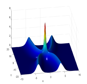
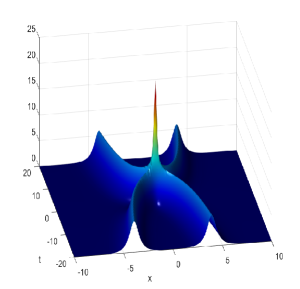
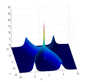
(a)               (b)           (c)

Figure 1. (Color online) The surface plots of $|u(x,t)|^{2}+|v(x,t)|^{2}$ for the exponential double-soliton solutions with (a) $\gamma=\frac{\pi}{3}$, (b) $\gamma=\frac{2\pi}{3}$, and (c) $\gamma=\frac{5\pi}{6}$.

We shall find the approximate distance between the two identical solitons for large $|x|+|t|$. It follows from the bilinear equations, see [4, 8] and Appendix B, that

$$|u|^{2}+|v|^{2}=\frac{|N_{u}|^{2}+|N_{v}|^{2}}{|D(M)|^{2}}=2i\frac{\partial}{\partial x}\log\frac{\overline{D(M)}}{D(M)}.$$ (3.35)

Therefore, we just need to investigate the behavior of $D(M)$ for large $|x|+|t|$. The dominant terms of $D(M)$ as $|x|+|t|\to\infty$ are given by

$$D(M)\sim e^{-2x\sin\gamma-i\gamma}\left(e^{-2x\sin\gamma-i\gamma}+4(\sin\gamma)^{4}t^{2}\right),$$

from which we obtain that

$$|x|\sim\frac{\ln|t|}{\sin\gamma},\quad\mbox{\rm as}\;\;|x|+|t|\to\infty.$$ (3.36)

The dependence (3.36) is shown in Figure 2 by red line together with the contour plots from Figure 1.

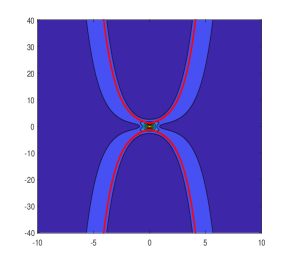
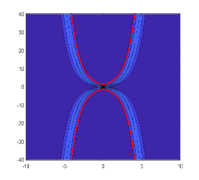
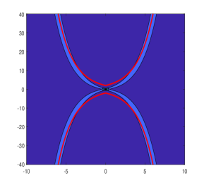
(a)               (b)           (c)

Figure 2. (Color online) The contour plots of $|u(x,t)|^{2}+|v(x,t)|^{2}$ for the solutions of Figure 1 with (a) $\gamma=\frac{\pi}{3}$, (b) $\gamma=\frac{2\pi}{3}$, (c) $\gamma=\frac{5\pi}{6}$.

4. Limit to the algebraic double-solitons

Here we take the limit $\gamma\to\pi$ of the exponential double-solitons in Theorem 2.1 to derive the algebraic double-solitons. We show that the algebraic double-solitons correspond to the double embedded eigenvalue $\zeta_{0}=i$ in the linear systems (2.30) and (2.31). In order to obtain nontrivial limits, we change the arbitrary parameters $\tilde{x}_{0}$ and $\tilde{t}_{0}$ used in Section 3 with the transformation

$$\tilde{x}_{0}\to\tilde{x}_{0}+\frac{1}{\sin\gamma},\qquad\tilde{t}_{0}\to\tilde{t}_{0}+\frac{1}{2\sin\gamma}.$$ (4.1)

The two computations below give the proof of Theorem 2.3.

4.1. Computations of (2.32) and (2.33)

Let $\gamma:=\pi-\varepsilon$ and consider the limit $\varepsilon\to 0^{+}$. Taylor’s expansions yield

$$\sin\gamma =\varepsilon-\frac{1}{6}\varepsilon^{3}+\mathcal{O}(\varepsilon^{5}),$$

$$\cos\gamma =-1+\frac{\varepsilon^{2}}{2}+\mathcal{O}(\varepsilon^{4}).$$

To obtain (2.32) and (2.33), we only need to substitute (4.1) into $D(M)$, $N_{u}$ and $N_{v}$ given below (2.29) and collect together the coefficients of Taylor expanion at powers $\varepsilon$, $\varepsilon^{2}$, $\varepsilon^{3}$, and $\varepsilon^{4}$. With the transformation (4.1), we rewrite $D(M)$ as

$$D(M) =1+e^{-4x\sin\gamma-2i\gamma}+2e^{-2x\sin\gamma-i\gamma}$$

$$\quad\times\left(1+2(\sin\gamma)^{2}\left[(x-\tilde{x}_{0})\cos\gamma+\frac{i}{2}\right]^{2}+2(\sin\gamma)^{4}(t-\tilde{t}_{0})^{2}\right).$$

Expansion as $\varepsilon\to 0$ gives nonzero terms at powers $\varepsilon^{2}$, $\varepsilon^{3}$, and $\varepsilon^{4}$:

$$\varepsilon^{2}:\qquad -4\tilde{x}_{0}(i-2x+\tilde{x}_{0}),$$

$$\varepsilon^{3}:\qquad -4\tilde{x}_{0}(i-2x)(i-2x+\tilde{x}_{0}),$$

$$\varepsilon^{4}:\qquad \frac{1}{12}(i-2x)^{4}+\frac{1}{3}(i-2x)(i-6x)-4(t-\tilde{t}_{0})^{2}-2\tilde{x}_{0}(i-2x)^{2}(i-2x+\tilde{x}_{0})$$

$$\quad+\frac{2}{3}\tilde{x}_{0}(8\tilde{x}_{0}-16x+5i).$$

With the transformation (4.1), we rewrite $N_{u}$ and $N_{v}$ as

$$N_{u} =4i(\sin\gamma)^{2}e^{-x\sin\gamma+it\cos\gamma-\frac{i\gamma}{2}}\left(-\cot\gamma+(x-\tilde{x}_{0})\cos\gamma+i(t-\tilde{t}_{0})\sin\gamma+\frac{i}{2}\right.$$

$$\left.\quad-e^{-2x\sin\gamma-i\gamma}\left[\cot\gamma+(x-\tilde{x}_{0})\cos\gamma-i(t-\tilde{t}_{0})\sin\gamma+\frac{i}{2}\right]\right)$$

and

$$N_{v} =4i(\sin\gamma)^{2}e^{-x\sin\gamma-it\cos\gamma-\frac{i\gamma}{2}}\left(-\cot\gamma+(x-\tilde{x}_{0})\cos\gamma-i(t-\tilde{t}_{0})\sin\gamma+\frac{i}{2}\right.$$

$$\left.\quad-e^{-2x\sin\gamma-i\gamma}\left[\cot\gamma+(x-\tilde{x}_{0})\cos\gamma+i(t-\tilde{t}_{0})\sin\gamma+\frac{i}{2}\right]\right).$$

The expression in the circular brackets for $N_{u}$ and $N_{v}$ are multiplied by

$$4i(\sin\gamma)^{2}e^{-x\sin\gamma\pm it\cos\gamma-\frac{i\gamma}{2}}\sim 4\varepsilon^{2}e^{\mp it}\quad\mbox{\rm as}\quad\varepsilon\to 0.$$

Since the expansions of the exponential factors in powers of $\varepsilon$ do not modify the limit of $\varepsilon\to 0$, we collect nonzero terms in the expansions of $N_{u}e^{-it\cos\gamma}$ and $N_{v}e^{it\cos\gamma}$ at powers $\varepsilon^{2}$, $\varepsilon^{3}$, and $\varepsilon^{4}$:

$$\varepsilon^{2}:\qquad 8\tilde{x}_{0},$$

$$\varepsilon^{3}:\qquad 4\tilde{x}_{0}(i-2x),$$

$$\varepsilon^{4}:\qquad \frac{1}{3}(i-2x)^{3}+5\tilde{x}_{0}(i-2x)^{2}-4i(t-\tilde{t}_{0})(i-2x)+\frac{4i}{3}-\frac{20}{3}\tilde{x}_{0},$$

and

$$\varepsilon^{2}:\quad 8\tilde{x}_{0},$$

$$\varepsilon^{3}:\quad 4\tilde{x}_{0}(i-2x),$$

$$\varepsilon^{4}:\quad \frac{1}{3}(i-2x)^{3}+5\tilde{x}_{0}(i-2x)^{2}+4i(t-\tilde{t}_{0})(i-2x)+\frac{4i}{3}-\frac{20}{3}\tilde{x}_{0}.$$

By rescaling $\tilde{x}_{0}\to\tilde{x}_{0}\varepsilon^{2}$, we now obtain the nontrivial limit at the power $\varepsilon^{4}$:

$$\lim_{\varepsilon\to 0}D(M)\varepsilon^{-4} =\frac{4}{3}x^{4}-\frac{8}{3}ix^{3}+2x^{2}-2ix-\frac{1}{4}-4(t-\tilde{t}_{0})^{2}-4\tilde{x}_{0}(i-2x),$$

$$\lim_{\varepsilon\to 0}N_{u}e^{it}\varepsilon^{-4} =-\frac{8}{3}x^{3}+4ix^{2}+2x+i-4i(t-\tilde{t}_{0})(i-2x)+8\tilde{x}_{0},$$

$$\lim_{\varepsilon\to 0}N_{v}e^{-it}\varepsilon^{-4} =-\frac{8}{3}x^{3}+4ix^{2}+2x+i+4i(t-\tilde{t}_{0})(i-2x)+8\tilde{x}_{0},$$

which yields the explicit expressions (2.32) and (2.33) from the quotients given by (2.29).

4.2. Computations of (2.34) and (2.35)

We substitute the phase shift (4.1) into $n_{1}^{(+)}(\lambda_{0})$ and $(n_{1}^{(+)})^{\prime}(\lambda_{0})$ given in (3.30) and (3.34). These expressions define the eigenvector and the generalized eigenvector of the linear systems (2.30) and (2.31) for $\zeta_{0}=e^{\frac{i\gamma}{2}}$ by (3.27) and (3.31) respectively. By using $\gamma:=\pi-\varepsilon$ and expanding in powers of $\varepsilon$, we derive (2.34) and (2.35).

After the transformation (4.1), we rewrite $M_{22}$ and $-\bar{C}_{0}\bar{\lambda}_{0}e^{-2i\theta(\bar{\lambda}_{0})}(M_{22}b_{1}+M_{12}b_{2})$ in (3.30) as follows:

$$M_{22}=1+(\sin\gamma)e^{-2x\sin\gamma}\left(\cot\gamma+2(x-\tilde{x}_{0})\cos\gamma-2i(t-\tilde{t}_{0})\sin\gamma\right)$$

and

$$-\bar{C}_{0}\bar{\lambda}_{0}e^{-2i\theta(\bar{\lambda}_{0})}(M_{22}b_{1}+M_{12}b_{2})=-e^{-x\sin\gamma-it\cos\gamma-\frac{3i\gamma}{2}}$$

$$\qquad\qquad\times\left(e^{i\gamma}+2\sin\gamma\left[-\cot\gamma+(x-\tilde{x}_{0})\cos\gamma-i(t-\tilde{t}_{0})\sin\gamma+\frac{i}{2}\right]-e^{-2x\sin\gamma-2i\gamma}\right).$$

Expansion as $\varepsilon\to 0$ gives nonzero terms at powers $\varepsilon^{1}$, and $\varepsilon^{2}$.

• The coefficients of $M_{22}$:

  $$\varepsilon^{1}:\quad 2\tilde{x}_{0},$$

  $$\varepsilon^{2}:\quad 2x^{2}-2i(t-\tilde{t}_{0})+\frac{1}{2}-4x\tilde{x}_{0}.$$

• The coefficients of $-\bar{C}_{0}\bar{\lambda}_{0}e^{-2i\theta(\bar{\lambda}_{0})}(M_{22}b_{1}+M_{12}b_{2})e^{it\cos\gamma}$:

  $$\varepsilon^{1}:\quad -2i\tilde{x}_{0},$$

  $$\varepsilon^{2}:\quad 2ix^{2}+4x-2(t-\tilde{t}_{0})-\frac{3}{2}i+3\tilde{x}_{0}+2ix\tilde{x}_{0}.$$

Rescaling $\tilde{x}_{0}\to\tilde{x}_{0}\varepsilon^{2}$ yields the nontrivial limit at the power $\varepsilon^{2}$:

$$\lim_{\varepsilon\to 0} M_{22}\varepsilon^{-2}=2x^{2}-2i(t-\tilde{t}_{0})+\frac{1}{2},$$

$$\lim_{\varepsilon\to 0} \left(-\bar{C}_{0}\bar{\lambda}_{0}e^{-2i\theta(\bar{\lambda}_{0})}(M_{22}b_{1}+M_{12}b_{2})e^{-it}\right)\varepsilon^{-2}=-2ix^{2}-4x+2(t-\tilde{t}_{0})+\frac{3}{2}i.$$

By using (3.27) and (3.30), taking the limit

$$\psi_{0}:=\lim_{\varepsilon\to 0}\varepsilon^{2}\psi^{(+)}_{1}(\zeta_{0}),$$

we obtain (2.34) with

$$\mathfrak{n}_{0}:=\lim_{\varepsilon\to 0}\varepsilon^{2}n^{(+)}_{1}(\lambda_{0})$$

given below (2.34) in the explicit form.

To obtain a nontrivial limit for the generalized eigenvector, we rewrite the expression (3.31) in the equivalent form:

$$(\psi^{(+)}_{1})^{\prime}(\zeta_{0})-2(\lambda_{0}-\bar{\lambda}_{0})^{-1}\psi^{(+)}_{1}(\zeta_{0})$$

$$=2\zeta_{0}e^{i\theta(\lambda_{0})}[T(v,\zeta_{0})]^{-1}\left[(n_{1}^{(+)})^{\prime}(\lambda_{0})+\left(i\theta^{\prime}(\lambda_{0})-2(\lambda_{0}-\bar{\lambda}_{0})^{-1}\right)n_{1}^{(+)}(\lambda_{0})\right]$$

$$\qquad-\zeta_{0}^{-1}\partial_{\zeta}T(v,\zeta)\psi^{(+)}_{1}(\zeta_{0}),$$

After the transformation (4.1), we rewrite $-M_{21}$ and $\bar{C}_{0}\bar{\lambda}_{0}e^{-2i\theta(\bar{\lambda}_{0})}(M_{11}b_{2}+M_{21}b_{1})$ in (3.34) as follows:

$$-M_{21}=-2ie^{-2x\sin\gamma-i\gamma}\left[\sin\gamma\left[(x-\tilde{x}_{0})^{2}(\cos\gamma)^{2}+(t-\tilde{t}_{0})^{2}(\sin\gamma)^{2}\right]+i(t-\tilde{t}_{0})\sin\gamma\cos\gamma+\frac{\sin\gamma}{4}\right]$$

and

$$\bar{C}_{0}\bar{\lambda}_{0}e^{-2i\theta(\bar{\lambda}_{0})}(M_{11}b_{2}+M_{21}b_{1})=-ie^{-x\sin\gamma-it\cos\gamma-\frac{3i}{2}\gamma}$$

$$\qquad\times\left((x-\tilde{x}_{0})\cos\gamma-i(t-\tilde{t}_{0})\sin\gamma+\frac{i}{2}+e^{-2x\sin\gamma-3i\gamma}\left[(x-\tilde{x}_{0})\cos\gamma+i(t-\tilde{t}_{0})\sin\gamma+\frac{i}{2}\right]\right).$$

Expansion as $\varepsilon\to 0$ gives nonzero terms at powers $\varepsilon^{0}$, $\varepsilon^{1}$, and $\varepsilon^{2}$ for both components of the numerator of $(n_{1}^{(+)})^{\prime}(\lambda_{0})+\left(i\theta^{\prime}(\lambda_{0})-2(\lambda_{0}-\bar{\lambda}_{0})^{-1}\right)n_{1}^{(+)}(\lambda_{0})$.

• The coefficients of $-M_{21}+\left(i\theta^{\prime}(\lambda_{0})-2(\lambda_{0}-\bar{\lambda}_{0})^{-1}\right)M_{22}$:

  $$\varepsilon^{0}:\quad -2i\tilde{x}_{0},$$

  $$\varepsilon^{1}:\quad ix\tilde{x}_{0}+2i\tilde{x}_{0}^{2},$$

  $$\varepsilon^{2}:\quad \frac{4}{3}i\tilde{x}_{0}+x(t-\tilde{t}_{0})-\frac{1}{3}ix^{3}+2ix^{2}\tilde{x}_{0}-\frac{4}{3}ix+\tilde{x}_{0}t$$

  $$+3x\tilde{x}_{0}-4ix\tilde{x}_{0}^{2}-2x^{2}-2\tilde{x}_{0}^{2}-\frac{1}{2}+2i(t-\tilde{t}_{0}).$$

• The coefficients of

  $$\bar{C}_{0}\bar{\lambda}_{0}e^{-2i\theta(\bar{\lambda}_{0})}\left[M_{11}b_{2}+M_{21}b_{1}-\left(i\theta^{\prime}(\lambda_{0})-2(\lambda_{0}-\bar{\lambda}_{0})^{-1}\right)(M_{22}b_{1}+M_{12}b_{2})\right]e^{it\cos\gamma}:$$

  $$e^{it}\varepsilon^{2}:\quad -2\tilde{x}_{0},$$

  $$e^{it}\varepsilon^{3}:\quad 6i\tilde{x}_{0}-5x\tilde{x}_{0},$$

  $$e^{it}\varepsilon^{4}:\quad ix(t-\tilde{t}_{0})-it\tilde{x}_{0}-ix^{2}+\frac{5}{4}i-\frac{1}{3}x^{3}-\frac{15}{4}x$$

  $$+3(t-\tilde{t}_{0})+\frac{155}{12}\tilde{x}_{0}-6x^{2}\tilde{x}_{0}-it\tilde{x}_{0}+\frac{35}{2}ix\tilde{x}_{0}.$$

Rescaling $\tilde{x}_{0}\to\tilde{x}_{0}\varepsilon^{2}$ yields the nontrivial limit at the power $\varepsilon^{2}$:

$$\lim_{\varepsilon\to 0}\left[-M_{21}+\left(i\theta^{\prime}(\lambda_{0})-2(\lambda_{0}-\bar{\lambda}_{0})^{-1}\right)M_{22}\right]\varepsilon^{-2}$$

$$=-\frac{1}{3}ix^{3}-2x^{2}-\frac{4}{3}ix+x(t-\tilde{t}_{0})+2i(t-\tilde{t}_{0})-\frac{1}{2}-2i\tilde{x}_{0},$$

$$\lim_{\varepsilon\to 0}\bar{C}_{0}\bar{\lambda}_{0}e^{-2i\theta(\bar{\lambda}_{0})}\left[M_{11}b_{2}+M_{21}b_{1}-\left(i\theta^{\prime}(\lambda_{0})-2(\lambda_{0}-\bar{\lambda}_{0})^{-1}\right)(M_{22}b_{1}+M_{12}b_{2})\right]e^{-it}\varepsilon^{-2}$$

$$=-\frac{1}{3}x^{3}-ix^{2}-\frac{15}{4}x+ix(t-\tilde{t}_{0})+\frac{5}{4}i+3(t-\tilde{t}_{0})-2\tilde{x}_{0}.$$

By using (3.31) and (3.34), taking the limit

$$\psi_{1}:=\lim_{\varepsilon\to 0}\varepsilon^{2}\left[(\psi^{(+)}_{1})^{\prime}(\zeta_{0})-2(\lambda_{0}-\bar{\lambda}_{0})^{-1}\psi^{(+)}_{1}(\zeta_{0})\right],$$

we obtain (2.35) with

$$\mathfrak{n}_{1}:=\lim_{\varepsilon\to 0}\varepsilon^{2}\left[(n_{1}^{(+)})^{\prime}(\lambda_{0})+\left(i\theta^{\prime}(\lambda_{0})-2(\lambda_{0}-\bar{\lambda}_{0})^{-1}\right)n_{1}^{(+)}(\lambda_{0})\right]$$

given below (2.35) in the explicit form.

Appendix A Single-soliton from a simple pole

Here we consider solutions of the normalized RH problem for the refelectionless potential $r_{\pm}(\lambda)\equiv 0$ for $\lambda\in\mathbb{R}$ with a simple pole at $\lambda_{0}\in\mathbb{C}^{+}$. By symmetry (2.9), both $\lambda_{0}\in\mathbb{C}^{+}$ and $\bar{\lambda}_{0}\in\mathbb{C}^{-}$ are poles of $M(\lambda)$ in $\mathbb{C}$. The normalized RH problem can be rewritten in the form:

RH problem. Find a complex-valued function $M(\lambda)$ with the following properties: • $M(\lambda)$ has simple poles at $\lambda_{0}\in\mathbb{C}^{+}$ and $\bar{\lambda}_{0}\in\mathbb{C}^{-}$. • $M(\lambda)\to\mathbb{I}$ as $|\lambda|\to\infty$, where $\mathbb{I}$ is the $2$-by-$2$ identity matrix. • $M_{+}(\lambda)=M_{-}(\lambda)$ for every $\lambda\in\mathbb{R}$, where $M_{\pm}(\lambda):=\lim\limits_{{\rm Im}(\lambda)\to\pm 0}M(\lambda)$.

The solution of the RH problem is immediately given by

$$M(x,t,\lambda)=\mathbb{I}+\frac{{\rm Res}_{\lambda=\lambda_{0}}M_{+}(\lambda)}{\lambda-\lambda_{0}}+\frac{{\rm Res}_{\lambda=\bar{\lambda}_{0}}M_{-}(\lambda)}{\lambda-\bar{\lambda}_{0}}.$$ (A.1)

In order to compute the residue terms, we note from (2.21) that $\lambda_{0}$ is a simple zero of $\alpha(\lambda)$ extended to $\mathbb{C}^{+}$ by Lemma 2.2. Since it follows from (2.4) that

$$\alpha(\lambda)=a(\zeta)=\det\left(\psi^{(+)}_{1}(\zeta),\psi^{(-)}_{2}(\zeta)\right),$$

we define $\zeta_{0}:=\sqrt{\lambda_{0}}$ and a constant $b_{0}\in\mathbb{C}$ such that the columns of $\psi^{(\pm)}(\zeta)$ satisfying (2.1) are related at $\zeta=\zeta_{0}$ by

$$\psi^{(-)}_{2}(\zeta_{0})=b_{0}\psi^{(+)}_{1}(\zeta_{0}).$$ (A.2)

Since $\lambda_{0}\in\mathbb{C}^{+}$, it follows from (2.1) and (A.2) that $\psi^{(-)}_{2}(\zeta_{0})$ decays to zero exponentially fast both as $x\to\pm\infty$. Hence it is the eigenvector of the linear system (1.2) for $\zeta=\zeta_{0}$.

By using the transformation (2.12), we can rewrite (A.2) in the form:

$$n^{(-)}_{2}(\lambda_{0})=b_{0}\zeta_{0}^{-1}n^{(+)}_{1}(\lambda_{0})e^{2i\theta(\lambda_{0})},$$ (A.3)

where $\theta(\lambda)$ is given by (2.18). By using (2.21) and (A.3), we compute the residue term as follows

$${\rm Res}_{\lambda=\lambda_{0}}P(\lambda)=\left(\vec{\bf 0}\quad\frac{n^{(-)}_{2}(\lambda_{0})}{\alpha^{\prime}(\lambda_{0})}\right)=\left(\vec{\textbf{0}}\quad\frac{b_{0}}{\zeta_{0}\alpha^{\prime}(\lambda_{0})}n^{(+)}_{1}(\lambda_{0})e^{2i\theta(\lambda_{0})}\right),$$ (A.4)

where $\vec{\textbf{0}}$ is the $2$-by-$1$ null vector.

By using the symmetry condition (2.9), we have

$$\psi_{1}^{(\pm)}(\zeta)=\left(\begin{array}[]{cc}0&1\\ -1&0\\ \end{array}\right)\overline{\psi}_{2}^{(\pm)}(\zeta),\quad\psi_{2}^{(\pm)}(\zeta)=\left(\begin{array}[]{cc}0&-1\\ 1&0\\ \end{array}\right)\overline{\psi}_{1}^{(\pm)}(\zeta),$$

then (A.2) can be transformed into

$$\psi^{(-)}_{1}(\bar{\zeta}_{0})=-\bar{b}_{0}\psi^{(+)}_{2}(\bar{\zeta}_{0}).$$

Using the transformation (2.12), we obtain

$$n^{(-)}_{1}(\bar{\lambda}_{0})=-\bar{b}_{0}\bar{\zeta}_{0}n^{(+)}_{2}(\bar{\lambda}_{0})e^{-2i\theta(\bar{\lambda}_{0})},$$ (A.5)

from which we compute the other residue term by using (2.21) and (A.5):

$${\rm Res}_{\lambda=\bar{\lambda}_{0}}P(\lambda)=\left(\frac{n^{(-)}_{1}(\bar{\lambda}_{0})}{\bar{\alpha}^{\prime}(\bar{\lambda}_{0})}\quad\vec{\bf 0}\right)=\left(-\frac{\bar{b}_{0}\bar{\zeta}_{0}}{\bar{\alpha}^{\prime}(\bar{\lambda}_{0})}n^{(+)}_{2}(\bar{\lambda}_{0})e^{-2i\theta(\bar{\lambda}_{0})}\quad\vec{\textbf{0}}\right),$$ (A.6)

We recall that $M(\lambda)=[P^{\infty}]^{-1}P(\lambda)$ with $P^{\infty}={\rm diag}(n_{1}^{+\infty},n_{2}^{+\infty})$ with $n_{2}^{+\infty}=\overline{n_{1}^{+\infty}}$, see (2.24). Using the first column of (A.1) at $\lambda=\lambda_{0}$ due to (A.4) and the second column of (A.1) at $\lambda=\bar{\lambda}_{0}$ due to (A.6), we obtain a closed system of linear algebraic equations:

$$n^{(+)}_{1}(\lambda_{0})=n_{1}^{+\infty}e_{1}-\frac{\bar{\lambda}_{0}\bar{c}_{0}}{\lambda_{0}-\bar{\lambda}_{0}}n^{(+)}_{2}(\bar{\lambda}_{0})e^{-2i\theta(\bar{\lambda}_{0})}$$ (A.7)

and

$$n^{(+)}_{2}(\bar{\lambda}_{0})=n_{2}^{+\infty}e_{2}+\frac{c_{0}}{\bar{\lambda}_{0}-\lambda_{0}}n^{(+)}_{1}(\lambda_{0})e^{2i\theta(\lambda_{0})},$$ (A.8)

where $e_{1}=(1,0)^{T}$, $e_{2}=(0,1)^{T}$, and

$$c_{0}:=\frac{b_{0}}{\zeta_{0}\alpha^{\prime}(\zeta_{0})}.$$

Then, from (A.7) and (A.8), we have

$$n^{(+)}_{1}(\lambda_{0}) =n^{+\infty}_{1}e_{1}-\frac{\bar{\lambda}_{0}\bar{c}_{0}}{\lambda_{0}-\bar{\lambda}_{0}}n_{2}^{+\infty}e^{-2i\theta(\bar{\lambda}_{0})}e_{2}+\frac{\bar{\lambda}_{0}|c_{0}|^{2}}{(\lambda_{0}-\bar{\lambda}_{0})^{2}}e^{2i\theta(\lambda_{0})-2i\theta(\bar{\lambda}_{0})}n^{(+)}_{1}(\lambda_{0}),$$

$$n^{(+)}_{2}(\bar{\lambda}_{0}) =n^{+\infty}_{2}e_{2}+\frac{c_{0}}{\bar{\lambda}_{0}-\lambda_{0}}n^{+\infty}_{1}e^{2i\theta(\lambda_{0})}e_{1}+\frac{\bar{\lambda}_{0}|c_{0}|^{2}}{(\lambda_{0}-\bar{\lambda}_{0})^{2}}e^{2i\theta(\lambda_{0})-2i\theta(\bar{\lambda}_{0})}n^{(+)}_{2}(\bar{\lambda}_{0}).$$

By using (2.25), we obtain the explicit solutions to the MTM system (1.1) in the form

$$u=\lim_{\lambda\to 0}\overline{M}_{12}(\lambda)=-\frac{\bar{c}_{0}}{\bar{\lambda}_{0}}n_{1}^{+\infty}\overline{n^{(+)}_{11}(\lambda_{0})}e^{-2i\theta(\bar{\lambda}_{0})}=-\frac{\bar{c}_{0}e^{-2i\theta(\bar{\lambda}_{0})}}{\bar{\lambda}_{0}-\frac{|\lambda_{0}|^{2}|c_{0}|^{2}}{(\lambda_{0}-\bar{\lambda}_{0})^{2}}e^{2i\theta(\lambda_{0})-2i\theta(\bar{\lambda}_{0})}}$$

and

$$v=\lim_{\lambda\to 0}M_{21}(\lambda)=\bar{c}_{0}n_{1}^{+\infty}(x)n^{(+)}_{22}(\bar{\lambda}_{0})e^{-2i\theta(\bar{\lambda}_{0})}=\frac{\bar{c}_{0}e^{-2i\theta(\bar{\lambda}_{0})}}{1-\frac{\bar{\lambda}_{0}|c_{0}|^{2}}{(\lambda_{0}-\bar{\lambda}_{0})^{2}}e^{2i\theta(\lambda_{0})-2i\theta(\bar{\lambda}_{0})}}.$$

To simplify the expressions for the single-soliton solution $(u,v)$, we pick $\lambda_{0}=e^{i\gamma}$ with $\gamma\in(0,\pi)$ on $\mathbb{S}^{1}\cap\mathbb{C}^{+}$. A more general solution can be obtained with the Lorentz symmetry (2.26). If $\lambda_{0}=e^{i\gamma}$, we obtain from (2.18) that

$$2i\theta(\lambda_{0})=-\alpha x+i\beta t,$$

where $\alpha=\sin\gamma$ and $\beta=\cos\gamma$. In addition, we choose

$$c_{0}=2i\sin\gamma e^{\frac{i\gamma}{2}}$$

and obtain the single-soliton solution in the form

$$u(x,t)=2i\alpha\frac{e^{-\alpha x-i\beta t+\frac{i\gamma}{2}}}{1+e^{-2\alpha x+i\gamma}}=i\alpha\;{\rm sech}\left(\alpha x-\frac{i\gamma}{2}\right)\;e^{-i\beta t}$$ (A.9)

and

$$v(x,t)=-2i\alpha\;\frac{e^{-\alpha x-i\beta t-\frac{i\gamma}{2}}}{1+e^{-2\alpha x-i\gamma}}=-i\alpha\;{\rm sech}\left(\alpha x+\frac{i\gamma}{2}\right)\;e^{-i\beta t},$$ (A.10)

which coincides with (2.28) since $\alpha=\sin\gamma$ and $\beta=\cos\gamma$. A more general solution with two translational parameters $x_{0},t_{0}\in\mathbb{R}$ can be obtained by using the symmetries (2.27) or by introducing two translational parameters in the expression for $c_{0}\in\mathbb{C}$.

Finally, we write the explicit form of the eigenvector $\psi_{1}^{(+)}(\zeta_{0})$, see (A.2), which satisfies (2.30) with $(u,v)$ given by (A.9)–(A.10) and with $\zeta_{0}=e^{\frac{i\gamma}{2}}$. By using the transformation (2.12), we write

$$\psi^{(+)}_{1}(\zeta_{0})=e^{i\theta(\lambda_{0})}[T(v,\zeta_{0})]^{-1}n_{1}^{(+)}(\lambda_{0}),$$

where

$$[T(v,\zeta_{0})]^{-1}=\left(\begin{matrix}1&0\\ -e^{-\frac{i\gamma}{2}}v&e^{-\frac{i\gamma}{2}}\end{matrix}\right)$$

and

$$n_{1}^{(+)}(\lambda_{0}) =\frac{n^{+\infty}_{1}e_{1}-\frac{\bar{\lambda}_{0}\bar{c}_{0}}{\lambda_{0}-\bar{\lambda}_{0}}n_{2}^{+\infty}e^{-2i\theta(\bar{\lambda}_{0})}e_{2}}{1-\frac{\bar{\lambda}_{0}|c_{0}|^{2}}{(\lambda_{0}-\bar{\lambda}_{0})^{2}}e^{2i\theta(\lambda_{0})-2i\theta(\bar{\lambda}_{0})}}$$

$$=\frac{1}{1+e^{-2\alpha x-i\gamma}}\left(\begin{array}[]{c}n_{1}^{+\infty}\\ e^{-\alpha x-i\beta t-\frac{3i\gamma}{2}}n_{2}^{+\infty}\end{array}\right)$$

$$=\frac{1}{2}{\rm sech}\left(\alpha x+\frac{i\gamma}{2}\right)\left(\begin{array}[]{c}e^{\alpha x+\frac{i\gamma}{2}+\frac{i}{4}\int_{+\infty}^{x}(|u|^{2}+|v|^{2})dx}\\ e^{-i\beta t-i\gamma-\frac{i}{4}\int_{+\infty}^{x}(|u|^{2}+|v|^{2})dx}\end{array}\right).$$

We note that

$$\frac{1}{4}\int_{\mathbb{R}}(|u|^{2}+|v|^{2})dx=\int_{\mathbb{R}}\frac{\sin^{2}\gamma}{\cosh(2\sin\gamma\;x)+\cos\gamma}dx=\gamma.$$

Hence we can write

$$e^{i\theta(\lambda_{0})}n_{1}^{(+)}(\lambda_{0})=\frac{1}{2}{\rm sech}\left(\alpha x+\frac{i\gamma}{2}\right)\left(\begin{array}[]{c}e^{\frac{1}{2}\alpha x+\frac{i}{2}\beta t+\frac{i\gamma}{2}+\frac{i}{4}\int_{+\infty}^{x}(|u|^{2}+|v|^{2})dx}\\ e^{-\frac{1}{2}\alpha x-\frac{i}{2}\beta t-\frac{i}{4}\int_{-\infty}^{x}(|u|^{2}+|v|^{2})dx}\end{array}\right),$$ (A.11)

which decays exponentially to $0$ as $x\to\pm\infty$. Since $[T(v,\zeta_{0})]^{-1}$ is bounded, then $\psi^{(+)}_{1}(\zeta_{0})\in H^{1}(\mathbb{R},\mathbb{C}^{2})$ is an exponentially decaying eigenvector of the linear system (2.30).

The algebraic soliton appears in the singular limit $\gamma\to\pi$, where $\zeta_{0}\to i$. The simple eigenvalue $\zeta_{0}=i$ is embedded into the continuous spectrum of the Lax system (1.2), which is located on $\mathbb{R}\cup(i\mathbb{R})$. By writing $\gamma:=\pi-\epsilon$ and taking the limit $\epsilon\to 0$ in (A.9) and (A.10), we obtain

$$u(x,t)=\frac{2i}{1-2ix}e^{it},\quad v(x,t)=-\frac{2i}{1+2ix}e^{it}.$$ (A.12)

The eigenvector $\psi_{0}$ for the simple embedded eigenvalue $\zeta_{0}=i$ of the linear system (2.30) with $(u,v)$ given by (A.12) is obtained from (A.11) in the limit $\epsilon\to 0$ in the explicit form:

$$\psi_{0}:=\lim_{\epsilon\to 0}\epsilon\psi^{(+)}_{1}(\zeta_{0})=\frac{1}{1+2ix}\left(\begin{matrix}1&0\\ iv&-i\end{matrix}\right)\left(\begin{array}[]{c}e^{-\frac{it}{2}+i\arctan(2x)}\\ e^{\frac{it}{2}-\frac{i\pi}{2}-i\arctan(2x)}\end{array}\right),$$ (A.15)

where we have used the elementary integral

$$\frac{1}{4}\int_{-\infty}^{x}(|u|^{2}+|v|^{2})dx=\int_{-\infty}^{x}\frac{2}{1+4x^{2}}dx=\frac{\pi}{2}+\arctan(2x).$$

Based on the explicit expression (A.15), we confirm that $\psi_{0}\in H^{1}(\mathbb{R},\mathbb{C}^{2})$ is an algebraically decaying eigenvector of the linear system (2.30) such that $|\psi_{0}(x)|=\mathcal{O}(|x|^{-1})$ as $|x|\to\infty$.

Appendix B Exponential double-solitons in the bilinear Hirota method

Here we obtain the exponential double-soliton solutions by using the bilinear Hirota method developed in [4]. To proceed with computations, we use the parameterization from [8] and write the general exponential two-soliton solutions in the form:

$$u=\frac{g}{\bar{f}},\quad v=\frac{h}{f},$$ (B.1)

where

$$f =1+e^{-2\xi_{1}-\mathrm{i}\gamma_{1}}+e^{-2\xi_{2}-\mathrm{i}\gamma_{2}}+A_{12}e^{-2\xi_{1}-2\xi_{2}-\mathrm{i}\gamma_{1}-\mathrm{i}\gamma_{2}}-4\sqrt{\delta_{1}\delta_{2}}\sin\gamma_{1}\sin\gamma_{2}e^{-\xi_{1}-\xi_{2}-\frac{\mathrm{i}}{2}\gamma_{1}-\frac{\mathrm{i}}{2}\gamma_{2}}$$

$$\quad\times\left[\frac{\delta_{1}e^{-\mathrm{i}(\eta_{1}-\eta_{2})}}{(\delta_{1}e^{-\frac{\mathrm{i}}{2}(\gamma_{1}+\gamma_{2})}-\delta_{2}e^{\frac{\mathrm{i}}{2}(\gamma_{1}+\gamma_{2})})^{2}}+\frac{\delta_{2}e^{\mathrm{i}(\eta_{1}-\eta_{2})}}{(\delta_{1}e^{\frac{\mathrm{i}}{2}(\gamma_{1}+\gamma_{2})}-\delta_{2}e^{-\frac{\mathrm{i}}{2}(\gamma_{1}+\gamma_{2})})^{2}}\right],$$

$$h =-\bar{\alpha}_{1}e^{-\xi_{1}-\mathrm{i}\eta_{1}}\left[1+\left(\frac{p_{1}-p_{2}}{p_{1}+\bar{p}_{2}}\right)^{2}e^{-2\xi_{2}+\mathrm{i}\gamma_{2}}\right]-\bar{\alpha}_{2}e^{-\xi_{2}-\mathrm{i}\eta_{2}}\left[1+\left(\frac{p_{1}-p_{2}}{\bar{p}_{1}+p_{2}}\right)^{2}e^{-2\xi_{1}+\mathrm{i}\gamma_{1}}\right],$$

and

$$g =\frac{\mathrm{i}\bar{\alpha}_{1}}{p_{1}}e^{-\xi_{1}-\mathrm{i}\eta_{1}}\left[1+\left(\frac{p_{1}-p_{2}}{p_{1}+\bar{p}_{2}}\right)^{2}e^{-2\xi_{2}+3\mathrm{i}\gamma_{2}}\right]+\frac{\mathrm{i}\bar{\alpha}_{2}}{p_{2}}e^{-\xi_{2}-\mathrm{i}\eta_{2}}\left[1+\left(\frac{p_{1}-p_{2}}{\bar{p}_{1}+p_{2}}\right)^{2}e^{-2\xi_{1}+3\mathrm{i}\gamma_{1}}\right],$$

with arbitrary parameters $\gamma_{j}\in(0,\pi)$, $\delta_{j}>0$, $(x_{j},t_{j})\in\mathbb{R}^{2}$, and uniquely defined for $j=1,2$ as

$$p_{j}=\mathrm{i}\delta_{j}e^{-i\gamma_{j}},\quad\alpha_{j}=2\sqrt{\delta_{j}}\sin\gamma_{j}e^{\frac{\mathrm{i}\gamma_{j}}{2}},$$

$$\xi_{j} =\sin\gamma_{j}\left(\frac{1}{2}(\delta_{j}+\delta_{j}^{-1})x+\frac{1}{2}(\delta_{j}-\delta_{j}^{-1})t+x_{j}\right),$$

$$\eta_{j} =\cos\gamma_{j}\left(\frac{1}{2}(\delta_{j}-\delta_{j}^{-1})x+\frac{1}{2}(\delta_{j}+\delta_{j}^{-1})t+t_{j}\right),$$

and

$$A_{12}=\left(\frac{\delta_{1}^{2}+\delta_{2}^{2}-2\delta_{1}\delta_{2}\cos(\gamma_{1}-\gamma_{2})}{\delta_{1}^{2}+\delta_{2}^{2}-2\delta_{1}\delta_{2}\cos(\gamma_{1}+\gamma_{2})}\right)^{2}.$$

Due to Lorentz transformation (2.26), we can consider the exponential double-solitons with zero speed, for which we take $\delta_{1}=\delta_{2}=1$. In addition, we use translational symmetry and replace $e^{-\xi_{1,2}}$ by $e^{-\xi_{1,2}}\sin\left(\frac{\gamma_{1}+\gamma_{2}}{2}\right)$ in all expressions.

Considering $f$, we obtain

$$f =1+\sin^{2}\left(\frac{\gamma_{1}+\gamma_{2}}{2}\right)\left[e^{-2\xi_{1}-\mathrm{i}\gamma_{1}}+e^{-2\xi_{2}-\mathrm{i}\gamma_{2}}\right]+\sin^{4}\left(\frac{\gamma_{1}-\gamma_{2}}{2}\right)e^{-2\xi_{1}-2\xi_{2}-\mathrm{i}\gamma_{1}-\mathrm{i}\gamma_{2}}$$

$$\qquad+2\sin\gamma_{1}\sin\gamma_{2}e^{-\xi_{1}-\xi_{2}-\frac{\mathrm{i}}{2}\gamma_{1}-\frac{\mathrm{i}}{2}\gamma_{2}}\cos(\eta_{1}-\eta_{2}).$$

We now define the small parameter $\epsilon$ from $\gamma_{1}=\gamma+\epsilon$ and $\gamma_{2}=\gamma-\epsilon$ and take the limit $\epsilon\to 0$ for a given $\gamma\in(0,\pi)$. In order to get a nontrivial limit, we also define the translational parameters $x_{1,2}$ from the power series:

$$\xi_{1} =(\sin\gamma_{1})(x+x_{1})=\log(\epsilon)+\alpha(x-x_{0})+\epsilon\beta(x-\tilde{x}_{0})-\frac{1}{2}\epsilon^{2}\alpha(x-\tilde{\tilde{x}}_{0})+\mathcal{O}(\epsilon^{3}),$$

$$\xi_{2} =(\sin\gamma_{2})(x+x_{2})=\log(\epsilon)+\alpha(x-x_{0})-\epsilon\beta(x-\tilde{x}_{0})-\frac{1}{2}\epsilon^{2}\alpha(x-\tilde{\tilde{x}}_{0})+\mathcal{O}(\epsilon^{3}),$$

with new translational parameters $x_{0},\tilde{x}_{0},\tilde{\tilde{x}}_{0}\in\mathbb{R}$ and with $\alpha=\sin\gamma$, $\beta=\cos\gamma$. Similarly, we define the translational parameters $t_{1,2}$ from the power series:

$$\eta_{1} =(\cos\gamma_{1})(t+t_{1})=-\frac{\pi}{2}+\beta(t-t_{0})-\epsilon\alpha(t-\tilde{t}_{0})-\frac{1}{2}\epsilon^{2}\beta(t-\tilde{\tilde{t}}_{0})+\mathcal{O}(\epsilon^{3}),$$

$$\eta_{2} =(\cos\gamma_{2})(t+t_{2})=\frac{\pi}{2}+\beta(t-t_{0})+\epsilon\alpha(t-\tilde{t}_{0})-\frac{1}{2}\epsilon^{2}\beta(t-\tilde{\tilde{t}}_{0})+\mathcal{O}(\epsilon^{3}),$$

with new translational parameters $t_{0},\tilde{t}_{0},\tilde{\tilde{t}}_{0}\in\mathbb{R}$. With these choices, we expand the expression for $f$ in powers of $\epsilon$ and obtain the following explicit expression

$$\lim_{\epsilon\to 0}f=1+e^{-2\xi-i\gamma}\left[2+\alpha^{2}(2\beta(x-\tilde{x}_{0})+i)^{2}+4\alpha^{4}(t-\tilde{t}_{0})^{2}\right]+e^{-4\xi-2i\gamma},$$ (B.2)

where $\xi:=\alpha(x-x_{0})$.

Considering $h$, we obtain

$$h =-2\sin\gamma_{1}\sin\left(\frac{\gamma_{1}+\gamma_{2}}{2}\right)e^{-\xi_{1}-\mathrm{i}\eta_{1}-\frac{\mathrm{i}\gamma_{1}}{2}}\left[1+\left(\frac{e^{-\mathrm{i}\gamma_{1}}-e^{-\mathrm{i}\gamma_{2}}}{e^{-\mathrm{i}\gamma_{1}}-e^{\mathrm{i}\gamma_{2}}}\right)^{2}\sin^{2}\left(\frac{\gamma_{1}+\gamma_{2}}{2}\right)e^{-2\xi_{2}+\mathrm{i}\gamma_{2}}\right]$$

$$\quad-2\sin\gamma_{2}\sin\left(\frac{\gamma_{1}+\gamma_{2}}{2}\right)e^{-\xi_{2}-\mathrm{i}\eta_{2}-\frac{\mathrm{i}\gamma_{2}}{2}}\left[1+\left(\frac{e^{-\mathrm{i}\gamma_{1}}-e^{-\mathrm{i}\gamma_{2}}}{e^{-\mathrm{i}\gamma_{2}}-e^{\mathrm{i}\gamma_{1}}}\right)^{2}\sin^{2}\left(\frac{\gamma_{1}+\gamma_{2}}{2}\right)e^{-2\xi_{1}+\mathrm{i}\gamma_{1}}\right],$$

With the choice of the translational parameters above, we expand the expression for $h$ in the powers in $\epsilon$ and obtain the following explicit expression

$$\lim_{\epsilon\to 0}h =4\mathrm{i}\alpha^{2}e^{-\xi-\mathrm{i}\eta-\frac{\mathrm{i}\gamma}{2}}\left[-\cot\gamma+\beta(x-\tilde{x}_{0})-\mathrm{i}\alpha(t-\tilde{t}_{0})+\frac{\mathrm{i}}{2}\right.$$

$$\qquad\left.-e^{-2\xi-\mathrm{i}\gamma}\left(\cot\gamma+\beta(x-\tilde{x}_{0})+\mathrm{i}\alpha(t-\tilde{t}_{0})+\frac{\mathrm{i}}{2}\right)\right],$$ (B.3)

where $\eta:=\beta(t-t_{0})$.

Considering $g$, we obtain

$$g =2\sin\gamma_{1}\sin\left(\frac{\gamma_{1}+\gamma_{2}}{2}\right)e^{-\xi_{1}-\mathrm{i}\eta_{1}+\frac{\mathrm{i}\gamma_{1}}{2}}\left[1+\left(\frac{e^{-\mathrm{i}\gamma_{1}}-e^{-\mathrm{i}\gamma_{2}}}{e^{-\mathrm{i}\gamma_{1}}-e^{\mathrm{i}\gamma_{2}}}\right)^{2}\sin^{2}\left(\frac{\gamma_{1}+\gamma_{2}}{2}\right)e^{-2\xi_{2}+3\mathrm{i}\gamma_{2}}\right]$$

$$\quad+2\sin\gamma_{2}\sin\left(\frac{\gamma_{1}+\gamma_{2}}{2}\right)e^{-\xi_{2}-\mathrm{i}\eta_{2}+\frac{\mathrm{i}\gamma_{2}}{2}}\left[1+\left(\frac{e^{-\mathrm{i}\gamma_{1}}-e^{-\mathrm{i}\gamma_{2}}}{e^{-\mathrm{i}\gamma_{2}}-e^{\mathrm{i}\gamma_{1}}}\right)^{2}\sin^{2}\left(\frac{\gamma_{1}+\gamma_{2}}{2}\right)e^{-2\xi_{1}+3\mathrm{i}\gamma_{1}}\right].$$

With the same computations, this yields the following explicit expression

$$\lim_{\epsilon\to 0}g =-4\mathrm{i}\alpha^{2}e^{-\xi-\mathrm{i}\eta+\frac{\mathrm{i}\gamma}{2}}\left[-\cot\gamma+\beta(x-\tilde{x}_{0})-\mathrm{i}\alpha(t-\tilde{t}_{0})-\frac{\mathrm{i}}{2}\right.$$

$$\qquad\left.-e^{-2\xi+\mathrm{i}\gamma}\left(\cot\gamma+\beta(x-\tilde{x}_{0})+\mathrm{i}\alpha(t-\tilde{t}_{0})-\frac{\mathrm{i}}{2}\right)\right],$$ (B.4)

The exponential double-solitons are given by the explicit expression (B.1) with $f$, $h$, and $g$ given by (B.2), (B.3), and (B.4). By using translational symmetry, we can redefine

$$\tilde{x}_{0}\to\tilde{x}_{0}-\frac{1}{\sin\gamma},\quad\tilde{t}_{0}\to\tilde{t}_{0}-\frac{1}{2\sin\gamma}$$

to obtain exactly the same expressions as in Theorem 2.1 for $f=D(M)$, $h=N_{v}$, and $g=\bar{N}_{u}$.

Data availability statement

The data which supports the findings of this study is available within the article.

References

• [1] D. Bilman and P. D. Miller, A robust inverse scattering transform for the focusing nonlinear Schrödinger equation, Commun Pure Appl Math 72 (2019), 1722–1805.
• [2] D. Bilman, L. Ling, and P. D. Miller, Extreme superposition: rogue waves of infinite order and the Painlevé–III hierarchy, Duke Math J 169 (2020), 671–760.
• [3] G. Biondini, G. Kovačič, Inverse scattering transform for the focusing nonlinear Schrödinger equation with nonzero boundary conditions, J. Math. Phys. 55 (2014), 031506.
• [4] J. Chen and B.-F. Feng, Tau-function formulation for bright, dark soliton and breather solutions to the massive Thirring model, Stud. Appl. Math. 150 (2023), 35-68.
• [5] J. Chen, B. Yang, and B.-F. Feng, Rogue waves in the massive Thirring model, Stud Appl Math. 151 (2023), 1020–1052.
• [6] P. A. Clarkson and E. Dowie, Rational solutions of the Boussinesq equation and applications to rogue waves, Trans. Math. Appl. 1 (2017) 1–26.
• [7] P. A. Clarkson and C. Dunning, Rational solutions of the fifth Painlevé equation. Generalized Laguerre polynomials, Stud. Appl. Math. 152 (2024) 453–507.
• [8] J. Han, C. He, And D. E. Pelinovsky, Algebraic solitons in the massive Thirring model, Phys. Rev. E 110 (2024) 034202 (11 pages)
• [9] C. He, J. Liu, and C.Z. Qu, Massive Thirring Model: Inverse Scattering and Soliton Resolution, ArXiv:2307.15323v1.
• [10] V.M. Galkin, D.E. Pelinovsky, and Yu.A. Stepanyants, The Structure of the Rational Solutions to the Boussinesq equation, Physica D 80 (1995) 246–255.
• [11] B. Guo, L. Ling, and Q. P. Liu, High-order solutions and generalized Darboux transformations of derivative nonlinear Schrödinger Equations, Stud. Appl. Math. 130 (2013), 317-344.
• [12] L. Guo, L. Wang, Y. Cheng, and J. He, High-order rogue wave solutions of the classical massive Thirring model equations, Commun. Nonlinear Sci. Numer. Simulat. 52 (2017), 11–23.
• [13] D.J. Kaup and A.C. Newell, An exact solution for a derivative nonlinear Schrödinger equation, J. Math. Phys. 19 (1978), 798-801.
• [14] D.J. Kaup and A.C. Newell, On the Coleman correspondence and the solution of the Massive Thirring model, Lett. Nuovo Cimento, 20 (1977), 325-331.
• [15] M. Klaus, D.E. Pelinovsky, and V.M. Rothos, Evans function for Lax operators with algebraically decaying potentials, J. Nonlin. Science 16 (2006) 1-44.
• [16] E.A. Kuznetsov and A.V. Mikhailov, On the complete integrability of the two-dimensional classical Thirring model, Theor. Math. Phys. 30 (1977), 193-200.
• [17] J. H. Lee, Solvability of the derivative nonlinear Schrödinger equation and the massive Thirring model, Theor. Math. Phys. 99 (1994), 617–621.
• [18] Y. Li, M. Li, T. Xu, Y.H. Huang, and C.X. Xu, Inverse scattering transform and $N$-soliton solutions for the massive Thirring model with zero boundary conditions, preprint (2024).
• [19] Y. Martel and T. V. Nguyen, Construction of 2-solitons with logarithmic distance for the one-dimensional cubic Schrödinger system, Discrete Contin. Dyn. Syst. 40 (2020), 1595–1620.
• [20] A.V. Mikhailov, Integrability of the two-dimensional Thirring model, JETP Lett. 23 (1976), 320-323.
• [21] S. J. Orfanidis, Soliton solutions of the massive Thirring model and the inverse scattering transform, Phys. Rev. D 14 (1976), 472-478.
• [22] D. Pelinovsky, Rational solutions of the KP hierarchy and the dynamics of their poles. II. Construction of the degenerate polynomial solutions, J. Math. Phys. 39 (1998) 5377–5395.
• [23] D. E. Pelinovsky and A. Saalmann, Inverse scattering for the massive Thirring model in Nonlinear Dispersive Partial Differential Equations and Inverse Scattering (Editors: P. Miller, P. Perry, J.C. Saut, and C. Sulem), Fields Institute Communications 83 (Springer, New York, NY, 2019) 497-528.
• [24] M. Pichler and G. Biondini, On the focusing non-linear Schrödinger equation with non-zero boundary conditions and double poles, IMA J. Appl. Math. 82 (2017), 131-151.
• [25] W. Thirring, A soluble relativistic field theory, Annals of Physics, 3 (1958), 91-112.
• [26] J. Villarroel, The DBAR problem and the Thirring model, Stud. Appl. Math. 84 (1991), 207–220.
• [27] C. Wang and J. Zhan, Double-pole solutions in the modified nonlinear Schrödinger equation, Wave Motion 118 (2023) 103102
• [28] S. Xu, J. He, and L. Wang, The Darboux transformation of the derivative nonlinear Schrödinger equation, J. Phys. A: Math. Theor. 44 (2011), 305203 (22 pages).
• [29] B. Yang and J. Yang, Rogue wave patterns in the nonlinear Schrödinger equation, Physica D 419 (2021) 132850.
• [30] B. Yang and J. Yang, Universal rogue wave patterns associated with the Yablonskii-Vorob’ev polynomial hierarchy, Physica D 425 (2021) 132958.
• [31] B. Yang and J. Yang, Rogue wave patterns associated with Okamoto polynomial hierarchies, Stud. Appl. Math. 151 (2023) 60–115.
• [32] Y. Ye, L. Bu, C. Pan, S. Chen, D. Mihalache, and F. Baronio, Super rogue wave states in the classical massive Thirring model system, Rom. Rep. Phys. 73 (2021), 117.
• [33] Y. Zhang, L. Guo, S. Xu, Z. Wu, and J. He, The hierarchy of higher order solutions of the derivative nonlinear Schrödinger equation, Commun. Nonlinear Sci. Numer. Simulat, 19 (2014), 1706–1722.
• [34] V.E. Zakharov and A.B. Shabat, Exact theory of two-dimensional self-focusing and one-dimensional self-modulation of waves in nonlinear media, Sov. Phys. JETP 34 (1972), 62–69.
• [35] G. Zhang and Z. Yan, The derivative nonlinear Schrödinger equation with zero/nonzero boundary conditions: inverse scattering transforms and $N$-double-pole solutions, J. Nonlin. Sci. 30 (2020), 3089-3127.
• [36] Y. Zhang, J. Rao, Y. Cheng, and J. He, Riemann-Hilbert method for the Wadati-Konno-Ichikawa equation: $N$ simple poles and one higher-order pole, Physica D 399 (2019), 173-185.
• [37] Y. Zhang, H. Wu, and D. Qiu, Revised Riemann-Hilbert problem for the derivative nonlinear Schrödinger equation: Vanishing boundary condition, Theor. Math. Phys. 217 (2023), 1595-1608.