Weak Lensing Reconstruction by Counting Galaxies: Improvement with DES Y3 Galaxies

Abstract

In (Qin et al., 2023), we attempted to reconstruct the weak lensing convergence map $\hat{\kappa}$ from cosmic magnification by linearly weighting the DECaLS galaxy overdensities in different magnitude bins of $grz$ photometry bands. The $\hat{\kappa}$ map is correlated with cosmic shear at 20-$\sigma$ significance. However, the low galaxy number density in the DECaLS survey prohibits the measurement of $\hat{\kappa}$ auto-correlation. In this paper, we apply the reconstruction method to the Dark Energy Survey Year 3 (DES Y3) galaxies from the DES Data Release 2 (DR2). With greater survey depth and higher galaxy number density, convergence-shear cross-correlation signals are detected with $S/N\approx 9,16,20$ at $0.4<z_{\kappa}<0.6,0.6<z_{\kappa}<0.8$ and $0.8<z_{\kappa}<1.0$ respectively. More remarkably, the $\hat{\kappa}-\hat{\kappa}$ correlations of the $0.4<z_{\kappa}<0.6$ and $0.6<z_{\kappa}<0.8$ bins show reasonably good agreement with predictions based on theoretical interpretation of $\hat{\kappa}-\gamma$ measurement. This result takes a step further towards the cosmological application of our lensing reconstruction method.

I Introduction

Weak gravitational lensing, which probes directly the matter distribution of the Universe, provides powerful insight into dark energy, dark matter and gravity at cosmological scales (Bartelmann and Schneider, 2001a; Kilbinger, 2015a; Bartelmann and Schneider, 2001b; Hoekstra and Jain, 2008; Van Waerbeke et al., 2010; Fu and Fan, 2014; Kilbinger, 2015b). One effect of weak lensing is to distort the shapes of galaxy images, commonly referred as cosmic shear Peacock et al. (2006); Albrecht et al. (2006). Numerous ongoing telescopes have the main goal of measuring cosmic shear, such as the Dark Energy Survey (DES, Dark Energy Survey Collaboration et al., 2016), the Kilo-Degree Survey (KiDS, de Jong et al., 2013), the Hyper Suprime-Cam Subaru Strategic Program survey (HSC-SSP, Aihara et al., 2018), Vera C. Rubin Observatory’s Legacy Survey of Space and Time (LSST, LSST Science Collaboration et al., 2009), Euclid (Laureijs et al., 2011), and the China Space Station Telescope (CSST) (Gong et al., 2019; Yao et al., 2024). With these powerful surveys, cosmic shear is making significant contributions to the precision cosmology (e.g., Hamana et al., 2020; Asgari et al., 2021; Giblin et al., 2021; Loureiro et al., 2022; Amon et al., 2022; Secco et al., 2022; Li et al., 2023).

Another, however less explored, weak lensing effect is cosmic magnification. It affects the large-scale structure by altering the observed flux of sources and changing the solid angle of sky patches (Blandford and Narayan, 1992; Bartelmann and Narayan, 1995). This effect can be observed through changes in number count, magnitude, and size (Ménard et al., 2010; Jain and Lima, 2011; Schmidt et al., 2012; Huff and Graves, 2014; Duncan et al., 2016; Garcia-Fernandez et al., 2018). Similar to how the cosmic shear signal can be contaminated by galaxy intrinsic alignment, the cosmic magnification signal is overwhelmed by galaxy intrinsic clustering. In observations, cosmic magnification is typically detected through cross-correlations of two samples within the same sky area but at significantly different redshifts. Lower redshift lenses include luminous red galaxies (LRGs) and clusters (e.g., Bauer et al., 2014; Bellagamba et al., 2019; Chiu et al., 2016, 2020). Higher redshift sources include quasars (Scranton et al., 2005; Bauer et al., 2012), Lyman break galaxies (Morrison et al., 2012; Tudorica et al., 2017), and submillimetre galaxies (Bonavera et al., 2021; Crespo et al., 2022). Recently, the cross-correlation between cosmic magnification and cosmic shear has been detected in HSC (Liu et al., 2021) and DES $\times$ DESI (Yao et al., 2023).

These measurements of cosmic magnification are indirect, relying on cross-correlation. However, it is feasible to directly extract the magnification signal from multiple galaxy overdensity maps of different brightness (Zhang and Pen, 2005; Yang and Zhang, 2011; Zhang et al., 2019; Yang et al., 2015, 2017; Zhang et al., 2018; Hou et al., 2021; Ma et al., 2024). The key aspect here to consider is the flux dependence characteristic of magnification bias. The main contamination to address is galaxy intrinsic clustering. Although galaxy bias is complex (e.g., Bonoli and Pen, 2009a; Hamaus et al., 2010; Baldauf et al., 2010), the primary component to eliminate is the deterministic bias. Hou et al. (2021) introduced a modified internal linear combination (ILC) method that can remove the average galaxy bias in a model-independent way.

In our recent work (Qin et al., 2023), we extend the methodology of (Hou et al., 2021) to utilize multiple photometry bands and apply it to the DECaLS galaxies from the DESI imaging surveys DR9. It marks the first instance of a reconstructed lensing map from magnification covering a quarter of the sky. Galaxy intrinsic clustering is suppressed by a factor of $\mathcal{O}(10)$ and a convergence-shear cross-correlation signal is detected with $S/N\simeq 20$. However, the DECaLS survey’s low galaxy number density prohibits the measurement of the $\hat{\kappa}$ auto-correlation.

In this paper, we apply the same reconstruction method to the DES Y3 galaxies from the DES Data Release 2 (DR2Abbott et al. (2018)). DES has greater survey depth and higher galaxy number. This allows us to investigate the auto-correlation of the reconstructed convergence map, which is not feasible in our DECaLS work (Qin et al., 2023).

The paper is organized as follows. In Sec. II, we present the reconstruction method and the modeling of the correlation functions. In Sec. III, we describe the data and how we process the data, which include the galaxy samples for lensing reconstruction, the imaging systematics mitigation, the galaxy samples with shear measurement and the correlation measurements. Sec. IV contains details of analyses for the correlation functions including the fitting to the model, the internal tests of the analysis, and a comparison between the convergence-shear and convergence-convergence correlation analyses. Summary and discussions are given in Sec. V.

II Method

The main steps of the lensing convergence reconstruction and the cross-correlation analysis are introduced in our DECaLS paper (Qin et al., 2023). In this section, we review the key steps of the method. Additionally, we introduce the convergence-convergence correlation analysis, which further validates the reconstruction.

II.1 Lensing convergence map reconstruction

Our goal is to perform lensing reconstruction for DES Y3 galaxies using the techniques described by Zhang and Pen (2005); Yang and Zhang (2011); Hou et al. (2021). We categorize galaxies into $N_{F}$ flux bins for each band of $g,r,z$. In weak lensing limit, the galaxy number overdensity for each flux bin can be expressed as (e.g. Scranton et al., 2005; Yang and Zhang, 2011):

$$\delta^{L}_{i}=b_{i}\delta_{m}+g_{i}\kappa+\delta_{i}^{S}\ .$$ (1)

In this equation, $\delta_{m}$ represents the underlying matter overdensity, while $b_{i}$ is the deterministic bias for the $i$-th flux bin. The term $\delta_{i}^{S}$ accounts for galaxy stochasticity. $\kappa$ is the lensing convergence, with $g$ being the magnification coefficient. This coefficient is influenced by galaxy selection criteria and observational conditions (von Wietersheim Kramsta et al., 2021; Elvin-Poole et al., 2023a). For flux-limited samples, $g$ is determined by the logarithmic slope of the galaxy luminosity function (e.g. Elvin-Poole et al., 2023b; Wenzl et al., 2024):

$$g=2(\alpha-1)\ ,\ \ \ \alpha=-\frac{d\ln{n(F)}}{d\ln{F}}-1\ .$$ (2)

For sources at redshift $z_{s}$, $\kappa$ provides a direct measure of the underlying matter overdensity $\delta_{m}$ as follows (e.g. Liu et al., 2021; Yao et al., 2023):

$$\kappa\left(\bm{\theta},z_{\mathrm{s}}\right)=\frac{3H_{0}^{2}\Omega_{\mathrm{m}}}{2c^{2}}\int_{0}^{\chi_{\mathrm{s}}}\frac{D\left(\chi_{\mathrm{s}}-\chi\right)D(\chi)}{D\left(\chi_{\mathrm{s}}\right)}\delta_{\mathrm{m}}(z,\bm{\theta})(1+z)d\chi\ .$$ (3)

In this equation, $\chi$ and $\chi_{s}$ denote the radial comoving distances to the lens at redshift $z$ and to the source at redshift $z_{\mathrm{s}}$, respectively. $D(\chi)$ is the comoving angular diameter distance, which equals $\chi$ in a flat universe.

A linear estimator for the convergence $\kappa$ can be expressed as (Hou et al., 2021):

$$\hat{\kappa}=\sum_{i}w_{i}\delta_{i}^{\rm L}\ ,$$ (4)

The weights $w_{i}$ are determined by satisfying three conditions:

$${\rm Vanishing\ multiplicative\ error:}\sum_{i}w_{i}g_{i}=1\ ,$$ (5)

$${\rm Eliminating\ intrinsic\ clustering:}\sum_{i}w_{i}=0\ ,$$ (6)

$${\rm Minimizing\ shot\ noise:}\ N_{\rm shot}=\sum_{i,j}w_{i}w_{j}\frac{\bar{n}_{ij}}{\bar{n}_{i}\bar{n}_{j}}\ .$$ (7)

Here, $\bar{n}_{i}$ is the average galaxy surface number density for the $i$-th flux bin, and $\bar{n}_{ij}$ is that between the $i$-th and $j$-th flux bins. The first condition (Eq. 5) ensures that the estimator $\hat{\kappa}$ is free from multiplicative bias, given correct magnification coefficient $g_{i}$. The second condition (Eq. 6) is to eliminate the average intrinsic galaxy clustering. The third condition minimizes the shot noise. These conditions determine the weights as follows:

$${\bf W}=\frac{C{\bf N}^{-1}{\bf g}-B{\bf N}^{-1}{\bf I}}{AC-B^{2}}\ .$$ (8)

Here, $A\equiv{\bf g}^{T}{\bf N}^{-1}{\bf g}$, $B\equiv{\bf g}^{T}{\bf N}^{-1}{\bf I}$, and $C\equiv{\bf I}^{T}{\bf N}^{-1}{\bf I}$. The shot noise matrix is $N_{ij}\equiv\bar{n}_{ij}/\bar{n}_{i}\bar{n}_{j}$, and ${\bf I}\equiv[1,1,\cdots,1]^{T}$.

II.2 Validation through the convergence-shear cross-correlation

The reconstructed map is then:

$$\hat{\kappa}=A\kappa+\epsilon\delta_{\rm m}+\kappa^{\rm S}\ .$$ (9)

Two key issues need to be addressed. The first is the residual galaxy clustering in the reconstructed $\hat{\kappa}$. The deterministic bias $b_{i}$, after applying weights, becomes:

$$\epsilon=\sum_{i}w_{i}b_{i}\ .$$ (10)

$\epsilon\neq 0$ in general. The second issue is a potential multiplicative error in the overall amplitude of $\hat{\kappa}$, which can result from measurement error in $g$. This is quantified by a dimensionless parameter $A=\sum w_{i}\hat{g}_{i}$. If errors in $g$ exist, $A\neq 1$. The last term $\kappa^{\rm S}$ in Eq. 9, which accounts for factors such as stochastic galaxy bias and shot noise, will be referred to as the stochastic term throughout this paper for clarity. The first two terms in Eq. 9 will then be referred to as the deterministic term. An ideal reconstruction would achieve $A=1$ and $\epsilon=0$, but our current estimator only satisfies $\sum_{i}w_{i}=0$. Additionally, due to uncertainties in estimating $g$ (von Wietersheim Kramsta et al., 2021; Elvin-Poole et al., 2023a), we need to evaluate $A$ using the data and verify whether $A=1$.

Motivated by Liu et al. (2021), we perform cross-correlations between our $\hat{\kappa}$ map and cosmic shear catalogs in the same patch of sky, but of multiple redshift bins. In this cross-correlation, the stochastic terms do not contribute. Then, the convergence-shear cross-correlation signal is

$${\xi}^{\kappa\gamma}_{j,\rm th}(\theta)=A\xi^{\kappa\gamma}_{j}(\theta)+\epsilon\xi^{m\gamma}_{j}(\theta)\ .$$ (11)

Here, $\theta$ is the angular separation, and $j$ denotes the $j$-th source redshift bin of the cosmic shear catalog. $\xi^{m\gamma}_{j}$ is the matter-shear cross-correlation. Since $A$ and $\epsilon$ are independent of $j$, we can simultaneously constrain cosmological parameters along with $A$ and $\epsilon$ by measuring $\langle\hat{\kappa}\gamma\rangle$ across various source redshift bins. For this study, which primarily aims to test the feasibility of our reconstruction method, we fix the cosmology to the best-fit Planck 2018 flat $\Lambda$CDM model (Planck Collaboration et al., 2020), with key cosmological parameters $\Omega_{m}=0.315$, $\Omega_{\Lambda}=1-\Omega_{m}$, $n_{s}=0.965$, $h=0.674$, and $\sigma_{8}=0.811$.

The theoretical computation of $\xi^{\kappa\gamma}$ and $\xi^{m\gamma}$ is performed using the Limber approximation (Limber, 1953). The correlation functions are linked to their respective power spectra by:

$$\xi^{\kappa(m)\gamma}(\theta)=\int_{0}^{\infty}\frac{d\ell\ell}{2\pi}C_{\ell}^{\kappa(m)\gamma}J_{2}(\ell\theta)\ .$$ (12)

Here, $J_{2}$ is the 2nd order Bessel function. $C_{\ell}^{\kappa\gamma}$ and $C_{\ell}^{m\gamma}$ represent the convergence-shear and matter-shear cross power spectra, respectively. In a flat Universe, these are given by:

$$C_{\ell}^{\kappa(m)\gamma}=\int d\chi W^{\kappa(m)}(\chi)W^{\gamma}(\chi)\frac{1}{\chi^{2}}P_{m}\left(k=\frac{\ell}{\chi};z\right)\ .$$ (13)

Here, $\chi$ is the comoving radial distance and $P_{m}$ is the 3-dimensional matter power spectrum. The projection kernels $W^{\kappa}$, $W^{\gamma}$, and $W^{m}$ are defined as:

$$W^{\kappa(\gamma)}(\chi)=\frac{3H_{0}^{2}\Omega_{m}}{2a(\chi)c^{2}}\int_{\chi}^{\infty}d\chi^{\prime}n_{\kappa(\gamma)}(\chi^{\prime})\frac{\chi^{\prime}-\chi}{\chi^{\prime}}\ ,$$

$$W^{m}(\chi)=n_{m}(\chi)\ ,$$ (14)

$$n_{\kappa,\gamma,m}(\chi)=n_{\kappa,\gamma,m}(z)\frac{H(z)}{c}\ ,$$

where $n_{\kappa}=n_{m}$ is the normalized redshift distribution of galaxies for $\kappa$ reconstruction, and $n_{\gamma}$ is that for cosmic shear.

By fitting against ${\xi}_{j,\rm th}^{\kappa\gamma}$ at multiple shear redshifts, we can constrain $A$ and $\epsilon$, which probe the convergence map’s detection significance ($A/\sigma_{A}$) and systematic errors ($\epsilon$).

II.3 Convergence-convergence correlation

A further validation of the $\hat{\kappa}$ maps is to check the correlation $\langle\hat{\kappa}_{i}\hat{\kappa}_{j}\rangle$. The theoretical expectation is

$${\xi}^{\kappa\kappa}_{ij,\rm th} =\xi_{ij}^{\rm D}+\xi_{ij}^{\rm S}\ ,$$ (15)

$$\xi_{ij}^{\rm D} =A_{i}A_{j}\xi^{\kappa_{i}\kappa_{j}}+\epsilon_{i}\epsilon_{j}\xi^{m_{i}m_{j}}+A_{i}\epsilon_{j}\xi^{\kappa_{i}m_{j}}+A_{j}\epsilon_{i}\xi^{\kappa_{j}m_{i}}\ .$$

where $i$ and $j$ represent different redshift bins of the reconstructed convergence map. These correlations are related to the power spectra (Limber, 1953) by

$$\xi^{\kappa_{i}(m_{i})\kappa_{j}(m_{j})}(\theta)=\int_{0}^{\infty}\frac{d\ell\ell}{2\pi}C_{\ell}^{\kappa_{i}(m_{i})\kappa_{j}(m_{j})}J_{0}(\ell\theta)\ .$$ (16)

Here $J_{0}$ is the 0th order Bessel function. The angular power spectra are related to the 3-dimensional power spectrum by

$$C_{\ell}^{\kappa_{i}(m_{i})\kappa_{j}(m_{j})}=\int d\chi W^{\kappa_{i}(m_{i})}(\chi)W^{\kappa_{j}(m_{j})}(\chi)\frac{1}{\chi^{2}}P_{m}\left(k=\frac{\ell}{\chi};z\right)\ .$$ (17)

In this case, the stochastic term, denoted by $\xi_{ij}^{\rm S}$ in Eq. 15, may not be ignored. Accurately modeling these terms is challenging, and we do not attempt it in this work. Along with the fitting results of $A$ and $\epsilon$ from the convergence-shear cross-correlation analyses, we can then predict $\xi_{ij}^{\rm D}$. Comparing with the $\langle\hat{\kappa}_{i}\hat{\kappa}_{j}\rangle$ measurements, we can evaluate the impact of $\xi_{ij}^{\rm S}$. This provides an estimation of the stochastic term, inaccessible to the $\hat{\kappa}-\gamma$ analysis.

Flux Bin	Magnitude Range	Galaxy Number	$\bar{n}({\rm arcmin}^{-2})$	$\alpha$	$g$	$w$	band	photo-$z$ bin
1	22.3-22.5	2566484	0.15	1.33	0.66	0.03	g	0.4-0.6
2	22.1-22.3	2566484	0.15	1.46	0.92	0.05	g	0.4-0.6
3	21.8-22.1	2566484	0.15	1.87	1.73	0.08	g	0.4-0.6
4	16.1-21.8	2566484	0.15	2.53	3.06	0.13	g	0.4-0.6
5	21.7-22.0	5066477	0.30	0.76	-0.48	0.09	r	0.4-0.6
6	21.4-21.7	5066477	0.30	0.82	-0.36	0.16	r	0.4-0.6
7	21.0-21.4	5066477	0.30	1.22	0.44	0.24	r	0.4-0.6
8	15.7-21.0	5066477	0.30	1.84	1.67	0.26	r	0.4-0.6
9	21.2-21.5	5331458	0.31	0.69	-0.62	-0.14	z	0.4-0.6
10	20.8-21.2	5331458	0.31	0.76	-0.49	-0.22	z	0.4-0.6
11	20.2-20.8	5331458	0.31	0.85	-0.31	-0.32	z	0.4-0.6
12	13.6-20.2	5331458	0.31	1.48	0.95	-0.35	z	0.4-0.6
1	23.3-23.5	2995791	0.18	0.76	-0.48	-0.03	g	0.6-0.8
2	23.1-23.3	2995791	0.18	1.23	0.45	-0.02	g	0.6-0.8
3	22.7-23.1	2995791	0.18	1.52	1.03	-0.00	g	0.6-0.8
4	15.9-22.7	2995791	0.18	2.35	2.70	0.04	g	0.6-0.8
5	22.8-23.0	5137054	0.30	0.93	-0.13	0.14	r	0.6-0.8
6	22.4-22.8	5137054	0.30	1.13	0.26	0.21	r	0.6-0.8
7	22.0-22.4	5137054	0.30	1.13	0.26	0.25	r	0.6-0.8
8	17.3-22.0	5137054	0.30	1.79	1.58	0.28	r	0.6-0.8
9	22.1-22.5	6068182	0.36	0.48	-1.04	-0.12	z	0.6-0.8
10	21.6-22.1	6068182	0.36	0.39	-1.22	-0.20	z	0.6-0.8
11	21.0-21.6	6068182	0.36	0.55	-0.90	-0.28	z	0.6-0.8
12	14.8-21.0	6068182	0.36	1.47	0.95	-0.28	z	0.6-0.8
1	24.3-24.5	11254810	0.66	1.10	0.20	-0.01	g	0.8-1.0
2	24.0-24.3	11254810	0.66	1.12	0.24	-0.03	g	0.8-1.0
3	23.5-24.0	11254810	0.66	1.03	0.06	-0.16	g	0.8-1.0
4	15.8-23.5	11254810	0.66	1.93	1.87	-0.17	g	0.8-1.0
5	23.3-23.5	7805040	0.46	0.91	-0.17	0.09	r	0.8-1.0
6	23.1-23.3	7805040	0.46	1.15	0.31	0.19	r	0.8-1.0
7	22.7-23.1	7805040	0.46	1.52	1.03	0.30	r	0.8-1.0
8	19.5-22.7	7805040	0.46	2.37	2.74	0.46	r	0.8-1.0
9	22.2-22.5	7640938	0.45	0.62	-0.77	-0.12	z	0.8-1.0
10	21.9-22.2	7640938	0.45	0.77	-0.47	-0.15	z	0.8-1.0
11	21.5-21.9	7640938	0.45	1.16	0.31	-0.18	z	0.8-1.0
12	13.8-21.5	7640938	0.45	1.89	1.78	-0.21	z	0.8-1.0

Table 1: Summary of the galaxy sub-samples used for lensing reconstruction. Throughout the paper we use $z_{\kappa}$ to denote the photometric redshift of galaxies used for lensing reconstruction, and use $z_{\gamma}$ for photometric redshift of galaxies for cosmic shear measurements. In addition to the information presented in the table, it should be noted that there are overlaps between the sub-samples in terms of the galaxies they contain. For example, sample 1 and sample 5 for $0.8<z_{\kappa}<1.0$ share a common set of $1.7\times 10^{6}$ galaxies, which we denote as $n_{15}=3.4\times 10^{6}$. Similarly $n_{16}=2.7\times 10^{6}$ and $n_{17}=1.4\times 10^{6}$. However $n_{ij}=0$ if sample i and j are from the same photometry band (e.g. $n_{12}=n_{13}=0$).

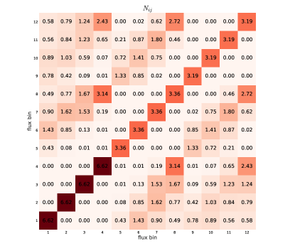
Figure 1: The shot noise matrix $N_{ij}\equiv\frac{\bar{n}_{ij}}{\bar{n}_{i}\bar{n}_{j}}$ derived from the galaxy number density of the 12 flux bins/sub-samples, shown for the photo-$z$ bin $0.4<z_{\kappa}<0.6$ as an example. The diagonal elements $N_{ii}\equiv\frac{1}{\bar{n}_{i}}$ are measured from the average number density of each flux bin (the fourth column in Table 1). The off-diagonal elements $N_{ij}$ are measured from the overlap between the sub-samples in terms of the number of galaxies they contain (see the discussion in the caption of Table 1). This overlap arises form the fact that the relative ranking of galaxy brightness varies in different photometry bands.

III Data analysis

We apply our method of lensing reconstruction to the DES Y3 galaxies from the DES Data Release 2 (DR2Abbott et al. (2018)).

III.1 Data

The DES galaxy samples used for lensing reconstruction are created in accordance with the selection criteria outlined in section 2.1 of Yang et al. (2021). Extended imaging objects are required to have been observed at least once in each optical band to ensure reliable photo-$z$ estimation. After removing objects with Galactic latitude $|\mathrm{b}|<25.0^{\circ}$ to avoid high stellar density regions and objects whose fluxes are affected by bright stars, large galaxies, or globular clusters, we obtain the DES Y3 galaxy sample with a sky coverage of $\sim$4800 deg².

For the convergence-shear cross-correlation analysis, we utilize the DES Y3 shear measurements covering the same footprint as the reconstructed convergence map. The detailed shear measurements procedure, along with the estimated $m$ and $c$, are described in Yao et al. (2023). For both the shear and convergence reconstruction galaxies, we employ the photometric redshift based on Zhou et al. (2021). Note that shear measurements require high imaging quality to ensure reliable shape measurements. Consequently, the number of shear galaxies is significantly smaller than that of the convergence reconstruction galaxies (see Fig. 2).

III.2 Reconstruction

To reconstruct the convergence map, we consider three photometric redshift bins: $0.4<z_{\kappa}<0.6$, $0.6<z_{\kappa}<0.8$, and $0.8<z_{\kappa}<1.0$, selected from the DES Y3 galaxies. As an approximation for the flux-limit selection, for each band, we select galaxies with a magnitude cut approximately 0.5 lower than the peak of the galaxy number counts as a function of magnitude. We then divide the galaxies in each band uniformly into $N_{F}=4$ flux bins, resulting in a total of 12 flux bins at each redshift. For each flux bin, we convert the 3D galaxy number density distribution into a 2D sky map at a resolution of $N_{\rm side}=4096$. We then downgrade the resolution to $N_{\rm side}=1024$ and define the coverage fraction parameter $f_{\beta}$ for each pixel. Pixels with $f_{\beta}$ exceeding the threshold $f=0.9$ are selected. The $f_{\beta}$ definition, steps of measuring galaxy number overdensity, and calculation of the $\alpha$, $g$, $w$ factors for each flux bin are described in Qin et al. (2023). A summary of the flux bins and the results of the $\alpha$, $g$, and $w$ is presented in Table 1. The measured shot noise matrix $N_{ij}\equiv\frac{\bar{n}_{ij}}{\bar{n}_{i}\bar{n}_{j}}$ for $0.4<z_{p}<0.6$ is shown as an example in Fig.1. The reconstructed convergence maps are then obtained by performing a weighted sum over the galaxy overdensity maps (Eq.(4)). For consistency tests described in Sec.IV.1.2 , we also utilize additional sets of magnitude cuts, $N_{F}$, and $f^{\rm threshold}$.

Following Qin et al. (2023); Xu et al. (2023), we mitigate imaging systematics, such as stellar contamination and Galactic extinction, in the reconstructed convergence $\hat{\kappa}$ maps using the Random Forest (RF) mitigation method developed by Chaussidon et al. (2021). The effects of this mitigation on the measured lensing correlation functions are detailed in Appendix A.

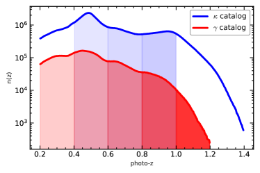
Figure 2: The photometric redshift distributions of the DES Y3 galaxies used for lensing reconstruction (blue line) and the DES Y3 galaxies with shear measurement (red line). The blue shaded regions denote photo-$z$ ranges $0.4<z_{\kappa}<0.6$, $0.6<z_{\kappa}<0.8$, and $0.8<z_{\kappa}<1.0$ employed for lensing reconstruction in our study. The red shaded regions represent the photo-$z$ bins of the shear catalog, [0.2, 0.4, 0.6, 0.8, 1.0, 1.2], defined for cross-correlation analysis. From this figure, we can see that there are many more galaxies available for lensing magnification reconstruction than for cosmic shear measurements.

III.3 Correlation functions

To validate the reconstruction, we analyze the $\hat{\kappa}-\gamma$ and $\hat{\kappa}-\hat{\kappa}$ correlation functions. We select shear galaxies within the photometric redshift range $0.2<z_{\gamma}<1.2$, resulting in about 18 million galaxy shear samples. They are then divided into five photo-$z$ bins: [0.2, 0.4, 0.6, 0.8, 1.0, 1.2]. For each photo-$z$ bin of $\hat{\kappa}$ and $\gamma$, the correlation functions is estimated as follows:

$$\hat{\xi}_{ij}^{\kappa\gamma}(\theta)=\langle\hat{\kappa}_{i}\gamma_{t,j}\rangle_{\theta}/(1+\bar{m})\ .$$ (18)

$$\hat{\xi}^{\kappa\kappa}_{ij}(\theta)=\langle\hat{\kappa}_{i}\hat{\kappa}_{j}\rangle_{\theta}\ .$$ (19)

Here, the average $\langle\cdots\rangle_{\theta}$ is done over all pixel-galaxy pairs within the angular separation $\theta$, $\bar{m}$ represents the average shear multiplicative bias, and $\gamma_{t}$ is the tangential component of the shear.

For both the convergence-shear and convergence-convergence correlation functions, the calculations are performed using the publicly available code TreeCorr. We use $N=100$ Jackknife patches to estimate the covariance matrix and rescale the covariance matrix following Percival et al. (2014); Wang et al. (2020) to obtain an unbiased estimation.

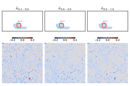
Figure 3: The reconstructed lensing convergence maps. The columns from left to right represent the three photo-$z$ bins of the convergence. The lower panels correspond to zoomed-in views of the areas indicated by the red box in the upper panels. The resolution is downgraded from $N_{\rm side}=1024$ to $N_{\rm side}=256$ for clearer demonstration of the lensing features.

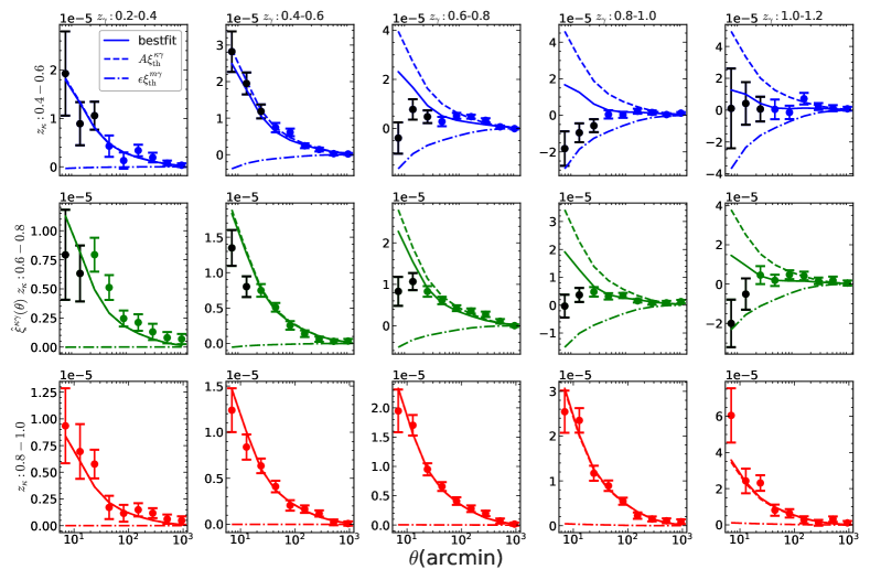
Figure 4: Measured cross correlation function between the reconstructed lensing convergence and the shear. The panels display the results for the three photo-$z$ bins of the convergence from top to bottom, and for the five photo-$z$ bins of the shear from left to right. The blue solid lines represent the best-fit to the model (Eq.(11)). The dashed lines indicate the two components of the best-fit, the signal term $A\xi^{\kappa\gamma}$ and the intrinsic clustering term $\epsilon\xi^{m\gamma}$. Parameters $A$ and $\epsilon$ are defined to quantify the quality of the lensing reconstruction (Eq.(9)). During the fitting, they are kept same across the shear redshift bins. For clarity, only results after the imaging systematics mitigation are shown here. Comparisons of measurements before and after mitigation are shown in Fig.8, while fitting results are summarized in Table 2.

For theoretical calculation of $\xi^{\kappa\gamma}$, $\xi^{m\gamma}$, $\xi^{\kappa_{i}\kappa_{j}}$, $\xi^{m_{i}m_{j}}$, $\xi^{\kappa_{i}m_{j}}$ and $\xi^{\kappa_{j}m_{i}}$, we apply the Core Cosmology Library (CCL, Chisari et al. 2019) and use HaloFit (Smith et al., 2003; Takahashi et al., 2012; Mead et al., 2015) to calculate the nonlinear matter power spectrum. The galaxy redshift distribution $n(z)$ are calculated for each tomographic bin, combining the photo-$z$ distribution and a Gaussian photo-$z$ error PDF with $\sigma_{z}=0.05$. Fig.2 displays the photo-$z$ distribution of the DES Y3 galaxies used for lensing construction and the DES shear catalog. The differences in the theoretical templates’ shape and redshift dependence allow us to separate the measured correlations into the signal term ($\xi^{\kappa\gamma}$ or $\xi^{\kappa\kappa}$) and the intrinsic clustering term ($\xi^{m\gamma}$, $\xi^{mm}$, or $\xi^{\kappa m}$).

		$A$	$\epsilon$	$\chi^{2}_{\rm min}$	$\sqrt{\chi^{2}_{\rm null}-\chi^{2}_{\rm min}}$	$A/\sigma_{A}$	$\rho=\frac{\sigma_{A\epsilon}}{\sqrt{\sigma_{A}\sigma_{\epsilon}}}$
$0.4<z_{\kappa}<0.6$	baseline	3.24$\pm$0.36(3.96$\pm$0.44)	-0.09$\pm$0.02(-0.13$\pm$0.02)	35.2(41.6)	10.5(10.3)	9.0(9.0)	0.8(0.9)
	f=0.5	3.49$\pm$0.34(4.07$\pm$0.44)	-0.10$\pm$0.02(-0.13$\pm$0.02)	33.0(33.3)	11.6(10.4)	10.3(9.2)	0.8(0.9)
	f=0.7	3.58$\pm$0.36(4.09$\pm$0.44)	-0.11$\pm$0.02(-0.14$\pm$0.03)	36.5(30.2)	11.7(10.3)	9.9(9.3)	0.8(0.8)
	$N_{F}=3$	3.88$\pm$0.39(4.31$\pm$0.48)	-0.12$\pm$0.02(-0.15$\pm$0.03)	44.1(35.4)	11.5(10.0)	9.9(9.0)	0.8(0.9)
	$N_{F}=5$	3.25$\pm$0.32(3.94$\pm$0.41)	-0.10$\pm$0.02(-0.12$\pm$0.02)	39.3(36.6)	11.8(11.2)	10.2(9.6)	0.8(0.9)
	$m_{g,r,z}-0.5$	2.95$\pm$0.33(3.13$\pm$0.42)	-0.07$\pm$0.02(-0.08$\pm$0.02)	35.7(33.5)	11.0(9.3)	8.9(7.5)	0.8(0.8)
	$m_{g}-0.5$	3.45$\pm$0.35(3.98$\pm$0.40)	-0.10$\pm$0.02(-0.13$\pm$0.02)	33.2(32.5)	11.3(11.4)	9.9(9.9)	0.8(0.8)
	$m_{r}-0.5$	3.02$\pm$0.33(3.27$\pm$0.40)	-0.07$\pm$0.02(-0.08$\pm$0.02)	44.9(38.3)	11.8(10.0)	9.2(8.2)	0.8(0.8)
	$m_{z}-0.5$	3.59$\pm$0.37(3.96$\pm$0.44)	-0.11$\pm$0.02(-0.13$\pm$0.02)	34.2(29.7)	11.3(10.2)	9.7(9.0)	0.8(0.9)
$0.6<z_{\kappa}<0.8$	baseline	1.76$\pm$0.11(1.93$\pm$0.13)	-0.10$\pm$0.02(-0.12$\pm$0.02)	36.5(33.5)	18.4(17.4)	16.0(14.8)	0.7(0.8)
	f=0.5	1.75$\pm$0.12(1.87$\pm$0.13)	-0.10$\pm$0.02(-0.11$\pm$0.02)	38.9(33.8)	17.6(16.9)	14.6(14.4)	0.7(0.8)
	f=0.7	1.76$\pm$0.11(1.86$\pm$0.13)	-0.10$\pm$0.02(-0.11$\pm$0.02)	40.2(34.0)	18.3(16.9)	16.0(14.3)	0.7(0.8)
	$N_{F}=3$	1.75$\pm$0.11(1.87$\pm$0.13)	-0.11$\pm$0.02(-0.12$\pm$0.02)	38.5(36.1)	17.6(16.3)	15.9(14.4)	0.7(0.8)
	$N_{F}=5$	1.74$\pm$0.11(1.85$\pm$0.13)	-0.09$\pm$0.02(-0.10$\pm$0.02)	41.3(35.9)	19.1(17.7)	15.8(14.2)	0.7(0.8)
	$m_{g,r,z}-0.5$	1.95$\pm$0.13(2.06$\pm$0.15)	-0.09$\pm$0.02(-0.09$\pm$0.02)	36.2(30.7)	18.4(16.8)	15.0(13.7)	0.7(0.8)
	$m_{g}-0.5$	1.90$\pm$0.12(2.08$\pm$0.14)	-0.11$\pm$0.02(-0.14$\pm$0.02)	35.7(34.9)	18.7(17.2)	15.8(14.9)	0.7(0.8)
	$m_{r}-0.5$	1.60$\pm$0.12(1.72$\pm$0.14)	-0.08$\pm$0.02(-0.09$\pm$0.02)	32.9(31.8)	15.7(14.8)	13.3(12.3)	0.8(0.8)
	$m_{z}-0.5$	2.17$\pm$0.13(2.37$\pm$0.15)	-0.10$\pm$0.02(-0.11$\pm$0.02)	41.2(31.4)	20.4(19.8)	16.7(15.8)	0.8(0.8)
$0.8<z_{\kappa}<1.0$	baseline	1.19$\pm$0.06(1.17$\pm$0.07)	0.01$\pm$0.04(0.06$\pm$0.04)	26.5(41.8)	28.4(23.4)	19.8(16.8)	0.7(0.7)
	f=0.5	1.20$\pm$0.06(1.18$\pm$0.06)	0.02$\pm$0.05(0.02$\pm$0.05)	25.1(40.3)	27.2(28.0)	20.0(19.7)	0.7(0.7)
	f=0.7	1.18$\pm$0.05(1.18$\pm$0.05)	0.02$\pm$0.04(0.05$\pm$0.04)	24.0(39.2)	28.8(29.4)	23.6(23.6)	0.6(0.6)
	$N_{F}=3$	1.28$\pm$0.05(1.26$\pm$0.05)	-0.01$\pm$0.05(0.03$\pm$0.04)	22.5(37.7)	29.1(31.7)	25.6(25.2)	0.6(0.6)
	$N_{F}=5$	1.17$\pm$0.05(1.16$\pm$0.06)	0.00$\pm$0.04(0.04$\pm$0.04)	24.7(42.8)	28.6(29.6)	23.4(19.3)	0.6(0.7)
	$m_{g,r,z}-0.5$	0.97$\pm$0.06(0.96$\pm$0.06)	-0.02$\pm$0.05(0.02$\pm$0.04)	26.8(42.1)	21.5(22.1)	16.2(16.0)	0.6(0.6)
	$m_{g}-0.5$	1.21$\pm$0.06(1.19$\pm$0.05)	0.01$\pm$0.04(0.05$\pm$0.04)	26.3(41.8)	28.0(30.1)	20.2(23.8)	0.6(0.6)
	$m_{r}-0.5$	1.15$\pm$0.06(1.13$\pm$0.05)	-0.03$\pm$0.05(0.00$\pm$0.04)	25.1(46.4)	25.6(27.3)	19.2(22.6)	0.6(0.7)
	$m_{z}-0.5$	0.96$\pm$0.06(0.96$\pm$0.06)	0.02$\pm$0.05(0.05$\pm$0.05)	29.2(44.4)	21.0(21.8)	16.0(16.0)	0.7(0.7)

Table 2: Results of the convergence-shear cross-correlation analysis for the three photo-$z$ bins of convergence. Besides the baseline, the impacts of $f^{\rm threshold},N_{F}$, the three bands magnitude cuts on the analysis are tested. The baseline sets are $f^{\rm threshold}=0.9,N_{F}=4$ and magnitude cuts shown in Table 1. The results are presented from top to bottom for the photo-$z$ bins $0.4<z_{\kappa}<0.6$, $0.6<z_{\kappa}<0.8$, and $0.8<z_{\kappa}<1.0$. And the d.o.f. = 28, 33, and 43 for the three $z_{\kappa}$ bins, respectively. The fitting results remain consistent across different $f^{\rm threshold}$, $N_{F}$, and magnitude cuts. The main table shows the results after the mitigation, while in parentheses are the results before the mitigation. The $S/N$ of the detection of the weak lensing signal is enhanced after the mitigation. The last column shows the correlation coefficient between $A$ and $\epsilon$, where $\sigma^{2}_{A\epsilon}$, $\sigma^{2}_{A}$, and $\sigma^{2}_{\epsilon}$ are the (co)variances.

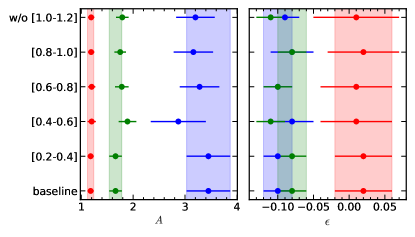
Figure 5: Impact of the shear redshifts on the constraints of $A$ (the left panel) and $\epsilon$ (the right panel). We drop one shear redshift bin at a time, and perform the cross correlation analysis and constrain the parameters with the remaining bins. The y-axis denote the shear redshift bin that is dropped. The shadow regions shows the $1\sigma$ error of the constraints for the baseline set (i.e., all the shear bins are included). The colors red, green, and blue indicate the convergence map reconstructed in the photo-$z$ bins $0.4<z_{\kappa}<0.6$, $0.6<z_{\kappa}<0.8$, and $0.8<z_{\kappa}<1.0$, respectively. The constraining results are consistent with the baseline set for all the cases, which indicates the robustness of the cross-correction analysis against different shear samples.

	baseline	A=0	A=1	$\epsilon$=0
$\chi^{2}_{\rm min}$	35.2	117.5	81.1	61.2
AIC	39.3	119.5	83.2	63.3
$\chi^{2}_{\rm min}$	36.5	286.9	83.2	67.5
AIC	40.6	288.9	85.3	69.6
$\chi^{2}_{\rm min}$	26.5	483.1	38.1	26.6
AIC	30.6	485.2	40.1	28.6

Table 3: Akaike Information Criterion (AIC) Results for Convergence-Shear Cross-Correlation Analysis. The baseline model follows Eq. (11). Other models set $A=0$, $A=1$, or $\epsilon=0$. Results, from top to bottom, correspond to lensing convergence in photo-$z$ bins: $0.4<z_{\kappa}<0.6$, $0.6<z_{\kappa}<0.8$, and $0.8<z_{\kappa}<1.0$. In all cases, except where $\epsilon=0$ for $0.8<z_{\kappa}<1.0$, alternative models are ruled out, with AIC scores exceeding the baseline by more than 10. This suggests the robustness of the weak lensing signal detection and the minimal residual galaxy clustering contamination for $0.8<z_{\kappa}<1.0$.

IV Results

We present visualizations of the reconstructed convergence maps of the three $z_{\kappa}$ bins in Fig.3. The maps reveal lensing features of the large-scale structure. We analyze the derived correlation functions from these maps to validate the lensing reconstruction.

IV.1 Convergence-shear cross correlation

IV.1.1 Baseline results

Figure 4 displays the measured convergence-shear cross-correlation $\hat{\xi}^{\kappa\gamma}$. Significant cross-correlation signals are detected for the convergence maps reconstructed in the three photo-$z$ bins, spanning the five photo-$z$ bins of the shear. For each photo-$z$ bin of the convergence, we fit the cross-correlation measurements to the theoretical model (Eq. (11)), keeping $A$ and $\epsilon$ fixed across the shear redshift bins. For map $\hat{\kappa}_{i}$, the $\chi^{2}$ for the fitting is approximated by

$$\chi^{2} \approx\sum\limits_{j\alpha\beta}\big{[}\hat{\xi}^{\kappa\gamma}_{j}(\theta_{\alpha})-{\xi}^{\kappa\gamma}_{j,\rm th}(\theta_{\alpha})\big{]}\times\textbf{Cov}_{j}^{-1}$$ (20)

$$\times\big{[}\hat{\xi}^{\kappa\gamma}_{j}(\theta_{\beta})-{\xi}^{\kappa\gamma}_{j,\rm th}(\theta_{\beta})\big{]}\ .$$

Here, Cov is the data covariance matrix.

The best fit is

$$\big{(}A^{\text{bestfit}}\ \epsilon^{\text{bestfit}}\big{)}^{\mathbf{T}}=\bm{F}^{-1}\bigg{[}\sum_{j}\bm{\xi}_{j}^{\mathbf{T}}\textbf{Cov}_{j}^{-1}\bm{\hat{\xi}}_{j}\bigg{]}\ ,$$ (21)

where

$$\bm{\xi}_{j}\equiv\begin{pmatrix}\xi_{j,{\rm th}}^{\kappa\gamma}(\theta_{1})&\xi_{j,{\rm th}}^{\kappa m}(\theta_{1})\\ \xi_{j,{\rm th}}^{\kappa\gamma}(\theta_{2})&\xi_{j,{\rm th}}^{\kappa m}(\theta_{2})\\ \vdots&\vdots\\ \xi_{j,{\rm th}}^{\kappa\gamma}(\theta_{n})&\xi_{j,{\rm th}}^{\kappa m}(\theta_{n})\end{pmatrix};\ \ \hat{\bm{\xi}}_{j}\equiv\begin{pmatrix}\hat{\xi}_{j}^{\kappa\gamma}(\theta_{1})\\ \hat{\xi}_{j}^{\kappa\gamma}(\theta_{2})\\ \vdots\\ \hat{\xi}_{j}^{\kappa\gamma}(\theta_{n})\end{pmatrix}\ .$$ (22)

$\bm{F}$ is the fisher matrix of $A$ and $\epsilon$,

$$\bm{F}= \begin{pmatrix}\sum\limits_{j\alpha\beta}\xi^{\kappa\gamma}_{j,\alpha}\textbf{Cov}_{j}^{-1}\xi^{\kappa\gamma}_{j,\beta}&\sum\limits_{j\alpha\beta}\xi^{\kappa\gamma}_{j,\alpha}\textbf{Cov}_{j}^{-1}\xi^{\kappa m}_{j,\beta}\\ \sum\limits_{j\alpha\beta}\xi^{\kappa\gamma}_{j,\alpha}\textbf{Cov}_{j}^{-1}\xi^{\kappa m}_{j,\beta}&\sum\limits_{j\alpha\beta}\xi^{\kappa m}_{j,\alpha}\textbf{Cov}_{j}^{-1}\xi^{\kappa m}_{j,\beta}\end{pmatrix}\$$

The associated errors and covariance matrix of the constraints are given by $\bm{F}^{-1}$.

We use $\chi^{2}_{\rm min}$ and ${\chi^{2}_{\rm null}}$to demonstrate the goodness of fit to the model, where the $\chi^{2}_{\rm null}$ and $\chi^{2}_{\rm min}$ is defined by

$$\chi^{2}_{\rm null}=\sum\limits_{j\alpha\beta}\big{[}\hat{\xi}^{\kappa\gamma}_{j}(\theta_{\alpha})\big{]}\textbf{Cov}_{j}^{-1}\big{[}\hat{\xi}^{\kappa\gamma}_{j}(\theta_{\beta})\big{]}\ ,$$ (23)

$$\chi^{2}_{\rm min} =\sum\limits_{j\alpha\beta}\big{[}\hat{\xi}^{\kappa\gamma}_{j}(\theta_{\alpha})-{\xi}_{j,\rm th}^{\rm bestfit}(\theta_{\alpha})\big{]}\times\textbf{Cov}_{j}^{-1}$$ (24)

$$\times\big{[}\hat{\xi}^{\kappa\gamma}_{j}(\theta_{\beta})-{\xi}_{j,\rm th}^{\rm bestfit}(\theta_{\beta})\big{]}\ ,$$

where

$$\xi_{\rm th}^{\rm bestfit}=A^{\rm bestfit}\xi^{\kappa\gamma}+\epsilon^{\rm bestfit}\xi^{m\gamma}\ .$$ (25)

To achieve reasonable fitting results / $\chi^{2}_{\rm min}$, we cut the first 3 angular bins of the $\langle\hat{\kappa}\gamma\rangle$ measurements for $0.4<z_{\kappa}<0.6$ and the first 2 for $0.6<z_{\kappa}<0.8$. These small scales are expected to be affected by factors such as the baryonic feedback, which are not adequately captured by our model. We leave the investigation of these scales to future studies. Note that, for the joint analysis of convergence-convergence and convergence-shear presented in Appendix B, we use the same scale cuts.

Table 2 summarizes the fitting results. The degrees of freedom ($\mathrm{d.o.f.}$) for the fitting are 28, 33, and 43 for the convergence maps at $0.4<z_{\kappa}<0.6$, $0.6<z_{\kappa}<0.8$, and $0.8<z_{\kappa}<1.0$, respectively. The two-parameter fitting returns a reasonable $\chi^{2}_{\rm min}/\mathrm{d.o.f.}\sim 1$, supporting our theoretical modeling.

According to $A$, we detect a convergence-shear cross-correlation signal with $S/N\equiv A/\sigma_{A}\gtrsim 10$ for the three convergence maps. The $S/N$ reaches 20 for the convergence map at $0.8<z_{\kappa}<1.0$. Deviation from one is detected in $A$ and increases as the redshift decreases, starting from $A\sim 1.2$ for $0.8<z_{\kappa}<1.0$ and reaching $\sim 3$ for $0.4<z_{\kappa}<0.6$. This tendency is consistent with the results of our reconstruction for the DECaLS galaxies (Qin et al., 2023), where $A$ is found to be $\sim 0.9$ for $0.9<z_{\kappa}<1.2$ and $\sim 2.5$ for $0.5<z_{\kappa}<0.8$. Why $A\neq 1$ and why $A$ has such a redshift dependence are certainly key issues for future investigation.

According to $\epsilon$, galaxy intrinsic clustering is suppressed by a factor of approximately 10 to 100, reaching levels of $\sim-0.10\pm 0.02$ for $0.4<z_{\kappa}<0.6$ and $0.6<z_{\kappa}<0.8$, and $-0.01\pm 0.04$ for $0.8<z_{\kappa}<1.0$. The best-fit to the cross-correlation measurements is shown in Fig.4, with the two components $A\xi^{\kappa\gamma}$ and $\epsilon\xi^{m\gamma}$ also highlighted. The intrinsic clustering term $\epsilon\xi^{m\gamma}$ is negligible for $z_{\kappa}>z_{\gamma}$ (the lower left panels of Fig.4) and becomes significant for $z_{\kappa}<z_{\gamma}$ (the upper right panels of Fig.4). This pattern matches the behavior of the theoretical templates, where matter only correlates with shear when it is at a lower redshift than the shear galaxies. However, our reconstruction suppresses the average galaxy intrinsic clustering, resulting in a small $\epsilon$, thereby suppressing $\epsilon\xi^{m\gamma}$. This makes the signal term $A\xi^{\kappa\gamma}$ the dominant term in the measured cross-correlations.

With non-independent data points and reasonable covariance estimation, $\chi^{2}_{\rm null}=145.2,375.0,833.1$ and $\chi^{2}_{\min}=35.2,36.5,26.5$ with respect to the null and to the model, respectively. According to the data-driven signal-to-noise ratio $\sqrt{\chi^{2}_{\rm null}}$, we achieve $12.0\sigma,19.4\sigma,28.9\sigma$ detection of non-zero cross-correlation signals for the three photo-$z$ bins of $\hat{\kappa}$. Based on the fitting-driven signal-to-noise ratio $\sqrt{\chi^{2}_{\rm null}-\chi^{2}_{\rm min}}$, the significance is approximately $10.5\sigma,18.4\sigma,28.4\sigma$. The lensing signal is detected at lower significance ($A/\sigma_{A}=9,16,20$). Table 2 also compares results before and after imaging systematics mitigation, showing consistency in the fitting results. After mitigation, both $\sqrt{\chi^{2}_{\rm null}-\chi^{2}_{\rm min}}$ and $A/\sigma_{A}$ exhibit increases.

IV.1.2 Internal test of the convergence-shear cross-correlation analysis

We evaluate the influence of various factors in our analysis, as presented in Table 2- 3 and Fig.5

• Impact of $f^{\rm threshold}$. A higher $f^{\rm threshold}$ implies a stricter selection of pixels in the galaxy number overdensity map. Table 2 indicates that the effect of $f^{\rm threshold}$ is minimal, and the fitting results remain consistent across $f^{\rm threshold}=0.5,0.7,0.9$.

• Impact of $N_{F}$. The constraints on $A$ and $\epsilon$ are stable across $N_{F}=3,4,5$. The parameter $\epsilon=\Sigma_{i}w_{i}b_{i}$ depends on the galaxy biases in the chosen flux bins and, consequently, on the number of flux bins $N_{F}$. The stability of $\epsilon$ across different $N_{F}$ values suggests that our method for eliminating galaxy intrinsic clustering is robust.

• Impact of the magnitude cut. We select galaxies that are 0.5 magnitudes brighter than the baseline set. The first scenario involves selecting galaxies that are 0.5 magnitudes brighter across all three bands, denoted as $m_{g,r,z}-0.5$. The other three scenarios involve selecting galaxies that are 0.5 magnitudes brighter in each band individually, denoted as $m_{g}-0.5$, $m_{r}-0.5$, and $m_{z}-0.5$. A brighter magnitude cut of 0.5 results in a reduction of approximately 30$-$40% in the number of galaxies for a particular photometry band. Consequently, the $S/N$ of the cross-correlation signal is reduced for a brighter magnitude cut. Nevertheless, the constraints on $A$ and $\epsilon$ remain stable across different magnitude cuts, as shown in Table 2.

• Impact of imaging systematics. Since they are unlikely to cause density fluctuations correlated with cosmic shear, their main impact is to introduce spurious fluctuations from contamination such as stellar density, Galactic extinction, sky brightness, seeing, and airmass. Table 2 shows that the fitting results are consistent before and after the mitigation. However errorbars in $A$ and $\epsilon$ shrink after the mitigation.

• Impact of the shear catalog. Since parameters $A$ and $\epsilon$ characterize the reconstructed lensing convergence, they should be independent of the shear catalog used. We investigate the impact of selecting different shear catalogs by systematically excluding one shear photo-$z$ bin at a time. The results are presented in Fig. 5. For all the investigated cases, the constraints on $A$ and $\epsilon$ align with the baseline set within the $1\sigma$ error range, indicating the robustness of the analysis against different shear samples.

• Akaike information criterion (AIC) analysis. We adjust the theoretical template to compare different models. Besides the baseline model described by Eq. (11), we also consider alternative models where either $A$ or $\epsilon$ is fixed. We compare four scenarios: the baseline model, fixing $A=0$, fixing $A=1$, and fixing $\epsilon=0$. For each model, we repeat the fitting process and then calculate the AIC, which can be expressed, to second-order, as:

  $$\mathrm{AIC}_{\mathrm{c}}=-2\ln p\left(\lambda_{\text{bestfit }}\mid D\right)+2N_{\lambda}+\frac{2N_{\lambda}+1}{N_{D}-N_{\lambda}-1}.$$

  Here, $N_{\lambda}$ is the number of parameters, $N_{D}$ is the number of data points, $p$ is the likelihood which is Gaussian in our case, and $p\left(\lambda_{\text{bestfit }}\mid D\right)$ is the value for the best-fit parameters. The best model has the smallest AIC. A model with an AIC larger by 10 or more should be ruled out, while a difference of less than 2 suggests the models are indistinguishable. Table 3 shows the results of $\chi^{2}_{\rm min}$ (the minimum $\chi^{2}$ value obtained during fitting) and AIC. In all cases, except where $\epsilon=0$ for $0.8<z_{\kappa}<1.0$, alternative models are ruled out by AIC. This suggests the robustness of the weak lensing signal detection (ruling out $A=0$), the significance of the multiplicative bias in the amplitude of $\hat{\kappa}$ (ruling out $A=1$), and the necessity of the intrinsic clustering term in the model (ruling out $\epsilon=0$).

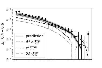
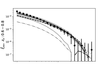
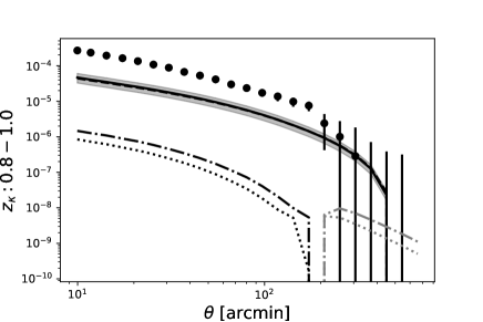
Figure 6: The auto-correlation measurements of the reconstructed lensing convergence and their comparison to the prediction. Three photo-$z$ bins are shown in the three panels. The errors of the measurements are estimated by the jackknife method. The black solid line represents the prediction from the deterministic terms, with parameters $A$ and $\epsilon$ derived from the convergence-shear cross-correlation analysis. The shaded region indicates the 1$\sigma$ error of the prediction, calculated through error propagation of the fitting results for $A$ and $\epsilon$. The three components of the prediction, i.e., the $A^{2}\xi^{\kappa\kappa}$, $\epsilon^{2}\xi^{mm}$, and $2A\epsilon\xi^{m\kappa}$, are shown with dashed, dotted, and dash-dotted lines, respectively. The light-grey lines indicate where the values are negative. For the photo-$z$ bin $0.4<z_{\kappa}<0.6$ and $0.6<z_{\kappa}<0.8$, the predictions match the measurements well. The $A^{2}\xi^{\kappa\kappa}$ term dominates the prediction at large scales, while the $\epsilon^{2}\xi^{mm}$ term dominates at small scales. For the photo-$z$ bin $0.8<z_{\kappa}<1.0$, the measurements are significantly higher than the prediction at all scales. the stochastic term, which are not included in the prediction, are expected to contribute to this discrepancy. For clarity, only the results after the imaging systematics mitigation are shown here. The measurements before/after the imaging systematics mitigation are compared in Fig.9.

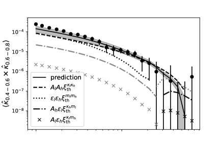
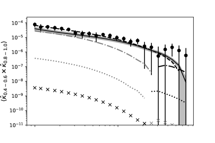
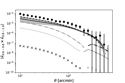
Figure 7: Same as Fig.6, but for the cross-correlation between different photo-$z$ bins of the reconstructed lensing convergence. The three panels show different combinations of the photo-$z$ bins. The prediction consists of four components: $A_{l}A_{h}\xi^{\kappa_{l}\kappa_{h}}$, $\epsilon_{l}\epsilon_{h}\xi^{m_{l}m_{h}}$, $A_{l}\epsilon_{h}\xi^{\kappa_{l}m_{h}}$, and $A_{h}\epsilon_{l}\xi^{\kappa_{h}m_{l}}$, where the indices $l$/$h$ denote the lower/higher redshift bins. The light-grey lines indicate where the values are negative. For the $(0.4<z_{\kappa}<0.6)\times(0.6<z_{\kappa}<0.8)$ case, the predictions match the measurements well, consistent with the auto-correlation results for the two bins. The $A_{l}A_{h}\xi^{\kappa_{l}\kappa_{h}}$ term dominates the prediction at large scales, while the $\epsilon_{l}\epsilon_{h}\xi^{m_{l}m_{h}}$ term becomes important at small scales. For the other two cases, the predictions are systematically lower, which are expected to result from the influence of stochastic terms for $0.8<z_{\kappa}<1.0$. Notably, the discrepancy is smaller than in the auto-correlation for $0.8<z_{\kappa}<1.0$, which aligns with expectations as the deterministic terms perform well for the lower two redshift bins.

IV.2 Convergence-convergence correlations

Fig.6 shows the measured $\hat{\xi}^{\kappa\kappa}_{ij}$ for $i=j$, representing the auto-correlation of the reconstructed lensing convergence. We also compare the measurements with the deterministic terms $\xi^{\rm D}$ (see Eq.(15)) combined with the fitting results of $A$ and $\epsilon$ from the convergence-shear cross-correlation analysis.

For the photo-$z$ bins $0.4<z_{\kappa}<0.6$ and $0.6<z_{\kappa}<0.8$, the deterministic terms align well with the measurements. The lensing term $A^{2}\xi^{\kappa\kappa}$ dominates the prediction at large scales, while the intrinsic clustering term $\epsilon^{2}\xi^{mm}$ becomes more significant at small scales. This implies that the $\hat{\kappa}$ map has sub-dominant contamination from $\kappa^{\rm S}$.

However, for $0.8<z_{\kappa}<1.0$, the measurements exceed the deterministic terms across all scales, indicating the significance of stochastic terms for this bin. Another potential factor for this discrepancy is residual imaging systematics. The mitigation has a more significant impact on the auto-correlation than on the convergence-shear cross-correlation, as detailed in Appendix A.

The measurements of $\hat{\xi}^{\kappa\kappa}_{ij}$ and the comparison with $\xi^{\rm D}$ for $i\neq j$ are shown in Figure 7. For the $(0.4<z_{\kappa}<0.6)\times(0.6<z_{\kappa}<0.8)$ case, predictions align well with measurements. The lensing term $A_{l}A_{h}\xi^{\kappa_{l}\kappa_{h}}$ dominates at large scales, while the intrinsic clustering term $\epsilon_{l}\epsilon_{h}\xi^{m_{l}m_{h}}$ becomes important at small scales. This is consistent with the auto-correlation behavior for the $0.4<z_{\kappa}<0.6$ and $0.6<z_{\kappa}<0.8$ bins, where deterministic terms match measurements. For the $(0.6<z_{\kappa}<0.8)\times(0.8<z_{\kappa}<1.0)$ and $(0.4<z_{\kappa}<0.6)\times(0.8<z_{\kappa}<1.0)$ cases, the measurements are systematically higher than $\xi^{\rm D}$. However, the discrepancy is smaller than in the auto-correlation case for $0.8<z_{\kappa}<1.0$, aligning with expectations, as the bias mainly originates from the ${\kappa}$ map at $0.8<z_{\kappa}<1.0$. Despite the issues in $0.8<z_{\kappa}<1.0$, the $\hat{\kappa}$ map for $0.4<z_{\kappa}<0.6$ and $0.6<z_{\kappa}<0.8$ is shown to have negligible / sub-dominant $\kappa^{\rm S}$.

V SUMMARY and discussion

Using cosmic magnification, we reconstruct the weak lensing convergence maps from the DES Y3 galaxies. It is achieved by weighting the overdensity maps of galaxies across different magnitude bins and photometric bands. To validate the reconstruction, we measure and compare the convergence-shear and convergence-convergence correlations with the theoretical model. The $\hat{\kappa}-\gamma$ analysis indicates that our method effectively eliminates galaxy intrinsic clustering, achieving $\sim 10\sigma$ to $\sim 20\sigma$ detection of the $\hat{\kappa}-\gamma$ cross-correlation signal. The $\hat{\kappa}-\hat{\kappa}$ correlations of the $0.4<z_{\kappa}<0.6$ and $0.6<z_{\kappa}<0.8$ bins show reasonably good agreement with predictions based on theoretical interpretation of $\hat{\kappa}-\gamma$ measurement.

Several issues remain prominent for future improvement. The first is the bias in the overall amplitude of the reconstructed lensing convergence maps. The bias increases as the redshift decreases, with values ranging from $\sim 1.2$ to $\sim 3.2$. The agreement between the convergence-shear and convergence-convergence analyses for the lower two convergence redshift bins indicates that the $\langle\hat{\kappa}\hat{\kappa}\rangle$ measurements also support the existence of the bias (see Appendix B). The amplitude and redshift dependence of the bias are similar to those observed in the reconstructed convergence for the DECaLS galaxies (Qin et al., 2023), where tests suggest that the biases are potentially caused by approximations in the galaxy selection function. This approximation, which treats galaxy selection as flux-limited, is commonly used in cosmic magnification signal detections (e.g., Tudorica et al., 2017; Bonavera et al., 2021; Crespo et al., 2022). Further investigation into the forward modeling (von Wietersheim Kramsta et al., 2021; Elvin-Poole et al., 2023a) of the galaxy selection function is crucial for the effective application of cosmic magnification in weak lensing studies. Another issue is the discrepancy observed in the $\hat{\kappa}-\hat{\kappa}$ measurements of the $0.8<z_{\kappa}<1.0$ bin. A better understanding of galaxy stochasticity (e.g., Zhou and Zhang, 2024a; Tegmark and Bromley, 1999; Bonoli and Pen, 2009b) is needed to address this discrepancy.

Another existing dataset suitable for our reconstruction method is the HSC (Aihara et al., 2018) survey, which has a depth $\sim 2$ magnitude deeper than DES. It is expected that the magnification signal, especially the $\hat{\kappa}-\hat{\kappa}$ correlations, from HSC will be further improved. This is the next step in our research. By leveraging the DECaLS, DES, and HSC data, along with insights from simulations (Ma et al., 2024; Zhou and Zhang, 2024b), we aim to validate and refine our method, ultimately paving the way for its cosmological application to future, even deeper surveys like LSST (LSST, LSST Science Collaboration et al., 2009), Euclid (Laureijs et al., 2011) and CSST (Gong et al., 2019).

Appendix A The imaging systematics mitigation on the measured correction functions

Fig.8 shows the measured convergence-shear cross-correlation function before and after mitigating imaging systematics. The impact of this mitigation on the convergence-shear cross-correlation is minor. The reconstruction of the convergence relies on galaxy luminosity, while the shear is measured from galaxy shapes. As a result, they are sensitive to different imaging systematics, which explains the minor impact observed.

The convergence-convergence corrections are shown in Fig.9. In all cases, mitigating imaging systematics significantly reduces the amplitude of the measurements. The galaxy luminosity at two photo-$z$ bins is sensitive to the same imaging systematics. Therefore, unlike the convergence-shear correlation, the cross-correlation between these bins cannot efficiently eliminate the systematics. The discrepancy between the measurements and the predictions is significantly reduced after mitigation (Fig.6 and Fig.7).

Appendix B Constraints from ignoring stochastic terms

For the lensing convergence reconstructed at $0.4<z_{\kappa}<0.6$ and $0.6<z_{\kappa}<0.8$, the measured convergence-convergence correlations align well with the predictions. This suggests that, for these redshift bins, the modeling of the convergence-convergence correlations can be approximated using deterministic terms (see Eq.(15))

$${\xi}^{\kappa\kappa}_{ij,\rm th}\approx\xi_{ij}^{\rm D}\ .$$ (26)

Using this approximation, we can establish constraints on the parameters $A$ and $\epsilon$ based solely on convergence-convergence correlations. These constraints can then be compared with results from the convergence-shear cross-correlation analysis. The $\chi^{2}$ for jointly fitting the convergence-convergence (auto- and cross-) correlations of the two convergence maps is approximated by:

$$\chi^{2} \approx\sum_{i\geq j}\sum\limits_{j\alpha\beta}\big{[}\hat{\xi}^{\kappa\kappa}_{ij}(\theta_{\alpha})-{\xi}_{ij,\rm th}^{\kappa\kappa}(\theta_{\alpha})\big{]}\times\textbf{Cov}_{ij}^{-1}$$ (27)

$$\times\big{[}\hat{\xi}^{\kappa\kappa}_{ij}(\theta_{\beta})-{\xi}_{ij,\rm th}^{\kappa\kappa}(\theta_{\beta})\big{]}\ .$$

Here the summation over indices $i,j$ contains three terms: $i=j=l$, $i=j=h$, and $i=l,j=h$, corresponding to the auto-correlation of the two convergence maps at $0.4<z_{\kappa}<0.6\ (l)$ and $0.6<z_{\kappa}<0.8\ (h)$, and their cross-correlation. The likelihood for this case is non-Gaussian. To obtain constraints on $A_{l},A_{h},\epsilon_{l},\epsilon_{h}$, we use the publicly available code emcee (Foreman-Mackey et al., 2013) to sample the posterior distribution of the parameters $A$ and $\epsilon$. The results of the posterior and the comparison with constraints from the convergence-shear cross-correlation analysis are shown in Fig.10.

For $A_{l}$ and $\epsilon_{h}$, the discrepancy in constraints between the two analyses is $\lesssim 1\sigma$, whereas for $A_{h}$ and $\epsilon_{l}$, the discrepancy is $\lesssim 2\sigma$. The parameter degeneracy in the $A_{l}-\epsilon_{h}$ and $A_{h}-\epsilon_{l}$ planes differs in direction between the two analyses. This indicates that a joint fitting of the convergence-convergence and convergence-shear correlations can break these degeneracies. The $\chi^{2}$ for the joint fitting is approximated by:

$$\chi^{2} \approx\sum_{i\geq j}\sum\limits_{j\alpha\beta}\big{[}\hat{\xi}^{\kappa\kappa}_{ij}(\theta_{\alpha})-{\xi}_{ij,\rm th}^{\kappa\kappa}(\theta_{\alpha})\big{]}\times\textbf{Cov}_{ij}^{-1}$$ (28)

$$\times\big{[}\hat{\xi}^{\kappa\kappa}_{ij}(\theta_{\beta})-{\xi}_{ij,\rm th}^{\kappa\kappa}(\theta_{\beta})\big{]}$$

$$+\sum\limits_{ij\alpha\beta}\big{[}\hat{\xi}^{\kappa\gamma}_{ij}(\theta_{\alpha})-{\xi}_{ij,\rm th}(\theta_{\alpha})\big{]}\times\textbf{Cov}_{ij}^{-1}$$

$$\times\big{[}\hat{\xi}^{\kappa\gamma}_{ij}(\theta_{\beta})-{\xi}_{ij,\rm th}(\theta_{\beta})\big{]}\ .$$

In the second term of the $\chi^{2}$, the summation over index $i$ encompasses the two convergence maps, while the sum over $j$ covers the shear photo-$z$ bins. As presented in Fig.10, the degeneracy is reduced, and the figure of merit shows improvement compared to analyzing convergence-shear or convergence-convergence alone. This highlights the potential of combining magnification and shear measurements to enhance cosmological constraints. Note that throughout this work, we have neglected correlations between $\xi^{\kappa\kappa}_{ij}$ or $\xi^{\kappa\gamma}_{ij}$ of different convergence or shear redshifts ($i_{1}\neq i_{2},j_{1}\neq j_{2}$) arising from four-point correlations. For the current data, these correlations are negligible compared to the shape measurement error in $\gamma$ and the shot noise in $\kappa$.

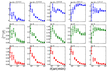
Figure 8: Comparison of the measured convergence-shear cross-correlation before and after the imaging systematics mitigation. The panels display the results for the three photo-$z$ bins of the convergence from top to bottom, and for the five photo-$z$ bins of the shear from left to right. Triangular and circular points indicate measurements before and after addressing imaging systematics, respectively. The differences are too small to be visible in most cases. The convergence-shear cross-correlation is less affected by the imaging systematics than the convergence-convergence correlation.

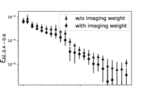
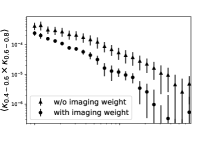
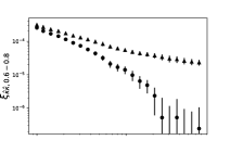
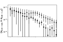
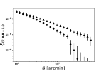
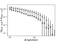
Figure 9: The convergence-convergence correlation measurements of the reconstructed lensing convergence, before and after the imaging systematics mitigation. The left/right panels show the auto-/cross-correlation, while panels from top to bottom display the results for different photo-$z$ bins. The errors of the measurements are estimated by the jackknife method. The triangular/circular data points are the measurements before/after the imaging systematics mitigation. The imaging systematics mitigation significantly reduces the amplitude of the measurements.

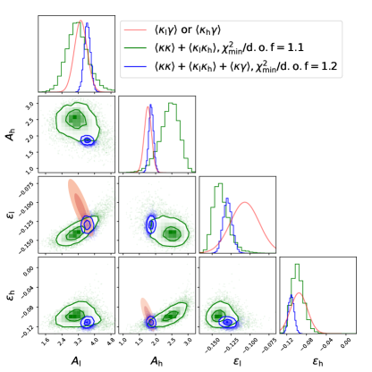
Figure 10: Results of the convergence-convergence correlation analysis for $0.4<z_{\kappa}<0.6$ and $0.6<z_{\kappa}<0.8$. The model for the convergence-convergence correlation is approximated by the deterministic terms. Parameters $A$ and $\epsilon$ are constrained by jointly fitting the auto- and cross-correlations of the two convergence maps, shown by green contours. The indices $l$ and $h$ denote the photo-$z$ bins $0.4<z_{\kappa}<0.6$ and $0.6<z_{\kappa}<0.8$, respectively. As a comparison, the red contours show the fitting results from the convergence-shear cross-correlation analysis (see Sec.IV.1, where only $A_{l}-\epsilon_{l}$ and $A_{h}-\epsilon_{h}$ planes are obtained). The $\lesssim 2\sigma$ discrepancy between the two analyses can be attributed to the approximations in modeling the convergence-convergence correlations. The blue contours shows the constraints obtained by combining the convergence-convergence and convergence-shear cross-correlations. The figure of merit improves compared to analyzing convergence-shear or convergence-convergence alone. The two convergence maps are selected for this analysis, as their convergence-convergence correlations are in good agreement with the predictions from the deterministic terms (see Fig.6 and Fig.7).

References

- Qin et al. (2023) J. Qin, P. Zhang, H. Xu, Y. Yu, J. Yao, R. Ma, and H. Shan, arXiv e-prints arXiv:2310.15053 (2023), eprint 2310.15053.
- Bartelmann and Schneider (2001a) M. Bartelmann and P. Schneider, Phys. Rep. 340, 291 (2001a), eprint astro-ph/9912508.
- Kilbinger (2015a) M. Kilbinger, Reports on Progress in Physics 78, 086901 (2015a), eprint 1411.0115.
- Bartelmann and Schneider (2001b) M. Bartelmann and P. Schneider, Phys. Rep. 340, 291 (2001b), eprint astro-ph/9912508.
- Hoekstra and Jain (2008) H. Hoekstra and B. Jain, Annual Review of Nuclear and Particle Science 58, 99 (2008), eprint 0805.0139.
- Van Waerbeke et al. (2010) L. Van Waerbeke, H. Hildebrandt, J. Ford, and M. Milkeraitis, ApJ 723, L13 (2010), eprint 1004.3793.
- Fu and Fan (2014) L.-P. Fu and Z.-H. Fan, Research in Astronomy and Astrophysics 14, 1061-1120 (2014).
- Kilbinger (2015b) M. Kilbinger, Reports on Progress in Physics 78, 086901 (2015b), eprint 1411.0115.
- Peacock et al. (2006) J. A. Peacock, P. Schneider, G. Efstathiou, J. R. Ellis, B. Leibundgut, S. J. Lilly, and Y. Mellier, ESA-ESO Working Group on “Fundamental Cosmology”, “ESA-ESO Working Group on ”Fundamental Cosmology“, Edited by J.A. Peacock et al. ESA, 2006.” (2006), eprint astro-ph/0610906.
- Albrecht et al. (2006) A. Albrecht, G. Bernstein, R. Cahn, W. L. Freedman, J. Hewitt, W. Hu, J. Huth, M. Kamionkowski, E. W. Kolb, L. Knox, et al., arXiv e-prints astro-ph/0609591 (2006), eprint astro-ph/0609591.
- Dark Energy Survey Collaboration et al. (2016) Dark Energy Survey Collaboration, T. Abbott, F. B. Abdalla, J. Aleksić, S. Allam, A. Amara, D. Bacon, E. Balbinot, M. Banerji, K. Bechtol, et al., MNRAS 460, 1270 (2016), eprint 1601.00329.
- de Jong et al. (2013) J. T. A. de Jong, G. A. Verdoes Kleijn, K. H. Kuijken, and E. A. Valentijn, Experimental Astronomy 35, 25 (2013), eprint 1206.1254.
- Aihara et al. (2018) H. Aihara, N. Arimoto, R. Armstrong, S. Arnouts, N. A. Bahcall, S. Bickerton, J. Bosch, K. Bundy, P. L. Capak, J. H. H. Chan, et al., PASJ 70, S4 (2018), eprint 1704.05858.
- LSST Science Collaboration et al. (2009) LSST Science Collaboration, P. A. Abell, J. Allison, S. F. Anderson, J. R. Andrew, J. R. P. Angel, L. Armus, D. Arnett, S. J. Asztalos, T. S. Axelrod, et al., arXiv e-prints arXiv:0912.0201 (2009), eprint 0912.0201.
- Laureijs et al. (2011) R. Laureijs, J. Amiaux, S. Arduini, J. L. Auguères, J. Brinchmann, R. Cole, M. Cropper, C. Dabin, L. Duvet, A. Ealet, et al., arXiv e-prints arXiv:1110.3193 (2011), eprint 1110.3193.
- Gong et al. (2019) Y. Gong, X. Liu, Y. Cao, X. Chen, Z. Fan, R. Li, X.-D. Li, Z. Li, X. Zhang, and H. Zhan, ApJ 883, 203 (2019), eprint 1901.04634.
- Yao et al. (2024) J. Yao, H. Shan, R. Li, Y. Xu, D. Fan, D. Liu, P. Zhang, Y. Yu, C. Wei, B. Hu, et al., MNRAS 527, 5206 (2024), eprint 2304.04489.
- Hamana et al. (2020) T. Hamana, M. Shirasaki, S. Miyazaki, C. Hikage, M. Oguri, S. More, R. Armstrong, A. Leauthaud, R. Mandelbaum, H. Miyatake, et al., PASJ 72, 16 (2020), eprint 1906.06041.
- Asgari et al. (2021) M. Asgari, C.-A. Lin, B. Joachimi, B. Giblin, C. Heymans, H. Hildebrandt, A. Kannawadi, B. Stölzner, T. Tröster, J. L. van den Busch, et al., A&A 645, A104 (2021), eprint 2007.15633.
- Giblin et al. (2021) B. Giblin, C. Heymans, M. Asgari, H. Hildebrandt, H. Hoekstra, B. Joachimi, A. Kannawadi, K. Kuijken, C.-A. Lin, L. Miller, et al., A&A 645, A105 (2021), eprint 2007.01845.
- Loureiro et al. (2022) A. Loureiro, L. Whittaker, A. Spurio Mancini, B. Joachimi, A. Cuceu, M. Asgari, B. Stölzner, T. Tröster, A. H. Wright, M. Bilicki, et al., A&A 665, A56 (2022), eprint 2110.06947.
- Amon et al. (2022) A. Amon, D. Gruen, M. A. Troxel, N. MacCrann, S. Dodelson, A. Choi, C. Doux, L. F. Secco, S. Samuroff, E. Krause, et al. (DES Collaboration), Phys. Rev. D 105, 023514 (2022), URL https://link.aps.org/doi/10.1103/PhysRevD.105.023514.
- Secco et al. (2022) L. F. Secco, S. Samuroff, E. Krause, B. Jain, J. Blazek, M. Raveri, A. Campos, A. Amon, A. Chen, C. Doux, et al. (DES Collaboration), Phys. Rev. D 105, 023515 (2022), URL https://link.aps.org/doi/10.1103/PhysRevD.105.023515.
- Li et al. (2023) X. Li, T. Zhang, S. Sugiyama, R. Dalal, M. M. Rau, R. Mandelbaum, M. Takada, S. More, M. A. Strauss, H. Miyatake, et al., arXiv e-prints arXiv:2304.00702 (2023), eprint 2304.00702.
- Blandford and Narayan (1992) R. D. Blandford and R. Narayan, ARA&A 30, 311 (1992).
- Bartelmann and Narayan (1995) M. Bartelmann and R. Narayan, in Dark Matter, edited by S. S. Holt and C. L. Bennett (1995), vol. 336 of American Institute of Physics Conference Series, pp. 307–319, eprint astro-ph/9411033.
- Ménard et al. (2010) B. Ménard, R. Scranton, M. Fukugita, and G. Richards, MNRAS 405, 1025 (2010), eprint 0902.4240.
- Jain and Lima (2011) B. Jain and M. Lima, MNRAS 411, 2113 (2011), eprint 1003.6127.
- Schmidt et al. (2012) F. Schmidt, A. Leauthaud, R. Massey, J. Rhodes, M. R. George, A. M. Koekemoer, A. Finoguenov, and M. Tanaka, The Astrophysical Journal 744, L22 (2012), URL http://dx.doi.org/10.1088/2041-8205/744/2/l22.
- Huff and Graves (2014) E. M. Huff and G. J. Graves, ApJ 780, L16 (2014).
- Duncan et al. (2016) C. A. J. Duncan, C. Heymans, A. F. Heavens, and B. Joachimi, Monthly Notices of the Royal Astronomical Society 457, 764–785 (2016), URL http://dx.doi.org/10.1093/mnras/stw027.
- Garcia-Fernandez et al. (2018) M. Garcia-Fernandez, E. Sanchez, I. Sevilla-Noarbe, E. Suchyta, E. M. Huff, E. Gaztanaga, Aleksić, J. , R. Ponce, F. J. Castander, et al., MNRAS 476, 1071 (2018).
- Bauer et al. (2014) A. H. Bauer, E. Gaztañaga, P. Martí, and R. Miquel, Monthly Notices of the Royal Astronomical Society 440, 3701 (2014), https://academic.oup.com/mnras/article-pdf/440/4/3701/3913172/stu530.pdf, URL https://app.dimensions.ai/details/publication/pub.1059915677.
- Bellagamba et al. (2019) F. Bellagamba, M. Sereno, M. Roncarelli, M. Maturi, M. Radovich, S. Bardelli, E. Puddu, L. Moscardini, F. Getman, H. Hildebrandt, et al., MNRAS 484, 1598 (2019), eprint 1810.02827.
- Chiu et al. (2016) I. Chiu, J. P. Dietrich, J. Mohr, D. E. Applegate, B. A. Benson, L. E. Bleem, M. B. Bayliss, S. Bocquet, J. E. Carlstrom, R. Capasso, et al., MNRAS 457, 3050 (2016), eprint 1510.01745.
- Chiu et al. (2020) I. N. Chiu, K. Umetsu, R. Murata, E. Medezinski, and M. Oguri, MNRAS 495, 428 (2020), eprint 1909.02042.
- Scranton et al. (2005) R. Scranton, B. Ménard, G. T. Richards, R. C. Nichol, A. D. Myers, B. Jain, A. Gray, M. Bartelmann, R. J. Brunner, A. J. Connolly, et al., ApJ 633, 589 (2005), eprint astro-ph/0504510.
- Bauer et al. (2012) A. H. Bauer, C. Baltay, N. Ellman, J. Jerke, D. Rabinowitz, and R. Scalzo, ApJ 749, 56 (2012), eprint 1202.1371.
- Morrison et al. (2012) C. B. Morrison, R. Scranton, B. Ménard, S. J. Schmidt, J. A. Tyson, R. Ryan, A. Choi, and D. M. Wittman, MNRAS 426, 2489 (2012), eprint 1204.2830.
- Tudorica et al. (2017) A. Tudorica, H. Hildebrandt, M. Tewes, H. Hoekstra, C. B. Morrison, A. Muzzin, G. Wilson, H. K. C. Yee, C. Lidman, A. Hicks, et al., A&A 608, A141 (2017), eprint 1710.06431.
- Bonavera et al. (2021) L. Bonavera, M. M. Cueli, J. González-Nuevo, T. Ronconi, M. Migliaccio, A. Lapi, J. M. Casas, and D. Crespo, A&A 656, A99 (2021), eprint 2109.12413.
- Crespo et al. (2022) D. Crespo, J. González-Nuevo, L. Bonavera, M. M. Cueli, J. M. Casas, and E. Goitia, A&A 667, A146 (2022), eprint 2210.17318.
- Liu et al. (2021) X. Liu, D. Liu, Z. Gao, C. Wei, G. Li, L. Fu, T. Futamase, and Z. Fan, Phys. Rev. D 103, 123504 (2021), eprint 2104.13595.
- Yao et al. (2023) J. Yao, H. Shan, P. Zhang, E. Jullo, J.-P. Kneib, Y. Yu, Y. Zu, D. Brooks, A. de la Macorra, P. Doel, et al., MNRAS 524, 6071 (2023), eprint 2301.13434.
- Zhang and Pen (2005) P. Zhang and U.-L. Pen, Phys. Rev. Lett. 95, 241302 (2005), eprint astro-ph/0506740.
- Yang and Zhang (2011) X. Yang and P. Zhang, MNRAS 415, 3485 (2011), eprint 1105.2385.
- Zhang et al. (2019) P. Zhang, J. Zhang, and L. Zhang, MNRAS 484, 1616 (2019).
- Yang et al. (2015) X. Yang, P. Zhang, J. Zhang, and Y. Yu, MNRAS 447, 345 (2015).
- Yang et al. (2017) X. Yang, J. Zhang, Y. Yu, and P. Zhang, ApJ 845, 174 (2017), eprint 1703.01575.
- Zhang et al. (2018) P. Zhang, X. Yang, J. Zhang, and Y. Yu, ApJ 864, 10 (2018), eprint 1807.00443.
- Hou et al. (2021) S.-T. Hou, Y. Yu, and P.-J. Zhang, Research in Astronomy and Astrophysics 21, 247 (2021), eprint 2106.09970.
- Ma et al. (2024) R. Ma, P. Zhang, Y. Yu, and J. Qin, MNRAS 527, 7547 (2024), eprint 2306.15177.
- Bonoli and Pen (2009a) S. Bonoli and U. L. Pen, MNRAS 396, 1610 (2009a), eprint 0810.0273.
- Hamaus et al. (2010) N. Hamaus, U. Seljak, V. Desjacques, R. E. Smith, and T. Baldauf, Phys. Rev. D 82, 043515 (2010), eprint 1004.5377.
- Baldauf et al. (2010) T. Baldauf, R. E. Smith, U. Seljak, and R. Mandelbaum, Phys. Rev. D 81, 063531 (2010), eprint 0911.4973.
- Abbott et al. (2018) T. M. C. Abbott, F. B. Abdalla, S. Allam, A. Amara, J. Annis, J. Asorey, S. Avila, O. Ballester, M. Banerji, W. Barkhouse, et al., ApJS 239, 18 (2018), eprint 1801.03181.
- Scranton et al. (2005) R. Scranton, B. Ménard, G. T. Richards, R. C. Nichol, A. D. Myers, B. Jain, A. Gray, M. Bartelmann, R. J. Brunner, A. J. Connolly, et al., The Astrophysical Journal 633, 589 (2005).
- von Wietersheim Kramsta et al. (2021) M. von Wietersheim Kramsta, B. Joachimi, J. L. van den Busch, C. Heymans, H. Hildebrandt, M. Asgari, T. Tr’oster, S. Unruh, and A. H. Wright, Monthly Notices of the Royal Astronomical Society 504, 1452–1465 (2021), URL http://dx.doi.org/10.1093/mnras/stab1000.
- Elvin-Poole et al. (2023a) J. Elvin-Poole, N. MacCrann, S. Everett, J. Prat, E. S. Rykoff, J. De Vicente, B. Yanny, K. Herner, A. Ferté, E. D. Valentino, et al., Monthly Notices of the Royal Astronomical Society 523, 3649 (2023a), ISSN 0035-8711, eprint https://academic.oup.com/mnras/article-pdf/523/3/3649/50596748/stad1594.pdf, URL https://doi.org/10.1093/mnras/stad1594.
- Elvin-Poole et al. (2023b) J. Elvin-Poole, N. MacCrann, S. Everett, J. Prat, E. S. Rykoff, J. De Vicente, B. Yanny, K. Herner, A. Ferté, E. D. Valentino, et al., Monthly Notices of the Royal Astronomical Society 523, 3649 (2023b), ISSN 0035-8711, eprint https://academic.oup.com/mnras/article-pdf/523/3/3649/50596748/stad1594.pdf, URL https://doi.org/10.1093/mnras/stad1594.
- Wenzl et al. (2024) L. Wenzl, S.-F. Chen, and R. Bean, MNRAS 527, 1760 (2024), eprint 2308.05892.
- Zhou et al. (2023) S. Zhou, P. Zhang, and Z. Chen, MNRAS 523, 5789 (2023), eprint 2304.11540.
- Ma et al. (2023) R. Ma, P. Zhang, Y. Yu, and J. Qin, arXiv e-prints arXiv:2306.15177 (2023), eprint 2306.15177.
- Planck Collaboration et al. (2020) Planck Collaboration, N. Aghanim, Y. Akrami, M. Ashdown, J. Aumont, C. Baccigalupi, M. Ballardini, A. J. Banday, R. B. Barreiro, N. Bartolo, et al., A&A 641, A6 (2020), eprint 1807.06209.
- Limber (1953) D. N. Limber, ApJ 117, 134 (1953).
- Yang et al. (2021) X. Yang, H. Xu, M. He, Y. Gu, A. Katsianis, J. Meng, F. Shi, H. Zou, Y. Zhang, C. Liu, et al., The Astrophysical Journal 909, 143 (2021).
- Zhou et al. (2021) R. Zhou, J. A. Newman, Y.-Y. Mao, A. Meisner, J. Moustakas, A. D. Myers, A. Prakash, A. R. Zentner, D. Brooks, Y. Duan, et al., Monthly Notices of the Royal Astronomical Society 501, 3309 (2021).
- Xu et al. (2023) H. Xu, P. Zhang, H. Peng, Y. Yu, L. Zhang, J. Yao, J. Qin, Z. Sun, M. He, and X. Yang, MNRAS 520, 161 (2023), eprint 2209.03967.
- Chaussidon et al. (2021) E. Chaussidon, C. Yèche, N. Palanque-Delabrouille, A. de Mattia, A. D. Myers, M. Rezaie, A. J. Ross, H.-J. Seo, D. Brooks, E. Gaztañaga, et al., Monthly Notices of the Royal Astronomical Society 509, 3904 (2021), ISSN 0035-8711, eprint https://academic.oup.com/mnras/article-pdf/509/3/3904/41446828/stab3252.pdf, URL https://doi.org/10.1093/mnras/stab3252.
- Percival et al. (2014) W. J. Percival, A. J. Ross, A. G. Sánchez, L. Samushia, A. Burden, R. Crittenden, A. J. Cuesta, M. V. Magana, M. Manera, F. Beutler, et al., Monthly Notices of the Royal Astronomical Society 439, 2531 (2014).
- Wang et al. (2020) Y. Wang, G.-B. Zhao, C. Zhao, O. H. E. Philcox, S. Alam, A. Tamone, A. de Mattia, A. J. Ross, A. Raichoor, E. Burtin, et al., Monthly Notices of the Royal Astronomical Society 498, 3470–3483 (2020), URL http://dx.doi.org/10.1093/mnras/staa2593.
- Chisari et al. (2019) N. E. Chisari, D. Alonso, E. Krause, C. D. Leonard, P. Bull, J. Neveu, A. Villarreal, S. Singh, T. McClintock, J. Ellison, et al., ApJS 242, 2 (2019), eprint 1812.05995.
- Smith et al. (2003) R. E. Smith, J. A. Peacock, A. Jenkins, S. D. M. White, C. S. Frenk, F. R. Pearce, P. A. Thomas, G. Efstathiou, and H. M. P. Couchman, MNRAS 341, 1311 (2003), eprint astro-ph/0207664.
- Takahashi et al. (2012) R. Takahashi, M. Sato, T. Nishimichi, A. Taruya, and M. Oguri, ApJ 761, 152 (2012), eprint 1208.2701.
- Mead et al. (2015) A. J. Mead, J. A. Peacock, C. Heymans, S. Joudaki, and A. F. Heavens, MNRAS 454, 1958 (2015), eprint 1505.07833.
- Zhou and Zhang (2024a) S. Zhou and P. Zhang, arXiv e-prints arXiv:2406.03018 (2024a), eprint 2406.03018.
- Tegmark and Bromley (1999) M. Tegmark and B. C. Bromley, ApJ 518, L69 (1999), eprint astro-ph/9809324.
- Bonoli and Pen (2009b) S. Bonoli and U. L. Pen, MNRAS 396, 1610 (2009b), eprint 0810.0273.
- Zhou and Zhang (2024b) S. Zhou and P. Zhang, Phys. Rev. D 110, 063551 (2024b), eprint 2409.01954.
- Foreman-Mackey et al. (2013) D. Foreman-Mackey, D. W. Hogg, D. Lang, and J. Goodman, PASP 125, 306 (2013), eprint 1202.3665.