A Bayesian Model of Underreporting for Sexual Assault on College Campuses
Abstract
In an effort to quantify and combat sexual assault, US colleges and universities are required to disclose the number of reported sexual assaults on their campuses each year. However, many instances of sexual assault are never reported to authorities, and consequently the number of reported assaults does not fully reflect the true total number of assaults that occurred; the reported values could arise from many combinations of reporting rate and true incidence. In this paper we estimate these underlying quantities via a hierarchical Bayesian model of the reported number of assaults. We use informative priors, based on national crime statistics, to act as a tiebreaker to help distinguish between reporting rates and incidence. We outline a Hamiltonian Monte Carlo (HMC) sampling scheme for posterior inference regarding reporting rates and assault incidence at each school, and apply this method to campus sexual assault data from 2014-2019. Results suggest an increasing trend in reporting rates for the overall college population during this time. However, the extent of underreporting varies widely across schools. That variation has implications for how individual schools should interpret their reported crime statistics.
keywords:
capbtabboxtable[][\FBwidth] \endlocaldefs
and
1 Introduction
Sexual assault on college campuses is a pressing public health concern in the United States, prompting government action such as the 2014 formation of the White House Task Force to Protect Students from Sexual Assault (Obama, 2014) and the ”It’s on us” awareness campaign (Somanader, 2014). Per the Clery Act of 1990, US colleges and universities are required to report annual crime statistics for their campuses and adjacent areas. These crime statistics include the number of reported sexual assaults, but because sexual assault is widely believed to be underreported, these figures do not tell the whole story. The number of reported assaults in the Clery data could arise from many different combinations of reporting rates and true underlying numbers of assaults. Without further assumptions, it is equally plausible that a given school has a large number of assaults and a low reporting rate, or few assaults and a high reporting rate.
To estimate the true incidence and reporting rates of sexual assault in the US college population, we construct a hierarchical Bayesian model of the reported data, together with a Markov Chain Monte Carlo (MCMC) sampling scheme for posterior inference. More generally, underreported count data arises in many disciplines, with applications including criminology (Moreno and Giron, 1998; Fernández-Fontelo et al., 2019) as well as epidemiology (Bailey et al., 2005; Bracher and Held, 2021), traffic safety (Kumara and Chin, 2005; Ma and Li, 2010), and economics (Winkelmann, 1996; Fader and Hardie, 2000). The central challenge in such problems is to disentangle the per-school reporting rate from the true latent counts. This issue can be remedied either through the use of validation data not subject to underreporting, or by using domain knowledge to assign more informative prior distributions to latent variables. In the case of campus sexual assault, fully observed validation data is unavailable, and so we use national crime statistics as a source of external information. The absence of fully observed validation data also has implications for model assessment. Without knowledge of the true total number of assaults, we use predictive checks applied to held-out data to demonstrate the fitted model’s compatibility with the data.
In general, we find that inference for the latent total number of assaults and reporting rate at a given school offer a clearer picture of the campus environment than the reported figures alone. In particular, these estimates can suggest the relative contributions of reporting rate and incidence to year-over-year changes in the reported number of assaults. This is a relevant line of inquiry, given that ex ante an increase in the reported number of assaults could equally be explained by an increase in the reporting rate (a positive outcome, indicating that students are aware of campus support resources) or an increase in the true total number of assaults (a bad outcome).
The remainder of this paper is structured as follows. Section 2 reviews related work, followed by an overview of the dataset in Section 3. The proposed modeling methodology is outlined in Section 4. Section 5 discusses modeling results and insights, and Section 6 offers concluding remarks and directions for future work.
2 Related Literature
There are various perspectives on underreported count data. Some studies consider underreporting as a type of censoring. In this formulation, each observed value is possibly right-censored and has an accompanying latent censoring indicator. de Oliveira, Loschi and Assunção (2017) takes this view and assigns a covariate-dependent prior distribution to the latent censoring indicators, including the censoring indicators as a target for posterior inference.
Underreporting also has conceptual overlap with positive-unlabeled (PU) learning. In PU learning, data consist of labeled positive cases and unlabeled cases which may be positive or negative (Letouzey, Denis and Gilleron, 2000). The recorded number of positive cases is thus a lower bound for the true number of positive cases, which can be viewed as an example of underreporting. The application of PU learning techniques to underreported data is explored in Shanmugam and Pierson (2021) and Wu et al. (2023).
Within the broader literature on underreported count data models, one particular line of work is most relevant to modeling reports of sexual assault. These modeling approaches begin with an assumption that the latent true number of events, , follows a Poisson distribution with rate parameter . It is common to further suppose that each of these -many events may or may not be reported, independently of all others, with reporting probability . The number of reported events , where , is the data value we observe.
Moreno and Giron (1998) articulates the identifiability issue in this setup: marginally, the observed data follow a distribution, so without further constraints or assumptions, one cannot distinguish among the possible pairs with the same product. Moreno and Giron (1998) further demonstrate that placing uninformative prior distributions on and is insufficient to produce useful inference. For instance, the choice of a uniform prior on and a Jaynes (Jaynes, 1968) or Jeffreys (Jeffreys, 1946) prior on results in infinite posterior expectations for and given the observed data. In some research applications this identifiability issue is remedied through the use of validation data not subject to underreporting (Powers, Gerlach and Stamey, 2010; Dvorzak and Wagner, 2016). An alternative approach is to use external information to assign informative prior distributions, as Schmertmann and Gonzaga (2018) and Stoner, Economou and Drummond Marques da Silva (2019) do for the reporting probability. Because external information is available regarding both the incidence and reporting rate of sexual assault, we take this latter approach, choosing informative priors for both components of the model.
Earlier work on underreporting models explored the somewhat simpler case of i.i.d. observations governed by a single reporting probability and incidence parameter (Moreno and Giron, 1998; Fader and Hardie, 2000). In this paper we adopt the more recent extension of works such as Dvorzak and Wagner (2016) and Stoner, Economou and Drummond Marques da Silva (2019), allowing and to vary across units. When modeling and , we introduce school features as covariates to account for demographic differences among schools, as detailed in Section 4.
Posterior distributions for latent variables in this type of underreporting model are generally intractable. However, choosing conditionally conjugate priors for and (Gamma and Beta distributions, respectively) leads to analytic expressions for their marginal posterior distributions (Moreno and Giron, 1998; Fader and Hardie, 2000). Alternatively, MCMC approaches to posterior inference allow greater flexibility in choice of priors in exchange for a greater computational burden. Dvorzak and Wagner (2016) use a bespoke implementation of a Gibbs-style sampler, while Stoner, Economou and Drummond Marques da Silva (2019) use slice sampling. Our paper extends this line of work by demonstrating the viability of gradient-based samplers such as HMC for posterior inference in this model setting.
With respect to the application context, the most relevant work comes from Fernández-Fontelo et al. (2019), who model underreporting of domestic violence complaints across districts in Spain. Unlike the campus sexual assault data, observations in Fernández-Fontelo et al. (2019)’s dataset are dense in the time domain (quarterly for 10 years), motivating the authors to adopt time series methodology.
3 Dataset
The dataset contains 11,369 records for 1,973 US colleges and universities over the 2014-2019 time frame 111Data from 2020 and 2021 are excluded. Because the COVID-19 pandemic significantly disrupted patterns of social interaction, campus sexual assault data from this time are not well described by the same model used for other years., where a “record” consists of the total number of assaults reported at a particular school in one particular calendar year. Schools located in the 50 US states, the District of Columbia, and Puerto Rico are included in this analysis. Annual campus crime statistics are furnished by the US Department of Education’s Office of Postsecondary Education. All schools that receive federal financial aid funding under Title IV of the Higher Education Act of 1965 are required to submit annual campus crime reports. Most schools have records for all six years in this time frame, though 8% appear in fewer years due to schools opening/closing or beginning/ ceasing to participate in Title IV.
School characteristics and demographic data are available through the National Center for Education Statistics (NCES), which publishes comprehensive institutional profile information through its IPEDS database 222 https://nces.ed.gov/ipeds/. Preprocessed data is included in the Supplementary Material; raw data is available publicly and from the corresponding author upon reasonable request. Additional dataset details are included in Appendix A.
We exclude institutions with no degree-granting programs and institutions with no programs classified as ”academic” in nature. We also exclude institutions with no residential housing facilities. For such schools, the school does not represent the students’ community, and we would not reasonably expect students to report sexual assaults to the school.
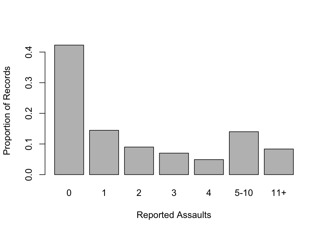
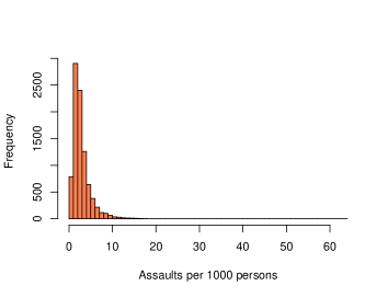
Institutions in this dataset range in size from 5 to 79,500 in-person students, with a median of 2,350. Public institutions comprise 41% of the dataset, religiously affiliated institutions 36%, and private, non-religiously affiliated institutions 22%. The reported sexual assault data is notably sparse: 42% of records show zero reported assaults, and 22% of institutions show no assaults across all six years. The distribution of reported values, shown in Figure 1, has a long right tail, with a handful of schools reporting more than 100 assaults in a given year. This sparsity pattern is not explained by student population size alone: schools with as many as 36,000 students had zero reported assaults, while assaults were reported at schools with as few as several hundred students.
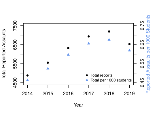
The total number of assaults reported across schools increased steadily from 2014 to 2018, growing by nearly 50% before falling in 2019 (see Figure 2). The total in-person student population was relatively stable over this time period, remaining close to 10.6 million.
Campus crime numbers in this dataset are a direct tally of the individual assaults for which a student voluntarily made a formal report to campus authorities. Note that those reports do not arise from a survey process or broad inquiry about student experiences; on its own, this dataset contains no information about underreporting. For complementary information about reporting rates, we consider the National Crime Victimization Survey (NCVS). The NCVS is a large-scale annual survey conducted on behalf of the behalf of the US Bureau of Justice Statistics to determine incidence rates of personal and property crimes, including sexual assault. This survey dates back 50 years, and one of its primary objectives is to quantify the extent of crime not reported to authorities. By attempting to measure crimes not reported to authorities, the NCVS provides additional context which is absent from the college campus Clery Report data.
4 Methodology
For a particular school in a particular year , suppose that the true, unknown number of assaults comes from a Poisson distribution with rate parameter . Further suppose that each of those assaults is independently reported, or not reported, with probability of reporting equal to . This produces the reported value that we observe, according to a binomial thinning process:
| (1) |
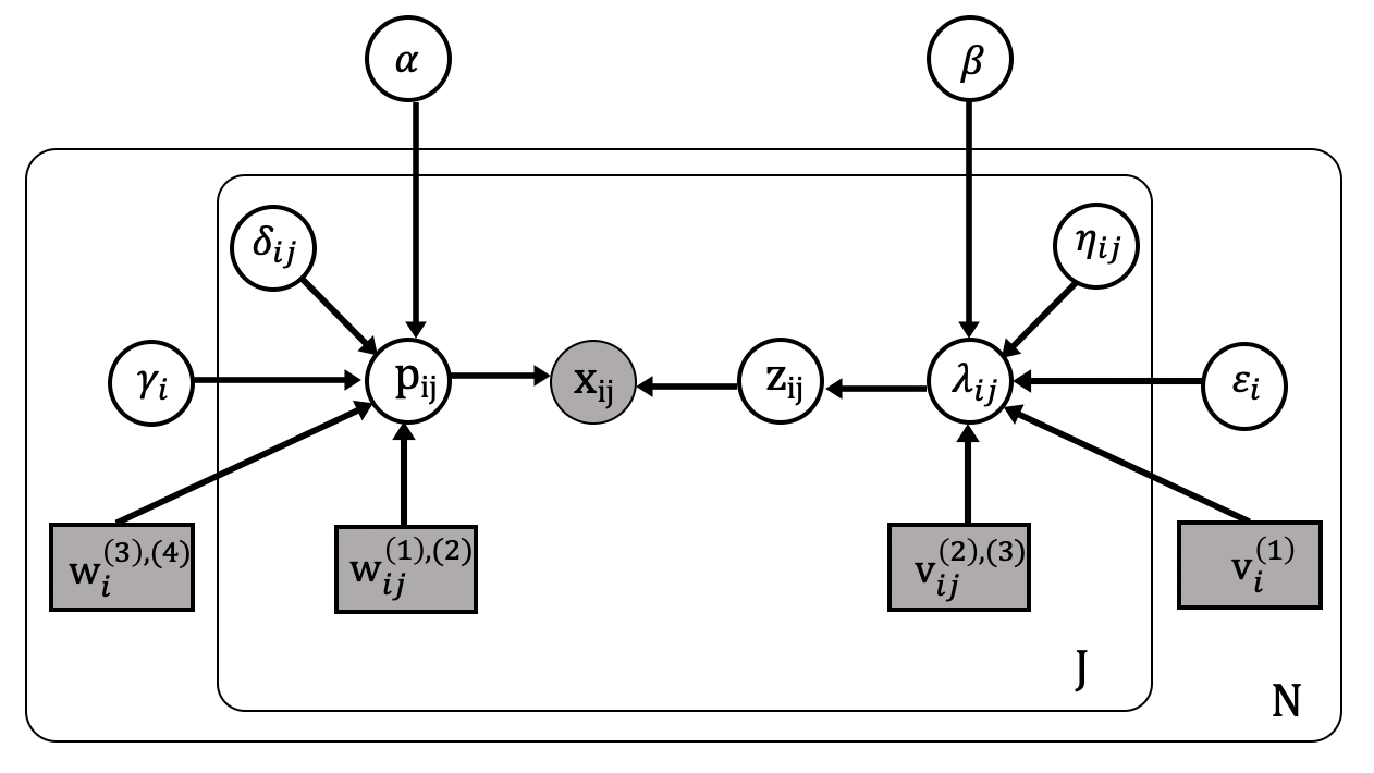
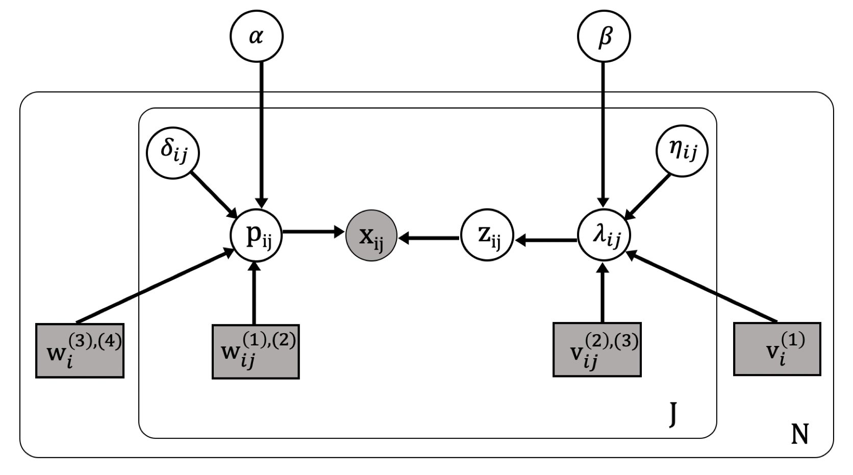
With this likelihood model, we construct a hierarchical generative model for the reported campus sexual assault data. The proposed hierarchical model, diagrammed in Figure 3, entails a component describing the reporting probability, and a component describing the Poisson rate governing the true number of assaults. A common approach in the underreporting literature is to model and/or as deterministically equal to a linear function of covariates (Dvorzak and Wagner, 2016; Stoner, Economou and Drummond Marques da Silva, 2019; de Oliveira et al., 2021). To provide additional flexibility, we instead model the Poisson rate and reporting probability as random functions of their respective covariates. Full details of each model component are discussed below.
4.1 Modeling z
For each record in the dataset, we suppose the true number of assaults arises from a Poisson distribution parameterized by , where depends on observed characteristics v of school in year as follows:
| (2) | |||||
| (3) | |||||
The covariates associated with are:
| : | degree of urbanization of school ’s campus |
|---|---|
| 1 = urban | |
| 2 = suburban | |
| 3 = rural | |
| : | log(number of in-person students) for school in year |
| : | (fraction of women in student body at school in year - 0.5)2 |
This generative model considers in-person student population, degree of campus urbanization, and student body gender composition333The gender categories reported by NCES are currently ”male” and ”female”. as covariates of interest. The functional form of equations (2) - (3) implies that for the expected number of assaults we have:
| (4) | |||||
This modeling choice allows for the possibility that the number of assaults does not scale linearly with the number of in-person students. Because the number of interpersonal interactions does not always scale linearly with community size, this type of ”power law” dynamic has been observed for various social phenomena, including crime (Bettencourt et al., 2007; Chang et al., 2018).
Incorporating separate intercepts in (3) allows for different incidence patterns at urban, suburban, and rural schools. This decision is motivated by the national differences in violent crime victimization rates across locales of varying urbanization (Truman and Langton, 2014, 2015; Truman and Morgan, 2016; Morgan and Kena, 2018; Morgan and Truman, 2018; Morgan and Thompson, 2020).
Gender composition of the student body is included as a covariate because most perpetrators of sexual assault are men, while most victims are women (Sinozich and Langton, 2014). We center the proportion of women in the student body by subtracting 0.5, and square this value, to allow for the possibility that schools with more extreme gender imbalances may have different rates of assault.
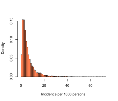
Per-school intercepts allow for between-school differences in assault incidence patterns which are not otherwise captured by covariates. Per-record noise terms allow for within-school differences across years. Supposing that (linear relationship between student population and number of assaults) and (no relationship between student body gender composition and expected number of assaults), priors on , , and intercepts are set so that the resulting distribution over assaults per 1000 persons roughly corresponds with external estimates from the National Crime Victimization Survey (NCVS). The resulting distribution is displayed in Figure 5. Note that, conditional on covariates, the Poisson rate follows a lognormal distribution, leading to a number of assaults whose marginal distribution is overdispersed relative to a Poisson.
| 18-20 | 21-24 | 12+ | |
|---|---|---|---|
| 2014 | 1.2* | 3.8 | 1.1 |
| 2015 | 3.2 | 1.6* | 1.6 |
| 2016 | 3.8 | 1.8 | 1.1 |
| 2017 | 8.6 | 2.4 | 1.4 |
| 2018 | 10.1 | 6.0 | 2.7 |
| 2019 | 7.1 | 6.4 | 1.7 |
The NCVS is a large sample survey conducted annually on behalf of the US Bureau of Justice Statistics to determine incidence rates of personal and property crimes. This survey includes crimes reported and not reported the police. Over the 2014-2019 time period, the estimated incidence of sexual assault in the overall population aged 12 and older ranged from 1.1 to 2.7 per 1000 persons. As shown in Table 5, estimated incidence skewed higher in the 18-20 and 21-24 age groups, which are particularly relevant to the college student population.
4.2 Modeling p
As formulated in Equation 1, the reported number of assaults arises from the latent true number of assaults and the reporting probability . Having discussed a model for , we now turn to modeling the reporting probability . Of the total assaults occurring at school in year , suppose that each individual assault is reported, independently, with probability , where depends on observed characteristics w of school in year as follows:
| (5) | |||||
The covariates associated with are:
| : | school issues associate degrees only () |
|---|---|
| : | school substantially engaged in religious instruction () |
| : | (women as fraction of student body at school in year - 0.5) |
| : | Pell grant recipients as fraction of student body at school in year , median centered |
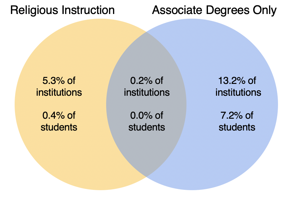
The reporting probability at school in year accounts for two school-level covariates that are fixed across years, and two that vary. The first fixed school-level covariate is , an indicator for whether school is a junior college, issuing only associate degrees as opposed to bachelor degrees or higher. The reporting probability also incorporates an indicator for whether school is substantially engaged in religious instruction. A theological seminary, for instance, would satisfy this definition, whereas a religiously affiliated liberal arts college would not. The inclusion of these school-level random effects encourages the probabilities for an individual school to exhibit similarity across years. Junior colleges comprise roughly 13% of institutions in the dataset, and account for 7% of total in-person students. Institutions of religious instruction make up a relatively smaller portion of the dataset, and generally have small student populations. These two categories of institution have negligible overlap, as detailed in Figure 6.
Gender composition of a school’s student body also contributes to the reporting probability, and varies across years. Many institutions in this dataset have approximately gender-balanced student populations. Across records, the proportion of female students is centered around 57%, with smaller peaks at each end of the spectrum corresponding to all-male and all-female schools. The final covariate incorporated in the reporting rate is the fraction of Pell grant recipients in the student body. Pell grants are federal financial aid awarded to students on the basis of exceptional financial need. This variable is included as a proxy for socioeconomic status, which research indicates may be correlated with reporting rates (Fisher et al., 2003; Sabina and Ho, 2014). The median percentage of undergraduates receiving Pell grants is 36%, and values are more widely spread over the unit interval compared to the gender composition composition covariate.
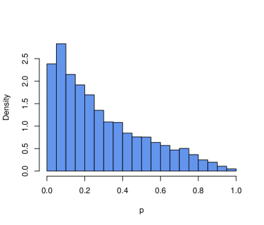
As in the model of Poisson rate , per-school intercepts in Equation 5 allow for between-school differences in assault incidence patterns not captured by covariates, while per-record noise terms allow for within-school differences across years. Supposing that , priors on , , and intercepts are chosen to be broadly consistent with NCVS estimates of the percentage of sexual assaults reported to police. Over the 2014-2019 time period, the estimated rate of reporting to police ranged from 23% to 40% in the overall 12+ population, while reporting rates for the 18-20 and 21-24 age groups tended to be lower (see Table 8). The induced prior distribution over values of , when , is depicted in Figure 8 below.
| 18-20 | 21-24 | 12+ | |
|---|---|---|---|
| 2014 | 0.0* | 16.48 | 33.6 |
| 2015 | 10.6* | 26.0* | 32.5 |
| 2016 | 10.2* | 31.0* | 23.2 |
| 2017 | 45.3 | 38.3* | 40.4 |
| 2018 | 11.0* | 10.2* | 24.9 |
| 2019 | 17.5* | 24.7* | 33.9 |
In these models of and , global coefficients and encourage the sharing of information across schools, while school-level terms and capture local properties of individual schools. This partial pooling model structure is a compromise between complete pooling, in which no school-level differences are permitted ( and omitted), and no pooling, in which each school is modeled separately from all others, with its own coefficient vectors and . Compared to the complete-pooling and no-pooling alternatives, the partial pooling model assigns higher likelihood to held-out observational data- refer to Appendix C for details.
4.3 Inference
The model does not admit closed form expressions for posterior quantities of interest. We draw samples from the joint posterior distribution over latent variables via MCMC. The true number of assaults is a discrete latent variable, which presents an obstacle to gradient-based sampling schemes such as Hamiltonian Monte Carlo (HMC). However, this can be circumvented by marginalizing out . Instead of working with , one can take advantage of the fact that conditional on the event rate and reporting probability , but not the true number of assaults , the reported number of assaults follows a Poisson distribution:
See Appendix B for derivation. This marginalizes out the discrete latent variable , allowing for gradient-based MCMC sampling from the posterior . However, the latent true number of assaults is also a quantity of interest. To address this, first note the conditional distribution of the number of unreported assaults, (where ):
Because is conditionally independent of the covariates and given latent parameters and , it is equivalently true that
Each MCMC sample drawn from (approximately) can be augmented by sampling a corresponding from . The sampled value can then be added to the observed count to produce a sample for the latent count . Altogether, the sample constitutes an MCMC sample from . This sampling procedure is outlined in Algorithm 1, and can be conveniently implemented in a probabilistic programming language. Posterior inference for this work was conducted using HMC in Stan (Stan Development Team, 2023).
-
•
Data
-
•
Covariates
-
•
Index set (pairs (i,j) for which the dataset contains a record
-
•
MCMC algorithm SAMPLER (e.g. HMC)
-
•
Markov chain length
4.4 Model Assessment
Fully-observed data including the true total number of assaults is not available, and thus cannot be used for model validation. Instead, the predictive distribution provides information about the quality of the model fit. The posterior distribution of the latent variables implies a predictive distribution over future observations and, accordingly, over summary statistics of future observations. This motivates the notion of posterior predictive checks (Guttman, 1967; Box, 1980; Rubin, 1984; Gelman, Meng and Stern, 1996): that a satisfactory model will yield predictive distributions over key summary statistics under which the actual values observed in the dataset are not extreme. As detailed in Moran, Blei and Ranganath (2019) and Li and Huggins (2022), such posterior predictive checks can be overly optimistic about model fit due to double use of the data (both to fit the model and to evaluate it). The aforementioned works propose randomly reserving a portion of the original dataset to use exclusively for model assessment, an approach that demonstrably achieves a more accurate gauge of model performance by avoiding the pitfall of data reuse. In the spirit of this suggestion, roughly 20% of entries in the campus sexual assault dataset are held out, with the remaining 80% used for posterior inference. Held out data points are sampled at the level of (school, year) pairs. The held out data set includes records from all years in scope (2014-2019), and does not contain data from any additional schools not seen in the main sample. Predictive samples for the held out data points are generated as follows.
-
•
Index set (pairs (i,j) for which the held out dataset contains a record )
-
•
Covariates for held out dataset
-
•
Posterior distribution
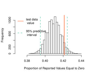
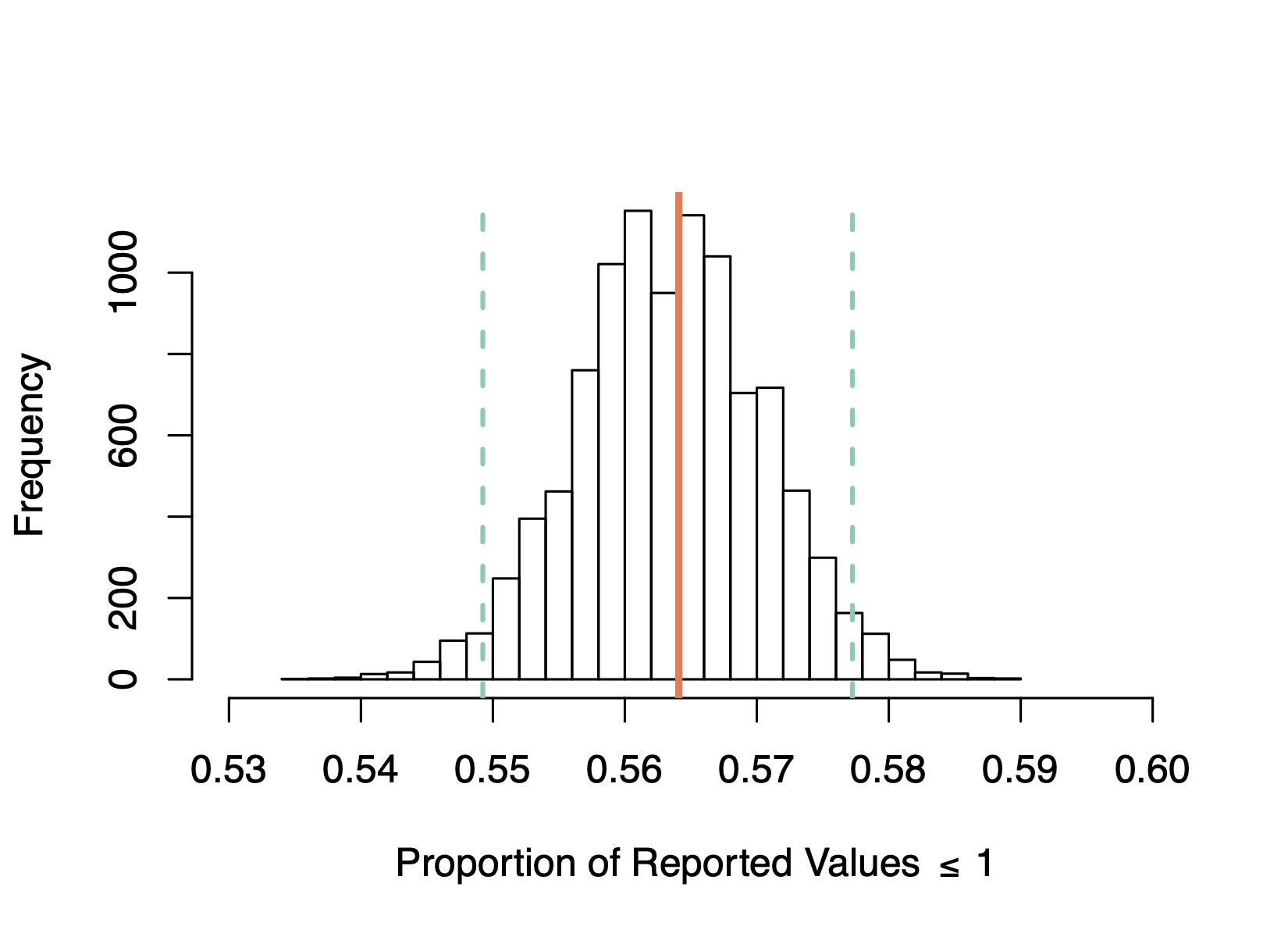
As noted in Section 3, each year many schools had zero reported assaults, and the median number of reports was 1. Generating 10,000 resampled datasets according to Algorithm 2 and calculating the proportion of records with zero reported assaults produces the distribution shown below in Figure 9(a). Within the held out dataset 42.1% of records had zero reported assaults, while values ranged from roughly 38% to 44% in datasets sampled from the predictive distribution. The distribution of reported assault numbers has been pulled slightly away from the extreme end, such that the observed proportion of zeroes falls toward the high end of the predictive distribution. However, the median number of assaults was equal to 1 in all datasets sampled from the predictive distribution, and the true proportion of held-out records with assaults sits comfortably within its respective predictive distribution (Figure 9(b)). Overall, the model adequately captures the bottom-heaviness of the distribution of reported assault numbers.
 |
 |
| (a) | (b) |
 |
 |
| (c) | (d) |
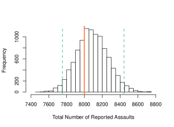
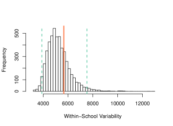
Other quantities of interest are the total number of reported assaults and the amount of within-school variability. The predicted number of assaults reported by an individual school should not be too rigid or too flexible over time, relative to the trends seen in the actual data. This summary statistic is quantified as . The total number of reported assaults and the within-school variability observed in the held out dataset are both plausible under their respective predictive distributions, shown in Figure 9(c)-(d), suggesting that the model adequately captures these characteristics of the data.
4.5 Capabilities and Limitations
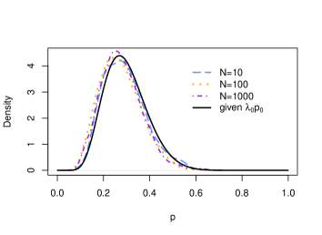
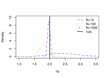
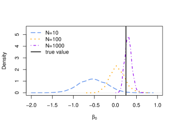
Let us pause to examine what this estimation method can and cannot do in terms of resolving the central identifiability issue introduced in Sections 1 and 2. First, consider a toy example in which are latent and are observed. The observed dataset identifies the product , while only the prior distributions provide information about and individually. The posterior distribution of the product concentrates as the number of observations increases. The posterior distributions of and , however, do not become arbitrarily concentrated in the infinite data limit, but rather approach and respectively, as demonstrated in Figure 10.
Furthermore, the posterior distribution will not necessarily be centered at the true value (and likewise for ); the data provide information about the product , but conditional on , posterior estimates of and are determined by their respective prior distributions.
 |
 |
| (a) | (b) |
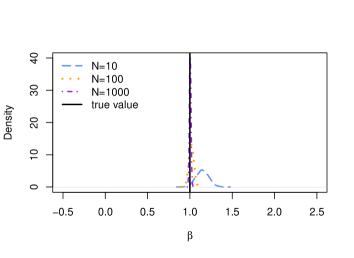
A similar relationship emerges when the toy model is extended to include covariates for and . Let and for . For latent counts are generated as , and we observe the reported counts . Performing posterior inference on data simulated from this model reveals that increasing the amount of observational data is more effective at reducing posterior uncertainty about the slope parameters and than about the intercepts and . Figure 11 illustrates the relative difficulty of learning one of the intercept parameters from data.
 |
 |
| (a) | (b) |
In light of these dynamics, Appendix E explores sensitivity to the prior information elicited from NCVS estimates. While some reasons for not reporting a sexual assault are less relevant in a survey setting (such as fear of retaliation or lack of faith that the perpetrator will be held accountable), it is nevertheless plausible that some NCVS respondents choose not to disclose their sexual assault victimization. In line with the discussion in this section, inferences about the role of covariates are relatively more stable if the extent of underreporting is larger than estimated by NCVS, while inferences about the true overall incidence and reporting rate exhibit more sensitivity.
5 Results
5.1 Role of Covariates
Sampling from the model in Section 4 yields the posterior means and quartiles given in Table 1 below.
| Variable | Mean | 25% | Median | 75% | R hat† |
|---|---|---|---|---|---|
| 0.82 | 0.81 | 0.82 | 0.84 | 1.00 | |
| -4.05 | -4.53 | -4.05 | -3.56 | 1.00 | |
| -4.54 | -4.67 | -4.54 | -4.42 | 1.00 | |
| -4.40 | -4.53 | -4.40 | -4.28 | 1.00 | |
| -4.32 | -4.45 | -4.32 | -4.21 | 1.00 | |
| -1.43 | -1.50 | -1.43 | -1.36 | 1.00 | |
| -1.97 | -2.06 | -1.97 | -1.88 | 1.00 | |
| -2.48 | -2.73 | -2.48 | -2.23 | 1.00 | |
| 0.49 | 0.26 | 0.49 | 0.73 | 1.00 | |
| -3.00 | -3.18 | -3.00 | -2.83 | 1.00 |
| †R hat, also known as the potential scale reduction factor, is a convergence diagnostic |
| proposed in Gelman and Rubin (1992) |
The posterior distribution for is concentrated around 0.82, which corresponds to sub-linear growth in the expected number of assaults as a function of number of students. The proposed the power law relationship between student population and expected number of assaults (4) implies a similar relationship between student population and the expected per-capita rate of assaults, :
Consequently, the posterior distribution suggests an inverse relationship between the size of the student population and the expected per-capita number of assaults in a given year. With all other covariates held equal, we expect a school to have 13% more assaults per capita than an equivalent school twice its size, and 28% more than a school 4 times its size. Similarly, because the posterior distribution suggests , the variance of the per capita number of assaults, , scales inversely with the number of students. With other covariates held constant, the expected number of assaults per capita is more variable at small schools than at large ones.
Posterior distributions for the intercepts , , and are similar to each other. Results are mildly suggestive of higher sexual assault incidence in rural areas than in cities, but do not reveal a substantial difference in expected number of assaults based on degree of campus urbanization. The negative values for suggest that a gender imbalance in a school’s student body is associated with lower expected incidence of sexual assault, while suggests that a higher proportion of female students corresponds to a higher reporting probability. Conversely, a higher proportion of students receiving Pell grants (a proxy for lower socioeconomic status) appears associated with a lower probability of reporting. Negative estimates for and signal lower expected reporting probabilities for junior colleges and institutions of religious instruction.
5.2 Systemwide Results
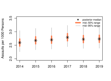
Drawing posterior samples of the true number of assaults at each school induces a distribution over the total number of assaults across schools each year. The posterior median for total assaults ranges from 2.6 to 2.8 per 1000 persons over the 2014-2019 time period. Although the median estimated incidence is higher in later years compared to 2014, posterior uncertainty is large enough that the true trend in incidence could conceivably be flat or even increasing, as can be seen in Figure 12 below.
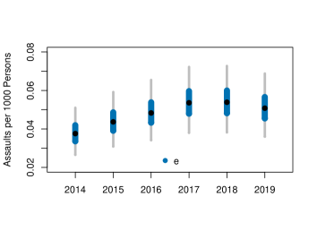
Posterior estimates of the true reporting rate, however, show more movement over time. Figure 13 depicts posterior summaries for the actual number of reported assaults across schools as a fraction of the estimated true number of assaults. The posterior median reporting rate was lowest in 2014, at 17.3%, and highest in 2018 at 24.2%, with reporting rates trending upward over those years.
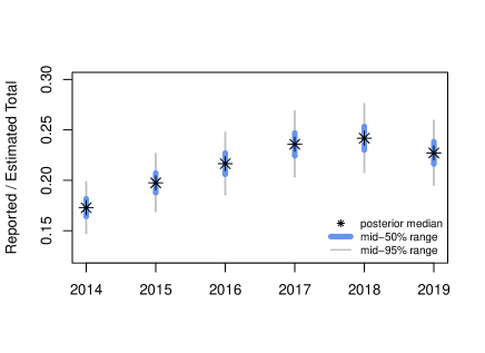
Taken together, these two results suggest that the increase in total sexual assaults reported nationwide over the 2014-2019 period is more likely attributable to an increase in reporting rates than an increase in the true number of assaults that occurred.
5.3 School-Level Results
While the systemwide increase in reported assaults may be more easily explained by an increase in reporting rates, aggregate trends are not necessarily representative of the dynamics at an individual school. Examining the posterior medians of the reporting rate and true incidence per 1000 persons across all records in the dataset reveals considerable heterogeneity, as displayed in Figure 14.
 |
 |
| (a) | (b) |
While sexual assault is susceptible to underreporting at all schools, the estimated degree of underreporting varies widely. Figure 14(b) illustrates that some schools have extremely low reporting probabilities, while others are considerably higher than the population-level reporting rates published in the NCVS. This variation across schools has implications for how individual schools should interpret their reported crime statistics. With only the prior belief that sexual assault is significantly underreported, one might be equally inclined to attribute an increase in reported assaults at any school to an increase in the reporting probabilities. However, this may lead to flawed conclusions.
Suppose that for a particular school, the true number of assaults in a future year, included in the dataset, remains the same as the true number of assaults in 2019. With an unchanged number of true assaults, how large of a change in the reported number of assaults is plausible due to variation in the reporting probability alone? For school , the predictive distribution for a future year’s number of reported assaults can be sampled as follows.
-
(1)
Draw from model’s posterior distribution
-
(2)
Draw
-
(3)
Set
-
(4)
Draw
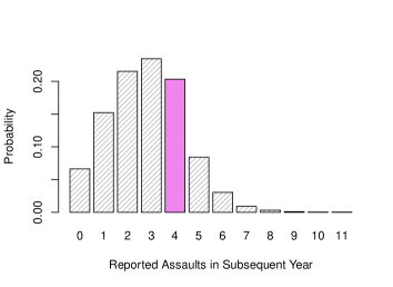
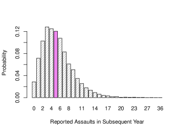
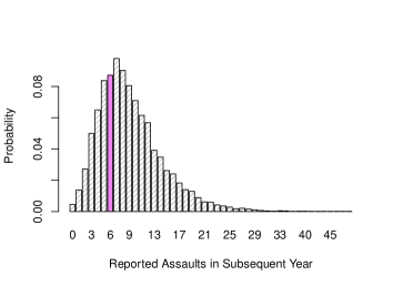
Randolph College and the University of South Carolina-Columbia (USCC) had a similar number of reported assaults in 2019 (4 and 5 respectively). However, Randolph College’s estimated reporting rate was considerably higher, with a posterior median of 53% compared to only 14% at USCC. Assuming that the true number of assaults is held constant, the predictive distributions for the number of reported assaults are shown in Figure 15.
 |
 |
| (a) | (b) |
Under this scenario, there is a roughly 13% chance of an increased number of reported assaults at Randolph College in a subsequent year due to variation in the reporting rate, and less than a 1% chance of the reported number to double to 8 or more. At USCC, variation in reporting rate has a comparatively larger chance of producing an increased number of reported assaults (42%), and a 12% chance of doubling the number of reported assaults to 10 or more.
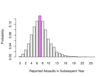
Ursinus College and Temple University provide another illustration of such school-level differences. Of the two, Ursinus had a much higher estimated reporting probability in 2019, and changes in reporting probability are comparatively less likely to drive an increase in reported assaults at Ursinus compared to Temple, as can be seen from their respective predictive distributions in Figure 16.
 |
 |
| (a) | (b) |
These disparities underscore the opaque nature of reported campus sexual assault data and the potential pitfalls of a one-size-fits-all approach to interpreting school-level reports over time.
6 Discussion
Colleges and universities prioritize reducing the incidence of sexual assault on their campuses, but underreporting diminishes the interpretability of their published sexual assault incidence data. This paper constructs a generative model of underreported campus sexual assault data which allows for estimation of true incidence and reporting rates. Fitting this model reveals that lower socioeconomic status, as measured by the percentage of a school’s undergraduates receiving Pell grants, appears associated with a lower probability of reporting. Status as a junior college or institution of religious instruction appear similarly associated with lower reporting probability, while gender imbalance in a school’s student body is associated with lower true incidence of assault.
For the overall college population, estimated incidence of sexual assault remained fairly stable over 2014-2019, while reporting probabilities increased. Results at individual schools, however, varied widely. Estimates of school-level incidence and reporting probabilities may help university officials, for instance Title IX coordinators, assess the effectiveness of initiatives to reduce incidence of sexual assault or to familiarize students with reporting resources, and decide where to make changes and improvements moving forward.
One avenue for future work concerns repeat victimizations of the same individual. High-frequency series victimizations, for instance in the case of patterns of intimate partner violence, can produce extreme values in the reported number of assaults. As an example, in 2017 the University of Nebraska-Lincoln received 104 reports of sexual assault corresponding to the same victim and perpetrator. Such extreme outliers are not easily accommodated, and in particular may violate the modeling assumption that the reporting decisions for each assault are independent (conditional on reporting probability). Violations of the independence assumption can degrade the quality of posterior inferences- see Appendix D for further details. More broadly, the Bureau of Justice Statistics has acknowledged the difficulty of accurately incorporating series victimization in its national crime estimates (Lauritsen et al., 2012).
[Acknowledgments]
The authors would like to thank the referees, Associate Editor and the Editor for their constructive comments and suggestions that improved the quality of this paper.
David M. Blei is also affiliated with the Department of Computer Science at Columbia University.
The second author is supported by NSF IIS-2127869, NSF DMS-2311108, ONR N000142412243, and the Simons Foundation.
Appendices \sdescriptionThis file contains Appendices A-E to the main text. {supplement} \stitleCode and Data \sdescriptionThis file contains R and Stan implementations of methods from the main text, along with preprocessed data.
References
- Axelson (2019) {barticle}[author] \bauthor\bsnmAxelson, \bfnmBen\binitsB. (\byear2019). \btitleThese are the 45 Upstate NY college campuses that reported the most rapes, ranked. \bjournalNewYorkUpstate.com. \bnote14 May 2019, https://www.newyorkupstate.com/news/g66l-2019/05/b1452bae03654/these-are-the-45-ny-college-campuses-that-reported-the-most-rapes-ranked.html. Accessed: 3 Aug 2023. \endbibitem
- Bailey et al. (2005) {barticle}[author] \bauthor\bsnmBailey, \bfnmT C\binitsT. C., \bauthor\bsnmCarvalho, \bfnmM S\binitsM. S., \bauthor\bsnmLapa, \bfnmT M\binitsT. M., \bauthor\bsnmSouza, \bfnmW V\binitsW. V. and \bauthor\bsnmBrewer, \bfnmM J\binitsM. J. (\byear2005). \btitleModeling of under-detection of cases in disease surveillance. \bjournalAnnals of Epidemiology \bvolume15 \bpages335–343. \endbibitem
- Bettencourt et al. (2007) {barticle}[author] \bauthor\bsnmBettencourt, \bfnmLuís M A\binitsL. M. A., \bauthor\bsnmLobo, \bfnmJosé\binitsJ., \bauthor\bsnmHelbing, \bfnmDirk\binitsD., \bauthor\bsnmKühnert, \bfnmChristian\binitsC. and \bauthor\bsnmWest, \bfnmGeoffrey B\binitsG. B. (\byear2007). \btitleGrowth, innovation, scaling, and the pace of life in cities. \bjournalProceedings of the National Academy of Sciences \bvolume104 \bpages7301–7306. \endbibitem
- Box (1980) {barticle}[author] \bauthor\bsnmBox, \bfnmGeorge EP\binitsG. E. (\byear1980). \btitleSampling and Bayes’ inference in scientific modelling and robustness. \bjournalJournal of the Royal Statistical Society Series A: Statistics in Society \bvolume143 \bpages383–404. \endbibitem
- Bracher and Held (2021) {barticle}[author] \bauthor\bsnmBracher, \bfnmJohannes\binitsJ. and \bauthor\bsnmHeld, \bfnmLeonhard\binitsL. (\byear2021). \btitleA marginal moment matching approach for fitting endemic-epidemic models to underreported disease surveillance counts. \bjournalBiometrics \bvolume77 \bpages1202–1214. \endbibitem
- Cantor et al. (2021) {barticle}[author] \bauthor\bsnmCantor, \bfnmDavid\binitsD., \bauthor\bsnmSteiger, \bfnmDarby M.\binitsD. M., \bauthor\bsnmTownsend, \bfnmReanne\binitsR., \bauthor\bsnmHartge, \bfnmJohn Y.\binitsJ. Y., \bauthor\bsnmFay, \bfnmRobert E.\binitsR. E., \bauthor\bsnmWarren, \bfnmAntonia\binitsA., \bauthor\bsnmHeaton, \bfnmLeanne L.\binitsL. L., \bauthor\bsnmKaasa, \bfnmSuzanne\binitsS., \bauthor\bsnmMaitland, \bfnmAaron\binitsA., \bauthor\bsnmSun, \bfnmHanyu\binitsH., \bauthor\bsnmNorman, \bfnmGreg\binitsG., \bauthor\bsnmJones, \bfnmMichael\binitsM., \bauthor\bsnmCatalano, \bfnmShannan\binitsS. and \bauthor\bsnmBeck, \bfnmAllen J.\binitsA. J. (\byear2021). \btitleMethodological research to support the National Crime Victimization Survey: Self-report data on rape and sexual assault–Pilot test. \bjournalBureau of Justice Statistics \bvolumeNCJ 256011. \endbibitem
- Chang et al. (2018) {barticle}[author] \bauthor\bsnmChang, \bfnmYuSang\binitsY., \bauthor\bsnmChoi, \bfnmSungSup Brian\binitsS. B., \bauthor\bsnmLee, \bfnmJinsoo\binitsJ. and \bauthor\bsnmJin, \bfnmWon Chang\binitsW. C. (\byear2018). \btitlePopulation Size vs. Number of Crimes: Is the Relationship Superlinear? \bjournalInternational Journal of Information Systems and Social Change (IJISSC) \bvolume9 \bpages26–39. \endbibitem
- Cuellar (2018) {barticle}[author] \bauthor\bsnmCuellar, \bfnmMaria\binitsM. (\byear2018). \btitleTrends in self-reporting of marijuana consumption in the United States. \bjournalStatistics and Public Policy \bvolume5 \bpages1–10. \endbibitem
- de Oliveira, Loschi and Assunção (2017) {barticle}[author] \bauthor\bparticlede \bsnmOliveira, \bfnmGuilherme Lopes\binitsG. L., \bauthor\bsnmLoschi, \bfnmRosangela Helena\binitsR. H. and \bauthor\bsnmAssunção, \bfnmRenato Martins\binitsR. M. (\byear2017). \btitleA random-censoring Poisson model for underreported data. \bjournalStatistics in medicine \bvolume36 \bpages4873–4892. \endbibitem
- de Oliveira et al. (2021) {barticle}[author] \bauthor\bparticlede \bsnmOliveira, \bfnmGuilherme L\binitsG. L., \bauthor\bsnmOliveira, \bfnmJuliane F\binitsJ. F., \bauthor\bsnmPescarini, \bfnmJúlia M\binitsJ. M., \bauthor\bsnmAndrade, \bfnmRoberto F S\binitsR. F. S., \bauthor\bsnmNery, \bfnmJoilda S\binitsJ. S., \bauthor\bsnmIchihara, \bfnmMaria Y\binitsM. Y., \bauthor\bsnmSmeeth, \bfnmLiam\binitsL., \bauthor\bsnmBrickley, \bfnmElizabeth B\binitsE. B., \bauthor\bsnmBarreto, \bfnmMaurício L\binitsM. L., \bauthor\bsnmPenna, \bfnmGerson O\binitsG. O. \betalet al. (\byear2021). \btitleEstimating underreporting of leprosy in Brazil using a Bayesian approach. \bjournalPLoS Neglected Tropical Diseases \bvolume15. \endbibitem
- Dvorzak and Wagner (2016) {barticle}[author] \bauthor\bsnmDvorzak, \bfnmMichaela\binitsM. and \bauthor\bsnmWagner, \bfnmHelga\binitsH. (\byear2016). \btitleSparse Bayesian modelling of underreported count data. \bjournalStatistical Modelling \bvolume16 \bpages24–46. \endbibitem
- Fader and Hardie (2000) {barticle}[author] \bauthor\bsnmFader, \bfnmPeter S\binitsP. S. and \bauthor\bsnmHardie, \bfnmBruce GS\binitsB. G. (\byear2000). \btitleA note on modelling underreported Poisson counts. \bjournalJournal of Applied Statistics \bvolume27 \bpages953–964. \endbibitem
- Fernández-Fontelo et al. (2019) {barticle}[author] \bauthor\bsnmFernández-Fontelo, \bfnmAmanda\binitsA., \bauthor\bsnmCabaña, \bfnmAlejandra\binitsA., \bauthor\bsnmJoe, \bfnmHarry\binitsH., \bauthor\bsnmPuig, \bfnmPedro\binitsP. and \bauthor\bsnmMoriña, \bfnmDavid\binitsD. (\byear2019). \btitleUntangling serially dependent underreported count data for gender-based violence. \bjournalStatistics in Medicine \bvolume38 \bpages4404–4422. \endbibitem
- Fisher et al. (2003) {barticle}[author] \bauthor\bsnmFisher, \bfnmBonnie S\binitsB. S., \bauthor\bsnmDaigle, \bfnmLeah E\binitsL. E., \bauthor\bsnmCullen, \bfnmFrancis T\binitsF. T. and \bauthor\bsnmTurner, \bfnmMichael G\binitsM. G. (\byear2003). \btitleReporting sexual victimization to the police and others: Results from a national-level study of college women. \bjournalCriminal Justice and Behavior \bvolume30 \bpages6–38. \endbibitem
- Gelman, Meng and Stern (1996) {barticle}[author] \bauthor\bsnmGelman, \bfnmAndrew\binitsA., \bauthor\bsnmMeng, \bfnmXiao-Li\binitsX.-L. and \bauthor\bsnmStern, \bfnmHal\binitsH. (\byear1996). \btitlePosterior predictive assessment of model fitness via realized discrepancies. \bjournalStatistica sinica \bpages733–760. \endbibitem
- Gelman and Rubin (1992) {barticle}[author] \bauthor\bsnmGelman, \bfnmAndrew\binitsA. and \bauthor\bsnmRubin, \bfnmDonald B\binitsD. B. (\byear1992). \btitleInference from iterative simulation using multiple sequences. \bjournalStatistical Science \bpages457–472. \endbibitem
- Goodman (2017) {barticle}[author] \bauthor\bsnmGoodman, \bfnmJames\binitsJ. (\byear2017). \btitleState steps up efforts to make colleges more responsive to sexual assault allegations. \bjournalDemocrat and Chronicle. \bnote10 July 2017, https://www.democratandchronicle.com/story/news/2017/07/10/training-session-sexual-assault-puts-priority-understanding-trauma/454590001/. Accessed: 3 Aug 2023. \endbibitem
- Guttman (1967) {barticle}[author] \bauthor\bsnmGuttman, \bfnmIrwin\binitsI. (\byear1967). \btitleThe use of the concept of a future observation in goodness-of-fit problems. \bjournalJournal of the Royal Statistical Society: Series B (Methodological) \bvolume29 \bpages83–100. \endbibitem
- Jaynes (1968) {barticle}[author] \bauthor\bsnmJaynes, \bfnmEdwin T\binitsE. T. (\byear1968). \btitlePrior probabilities. \bjournalIEEE Transactions on Systems Science and Cybernetics \bvolume4 \bpages227–241. \endbibitem
- Jeffreys (1946) {barticle}[author] \bauthor\bsnmJeffreys, \bfnmHarold\binitsH. (\byear1946). \btitleAn invariant form for the prior probability in estimation problems. \bjournalProceedings of the Royal Society of London. Series A. Mathematical and Physical Sciences \bvolume186 \bpages453–461. \endbibitem
- Kruttschnitt, Kalsbeek and House (2014) {bbook}[author] \beditor\bsnmKruttschnitt, \bfnmCandace\binitsC., \beditor\bsnmKalsbeek, \bfnmWilliam D.\binitsW. D. and \beditor\bsnmHouse, \bfnmCarol C.\binitsC. C., eds. (\byear2014). \btitleEstimating the incidence of rape and sexual assault. \bpublisherWashington, DC: The National Academies Press. \endbibitem
- Kumara and Chin (2005) {barticle}[author] \bauthor\bsnmKumara, \bfnmSSP\binitsS. and \bauthor\bsnmChin, \bfnmHoong Chor\binitsH. C. (\byear2005). \btitleApplication of Poisson underreporting model to examine crash frequencies at signalized three-legged intersections. \bjournalTransportation Research Record \bvolume1908 \bpages46–50. \endbibitem
- Lauritsen et al. (2012) {barticle}[author] \bauthor\bsnmLauritsen, \bfnmJanet L.\binitsJ. L., \bauthor\bsnmGatewood Owens, \bfnmJennifer\binitsJ., \bauthor\bsnmPlanty, \bfnmMichael\binitsM., \bauthor\bsnmRand, \bfnmMichael R.\binitsM. R. and \bauthor\bsnmTruman, \bfnmJennifer L.\binitsJ. L. (\byear2012). \btitleMethods for Counting High-Frequency Repeat Victimizations in the National Crime Victimization Survey. \bjournalBureau of Justice Statistics \bvolumeNCJ 237308. \endbibitem
- Letouzey, Denis and Gilleron (2000) {binproceedings}[author] \bauthor\bsnmLetouzey, \bfnmFabien\binitsF., \bauthor\bsnmDenis, \bfnmFrançois\binitsF. and \bauthor\bsnmGilleron, \bfnmRémi\binitsR. (\byear2000). \btitleLearning from positive and unlabeled examples. In \bbooktitleInternational Conference on Algorithmic Learning Theory \bpages71–85. \bpublisherSpringer. \endbibitem
- Li and Huggins (2022) {barticle}[author] \bauthor\bsnmLi, \bfnmJiawei\binitsJ. and \bauthor\bsnmHuggins, \bfnmJonathan H\binitsJ. H. (\byear2022). \btitleCalibrated Model Criticism Using Split Predictive Checks. \bjournalarXiv preprint arXiv:2203.15897. \endbibitem
- Ma and Li (2010) {bincollection}[author] \bauthor\bsnmMa, \bfnmJianming\binitsJ. and \bauthor\bsnmLi, \bfnmZheng\binitsZ. (\byear2010). \btitleBayesian modeling of frequency-severity indeterminacy with an application to traffic crashes on two-lane highways. In \bbooktitleICCTP 2010: Integrated Transportation Systems: Green, Intelligent, Reliable \bpages1022–1033. \endbibitem
- Moran, Blei and Ranganath (2019) {barticle}[author] \bauthor\bsnmMoran, \bfnmGemma E.\binitsG. E., \bauthor\bsnmBlei, \bfnmDavid M.\binitsD. M. and \bauthor\bsnmRanganath, \bfnmRajesh\binitsR. (\byear2019). \btitlePopulation predictive checks. \bjournalarXiv preprint arXiv:1908.00882. \endbibitem
- Moreno and Giron (1998) {barticle}[author] \bauthor\bsnmMoreno, \bfnmElias\binitsE. and \bauthor\bsnmGiron, \bfnmJavier\binitsJ. (\byear1998). \btitleEstimating with incomplete count data A Bayesian approach. \bjournalJournal of Statistical Planning and Inference \bvolume66 \bpages147–159. \endbibitem
- Morgan and Kena (2018) {barticle}[author] \bauthor\bsnmMorgan, \bfnmRachel E.\binitsR. E. and \bauthor\bsnmKena, \bfnmGrace\binitsG. (\byear2018). \btitleCriminal Victimization, 2016: Revised. \bjournalBureau of Justice Statistics \bvolumeNCJ 252121. \endbibitem
- Morgan and Thompson (2020) {barticle}[author] \bauthor\bsnmMorgan, \bfnmRachel E.\binitsR. E. and \bauthor\bsnmThompson, \bfnmAlexandra\binitsA. (\byear2020). \btitleCriminal Victimization, 2019. \bjournalBureau of Justice Statistics \bvolumeNCJ 255113. \endbibitem
- Morgan and Truman (2018) {barticle}[author] \bauthor\bsnmMorgan, \bfnmRachel E.\binitsR. E. and \bauthor\bsnmTruman, \bfnmJennifer L.\binitsJ. L. (\byear2018). \btitleCriminal Victimization, 2017. \bjournalBureau of Justice Statistics \bvolumeNCJ 252472. \endbibitem
- Obama (2014) {barticle}[author] \bauthor\bsnmObama, \bfnmBarack\binitsB. (\byear2014). \btitleMemorandum – Establishing a White House Task Force to Protect Students from Sexual Assault. \bjournalThe White House Office of the Press Secretary. \bnote22 Jan 2014, https://obamawhitehouse.archives.gov/the-press-office/2014/01/22/memorandum-establishing-white-house-task-force-protect-students-sexual-a. Accessed: 17 Aug 2023. \endbibitem
- Powers, Gerlach and Stamey (2010) {barticle}[author] \bauthor\bsnmPowers, \bfnmStephanie\binitsS., \bauthor\bsnmGerlach, \bfnmRichard\binitsR. and \bauthor\bsnmStamey, \bfnmJames\binitsJ. (\byear2010). \btitleBayesian variable selection for Poisson regression with underreported responses. \bjournalComputational statistics & data analysis \bvolume54 \bpages3289–3299. \endbibitem
- Rubin (1984) {barticle}[author] \bauthor\bsnmRubin, \bfnmDonald B\binitsD. B. (\byear1984). \btitleBayesianly justifiable and relevant frequency calculations for the applied statistician. \bjournalAnnals of Statistics \bpages1151–1172. \endbibitem
- Sabina and Ho (2014) {barticle}[author] \bauthor\bsnmSabina, \bfnmChiara\binitsC. and \bauthor\bsnmHo, \bfnmLavina Y\binitsL. Y. (\byear2014). \btitleCampus and college victim responses to sexual assault and dating violence: Disclosure, service utilization, and service provision. \bjournalTrauma, Violence, & Abuse \bvolume15 \bpages201–226. \endbibitem
- Schmertmann and Gonzaga (2018) {barticle}[author] \bauthor\bsnmSchmertmann, \bfnmCarl P\binitsC. P. and \bauthor\bsnmGonzaga, \bfnmMarcos R\binitsM. R. (\byear2018). \btitleBayesian estimation of age-specific mortality and life expectancy for small areas with defective vital records. \bjournalDemography \bvolume55 \bpages1363–1388. \endbibitem
- Shanmugam and Pierson (2021) {barticle}[author] \bauthor\bsnmShanmugam, \bfnmDivya\binitsD. and \bauthor\bsnmPierson, \bfnmEmma\binitsE. (\byear2021). \btitleQuantifying inequality in underreported medical conditions. \bjournalarXiv preprint arXiv:2110.04133. \endbibitem
- Sinozich and Langton (2014) {barticle}[author] \bauthor\bsnmSinozich, \bfnmSofi\binitsS. and \bauthor\bsnmLangton, \bfnmLynn\binitsL. (\byear2014). \btitleRape and sexual assault victimization among college-age females, 1995-2013. \bjournalBureau of Justice Statistics \bvolumeNCJ 248471. \endbibitem
- Somanader (2014) {barticle}[author] \bauthor\bsnmSomanader, \bfnmTanya\binitsT. (\byear2014). \btitlePresident Obama Launches the ”It’s On Us” Campaign to End Sexual Assault on Campus. \bjournalThe White House Blog. \bnote19 Sept 2014, https://obamawhitehouse.archives.gov/blog/2014/09/19/president-obama-launches-its-us-campaign-end-sexual-assault-campus. Accessed: 17 Aug 2023. \endbibitem
- Stoner, Economou and Drummond Marques da Silva (2019) {barticle}[author] \bauthor\bsnmStoner, \bfnmOliver\binitsO., \bauthor\bsnmEconomou, \bfnmTheo\binitsT. and \bauthor\bparticleDrummond Marques da \bsnmSilva, \bfnmGabriela\binitsG. (\byear2019). \btitleA hierarchical framework for correcting under-reporting in count data. \bjournalJournal of the American Statistical Association \bvolume114 \bpages1481–1492. \endbibitem
- Stan Development Team (2023) {bmisc}[author] \bauthor\bsnmStan Development Team (\byear2023). \btitleRStan: the R interface to Stan. \bnoteR package version 2.21.8. \endbibitem
- Truman and Brotsos (2021) {barticle}[author] \bauthor\bsnmTruman, \bfnmJennifer L.\binitsJ. L. and \bauthor\bsnmBrotsos, \bfnmHeather\binitsH. (\byear2021). \btitleUpdate on the NCVS Instrument Redesign: Operational Pilot Test and Split Sample. \bjournalBureau of Justice Statistics \bvolumeNCJ 306051. \endbibitem
- Truman and Langton (2014) {barticle}[author] \bauthor\bsnmTruman, \bfnmJennifer L.\binitsJ. L. and \bauthor\bsnmLangton, \bfnmLynn\binitsL. (\byear2014). \btitleCriminal Victimization, 2013 (Revised). \bjournalBureau of Justice Statistics \bvolumeNCJ 247648. \endbibitem
- Truman and Langton (2015) {barticle}[author] \bauthor\bsnmTruman, \bfnmJennifer L.\binitsJ. L. and \bauthor\bsnmLangton, \bfnmLynn\binitsL. (\byear2015). \btitleCriminal Victimization, 2014. \bjournalBureau of Justice Statistics \bvolumeNCJ 248973. \endbibitem
- Truman and Morgan (2016) {barticle}[author] \bauthor\bsnmTruman, \bfnmJennifer L.\binitsJ. L. and \bauthor\bsnmMorgan, \bfnmRachel E.\binitsR. E. (\byear2016). \btitleCriminal Victimization, 2015. \bjournalBureau of Justice Statistics \bvolumeNCJ 250180. \endbibitem
- Winkelmann (1996) {barticle}[author] \bauthor\bsnmWinkelmann, \bfnmRainer\binitsR. (\byear1996). \btitleMarkov chain Monte Carlo analysis of underreported count data with an application to worker absenteeism. \bjournalEmpirical Economics \bvolume21 \bpages575–587. \endbibitem
- Wu et al. (2023) {binproceedings}[author] \bauthor\bsnmWu, \bfnmKevin\binitsK., \bauthor\bsnmDahlem, \bfnmDominik\binitsD., \bauthor\bsnmHane, \bfnmChristopher\binitsC., \bauthor\bsnmHalperin, \bfnmEran\binitsE. and \bauthor\bsnmZou, \bfnmJames\binitsJ. (\byear2023). \btitleCollecting data when missingness is unknown: a method for improving model performance given under-reporting in patient populations. In \bbooktitleConference on Health, Inference, and Learning \bpages229–242. \bpublisherPMLR. \endbibitem
Appendix A Dataset Details
The foregoing analysis pertains to postsecondary schools in the United States which grant academic degrees, reported a positive number of in-person students, and which submitted campus security reports under the Clery Act during the 2014-2019 period. A limited number of US colleges and universities are not subject to these reporting requirements.
Data for number of reported assaults was furnished by the US Department of Education Office of Postsecondary Education, Campus Safety and Security database. All other data is sourced from the Integrated Postsecondary Education Data System (IPEDS), maintained by the National Center for Education Statistics (NCES), a division of the US Department of Education.
Number of reported assaults- For each school in each year, this is the number of sexual assaults disclosed in the campus security report corresponding to that calendar year.
Student population- For each school in each year, this consists of the total number of students enrolled in the Fall, minus the number of students enrolled in 100% distance learning programs.
Percent female- For each school in each year, this is the percent of the student body enrolled in the fall who were classified as female (‘male’ and ‘female’ are currently the only gender identity options in the reporting system).
Degree of urbanization- Degree of urbanization is categorized on a 12-point scale defined by the NCES ( https://nces.ed.gov/programs/edge/docs/LOCALE_CLASSIFICATIONS.pdf) For the purpose of the foregoing analysis, this scale was collapsed into 3 categories corresponding to ‘urban’, ‘suburban’, and ‘rural’.
Pell grant recipients- For each school in each year, this is the percent of undergraduate students who received Pell grants.
Associate degree only- For each school, this is an indicator for whether the school offers only associate degrees. This equals zero for schools offering bachelor, master, or doctoral degrees.
Religious instruction- For each school, this is an indicator for whether the school is substantially engaged in religious instruction. Theological seminaries are one such example. This is a manually curated subset of schools designated as “Private not-for-profit (religious affiliation)” in IPEDS. This variable is included in the Supplementary Material.
Modifications and exclusions
-
•
Michigan State University is excluded from the data set due to notable unreliability of its reporting systems, for which the school was fined over $4 million by the US Department of Education in 2019.
-
•
Northern Oklahoma College (NOC) is a community college. One of its campuses is co-located with the main Stillwater, OK campus of Oklahoma State University (OSU), a large flagship public university. Beginning in 2019, campus crime statistics for NOC include crimes on the shared OSU Stillwater campus. Consequently, these assaults are double counted in the dataset. For 2019, we attribute these assaults to OSU only and do not duplicate them for NOC.
-
•
For Ohio State University (main campus), the reported number of assaults in 2018 and 2019 included assaults perpetrated by former Ohio State physician Richard Strauss. These assaults occurred during his 20-year employment at Ohio State, from 1978 to 1998. We exclude these assaults from our analysis (30 in 2018 and 97 in 2019), as they occurred long before the relevant reporting period. (Note: Strauss died in 2005.)
-
•
In 2017 University of Nebraska-Lincoln had a total of 119 reported assaults. Of those 119 reported assaults, 104 corresponded to the same victim-perpetrator pair. This type of high-frequency serial victimization is beyond the scope of what the current model can handle; we defer this consideration to future work. Instead, we record one assault for the repeat victim/perpetrator pair.
-
•
In 2017 Wells College had 488 students and 29 reported assaults. Of those 29 reported assaults, 28 corresponded to the same victim and perpetrator (Axelson, 2019). This type of high-frequency serial victimization is beyond the scope of what the current model can handle; we defer this consideration to future work. Instead, we record one assault for the repeat victim/perpetrator pair.
-
•
In 2015 Genesee Community College had 20 reported assaults, all 20 of which corresponded to the same victim and perpetrator (Goodman, 2017). This type of high-frequency serial victimization is beyond the scope of what the current model can handle; we defer this consideration to future work. Instead, we record one assault for the repeat victim/perpetrator pair.
Appendix B Derivations
Claim 1.
Given parameters and , the true number of events is independent of covariates and , rendering the distribution of equal to the distribution of . For simplicity of notation, the covariates are suppressed in the following.
For an arbitrary nonnegative integer , we have:
In the above, (B) holds because given , is supported on . Step (B) utilizes a change of variables to .
Claim 2.
As in Section 4, consider decomposing the total number of assaults into the number of reported assaults and the number of unreported assaults . When is known, the randomness in comes only from , and the distribution of is the distribution of shifted to the right by the observed quantity .
First consider the joint distribution of and .
| (9) |
Step (B) holds because equals zero for any value of such that .
Then,
Substituting in the expression from step (9), we have:
Appendix C Pooling in Hierarchical Models
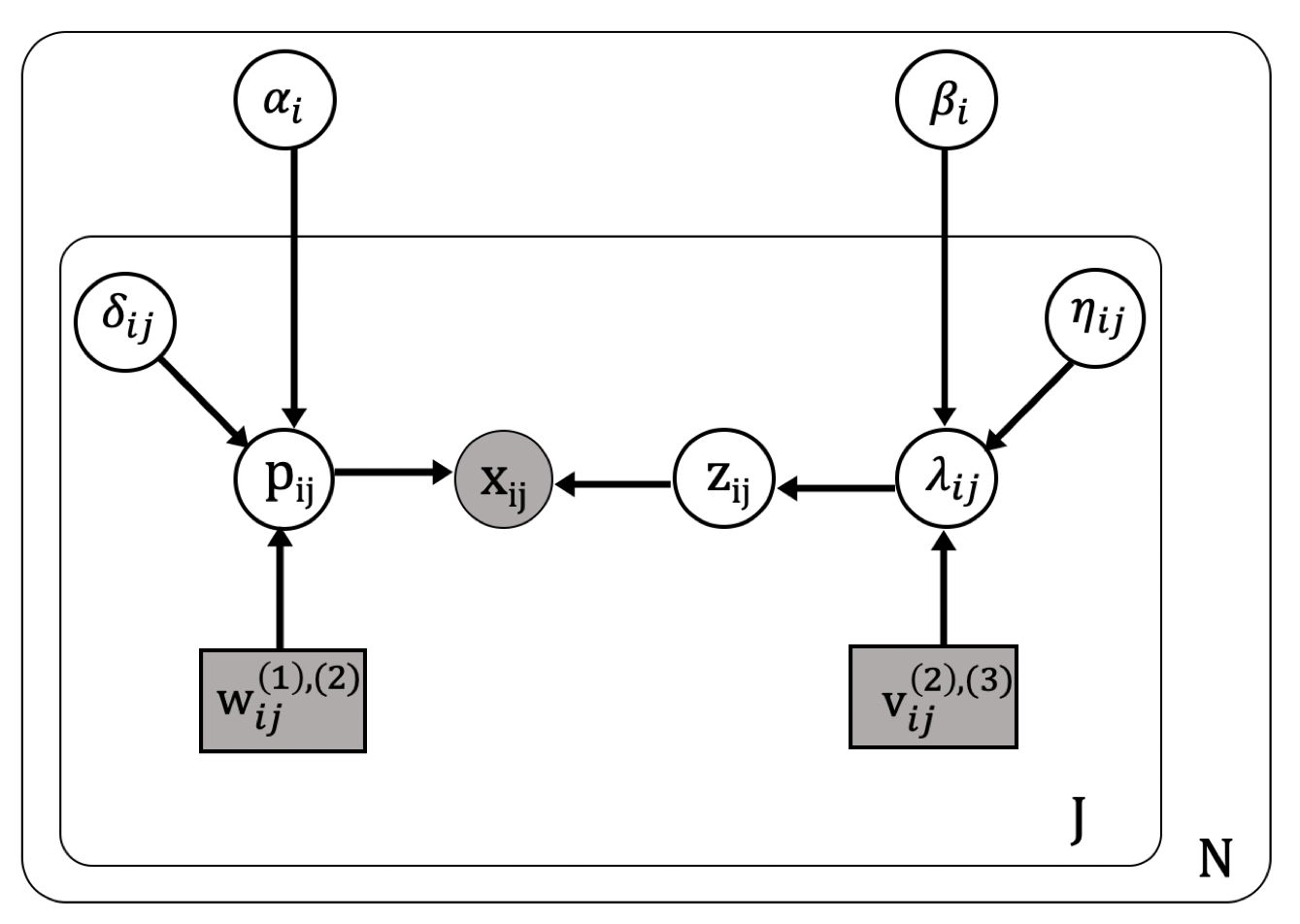
In the model in Section 4, coefficients and are global, encouraging the sharing of information across schools, while school-level terms and capture local properties of individual schools. This model structure is a compromise between complete pooling, in which no school-level differences are permitted ( and omitted), and no pooling, in which each school is modeled separately from all others, with its own coefficient vectors and .
In the case of complete pooling or no pooling, the observed counts still arise from a binomial distribution,
but the true number of assaults and probability of reporting are constructed differently.
C.1 Complete Pooling
The complete pooling scenario assumes that sexual assault reporting patterns do not systematically differ across schools, except to the extent accounted for by their covariates.
The true number of assaults, , follows a model similar to that of Section 4, but with the school-level offset omitted from Equation 3, that is:
Likewise, the probability of reporting is modeled as in Section 4, but with the school-level offset omitted from Equation 5, that is:
C.2 No Pooling
In the no-pooling scenario, each school is modeled separately.
This model has a separate set of coefficients for each school . Each model has a single intercept rather than separate intercepts for urban, suburban, and rural locations, as each school has a single location and does not allow for this distinction. The school-level offset is omitted; when modeling a single school, the dataset does not provide any information that distinguishes from the intercept . When modeling , we thus replace Equation 3 from the original partial pooling model with:
Each school has a separate set of coefficients . As above, the school-level offset is omitted, as the dataset does not distinguish it from the intercept . Coefficients and are omitted. These coefficients correspond whether a school is a junior college, and whether a school is primarily engaged in religious instruction, respectively. As these are fixed characteristics of a school, the data for a single school do not provide information to help distinguish these coefficients from the intercept . When modeling , we thus replace Equation 5 from the original partial pooling model with:
C.3 Comparison
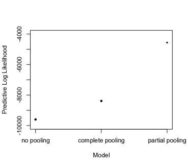
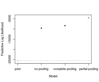
Roughly 20% of records in the campus sexual assault dataset were held out, and posterior inference for the partial pooling, complete pooling, and no pooling models was carried out on the remaining 80% of records. To compare the three models, we approximate the predictive likelihood on the held-out data. Denoting a model’s collection of latent variables as and suppressing covariates, this quantity is
Figure 19 shows that the partial pooling model assigns the highest likelihood to the held-out data. This result that favors the partial pooling model over the two alternatives, as it suggests the partial pooling model does a better job approximating the true distributioin of the data.
 |
 |
| (a) | (b) |
Appendix D Sensitivity to Correlated Reporting
The model in Section 4 assumes that, for a given school in a given year, each assault is reported or not reported independently of all others. In practice, this assumption could plausibly be violated. To explore sensitivity to violations of this assumption, we perform posterior inference on synthetic data with non-independent reporting decisions.
For each school in year , fix the true number of assaults and the reporting probability . Given and , generate a reported number of assaults under different assumptions:
-
•
Independent: For each assault at school in year , assume the reporting decision is independent with probability of reporting.
-
•
=0.05: Assume that each assault at school in year has marginal probability of being reported, but that the reporting decisions are correlated with correlation coefficient , rather than being independent. Simulate this by sampling -many correlated Bernoulli variables, each with probability , and taking their sum to get .
-
•
=0.10: Same as above, but with correlation coefficient .
-
•
Pairwise: Split the total number of assaults at school in year into pairs, and assume that each pair of assaults is reported independently with probability . The marginal reporting probability is still for each assault. This creates correlation in the reporting decisions, but unlike the previous scenario, the amount of correlation varies (schools with a large number of assaults will be less affected by this coarsening of the reported numbers, compared to schools where the true number of assaults is low).
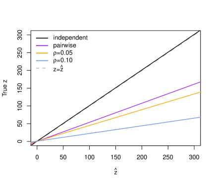
To assess the impact of correlated reporting decisions, we obtain posterior estimates of the true number of assaults for each record in the dataset under each data-generating scenario. For each data-generating scenario, we regress the true number of assaults on the posterior mean estimate . For the dataset simulated with independent reporting decisions, the slope of this regression line is 1.00, indicating that the posterior means of the number of assaults tend to be proportional to the true counts . Figure 20 depicts that the three scenarios with correlated reporting decisions produce slopes less than 1, indicating that the model tends to overestimate the true number of assaults when reporting decisions are positively correlated. This form of model misspecification can significantly degrade the model’s ability to recover the true number of assaults.
Appendix E Sensitivity to Prior Specification
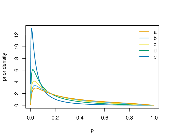
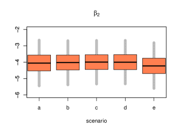
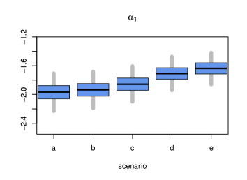
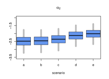
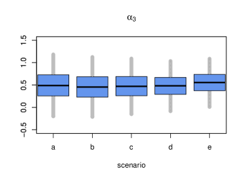
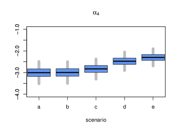
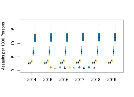
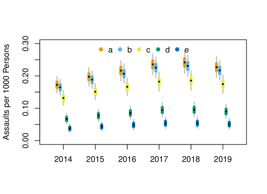
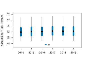
While the National Crime Victimization Survey reflects a significant effort to measure the true extent of sexual assault victimization in the United States, it is nevertheless true that survey respondents may choose not to disclose their sexual assault victimization to interviewers. Consequently, it is worthwhile to examine how a change in the priors informed by NCVS estimates affects the modeling results presented in Section 5. Below we consider a range of alternative scenarios.
-
(a)
Original prior specification presented in Section 4.1-4.2 (Figure 4 and Figure 6).
-
(b)
True reporting rates are approximately 10% lower than NCVS estimates. Prior distributions are adjusted such that the prior median reporting rate is approximately 19.7%, rather than the 22% presented in Section 4.2 (Figure 6). Prior distribution on total incidence of assaults is increased correspondingly.
-
(c)
True reporting rates are approximately 25% lower than estimated by NCVS, with corresponding increase in incidence of assaults.
-
(d)
True reporting rates are approximately 50% lower than estimated by NCVS, with corresponding increase in incidence of assaults.
-
(e)
True reporting rates are approximately 75% lower than estimated by NCVS, with corresponding increase in incidence of assaults.
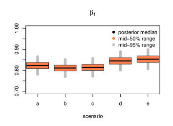
In line with the discussion in Section 4.5, we find that inferences about the role of covariates are relatively more stable across scenarios (as depicted in Figures 22 and 23), while inferences about the true incidence and reporting rate exhibit more sensitivity. As shown in Figure 24, prior belief in a higher incidence of sexual assault produces higher posterior estimates of the total number of assaults occurring. Likewise, Figure 25 demonstrates that prior belief in a lower probability of reporting sexual assault produces lower posterior estimates of the reporting rate. However, zooming in on scenario (e) (which represents the most extreme change to the priors) in Figure 26, results still suggest that an increase in reporting rates is a more plausible explanation for the increase in the increase in reported assaults over 2014-2018, as opposed to an increase in the true incidence of assault. Note that material variability in NCVS survey respondents’ truthfulness over time could call this result into question as well; interested readers may find discussion of a similar issue in the context of marijuana consumption surveys in Cuellar (2018).
 |
 |
| (i) | (ii) |
 |
 |
| (i) | (ii) |
 |
 |
| (iii) | (iv) |
 |
 |
| (i) | (ii) |
Given the sensitivity to prior information, we positively note that in 2011 the Bureau of Justice Statistics convened a panel of statisticians, sociologists, and criminal justice experts to review its methodology and recommend optimal practices for measuring sexual assault (Kruttschnitt, Kalsbeek and House, 2014). The panel’s recommendations led to the development and pilot testing of new survey approaches to measuring sexual assault within the NCVS context (Cantor et al., 2021). These findings fed into a broader multi-year redesign of the overall survey. After further field testing to assess the impact of proposed changes, the redesigned survey is being phased in beginning in 2024 (further detail is available in Truman and Brotsos (2021)).