Oracle-guided Dynamic User Preference Modeling for Sequential Recommendation

Abstract.

Sequential recommendation methods can capture dynamic user preferences from user historical interactions to achieve better performance. However, most existing methods only use past information extracted from user historical interactions to train the models, leading to the deviations of user preference modeling. Besides past information, future information is also available during training, which contains the “oracle” user preferences in the future and will be beneficial to model dynamic user preferences. Therefore, we propose an oracle-guided dynamic user preference modeling method for sequential recommendation (Oracle4Rec), which leverages future information to guide model training on past information, aiming to learn “forward-looking” models. Specifically, Oracle4Rec first extracts past and future information through two separate encoders, then learns a forward-looking model through an oracle-guiding module which minimizes the discrepancy between past and future information. We also tailor a two-phase model training strategy to make the guiding more effective. Extensive experiments demonstrate that Oracle4Rec is superior to state-of-the-art sequential methods. Further experiments show that Oracle4Rec can be leveraged as a generic module in other sequential recommendation methods to improve their performance with a considerable margin.

1. Introduction

Recommender systems, which can recommend potentially interested items to the users according to their historical interactions, have been widely used in various fields, e.g., advertising (Pangesti et al., 2021; Li et al., 2024), movie recommendation (Thakker et al., 2021; Gupta et al., 2020) and E-commerce (Singh and Rishi, 2020; RaviKanth et al., 2019; Bandyopadhyay and Thakur, 2020). Generally, user interactions are continuous and can be seen as a sequence of user’s interacted items sorted in chronological order, which makes user preferences constantly change over time in nature. Sequential recommendation methods (Kang and McAuley, 2018; Sun et al., 2019; Xia et al., 2022; Zhou et al., 2022; Xia et al., 2021, 2024b) can model dynamic user preferences based on his/her historical interaction sequence and achieve better performance compared with static recommendation algorithms (Mnih and Salakhutdinov, 2007; Sedhain et al., 2015; Berg et al., 2017; Cheng et al., 2016; Xia et al., 2024a).

However, existing sequential recommendation methods are faced with one key challenge. When predicting the next interaction, they only use past information extracted from user interactions that come before the current interaction, which could cause the deviations of dynamic user preference modeling since only using past information is insufficient to capture the dynamics of user preferences (Yuan et al., 2020), and thus hurt the performance of recommendation models. Besides past information, future information, which can be extracted from user interactions that come after the current interaction, is also available in the training. It can be viewed as a type of posterior information containing the “oracle” user preferences in the future and is also beneficial to model dynamic user preferences. Using future information to guide model training on past information can learn forward-looking models, which can better model dynamic user preference and thus improve model performance.

To this end, we propose an oracle-guided dynamic user preference modeling method for sequential recommendation (Oracle4Rec) that leverages future information to guide model training on past information, aiming to learn forward-looking models. Specifically, Oracle4Rec first extracts past information and future information through two separate information encoders respectively. The two encoders have the same architecture, which both have a noise filtering module to filter the noise in the user interaction sequence, followed by a causal self-attention module to capture the evolution of user preferences, making the extracted information more accurate. Then Oracle4Rec learns the forward-looking model through a carefully designed oracle-guiding module in a manner of minimizing the discrepancy between past information and future information. To make the guiding from future information to past information more effective, we also tailor a two-phase model training strategy, named 2PTraining, for Oracle4Rec. Extensive experiments on six real-world datasets demonstrate that Oracle4Rec consistently outperforms state-of-the-art sequential recommendation algorithms. We further implement Oracle4Rec as a generic module due to it is orthogonal to existing sequential methods, and we conduct a generality experiment to show that Oracle4Rec has high generality and it can be flexibly applied to other sequential methods and improve their performance with a considerable margin.

The contributions of this work are summarized as follows:

1. We propose an oracle-guided dynamic user preference modeling method for sequential recommendation that can learn forward-looking models through a carefully designed oracle-guiding module and a tailored training strategy, so as to better model dynamic user preferences.

2. We conduct extensive experiments on six public datasets, and the results show that Oracle4Rec achieves better performance compared with other state-of-the-art sequential methods.

3. We implement Oracle4Rec  as a generic module due to it is orthogonal to existing sequential methods, and experiments show that it can improve the performance of those methods with a considerable margin.

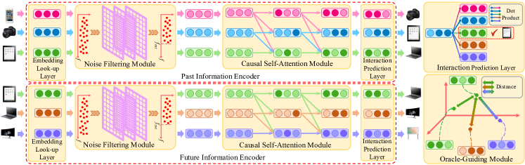
Figure 1. The architecture of Oracle4Rec, which consists of three parts: Past Information Encoder, Future Information Encoder and Oracle-Guiding Module. The first two encoders are both composed of Embedding Look-up Layer, Noise Filtering Module, Causal Self-Attention Module and Interaction Prediction Layer. For the ease of presentation, the Oracle-Guiding Module is set to minimize the distance between past information and future information in a 3D coordinate system.

2. The Proposed Method

2.1. Notations

Let user set and item set be $\mathcal{U}$ and $\mathcal{V}$ respectively, $|\mathcal{U}|=m$ and $|\mathcal{V}|=n$. The user $u$’s interaction sequence in chronological order can be denoted as $\mathcal{S}^{u}=\{v_{i}|v_{i}\in\mathcal{V},i=1,2,\cdots,|\mathcal{S}^{u}|\}$. Our goal is to predict next item $v_{|\mathcal{S}^{u}|+1}$ that user $u$ will interact with based on his/her interaction sequence $\mathcal{S}^{u}$. For the convenience of the following description, we give the definitions of two kinds of user interaction sequences. For a target interaction $v_{t}\in\mathcal{V}$ that needs to be predicted for user $u$, his/her historical interaction sequence can be defined as $\mathcal{H}^{u}_{t}=\{v_{1},v_{2},\cdots,v_{t-1}\}$, and his/her global interaction sequence is defined as $\mathcal{G}^{u}_{t}=\{v_{1},v_{2},\cdots,v_{t-1},v_{t},v_{t+1},\cdots,v_{t+P}\}$, which additionally contains $P+1$ items compared with user historical interaction sequence. We usually adopt fixed-length historical interaction sequence and global interaction sequence for high efficiency during training and inference, thus we need to truncate or pad the sequences $\mathcal{H}^{u}_{t}$ and $\mathcal{G}^{u}_{t}$ to ensure their lengths are equal to a positive integer $L(L>P)$. If the length of sequence is longer than $L$, we truncate its length to $L$ by selecting the recent $L$ interactions, while if the length of sequence is shorter than $L$, we repeatedly add a padding item to the left side of sequence until its length is $L$. Therefore, we redefine the historical interaction sequence as $\mathcal{H}^{u}_{t}=\{v_{t-L},v_{t-L+1},\cdots,v_{t-1}\}$ and the global interaction sequence as $\mathcal{G}^{u}_{t}=\{v_{t+P-L+1},v_{t+P-L+2},\cdots,v_{t+P}\}$.

2.2. Overview of Oracle4Rec

Oracle4Rec is a sequential recommendation method that leverages past information and future information to jointly model dynamic user preferences and make recommendation. Figure 1 shows the architecture of the proposed Oracle4Rec, which consists of three key components: a Past Information Encoder used to extract past information from user historical interaction sequences, a Future Information Encoder used to extract future information from user global interaction sequences, and an Oracle-Guiding Module used to guide model training on past information with future information. We also tailor an effective model training strategy 2PTraining to facilitate the guiding from future information to past information, thereby making past information capture the dynamics of user preferences more accurately and sufficiently. Next, we introduce these modules and the tailored training strategy in details.

2.3. Past Information Encoder

2.3.1. Embedding Look-up Layer

Embedding Look-up Layer is used to generate item embedding matrix $\mathbf{E}^{u}\in\mathbb{R}^{L\times d}$ according to the user historical interaction sequence $\mathcal{H}^{u}_{t}$ by looking up the item embedding table $\mathbf{T}\in\mathbb{R}^{|\mathcal{V}|\times d}$. However, unlike GRU (Cho et al., 2014) and LSTM (Hochreiter and Schmidhuber, 1997), which can capture the order relation between items in the sequence, the attention mechanism in the following Causal Self-Attention Module will ignore it, affecting the accuracy of the dynamic user preference modeling. Therefore, we introduce the positional embedding $\mathbf{E}^{P}\in\mathbb{R}^{L\times d}$ to help the model to identify the order relation between different items. There are many choices of positional embedding, such as sinusoidal positional embedding (Vaswani et al., 2017) and learnable positional embedding (Devlin et al., 2018), we follow the suggestion in (Kang and McAuley, 2018) to use learnable positional embedding for better performance. Thus, the final item embedding is:

(1) $$\hat{\mathbf{E}}^{u}=\mathbf{E}^{u}+\mathbf{E}^{P}.$$

Note that we will take user $u$’s historical sequence $\mathcal{H}^{u}_{t}$ as an example to illustrate how past information encoder works. Thus, we will omit the superscript of all embeddings that are associated with user $u$ for simplicity hereinafter.

2.3.2. Noise Filtering Module

User interaction sequence will inevitably introduce some noisy interactions due to the first impression (Wang et al., 2021), such as caption bias (Hofmann et al., 2012) and position bias (Jagerman et al., 2019), which will cause deviations in modeling user preferences. Specifically, the self-attention mechanism employed in the Causal Self-Attention Module (Section 2.3.3) is highly sensitive to noisy interactions, and the distribution of attention within the model is easily influenced by these noisy interactions, resulting in certain biases in the extracted information. To mitigate the impact of noisy interactions on modeling user dynamic preference, we introduce a Noise Filtering Module before the Causal Self-Attention Module. This adjustment reduces the influence of noisy interactions on modeling user dynamic preference, thereby improving the accuracy of user future interaction predictions.

In the signal processing field, researchers usually analyze and reduce the noise of time series signal in the frequency domain (Duhamel and Vetterli, 1990). Specifically, the time series signal is first transformed from time domain to frequency domain through Fourier transform, so as to obtain a series of frequency components. Generally, noise corresponds to high-frequency components (Yu and Qin, 2020). By eliminating a certain proportion of high-frequency components, we can achieve noise reduction of the signal. Then we transform the signal to time domain through inverse Fourier transform, and we obtain a noise-free time series signal. FMLP-Rec (Zhou et al., 2022) designs a learnable filter to attenuate the noise in the item embedding by imitating the above process. However, the learnable filter may introduce additional model parameters and increase the difficulty of model training.

Since noise corresponds to the high-frequency components and our goal is to remove the noise in the item embedding. Thus, we design the Noise Filtering Module to remove high-frequency components in the item embedding to achieve noise reduction. The noise filtering module has multiple layers, each layer contains a parameter-free low-pass filter to specify how many low-frequency components are preserved. Concretely, in the $g$-th layer, we first transform the item embedding $\mathbf{F}^{g-1}$ from time domain to the frequency domain through the Fast Fourier Transform (FFT):

(2) $$\mathbf{X}^{g}~{},\mathbf{f}^{g}\leftarrow\text{FFT}(\mathbf{F}^{g-1}),$$

where $\mathbf{F}^{g-1}$ is the item embedding from the $(g-1)$-th layer and $\mathbf{F}^{0}=\hat{\mathbf{E}}$, $\mathbf{X}^{g}\in\mathbb{C}^{c\times d}$ and $\mathbf{f}^{g}\in\mathbb{R}^{c}$ are the spectrum matrix and frequency vector respectively, $c$ is the number of frequency components. The cutoff frequency $f_{cut}^{g}$ can be obtained by calculating the $q$ quantile of $\mathbf{f}^{g}$. Then the indicator matrix $\mathbf{M}^{g}\in\mathbb{R}^{c\times d}$ , which decides whether the frequency components are preserved or removed, can be calculated as:

(3) $$\mathbf{M}^{g}=\underbrace{\left[\vmathbb{1}_{\mathbf{f}^{g}_{1}<f_{cut}^{g}},\vmathbb{1}_{\mathbf{f}^{g}_{2}<f_{cut}^{g}},\cdots,\vmathbb{1}_{\mathbf{f}^{g}_{c}<f_{cut}^{g}}\right]^{T}}_{\text{contains }c\text{ elements}}\otimes\mathbf{1}^{T},$$

where $\vmathbb{1}$ is an indicator function, $\mathbf{1}$ is a $d$-dimensional vector whose elements are all 1 and $\otimes$ is the outer product. The filtered spectrum $\tilde{\mathbf{X}}^{g}$ can be obtained by an element-wise product of $\mathbf{X}^{g}$ and $\mathbf{M}^{g}$:

(4) $$\tilde{\mathbf{X}}^{g}=\mathbf{X}^{g}\odot\mathbf{M}^{g}.$$

Then we can get the item embedding after noise reduction through the Inverse Fast Fourier Transform (IFFT). Meanwhile, we incorporate the skip connection (He et al., 2016), layer normalization (Ba et al., 2016) and dropout (Srivastava et al., 2014) to stabilize training. Thus , the final item embedding $\mathbf{F}^{g}$ is

(5) $$\mathbf{F}^{g}=\text{LayerNorm}(\text{Dropout}(\text{IFFT}(\tilde{\mathbf{X}}^{g}))+\mathbf{F}^{g-1}).$$

After $G$ layers, the output of noise filtering module is $\mathbf{F}$.

2.3.3. Causal Self-Attention Module

Compared with RNNs, attention mechanism has surprising long-range dependency modeling ability (Guo et al., 2021; Tang et al., 2018). Therefore, we use the self-attention mechanism, which borrows from (Kang and McAuley, 2018), to construct the Causal Self-Attention Module, so as to capture the dynamic user preferences after reducing the noise in the item embedding. The causal self-attention module is also composed of multiple layers. In the $k$-th layer, the item embedding $\mathbf{S}^{k-1}$ is first fed into a self-attention layer to capture the global information for all items in the sequence:

(6) $$\begin{split}\mathbf{Z}^{k}&=\text{Softmax}({(\mathbf{S}^{k-1}\mathbf{W}^{k}_{Q})(\mathbf{S}^{k-1}\mathbf{W}^{k}_{K})^{T}}/{\sqrt{d}}),\\ \tilde{\mathbf{O}}^{k}&=\mathbf{Z}^{k}(\mathbf{S}^{k-1}\mathbf{W}^{k}_{V}),\\ \mathbf{O}^{k}&=\text{LayerNorm}(\text{Dropout}(\tilde{\mathbf{O}}^{k}\mathbf{W}^{k}_{1}+\mathbf{b}^{k}_{1})+\mathbf{S}^{k-1}),\end{split}$$

where $\mathbf{W}^{k}_{Q}$, $\mathbf{W}^{k}_{K}$ and $\mathbf{W}^{k}_{V}$ are queries, keys and values projection matrices, and $\mathbf{W}^{k}_{1}$ and $\mathbf{b}^{k}_{1}$ are weight and bias of linear transformation at $k$-th layer. Skip connection, layer normalization and dropout are used to stabilize training. $\mathbf{S}^{k-1}$ is the item embedding in the $(k-1)$-th layer and $\mathbf{S}^{0}=\mathbf{F}$. Note that self-attention mechanism does not guarantee the causality that requires the former items cannot receive information from the latter items. Violating the causality will prevent model from learning useful feature and have bad performance in inference. Therefore, when calculating $\mathbf{Z}^{k}$ in Eq. (6), we should set $\mathbf{Z}^{k}_{ij}$ to 0 if $i<j(i,j=1,2,\cdots,n)$.

Then we apply a feed-forward network to the item embedding $\mathbf{O}^{k}$ to capture the non-linearity in the embedding:

(7) $$\mathbf{H}^{k}=\sigma(\mathbf{O}^{k}\mathbf{W}^{k}_{2}+\mathbf{b}^{k}_{2})\mathbf{W}^{k}_{3}+\mathbf{b}^{k}_{3},$$

where $\mathbf{W}^{k}_{2}$, $\mathbf{W}^{k}_{3}$, $\mathbf{b}^{k}_{2}$ and $\mathbf{b}^{k}_{3}$ are weights and biases, $\sigma(\cdot)$ is the activation function. We also incorporate the skip connection, layer normalization and dropout to stabilize training:

(8) $$\mathbf{S}^{k}=\text{LayerNorm}(\text{Dropout}(\mathbf{H}^{k})+\mathbf{O}^{k}).$$

After $K$ layers, we denote the output of this module as $\mathbf{S}$.

2.3.4. Interaction Prediction Layer

After obtaining the predicted item embedding $\mathbf{S}$, we can calculate the probability $P(v_{t}|\mathcal{H}^{u}_{t})$ of the target interaction $v_{t}$ based on $\mathcal{H}^{u}_{t}$ as:

(9) $$P(v_{t}|\mathcal{H}^{u}_{t})=\text{Sigmoid}(\mathbf{Q}_{L}^{T}\mathbf{T}_{v_{t}}),$$

where $\mathbf{Q}_{L}$ is the predicted embedding of the target interaction, which corresponds to the last row of $\mathbf{Q}$, $\mathbf{T}_{v_{t}}$ is the real embedding of the target interaction from embedding table $\mathbf{T}$. Therefore, the loss function of past information encoder is:

(10) $$\small\textstyle\mathcal{L}_{p}=-\sum_{u=1}^{|\mathcal{U}|}\sum_{t=1}^{|\mathcal{S}^{u}|}\left[\log(P(v_{t}|\mathcal{H}^{u}_{t}))+\log(1-P(j|\mathcal{H}^{u}_{t}))\right],$$

where $\mathcal{S}^{u}$ is user $u$’s interaction sequence, and $j\notin\mathcal{S}^{u}$ is a negative item that user $u$ has never interacted with.

2.4. Future Information Encoder

Future information encoder is used to encode the user future preferences from user global interaction sequence. It has the same structure as the past information encoder, which consists of embedding look-up layer, noise filtering module, causal self-attention module and interaction prediction layer. Different from BERT4Rec (Sun et al., 2019), GRec (Yuan et al., 2020) and DualRec (Zhang et al., 2022) that adopt the reversed user interaction sequence to extract future information, i.e., in a Right-to-Left-style, our future information encoder extracts future information in a more natural way, i.e., in a Left-to-Right-style. Given user $u$’s global interaction sequence $\mathcal{G}^{u}_{t}$, the future information encoder outputs the item embedding $\mathbf{R}$. Then we can calculate the probability $P(v_{t+P+1}|\mathcal{G}^{u}_{t})$ of the interaction $v_{t+P+1}$:

(11) $$P(v_{t+P+1}|\mathcal{G}^{u}_{t})=\text{Sigmoid}(\mathbf{R}_{L}^{T}\mathbf{T}_{v_{t+P+1}}),$$

where $\mathbf{R}_{L}$ is the predicted embedding of item $v_{t+P+1}$ and it is the last row of $\mathbf{R}$, $\mathbf{T}_{v_{t+P+1}}$ is the real embedding of item $v_{t+P+1}$ from embedding table $\mathbf{T}$, and $P$ is the number of future interactions after the target interaction $v_{t}$ in $\mathcal{G}^{u}_{t}$. However, the loss function of future information encoder is slightly different from that of past information encoder. Since we want to incorporate future information to make user preference modeling more accurate, we should ensure that future information is sufficiently extracted from user global interaction sequence. Therefore, we use the following loss function to optimize the future information encoder:

(12) $$\mathcal{L}_{f}=-\sum_{u=1}^{|\mathcal{U}|}\sum_{t=1}^{|\mathcal{S}^{u}|}\left[\log(P(\mathcal{G}^{u}_{t+1}|\mathcal{G}^{u}_{t}))+\log(1-P(\mathcal{J}|\mathcal{G}^{u}_{t}))\right]$$

$$=-\sum_{u=1}^{|\mathcal{U}|}\sum_{t=1}^{|\mathcal{S}^{u}|}\sum_{l=1}^{L}\left[\log(P(v_{m+l}|\mathcal{G}^{u}_{t,l}))+\log(1-P(j_{l}|\mathcal{G}^{u}_{t,l}))\right],$$

where $\mathcal{G}^{u}_{t+1}=\{v_{t+P-L+2},v_{t+P-L+3},\cdots,v_{t+P+1}\}$ is user $u$’s global interaction sequence at $t+1$. $\mathcal{J}=\{j_{1},j_{2},\cdots,j_{L}\}$ is the negative item sequence containing $L$ negative items that user has never interact with. $\mathcal{G}^{u}_{t,l}=\{v_{m},v_{m+1},\cdots,v_{m+l-1}\}$ is an sub-sequence of $\mathcal{G}^{u}_{t}$ and $m=t+P-L+1$.

We share the item embedding and positional embedding between past information encoder and future information encoder, which can bring us two benefits: (1) ensure the consistency of item features between encoders, making the model training stable; (2) reduce the number of trainable parameters for easier model training.

2.5. Oracle-Guiding Module

Oracle-Guiding Module is designed to use the future information, as a type of posterior knowledge, to guide the past information to capture the dynamics of user preferences in the future, thereby correcting the deviations in user preference modeling caused by merely using past information. Given two user interaction sequences $\mathcal{H}^{u}_{t}$ and $\mathcal{G}^{u}_{t}$, we can obtain two item embeddings $\mathbf{Q}$ and $\mathbf{R}$ from past and future information encoder respectively. Our goal is to minimize the discrepancy between the predicted embedding of target interaction $v_{t}$ from past information encoder, i.e., $\mathbf{Q}_{L}$ (past information) and the predicted embeddings of the item $v_{t}$ and the following $P+1$ items from future information encoder, i.e., $\mathbf{R}_{L-P-2+i}~{}(i=1,2,\cdots,P+2)$ (future information), making the former embedding can capture how user preferences change in the future through the latter embeddings. Thus, the loss function of oracle-guiding module is:

(13) $$\textstyle\mathcal{L}_{g}=\sum_{i=1}^{P+2}\alpha_{i}\cdot f(\mathbf{Q}_{L},\mathbf{R}_{L-P-2+i}),$$

where $\alpha_{i}\in(0,1]$ is a weight used to distinguish the importance of the $P+2$ discrepancies. Generally, the guiding should pay more attention to the future information near the target interaction $v_{t}$ and pay less attention to the future information far away from $v_{t}$, therefore we use exponential attenuation to model $\alpha_{i}$:

(14) $$\alpha_{i}=\text{e}^{-\gamma(i-1)},$$

where $\gamma$ is the attenuation coefficient. Since $\mathbf{Q}_{L}$ and $\mathbf{R}_{L-P-1}$ corresponds to the same item $v_{t}$, the discrepancy $f(\mathbf{Q}_{L},\mathbf{R}_{L-P-1})$ has the highest importance, thus the weight $\alpha_{1}$ is 1. $f(\cdot)$ is a discrepancy measurement function. There are many choices to model $f(\cdot)$, we introduce four commonly used choices, including Kullback-Leibler divergence (KL divergence), Jensen–Shannon Divergence (JS Divergence), Euclidean distance and Cosine distance. Note that for KL divergence and JS Divergence, we need to use the Softmax function to transform $\mathbf{Q}$ and $\mathbf{R}$ to the probabilistic distributions first. We choose KL divergence in Oracle4Rec since it achieves the best performance in empirical studies.

2.6. 2PTraining: A Tailored Training Strategy

Traditional training, which jointly trains past and future information encoder, is unsuitable for Oracle4Rec since joint training will make the past and future information be extracted simultaneously, weakening the guiding effect of future information. Thus, we tailor an effective two-phase model training strategy 2PTraining, which first trains the future information encoder with the loss $\mathcal{L}_{f}$ to obtain future information, then jointly trains past information encoder and oracle-guiding module with the loss $\mathcal{L}_{p}+\beta\mathcal{L}_{g}$ to obtain past information and achieve guiding from future information to past information, to facilitate learning of forward-looking models. We leave the algorithm of 2PTraining in the Appendix due to the space limitation. The experimental results demonstrate the superiority of 2PTraining compared with traditional training strategy.

2.7. Inference

In the inference phase, the future information is not available, thus we only use past information encoder to predict the items that users will interact with. Given user $u$’s historical interaction sequence $\mathcal{H}^{u}_{t}$, we first use past information encoder to obtain the predicted item embedding $\mathbf{Q}\in\mathbb{R}^{L\times d}$. Since we want to predict which item $v\in\mathcal{V}$ user $u$ will interact with after interacting the item $v_{t-1}$, we can first calculate the interaction score $s^{u}_{t,v}$, and then the item with the highest score can be seen as the predicted item $v_{t}$ that user will be interested to interact with:

(15) $$\textstyle s^{u}_{t,v}=\mathbf{Q}_{L}^{T}\mathbf{T}_{v},\quad v_{t}=\underset{v\in\mathcal{V}}{\arg\max}~{}s^{u}_{t,v}.$$

2.8. Discussions

2.8.1. Rationality of Adopting Future Information.

Intuitively, the current prediction can be more accurate when taking future uncertainty into account, since future information, as a kind of hindsight observations, can server as a regularizer to narrow down the representation learning space so as to enhance the accuracy of representation learning and correct the impact of some noisy interactions on user/item representation learning. In deep reinforcement learning, researchers adopt hindsight observation to improve the quality of representation learning (Guez et al., 2020; Fang et al., 2021). For instance, OPD (Fang et al., 2021) trained a teacher network with hindsight information, and employed network distillation to facilitate the learning of student network for stock trading. Inspired by this, we design the oracle-guiding module with the hope that future observations can guide and facilitate the current user preference modeling, thereby more accurately predicting user future interactions.

2.8.2. Differences Between Oracle4Rec and Existing Methods.

Though Oracle4Rec, DualRec and GRec adopt past and future information to model dynamic user preferences, there are five major differences between them, and we leave the detailed comparison in the Appendix due to the space limitation: (1) The future information extraction manner is different. DualRec and GRec adopts a right-to-left manner while Oracle4Rec adopts a left-to-right manner. (2) The future information utilization process is different. DualRec and GRec learns and utilizes future information simultaneously, whereas Oracle4Rec first learns future information and then utilizes it to guide model training. (3) The solution to noisy interactions is different. DualRec and GRec do not consider the impact of noisy interactions on modeling user preference, while Oracle4Rec proposes a lightweight noise filtering module to deal with noisy interactions. (4) The training target for future information encoder is different. DualRec uses the same loss function for both past and future information encoders, while Oracle4Rec redesigns the future information encoder’s loss function (Eq.(LABEL:eq:fae_loss)) by considering the guiding role of future information. (5) The treatment of future information across periods is different. DualRec treats future information across periods equally while Oracle4Rec treats them selectively by assigning them respective weights when narrowing the gap between future and past information.

2.8.3. Comparison between Embedding Alignment and Mask & Prediction.

The Mask & Prediction technique is commonly used in the NLP domain (Devlin et al., 2018) to infer the embedding of a masked word based on its contextual information. BERT4Rec (Sun et al., 2019) inherits this training paradigm and applies it to recommendation algorithms, aiming to infer masked interactions from user interaction sequences. However, we anticipate that current interaction may not always be accurately inferred from future interactions. Therefore, we propose to use the embedding alignment technique, which employs two independent encoders to encode past and future information separately. We use future information to guide model learning on past information. In this training paradigm, our goal is not to infer the current interaction from its context but to regularize the learning of past information using future information, thereby enhancing the consistency of the two types of information. This helps prevent learning spurious correlations, ultimately improving the coherence and accuracy of user preferences modeling.

Moreover, when user interaction sequence exhibits a degree of randomness and noise, it is more challenging for Mask & Prediction technique to infer current interaction from future ones. However, encoding user features to capture future changes and guiding model learning on past features are relatively straightforward.

Table 1. The statistics of the six real-world datasets.

	ML100K	ML1M	Beauty	Sports	Toys	Yelp
# Users	943	6,040	22,363	25,598	19,412	30,431
# Items	1,349	3,416	12,101	18,357	11,924	20,033
# Interactions	99,287	999,611	198,052	296,337	167,597	316,354
Density	7.805%	4.485%	0.073%	0.063%	0.072%	0.052%

Table 2. Performance comparison on six datasets. The best result is denoted in bold, the second best result is denoted with an underline. The “$\star$” denotes the statistical significance ($p$ ¡ 0.05) of the results of Oracle4Rec compared to the strongest baseline.

Datasets	Metrics	PopRec	GRU4Rec	Caser	RepeatNet	HGN	CLEA	SASRec	BERT4Rec	GRec	SRGNN	GCSAN	FMLP-Rec	DualRec	Oracle4Rec
ML100K	HR@1	0.0859	0.1737	0.1680	0.1773	0.1513	0.1741	0.1926	0.1786	0.1669	0.1834	0.2040	0.2085	0.2097	0.2257⋆
	HR@5	0.2397	0.4795	0.4676	0.4732	0.4427	0.4783	0.5005	0.4829	0.4468	0.4806	0.4993	0.5224	0.4993	0.5330⋆
	NDCG@5	0.1619	0.3300	0.3220	0.3296	0.2971	0.3294	0.3499	0.3349	0.3117	0.3370	0.3581	0.3705	0.3579	0.3843⋆
	HR@10	0.3669	0.6566	0.6473	0.6431	0.6036	0.6615	0.6653	0.6361	0.6348	0.6585	0.6664	0.6783	0.6670	0.6908⋆
	NDCG@10	0.2024	0.3872	0.3801	0.3846	0.3514	0.3897	0.4034	0.3846	0.3729	0.3946	0.4121	0.4208	0.4108	0.4353⋆
	MRR	0.1771	0.3205	0.3144	0.3211	0.2891	0.3211	0.3381	0.3243	0.3098	0.3291	0.3489	0.3562	0.3481	0.3706⋆
ML1M	HR@1	0.0904	0.3132	0.3119	0.3530	0.2404	0.3203	0.3478	0.3375	0.3448	0.3404	0.3648	0.3541	0.3482	0.3709⋆
	HR@5	0.3002	0.6576	0.6375	0.6547	0.5644	0.6557	0.6803	0.6632	0.6327	0.6474	0.6694	0.6830	0.6557	0.7106⋆
	NDCG@5	0.1964	0.4962	0.4848	0.5138	0.4104	0.5128	0.5255	0.5114	0.4978	0.5034	0.5272	0.5294	0.5116	0.5531⋆
	HR@10	0.4416	0.7754	0.7585	0.7651	0.7087	0.7658	0.7889	0.7716	0.7460	0.7567	0.7773	0.7916	0.7727	0.8128⋆
	NDCG@10	0.2420	0.5345	0.5236	0.5498	0.4572	0.5486	0.5608	0.5467	0.5337	0.5389	0.5623	0.5648	0.5496	0.5863⋆
	MRR	0.2038	0.4689	0.4607	0.4923	0.3922	0.4911	0.4982	0.4857	0.4784	0.4811	0.5042	0.5024	0.4901	0.5228⋆
Beauty	HR@1	0.0678	0.1599	0.1304	0.1613	0.1609	0.1327	0.1794	0.1684	0.1317	0.1777	0.1985	0.2038	0.2182	0.2199⋆
	HR@5	0.2105	0.3565	0.3054	0.3287	0.3531	0.3310	0.3880	0.3586	0.2868	0.3650	0.3792	0.4089	0.4103	0.4317⋆
	NDCG@5	0.1391	0.2627	0.2211	0.2482	0.2608	0.2344	0.2886	0.2674	0.2127	0.2753	0.2932	0.3117	0.3192	0.3316⋆
	HR@10	0.3386	0.4596	0.4072	0.4239	0.4544	0.4425	0.4885	0.4598	0.3826	0.4662	0.4707	0.5079	0.5029	0.5295⋆
	NDCG@10	0.1803	0.2960	0.2539	0.2789	0.2934	0.2704	0.3211	0.3000	0.2435	0.3078	0.3227	0.3436	0.3490	0.3632⋆
	MRR	0.1558	0.2633	0.2264	0.2524	0.2616	0.2378	0.2865	0.2689	0.2209	0.2768	0.2940	0.3092	0.3178	0.3278⋆
Sports	HR@1	0.0763	0.1291	0.1024	0.1325	0.1444	0.1254	0.1503	0.1405	0.1055	0.1473	0.1674	0.1699	0.1831	0.1861⋆
	HR@5	0.2293	0.3397	0.2834	0.3208	0.3484	0.3397	0.3672	0.3466	0.2786	0.3498	0.3702	0.3915	0.4031	0.4191⋆
	NDCG@5	0.1538	0.2372	0.1947	0.2290	0.2492	0.2327	0.2620	0.2463	0.1937	0.2517	0.2721	0.2846	0.2981	0.3070⋆
	HR@10	0.3423	0.4635	0.4061	0.4381	0.4698	0.4623	0.4964	0.4730	0.3948	0.4738	0.4909	0.5137	0.5267	0.5431⋆
	NDCG@10	0.1902	0.2772	0.2342	0.2668	0.2883	0.2750	0.3037	0.2870	0.2315	0.2916	0.3111	0.3240	0.3380	0.3471⋆
	MRR	0.1660	0.2391	0.2028	0.2342	0.2522	0.2504	0.2632	0.2496	0.2027	0.2552	0.2743	0.2833	0.2980	0.3037⋆
Toys	HR@1	0.0585	0.1481	0.1114	0.1370	0.1541	0.1245	0.1799	0.1504	0.1069	0.1682	0.1995	0.1926	0.2170	0.2152
	HR@5	0.1977	0.3456	0.2944	0.3007	0.3430	0.3278	0.3652	0.3446	0.2687	0.3572	0.3787	0.4007	0.4043	0.4233⋆
	NDCG@5	0.1286	0.2505	0.2054	0.2213	0.2516	0.2286	0.2766	0.2504	0.1891	0.2661	0.2926	0.3015	0.3149	0.3246⋆
	HR@10	0.3008	0.4532	0.4052	0.4007	0.4485	0.4421	0.4609	0.4567	0.3694	0.4605	0.4740	0.5032	0.4999	0.5222⋆
	NDCG@10	0.1618	0.2852	0.2411	0.2535	0.2857	0.2643	0.3075	0.2866	0.2219	0.2995	0.3234	0.3346	0.3458	0.3565⋆
	MRR	0.1430	0.2517	0.2107	0.2279	0.2542	0.2313	0.2778	0.2531	0.1983	0.2680	0.2942	0.2994	0.3153	0.3215⋆
Yelp	HR@1	0.0801	0.2109	0.1858	0.2344	0.2337	0.2085	0.2276	0.2446	0.1711	0.2400	0.2561	0.2704	0.2817	0.2970⋆
	HR@5	0.2415	0.5772	0.5170	0.5360	0.5663	0.5678	0.5856	0.5848	0.4743	0.5772	0.5932	0.6231	0.6272	0.6499⋆
	NDCG@5	0.1622	0.3998	0.3560	0.3897	0.4057	0.3842	0.4117	0.4203	0.3251	0.4147	0.4301	0.4538	0.4610	0.4812⋆
	HR@10	0.3609	0.7474	0.6866	0.6950	0.7306	0.7488	0.7651	0.7514	0.6567	0.7398	0.7557	0.7777	0.7839	0.8000⋆
	NDCG@10	0.2007	0.4552	0.4110	0.4411	0.4589	0.4465	0.4699	0.4744	0.3837	0.4675	0.4829	0.5040	0.5119	0.5300⋆
	MRR	0.1740	0.3770	0.3409	0.3778	0.3885	0.3669	0.3915	0.4017	0.3176	0.3966	0.4113	0.4299	0.4393	0.4562⋆

3. Experiments

3.1. Experimental Setup

We adopt six widely used datasets to comprehensively evaluate the performance of Oracle4Rec: (1) ML100K and ML1M (two movie datasets) (Harper and Konstan, 2015). (2) Beauty, Sports and Toys (three product datasets) (He and McAuley, 2016b; McAuley et al., 2015). (3) Yelp (a business dataset) (Asghar, 2016). To make a fair comparison, for all datasets, we group the interaction records by users, and sort them ascendingly in chronological order. Besides, we follow FMLP-Rec to filter unpopular items and inactive users with fewer than five interactions. We also adopt the same dataset split, which is commonly used in sequential recommendation, as FMLP-Rec, i.e., the last item of each user interaction sequence for test, the penultimate item for validation, and all remaining items for training. Table 1 describes the statistics of the six datasets.

We compare Oracle4Rec with 13 sequential methods. (1) PopRec; (2) GRU4Rec (Hidasi et al., 2015); (3) Caser (Tang and Wang, 2018); (4) HGN (Ma et al., 2019); (5) RepeatNet (Ren et al., 2019); (6) CLEA (Qin et al., 2021); (7) SASRec (Kang and McAuley, 2018); (8) BERT4Rec (Sun et al., 2019); (9) GRec (Yuan et al., 2020); (10) SRGNN (Wu et al., 2019); (11) GCSAN (Xu et al., 2019); (12) FMLP-Rec (Zhou et al., 2022); and (13) DualRec (Zhang et al., 2022). For all methods, BERT4Rec, GRec and DualRec can access the future information, while other methods can merely use past information for user preference modeling.

We compare Oracle4Rec with other methods in top-K recommendation task with three popular ranking metrics: (1) Hit Ratio (HR); (2) Normalized Discounted Cumulative Gain (NDCG); and (3) Mean Reciprocal Rank (MRR). For the former two metrics, we report their results when K=1, 5, 10, i.e., HR@{1, 5, 10} and NDCG@{1, 5, 10}, and we omit NDCG@1 since it is equal to HR@1. For a fair comparison, we follow the same negative sampling strategy as FMLP-Rec to pair the ground-truth item with 99 randomly sampled negative items that the user has not interacted with.

We adopt Adam optimizer (Kingma and Ba, 2014) to optimize the model with learning rates $\eta_{1}=\eta_{2}=0.001$, we set the maximum sequence length $L$ to 50 and the number of future interactions $P$ in user global interaction sequence to 10. For all datasets, we tune hidden size $d$ from [32, 64, 128, 256], attenuation coefficient $\gamma$ from 0.005 to 1.0, frequency quantile $q$ from 0.3 to 1.0 and regularization coefficient $\beta$ from [0.005, 0.01, 0.05]. Dropout probabilities are fixed to 0.5. We also tune the layer number of noise filtering module from 1 to 3 and the layer number of causal self-attention module from 1 to 5. The hyper-parameters of all baselines are carefully tuned according to their papers. Due to the space limitation, we leave the detailed setup in the Appendix.

3.2. Performance Comparison

Table 2 shows performance comparison of all methods. Following FMLP-Rec, we also report the full-ranking results, i.e., ranking the ground-truth item with all candidate items, in the Appendix. From the results, we have the following observations:

1. Transformer-based methods (i.e., SASRec and Bert4Rec) achieve better accuracy than RNN-based methods (i.e., GRU4Rec and HGN) and CNN-based methods (i.e., Caser). The main reason is that the self-attention mechanism in Transformer-based methods has the largest receptive field compared with RNNs and CNNs, so it can capture more information from user interaction sequence, which can make user preference modeling more precise.

2. GNN-based methods (i.e., SRGNN and GCSAN) have comparable or better performance than Transformer-based methods. This is because the GNN has a powerful structure feature extraction ability (Xu et al., 2018), and can capture the transition relationship between items, so as to achieve more accurate recommendation results.

3. FMLP-Rec and DualRec achieve better accuracy than all other baselines. This is because the former has strong noise reduction capability to filter the noise in the user interactions, and the latter can utilize both past information and future information from user interactions, making them model user preference more accurate.

4. Oracle4Rec consistently outperforms all compared methods on all datasets, demonstrating its superiority. Compared with methods only using past information, Oracle4Rec effectively leverages past and future information in training, making the dynamic user preference modeling more accurate. Compared with BERT4Rec, GRec and DualRec, Oracle4Rec adopts an oracle-guiding module and a 2PTraining to leverage future information in a more effective way, thus achieving better performance. Generally, using future information can reduce the error of predicting user’s interested items during training, and thus will make more accurate recommendation. This can be drawn by comparing the losses, which is placed in the Appendix due to the space limitation, when Oracle4Rec uses past information only or past and future information together.

Table 3. Ablation study of Oracle4Rec on ML100K, ML1M and Beauty datasets. Bold face indicates the highest performance.

	ML100K			ML1M			Beauty
	HR@1	NDCG@5	MRR	HR@1	NDCG@5	MRR	HR@1	NDCG@5	MRR
(1) Oracle4Rec w/o Noise Filtering Module	0.1909	0.3554	0.3443	0.3658	0.5495	0.5189	0.2062	0.3104	0.3090
(2) Oracle4Rec w/ Learnable Filter	0.2042	0.3637	0.3513	0.3523	0.5262	0.4995	0.2087	0.3121	0.3110
(3) Oracle4Rec w/o Future Information Encoder	0.1782	0.3391	0.3277	0.3477	0.5275	0.4993	0.1878	0.3010	0.2975
(4) Oracle4Rec w/o Attenuation of Discrepancies	0.1983	0.3604	0.3491	0.3347	0.5225	0.4924	0.2123	0.3255	0.3217
(5) Oracle4Rec w/ Traditional Training Strategy	0.2087	0.3670	0.3566	0.3497	0.5302	0.5016	0.2041	0.3164	0.3129
(6) Oracle4Rec w/ JS Diverge	0.1968	0.3583	0.3456	0.3555	0.5399	0.5095	0.2160	0.3257	0.3222
(7) Oracle4Rec w/ Euclidean Distance	0.1987	0.3622	0.3491	0.3630	0.5445	0.5149	0.2071	0.3194	0.3158
(8) Oracle4Rec w/ Cosine Distance	0.2070	0.3712	0.3572	0.3608	0.5439	0.5137	0.2078	0.3211	0.3172
(9) Oracle4Rec Future Information Encoder	0.1911	0.3407	0.3328	0.3283	0.5063	0.4798	0.1986	0.3017	0.3004
(10) Oracle4Rec w/ R2L-style	0.2078	0.3659	0.3549	0.3389	0.5157	0.4892	0.2071	0.3174	0.3148
(11) Oracle4Rec (w/ KL Divergence & L2R-style)	0.2257	0.3843	0.3706	0.3709	0.5531	0.5228	0.2199	0.3316	0.3278

Table 4. The KL divergence between user real and predicted preference under different settings on ML100K and ML1M.

	ML100K	ML1M
Oracle4Rec w/o Future Information Encoder	0.0085	0.0069
Oracle4Rec w/ Future Information Encoder	0.0070 (+17.6%)	0.0062 (+10.1%)

3.3. Ablation Study

We conduct the extensive ablation study to comprehensively analyze the impact of each component on the performance of Oracle4Rec. Table 3 shows the results. Due to the space limitation, the results of other metrics are placed in the Appendix.

1. Comparing setting (1) and (11), we can find that without the noise filtering module, the performance of Oracle4Rec significantly decreases on all cases. This is because user interactions are inevitably noisy. By reducing the noise in the interaction sequence using low-pass filter, Oracle4Rec can more accurately model user preferences, thus making more accurate recommendations. Comparing setting (2) and (11), the results show that low-pass filter (setting (11)) achieves better results than learnable filter, which we attribute to the additional parameters of learnable filter increase the difficulty of model training, thus reducing the performance.

2. Comparing setting (3) and (11), we can find that Oracle4Rec obtains better accuracy than Oracle4Rec w/o Future Information Encoder, which shows the importance of oracle information guiding in model training, i.e., punish deviations from user future preferences. Moreover, merely using future information encoder can also lead to sub-optimal performance by comparing setting (9) and (11). Therefore, we can conclude that guiding from future information to past information can make user preference modeling more reliable.

3. The attenuation in the oracle-guiding module is helpful to improve the model performance by comparing setting (4) and (11). This is because with attenuation, Oracle4Rec can selectively minimize the discrepancies between past and future information from different time, thus capturing the evolution of user preferences and achieving better performance.

4. We can find that 2PTraining is beneficial to improve the performance of Oracle4Rec by comparing setting (5) and (11). Traditional training strategy jointly trains past and future information encoders, which is unable to sufficiently leverage past information and future information. However, 2PTraining first optimizes future information encoder then optimizes the past information encoder, making the model able to fully leverage these two information.

5. Comparing setting (6)–(8) and (11), we can find that the performance of Oracle4Rec varies with different discrepancy measurement methods. When equipped with KL divergence, Oracle4Rec achieves the best results. Thus, we adopt KL divergence as the discrepancy measurement method in Oracle4Rec.

6. The L2R-style (left-to-right-style) information extraction manner is superior than the R2L-style (right-to-left-style) information extraction manner by comparing setting (10) and (11), which demonstrates the rationality of our left-to-right-style. Generally, the left-to-right-style is more intuitive and aligns with the chronological order of interactions, making the extracted information more sufficient and the modeled user preference more accurate.

3.4. Future Information Encoder Analysis

To explore how future information encoder can facilitate the learning process of Oracle4Rec, or in other words, what Oracle4Rec will learn when equipped with future information encoder, we analyze the consistency of user real preference and user predicted preference on ML100K and ML1M. The former preference is calculated from the categories of real items that user interacts with in the inference phase, which is denoted as $p$, and the latter preference is calculated from the categories of top-10 items predicted by Oracle4Rec w/o future information encoder and Oracle4Rec w/ future information encoder, denoted as $q^{(1)}$ and $q^{(2)}$. By comparing the KL divergence $\mathbf{KL}(p,q^{(1)})$ and $\mathbf{KL}(p,q^{(2)})$, we can determine whether future information encoder benefits the learning process of Oracle4Rec. We leave the details about the calculation of preference and KL divergence in the Appendix due to the space limitation.

Table 4 shows the experimental results. We can observe that the KL divergence is reduced when Oracle4Rec is equipped with future information encoder, which demonstrates that future information encoder can make predicted items more similar to items that user will interact with in terms of item categories and is beneficial to the leaning process of Oracle4Rec. Generally, future information encoder can help infer “oracle” user preference in the future, and with the help of oracle-guiding module, Oracle4Rec can recognize how user preference will change from past to future, which cannot be achieved by merely using past information encoder, thus making user dynamic preference modeling more accurate.

Figure 2 shows four preference distributions of two randomly selected users on ML100K. More cases are placed in the Appendix. Note that historical distribution is calculated from the categories of items that user has interacted with in the training phase. From the results, we can find that merely using past information will make the model easily overfit historical preference. For instance, items related to category 2 have higher probability to be recommended to user 260 than other categories, making the model overfit this category by comparing historical distribution and distribution from PIE. Same phenomenon can be found in the category 3 and 5 of user 869. However, with future information encoder, the probabilities of those categories are reduced by comparing distribution from PIE and distribution from Oracle4Rec, alleviating the overfiting issue. Moreover, future information encoder makes the predicted preference distribution closer to the real distribution by comparing real distribution, distribution from PIE and distribution from Oracle4Rec, e.g., category 1 and 2 for user 260 and category 3—6 for user 869, leading to more accurate user interaction prediction.

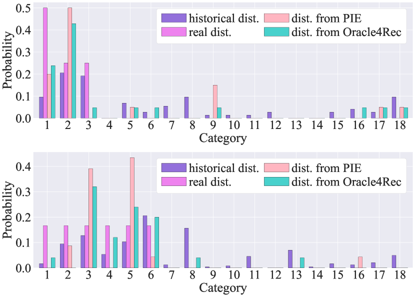
Figure 2. Four preference distributions of user 260 (the upper figure) and 869 (the lower figure) on ML100K. “dist.” means distribution, and “PIE” is past information encoder, i.e., Oracle4Rec w/o Future information Encoder.

3.5. Generality Analysis

We apply the oracle-guiding module and 2PTraining of Oracle4Rec into four sequential methods GRU4Rec, SRGNN, GCSAN and FMLP-Rec and evaluate their performance afterwards to further analyze the generality of Oracle4Rec. Table 5 shows the results, the results of other metrics are placed in the Appendix. We can find that the performance of all methods has a significant improvement, which shows Oracle4Rec has high generality. The results also show that leveraging future information can improve the performance of sequential methods, since future information as a type of posterior knowledge contains the evolution of user preferences in the future, which can address the deviations caused by only using past information to model dynamic user preferences as GRU4Rec, SRGNN, GCSAN and FMLP-Rec do, thus achieving superior performance.

Table 5. Generality analysis of four sequential methods. “XYZ+” means applying Oracle4Rec into the corresponding method XYZ. Bold face indicates better performance in that group. The “$\star$” denotes the statistical significance ($p$ ¡ 0.05) of the results of XYZ+ compared to XYZ.

	ML100K			ML1M
	HR@1	NDCG@5	MRR	HR@1	NDCG@5	MRR
GRU4Rec	0.1737	0.3300	0.3205	0.3132	0.4962	0.4689
GRU4Rec+	0.2059⋆	0.3642⋆	0.3532⋆	0.3446⋆	0.5244⋆	0.4964⋆
SRGNN	0.1834	0.3370	0.3291	0.3404	0.5034	0.4811
SRGNN+	0.1985⋆	0.3574⋆	0.3466⋆	0.3578⋆	0.5244⋆	0.5006⋆
GCSAN	0.2040	0.3581	0.3489	0.3648	0.5272	0.5042
GCSAN+	0.2159⋆	0.3741⋆	0.3613⋆	0.3846⋆	0.5462⋆	0.5231⋆
FMLP-Rec	0.2085	0.3705	0.3562	0.3541	0.5294	0.5024
FMLP-Rec+	0.2178⋆	0.3788⋆	0.3658⋆	0.3657⋆	0.5396⋆	0.5125⋆

3.6. Sensitivity Analysis

We analyse how Oracle4Rec performs with respect to three important hyper-parameters number of future interactions, frequency quantile and attenuation coefficient on Beauty. However, due to the space constraints, we leave experimental results in the Appendix.

4. Related Work

Sequential recommendation methods model dynamic user preferences according to his/her historical interactions (Ma et al., 2019; Ren et al., 2019; Qin et al., 2021). Several techniques have been applied in this line of work, from the earliest Markov Chain (Rendle et al., 2010; He and McAuley, 2016a), to the later Recurrent Neural Networks (Wu et al., 2017; Hidasi et al., 2015), Convolutional Neural Networks (Tuan and Phuong, 2017; Tang and Wang, 2018), Self-Attention Mechanism (Kang and McAuley, 2018; Sun et al., 2019) and Graph Neural Networks (Wu et al., 2019; Xu et al., 2019). FPMC (Rendle et al., 2010) is a Markov Chain-based sequential method that combines Markov chain and matrix factorization to model user preferences. Fossil (He and McAuley, 2016a) fuses the similarity-based method with Markov Chain to characterize users in terms of both preferences and the strength of sequential behavior, addressing the sparsity issues and the long-tailed distribution of datasets. Due to the vigorous development of deep learning, the performance of sequential recommendation methods has been significantly improved. GRU4Rec (Hidasi et al., 2015) adopts GRU (Cho et al., 2014) to model the dynamic user preferences. 3D-CNN (Tuan and Phuong, 2017) uses a convolutional neural network to capture sequential patterns and model user preference. SASRec (Kang and McAuley, 2018) uses a self-attention mechanism (Vaswani et al., 2017) to capture user long-term preferences. SRGNN (Wu et al., 2019) and GCSAN (Xu et al., 2019) are GNN-based sequential methods that use graph neural networks (Scarselli et al., 2008; Kipf and Welling, 2016) and self-attention mechanism to model user preferences. FMLP-Rec (Zhou et al., 2022) adopts an all-MLP architecture to model dynamic user preferences. Note that contrastive learning based sequential methods are another line of works, they are different from ours, thus we exclude them.

However, the above methods only use the past information to make recommendation, making the model performance sub-optimal. Future information is also available during training and is beneficial to model user preferences. BERT4Rec (Sun et al., 2019), GRec (Yuan et al., 2020) and DualRec (Zhang et al., 2022) are three sequential methods that integrates past and future information to model dynamic user preferences. Though Oracle4Rec also leverages future information to model dynamic user preferences, there are several major differences between existing methods and Oracle4Rec, as discussed in Section 2.8.2.

5. Conclusion

We propose an oracle-guided dynamic user preference modeling method for sequential recommendation that uses future information to guide model training on past information, so as to better model dynamic user preferences. Oracle4Rec first extracts past and future information through two separate encoders, then learns forward-looking models through an oracle-guiding module and a tailored model training strategy. Extensive experimental results demonstrate the superiority of Oracle4Rec. The generality experiment further shows that Oracle4Rec can be flexibly applied to other sequential methods and greatly improve their performance.

Ethical Considerations

To the best of our knowledge, this work does not bring new negative societal impacts, including fairness, privacy, security, safety, misuse of the technology by malicious actors, as well as possible harms that could arise even when the technology is being used as intended and functioning correctly.

Appendix A Additional Details of Oracle4Rec

A.1. The Algorithm of 2PTraining

Algorithm 1 shows the workflow of the 2PTraining. At first, 2PTraining randomly initializes model parameters (line 1). Then for each epoch, 2PTraining first trains the future information encoder (line 3–4), followed by a forward propagation to obtain the sufficiently encoded future information (line 5), and then trains the past information encoder and oracle-guiding module to achieve the guiding from future information to past information (line 6–8).

Algorithm 1 The workflow of 2PTraining.

Input: User historical interaction sequence $\mathcal{H}^{u}_{t}$, user global interaction sequence $\mathcal{G}^{u}_{t}$, learning rates $\eta_{1}$ and $\eta_{2}$, number of training epochs $I$, regularization coefficient $\beta$.

Parameters: Parameters of past information encoder $\mathbf{\Theta}_{p}$, parameters of future information encoder $\mathbf{\Theta}_{f}$.

1:  Randomly initialize $\mathbf{\Theta}_{p}$ and $\mathbf{\Theta}_{f}$.

2:  for $i=1,\cdots,I$ do

3:     Train the future information encoder with $\mathcal{G}^{u}_{t}$ to obtain $\mathcal{L}_{f}$.

4:     Update parameters $\mathbf{\Theta}_{f}$ using gradient descent:$\mathbf{\Theta}_{f}\leftarrow\mathbf{\Theta}_{f}-\eta_{1}\frac{\partial\mathcal{L}_{f}}{\partial\mathbf{\Theta}_{f}}$.

5:     Feed forward $\mathcal{G}^{u}_{t}$ into the future information encoder once and obtain future information $\mathbf{R}$

6:     Train the past information encoder with $\mathcal{H}^{u}_{t}$ to obtain past information $\mathbf{Q}$ and loss $\mathcal{L}_{p}$.

7:     Train the Oracle-Guiding Module with $\mathbf{Q}$ and $\mathbf{R}$ and obtain the loss $\mathcal{L}_{g}$.

8:     Update parameters $\mathbf{\Theta}_{p}$ using gradient descent:$\mathbf{\Theta}_{p}\leftarrow\mathbf{\Theta}_{p}-\eta_{2}\frac{\partial(\mathcal{L}_{p}+\beta\cdot\mathcal{L}_{g})}{\partial\mathbf{\Theta}_{p}}$.

9:  end for

A.2. The detailed differences between Oracle4Rec and existing methods

Though both Oracle4Rec, DualRec and GRec adopt past information and future information to model dynamic user preferences, there are five major differences between them:

1. DualRec and GRec extract future information from user interaction sequences in a right-to-left manner, while Oracle4Rec extracts future information in a left-to-right manner. The latter is more intuitive, aligning with the chronological order of interactions, where the usage of items should follow the sequence of interactions.

2. DualRec and GRec employ joint training of past and future information encoders to learn user dynamic preferences, whereas Oracle4Rec first trains a future information encoder to encode future information and then trains a past encoder to guide the model training through future information. We believe that simultaneously training both encoders in the former may lead to mutual interference between them, causing instability and inadequacy in feature learning. In contrast, the two-stage training approach in the latter can avoid mutual interference, resulting in more stable feature learning and more effective utilization of future information.

3. DualRec does not consider the impact of noisy interactions on modeling user dynamic preferences, while Oracle4Rec addresses the issue of widespread noise in user interaction sequences by introducing a lightweight (no trainable parameters) noise filtering module. This module reduces the impact of noisy interactions on modeling user preferences without adding a burden to the model training.

4. DualRec uses the same loss function for both past and future information encoders, extracting past and future information from user interaction sequences. In contrast, Oracle4Rec, considering the guiding role of future information, redesigns the encoder’s loss function (Equation 12). This ensures accurate and comprehensive encoding of future information from user interaction sequences, guiding model learning on past information and ensuring the coherence of user preference changes.

5. DualRec treats future information from different time equally when narrowing the gap between future and past information, without considering the varying importance of future information at different time. In Oracle4Rec, the narrowing of the gap is selectively applied. Specifically, future information closer to the current time has a more significant impact on guidance at the current time. Therefore, larger weights should be assigned when reducing the gap. In contrast, future information from the current time has a less significant impact, so smaller weights should be assigned when narrowing the gap. This selective approach in Oracle4Rec results in user preferences with higher coherence and accuracy.

Appendix B Additional Details of experimental Setup

B.1. Datasets

We adopt six widely used datasets to comprehensively evaluate the performance of Oracle4Rec: (1) ML100K and ML1M are two popular movie recommendation datasets collected by GroupLens Research from the MovieLens web site. (2) Beauty, Sports and Toys are three product recommendation datasets collected from Amazon.com. (3) Yelp is a business recommendation dataset. We only use the user interaction records after January 1st, 2019 since it is a very large dataset.

To make a fair comparison, for all datasets, we group the interaction records by users, and sort them ascendingly in chronological order. Besides, we follow (Hidasi et al., 2016; Rendle et al., 2010) to filter unpopular items and inactive users with fewer than five interaction records. We also adopt the same dataset split as FMLP-Rec (Zhou et al., 2022), i.e., the last item of each user interaction sequence for test, the penultimate item for validation, and all remaining items for training.

B.2. Compared Methods

We compare Oracle4Rec with the following 13 sequential recommendation methods.

1. PopRec is a simple method that ranks items based on the item popularity.

2. GRU4Rec (Hidasi et al., 2015) uses GRU to model dynamic user preferences.

3. Caser (Tang and Wang, 2018) adopts horizontal and vertical convolutions to model user short-term preferences.

4. HGN (Ma et al., 2019) integrates a hierarchical gating network with the BPR (Rendle et al., 2012) to capture both long-term and short-term user interests.

5. RepeatNet (Ren et al., 2019) uses an encoder-decoder structure that can choose items from a user’s history and recommends them at the right time through a repeat recommendation mechanism.

6. CLEA (Qin et al., 2021) uses contrastive learning technique to automatically extract items relevant to the target item for recommendation.

7. SASRec (Kang and McAuley, 2018) uses a self-attention mechanism to capture user long-term preferences based on relatively few actions.

8. BERT4Rec (Sun et al., 2019) employs a bidirectional self-attention to model user behavior sequences.

9. GRec (Yuan et al., 2020) integrates past information and future information through a gap-filling mechanism.

10. SRGNN (Wu et al., 2019) models user interaction sequences as a session graph and uses GNN and Attention Network to capture dynamic user preferences.

11. GCSAN (Xu et al., 2019) is a state-of-the-art method that uses GNN and Self-Attention Mechanism to model dynamic user preferences over a session graph generated from user interaction sequences.

12. FMLP-Rec (Zhou et al., 2022) is a state-of-the-art method that adopts an all-MLP structure with learnable filters to filter the noise in user interaction sequences and model accurate user preferences.

13. DualRec (Zhang et al., 2022) proposed a dual network to achieve past-future disentanglement and past-future mutual enhancement, so as to alleviate the training-inference gap.

B.3. Metrics

We compare Oracle4Rec with other state-of-the-art sequential recommendation methods in top-K recommendation task with three kinds of popular ranking metrics: (1) Hit Ratio (HR), which evaluates the coincidence of user recommendation list and ground-truth interaction list; (2) Normalized Discounted Cumulative Gain (NDCG), which accumulates the gains from ranking list with the discounted gains at lower ranks; (3) Mean Reciprocal Rank (MRR), which evaluates the performance of ranking according to the harmonic mean of the ranks. Note that for the former two metrics, we report their results when K=1, 5, 10, that is HR@{1, 5, 10} and NDCG@{1, 5, 10}, and we omit NDCG@1 metric since it is equal to HR@1. For a fair comparison, we follow the same negative sampling strategy as FMLP-Rec (Zhou et al., 2022) to pair the ground-truth item with 99 randomly sampled negative items that the user has not interacted with.

Table 6. Performance comparison on six datasets. The best result is denoted in bold, the second best result is denoted with an underline. The “$\star$” denotes the statistical significance ($p$ ¡ 0.05) of the results of Oracle4Rec compared to the strongest baseline.

Datasets	Metrics	GRU4Rec	RepeatNet	HGN	SASRec	BERT4Rec	GCSAN	FMLP-Rec	DualRec	Oracle4Rec
ML100K	HR@1	0.0993	0.1046	0.0855	0.0886	0.1101	0.1241	0.1184	0.1214	0.1317⋆
	HR@5	0.0619	0.0677	0.0527	0.0695	0.0710	0.0794	0.0753	0.0792	0.0867⋆
	NDCG@5	0.1637	0.1784	0.1427	0.1767	0.1771	0.1968	0.1930	0.1833	0.2083⋆
	HR@10	0.0826	0.0911	0.0711	0.0917	0.0926	0.1026	0.0992	0.0972	0.1112⋆
	NDCG@10	0.2623	0.2785	0.2195	0.2762	0.2825	0.2952	0.2471	0.2661	0.3086⋆
	MRR	0.1074	0.1162	0.0903	0.1166	0.1190	0.1274	0.1134	0.1194	0.1364⋆
ML1M	HR@1	0.1116	0.1311	0.0817	0.1339	0.1331	0.1565	0.1361	0.1470	0.1613⋆
	HR@5	0.0705	0.0857	0.0512	0.0865	0.0851	0.1026	0.0884	0.1004	0.1062⋆
	NDCG@5	0.1864	0.2034	0.1348	0.2106	0.2105	0.2330	0.2153	0.2116	0.2456⋆
	HR@10	0.0945	0.1088	0.0682	0.1111	0.1099	0.1275	0.1138	0.1212	0.1334⋆
	NDCG@10	0.2894	0.2863	0.2114	0.3147	0.3152	0.3249	0.2735	0.2956	0.3569⋆
	MRR	0.1204	0.1314	0.0874	0.1373	0.1363	0.1512	0.1292	0.1423	0.1614⋆
Beauty	HR@1	0.0183	0.0365	0.0321	0.0361	0.0324	0.0451	0.0403	0.0403	0.0526⋆
	HR@5	0.0113	0.0255	0.0203	0.0232	0.0209	0.0311	0.0260	0.0287	0.0347⋆
	NDCG@5	0.0329	0.0537	0.0528	0.0561	0.0527	0.0653	0.0653	0.0556	0.0784⋆
	HR@10	0.0159	0.0311	0.0269	0.0296	0.0274	0.0376	0.0340	0.0336	0.0430⋆
	NDCG@10	0.0564	0.0777	0.0817	0.0837	0.0794	0.0927	0.0838	0.0772	0.1132⋆
	MRR	0.0202	0.0371	0.0343	0.0366	0.0341	0.0445	0.0389	0.0390	0.0517⋆
Sports	HR@1	0.0110	0.0174	0.0176	0.0187	0.0156	0.0227	0.0247	0.0252	0.0285⋆
	HR@5	0.0071	0.0116	0.0112	0.0124	0.0098	0.0154	0.0162	0.0168	0.0186⋆
	NDCG@5	0.0181	0.0277	0.0296	0.0294	0.0257	0.0345	0.0379	0.0394	0.0440⋆
	HR@10	0.0094	0.0149	0.0150	0.0158	0.0130	0.0192	0.0204	0.0212	0.0236⋆
	NDCG@10	0.0300	0.0424	0.0464	0.0449	0.0414	0.0505	0.0479	0.0600	0.0665⋆
	MRR	0.0124	0.0186	0.0192	0.0197	0.0169	0.0232	0.0231	0.0265	0.0293⋆
Toys	HR@1	0.0217	0.0333	0.0303	0.0462	0.0305	0.0573	0.0526	0.0561	0.0625⋆
	HR@5	0.0142	0.0245	0.0206	0.0312	0.0205	0.0419	0.0355	0.0394	0.0420
	NDCG@5	0.0352	0.0466	0.0479	0.0676	0.0476	0.0784	0.0774	0.0794	0.0891⋆
	HR@10	0.0185	0.0288	0.0262	0.0381	0.0260	0.0486	0.0435	0.0470	0.0506⋆
	NDCG@10	0.0558	0.0643	0.0717	0.0931	0.0710	0.1043	0.0947	0.1083	0.1223⋆
	MRR	0.0237	0.0332	0.0322	0.0445	0.0320	0.0552	0.0480	0.0542	0.0589⋆
Yelp	HR@1	0.0120	0.0155	0.0151	0.0150	0.0163	0.0211	0.0182	0.0211	0.0233⋆
	HR@5	0.0076	0.0097	0.0094	0.0094	0.0099	0.0132	0.0113	0.0134	0.0147⋆
	NDCG@5	0.0211	0.0268	0.0263	0.0256	0.0292	0.0350	0.0314	0.0357	0.0393⋆
	HR@10	0.0105	0.0133	0.0130	0.0128	0.0141	0.0177	0.0155	0.0180	0.0198⋆
	NDCG@10	0.0364	0.0452	0.0446	0.0423	0.0496	0.0575	0.0429	0.0584	0.0655⋆
	MRR	0.0143	0.0179	0.0176	0.0170	0.0191	0.0233	0.0186	0.0235	0.0263⋆

B.4. Implementation Details

We implement our method using PyTorch. We adopt Adam optimizer (Kingma and Ba, 2014) to optimize the model with learning rates $\eta_{1}=\eta_{2}=0.001$, we set the maximum sequence length $L$ to 50 and the number of future interactions $P$ in user global interaction sequence to 10. For all datasets, we tune hidden size $d$ from [32, 64, 128, 256], attenuation coefficient $\gamma$ from 0.005 to 1.0, frequency quantile $q$ from 0.3 to 1.0 and regularization coefficient $\beta$ from [0.005, 0.01, 0.05]. Dropout probabilities are fixed to 0.5. We also tune the layer number of noise filtering module from 1 to 3 and the layer number of causal self-attention module from 1 to 5.

We also implement all baselines expect PopRec, CLEA , GRec, FMLP-Rec and DualRec based on a comprehensive and efficient recommendation library RecBole (Zhao et al., 2022). For CLEA, GRec, FMLP-Rec and DualRec, we directly use their released code. For a fair comparison, we adopt the same data preprocessing, training and inference procedures as FMLP-Rec. We carefully tune the model hyper-parameters according to their original papers and report the best results.

Appendix C Additional Results of Performance Comparison in Full-Ranking Setting

Following FMLP-Rec (Zhou et al., 2022), we select GRU4Rec, RepeatNet, HGN, SASRec, BERT4Rec, GCSAN, FMLP-Rec and DualRec as representative compared methods and HR@{5, 10, 20} and NDCG@{5, 10, 20} as metrics to further verify the effectiveness of Oracle4Rec under full-ranking setting, which ranks the ground-truth item with all candidate items. Table 6 shows the results, and we can find that Oracle4Rec achieves better performance than other methods, which demonstrates the superiority of Oracle4Rec.

Table 7. Addition results of ablation study of Oracle4Rec on ML100K, ML1M and Beauty datasets. Bold face indicates the highest performance.

	ML100K			ML1M			Beauty
	HR@5	HR@10	NDCG@10	HR@5	HR@10	NDCG@10	HR@5	HR@10	NDCG@10
(1) Oracle4Rec w/o Noise Filtering Module	0.5073	0.6867	0.4136	0.7078	0.8083	0.5822	0.4042	0.5014	0.3418
(2) Oracle4Rec w/ Learnable Filter	0.5143	0.6838	0.4183	0.6772	0.7803	0.5597	0.4052	0.5023	0.3435
(3) Oracle4Rec w/o Future Information Encoder	0.4939	0.6768	0.3984	0.6839	0.7900	0.5621	0.4038	0.5054	0.3339
(4) Oracle4Rec w/o Attenuation of Discrepancies	0.5107	0.6838	0.4164	0.6853	0.7939	0.5579	0.4269	0.5274	0.3582
(5) Oracle4Rec w/ Traditional Training Strategy	0.5139	0.6880	0.4234	0.6877	0.7949	0.5651	0.4180	0.5191	0.3490
(6) Oracle4Rec w/ JS Diverge	0.5088	0.6789	0.4132	0.6999	0.8043	0.5739	0.4245	0.5224	0.3573
(7) Oracle4Rec w/ Euclidean Distance	0.5128	0.6757	0.4151	0.7022	0.8077	0.5788	0.4204	0.5200	0.3516
(8) Oracle4Rec w/ Cosine Distance	0.5224	0.6842	0.4234	0.7028	0.8060	0.5775	0.4224	0.5208	0.3528
(9) Oracle4Rec Future Information Encoder	0.4814	0.6513	0.3959	0.6629	0.7780	0.5438	0.3949	0.4894	0.3322
(10) Oracle4Rec w/ R2L-style	0.5122	0.6800	0.4201	0.6689	0.7772	0.5510	0.4158	0.5161	0.3497
(11) Oracle4Rec (w/ KL Divergence & L2R-style)	0.5330	0.6908	0.4353	0.7106	0.8128	0.5863	0.4317	0.5295	0.3632

Appendix D Analysis of Loss in past information encoder

Figure 3 shows the losses of past information encoder when using past information only or past and future information together to model user preferences on ML100K and ML1M datasets. We can find that using future information reduces the error of predicting user’s interested items during training, and thus will make more accurate recommendation in inference.

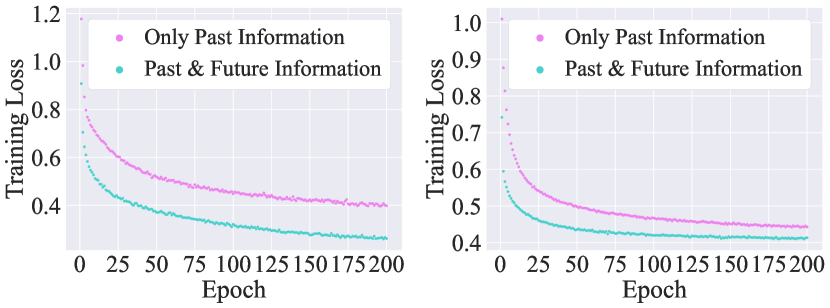
Figure 3. The losses of past information encoder when using past information only or past and future information together on ML100K (left) and ML1M (right) datasets.

Appendix E Additional Results of Ablation Study

Table 7 shows the additional results of ablation study of Oracle4Rec on ML100K, ML1M and Beauty datasets. From the results, we can find that all components of Oracle4Rec, i.e. noise filtering module, future information encoder, attenuation of discrepancies in oracle-guiding module, tailored 2PTraining and the left-to-right-style information extraction manner, have positive impact on the performance of Oracle4Rec, and KL divergence is the most suitable discrepancy measurement method for Oracle4Rec.

Appendix F Additional Results of Future Information Encoder Analysis

F.1. The Calculation of Preference Distribution

We define user $u$’s preference distribution $p_{u}$ according to the categories (e.g., Comedy, Action) of items that are related to user $u$:

(16) $$p_{u}(\text{category}=c)=\frac{A_{uc}}{\sum_{c^{\prime}=1}^{C}A_{c^{\prime}k}},$$

where $A_{uc}~{}(u=1,2,\cdots,M,~{}~{}~{}c=1,2,\cdots,C)$ represents the number of appearances of the $c$-th category in the user $u$’s interacted items, $M$ is the number of users, and $C$ is the number of categories. There are three types of preference distributions used in the experiment:

1. User historical preference distribution, which is calculated from the categories of items that user has interacted with in the training phase.

2. User real preference distribution, which is calculated from the categories of items that user will interact with in the inference phase, which can reflect user real preference in the future.

3. User predicted preference distribution, which is calculated from the categories of top-10 items predicted by the model.

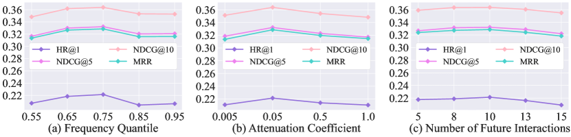
Figure 4. Sensitivity analysis of three important hyper-parameters in Oracle4Rec on Beauty.

F.2. The Calculation of KL Divergence

KL divergence can be used to estimate the consistency of two distributions, thus we use KL divergence to evaluate the quality of the user predicted preference distribution with respect to user real preference distribution, where smaller KL divergence indicates better user predicted preference distribution. The KL divergence between user real preference distribution ($p$) and user predicted preference distribution ($q$) is:

(17) $$\mathbf{KL}(p,q)=\frac{1}{M}\sum_{u=1}^{M}\sum_{c=1}^{C}p_{u}(c)\ln\frac{p_{u}(c)}{q_{u}(c)}.$$

F.3. Additional Cases of User Preference Distributions

Figure 5 and Figure 6 show the additional cases of four preference distributions of six randomly selected users on ML100K and ML1M respectively. From the results, we can find that merely using past information will make the model easily overfit historical preference. However, with the help of future information encoder, the probabilities of those categories are reduced by comparing distribution from PIE and distribution from Oracle4Rec, alleviating the overfiting issue. Moreover, future information encoder makes the predicted preference distribution closer to the real distribution in inference phase by comparing real distribution, distribution from PIE and distribution from Oracle4Rec, leading to more accurate user future interaction prediction.

Table 8. Generality analysis of four sequential methods on ML100K and ML1M datasets. “XYZ+” means applying Oracle4Rec into the corresponding method XYZ. Bold face indicates better performance in that group. The “$\star$” denotes the statistical significance ($p$ ¡ 0.05) of the results of XYZ+ compared to XYZ.

	ML100K			ML1M
	HR@5	HR@10	NDCG@10	HR@5	HR@10	NDCG@10
GRU4Rec	0.4795	0.6566	0.3872	0.6576	0.7754	0.5345
GRU4Rec+	0.5116⋆	0.6793⋆	0.4181⋆	0.6800⋆	0.7901⋆	0.5602⋆
SRGNN	0.4806	0.6585	0.3946	0.6474	0.7567	0.5389
SRGNN+	0.5060⋆	0.6744⋆	0.4119⋆	0.6708⋆	0.7826⋆	0.5606⋆
GCSAN	0.4993	0.6664	0.4121	0.6694	0.7773	0.5623
GCSAN+	0.5228⋆	0.6859⋆	0.4267⋆	0.6864⋆	0.7913⋆	0.5803⋆
FMLP-Rec	0.5224	0.6783	0.4208	0.6830	0.7916	0.5648
FMLP-Rec+	0.5275	0.6904⋆	0.4313⋆	0.6915⋆	0.7968⋆	0.5739⋆

Appendix G Additional Results of Generality Analysis

Table 8 shows the additional results of generality analysis on HR@5, HR@10 and NDCG@10. From the results, we can find that the performance of all methods has a significant improvement, which shows Oracle4Rec has high generality.

Appendix H Results of Sensitivity Analysis

We analyse how Oracle4Rec performs with respect to three important hyper-parameters frequency quantile, number of future interactions and attenuation coefficient on Beauty. Figure 4 shows the results. We neglect HR@5 and HR@10 since their range are different from others, but their trends are the same as others.

Figure 4(a) shows the performance of Oracle4Rec with frequency quantile varying in [0.55, 0.65, 0.75, 0.85, 0.95], and we can observe that when frequency quantile increases, the performance becomes better. This is because more frequency components are preserved, making the user preference modeling more precise. However, when frequency quantile is larger than 0.75, the performance is getting worse. This is because some high-frequency components, which correspond to the noise, are preserved, affecting the user preference modeling and model performance.

Figure 4 (b) shows the performance of Oracle4Rec with attenuation coefficient varying in [0.005, 0.05, 0.5, 1.0]. We can find that with the increase of the attenuation coefficient, all metrics first increase and then decrease. When the attenuation coefficient is too small, Oracle4Rec can not distinguish the importance of features in different periods, making it unable to learn the evolution of user preferences in the future. While when the attenuation coefficient is too large, Oracle4Rec pays too much attention to the features in the near future, but ignores that of the longer term, making the user preferences modeling inadequate.

Figure 4 (c) shows the performance of Oracle4Rec with the number of future interactions varying in [5, 8, 10, 13, 15]. From the results, we can observe that the best performance is achieved when it is 10. When it is too small, future information cannot be extracted from limited user future interactions, resulting in sub-optimal dynamic user preference modeling. When it is too large, excessive future interactions impact the model to extract effective and accurate information, and further impact the guiding of model training on past information, resulting in low performance.

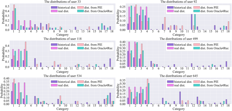
Figure 5. Additional cases of four preference distributions of randomly selected 6 users on ML100K. “dist.” means distribution, and “PIE” is past information encoder, i.e., Oracle4Rec w/o Future information Encoder.

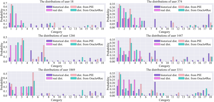
Figure 6. Additional cases of four preference distributions of randomly selected 6 users on ML1M. “dist.” means distribution, and “PIE” is past information encoder, i.e., Oracle4Rec w/o Future information Encoder.

References

- (1)
- Asghar (2016) Nabiha Asghar. 2016. Yelp dataset challenge: Review rating prediction. arXiv preprint arXiv:1605.05362 (2016).
- Ba et al. (2016) Jimmy Lei Ba, Jamie Ryan Kiros, and Geoffrey E Hinton. 2016. Layer normalization. arXiv preprint arXiv:1607.06450 (2016).
- Bandyopadhyay and Thakur (2020) Soma Bandyopadhyay and SS Thakur. 2020. Product prediction and recommendation in e-commerce using collaborative filtering and artificial neural networks: A hybrid approach. In Intelligent Computing Paradigm: Recent Trends. Springer, 59–67.
- Berg et al. (2017) Rianne van den Berg, Thomas N Kipf, and Max Welling. 2017. Graph convolutional matrix completion. arXiv preprint arXiv:1706.02263 (2017).
- Cheng et al. (2016) Heng-Tze Cheng, Levent Koc, Jeremiah Harmsen, Tal Shaked, Tushar Chandra, Hrishi Aradhye, Glen Anderson, Greg Corrado, Wei Chai, Mustafa Ispir, et al. 2016. Wide & deep learning for recommender systems. In Proceedings of the 1st workshop on deep learning for recommender systems. 7–10.
- Cho et al. (2014) Kyunghyun Cho, Bart Van Merriënboer, Caglar Gulcehre, Dzmitry Bahdanau, Fethi Bougares, Holger Schwenk, and Yoshua Bengio. 2014. Learning phrase representations using RNN encoder-decoder for statistical machine translation. arXiv preprint arXiv:1406.1078 (2014).
- Devlin et al. (2018) Jacob Devlin, Ming-Wei Chang, Kenton Lee, and Kristina Toutanova. 2018. Bert: Pre-training of deep bidirectional transformers for language understanding. arXiv preprint arXiv:1810.04805 (2018).
- Duhamel and Vetterli (1990) Pierre Duhamel and Martin Vetterli. 1990. Fast Fourier transforms: a tutorial review and a state of the art. Signal processing 19, 4 (1990), 259–299.
- Fang et al. (2021) Yuchen Fang, Kan Ren, Weiqing Liu, Dong Zhou, Weinan Zhang, Jiang Bian, Yong Yu, and Tie-Yan Liu. 2021. Universal trading for order execution with oracle policy distillation. In Proceedings of the AAAI Conference on Artificial Intelligence, Vol. 35. 107–115.
- Guez et al. (2020) Arthur Guez, Fabio Viola, Théophane Weber, Lars Buesing, Steven Kapturowski, Doina Precup, David Silver, and Nicolas Heess. 2020. Value-driven hindsight modelling. Advances in Neural Information Processing Systems 33 (2020), 12499–12509.
- Guo et al. (2021) Xudong Guo, Xun Guo, and Yan Lu. 2021. Ssan: Separable self-attention network for video representation learning. In Proceedings of the IEEE/CVF Conference on Computer Vision and Pattern Recognition. 12618–12627.
- Gupta et al. (2020) Meenu Gupta, Aditya Thakkar, Vishal Gupta, Dhruv Pratap Singh Rathore, et al. 2020. Movie recommender system using collaborative filtering. In 2020 International Conference on Electronics and Sustainable Communication Systems (ICESC). IEEE, 415–420.
- Harper and Konstan (2015) F Maxwell Harper and Joseph A Konstan. 2015. The movielens datasets: History and context. Acm transactions on interactive intelligent systems (tiis) 5, 4 (2015), 1–19.
- He et al. (2016) Kaiming He, Xiangyu Zhang, Shaoqing Ren, and Jian Sun. 2016. Deep residual learning for image recognition. In Proceedings of the IEEE conference on computer vision and pattern recognition. 770–778.
- He and McAuley (2016a) Ruining He and Julian McAuley. 2016a. Fusing similarity models with markov chains for sparse sequential recommendation. In 2016 IEEE 16th international conference on data mining (ICDM). IEEE, 191–200.
- He and McAuley (2016b) Ruining He and Julian McAuley. 2016b. Ups and downs: Modeling the visual evolution of fashion trends with one-class collaborative filtering. In proceedings of the 25th international conference on world wide web. 507–517.
- Hidasi et al. (2015) Balázs Hidasi, Alexandros Karatzoglou, Linas Baltrunas, and Domonkos Tikk. 2015. Session-based recommendations with recurrent neural networks. arXiv preprint arXiv:1511.06939 (2015).
- Hidasi et al. (2016) Balázs Hidasi, Massimo Quadrana, Alexandros Karatzoglou, and Domonkos Tikk. 2016. Parallel recurrent neural network architectures for feature-rich session-based recommendations. In Proceedings of the 10th ACM conference on recommender systems. 241–248.
- Hochreiter and Schmidhuber (1997) Sepp Hochreiter and Jürgen Schmidhuber. 1997. Long short-term memory. Neural computation 9, 8 (1997), 1735–1780.
- Hofmann et al. (2012) Katja Hofmann, Fritz Behr, and Filip Radlinski. 2012. On caption bias in interleaving experiments. In Proceedings of the 21st ACM international conference on Information and knowledge management. 115–124.
- Jagerman et al. (2019) Rolf Jagerman, Harrie Oosterhuis, and Maarten de Rijke. 2019. To model or to intervene: A comparison of counterfactual and online learning to rank from user interactions. In Proceedings of the 42nd international ACM SIGIR conference on research and development in information retrieval. 15–24.
- Kang and McAuley (2018) Wang-Cheng Kang and Julian McAuley. 2018. Self-attentive sequential recommendation. In 2018 IEEE international conference on data mining (ICDM). IEEE, 197–206.
- Kingma and Ba (2014) Diederik P Kingma and Jimmy Ba. 2014. Adam: A method for stochastic optimization. arXiv preprint arXiv:1412.6980 (2014).
- Kipf and Welling (2016) Thomas N Kipf and Max Welling. 2016. Semi-supervised classification with graph convolutional networks. arXiv preprint arXiv:1609.02907 (2016).
- Li et al. (2024) Dongsheng Li, Jianxun Lian, Le Zhang, Kan Ren, Tun Lu, Tao Wu, and Xing Xie. 2024. Recommender Systems: Frontiers and Practices. Springer Nature.
- Ma et al. (2019) Chen Ma, Peng Kang, and Xue Liu. 2019. Hierarchical gating networks for sequential recommendation. In Proceedings of the 25th ACM SIGKDD international conference on knowledge discovery & data mining. 825–833.
- McAuley et al. (2015) Julian McAuley, Christopher Targett, Qinfeng Shi, and Anton Van Den Hengel. 2015. Image-based recommendations on styles and substitutes. In Proceedings of the 38th international ACM SIGIR conference on research and development in information retrieval. 43–52.
- Mnih and Salakhutdinov (2007) Andriy Mnih and Russ R Salakhutdinov. 2007. Probabilistic matrix factorization. Advances in neural information processing systems 20 (2007).
- Pangesti et al. (2021) Witriana Endah Pangesti, Rachmat Suryadithia, Muhammad Faisal, Bilal Abdul Wahid, Arman Syah Putra, et al. 2021. Collaborative Filtering Based Recommender Systems For Marketplace Applications. International Journal of Educational Research and Social Sciences (IJERSC) 2, 5 (2021), 1201–1209.
- Qin et al. (2021) Yuqi Qin, Pengfei Wang, and Chenliang Li. 2021. The world is binary: Contrastive learning for denoising next basket recommendation. In Proceedings of the 44th International ACM SIGIR Conference on Research and Development in Information Retrieval. 859–868.
- RaviKanth et al. (2019) K RaviKanth, K ChandraShekar, K Sreekanth, and P Santhosh Kumar. 2019. Recommendation system for e-commerce by memory based and model based collaborative filtering. In International Conference on Soft Computing and Pattern Recognition. Springer, 123–129.
- Ren et al. (2019) Pengjie Ren, Zhumin Chen, Jing Li, Zhaochun Ren, Jun Ma, and Maarten De Rijke. 2019. Repeatnet: A repeat aware neural recommendation machine for session-based recommendation. In Proceedings of the AAAI Conference on Artificial Intelligence, Vol. 33. 4806–4813.
- Rendle et al. (2012) Steffen Rendle, Christoph Freudenthaler, Zeno Gantner, and Lars Schmidt-Thieme. 2012. BPR: Bayesian personalized ranking from implicit feedback. arXiv preprint arXiv:1205.2618 (2012).
- Rendle et al. (2010) Steffen Rendle, Christoph Freudenthaler, and Lars Schmidt-Thieme. 2010. Factorizing personalized markov chains for next-basket recommendation. In Proceedings of the 19th international conference on World wide web. 811–820.
- Scarselli et al. (2008) Franco Scarselli, Marco Gori, Ah Chung Tsoi, Markus Hagenbuchner, and Gabriele Monfardini. 2008. The graph neural network model. IEEE transactions on neural networks 20, 1 (2008), 61–80.
- Sedhain et al. (2015) Suvash Sedhain, Aditya Krishna Menon, Scott Sanner, and Lexing Xie. 2015. Autorec: Autoencoders meet collaborative filtering. In Proceedings of the 24th international conference on World Wide Web. 111–112.
- Singh and Rishi (2020) Mahesh Kumar Singh and Om Prakash Rishi. 2020. Event driven recommendation system for E-commerce using knowledge based collaborative filtering technique. Scalable Computing: Practice and Experience 21, 3 (2020), 369–378.
- Srivastava et al. (2014) Nitish Srivastava, Geoffrey Hinton, Alex Krizhevsky, Ilya Sutskever, and Ruslan Salakhutdinov. 2014. Dropout: a simple way to prevent neural networks from overfitting. The journal of machine learning research 15, 1 (2014), 1929–1958.
- Sun et al. (2019) Fei Sun, Jun Liu, Jian Wu, Changhua Pei, Xiao Lin, Wenwu Ou, and Peng Jiang. 2019. BERT4Rec: Sequential recommendation with bidirectional encoder representations from transformer. In Proceedings of the 28th ACM international conference on information and knowledge management. 1441–1450.
- Tang et al. (2018) Gongbo Tang, Mathias Müller, Annette Rios, and Rico Sennrich. 2018. Why self-attention? a targeted evaluation of neural machine translation architectures. arXiv preprint arXiv:1808.08946 (2018).
- Tang and Wang (2018) Jiaxi Tang and Ke Wang. 2018. Personalized top-n sequential recommendation via convolutional sequence embedding. In Proceedings of the eleventh ACM international conference on web search and data mining. 565–573.
- Thakker et al. (2021) Urvish Thakker, Ruhi Patel, and Manan Shah. 2021. A comprehensive analysis on movie recommendation system employing collaborative filtering. Multimedia Tools and Applications 80, 19 (2021), 28647–28672.
- Tuan and Phuong (2017) Trinh Xuan Tuan and Tu Minh Phuong. 2017. 3D convolutional networks for session-based recommendation with content features. In Proceedings of the eleventh ACM conference on recommender systems. 138–146.
- Vaswani et al. (2017) Ashish Vaswani, Noam Shazeer, Niki Parmar, Jakob Uszkoreit, Llion Jones, Aidan N Gomez, Łukasz Kaiser, and Illia Polosukhin. 2017. Attention is all you need. Advances in neural information processing systems 30 (2017).
- Wang et al. (2021) Wenjie Wang, Fuli Feng, Xiangnan He, Liqiang Nie, and Tat-Seng Chua. 2021. Denoising implicit feedback for recommendation. In Proceedings of the 14th ACM international conference on web search and data mining. 373–381.
- Wu et al. (2017) Chao-Yuan Wu, Amr Ahmed, Alex Beutel, Alexander J Smola, and How Jing. 2017. Recurrent recommender networks. In Proceedings of the tenth ACM international conference on web search and data mining. 495–503.
- Wu et al. (2019) Shu Wu, Yuyuan Tang, Yanqiao Zhu, Liang Wang, Xing Xie, and Tieniu Tan. 2019. Session-based recommendation with graph neural networks. In Proceedings of the AAAI conference on artificial intelligence, Vol. 33. 346–353.
- Xia et al. (2022) Jiafeng Xia, Dongsheng Li, Hansu Gu, Jiahao Liu, Tun Lu, and Ning Gu. 2022. FIRE: Fast incremental recommendation with graph signal processing. In Proceedings of the ACM Web Conference 2022. 2360–2369.
- Xia et al. (2021) Jiafeng Xia, Dongsheng Li, Hansu Gu, Tun Lu, Peng Zhang, and Ning Gu. 2021. Incremental graph convolutional network for collaborative filtering. In Proceedings of the 30th ACM International Conference on Information & Knowledge Management. 2170–2179.
- Xia et al. (2024a) Jiafeng Xia, Dongsheng Li, Hansu Gu, Tun Lu, Peng Zhang, Li Shang, and Ning Gu. 2024a. Hierarchical Graph Signal Processing for Collaborative Filtering. In Proceedings of the ACM on Web Conference 2024. 3229–3240.
- Xia et al. (2024b) Jiafeng Xia, Dongsheng Li, Hansu Gu, Tun Lu, Peng Zhang, Li Shang, and Ning Gu. 2024b. Neural Kalman Filtering for Robust Temporal Recommendation. In Proceedings of the 17th ACM International Conference on Web Search and Data Mining. 836–845.
- Xu et al. (2019) Chengfeng Xu, Pengpeng Zhao, Yanchi Liu, Victor S Sheng, Jiajie Xu, Fuzhen Zhuang, Junhua Fang, and Xiaofang Zhou. 2019. Graph Contextualized Self-Attention Network for Session-based Recommendation.. In IJCAI, Vol. 19. 3940–3946.
- Xu et al. (2018) Keyulu Xu, Weihua Hu, Jure Leskovec, and Stefanie Jegelka. 2018. How powerful are graph neural networks? arXiv preprint arXiv:1810.00826 (2018).
- Yu and Qin (2020) Wenhui Yu and Zheng Qin. 2020. Graph convolutional network for recommendation with low-pass collaborative filters. In International Conference on Machine Learning. PMLR, 10936–10945.
- Yuan et al. (2020) Fajie Yuan, Xiangnan He, Haochuan Jiang, Guibing Guo, Jian Xiong, Zhezhao Xu, and Yilin Xiong. 2020. Future data helps training: Modeling future contexts for session-based recommendation. In Proceedings of The Web Conference 2020. 303–313.
- Zhang et al. (2022) Hengyu Zhang, Enming Yuan, Wei Guo, Zhicheng He, Jiarui Qin, Huifeng Guo, Bo Chen, Xiu Li, and Ruiming Tang. 2022. Disentangling Past-Future Modeling in Sequential Recommendation via Dual Networks. In Proceedings of the 31st ACM International Conference on Information & Knowledge Management. 2549–2558.
- Zhao et al. (2022) Wayne Xin Zhao, Yupeng Hou, Xingyu Pan, Chen Yang, Zeyu Zhang, Zihan Lin, Jingsen Zhang, Shuqing Bian, Jiakai Tang, Wenqi Sun, et al. 2022. RecBole 2.0: Towards a More Up-to-Date Recommendation Library. In Proceedings of the 31st ACM International Conference on Information & Knowledge Management. 4722–4726.
- Zhou et al. (2022) Kun Zhou, Hui Yu, Wayne Xin Zhao, and Ji-Rong Wen. 2022. Filter-enhanced MLP is all you need for sequential recommendation. In Proceedings of the ACM Web Conference 2022. 2388–2399.