Quantum simulation of the phase transition of the massive Thirring model

Abstract

The rapid development of quantum computing technology has made it possible to study the thermodynamic properties of fermionic systems at finite temperatures through quantum simulations on a quantum computer. This provides a novel approach to the study of the chiral phase transition of fermionic systems. Among these, the quantum minimally entangled typical thermal states (QMETTS) algorithm has recently attracted considerable interest. The massive Thirring model, which exhibits a variety of phenomena at low temperatures, includes both a chiral phase transition and a topologically non-trivial ground state. It therefore raises the intriguing question of whether its phase transition can be studied using a quantum simulation approach. In this study, the chiral phase transition of the massive Thirring model and its dual topological phase transition are studied using the QMETTS algorithm. The results show that QMETTS is able to accurately reproduce the phase transition and thermodynamic properties of the massive Thirring model.

I Introduction

In recent years, there have been significant advances in the field of quantum computing technology [1]. It can be expected that the development of quantum computing will have a profound impact on the way to study physics in the future. Although the quantum computing is still in the noisy intermediate-scale quantum (NISQ) era [2, 3], the study of high-energy physics based on quantum computing algorithms [4, 5, 6, 7, 8, 9, 10, 11, 12, 13, 14, 15, 16, 17, 18, 19, 20, 21, 22], especially quantum simulations [23, 24, 25, 26, 27, 28, 29, 30, 31, 32, 33], is experiencing a period of rapid growth.

Quantum simulation is also proposed to address the the case of many-body systems at finite temperatures, including approaches such as the quantum imaginary time evolution (QITE) algorithms. One of the QITE algorithms is the quantum minimally entangled typical thermal states (QMETTS) algorithm [34], which has recently been applied to the study of the chiral phase transition [35]. One of the advantages of quantum simulations is that, in contrast to numerical integration, they employ a physical approach, which is thought to enable them to bypass the sign problem encountered in numerical integration in traditional Monte Carlo methods, such as the notorious sign problem in lattice quantum chromodynamics (QCD) at finite chemical potentials [36, 37, 38]. The finite chemical potential is important in the study of phase transitions in QCD, because it plays a pivotal role in determining the location of the critical endpoint of the phase transition, which is of paramount importance in both experimental and theoretical contexts [39, 40, 41, 42, 43, 44, 45, 46, 47, 48, 49, 50, 51, 52]. In addition, there are other sign problems in the study of quark matter that arise under extreme conditions [53, 54, 55]. Therefore, the potential of quantum simulations to effectively study systems at finite temperatures is an avenue that warrants further investigation.

In this work, we use the QMETTS algorithm to study the massive Thirring model [56]. The Thirring model is a toy model describing a self interacting fermion field, which has been extensively studied in previous works [57], including the study of the mass gap where quantum computing has already played a role [58]. One of the reasons for the importance of the Thirring model is that, it is exactly soluble in the massless case [59], while the massive case is soluble by the Bethe ansatz [60]. With the possibility of the exhibition of confinement, the Thirring model provides a chance to use a soluble interacting model to study the confinement [61, 62], which is a long-lasting subject in QCD without a final concluded description. The simultaneously broken of the chiral symmetry of the Thirring model is also an attractive phenomenon, which also plays an important role in the phase transition of QCD. Meanwhile, the Thirring model can be dual to the sine-Gordon theory [63] which contains topological structures, therefore the study of the Thirring model provides a simulation of topological soliton dynamics [64]. The massive Thirring model can also be dual to the Gross-Neveu (GN) model [65] with finite chemical potential, thus this work can also serve as another example of using quantum simulation to deal with systems with a finite chemical potential.

Given the extensive prior research on the Thirring model, this study aims to ascertain whether the findings can be replicated using the QMETTS. This not only serves to validate the capabilities of the QMETTS, but also provides a detailed account of its practical applications. On the one hand, the QMETTS is better suited to the study of systems at high temperatures, whereas the massive Thirring model is also interesting in the low-temperature regime. On the other hand, the vacuum of the Thirring model is topologically non-trivial. It is well established that topologically non-trivial ground states cannot be connected to trivial ones by quantum circuits of finite depth in the thermodynamic limit [66]. However, in finite-volume systems, the question of whether the barriers between different topological sectors can be crossed by QMETTS is another intriguing topic for exploration.

The remainder of the paper is organized as follows. In Section II, a brief introduction to the massive thirring model is presented. The QMETTS algorithm is discussed in Section III. Section IV presents numerical results on the chiral condensation and topological charge obtained by using the QMETTS algorithm. Section V is a summary of the conclusions.

II A brief introduction of the massive Thirring model

The Thirring model describes self interaction between fermions in $d=1+1$ dimension. The Hamiltonian for the massive Thirring model is,

$$H=\bar{\psi}\left(i\gamma^{1}\partial_{1}+m\right)\psi-\frac{g^{2}}{4}\bar{\psi}\gamma^{\mu}\psi\bar{\psi}\gamma_{\mu}\psi.$$ (1)

In $d=1+1$,

$$\begin{split}&\gamma_{0}=\sigma^{z},\;\;\gamma_{1}=-i\sigma^{y},\end{split}$$ (2)

where $\sigma^{i}(n)$ are Pauli matrices. In order to study the chiral condensation, we use the staggered fermion which keeps the chiral symmetry in the massless limit [67, 68, 69]. For a staggered fermion, the components of a spinor are distributed within two sites. Denoting $h=2n$ as the even sites, the Dirac fermion field $\psi(h)$ can be written as,

$$\psi(h)=\frac{1}{\sqrt{a}}\left(\begin{array}[]{c}\chi(h)\\ \chi(h+1)\end{array}\right),$$ (3)

where $\chi(n)$ is the staggered fermion, $a$ is the lattice spacing between even sites, and the factor $1/\sqrt{a}$ is added to make $\chi(n)$ dimensionless.

In this work, the Minkowski and Euclidean cases of interaction are both considered. The Hamiltonian in these cases are denoted as $H_{M}$ and $H_{E}$, respectively, which can be written as,

$$\begin{split}&H_{E,M}=a\sum_{h}\left\{\bar{\psi}(h)\left(i\gamma^{1}\partial_{1}+m\right)\psi(h)\right.\\ &\left.-\frac{g^{2}}{4}\left[\left(\bar{\psi}(h)\gamma^{0}\psi(h)\right)^{2}\pm\left(\bar{\psi}(h)\gamma^{1}\psi(h)\right)^{2}\right]\right\}.\end{split}$$ (4)

For the derivation of $\psi$, we use forward derivation and backward derivation for different components of the spinor,

$$\begin{split}&\partial_{h}\psi(h)=\frac{1}{a\sqrt{a}}\begin{pmatrix}\chi(h+2)-\chi(h)\\ \chi(h+1)-\chi(h-1)\end{pmatrix}.\end{split}$$ (5)

The staggered fermion is then transformed to the Jordan-Wigner representation [70],

$$\chi(n)=\frac{\sigma^{x}(n)-{\rm i}\sigma^{y}(n)}{2}\prod_{j=0}^{n-1}\left(-{\rm i}\sigma^{z}(j)\right),$$ (6)

where $\sigma^{i}(n)$ are Pauli matrices sitting on sites, note that different from the $\gamma$ matrices in Eq. (2), Pauli matrices in Eq. (6) are not in the spinor space.

When the total number of sites $N$ is even, one is able to verify the following equivalences,

$$\begin{split}&a\sum_{h}\bar{\psi}(h){\rm i}\gamma_{1}\partial_{x}\psi(h)=\\ &\frac{1}{2a}\sum_{i=x,y}\left\{\sum_{n}^{N-2}\sigma^{i}(n)\sigma^{i}(n+1)\right.\\ &\left.+(-1)^{\frac{N}{2}}\sigma^{i}(0)\sigma^{i}(N-1)\prod_{j=1}^{N-2}\sigma^{z}(j)\right\},\end{split}$$ (7)

$$\begin{split}&a\sum_{h}\bar{\psi}(h)\psi(h)=\sum_{n=0}(-1)^{n}\frac{1+\sigma^{z}(n)}{2},\end{split}$$ (8)

$$\begin{split}&a\sum_{h}\left(\bar{\psi}(h)\gamma_{0}\psi(h)\right)^{2}\\ &=\frac{1}{a}\sum_{n}\left(\frac{3}{4}+\sigma^{z}(n)+\frac{\sigma^{z}(n)\sigma^{z}(n+1)}{4}\right),\end{split}$$ (9)

$$\begin{split}&a\sum_{h}\left(\bar{\psi}(h)\gamma_{1}\psi(h)\right)^{2}=-\frac{1}{4a}\sum_{n}\left(1-\sigma^{z}(n)\sigma^{z}(n+1)\right),\end{split}$$ (10)

$$\begin{split}&a\sum_{h}\bar{\psi}(h)\gamma_{0}\psi(h)=\sum_{n=0}\frac{1+\sigma^{z}(n)}{2},\end{split}$$ (11)

where the terms with higher orders of $a$ are ignored to keep the translational invariance of the Hamiltonian. The ignored terms are shown in Appendix A. Using,

$$\begin{split}&a\sum_{h}(\bar{\psi}(h)\psi(h))^{2}=\frac{1}{4a}\sum_{n}\left(1+\sigma^{z}(n)\sigma^{z}(n+1)\right),\\ \end{split}$$ (12)

the massive Thirring model in $d=1+1$ can be related to the GN model with chemical potential, whose Hamiltonian is,

$$\begin{split}&H_{GN}(m,g,\mu)=\bar{\psi}\left(i\gamma_{1}\partial_{1}+m\right)\psi\\ &-g(\bar{\psi}\psi)^{2}-\mu\bar{\psi}\gamma_{0}\psi,\end{split}$$ (13)

where $\mu$ is chemical potential. Ignoring the constants and $\mathcal{O}(a)$ terms, it can be seen that,

$$\begin{split}&H_{M}(m,g)=H_{GN}(m,0,\frac{ag^{2}}{2})\\ &H_{E}(m,g)=H_{GN}(m,\frac{g^{2}}{2},\frac{ag^{2}}{2})\\ \end{split}$$ (14)

It has been shown in Ref. [35] by using QMETTS that, there is a chiral phase transition where the chiral symmetry is spontaneously broken. Therefore, it can be expected that the massive Thirring model will also present a chiral phase transition. Furthermore, since the interaction plays a role as the chemical potential, the spontaneous symmetry breaking is induced by the interaction in the massive Thirring model without a chemical potential. To investigate such a phenomenon, the chiral condensation as a function of $g$ and temperature $T$ is considered.

The duality between the sine-Gordon and the Thirring model has been proved for zero temperature [63] and finite temperature [71]. It has been established that $\bar{\psi}\gamma^{\mu}\psi$ corresponds to $\left(\beta/2\pi\right)\epsilon^{\mu\nu}\partial_{\nu}\phi$, where $\phi$ is the scalar field in the sine-Gordon model. Note that $\left(\beta/2\pi\right)\int dx\partial_{x}\phi$ is a topological charge measuring the winding number in $\phi$, therefore the fermion number $\langle\bar{\psi}\gamma^{0}\psi\rangle$ corresponds to a topological charge in the sine-Gordon model. As a consequence, $\langle\bar{\psi}\gamma^{0}\psi\rangle$ is another observable of interest in this work.

III A brief introduction of the QMETTS algorithm

QMETTS is a promising tool for studying the thermal properties of quantum systems which leverages the concept of quantum typicality. QMETTS computes the typical thermal states, which are pure states that serve as an efficient approximation for simulating the thermal properties of quantum systems. The idea of QMETTS is to approximate $e^{-\beta H}|\phi\rangle$ using $e^{-iA\beta}|\phi\rangle$, where $A$ is an operator which will be introduced later. Then the trace ${\rm tr}\left[e^{-\beta H}\right]$ can be calculated using a Hilbert space $|\phi_{i}\rangle$ as ${\rm tr}\left[e^{-\beta H}\right]=\sum_{i}\langle\phi_{i}|e^{-\beta H}|\phi_{i}\rangle$. Note that the trace can also be calculated in a stochastic approach using a set of randomly generated states if the Hilbert space is too large [72].

We briefly introduce the QMETTS following Ref. [35]. For an arbitrary state $\phi$, assume,

$$\begin{split}&e^{-iA\Delta\beta}|\phi\rangle\approx\sqrt{C(\Delta\beta)}e^{-\Delta\beta H}|\phi\rangle,\\ \end{split}$$ (15)

when $\Delta\beta$ is small,

$$\begin{split}&C(\Delta\beta)=\langle\phi|e^{-2\Delta\beta H}|\phi\rangle\approx 1-2\Delta\beta\langle\phi|H|\phi\rangle,\\ \end{split}$$ (16)

where $\langle\phi|H|\phi\rangle$ can be obtained by measurement.

Denoting $j=l_{0}+l_{1}\times 4+l_{2}\times 4^{2}+\ldots$ as a combined index of $\left(l_{0},l_{1},l_{2},\ldots\right)$ with $l_{i}$ the integers satisfying $0\leq l_{i}\leq 3$, an Hermitian operator $A$ on $N$ sites (or $N$ qubits) can be expanded as,

$$\begin{split}&A=\sum_{j}a_{j}\hat{\sigma}_{j}=\sum_{j}a_{j}\prod_{n}^{N}\sigma^{l_{n}}(n),\\ \end{split}$$ (17)

with $a_{j}$ are real coefficients, and $\sigma^{0,1,2,3}=1$, $\sigma^{x}$, $\sigma^{t}$, and $\sigma^{z}$, respectively. It is found that, Eq. (15) is a well approximation when $\Delta\beta$ is small, and $\{a_{j}\}$ is the solution of the equation,

$$\begin{split}&\left(S+S^{T}\right)a=b,\end{split}$$ (18)

with,

$$\begin{split}&S_{j_{1},j_{2}}=\langle\phi|\hat{\sigma}_{j_{i}}\hat{\sigma}_{j_{2}}|\phi\rangle,\\ &b_{j}=\frac{-{\rm i}}{\sqrt{C(\Delta\beta)}}\langle\phi|\left(H\hat{\sigma}_{j}-\hat{\sigma}_{j}H\right)|\phi\rangle,\\ \end{split}$$ (19)

where both $S$ and $b$ can be obtained by measurements. The details of the measurements are shown in Appendix B. The matrix elements of $S$ can also be obtained by using the Hadamard test.

As will be introduced later, when considering an observable at $\beta$, it only needs to calculate $\phi(\beta/2)$. In this work, we divide $\beta/2$ by $K$ steps, i.e., $\Delta\beta=\beta/2K$. Denoting $C(\Delta\beta,\beta^{\prime})=1-2\Delta\beta\langle\phi(\beta^{\prime})|H|\phi(\beta^{\prime})\rangle$, and $A(a(\Delta\beta,\beta^{\prime}))$ as the operator $A$ with coefficients $a_{j}$ solved by using $\phi(\beta^{\prime})$, $\phi(\beta/2)$ can be obtained iteratively as,

$$\begin{split}&\left|\phi\left(\frac{\beta}{2}\right)\right\rangle=\prod_{k=0}^{K-1}e^{-{\rm i}A\left(a(\Delta\beta,k\Delta\beta)\right)\Delta\beta}|\phi(0)\rangle,\\ &C_{\phi}=\prod_{k=0}^{K-1}C(\Delta\beta,k\Delta\beta),\\ &\left|\Phi\left(\frac{\beta}{2}\right)\right\rangle=\frac{1}{\sqrt{C_{\phi}}}\left|\phi\left(\frac{\beta}{2}\right)\right\rangle.\end{split}$$ (20)

The $e^{-{\rm i}A\left(a(\Delta\beta,k\Delta\beta)\right)\Delta\beta}|\phi(k\Delta\beta)\rangle$ can be evaluated using Trotter decomposition with $t$ steps [73].

Then, for an observable $\hat{O}$ in interest,

$$\begin{split}&\langle\hat{O}\rangle_{\beta}=\frac{{\rm tr}\left(e^{-\beta H}\hat{O}\right)}{{\rm tr}\left(e^{-\beta H}\right)},\end{split}$$ (21)

with,

$$\begin{split}&{\rm tr}\left(e^{-\beta H}\hat{O}\right)=\sum_{i}\left\langle\Phi_{i}\left(\frac{\beta}{2}\right)\right|\hat{O}\left|\Phi_{i}\left(\frac{\beta}{2}\right)\right\rangle,\\ &{\rm tr}\left(e^{-\beta H}\right)=\sum_{i}\left\langle\Phi_{i}\left(\frac{\beta}{2}\right)|\Phi_{i}\left(\frac{\beta}{2}\right)\right\rangle.\end{split}$$ (22)

Then,

$$\begin{split}&\langle\hat{O}\rangle_{\beta}=\frac{\sum_{i}C_{\phi_{i}}O_{i}}{\sum_{i}C_{\phi_{i}}},\end{split}$$ (23)

with,

$$\begin{split}&O_{i}=\left\langle\phi_{i}\left(\frac{\beta}{2}\right)\right|\hat{O}\left|\phi_{i}\left(\frac{\beta}{2}\right)\right\rangle,\end{split}$$ (24)

which can be obtained by measurements. The sum over $\phi_{i}$ is the sum over the Hilbert space $|\phi_{i}\rangle$.

IV Numerical results

In this work, $N=4$ is used. According to Eqs. (4) and (7-10), the Hamiltonian can be written as,

$$\begin{split}&aH_{E}=h_{1}+amh_{2}-\frac{1}{4}g^{2}h_{3}-\frac{1}{4}g^{2}h_{4},\\ &aH_{M}=h_{1}+amh_{2}-\frac{1}{4}g^{2}h_{3}+\frac{1}{4}g^{2}h_{4},\\ \end{split}$$ (25)

with,

$$\begin{split}&h_{1}=\frac{1}{2}\left\{\sigma^{x}\left(3\right)\sigma^{x}\left(2\right)+\sigma^{x}\left(2\right)\sigma^{x}\left(1\right)+\sigma^{x}\left(1\right)\sigma^{x}\left(0\right)\right.\\ &\left.+\sigma^{y}\left(3\right)\sigma^{y}\left(2\right)+\sigma^{y}\left(2\right)\sigma^{y}\left(1\right)+\sigma^{y}\left(1\right)\sigma^{y}\left(0\right)\right.\\ &\left.+\sigma^{x}\left(3\right)\sigma^{z}\left(2\right)\sigma^{z}\left(1\right)\sigma^{x}\left(0\right)+\sigma^{y}\left(3\right)\sigma^{z}\left(2\right)\sigma^{z}\left(1\right)\sigma^{y}\left(0\right)\right\},\\ &h_{2}=\frac{1}{2}\left\{\sigma^{z}\left(3\right)-\sigma^{z}\left(2\right)+\sigma^{z}\left(1\right)-\sigma^{z}\left(0\right)\right\},\\ &h_{3}=\left\{\sigma^{z}\left(3\right)+\sigma^{z}\left(2\right)+\sigma^{z}\left(1\right)+\sigma^{z}\left(0\right)\right\},\\ &+\frac{1}{4}\left\{\sigma^{z}\left(3\right)\sigma^{z}\left(2\right)+\sigma^{z}\left(2\right)\sigma^{z}\left(1\right)+\sigma^{z}\left(1\right)\sigma^{z}\left(0\right)\right.\\ &\left.+\sigma^{z}\left(3\right)\sigma^{z}\left(0\right)\right\},\\ &h_{4}=\frac{1}{4}\left\{\sigma^{z}\left(3\right)\sigma^{z}\left(2\right)+\sigma^{z}\left(2\right)\sigma^{z}\left(1\right)+\sigma^{z}\left(1\right)\sigma^{z}\left(0\right)\right.\\ &\left.+\sigma^{z}\left(3\right)\sigma^{z}\left(0\right)\right\}.\end{split}$$ (26)

According to Eqs. (8) and (11), the observables in interest are,

$$\begin{split}&\langle\bar{\psi}\psi\rangle=\langle h_{2}\rangle,\\ &\langle\bar{\psi}\gamma^{0}\psi\rangle=2+\frac{1}{2}\langle\sigma^{z}(0)+\sigma^{z}(1)+\sigma^{z}(2)+\sigma^{z}(3)\rangle.\\ \end{split}$$ (27)

In this work, the mass is fixed to $m=0.5a^{-1}$. For $H_{E}$, the range of $0.01a^{-1}\leq T\leq\;a^{-1}$ and $0\leq g^{2}\leq 3$ is considered, where $T=1/\beta$. For $H_{M}$, the range of $0.01a^{-1}\leq T\leq\;a^{-1}$ and $0\leq g^{2}\leq 5$ is considered. When $a^{-1}=100\;{\rm MeV}$, the parameters are $m=50\;{\rm MeV}$ and $1\;{\rm MeV}\leq T\leq 100\;{\rm MeV}$.

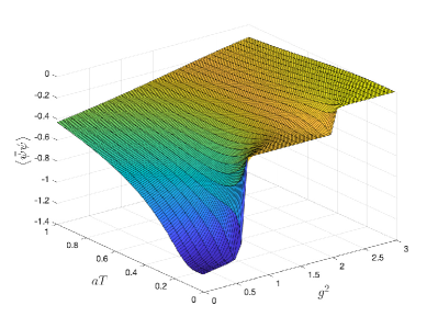
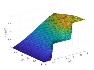
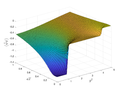
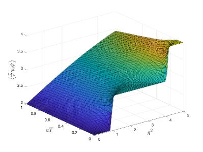
Figure 1: $\langle\bar{\psi}\psi\rangle$ (the left panels) and $\langle\bar{\psi}\gamma^{0}\psi\rangle$ (the right panels) as functions of $T$ and $g^{2}$ calculated by using exact diagonalization. The panels in the first row correspond to $H_{E}$, and the ones in the second row correspond to $H_{M}$, respectively.

Since $N=4$, it is also possible to perform exact diagonalization to calculate $e^{-\beta H}$. To focus on the errors in QMETTS, the discritization errors are ignored. In other words, the observables $\langle\bar{\psi}\psi\rangle$ and $\langle\bar{\psi}\gamma^{0}\psi\rangle$ are calculated using the Hamiltonian in Eq. (25), so that the deviations between the QMETTS and the exact diagonalization is purely due to the errors in QMETTS. The result of $\langle\bar{\psi}\psi\rangle$ and $\langle\bar{\psi}\gamma^{0}\psi\rangle$ are shown in Fig. 1. It can be seen that, the chiral symmetry is broken at either high temperatures or weak couplings. At low temperatures, the dependence of chiral condensation on the coupling constant is manifest in the form of distinct plateaus, which correspond to different topological charges. The values of the topological charge are integers at low temperatures, therefore exhibiting a topological structure.

The goal of our study is to reproduce the above results using QMETTS. Since $N=4$ is small, we use a complete set of bases of the Hilbert space, $\Phi_{i}=|i\rangle$, for $0\leq i\leq 15$. The range of temperature is $0.1a^{-1}\leq T\leq 2a^{-1}$, in other words, $0.5\leq\beta\leq 10$ with $\Delta\beta=0.25$ and $K=20$, where $K=\beta_{max}/(2\Delta\beta)$ is defined in previous section. Therefore, the temperatures in consideration is $a^{-1}/\left(2k\Delta\beta\right)$ with $1\leq k\leq K$. The number of steps in Trotter decomposition is $t=10$. In the evaluation, only the $\hat{\sigma}_{j}$ terms in Eq. (17) with $|a_{j}|>0.001$ are kept. In the case of $H_{M}$, the values of the coupling constant are chosen as $g^{2}=0,0.2,0.4,\ldots,5.0$. In the case of $H_{E}$, the values of the coupling constant are chosen as $g^{2}=0,0.1,0.2,\ldots,3.0$.

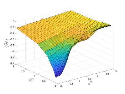
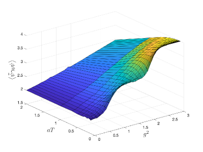
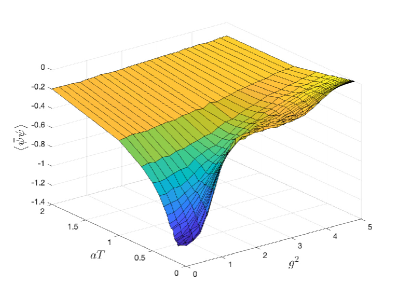
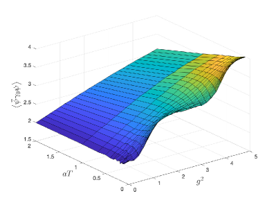
Figure 2: $\langle\bar{\psi}\psi\rangle$ (the left panels) and $\langle\bar{\psi}\gamma^{0}\psi\rangle$ (the right panels) as functions of $T$ and $g^{2}$ calculated by using QMETTS. The panels in the first row correspond to $H_{E}$, and the ones in the second row correspond to $H_{M}$, respectively.

The circuit is implemented using qiskit [74], and the results are obtained by using a simulator. The observables $\langle\bar{\psi}\psi\rangle$ and $\langle\bar{\psi}\gamma^{0}\psi\rangle$ at different temperatures and coupling constants are shown in Fig. 2. For simplicity, the parameters to calculate $a_{j}$ and $C(\beta)$ used in the evaluation are measured exactly which is only possible using a simulator, while $O_{i}$ in Eq. (24) are measured for $1024$ times. As can be seen from Figs. 1 and 2, the outcomes yielded by QMETTS are largely in alignment with those obtained through exact diagonalization. Among these results, the breaking and restoration of chiral symmetry, the plateaus in chiral condensation, and the behavior of topological charges are all consistent. In QMETTS, the jitter in the values is primarily attributable to the number of measurements. The edges of the plateaus at low temperatures are observed to be less sharp than in exact diagonalization, due to the fact that in QMETTS we only evolve up to $\beta=10$, in contrast to the exact diagonalization where $\beta=100$.

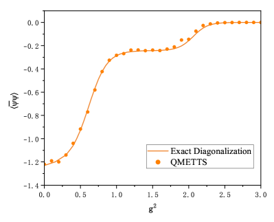
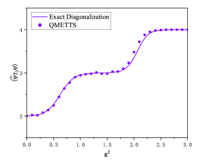
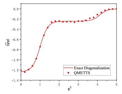
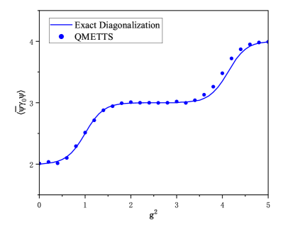
Figure 3: $\langle\bar{\psi}\psi\rangle$ (the left panels) and $\langle\bar{\psi}\gamma^{0}\psi\rangle$ (the right panels) as functions of $g^{2}$ at $T=0.1a^{-1}$. The solid curves are the results of exact diagonalization, while the dots are the results obtained by the QMETTS. The panels in the first row correspond to $H_{E}$, and the ones in the second row correspond to $H_{M}$, respectively.

In the QMETTS approach, the behaviors at large $\beta$ suffer from the accumulated errors from each $k\Delta\beta$ evolution. Whether the interesting behaviors at low temperatures can be reproduced is investigated. At $T=0.1a^{-1}$ (which is $T=10\;({\rm MeV})$), the observables are compared in Fig. 3. It can be seen that, even when $\beta=10$, the results from QMETTS are consistent with the results from exact diagonalization well.

In general, QMETTS reproduces results that are in accordance with those obtained through exact diagonalization. The outcomes demonstrate the breaking and restoration of chiral symmetry at different temperatures and different coupling constants. Furthermore, the integer values of the topological charges at low temperatures and the plateaus where the chiral symmetry varies with the coupling constant are also established.

V Summary

In this work, we use the QMETTS approach to study the thermal properties of a massive Thirring model, which is a soluble model for studying the interactions of fermions. The observables in interest are the chiral condensation which is related to the chiral phase transition, and the fermion number which corresponds to the topological charge in a sine-Gordon model dual to the massive Thirring model.

The results of the chiral condensation demonstrate that the chiral symmetry is broken at high temperatures, or at low temperatures and smaller coupling constants for the massive Thirring model. At low temperatures and larger coupling constants, the chiral symmetry is restored. This indicates the existence of a chiral phase transition in the massive Thirring model. Furthermore, it can be observed that at low temperatures, the fermion number of the massive Thirring model is an integer and exhibits quantized variation with the interaction. This suggests that the ground state of the corresponding sine-Gordon model is situated within a distinct topological sector, indicating a topological phase transition. Additionally, a quantized alteration in chiral condensation with fermion number is also observed at low temperatures.

A comparison of the results obtained from the QMETTS and exact diagonalization demonstrates that the utilisation of QMETTS is capable of reproducing the outcomes of the exact diagonalization. In particular, with regard to the low-temperature case, it is evident that the QMETTS error is not accumulated in line with the evolution of $\beta$. This indicates that the QMETTS remains a valid tool for the study of low-temperature systems, as well as physical systems exhibiting topological phase transitions. In light of these findings, this work offers a valuable reference point for future QMETTS or QITE-based studies. As quantum computing technology advances, it is plausible that one will be able to surmount the sign problem in lattice QCD with the aid of quantum computing.

Appendix A Details on the $\mathcal{O}(a)$ terms

The discretization of fermions into staggered fermions distributed over the two sites can result in the emergence of terms within a pair of sites. This leads to the presence of terms at every two sites. These spatially discontinuous terms can be reduced to spatially continuous terms, accompanied by an additional term of higher order in terms of the lattice spacing $a$. In this work, we choose to ignore these higher-order terms in order to maintain the spatial continuity of the Hamiltonian. With,

$$\begin{split}&\partial_{h}\chi(n)=\frac{1}{a}\left(\chi(n+2)-\chi(n)\right),\\ \end{split}$$ (28)

and Eqs. (2), (3) and (5), it can be verified,

$$\begin{split}&\sum_{h}\bar{\psi}(h)i\gamma_{1}\partial_{x}\psi(h)\\ &=-\frac{i}{a^{2}}\sum_{n}\left(\chi^{\dagger}(n)\chi(n+1)-\chi^{\dagger}(n+1)\chi(n)\right)\\ \end{split}$$ (29)

$$\begin{split}&a\sum_{h}\bar{\psi}(h)\psi(h)=\sum_{n}(-1)^{n}\chi^{\dagger}(n)\chi(n)\\ \end{split}$$ (30)

$$\begin{split}&a\sum_{h}\bar{\psi}(h)\gamma_{0}\psi(h)=\sum_{n}\chi^{\dagger}(n)\chi(n)\\ \end{split}$$ (31)

$$\begin{split}&a^{2}\sum_{h}(\bar{\psi}(h)\psi(h))^{2}=\\ &\sum_{n}\left\{(\chi^{\dagger}(n)\chi(n))^{2}-(\chi^{\dagger}(n)\chi(n))(\chi^{\dagger}(n+1)\chi(n+1))\right\}\\ &-a\sum_{even\;n}\left\{(\partial_{h}\chi^{\dagger}(n))\chi(n)\chi^{\dagger}(n+1)\chi(n+1)\right.\\ &\left.+\chi^{\dagger}(n+2)(\partial_{h}\chi(n))\chi^{\dagger}(n+1)\chi(n+1)\right\}\\ \end{split}$$ (32)

$$\begin{split}&a^{2}\sum_{h}(\bar{\psi}(h)\gamma_{0}\psi(h))^{2}=\\ &\sum_{n}\left((\chi^{\dagger}(n)\chi(n))^{2}+(\chi^{\dagger}(n)\chi(n))(\chi^{\dagger}(n+1)\chi(n+1))\right)\\ &+a\sum_{even\;n}\left\{(\partial_{h}\chi^{\dagger}(n))\chi(n)\chi^{\dagger}(n+1)\chi(n+1)\right.\\ &\left.+\chi^{\dagger}(n+2)(\partial_{h}\chi(n))\chi^{\dagger}(n+1)\chi(n+1)\right\}\\ \end{split}$$ (33)

$$\begin{split}&a^{2}\sum_{h}(\bar{\psi}(h)\gamma_{1}\psi(h))^{2}=\\ &\frac{1}{2}\sum_{n}\left(\chi^{\dagger}(n)\chi(n+1)+\chi^{\dagger}(n+1)\chi(n)\right)^{2}\\ &-\frac{a}{2}\sum_{even\;n}\left((\partial_{h}\chi^{\dagger}(n))\chi(n+1)\chi^{\dagger}(n)\chi(n+1)\right.\\ &\left.+\chi^{\dagger}(n+2)\chi(n+1)(\partial_{h}\chi^{\dagger}(n))\chi(n+1)\right.\\ &\left.+\chi^{\dagger}(n+1)(\partial_{h}\chi(n))\chi^{\dagger}(n)\chi(n+1)\right.\\ &\left.+\chi^{\dagger}(n+1)\chi(n+2)\chi^{\dagger}(n+1)(\partial_{h}\chi(n))\right)\\ &-\frac{a}{2}\sum_{even\;n}\left\{(\partial_{h}\chi^{\dagger}(n))\chi(n+1)\chi^{\dagger}(n)\chi(n+1)\right.\\ &\left.+\chi^{\dagger}(n+1)\chi(n+2)\chi^{\dagger}(n+1)(\partial_{h}\chi(n))\right.\\ &\left.+\chi^{\dagger}(n+1)(\partial_{h}\chi(n))\chi^{\dagger}(n)\chi(n+1)\right.\\ &\left.+\chi^{\dagger}(n+1)\chi(n+2)(\partial_{h}\chi^{\dagger}(n))\chi(n+1)\right\}\\ \end{split}$$ (34)

Ignoring the $\mathcal{O}(a)$ terms,

$$\begin{split}&a^{2}\sum_{h}(\bar{\psi}(h)\psi(h))^{2}=\\ &\sum_{n}(\chi^{\dagger}(n)\chi(n)\left(\chi^{\dagger}(n)\chi(n)-\chi^{\dagger}(n+1)\chi(n+1)\right)+\mathcal{O}(a)\\ \end{split}$$ (35)

$$\begin{split}&a^{2}\sum_{h}(\bar{\psi}(h)\gamma_{0}\psi(h))^{2}=\\ &\sum_{n}(\chi^{\dagger}(n)\chi(n)\left(\chi^{\dagger}(n)\chi(n)+\chi^{\dagger}(n+1)\chi(n+1)\right)+\mathcal{O}(a)\\ \end{split}$$ (36)

$$\begin{split}&a^{2}\sum_{h}(\bar{\psi}(h)\gamma_{1}\psi(h))^{2}=\\ &\frac{1}{2}\sum_{n}\left(\chi^{\dagger}(n)\chi(n+1)+\chi^{\dagger}(n+1)\chi(n)\right)^{2}+\mathcal{O}(a)\\ \end{split}$$ (37)

Then Eqs. (7-12) can be obtained by substituting $\chi$ with Eq. (6).

Appendix B Measurements to obtain $S$ and $b$

Since $|\phi(\beta)\rangle$ is a quantum state, the matrix elements of $S$ and $b$ can not be obtained classically. Therefore, the matrix elements of $S$ and $b$ should be obtained by measurement. Since the Hamiltonian can also been expanded using $H=\sum_{j}h_{j}\hat{\sigma}_{j}$, essentially, one needs a quick construction of $\hat{\sigma}_{j_{1}}\hat{\sigma}_{j_{2}}+\left(\hat{\sigma}_{j_{1}}\hat{\sigma}_{j_{2}}\right)^{T}$ and $-{\rm i}\left(\hat{\sigma}_{j_{1}}\hat{\sigma}_{j_{2}}-\hat{\sigma}_{j_{2}}\hat{\sigma}_{j_{1}}\right)$. Defining,

$$\begin{split}M_{a}=\begin{pmatrix}0&1&2&3\\ 1&0&3&2\\ 2&3&0&1\\ 3&2&1&0\end{pmatrix},\;\;&M_{b}=\begin{pmatrix}0&0&0&0\\ 0&0&1&1\\ 0&1&0&1\\ 0&1&1&0\end{pmatrix},\\ M_{c}=\begin{pmatrix}0&0&0&0\\ 0&0&1&0\\ 0&0&0&1\\ 0&1&0&0\end{pmatrix},\;\;&M_{d}=\begin{pmatrix}0&0&1&0\\ 0&0&0&1\\ 1&0&0&0\\ 0&1&0&0\end{pmatrix}.\\ \end{split}$$ (38)

Denoting the separate indices as $x,y$ for $j_{1}$ and $j_{2}$, respectively, i.e., $j_{1}=(x_{1},x_{2},\ldots)$ and $j_{2}=(y_{1},y_{2},\ldots)$, it can be verified,

$$\begin{split}&\hat{\sigma}_{j_{1}}\hat{\sigma}_{j_{2}}+\left(\hat{\sigma}_{j_{1}}\hat{\sigma}_{j_{2}}\right)^{T}=(-1)^{\sum_{i_{1}}\left(M_{c}^{T}\right)^{x_{i_{1}},y_{i_{1}}}}{\rm i}^{\sum_{i_{2}}M_{b}^{x_{i_{2}},y_{i_{2}}}}\\ &\times\left(1+(-1)^{\sum_{i_{3}}M_{d}^{x_{i_{3}},y_{i_{3}}}}\right)\prod_{l}\sigma^{M_{a}^{x_{l},y_{l}}}(l),\end{split}$$ (39)

and,

$$\begin{split}&-{\rm i}\left(\hat{\sigma}_{j_{1}}\hat{\sigma}_{j_{2}}-\hat{\sigma}_{j_{2}}\hat{\sigma}_{j_{1}}\right)=(-1)^{\sum_{i_{1}}M_{c}^{x_{i_{1}},y_{i_{1}}}}{\rm i}^{\left(1+\sum_{i_{2}}M_{b}^{x_{i_{2}},y_{i_{2}}}\right)}\\ &\times\left(1-(-1)^{\sum_{i_{3}}M_{b}^{x_{i_{3}},y_{i_{3}}}}\right)\prod_{l}\sigma^{M_{a}^{x_{l},y_{l}}}(l),\end{split}$$ (40)

where $M^{x,y}$ is the matrix element of $M$ at index $(x,y)$. $S+S^{T}$ in Eq. (18) can be obtained directly using Eq. (39). For the components of $b$ in Eq. (19), $b_{j}=\sum_{j^{\prime}}h_{j^{\prime}}\left\langle\phi|-{\rm i}\left(\hat{\sigma}_{j}\hat{\sigma}_{j^{\prime}}-\hat{\sigma}_{j^{\prime}}\hat{\sigma}_{j}\right)|\phi\right\rangle/\sqrt{C(\Delta\beta)}$, where $h_{j^{\prime}}$ are the coefficients in the expansion of Hamiltonian.

References

- Arute et al. [2019] F. Arute et al., Quantum supremacy using a programmable superconducting processor, Nature 574, 505 (2019), arXiv:1910.11333 [quant-ph] .
- Preskill [2018] J. Preskill, Quantum Computing in the NISQ era and beyond, Quantum 2, 79 (2018), arXiv:1801.00862 [quant-ph] .
- Chen et al. [2021] Z. Chen, K. J. Satzinger, J. Atalaya, A. N. Korotkov, A. Dunsworth, D. Sank, C. Quintana, M. McEwen, R. Barends, P. V. Klimov, S. Hong, C. Jones, A. Petukhov, D. Kafri, S. Demura, B. Burkett, C. Gidney, A. G. Fowler, A. Paler, H. Putterman, I. Aleiner, F. Arute, K. Arya, R. Babbush, J. C. Bardin, A. Bengtsson, A. Bourassa, M. Broughton, B. B. Buckley, D. A. Buell, N. Bushnell, B. Chiaro, R. Collins, W. Courtney, A. R. Derk, D. Eppens, C. Erickson, E. Farhi, B. Foxen, M. Giustina, A. Greene, J. A. Gross, M. P. Harrigan, S. D. Harrington, J. Hilton, A. Ho, T. Huang, W. J. Huggins, L. B. Ioffe, S. V. Isakov, E. Jeffrey, Z. Jiang, K. Kechedzhi, S. Kim, A. Kitaev, F. Kostritsa, D. Landhuis, P. Laptev, E. Lucero, O. Martin, J. R. McClean, T. McCourt, X. Mi, K. C. Miao, M. Mohseni, S. Montazeri, W. Mruczkiewicz, J. Mutus, O. Naaman, M. Neeley, C. Neill, M. Newman, M. Y. Niu, T. E. O’Brien, A. Opremcak, E. Ostby, B. Pató, N. Redd, P. Roushan, N. C. Rubin, V. Shvarts, D. Strain, M. Szalay, M. D. Trevithick, B. Villalonga, T. White, Z. J. Yao, P. Yeh, J. Yoo, A. Zalcman, H. Neven, S. Boixo, V. Smelyanskiy, Y. Chen, A. Megrant, and J. Kelly, Exponential suppression of bit or phase errors with cyclic error correction, Nature 595, 383 (2021), arXiv:2102.06132 .
- Fang et al. [2024] Y. Fang, C. Gao, Y.-Y. Li, J. Shu, Y. Wu, H. Xing, B. Xu, L. Xu, and C. Zhou, Quantum Frontiers in High Energy Physics (2024), arXiv:2411.11294 [hep-ph] .
- Scott et al. [2024] J. L. Scott, Z. Dong, T. Kim, K. Kong, and M. Park, Hybrid quantum-classical approach for combinatorial problems at hadron colliders (2024) arXiv:2410.22417 [hep-ph] .
- Roggero and Carlson [2019] A. Roggero and J. Carlson, Dynamic linear response quantum algorithm, Phys. Rev. C 100, 034610 (2019), arXiv:1804.01505 [quant-ph] .
- Roggero et al. [2020] A. Roggero, A. C. Y. Li, J. Carlson, R. Gupta, and G. N. Perdue, Quantum Computing for Neutrino-Nucleus Scattering, Phys. Rev. D 101, 074038 (2020), arXiv:1911.06368 [quant-ph] .
- Atas et al. [2021] Y. Y. Atas, J. Zhang, R. Lewis, A. Jahanpour, J. F. Haase, and C. A. Muschik, SU(2) hadrons on a quantum computer via a variational approach, Nature Commun. 12, 6499 (2021), arXiv:2102.08920 [quant-ph] .
- Lamm et al. [2020] H. Lamm, S. Lawrence, and Y. Yamauchi (NuQS), Parton physics on a quantum computer, Phys. Rev. Res. 2, 013272 (2020), arXiv:1908.10439 [hep-lat] .
- Li et al. [2022] T. Li, X. Guo, W. K. Lai, X. Liu, E. Wang, H. Xing, D.-B. Zhang, and S.-L. Zhu (QuNu), Partonic collinear structure by quantum computing, Phys. Rev. D 105, L111502 (2022), arXiv:2106.03865 [hep-ph] .
- Pérez-Salinas et al. [2021] A. Pérez-Salinas, J. Cruz-Martinez, A. A. Alhajri, and S. Carrazza, Determining the proton content with a quantum computer, Phys. Rev. D 103, 034027 (2021), arXiv:2011.13934 [hep-ph] .
- Jordan et al. [2014] S. P. Jordan, K. S. M. Lee, and J. Preskill, Quantum Computation of Scattering in Scalar Quantum Field Theories, Quant. Inf. Comput. 14, 1014 (2014), arXiv:1112.4833 [hep-th] .
- Mueller et al. [2020] N. Mueller, A. Tarasov, and R. Venugopalan, Deeply inelastic scattering structure functions on a hybrid quantum computer, Phys. Rev. D 102, 016007 (2020), arXiv:1908.07051 [hep-th] .
- Guan et al. [2021] W. Guan, G. Perdue, A. Pesah, M. Schuld, K. Terashi, S. Vallecorsa, and J.-R. Vlimant, Quantum Machine Learning in High Energy Physics, Mach. Learn. Sci. Tech. 2, 011003 (2021), arXiv:2005.08582 [quant-ph] .
- Wu et al. [2021a] S. L. Wu et al., Application of quantum machine learning using the quantum kernel algorithm on high energy physics analysis at the LHC, Phys. Rev. Res. 3, 033221 (2021a), arXiv:2104.05059 [quant-ph] .
- Zhang et al. [2024a] S. Zhang, Y.-C. Guo, and J.-C. Yang, Optimize the event selection strategy to study the anomalous quartic gauge couplings at muon colliders using the support vector machine and quantum support vector machine, Eur. Phys. J. C 84, 833 (2024a), arXiv:2311.15280 [hep-ph] .
- Zhang et al. [2024b] S. Zhang, K.-X. Chen, and J.-C. Yang, Detect anomalous quartic gauge couplings at muon colliders with quantum kernel k-means (2024) arXiv:2409.07010 [hep-ph] .
- Zhu et al. [2024] Y. Zhu, W. Zhuang, C. Qian, Y. Ma, D. E. Liu, M. Ruan, and C. Zhou, A Novel Quantum Realization of Jet Clustering in High-Energy Physics Experiments (2024) arXiv:2407.09056 [quant-ph] .
- Fadol et al. [2024] A. Fadol, Q. Sha, Y. Fang, Z. Li, S. Qian, Y. Xiao, Y. Zhang, and C. Zhou, Application of quantum machine learning in a Higgs physics study at the CEPC, Int. J. Mod. Phys. A 39, 2450007 (2024), arXiv:2209.12788 [hep-ex] .
- Wu et al. [2021b] S. L. Wu et al., Application of quantum machine learning using the quantum variational classifier method to high energy physics analysis at the LHC on IBM quantum computer simulator and hardware with 10 qubits, J. Phys. G 48, 125003 (2021b), arXiv:2012.11560 [quant-ph] .
- Terashi et al. [2021] K. Terashi, M. Kaneda, T. Kishimoto, M. Saito, R. Sawada, and J. Tanaka, Event Classification with Quantum Machine Learning in High-Energy Physics, Comput. Softw. Big Sci. 5, 2 (2021), arXiv:2002.09935 [physics.comp-ph] .
- Yang et al. [2024a] J.-C. Yang, S. Zhang, and C.-X. Yue, A novel quantum machine learning classifier to search for new physics (2024) arXiv:2410.18847 [hep-ph] .
- Feynman [1982] R. P. Feynman, Simulating physics with computers, Int. J. Theor. Phys. 21, 467 (1982).
- Georgescu et al. [2014] I. M. Georgescu, S. Ashhab, and F. Nori, Quantum Simulation, Rev. Mod. Phys. 86, 153 (2014), arXiv:1308.6253 [quant-ph] .
- Bauer et al. [2023] C. W. Bauer et al., Quantum Simulation for High-Energy Physics, PRX Quantum 4, 027001 (2023), arXiv:2204.03381 [quant-ph] .
- Carena et al. [2022] M. Carena, H. Lamm, Y.-Y. Li, and W. Liu, Improved Hamiltonians for Quantum Simulations of Gauge Theories, Phys. Rev. Lett. 129, 051601 (2022), arXiv:2203.02823 [hep-lat] .
- Gustafson et al. [2022] E. J. Gustafson, H. Lamm, F. Lovelace, and D. Musk, Primitive quantum gates for an SU(2) discrete subgroup: Binary tetrahedral, Phys. Rev. D 106, 114501 (2022), arXiv:2208.12309 [quant-ph] .
- Lamm et al. [2024] H. Lamm, Y.-Y. Li, J. Shu, Y.-L. Wang, and B. Xu, Block encodings of discrete subgroups on a quantum computer, Phys. Rev. D 110, 054505 (2024), arXiv:2405.12890 [hep-lat] .
- Carena et al. [2024] M. Carena, H. Lamm, Y.-Y. Li, and W. Liu, Quantum error thresholds for gauge-redundant digitizations of lattice field theories, Phys. Rev. D 110, 054516 (2024), arXiv:2402.16780 [hep-lat] .
- Li et al. [2024] Y.-Y. Li, M. O. Sajid, and J. Unmuth-Yockey, Lattice holography on a quantum computer, Phys. Rev. D 110, 034507 (2024), arXiv:2312.10544 [hep-lat] .
- Cui et al. [2020] X. Cui, Y. Shi, and J.-C. Yang, Circuit-based digital adiabatic quantum simulation and pseudoquantum simulation as new approaches to lattice gauge theory, JHEP 08, 160, arXiv:1910.08020 [quant-ph] .
- Zou et al. [2021] Y.-T. Zou, Y.-J. Bo, and J.-C. Yang, Optimize quantum simulation using a force-gradient integrator, EPL 135, 10004 (2021), arXiv:2103.05876 [quant-ph] .
- Echevarria et al. [2021] M. G. Echevarria, I. L. Egusquiza, E. Rico, and G. Schnell, Quantum simulation of light-front parton correlators, Phys. Rev. D 104, 014512 (2021), arXiv:2011.01275 [quant-ph] .
- Motta et al. [2019] M. Motta, C. Sun, A. T. K. Tan, M. J. O. Rourke, E. Ye, A. J. Minnich, F. G. S. L. Brandão, and G. K.-L. Chan, Determining eigenstates and thermal states on a quantum computer using quantum imaginary time evolution, Nature Phys. 16, 205 (2019), arXiv:1901.07653 [quant-ph] .
- Czajka et al. [2022] A. M. Czajka, Z.-B. Kang, H. Ma, and F. Zhao, Quantum simulation of chiral phase transitions, JHEP 08, 209, arXiv:2112.03944 [hep-ph] .
- Hasenfratz and Karsch [1983] P. Hasenfratz and F. Karsch, Chemical Potential on the Lattice, Phys. Lett. B 125, 308 (1983).
- de Forcrand [2009] P. de Forcrand, Simulating QCD at finite density, PoS LAT2009, 010 (2009), arXiv:1005.0539 [hep-lat] .
- Gattringer and Langfeld [2016] C. Gattringer and K. Langfeld, Approaches to the sign problem in lattice field theory, Int. J. Mod. Phys. A 31, 1643007 (2016), arXiv:1603.09517 [hep-lat] .
- Fukushima and Sasaki [2013] K. Fukushima and C. Sasaki, The phase diagram of nuclear and quark matter at high baryon density, Prog. Part. Nucl. Phys. 72, 99 (2013), arXiv:1301.6377 [hep-ph] .
- Busza et al. [2018] W. Busza, K. Rajagopal, and W. van der Schee, Heavy Ion Collisions: The Big Picture, and the Big Questions, Ann. Rev. Nucl. Part. Sci. 68, 339 (2018), arXiv:1802.04801 [hep-ph] .
- Aggarwal et al. [2010] M. M. Aggarwal et al. (STAR), An Experimental Exploration of the QCD Phase Diagram: The Search for the Critical Point and the Onset of De-confinement (2010) arXiv:1007.2613 [nucl-ex] .
- Gupta et al. [2011] S. Gupta, X. Luo, B. Mohanty, H. G. Ritter, and N. Xu, Scale for the Phase Diagram of Quantum Chromodynamics, Science 332, 1525 (2011), arXiv:1105.3934 [hep-ph] .
- Andronic et al. [2018] A. Andronic, P. Braun-Munzinger, K. Redlich, and J. Stachel, Decoding the phase structure of QCD via particle production at high energy, Nature 561, 321 (2018), arXiv:1710.09425 [nucl-th] .
- Luo et al. [2020] X. Luo, S. Shi, N. Xu, and Y. Zhang, A Study of the Properties of the QCD Phase Diagram in High-Energy Nuclear Collisions, Particles 3, 278 (2020), arXiv:2004.00789 [nucl-ex] .
- Abdallah et al. [2021] M. Abdallah et al. (STAR), Cumulants and correlation functions of net-proton, proton, and antiproton multiplicity distributions in Au+Au collisions at energies available at the BNL Relativistic Heavy Ion Collider, Phys. Rev. C 104, 024902 (2021), arXiv:2101.12413 [nucl-ex] .
- Stephans [2006] G. S. F. Stephans, critRHIC: The RHIC low energy program, J. Phys. G 32, S447 (2006), arXiv:nucl-ex/0607030 .
- Antoniou et al. [2006] N. Antoniou et al. (NA49-future), Study of hadron production in hadron nucleus and nucleus nucleus collisions at the CERN SPS (2006).
- Gazdzicki [2009] M. Gazdzicki (NA61/SHINE), Ion Program of Na61/Shine at the CERN SPS, J. Phys. G 36, 064039 (2009), arXiv:0812.4415 [nucl-ex] .
- Luo and Xu [2017] X. Luo and N. Xu, Search for the QCD Critical Point with Fluctuations of Conserved Quantities in Relativistic Heavy-Ion Collisions at RHIC : An Overview, Nucl. Sci. Tech. 28, 112 (2017), arXiv:1701.02105 [nucl-ex] .
- Stephanov [2004] M. A. Stephanov, QCD Phase Diagram and the Critical Point, Prog. Theor. Phys. Suppl. 153, 139 (2004), arXiv:hep-ph/0402115 .
- Fodor and Katz [2004] Z. Fodor and S. D. Katz, Critical point of QCD at finite T and mu, lattice results for physical quark masses, JHEP 04, 050, arXiv:hep-lat/0402006 .
- Gavai and Gupta [2005] R. V. Gavai and S. Gupta, The Critical end point of QCD, Phys. Rev. D 71, 114014 (2005), arXiv:hep-lat/0412035 .
- Yang et al. [2022] J.-C. Yang, X.-T. Chang, and J.-X. Chen, Study of the Roberge-Weiss phase caused by external uniform classical electric field using lattice QCD approach, JHEP 10, 053, arXiv:2207.11796 [hep-lat] .
- Yang and Huang [2023] J.-C. Yang and X.-G. Huang, QCD on Rotating Lattice with Staggered Fermions (2023), arXiv:2307.05755 [hep-lat] .
- Yang et al. [2024b] J.-C. Yang, X. Zhang, and J.-X. Chen, Study of the effects of external imaginary electric field and chiral chemical potential on quark matter, Eur. Phys. J. C 84, 746 (2024b), arXiv:2309.09281 [hep-lat] .
- Thirring [1958] W. E. Thirring, A Soluble relativistic field theory?, Annals Phys. 3, 91 (1958).
- Sachs and Wipf [1996] I. Sachs and A. Wipf, Generalized Thirring models, Annals Phys. 249, 380 (1996), arXiv:hep-th/9508142 .
- Mishra et al. [2020] C. Mishra, S. Thompson, R. Pooser, and G. Siopsis, Quantum computation of an interacting fermionic model, Quantum Sci. Technol. 5, 035010 (2020), arXiv:1912.07767 [quant-ph] .
- Hagen [1967] C. R. Hagen, New solutions of the thirring model, Nuovo Cimento B (1965-1970) 51, 169 (1967).
- Korepin et al. [1993] V. E. Korepin, N. M. Bogoliubov, and A. G. Izergin, Quantum Inverse Scattering Method and Correlation Functions, Cambridge Monographs on Mathematical Physics (Cambridge University Press, 1993).
- Alvarez-Estrada and Gomez Nicola [1998] R. F. Alvarez-Estrada and A. Gomez Nicola, The Schwinger and Thirring models at finite chemical potential and temperature, Phys. Rev. D 57, 3618 (1998), arXiv:hep-th/9710227 .
- Pinto Barros et al. [2019] J. C. Pinto Barros, M. Dalmonte, and A. Trombettoni, String tension and robustness of confinement properties in the Schwinger-Thirring model, Phys. Rev. D 100, 036009 (2019), arXiv:1808.00444 [hep-th] .
- Coleman [1975] S. R. Coleman, The Quantum Sine-Gordon Equation as the Massive Thirring Model, Phys. Rev. D 11, 2088 (1975).
- Bañuls et al. [2018] M. C. Bañuls, K. Cichy, Y.-J. Kao, C. J. D. Lin, Y.-P. Lin, and D. T.-L. Tan, Tensor Network study of the (1+1)-dimensional Thirring Model, EPJ Web Conf. 175, 11017 (2018), arXiv:1710.09993 [hep-lat] .
- Gross and Neveu [1974] D. J. Gross and A. Neveu, Dynamical Symmetry Breaking in Asymptotically Free Field Theories, Phys. Rev. D 10, 3235 (1974).
- Chen et al. [2010] X. Chen, Z. C. Gu, and X. G. Wen, Local unitary transformation, long-range quantum entanglement, wave function renormalization, and topological order, Phys. Rev. B 82, 155138 (2010), arXiv:1004.3835 [cond-mat.str-el] .
- Kogut and Susskind [1975] J. B. Kogut and L. Susskind, Hamiltonian Formulation of Wilson’s Lattice Gauge Theories, Phys. Rev. D 11, 395 (1975).
- Kluberg-Stern et al. [1983] H. Kluberg-Stern, A. Morel, O. Napoly, and B. Petersson, Flavors of Lagrangian Susskind Fermions, Nucl. Phys. B 220, 447 (1983).
- Morel and Rodrigues [1984] A. Morel and J. P. Rodrigues, How to Extract QCD Baryons From a Lattice Theory With Staggered Fermions, Nucl. Phys. B 247, 44 (1984).
- Jordan and Wigner [1928] P. Jordan and E. Wigner, Über das Paulische Äquivalenzverbot, Zeitschrift fur Physik 47, 631 (1928).
- Delepine et al. [1998] D. Delepine, R. Gonzalez Felipe, and J. Weyers, Equivalence of the sine-Gordon and massive Thirring models at finite temperature, Phys. Lett. B 419, 296 (1998), arXiv:hep-th/9709039 .
- Shen et al. [2024] Y. Shen, K. Klymko, E. Rabani, N. M. Tubman, D. Camps, R. Van Beeumen, and M. Lindsey, Simple Diagonal Designs with Reconfigurable Real-Time Circuits (2024), arXiv:2401.04176 [quant-ph] .
- Lloyd [1996] S. Lloyd, Universal Quantum Simulators, Science 273, 1073 (1996).
- Javadi-Abhari et al. [2024] A. Javadi-Abhari, M. Treinish, K. Krsulich, C. J. Wood, J. Lishman, J. Gacon, S. Martiel, P. D. Nation, L. S. Bishop, A. W. Cross, B. R. Johnson, and J. M. Gambetta, Quantum computing with Qiskit (2024), arXiv:2405.08810 [quant-ph] .