Combinatorial Rising Bandit

Abstract

Combinatorial online learning is a fundamental task to decide the optimal combination of base arms in sequential interactions with systems providing uncertain rewards, which is applicable to diverse domains such as robotics, social advertising, network routing and recommendation systems. In real-world scenarios, we often observe rising rewards, where the selection of a base arm not only provides an instantaneous reward but also contributes to the enhancement of future rewards, e.g., robots enhancing proficiency through practice and social influence strengthening in the history of successful recommendations. To address this, we introduce the problem of combinatorial rising bandit to minimize policy regret and propose a provably efficient algorithm, called Combinatorial Rising Upper Confidence Bound (CRUCB), of which regret upper bound is close to a regret lower bound. To the best of our knowledge, previous studies do not provide a sub-linear regret lower bound, making it impossible to assess the efficiency of their algorithms. However, we provide the sub-linear regret lower bound for combinatorial rising bandit and show that CRUCB is provably efficient by showing that the regret upper bound is close to the regret lower bound. In addition, we empirically demonstrate the effectiveness and superiority of CRUCB not only in synthetic environments but also in realistic applications of deep reinforcement learning.

1 Introduction

Combinatorial online learning addresses a fundamental problem in sequential decision-making systems where the learner aims to find an optimal combination of sub-actions (or base arms) to maximize rewards while balancing the trade-off between exploring under-explored actions and exploiting current experiences on systems. This problem has been extensively studied in various frameworks, including combinatorial multi-armed bandit and Markov decision process, as well as a wide range of domains such as robotics (Kober, Bagnell, and Peters 2013), social advertising (Wen et al. 2017), automatic machine learning (Li et al. 2018), network routing (Talebi et al. 2017), and recommendation systems (Li et al. 2016).

However, the previous studies of combinatorial online learning have often overlooked the presence of rising nature in practice, where selecting a base arm not only yields an immediate outcome but also enhances future outcomes. For instance, in deep reinforcement learning, an agent improves its skills through repeated practice (Vezhnevets et al. 2017). In online social marketing, the influence in a social relationship strengthens over the history of interactions or recommendations (Wu et al. 2020).

In this paper, we study a regret minimization problem in a combinatorial rising bandit, where the agent selects a set of base arms (referred to as a super arm) while the outcome of each base arm rises over trials. This is challenging mainly because just characterizing the optimal policy is intractable in general. Characterization of the optimal policy is crucial as it provides important intuition for designing algorithm. We hence establish a theoretical framework based on canonical assumptions: additive reward of super arm (Assumption 1 (Chen, Du, and Kuroki 2020; Nourani-Koliji, Ghoorchian, and Maghsudi 2022) and concave rising outcome of base arm 2) (Heidari, Kearns, and Roth 2016; Metelli et al. 2022). This enables the characterization of the optimal policy and provides the analytical tractability of regret analysis.

For the regret minimization in the combinatorial rising bandit, we propose a simple and provably efficient algorithm called Combinatorial Rising UCB (CRUCB). In each round, CRUCB computes the recent mean and slope of each base arm’s outcome and optimistically estimates the future potential $\acute{\mu}$ of each base arm at a certain time being aware of both the rising and random outcome. Then, it selects a super arm combinatorially maximizing the future potential. For CRUCB, we establish an upper bound of regret that can be parameterized by $c$ governing the curvature of rising outcomes. A larger $c$ leads to the rising outcome reaching the maximum value more quickly. We also provide a regret lower bound that has a small gap to the upper bound for different $c$, i.e., CRUCB is provably efficient while it requires no knowledge on $c$. To the best of our knowledge, it is first to provide a sub-linear regret lower bound for online learning framework with rising nature.

In addition to the regret analysis of CRUCB, we also demonstrate the superiority of CRUCB compared to a set of baselines in various experiments. To be specific, our experiments include not only synthetic environments, emulating resource allocation (Chen et al. 2020) and network routing (Talebi et al. 2017), but also standard scenarios of deep reinforcement learning (RL), training a neural agent for navigation tasks. We note that in the deep RL experiment, the base arm outcome is not concave, but CRUCB outperforms the other baselines. This suggests a broader applicability of CRUCB in practice.

Our main contributions are summarized as follows:

• We introduce the combinatorial rising bandit, which is inadequately addressed by existing rising bandit and non-stationary combinatorial bandit algorithms.

• We propose CRUCB, a simple and provably efficient algorithm for the combinatorial rising bandit.

• We analyze CRUCB’s regret upper bound parameterized by curvature $c$ and show that it has small gap to the regret lower bound.

• We conduct extensive experiments in both synthetic environments and deep reinforcement learning settings to demonstrate CRUCB’s practical applicability and effectiveness.

2 Related works

2.1 Combinatorial bandit

Combinatorial bandit has been extensively studied due to its relevance in various applications such as online advertising, recommendation systems, and resource allocation. Due to the importance and extensibility of combinatorial bandit, various variations of combinatorial bandit have been studied (Kveton et al. 2015a; Wang, Chen, and Vojnović 2023). Combinatorial bandit can be categorized based on the characteristics of the feedback: semi-bandit feedback and full-bandit feedback. In the semi-bandit feedback setting, the feedback includes all outcomes of base arms in the selected super arm. Chen, Wang, and Yuan (2013); Kveton et al. (2015b); Wang and Chen (2018) considered semi-bandit feedback. In the full-bandit feedback setting, the feedback only includes the final reward but no outcomes of the base arms, which is considered in (Combes et al. 2015). In our problem setting, we consider the semi-bandit feedback setting. Especially, Chen et al. (2021) proposes the SW-CUCB for non-stationary combinatorial bandit under the semi-bandit feedback setting, which is closest to our work in combinatorial bandit works. However, We emphasize that there have not been any researches considering rising bandit in combinatorial setting. Rising bandit is distinct from the general non-stationary setting, which will be explained in detail in the following section.

2.2 Non-stationary bandit

Non-stationary bandit has been extensively studied because it is well-suited to model real-world scenarios(Garivier and Moulines 2011; Besbes, Gur, and Zeevi 2014; Wei and Srivatsva 2018; Cao et al. 2019; Trovo et al. 2020). These common non-stationary settings considered in these previous studies are also called as the restless bandit, since reward shift can occur restlessly, which means that reward shift occurs regardless of whether the arms are pulled. In contrast to this, in rested bandit, which has been introduced in (Tekin and Liu 2012), the reward of each arm changes depending on the number of pulls. Research on rested rising bandit has been conducted by (Heidari, Kearns, and Roth 2016; Metelli et al. 2022). We consider a rested rising bandit setting, which means that the reward of each arm changes and is non-decreasing over the number of pulls. The rested rising bandit has been considered in many papers. Xia et al. (2024) applied the rested rising bandit to model selection for LLM. Metelli et al. (2022) proposes R-ed-UCB to handle the rested rising bandit setting. However, these previous researches do not consider the combinatorial nature.

3 Problem formulation

A combinatorial rising bandit problem consists of $K$ base arms and a set $\mathcal{S}\subset 2^{K}$, where a super arm $S\in\mathcal{S}$ is a combination of base arms. Each base arm $i$ is associated with a rising function $\mu_{i}:[T]\mapsto[0,1]$ such that

$$\gamma_{i}(n):=\mu_{i}(n+1)-\mu_{i}(n)\geq 0\;.$$ (1)

We note that we bound $\mu_{i}(n)\in[0,1]$ without loss of generality. If a super arm $S\in\mathcal{S}$ is selected at time $t\in[T]$, then each base arm $i\in S$ produces the outcome $X_{i}(t)$ drawn from a $\sigma^{2}$-subgaussian distribution of mean $\mu_{i}(N_{i,t})$ for known $\sigma^{2}$ where $N_{i,t}$ is the number of playing base arm $i$ up to time $t$, i.e., the combinatorial rising bandit is parameterized by $\bm{\mu}:=(\mu_{i}(n):i\in[K],n\in[T])$. Let $O_{t}:=\{(i,X_{i}(t)):i\in S_{t}\}$ denote the outcomes at time $t$. We consider a canonical setting of semi-bandit feedback. At time $t\in[T]$, a policy $\pi$ selects $S_{t}$ based on the history $\mathcal{F}_{t-1}:=\{(S_{t^{\prime}},O_{t^{\prime}}):{t^{\prime}}\in[t-1]\}$. We assume an additive reward for selecting super arm $S$ (Chen, Du, and Kuroki 2020; Nourani-Koliji, Ghoorchian, and Maghsudi 2022):

Assumption 1.

Selecting super arm $S$ at time $t$ provides the sum of the outcomes of the selected base arms:

$$X_{S}(t)=\sum_{i\in S}X_{i}(t)\;.$$ (2)

In addition, we assume that $\mu_{i}(n)$ is concave. More formally,

Assumption 2.

For each $i\in[K]$ and $n\in[T-1]$,

$$\gamma_{i}(n+1)\leq\gamma_{i}(n)\;.$$ (3)

In (3), the reward gain is diminishing over $n$ and thus it follows that $\mu_{i}(n)$ is concave. We note that the concavity assumption is plausible in practice. Indeed, it is employed in previous studies as well (Heidari, Kearns, and Roth 2016; Metelli et al. 2022).

3.1 Regret minimization

The objective of the agent is to minimize regret. The optimal policy $\pi^{*}$ is defined as the policy maximizes the expected cumulative reward:

$$\pi^{*}:=\operatorname*{arg\,max}_{\pi}\mathbb{E}_{S_{t}\sim\pi}\Bigg{[}\sum_{t\in[T]}\!X_{S_{t}}\!(t)\Bigg{]}\;.$$ (4)

For a given policy $\pi$, the regret is defined as the difference between the expected cumulative reward of $\pi^{*}$ and that of $\pi$, which is defined as follows:

$$R_{\bm{\mu}}(\pi,T)$$

$$\coloneqq{\color[rgb]{1,.5,0}\underbrace{\mathbb{E}_{S_{t}\sim\pi^{*}}\!\Bigg{[}\!\sum_{t\in[T]}\!X_{S_{t}}\!(t)\!\Bigg{]}}_{\text{(reward of the optimal policy)}}}\!-{\color[rgb]{0,1,1}\underbrace{\mathbb{E}_{S_{t}\sim\pi}\!\Bigg{[}\!\sum_{t\in[T]}\!X_{S_{t}}\!(t)\!\Bigg{]}}_{\text{(reward of the given policy)}}}\;.$$ (5)

We note that this regret definition is called policy regret (Heidari, Kearns, and Roth 2016; Arora, Dekel, and Tewari 2012). We remark that policy regret is different from weak regret or dynamic regret, which are mainly used in the oblivious adversarial bandit (Auer et al. 2002; Wei and Luo 2018) and the non-stationary bandit (Besbes, Gur, and Zeevi 2014; Trovo et al. 2020; Cao et al. 2019). In the weak regret and the dynamic regret, the optimal policy is determined based on the history $\mathcal{F}_{t-1}$ generated by the given policy. These definitions are reasonable when the reward shift and the history $\mathcal{F}_{t-1}$ are independent. However, in the combinatorial rising bandit, the reward shift depends on the history $\mathcal{F}_{t-1}$, which means that a different history might lead to higher reward. While in policy regret, the optimal policy is determined independently of the history generated by the given policy, which is proper for the combinatorial rising bandit.

3.2 Characterization of the optimal policy

We show that the oracle constant policy, which involves pulling the optimal super arm continuously, is optimal in the combinatorial rising bandit under Assumption 1.

Theorem 1.

Define $S^{{\dagger}}(\bm{\mu},T)$ as follows:

$$S^{{\dagger}}(\bm{\mu},T):=\operatorname*{arg\,max}_{S\in\mathcal{S}}\mathbb{E}\left[\sum_{t\in[T]}X_{S}(t)\right]\;.$$ (6)

Under Assumption 1, the oracle constant policy, which involves pulling $S^{{\dagger}}(\bm{\mu},T)$ at every time step, is the optimal policy in the combinatorial rising bandit.

Theorem 1 characterizes the optimal policy in the combinatorial rising bandit. Characterizing the optimal policy in an unconstrained combinatorial bandit is intractable in general. However, in the combinatorial rising bandit, selecting one optimal super arm continuously is guaranteed to be the optimal policy under Assumption 1. We note that in the asymptotic regime, the optimal policy is to select the super arm with the highest future potential, which is the core intuition of our algorithm. A detailed proof is given in Appendix A.1.

Also, we emphasize the importance of Assumption 1. Without Assumption 1, the oracle constant policy is not guaranteed to be the optimal policy.

Theorem 2.

Without Assumption 1, the oracle constant policy is not guaranteed to be the optimal policy in the combinatorial rising bandit.

Proof.

It suffices to show that there exists a combinatorial rising bandit problem instance such that the oracle constant policy is not the optimal policy: the K-max bandit problem (Chen et al. 2016). In the K-max bandit problem, the reward of a super arm is defined as follows:

$$X_{S}(t):=\max_{i\in S}(X_{i}(t))$$ (7)

Note that (7) does not satisfy the Assumption 1. Consider $\bm{\mu}$ such that:

$$\mu_{1}(n)=\begin{cases}\frac{10}{T}n&n<\frac{T}{10}\\ 1&n\geq\frac{T}{10}\end{cases}\;;$$ (8)

$$\mu_{2}(n)=\begin{cases}0.1&n=1\\ 0.9&n>1\end{cases}\;;$$ (9)

$$\mu_{3}(n)=0.5\;.$$ (10)

Let $\mathcal{S}=\left\{(1,2),(1,3),(2,3)\right\}$ and $T\gg 100$. The oracle constant policy is playing the super arm $(1,2)$ continuously. When we play the super arm $(1,2)$ continuously, we get $0.1$ once, $0.9$ for $(\frac{9T}{100}-1)$ times, about $0.95$ for $(\frac{T}{100})$ times, and $1$ for $\frac{9T}{10}$ times. However, if we play the super arm $(2,3)$ once and then play the super arm $(1,2)$ for the remaining time, we get $0.5$ once and $0.9$ for $\frac{9T}{100}$ times, about $0.95$ for $(\frac{T}{100})$ times, and $1$ for $(\frac{9T}{10}-1)$ times. This receives $0.3$ more reward than playing the super arm $(1,2)$ continuously, which means that the oracle constant policy is not optimal. ∎

4 Proposed method: CRUCB

Algorithm 1 ​Combinatorial Rising UCB​​ (CRUCB)​​

 Input $N_{i,0}\leftarrow 0$ for all $i\in[K]$, Sliding window parameter $\varepsilon$.

 Initialize Play arbitrary super arm including base arm $i$ two times for each $i\in[K]$.

 for $t\in(1,\dots,T)$ do

  For each base arm $i$, set $\acute{\mu}_{i}(t)=\hat{\mu}_{i}(t)+\beta_{i}(t)$.

  $S_{t}\leftarrow$ Solver($\acute{\mu}_{1}(t),\acute{\mu}_{2}(t),\cdots,\acute{\mu}_{K}(t)$).

  Play $S_{t}$ and observe reward $X_{S_{t}}(t)$.

  Update $\hat{\mu}_{i}(t)$ and $N_{i,t}$.

 end for

In this section, we propose CRUCB for combinatorial rising bandit. CRUCB operates through two distinct stages: ($i$) estimating future potential of each base arm, and ($ii$) employing the Solver to find the optimal super arm based on the base arm estimations. CRUCB is described in Algorithm 1.

Estimation

CRUCB estimates the future potential of each base arm using the reward estimator from the non-combinatorial rising bandit algorithm (Metelli et al. 2022). Specifically, the future potential of a base arm $i$ at time step $t$ is denoted as $\acute{\mu}_{i}(t)$ and defined as follows:

$$\hat{\mu}_{i}(t) :=\frac{1}{h_{i}}\sum_{l=N_{i,t-1}-h_{i}+1}^{N_{i,t-1}}\Bigg{(}\color[rgb]{1,.5,0}\underbrace{X_{i}(l)}_{\text{(to estimate recent mean)}}$$

$$\quad+(t-l)\color[rgb]{0,1,1}\underbrace{\frac{X_{i}(l)-X_{i}(l-h_{i})}{h_{i}}}_{\text{(to estimate recent slope)}}\color[rgb]{0,0,0}\Bigg{)}\;;$$ (11)

$$\beta_{i}(t) :=\underbrace{\sigma\left(t-N_{i,t-1}+h_{i}-1\right)\sqrt{\frac{10\log t^{3}}{h_{i}^{3}}}}_{\text{(confidence interval)}}\;;$$ (12)

$$\acute{\mu}_{i}(t) :=\hat{\mu}_{i}(t)+\beta_{i}(t)\;,$$ (13)

where $\sigma$ represents the standard deviation and $h_{i}$ denotes the size of the sliding window.

$\acute{\mu}_{i}(t)$ is estimating $\mu_{i}(t)$, which is the expectation of instantaneous reward of arm $i$ when it is pulled $t$-th times. The intuition behind $\acute{\mu_{i}}(t)$ is that the optimal super arm is likely to have the highest reward after being played sufficiently many times. To estimate future potential $\mu_{i}(t)$, CRUCB estimates the slope of the reward with finite difference method. This estimated reward is guaranteed to be optimistic due to the concavity assumption (Assumption 2).

Solver

After estimating the reward of each base arm, CRUCB employ the Solver that utilizes a task-specific greedy algorithm, such as Dijkstra’s algorithm for online shortest path problems. Following the Solver’s decision, CRUCB selects the super arm $S_{t}$ and update every base arm within the selected super arm $S_{t}$ based received feedback.

5 Regret analysis

In this section, we provide a regret analysis under Assumptions 1 and 2. For simplicity, we omit mentioning them in each theorem presented here.

5.1 Regret upper bound of CRUCB

We provide the regret upper bound analysis of CRUCB. To characterize the rising bandit problem instance, we borrow the cumulative increment (Metelli et al. 2022):

$$\Upsilon_{\bm{\mu}}(M,q):=\sum_{l=1}^{M-1}\max_{i\in[K]}\{\gamma_{i}(l)^{q}\}\;.$$ (14)

The cumulative increment reflects the difficulty of a problem instance. If $\Upsilon_{\bm{\mu}}(M,q)$ is close to 0, the reward function does not change substantially, indicating that the problem instance is similar to a stationary-bandit and therefore easier to solve. Conversely, the larger $\Upsilon_{\bm{\mu}}(M,q)$ is, the more the reward function changes, implying that the problem instance is more challenging to solve. We note that $\Upsilon_{\bm{\mu}}(M,q)$ corresponds to the variation budget (Besbes, Gur, and Zeevi 2014), which is widely used to quantify difficulty in non-stationary bandit problems.

The regret upper bound of CRUCB is given as follows:

Theorem 3.

Let $\pi_{\varepsilon}$ be CRUCB with $h_{i}=\varepsilon N_{i,t}$. For $T>0$, $q\in[0,1]$, and $\varepsilon\in(0,\frac{1}{2})$, we have the following regret upper bound:

$$\!\!\!R_{\bm{\mu}}(\pi_{\varepsilon},T) \leq\left(2+\frac{L\pi}{3}\right)K$$ (15)

$$+KT^{q}\left(\frac{1}{1-2\varepsilon}\right)\Upsilon_{\bm{\mu}}\left((1-2\varepsilon)\frac{LT}{K},q\right)$$ (16)

$$+O(T^{\frac{2}{3}}\log T^{\frac{1}{3}})\;,$$ (17)

where $L:=\max_{S\in\mathcal{S}}|S|$ is the maximal size of super arms.

We provide high-level comments for each term. (16) represents the regret due to rising property, which is related to the cumulative increment $\Upsilon_{\bm{\mu}}$. We remark that we can choose $q$ depending on problem instance $\bm{\mu}$ for optimization. (17) represents the uncertainty of reward.

A detailed proof can be found in Appendix A.2. We remark that if $\Upsilon_{\bm{\mu}}$ is small, then, the dominant term of regret is (17). More precisely, we discuss the condition of $\bm{\mu}$ to make regret upper bound sub-linear.

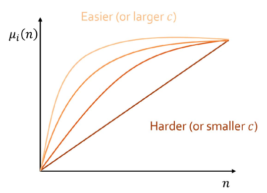
Figure 1: Reward function growth under $(n+1)^{-c}$ constraint. This figure illustrates the change of reward function when the constraint is given as $\gamma_{i}(n)\leq(n+1)^{-c}$. When $c$ is smaller, the more time steps are required to reach the maximum value, causing the algorithm to take more samples to determine whether each base arm has high potential. Conversely, when $c$ is larger, fewer time steps are needed to reach the maximum value, allowing the algorithm to make a quicker judgement about the potential of each base arm.

Corollary 1.

Assume $\bm{\mu}$ satisfies such that:

$$\gamma_{i}(n)\leq f(n),\quad\forall i\in[K],\forall n\in[T-1],$$ (18)

where $f$ is a non-increasing real-valued function. For $T\geq 0$ and, $q\in[0,1]$, and $\varepsilon\in(0,\frac{1}{2})$, $\pi_{\varepsilon}$ has following regret upper bound:

$$R_{\bm{\mu}}(\pi_{\varepsilon},T)$$

$$\!\leq\!O\!\left(\!\max\!\left(\!T^{\frac{2}{3}}\log KT^{\frac{1}{3}},KT^{q}\!\!\int_{1}^{(1-2\varepsilon)\frac{LT}{K}}\!\!f(n)^{q}dn\right)\right).$$ (19)

Under additional constraints (18), the regret upper bound becomes more explicit. When the integral of $f(n)$ is large, the cumulative increment is also large, leading to difficult problem. In such cases, the regret upper bound is dominated by (16), which can be linear regret. Conversely, when the integral of $f(n)$ is small, the cumulative increment is also small, leading to simpler problem. In such cases, the regret upper bound is dominated by (17), which implies sub-linear regret. When $f(n)=(n+1)^{-c}$, the relationship between reward function and constraint parameter $c$ is given in Figure 1.

We provide some interpretations of Corollary 1 for different choice of $f(n)$.

• When $f(n)=(n+1)^{-c}$ and $c>1$, we have:

  $$R_{\bm{\mu}}(\pi_{\varepsilon},T)\leq O\left(\max\left(T^{\frac{2}{3}}\log KT^{\frac{1}{3}},T^{\frac{1}{c}}\log\frac{LT}{K}\right)\right)\;.$$ (20)

• When $f(n)=(n+1)^{-c}$ and $c<1$, we have:

  $$R_{\bm{\mu}}(\pi_{\varepsilon},T)\leq O(LT)\;.$$ (21)

• When $f(n)=\exp(-n)$, we have:

  $$R_{\bm{\mu}}(\pi_{\varepsilon},T)\leq O(T^{\frac{2}{3}}\log KT^{\frac{1}{3}})\;.$$ (22)

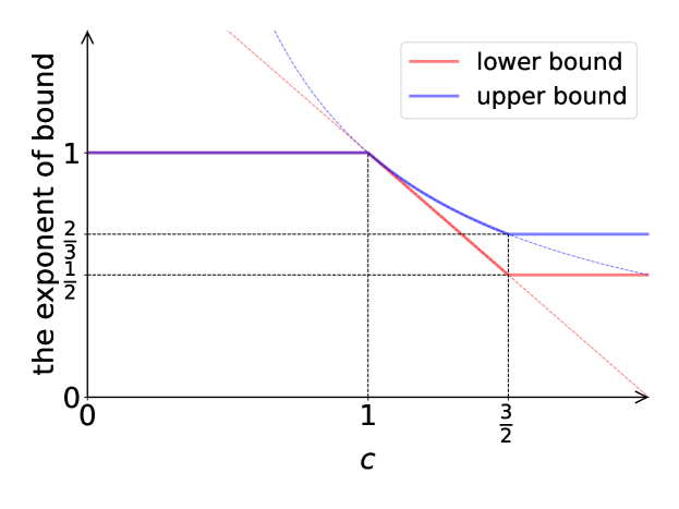
Figure 2: Regret bound gap. We compare the lower bound of the combinatorial rising bandit and the upper bound of CRUCB when $f(n)=(n+1)^{-c}$. The regret upper bound is $\tilde{O}\left(\min\left\{\max\left\{T^{\frac{2}{3}},T^{\frac{1}{c}}\right\},T\right\}\right)$, represented by the blue line. The regret lower bound is $\tilde{O}\left(\min\left\{\max\left\{T^{\frac{1}{2}},T^{2-c}\right\},T\right\}\right)$, depicted by the red line. When $c<1$, both the regret upper bound and the regret lower bound are $\tilde{O}(T)$, indicating that the problem nearly impossible to solve. When $c$ is in the range $[1,\frac{3}{2}]$, the regret upper bound is $\tilde{O}(T^{\frac{1}{c}})$ and the regret lower bound is $\tilde{O}(T^{2-c})$. When $c>\frac{3}{2}$, the regret upper bound is $\tilde{O}(T^{\frac{2}{3}})$ and the regret lower bound is $\tilde{O}(T^{\frac{1}{2}})$, indicating that when $c$ is large, the combinatorial rising bandit behaves similarly to combinatorial stationary bandit.

5.2 Regret lower bound

We show that the regret upper bound of our CRUCB nearly matches the lower bound of the combinatorial rising bandit. As mentioned in (21), the regret upper bound can be linear if a combinatorial rising bandit problem instance is too difficult, that is, the cumulative increment has large value. However, when the combinatorial rising bandit problem instance is too difficult, the worst case regret lower bound is also linear.

Theorem 4.

(Lower bound without constraints) Let $\mathcal{I}$ be the set of all available combinatorial rising bandit problem. For sufficiently large time $T$, any policy $\pi$ suffers regret:

$$\min_{\pi}\max_{\bm{\mu}\in\mathcal{I}}R_{\bm{\mu}}(\pi,T)\geq\frac{L}{32}T\;,$$ (23)

where $L$ is the maximal size of super arms.

Theorem 4 indicates that without any additional constraints, no algorithm can achieve sub-linear regret. A detailed proof is given in Appendix A.3. Conversely, as mentioned in (20), the regret upper bound can be sub-linear if the growth of every base arm is restricted.

Theorem 5.

(Lower bound with constraints) For an arbitrary constant $c>1$, define a subset of the combinatorial rising bandit problem with constraints $\mathcal{A}_{c}$ as follows:

$$\mathcal{A}_{c}:=\left\{\bm{\mu}:\gamma_{i}(n-1)\leq(n+1)^{-c}\quad i\in[K],n\in[T-1]\right\}\;,$$ (24)

For a sufficiently large $T$, any policy $\pi$ suffers regret:

$$\min_{\pi}\max_{\bm{\mu}\in\mathcal{A}_{c}}R_{\bm{\mu}}(\pi,T)\geq\Omega\left(\max\left\{L\sqrt{T},LT^{2-c}\right\}\right)\;,$$ (25)

where $L$ is the maximal size of super arms.

Theorem 5 implies that the regret lower bound of the combinatorial rising bandit decreases as the growth of reward is restricted. Intuitively, when the growth of reward is strongly restricted, the combinatorial rising bandit is similar to stationary bandit problem, which has $O(\sqrt{T})$ lower bound. A detailed proof is given in Appendix A.4.

Theorem 4 and Theorem 5 characterize the lower bound of combinatorial rising bandit. We highlight that CRUCB nearly matches this lower bound, which is shown in Figure 2. Figure 2 demonstrates the transition from linear to sub-linear worst regret, and how our CRUCB method nearly achieves the worst-case lower bound. It shows that when the lower bound is sub-linear, CRUCB also achieves the sub-linear upper bound and its gab is not very large.

Furthermore, we highlight that CRUCB is provably efficient since it requires no prior knowledge of such constraint, which highlights its robustness and practical applicability. This allows CRUCB to adapt to a wide range of scenarios, making it versatile and effective even in environments where the constraints are unknown or difficult to estimate. This will be further supported by experiments in the next section.

6 Experiments

In this section, we conduct experiments to compare CRUCB with existing state-of-the-art algorithms for rising bandit and non-stationary bandit across diverse combinatorial tasks. We evaluate CRUCB’s performance against baseline algorithms in both synthetic environments (Section 6.2) and realistic applications of deep reinforcement learning (Section 6.3).

6.1 Experimental setup

We introduce the baseline algorithms and the specific tasks used for evaluation. Detailed pseudocode and descriptions of the baselines are provided in Appendix C.

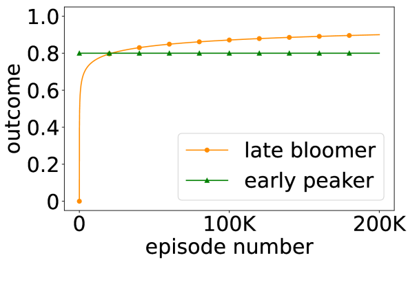
(a) rewards of each arm

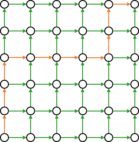
(b) Online shortest path

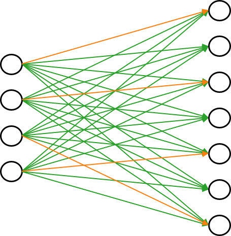
(c) Maximum weighted matching

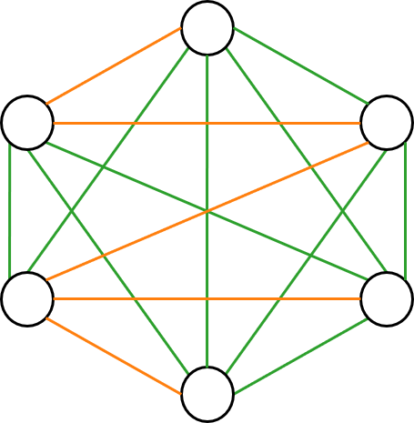
(d) Minimum spanning tree

Figure 3: Synthetic environments. We evaluate CRUCB and the baselines in the set of synthetic environments depicted above. (a) Outcome graphs illustrating two types of edges: a late bloomer with initially low but rising outcomes, and an early peaker with initially high but non-rising outcomes. Graph structures used in each task are shown in (b) Online shortest path, (c) Maximum weighted matching, and (d) Minimum spanning tree.

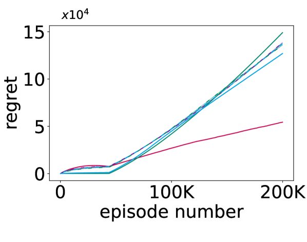
(a) Online shortest path

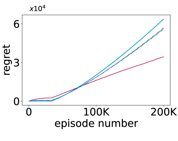
(b) Maximum weighted matching

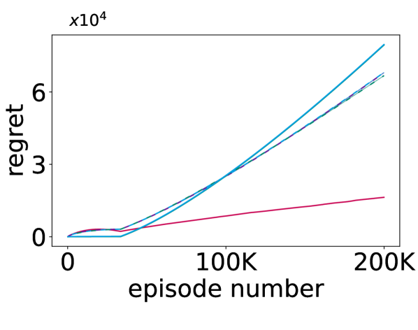
(c) Minimum spanning tree

Figure 4: Cumulative regret for each task in synthetic environments. We report the average cumulative regret as a line and the 99% confidence interval as a shaded region, based on 5 runs.

Baselines

We consider the following baseline algorithms:

• R-ed-UCB (Metelli et al. 2022): A rising bandit algorithm that uses a sliding-window approach combined with UCB-based optimistic reward estimation algorithm, specifically designed for rising rewards.

• SW-UCB (Garivier and Moulines 2011): A non-stationary bandit algorithm that uses a sliding-window approach with UCB algorithm.

• SW-TS (Trovo et al. 2020): A non-stationary bandit algorithm that uses a sliding-window approach with Thompson Sampling.

• SW-CUCB (Chen et al. 2021): A non-stationary combinatorial bandit algorithm that uses a sliding-window approach with UCB algorithm for combinatorial setting.

• SW-CTS: A non-stationary combinatorial bandit algorithm that uses a sliding-window approach with Thompson Sampling for combinatorial setting.

We note that for baselines not specifically designed for combinatorial settings (R-ed UCB, SW-UCB, and SW-TS), we adapt them by treating each super arm as if it is a base arm.

Tasks

We consider three fundamental tasks in combinatorial bandit problems: online shortest path, maximum weighted matching, and minimum spanning tree, which are pivotal in various applications such as robotics, network routing, and recommendation systems.

• Online shortest path: We utilize a weighted directed acyclic graph ${\mathcal{G}}=({\mathcal{V}},{\mathcal{E}})$, where ${\mathcal{V}}$ is the set of nodes and ${\mathcal{E}}$ is the set of edges. The weight of each edge $(i,j)\in{\mathcal{E}}$ is determined by outcome functions, as depicted in Figure 3(a). Specifically, the weight is calculated as $1-r$, where $r$ is the output of the outcome function. Dijkstra’s algorithm (Dijkstra 1959) is used as Solver to find the shortest path from the start node to the goal node.

• Maximum weighted matching: We consider a bipartite graph ${\mathcal{G}}=({\mathcal{U}}\cup{\mathcal{V}},{\mathcal{E}})$, where ${\mathcal{U}}$ and ${\mathcal{V}}$ are disjoint sets of nodes representing the two partitions of the graph, and ${\mathcal{E}}$ is the set of edges connecting nodes in ${\mathcal{U}}$ to nodes in ${\mathcal{V}}$. Each edge $(i,j)\in{\mathcal{E}}$ is weighted according to the outcome function, indicating the benefit or cost of matching nodes $i$ and $j$. To solve the matching problem, we employ the blossom algorithm (Edmonds 1965) as Solver.

• Minimum spanning tree: Given a connected, undirected graph ${\mathcal{G}}=({\mathcal{V}},{\mathcal{E}})$, the goal is to find a subset of edges that connects all vertices with the minimum total weight, without forming any cycles. The weight is calculated as $1-r$, similar to the online shortest path problem. We use Kruskal’s algorithm (Kruskal 1956) as Solver.

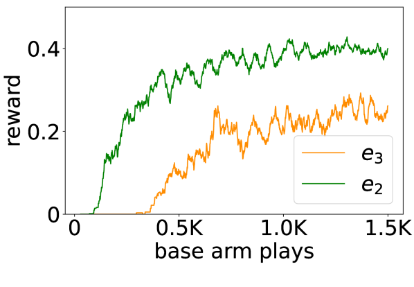
(a) rewards of each arm

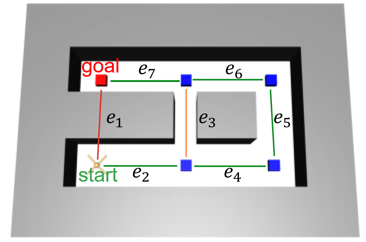
(b) AntMaze-easy

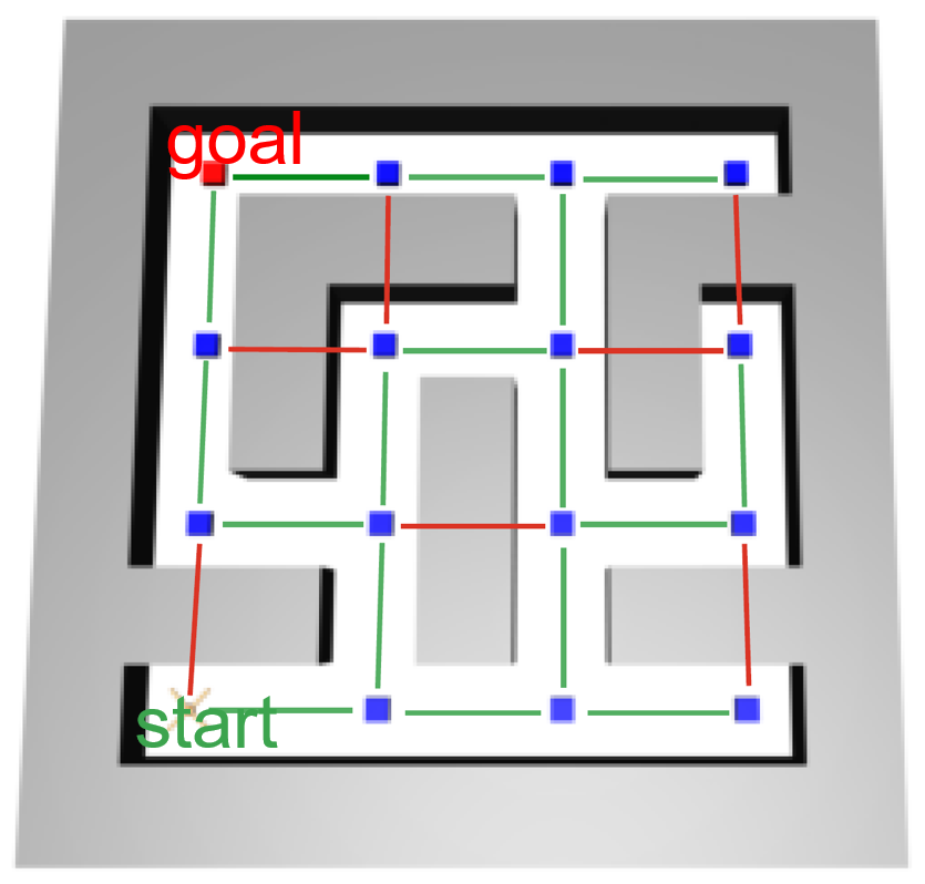
(c) AntMaze-complex

Figure 5: Deep RL environments. (a) We illustrate the rewards of each edge over plays of each arm in AntMaze environments. It is important to note that the rewards are not concave, as they remain at zero until success is achieved. (b, c) We evaluate CRUCB and the baselines in the environments depicted above, where an ant robot navigates the shortest path from the start node to the goal node.

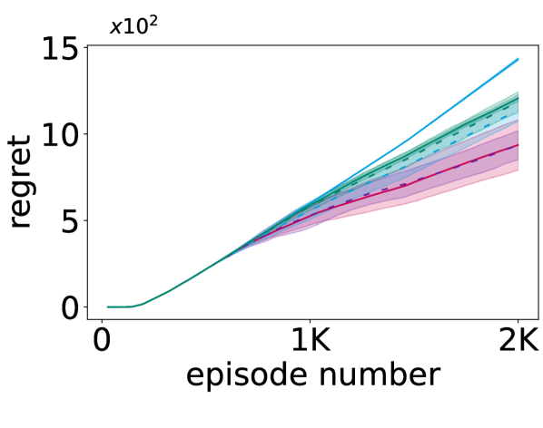
(a) AntMaze-easy

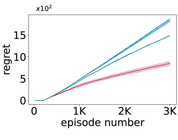
(b) AntMaze-complex

Figure 6: Cumulative regret for each task in deep reinforcement learning environments. We report the average cumulative regret as a line and the 99% confidence interval as a shaded region, based on 3 runs.

6.2 Synthetic environments

We provide experiments for each task based on the complex graph structure depicted in Figure 33(b)-3(d), with graph edges associated with two different types of outcome functions, as illustrated in Figure 3(a). Figure 4 reports the cumulative regret by the oracle constant policy, providing a benchmark for comparison. The results demonstrate that CRUCB consistently outperforms the baseline algorithms across all tasks.

Interestingly, there is a period where the cumulative regret decreases, which is unusual in typical bandit problems. This decrease occurs because, as described in Theorem 1, the oracle policy involves persistently pulling a single optimal super arm, but the optimal super arm changes depending on the episode number. In the early stages with a smaller episode number, it is beneficial to exploit the early peaker since it provides higher immediate rewards. However, as the episode number increases, it becomes more advantageous to switch to the late bloomer, which offers higher cumulative rewards over time. The decrease in cumulative regret is because the optimal policy shifts at the point where the cumulative rewards of the consistently pulling the early peaker and the late bloomer intersect, rather than at the point where the immediate rewards intersect. In contrast, some baselines show nearly zero regret in the early stages, as they fail to capture the rising and continue exploiting the early peaker without sufficient exploration for the late bloomer.

6.3 Deep reinforcement learning

Since deep learning models optimize actions in deep reinforcement learning environments, the performance of the agent naturally improves with training, making it well-suited for the combinatorial rising bandit tasks. Notably, outcomes in reinforcement learning with sparse rewards are often non-concave, primarily due to intervals of zero rewards until the first success is achieved, as illustrated in Figure 5(a).

We conduct experiments on the online shortest path problem using graph-based reinforcement learning in the AntMaze environments, illustrated in Figure 5. The agent solves the problem hierarchically: the high-level agent plans the path, while the low-level agent learns to control the ant robot. As training progresses, the low-level agent’s improved efficiency validates the rising of the outcomes for the high-level agent. Each task emphasizes different aspects: AntMaze-easy focuses on the rising of rewards, while AntMaze-complex focuses the combinatorial nature. There are three types of edges: impossible edge ($e_{1}$), late bloomer ($e_{3}$), and early peaker ($e_{2},e_{4},e_{5},e_{6},e_{7}$). late bloomer ($e_{3}$) initially presents a challenge due to bottleneck but improves over episode, exhibiting rising outcomes. In the early stages, using a detour path composed of easy edges is much efficient, but as training progresses, the late bloomer becomes advantageous to find a shorter path ($e_{2},e_{3},e_{7}$), reducing the cumulative regret. Detailed descriptions of the environments are provided in Appendix B.

(a) optimal policy

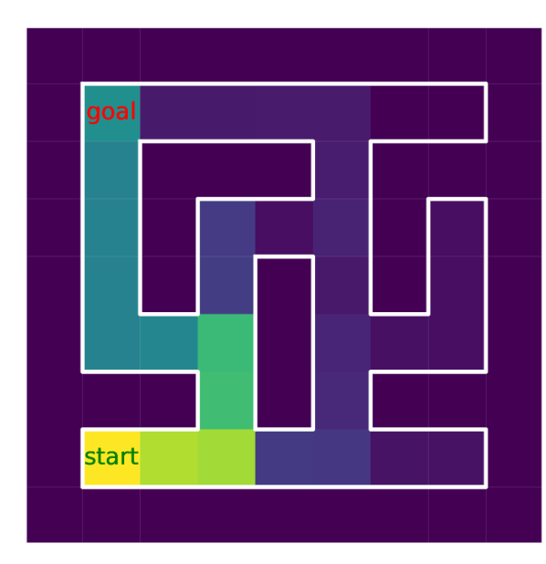
(b) CRUCB (Ours)

(c) R-ed-UCB

Figure 7: Heatmap illustrating visit frequencies in AntMaze-complex. We visualize the visit frequencies across all episodes for the optimal policy, CRUCB, and R-ed-UCB, highlighting the exploration patterns of the agent when operating without prior knowledge of the environment map. Visualizations for the other baselines are provided in Appendix D.

Figure 6(a) shows that CRUCB and R-ed-UCB outperform other baselines in AntMaze-easy, underscoring the significance of considering the rising of rewards in the algorithm design. In AntMaze-complex, CRUCB maintains its superior performance, as shown in Figure 6(b). The heatmap in Figure 7 further reveals that CRUCB primarily focuses on exploring and exploiting the optimal path to the goal, while R-ed-UCB distributes its exploration across all paths. R-ed-UCB would pose challenges in environments where the number of super arms increases significantly. Notably, CRUCB outperforms even when the outcomes are not concave, demonstrating its broader applicability in practice.

7 Conclusion

In this paper, we proposed CRUCB for the combinatorial rising bandit. We provided theoretical guarantees by deriving the regret upper bound for CRUCB’s performance and establishing tightness with the regret lower bound. Our experimental results on diverse environments validate the effectiveness of CRUCB. However, a limitation of our current work is the assumption of additive rewards in Assumption 1, which may not capture the complexity of all practical scenarios. Future research could extend this work to address general reward settings, potentially leading to more versatile solutions for a wider range of real-world problems.

This material provides proof of theorems, details of environments and baselines, and additional experimental results:

• Appendix A: Proofs of Theorem 1, 3, 4, and 5.

• Appendix B: Detailed description of environments in Section 6.

• Appendix C: Detailed description and pseudocode of baselines in Section 6.

• Appendix D: Further analysis of exploration heatmap in Figure 7 on other baselines.

Appendix A Proof of theorems

A.1 Proof of Theorem 1

We show that for any combinatorial rising bandit problem, some constant policy, which is pulling one super arm continuously, is optimal, meaning that it maximizes the expected cumulative reward, which is defined in (4).

Set up.

Fix a combinatorial rising bandit problem $\bm{\mu}$ with $K$ base arms and super arm set $\mathcal{S}$, and total time $T$. By Assumption 1, the cumulative reward is invariant with respect to permutations of the order of pulling super arms, which means that a policy can be represented as the vector of number of pulling each super arm. That is, a policy $\pi$ can be represented as follows:

$$\pi\mapsto\left(T^{\pi}_{1},T^{\pi}_{2},\cdots,T^{\pi}_{|\mathcal{S}|}\right)\;,$$ (26)

where $T^{\pi}_{S}$ denotes the number of pulling a super arm $S$ until time $T$ by the policy $\pi$, which satisfies $\sum_{S\in\mathcal{S}}T^{\pi}_{S}=T$. Let $N^{\pi}_{i,T}$ denote the number of pulling a base arm $i$ until time $T$ by $\pi$. Then, $N^{\pi}_{i,T}$ can be represented as follows:

$$N^{\pi}_{i,T}=\sum_{S\in\mathcal{S}}T^{\pi}_{S}\mathds{1}\left\{i\in S\right\}\;,$$ (27)

where $\mathds{1}$ denotes the indicator function. Let $\pi^{*}$ be the optimal policy given the problem $\bm{\mu}$ and $T$. Suppose $\pi^{*}$ be the optimal policy given the problem $\bm{\mu},\mathcal{S}$, and $T$. We show that if $\pi^{*}$ pulls at least two different super arms, then a constant policy, which is pulling one super arm continuously, can be constructed so that generates the same expected cumulative reward as the one produced by $\pi^{*}$, which suffices to conclude.

Assume that $\pi^{*}$ selects $m$ distinct super arms, denote by super arms as $S_{1},S_{2},\ldots,S_{m}$. Define a subset of base arms $B_{c}$ and $B_{j}$ for each $j\in[K]$ as follows:

$$B_{c}:=\left\{i\in[K]\mid i\in S_{j}\quad\forall j\in[K]\right\}\;;$$ (28)

$$B_{j}:=S_{j}\setminus B_{c}\;.$$ (29)

$B_{c}$ represents the subset of the common base arms included in every selected super arm by the optimal policy $\pi^{*}$ and $B_{j}$ represents the subset of base arms included in the super arm $S_{j}$ except for $B_{c}$.

Claim 1.

$\sum_{i\in B_{j}}\mu_{i}(N^{\pi^{*}}_{i,T})$ is equal for all $j\in[K]$.

Proof.

To establish Claim 1, we consider two arbitrary distinct super arms, $S_{1}$ and $S_{2}$, without loss of generality. We observe $\sum_{i\in B_{1}\setminus B_{2}}\mu_{i}(N^{\pi^{*}}_{i,T})\geq\sum_{i\in B_{2}\setminus B_{1}}\mu_{i}(N^{\pi^{*}}_{i,T})$. If not, that is, $\sum_{i\in B_{1}\setminus B_{2}}\mu_{i}(N^{\pi^{*}}_{i,T})<\sum_{i\in B_{2}\setminus B_{1}}\mu_{i}(N^{\pi^{*}}_{i,T})$, we can construct new policy $\pi_{1}$ as follows:

$$T^{\pi_{1}}_{S}=\begin{cases}T^{\pi^{*}}_{S_{1}}-1&S=S_{1}\;;\\ T^{\pi^{*}}_{S_{2}}+1&S=S_{2}\;;\\ T^{\pi^{*}}_{S}&\text{otherwise}.\\ \end{cases}$$ (30)

Then, $N^{\pi_{1}}_{i,T}$ is given by:

$$N^{\pi_{1}}_{i,T}=\begin{cases}N^{\pi^{*}}_{i,T}-1&i\in B_{1}\setminus B_{2}\;;\\ N^{\pi^{*}}_{i,T}+1&i\in B_{2}\setminus B_{1}\;;\\ N^{\pi^{*}}_{i,T}&\text{otherwise}\;.\\ \end{cases}$$ (31)

The difference between the expected cumulative reward of $\pi^{*}$ and $\pi_{1}$ is given by:

$$\quad\sum_{i\in[K]}\left(\sum_{n\in[N^{\pi^{*}}_{i,T}]}\mu_{i}(n)-\sum_{n\in[N^{\pi_{1}}_{i,T}]}\mu_{i}(n)\right)$$ (32)

$$=\sum_{i\in B_{1}\setminus B_{2}}\mu_{i}(N^{\pi^{*}}_{i,T})-\sum_{i\in B_{2}\setminus B_{1}}\mu_{i}(N^{\pi^{*}}_{i,T}+1)\;$$ (33)

$$<0\;,$$ (34)

which indicates that the cumulative reward of $\pi_{1}$ is larger than that of $\pi^{*}$. However, it is contradicting with the assumption that $\pi^{*}$ is optimal and thus we have $\sum_{i\in B_{1}\setminus B_{2}}\mu_{i}(N^{\pi^{*}}_{i,T})\geq\sum_{i\in B_{2}\setminus B_{1}}\mu_{i}(N^{\pi^{*}}_{i,T})$. By applying the same logic, we can also derive that $\sum_{i\in B_{1}\setminus B_{2}}\mu_{i}(N^{\pi^{*}}_{i,T})\leq\sum_{i\in B_{2}\setminus B_{1}}\mu_{i}(N^{\pi^{*}}_{i,T})$. We have $\sum_{i\in B_{1}\setminus B_{2}}\mu_{i}(N^{\pi^{*}}_{i,T})=\sum_{i\in B_{2}\setminus B_{1}}\mu_{i}(N^{\pi^{*}}_{i,T})$. By adding $\sum_{i\in B_{1}\cap B_{2}}\mu_{i}(N^{\pi^{*}}_{i,T})$, we can derive that $\sum_{i\in B_{1}}\mu_{i}(N^{\pi^{*}}_{i,T})=\sum_{i\in B_{2}}\mu_{i}(N^{\pi^{*}}_{i,T})$. Since we can apply the same logic to any arbitrary super arm pair, we can conclude the claim. ∎

Claim 2.

$\sum_{i\in B_{j}\setminus B_{j^{\prime}}}\mu_{i}(N^{\pi^{*}}_{i,T}-T^{\pi^{*}}_{S_{1}}+1)=\sum_{i\in B_{j}\setminus B_{j^{\prime}}}\mu_{i}(N^{\pi^{*}}_{i,T})$ for any $j,\;j^{\prime}\in[K]$ .

Proof.

Similar to Claim 1, we consider $S_{1}$ and $S_{2}$ without loss of generality. Given that $\sum_{i\in B_{1}\setminus B_{2}}\mu_{i}(N^{\pi^{*}}_{i,T})\leq\sum_{i\in B_{2}\setminus B_{1}}\mu_{i}(N^{\pi^{*}}_{i,T})$ from preceding analysis, we observe $\sum_{i\in B_{1}\setminus B_{2}}\mu_{i}(N^{\pi^{*}}_{i,T}-T^{\pi^{*}}_{S_{1}}+1)\geq\sum_{i\in B_{2}\setminus B_{1}}\mu_{i}(N^{\pi^{*}}_{i,T})$. Otherwise, that is, $\sum_{i\in B_{1}\setminus B_{2}}\mu_{i}(N^{\pi^{*}}_{i,T}-T^{\pi^{*}}_{S_{1}}+1)<\sum_{i\in B_{2}\setminus B_{1}}\mu_{i}(N^{\pi^{*}}_{i,T})$, we can construct new policy $\pi_{2}$ such that:

$$T^{\pi_{2}}_{S}=\begin{cases}0&S=S_{1}\;;\\ T^{\pi^{*}}_{S_{1}}+T^{\pi^{*}}_{S_{2}}&S=S_{2}\;;\\ T^{\pi^{*}}_{S}&\text{otherwise}.\\ \end{cases}$$ (35)

Then, $N^{\pi_{2}}_{i,T}$ is given by:

$$N^{\pi_{2}}_{i,T}=\begin{cases}N^{\pi^{*}}_{i,T}-T^{\pi^{*}}_{S_{1}}&i\in B_{1}\setminus B_{2}\;;\\ N^{\pi^{*}}_{i,T}+T^{\pi^{*}}_{S_{1}}&i\in B_{2}\setminus B_{1}\;;\\ N^{\pi^{*}}_{i,T}&\text{otherwise}.\\ \end{cases}$$ (36)

The difference between the cumulative rewards of $\pi^{*}$ and $\pi_{2}$ is given by:

$$\sum_{i\in[K]}\left(\sum_{n\in[N^{\pi^{*}}_{i,T}]}\mu_{i}(n)-\sum_{n\in[N^{\pi_{2}}_{i,T}]}\mu_{i}(n)\right)$$ (37)

$$= \sum_{i\in B_{1}\setminus B_{2}}\sum_{n=N^{\pi^{*}}_{i,T}-T^{\pi^{*}}_{S_{1}}+1}^{N^{\pi^{*}}_{i,T}}\mu_{i}(n)-\sum_{i\in B_{2}\setminus B_{1}}\sum_{n=N^{\pi^{*}}_{i,T}+1}^{N^{\pi^{*}}_{i,T}+T^{\pi^{*}}_{S_{1}}}\mu_{i}(n)$$ (38)

$$= \sum_{l=1}^{T^{\pi^{*}}_{S_{1}}}\left(\sum_{i\in B_{1}\setminus B_{2}}\mu_{i}(N^{\pi^{*}}_{i,T}-T^{\pi^{*}}_{S_{1}}+l)-\sum_{i\in B_{2}\setminus B_{1}}\mu_{i}(N^{\pi^{*}}_{i,T}+l)\right)$$ (39)

$$\leq \left(\sum_{i\in B_{1}\setminus B_{2}}\mu_{i}(N^{\pi^{*}}_{i,T}-T^{\pi^{*}}_{S_{1}}+1)-\sum_{i\in B_{2}\setminus B_{1}}\mu_{i}(N^{\pi^{*}}_{i,T})\right)+(T^{\pi^{*}}_{S_{1}}-1)\left(\sum_{i\in B_{1}\setminus B_{2}}\mu_{i}(N^{\pi^{*}}_{i,T})-\sum_{i\in B_{2}\setminus B_{1}}\mu_{i}(N^{\pi^{*}}_{i,T})\right)$$ (40)

$$< 0\;,$$ (41)

where (39) holds since $\mu_{i}(N^{\pi^{*}}_{i,T}-T^{\pi^{*}}_{S_{1}}+l)\leq\mu_{i}(N^{\pi^{*}}_{i,T})$ and $\mu_{i}(N^{\pi^{*}}_{i,T}+l)>\mu_{i}(N^{\pi^{*}}_{i,T})$ for any $l\in[2,T^{\pi^{*}}_{S_{1}}]$ for any base arm $i$ by the definition of combinatorial rising bandit. It indicates that the cumulative reward of $\pi_{2}$ is larger than that of $\pi^{*}$, which is a contradiction with assumption that $\pi^{*}$ is optimal. Therefore, we have $\sum_{i\in B_{1}\setminus B_{2}}\mu_{i}(N^{\pi^{*}}_{i,T}-T^{\pi^{*}}_{S_{1}}+1)\geq\sum_{i\in B_{2}\setminus B_{1}}\mu_{i}(N^{\pi^{*}}_{i,T})$. Combining this observation with the previous observation, we have $\sum_{i\in B_{1}\setminus B_{2}}\mu_{i}(N^{\pi^{*}}_{i,T}-T^{\pi^{*}}_{S_{1}}+1)=\sum_{i\in B_{1}\setminus B_{2}}\mu_{i}(N^{\pi^{*}}_{i,T})$. This result implies that rewards of all base arms in $S_{1}$ are flat after pulling for $N^{\pi^{*}}_{i,T}-T^{\pi^{*}}_{S_{1}}$ times. Since we can apply the same logic to any arbitrary super arm pair, we can conclude the claim. ∎

Induction.

Lastly, we construct constant policy inductively. As before, we choose two arbitrary two super arm and consider $S_{1}$ and $S_{2}$ without loss of generality. we revisit $\pi_{2}$. By Claim 1 and Claim 2 the difference between $\pi^{*}$ and $\pi_{2}$ equals 0, which means that $\pi_{2}$ is also an optimal policy. We remark that $\pi_{2}$ plays $m-1$ distinct super arms. Applying preceding logic inductively, we can construct the optimal policy pulls only one super arm, which completes proof.

A.2 Proof of Theorem 3

Proof.

For any super arm $S$, define $B_{S}(t)$ and $\mu_{S}(t)$ as follows:

$$B_{S}(t):=\sum_{i\in S}\left(\hat{\mu}_{i}(t)+\beta_{i}(t)\right)\;;$$ (42)

$$\mu_{S}(t):=\sum_{i\in S}\mu_{i}(N_{i,t})\;.$$ (43)

To define well-estimated event, we define $\hat{\mu}_{i}(t)$ and $\widetilde{\mu}_{i}(t)$ as follows:

$$\hat{\mu}_{i}(t):=\frac{1}{h_{i}}\sum_{l=N_{i,t-1}-h_{i}+1}^{N_{i,t-1}}\left(X_{i}(l)+(t-l)\frac{X_{i}(l)-X_{i}(l-h_{i})}{h_{i}}\right)\;;$$ (44)

$$\widetilde{\mu}_{i}(t):=\frac{1}{h_{i}}\sum_{l=N_{i,t-1}-h_{i}+1}^{N_{i,t-1}}\left(\mu_{i}(l)+(t-l)\frac{\mu_{i}(l)-\mu_{i}(l-h_{i})}{h_{i}}\right)\;;$$ (45)

$$\beta_{i}(t):=\sigma\left(t-N_{i,t-1}+h_{i}-1\right)\sqrt{\frac{10\log t^{3}}{h_{i}^{3}}}\;.$$ (46)

We define well-estimated event $\mathcal{E}_{t}$ as follows:

$$\mathcal{E}_{i,t}:=\left\{|\hat{\mu}_{i}(t)-\widetilde{\mu}_{i}(t)|\leq\beta_{i}(t)\right\}\;;$$ (47)

$$\mathcal{E}_{t}:=\cap_{i\in[K]}\mathcal{E}_{i,t}\;.$$ (48)

For simplicity, we refer to the optimal super arm $S^{{\dagger}}(\bm{\mu},T)$ as $S^{{\dagger}}$. In CRUCB, the Solver selects the super arm $S_{t}$ with the largest $B_{S_{t}}(t)$, which implies that $B_{S^{{\dagger}}}(t)\leq B_{S_{t}}(t)$. We decompose the regret with well-estimated event $\mathcal{E}_{t}$.

$$R_{\bm{\mu}}(\pi,T) =\mathbb{E}_{S_{t}\sim\pi^{*}}\left[\sum_{t\in[T]}X_{S_{t}}(t)\right]-\mathbb{E}_{S_{t}\sim\pi}\left[\sum_{t\in[T]}X_{S_{t}}(t)\right]$$ (49)

$$=\sum_{t\in[T]}\mathbb{E}\left[X_{S^{{\dagger}}}(t)-X_{S_{t}}(t)\right]$$ (50)

$$=\sum_{t\in[T]}\mathbb{E}\left[\left(X_{S^{{\dagger}}}(t)-X_{S_{t}}(t)\right)\mathds{1}\{\lnot\mathcal{E}_{t}\}\right]+\sum_{t\in[T]}\mathbb{E}\left[\left(X_{S^{{\dagger}}}(t)-X_{S_{t}}(t)\right)\mathds{1}\{\mathcal{E}_{t}\}\right]$$ (51)

$$\leq\underbrace{L\sum_{t\in[T]}\mathbb{E}\left[\mathds{1}\{\lnot\mathcal{E}_{t}\}\right]}_{(A)}+\underbrace{\sum_{t\in[T]}\mathbb{E}\left[\left(X_{S^{{\dagger}}}(t)-X_{S_{t}}(t)\right)\mathds{1}\{\mathcal{E}_{t}\}\right]}_{(B)}\;.$$ (52)

To bound term (A), we borrow concentration inequality from (Metelli et al. 2022).

Lemma 1.

(Metelli et al. 2022) For every round $K<t<T$, and window size $1\leq h_{i}\leq\varepsilon N_{i,t-1}$, we have:

$$\mathbb{P}(\lnot\mathcal{E}_{t})\leq\frac{2K}{t^{2}}\;.$$ (53)

Now, we bound term (A).

$$\underbrace{L\sum_{t\in[T]}\mathbb{E}\left[\mathds{1}\{\lnot\mathcal{E}_{t}\}\right]}_{(A)} =L\sum_{t\in[T]}\mathbb{P}(\lnot\mathcal{E}_{t})$$ (54)

$$\leq\sum_{t\in[T]}\frac{2LK}{t^{2}}$$ (55)

$$\leq\frac{L\pi K}{3}\;,$$ (56)

Now, we bound term (B), which measures the regret occurred when all base arms are well-estimated. We decompose the inner term of term (B) into two parts:

$$\underbrace{\mathbb{E}\left[\left(X_{S^{{\dagger}}}(t)-X_{S_{t}}(t)\right)\right]}_{\text{inner term of term }(B)} =\mu_{S^{{\dagger}}}(t)-\mu_{S_{t}}(t)-B_{S_{t}}(t)+B_{S_{t}}(t)$$ (57)

$$\leq B_{S_{t}}(t)-\mu_{S_{t}}(t)$$ (58)

$$=\sum_{i\in S_{t}}\hat{\mu}_{i}(t)+\beta_{i}(t)-\mu_{i}(t)$$ (59)

$$\leq\sum_{i\in S_{t}}\underbrace{\widetilde{\mu}_{i}(t)-\mu_{i}(t)}_{(B1)}+\underbrace{2\beta_{i}(t)}_{(B2)}\;,$$ (60)

where (58) holds from the definition of $B_{S_{t}}(t)$ and (60) holds since the term (B) is under the event $\mathcal{E}_{t}$. We bound the term (B1) defining $t_{i,n}$ as the time step where the base arm $i$ is pulled the $n^{\text{th}}$ time:

$$\sum_{t=1}^{T}\sum_{i\in S_{t}}\widetilde{\mu}_{i}(t)-\mu_{i}(t) \leq 2K+\sum_{i\in[K]}\sum_{n=3}^{N_{i,t}}\min\left\{\widetilde{\mu}_{i}(t_{i,n},n)-\mu_{i}(t),1\right\}$$ (61)

$$\leq 2K+\sum_{i\in[K]}\sum_{n=3}^{N_{i,t}}\min\left\{\frac{1}{2}(2t_{i,n}-2n+h_{i}-1)\gamma_{i}(n-2h_{i}+1),1\right\}$$ (62)

$$=2K+\sum_{i\in[K]}\sum_{n=3}^{N_{i,t}}\min\left\{T\gamma_{i}((1-2\varepsilon)n),1\right\}$$ (63)

$$\leq 2K+T^{q}\sum_{i\in[K]}\sum_{n=3}^{N_{i,t}}\gamma_{i}((1-2\varepsilon)n)^{q}$$ (64)

$$\leq 2K+KT^{q}(\frac{1}{1-2\varepsilon})\Upsilon\left((1-2\varepsilon)\frac{LT}{K},q\right),$$ (65)

where (62) follows from the Lemma A.3, in (Metelli et al. 2022), (64) follows from the fact $\min(s,1)\leq\min(s,1)^{q}\leq s^{q}$ for $q\in[0,1]$, and (65) follows from the Lemma C.2. in (Metelli et al. 2022). Now, we bound the term (B2).

$$\sum_{t=1}^{T}\sum_{i\in S_{t}}2\min\left\{\beta_{i}(t),1\right\} =\sum_{t=1}^{T}\sum_{i\in S_{t}}2\min\left\{\sigma\left(t-N_{i,t-1}+h_{i}-1\right)\sqrt{\frac{2\log 4t^{3}}{h^{3}}},1\right\}$$ (66)

$$\leq\sum_{t=1}^{T}\sum_{i\in S_{t}}2\min\left\{T\sigma\sqrt{\frac{6\log 4T}{\left(\varepsilon\lfloor N_{i,t}\rfloor\right)^{3}}},1\right\}$$ (67)

$$=\sum_{i\in[K]}\sum_{n=1}^{N_{i,t}}2\min\left\{T\sigma\sqrt{\frac{6\log 4T}{\left(\varepsilon\lfloor n\rfloor\right)^{3}}},1\right\}\;.$$ (68)

Choose $n^{\prime}=\frac{(2\sigma T)^{\frac{2}{3}}\left(6\log(4T)\right)^{\frac{1}{3}}}{\varepsilon}$. Then for $n>n^{\prime}$

$$2\sigma T\sqrt{\frac{6\log 4T}{\left(\varepsilon\lfloor n\rfloor\right)^{3}}}\leq 1\;.$$ (69)

Thus, we have:

$$\sum_{i\in[K]}\sum_{n=1}^{N_{i,t}}2\min\left\{\sigma T\sqrt{\frac{6\log 4T}{\left(\varepsilon\lfloor n\rfloor\right)^{3}}},1\right\} \leq\sum_{i\in[K]}\left(n^{\prime}+\sum_{n=n^{\prime}+1}^{T}T\sqrt{\frac{6\log 4T}{\left(\varepsilon\lfloor n\rfloor\right)^{3}}}\right)$$ (70)

$$\leq K\left(n^{\prime}+2\sigma T\sqrt{\frac{6\log 4T}{\varepsilon^{3}}}\int_{n^{\prime}}^{\infty}x^{-\frac{3}{2}}dx\right)$$ (71)

$$=O(T^{\frac{2}{3}}\log T^{\frac{1}{3}})\;,$$ (72)

where (71) comes from the fact that the sum of monotone decreasing function can be upper bounded. Combining the results from (56), (65), and (72), we conclude the proof. ∎

A.3 Proof of Theorem 4

Proof.

For simplicity, we represent the number of pulling super arm $S$ until time $t$, we introduce the notation $N_{S,t}$, following the same convention as $N_{i,t}$ for a base arm $i$. To distinguish two distinct problems, we denote the expectation of random variable $X$ under policy $\pi$ on problem $\bm{\mu}$ as $\mathbb{E}_{\bm{\mu},\pi}[X]$. Firstly, we consider non-combinatorial case. We construct two different problems and show that no policy can achieve sub-linear regret for both problem as other works.

Lemma 2.

Let $\mathcal{I^{\prime}}$ be the set of all available two-armed rising bandit problem. For sufficiently large time $T$, any policy $\pi$ suffers regret:

$$\min_{\pi}\max_{\bm{\mu}\in\mathcal{I^{\prime}}}R_{\bm{\mu}}(\pi,T)\geq\frac{T}{32}\;,$$ (73)

Proof.

For simplicity, we consider the deterministic problem, that is, $\sigma=0$. Define two problem $\bm{\mu^{A}}$ and $\bm{\mu^{B}}$ as follows:

$$\mu^{A}_{1}(n)=\mu^{B}_{1}(n)=\frac{1}{2}\;;$$

$$\mu^{A}_{2}(n)=\begin{cases}\frac{3n}{2T}&\text{if }n\leq\frac{2T}{3}\\ 1&\text{otherwise}\end{cases}\;;$$

$$\mu^{B}_{2}(n)=\begin{cases}\frac{3n}{2T}&\text{if }n\leq\frac{T}{3}\\ \frac{1}{2}&\text{otherwise}\end{cases}\;.$$

In this setting, we define $\mathcal{S}$ as follows:

$$\mathcal{S}=\left\{S_{1},S_{2}\right\}\;.$$ (74)

For simplicity, we denote super arm $\{1\}$ as $S_{1}$ and $\{2\}$ as $S_{2}$. The main idea of the proof is that for any arbitrary policy $\pi^{\prime}$, the agent receives the same rewards for both $\bm{\mu^{A}}$ and $\bm{\mu^{B}}$ at least until $\frac{T}{3}$, indicating that:

$$\mathbb{E}_{\bm{\mu}^{A},\pi^{\prime}}\left[N_{S_{1},\frac{T}{3}}\right]=\mathbb{E}_{\bm{\mu}^{B},\pi^{\prime}}\left[N_{S_{1},\frac{T}{3}}\right]=:s\;.$$ (75)

Fix some arbitrary policy $\pi$. We compute the cumulative regret of policy $\pi$ in $\bm{\mu^{A}}$ and $\bm{\mu^{B}}$.

Case (A)

For $\bm{\mu^{A}}$, the optimal super arm is $S_{2}$, and the corresponding cumulative reward is given by:

$$\mathbb{E}_{\bm{\mu}^{A},\pi}\left[\sum_{t\in T}X_{S_{t}}(t)\right]=\sum_{n=1}^{\frac{2T}{3}}\frac{3n}{2T}+\frac{T}{3}\;.$$ (76)

For the given policy $\pi$, the cumulative reward is upper bounded as follows:

$$\mathbb{E}_{\bm{\mu}^{A},\pi}\left[\sum_{t\in T}X_{S_{t}}(t)\right] =\frac{1}{2}\mathbb{E}_{\bm{\mu}^{A},\pi}[N_{S_{1},T}]+\sum_{n=1}^{T-\mathbb{E}_{\bm{\mu}^{A},\pi}[N_{S_{1},T}]}\mu^{A}_{2}(n)$$ (77)

$$\leq\frac{s}{2}+\sum_{n=1}^{T-s}\mu^{A}_{2}(n)$$ (78)

$$=\frac{s}{2}+\sum_{n=1}^{\frac{2T}{3}}\frac{3n}{2T}+\left(\frac{T}{3}-s\right)$$ (79)

$$=\sum_{n=1}^{\frac{2T}{3}}\frac{3n}{2T}+\frac{T}{3}-\frac{s}{2}\;,$$ (80)

where (78) holds since the cumulative reward is maximized as $\mathbb{E}_{\bm{\mu}^{A},\pi}[N_{S_{1},T}]$ minimized and it is guaranteed that $\mathbb{E}_{\bm{\mu}^{A},\pi}[N_{S_{1},T}]\geq\mathbb{E}_{\bm{\mu}^{A},\pi}[N_{S_{1},\frac{T}{3}}]=s$.

The cumulative regret is lower bounded by:

$$R_{\bm{\mu^{A}}}(\pi,T) \geq\sum_{n=1}^{\frac{2T}{3}}\frac{3n}{2T}+\frac{T}{3}-\left(\sum_{n=1}^{\frac{2T}{3}}\frac{3n}{2T}+\frac{T}{3}-\frac{s}{2}\right)$$ (81)

$$=\frac{s}{2}\;.$$ (82)

Case (B)

For $\bm{\mu^{B}}$, the optimal super arm is $S_{1}$, and the corresponding cumulative reward is given by:

$$\mathbb{E}_{\bm{\mu}^{B},\pi}\left[\sum_{t\in T}X_{S_{t}}(t)\right]=\frac{T}{2}\;.$$ (83)

For the given policy $\pi$, the cumulative reward is upper bounded as follows:

$$\mathbb{E}_{\bm{\mu}^{B},\pi}\left[\sum_{t\in T}X_{S_{t}}(t)\right] =\frac{1}{2}\mathbb{E}_{\bm{\mu}^{B},\pi}[N_{S_{1},T}]+\sum_{n=1}^{T-\mathbb{E}_{\bm{\mu}^{B},\pi}[N_{S_{1},T}]}\mu^{B}_{2}(n)$$ (84)

$$\leq\frac{(\frac{2T}{3}+s)}{2}+\sum_{n=1}^{\frac{T}{3}-s}\mu^{B}_{2}(n)$$ (85)

$$=\sum_{n=1}^{\frac{T}{3}-s}\frac{3n}{2T}+\frac{T}{3}+\frac{s}{2}$$ (86)

$$=\frac{3}{4T}\left(\frac{T}{3}-s\right)\left(\frac{T}{3}-s+1\right)+\frac{T}{3}+\frac{s}{2}$$ (87)

$$=\frac{3s^{2}}{4T}-\frac{3s}{4T}+\frac{5T}{12}+\frac{1}{4}\;,$$ (88)

where (78) holds since the cumulative reward is maximized as $\mathbb{E}_{\bm{\mu}^{A},\pi}[N_{S_{1},T}]$ maximized and it is guaranteed that $\mathbb{E}_{\bm{\mu}^{B},\pi}[N_{S_{1},T}]\leq\frac{2T}{3}+\mathbb{E}_{\bm{\mu}^{B},\pi}[N_{S_{1},\frac{T}{3}}]=\frac{2T}{3}+s$.

The cumulative regret is lower bounded by:

$$R_{\bm{\mu^{B}}}(\pi,T) \geq\frac{T}{2}-\left(\frac{3s^{2}}{4T}-\frac{3s}{4T}+\frac{5T}{12}+\frac{1}{4}\right)$$ (89)

$$=-\frac{3s^{2}}{4T}+\frac{3s}{4T}+\frac{T}{12}-\frac{1}{4}$$ (90)

$$\geq-\frac{3s^{2}}{4T}+\frac{3s}{4T}+\frac{T}{16}\;,$$ (91)

where (91) holds since we assume sufficiently large $T$.

From previous results, the worst-case regret can be lower bounded as follows:

$$\inf_{\pi}\sup_{\bm{\mu}}R_{\bm{\mu}}(\pi,T) \geq\inf_{\pi}\max\left\{R_{\bm{\mu}^{A}}(\pi,T),R_{\bm{\mu}^{B}}(\pi,T)\right\}$$ (92)

$$=\inf_{s\in\left[0,\frac{T}{3}\right]}\max\left\{\frac{Ls}{2},-\frac{3s^{2}}{4T}+\frac{3s}{4T}+\frac{T}{16}\right\}$$ (93)

$$\geq\inf_{s\in\left[0,\frac{T}{3}\right]}\frac{-12s^{2}+(8T+12)s+T^{2}}{32T})$$ (94)

$$\geq\frac{T}{32}\;,$$ (95)

where (94) holds since $\max(a,b)\geq\frac{a+b}{2}$ and (95) holds since it is easily verified that (94) is minimized when $s=0$, which completes the proof. ∎

Now, we expand Lemma 2 to general combinatorial setting. Let $L$ be an arbitrary constant. We define two problem $\bm{\mu^{A,L}}$ and $\bm{\mu^{B,L}}$ construct super arm set $\mathcal{S}_{L}$ as follows:

$$\mu^{A,L}_{i}(n)=\mu^{B,L}_{i}(n)=\frac{1}{2}\quad i\in[1,L]$$ (96)

$$\mu^{A,L}_{i}(n)=\begin{cases}\frac{3n}{2T}&\text{if }n\leq\frac{2T}{3}\\ 1&\text{otherwise}\end{cases}\quad i\in[L+1,2L]$$ (97)

$$\mu^{B,L}_{i}(n)=\begin{cases}\frac{3n}{2T}&\text{if }n\leq\frac{T}{3}\\ \frac{1}{2}&\text{otherwise}\end{cases}\quad i\in[L+1,2L]\;$$ (98)

$$S_{L}:=\left\{(a_{1},a_{2},\ldots,a_{L}):a_{i}\in\{i,L+i\}\quad i\in[L]\right\}\;.$$ (99)

Since it can be interpreted as solving $L$ independent problems, we have:

$$\inf_{\pi}\sup_{\bm{\mu}}R_{\bm{\mu}}(\pi,T)\geq\frac{LT}{32}\;.$$ (100)

∎

A.4 Proof of Theorem 5

Proof.

We apply similar logic given in the Appendix A.3 to show that for the worst-case lower bound is $O(LT^{2-c})$. Firstly, we consider non-combinatorial case.

Lemma 3.

Let $\mathcal{A}^{\prime}_{c}$ be the subset of two-armed rising bandit problem with constraints given in (24) . For sufficiently large time $T$, any policy $\pi$ suffers regret:

$$\min_{\pi}\max_{\bm{\mu}\in\mathcal{A}^{\prime}_{c}}R_{\bm{\mu}}(\pi,T)\geq LT^{2-c}\;,$$ (101)

Proof.

For convention, we define $\mu(m)$ and $F(m)$ as follows:

$$\mu(m):=\sum_{n=1}^{m}(n+1)^{-c}\;;$$ (102)

$$F(m):=\sum_{n=1}^{m}\mu(n)\;.$$ (103)

Let $\bm{\mu^{A}}$ and $\bm{\mu^{B}}$ be two rising bandit instances. which are defined as:

$$\mu^{A}_{1}(n)=\mu^{B}_{2}(n)=\mu(P)-\varepsilon\;;$$ (104)

$$\mu^{A}_{2}(n)=\mu(n)\;;$$ (105)

$$\mu^{B}_{2}(n)=\begin{cases}\mu(n)&\text{if }n\leq P\\ \mu(P)&\text{otherwise}\end{cases}\;,$$ (106)

where $P=(2-c)^{\frac{1}{c-1}}T$ and $0<\varepsilon<\mu(P)$ will be specified later. In this setting, we define $\mathcal{S}$ as follows:

$$\mathcal{S}=\left\{S_{1},S_{2}\right\}\;,$$ (107)

where $S_{1}=\{1\}$ and $S_{2}=\{2\}$. We note that $\bm{\mu^{A}}$ and $\bm{\mu^{B}}$ belongs to $\mathcal{A}^{\prime}_{c}$. We firstly assume that the optimal super arm for $\bm{\mu}^{A}$ is $S_{2}$ and the optimal super arm for $\bm{\mu}^{B}$ is $S_{1}$. We will show that it is true after $\varepsilon$ is specified.

The main idea of the proof is that for any arbitrary policy $\pi^{\prime}$, the agent receives the same rewards for both $\bm{\mu^{A}}$ and $\bm{\mu^{B}}$ at least until $P$, indicating that:

$$\mathbb{E}_{\bm{\mu}^{A},\pi^{\prime}}\left[N_{S_{1},P}\right]=\mathbb{E}_{\bm{\mu}^{B},\pi^{\prime}}\left[N_{S_{1},P}\right]=:s\;.$$ (108)

Case (A)

For $\bm{\mu^{A}}$, the optimal super arm is $S_{2}$, and the corresponding cumulative reward is given by:

$$\mathbb{E}_{\bm{\mu}^{A},\pi}\left[\sum_{t\in T}X_{S_{t}}(t)\right]=F(T)\;.$$ (109)

For the given policy $\pi$, the cumulative reward is upper bounded as follows:

$$\mathbb{E}_{\bm{\mu}^{A},\pi}\left[\sum_{t\in T}X_{S_{t}}(t)\right] =\left(\mu(P)-\varepsilon\right)\mathbb{E}_{\bm{\mu}^{A},\pi}[N_{S_{1},T}]+\sum_{n=1}^{T-\mathbb{E}_{\bm{\mu}^{A},\pi}[N_{S_{1},T}]}\mu^{A}_{2}(n)$$ (110)

$$\leq\left(\mu(P)-\varepsilon\right)s+F(T-s),$$ (111)

where (111) holds since the cumulative reward is maximized as $\mathbb{E}_{\bm{\mu}^{A},\pi}[N_{S_{1},T}]$ minimized and it is guaranteed that $\mathbb{E}_{\bm{\mu}^{A},\pi}[N_{S_{1},T}]\geq\mathbb{E}_{\bm{\mu}^{A},\pi}[N_{S_{1},P}]=s$.

With The cumulative regret is lower bounded by:

$$R_{\bm{\mu^{A}}}(\pi,T) \geq F(T)-\left(\mu(P)-\varepsilon\right)s-F(T-s)\;.$$ (112)

Case (B)

For $\bm{\mu^{B}}$, the optimal super arm is $S_{1}$, and the corresponding cumulative reward is given by:

$$\mathbb{E}_{\bm{\mu}^{B},\pi}\left[\sum_{t\in T}X_{S_{t}}(t)\right]=T\left(\mu(P)-\varepsilon\right)\;.$$ (113)

For the given policy $\pi$, the cumulative reward is upper bounded as follows:

$$\mathbb{E}_{\bm{\mu}^{B},\pi}\left[\sum_{t\in T}X_{S_{t}}(t)\right] =\left(\mu(P)-\varepsilon\right)\mathbb{E}_{\bm{\mu}^{B},\pi}[N_{S_{1},T}]+\sum_{n=1}^{T-\mathbb{E}_{\bm{\mu}^{B},\pi}[N_{S_{1},T}]}\mu^{B}_{2}(n)$$ (114)

$$\leq\left(\mu(P)-\varepsilon\right)\left(T-P+s\right)+\sum_{n=1}^{P-s}\mu^{B}_{2}(n)$$ (115)

$$=\left(\mu(P)-\varepsilon\right)\left(T-P+s\right)+F(P-s)\;,$$ (116)

where (115) holds since the cumulative reward is maximized as $\mathbb{E}_{\bm{\mu}^{A},\pi}[N_{S_{1},T}]$ maximized and it is guaranteed that $\mathbb{E}_{\bm{\mu}^{B},\pi}[N_{S_{1},T}]\leq T-P+\mathbb{E}_{\bm{\mu}^{B},\pi}[N_{S_{1},\frac{T}{3}}]=T-P+s$.

The cumulative regret is lower bounded by:

$$R_{\bm{\mu^{B}}}(\pi,T) \geq\left(\mu(P)-\varepsilon\right)T-\left(\mu(P)-\varepsilon\right)\left(T-P+s\right)-F(P-s)$$ (117)

$$=\left(\mu(P)-\varepsilon\right)\left(P-s\right)-F(P-s)\;\;.$$ (118)

From previous results, the worst-case regret can be lower bounded as follows:

$$\inf_{\pi}\sup_{\bm{\mu}}R_{\bm{\mu}}(\pi,T) \geq\inf_{\pi}\max\left\{R_{\bm{\mu}^{A}}(\pi,T),R_{\bm{\mu}^{B}}(\pi,T)\right\}$$ (119)

$$=\inf_{s\in\left[0,P\right]}\max\left\{F(T)-\left(\mu(P)-\varepsilon\right)s-F(T-s)\right\},\left(\mu(P)-\varepsilon\right)\left(P-s\right)-F(P-s)$$ (120)

$$\geq\inf_{s\in\left[0,P\right]}\frac{F(T)-F(T-s)-F(P-s)+\left(\mu(P)-\varepsilon\right)\left(P-2s\right)}{2}\;,$$ (121)

where (121) holds since $\max(a,b)\geq\frac{a+b}{2}$. We observe that (121) is unimodal over $P$, which means that it increases to a maximum value and then decreases. It can be easily observed by considering the difference between $s=n+1$ and $s=n$. It implies that:

$$\inf_{s\in[0,P]}\left(\frac{F(T)-F(T-s)-F(P-s)+(\mu(P)-\varepsilon)(P-2s)}{2}\right)$$ (122)

$$\geq \min\left\{\frac{(\mu(P)-\varepsilon)P-F(P)}{2},\frac{F(T)-F(T-P)-(\mu(P)-\varepsilon)P}{2}\right\}\;.$$ (123)

(123) consists of two terms: the first term is obtained by setting $s=0$ and the second term is obtained by setting $s=P$.

To calculate two terms, we use the property of monotone functions:

Proposition 6.

If $a$ and $b$ are integers with $a<b$ and $f$ is some real-valued function monotone on $[a,b]$, we have:

$$\min\{f(a),f(b)\}\leq\sum_{n=a}^{b}f(n)-\int_{a}^{b}f(t)\,dt\leq\max\{f(a),f(b)\}\;.$$ (124)

Proposition 6 indicates that we can approximate $\mu(n)$ and $F(n)$ as follows:

$$\mu(n) \approx\int_{x=1}^{n}(x+1)^{-c}dx+\frac{2^{-c}+(n+1)^{-c}}{2}$$ (125)

$$=\frac{1}{c-1}\left(2^{1-c}-(n+1)^{1-c}\right)+\epsilon_{1}(n)\;;$$ (126)

$$F(n) \approx\int_{x=1}^{n}(n+1-x)(x+1)^{-c}dx+\frac{n2^{-c}+(n+1)^{-c}}{2}$$ (127)

$$=(n+2)\frac{2^{1-c}-(n+1)^{1-c}}{c-1}-\frac{(n+1)^{2-c}-2^{2-c}}{2-c}+\epsilon_{2}(n)\;,$$ (128)

where $\epsilon_{1}(n)=\frac{2^{-c}+(n+1)^{-c}}{2}$ and $\epsilon_{2}(n)=\frac{n2^{-c}+(n+1)^{-c}}{2}$ For simplicity, we denote $(2-c)^{\frac{1}{c-1}}$ by $a$ so that $P=aT$. Also, since we consider sufficiently large $T$, we can approximate $(aT+1)$ as $aT$. Then, we have:

$$(\mu(P)-\varepsilon)P-F(P)$$ (129)

$$\approx \left(\frac{2^{1-c}}{c-1}-\frac{(aT)^{1-c}}{c-1}+\epsilon_{1}(aT)-\varepsilon\right)aT-aT\left(\frac{2^{1-c}-(aT)^{1-c}}{c-1}\right)+\frac{(aT)^{2-c}-2^{2-c}}{2-c}-\epsilon_{2}(aT)$$ (130)

$$= \frac{(aT)^{2-c}}{2-c}-\frac{2^{2-c}}{2-c}+\epsilon_{1}(aT)aT-\epsilon_{2}(aT)-\varepsilon aT$$ (131)

Similarly, we have:

$$F(T)-F(T-P)-(\mu(P)-\varepsilon)P$$ (132)

$$\approx T\frac{2^{1-c}-T^{1-c}}{c-1}-\frac{T^{2-c}-2^{2-c}}{2-c}+\epsilon_{2}(T)$$

$$- (1-a)T\frac{2^{1-c}-(1-a)^{1-c}T^{1-c}}{c-1}+\frac{(1-a)^{2-c}T^{2-c}-2^{2-c}}{2-c}-\epsilon_{2}((1-a)T)$$

$$- \left(\frac{2^{1-c}}{c-1}-\frac{(aT)^{1-c}}{c-1}+\epsilon_{1}(aT)-\varepsilon\right)aT$$ (133)

$$= -\underbrace{\left(\frac{(1-a)^{2-c}}{c-1}+\frac{(1-a)^{2-c}}{2-c}+\frac{a^{2-c}}{c-1}-\frac{1}{c-1}-\frac{1}{2-c}\right)T^{2-c}}_{(A)}$$

$$+ \frac{2^{2-c}}{2-c}+\epsilon_{2}(T)-\epsilon_{2}((1-a)T)-\epsilon_{1}(aT)aT+\varepsilon aT$$ (134)

We note that $(A)>0$ is guaranteed by simple algebra. Now, we define $\varepsilon$ so that (131) equals (134):

$$2aT\varepsilon$$ (135)

$$= \left(\frac{(1-a)^{2-c}}{c-1}+\frac{(1-a)^{2-c}}{2-c}+\frac{a^{2-c}}{c-1}-\frac{1}{c-1}-\frac{1}{2-c}+\frac{a^{2-c}}{2-c}\right)T^{2-c}$$ (136)

$$+ \underbrace{\frac{2^{3-c}}{2-c}+2\epsilon_{1}(aT)aT+\epsilon_{2}((1-a)T)-\epsilon_{2}(T)-\epsilon_{2}(aT)}_{(B)}$$ (137)

Note that (B) has order $O(T^{1-c})$ since every order $T$ term is canceled out. Also, we note that $\varepsilon>0$ is guaranteed and $S_{2}$ is optimal for $\bm{\mu^{A}}$ and $S_{1}$ is optimal for $\bm{\mu^{B}}$. Then, by substituting $\varepsilon$ to (131) and (134), we have:

$$R_{\bm{\mu}}(\pi,T)\geq O\left(T^{2-c}\right).$$ (138)

∎ Now, we expand Lemma 3 to general combinatorial setting. Let $L$ be an arbitrary constant. As before, we define two problem $\bm{\mu^{A,L}}$ and $\bm{\mu^{B,L}}$ construct super arm set $\mathcal{S}_{L}$ as follows:

$$\mu^{A,L}_{i}(n)=\mu^{B,L}_{i}(n)=\mu(P)-\varepsilon\quad i\in[1,L]$$ (139)

$$\mu^{A,L}_{i}(n)=\mu(n)\quad i\in[L+1,2L]$$ (140)

$$\mu^{B,L}_{i}(n)=\begin{cases}\mu(n)&\text{if }n\leq P\\ \mu(P)&\text{otherwise}\end{cases}\quad i\in[L+1,2L]\;$$ (141)

$$S_{L}:=\left\{(a_{1},a_{2},\ldots,a_{L}):a_{i}\in\{i,L+i\}\quad i\in[L]\right\}\;.$$ (142)

Due to same reason in Appendix A.3 we have:

$$\inf_{\pi}\sup_{\bm{\mu}\in\mathcal{A}_{c}}R_{\bm{\mu}}(\pi,T)\geq O(LT^{2-c})\;.$$ (143)

Now, we note that any stationary bandit problem is included in $\mathcal{A}_{c}$, since $\gamma_{i}(n)=0$ for all base arm $i\in[K]$. Previous literature has proven that for stationary bandit problem, the worst-case regret lower bound is $O(\sqrt{KT})$ (Lattimore and Szepesvári 2020). Similarly, we can extend this setting to combinatorial setting:

$$\inf_{\pi}\sup_{\bm{\mu}\in\mathcal{A}_{c}}R_{\bm{\mu}}(\pi,T)\geq O(L{\sqrt{T}})\;.$$ (144)

Combining these results, we conclude:

$$\min_{\pi}\max_{\bm{\mu}\in\mathcal{A}_{c}}R_{\bm{\mu}}(\pi,T)\geq O\left(\max\left\{L\sqrt{T},LT^{2-c}\right\}\right)\;.$$ (145)

∎

Table 1: Overview of task specifications. We summarizes the details of each task, including the number of base arms $K$, the number of super arms $|\mathcal{S}|$, and the maximal size of a super arm $L$.

Environment	Experiment	$K$	$|\mathcal{S}|$	$L$
Synthetic environments	Online shortest path	60	252	10
	Maximum weighted matching	28	840	4
	Minimum spanning tree	15	1296	5
Deep reinforcement learning	AntMaze-easy	14	3	5
	AntMaze-complex	48	178	15

Table 2: Hyperparameters for AntMaze Tasks.

	AntMaze-easy	AntMaze-complex
number of graph nodes	6	16
fail condition	100	100
maximum length of episode	500	1000
$T$	2000	3000
hidden layer	(256, 256)	(256, 256)
actor lr	0.0001	0.0001
critic lr	0.001	0.001
$\tau$	0.005	0.005
$\gamma$	0.99	0.99
batch size	1024	1024

Appendix B Experimental details

In Section 6, we conduct experiments in two distinct environments: synthetic environments and deep reinforcement learning settings. This section provides a detailed description of each environment, including their design and hyperparameters. The specifications for each experiment are summarized in Table 1.

B.1 Synthetic environments

In the synthetic environments, we have the flexibility to design reward functions by choosing arbitrary values. To better highlight the analysis conducted in Section 5, we assume a reward function of the form $f(n)=n^{-c}$. Specifically, we use $f(n)=n^{-1.1}$ and set the following parameters: $T=200,\;000$, $\mu_{late\;bloomer}(0)=0$, $\mu_{late\;bloomer}(T)=0.92$, $\mu_{early\;peaker}=0.8$, and $\sigma=0.01$. As depicted in Figure 2, the regret upper bound for these environments is $O(T^{\frac{1}{1.1}})$, and the regret lower bound is $O(T^{0.9})$. Therefore, while the regret observed in Figure 4 appears nearly linear, which aligns with the theoretical bounds, it still demonstrates superior performance compared to other baseline algorithms.

B.2 Deep reinforcement learning

In the deep reinforcement learning environments, we conducted experiments using the AntMaze environment. AntMaze is a hierarchical goal conditioned reinforcement learning task where an ant robot navigates to a predefined goal hierarchically. The ant robot in this environment has four legs, each with two joints, resulting in an action space that controls a total of eight joints. The reward structure for the low-level agent is simple: the agent receives a reward of 0 when it reaches the goal or comes within a certain distance of it, and a reward of -1 otherwise. Our experiments are carried out in the scenario depicted in Figure 5, which shows the map and corresponding graph structure used. To ensure consistent and repeated exploration over the fixed graph, we utilized a code based on the algorithm described in Yoon et al. (2024) without the adaptive grid refinement. The hyperparameters used in these experiments are summarized in Table 2.

In each experiment, the algorithm generates a path that the ant robot follows, receiving feedback based on success or failure. For combinatorial methods, the agent does not persist with a single edge until the episode ends; if the agent fails to reach the goal within 100 steps, the attempt is considered a failure. In this case, the reward is set to 0, and the agent fails to attempt the next edge, which known as the cascading bandit setting. If the agent successfully reaches the goal, the reward is proportional to the efficiency, calculated as the number of steps taken divided by 100. For non-combinatorial methods, the reward for success is determined by the number of steps taken divided by the maximum length of the episode. We note that while the reward function of AntMaze is non-concave, as depicted in Figure 5(a), and cascading bandit setting, we confirmed that RCUCB performs well, as illustrated in Figure 6.

Appendix C Pseudocode and description of baselines

In Section 6, we have considered 5 baseline algorithms to evaluate CRUCB’s performance. Each algorithm is carefully chosen to highlight different aspects of the bandit problem, such as rising rewards and combinatorial settings. In this section, we provide the pseudocode and detailed descriptions for each baseline algorithm.

C.1 R-ed-UCB (Metelli et al. 2022)

R-ed-UCB is a rising bandit algorithm that employs a sliding-window approach combined with UCB-based optimistic reward estimation algorithm, specifically designed for rising rewards. While it shares the core estimation method ($\hat{\mu}_{i}(t)$ and $\beta_{i}(t)$) with CRUCB, R-ed-UCB applies this method directly to super arms and selects the maximum one, rather than applying it to base arms and solving the combinatorial problem as in CRUCB. R-ed-UCB would be less effective in complex environments where the number of super arms significantly exceeds the number of base arms, as it does not benefit from the shared exploration of common base arms, leading to reduced exploration efficiency.

Algorithm 2 ​Rested UCB​​ (R-ed-UCB)​​

 Input $N_{i,0}\leftarrow 0$ for all $S_{i}\in[|{\mathcal{S}}|]$, Sliding window parameter $\varepsilon$.

 Initialize Play each super arm $S_{i}$ two times for each $i\in[K]$.

 for $t\in(1,\dots,T)$ do

  For each super arm $S_{i}$, set $\acute{\mu}_{i}(t)=\hat{\mu}_{i}(t)+\beta_{i}(t)$.

  $S_{t}\leftarrow$ $\operatorname*{arg\,max}$($\acute{\mu}_{1}(t),\acute{\mu}_{2}(t),\cdots,\acute{\mu}_{|{\mathcal{S}}|}(t)$).

  Play $S_{t}$ and observe reward $X_{S_{t}}(t)$.

  Update $\hat{\mu}_{i}(t)$ and $N_{i,t}$.

 end for

C.2 SW-UCB (Garivier and Moulines 2011)

SW-UCB is a non-stationary bandit algorithm that uses a sliding-window approach with UCB algorithm. It estimates the reward of each super arm and confidence bounds using the following expressions:

$$\hat{\mu}^{\texttt{SW-UCB}}_{i}(t) :=\frac{1}{h}\sum_{l=N_{i,t-1}-h+1}^{N_{i,t-1}}X_{i}(l);$$ (146)

$$\beta^{\texttt{SW-UCB}}_{i}(t) :=\sqrt{\frac{3\log{t}}{2N_{i,t-1}}}\;;$$ (147)

$$\acute{\mu}^{\texttt{SW-UCB}}_{i}(t) :=\hat{\mu}^{\texttt{SW-UCB}}_{i}(t)+\beta^{\texttt{SW-UCB}}_{i}(t)\;.$$ (148)

While the SW-UCB algorithm is similar to R-ed-UCB, it differs slightly in the values it estimates. Additionally, SW-UCB uses a fixed sliding window size, in contrast to the dynamic sliding window size employed by R-ed-UCB. Similar to R-ed-UCB, SW-UCB would be less effective in complex environments.

Algorithm 3 ​Sliding Window-UCB​​ (SW-UCB)​​

 Input $N_{i,0}\leftarrow 0$ for all $S_{i}\in[|{\mathcal{S}}|]$, Sliding window size $h$.

 Initialize Play each super arm $S_{i}$ two times for each $i\in[K]$.

 for $t\in(1,\dots,T)$ do

  For each super arm $S_{i}$, set $\acute{\mu}_{i}^{\texttt{SW-UCB}}(t)=\hat{\mu}_{i}^{\texttt{SW-UCB}}(t)+\beta_{i}^{\texttt{SW-UCB}}(t)$.

  $S_{t}\leftarrow$ $\operatorname*{arg\,max}$($\acute{\mu}_{1}^{\texttt{SW-UCB}}(t),\acute{\mu}_{2}^{\texttt{SW-UCB}}(t),\cdots,\acute{\mu}_{|{\mathcal{S}}|}^{\texttt{SW-UCB}}(t)$).

  Play $S_{t}$ and observe reward $X_{S_{t}}(t)$.

  Update $\hat{\mu}_{i}^{\texttt{SW-UCB}}(t)$ and $N_{i,t}$.

 end for

C.3 SW-TS (Trovo et al. 2020)

SW-TS is a non-stationary bandit algorithm that uses a sliding-window approach with Thompson Sampling. Since outcomes are bounded, the algorithm updates the parameters by adds $X_{S_{t}}(t)$ to $\alpha$ and $1-X_{S_{t}}(t)$ to $\beta$ based on the observed output $X_{S_{t}}(t)$. SW-TS also utilizes a fixed sliding window size similar to SW-UCB. Similar to R-ed-UCB and SW-UCB, SW-TS also operates directly on super arms, it may suffer from reduced exploration efficiency in complex environments.

Algorithm 4 ​Sliding Window Thompson Sampling​​ (SW-TS)​​

 Input Sliding window size $h$.

 Initialize Play each super arm $S_{i}$ two times for each $i\in[K]$.

 for $t\in(1,\dots,T)$ do

  For each super arm $S_{i}$, set ${\theta}_{i}(t)\sim Beta(\alpha_{i}+1,\beta_{i}+1)$.

  $S_{t}\leftarrow$ $\operatorname*{arg\,max}$($\theta_{1}(t),\theta_{2}(t),\cdots,\theta_{K}(t)$).

  Play $S_{t}$ and observe reward $X_{S_{t}}(t)$.

  Update $\alpha_{i}$ and $\beta_{i}$.

 end for

C.4 SW-CUCB (Chen et al. 2021)

SW-CUCB is a non-stationary combinatorial bandit algorithm that uses a sliding-window approach with UCB algorithm for combinatorial setting. It estimates the values $\hat{\mu}^{\texttt{SW-CUCB}}_{i}(t)$ and $\beta^{\texttt{SW-CUCB}}_{i}(t)$, which are nearly identical to those used in SW-UCB but specifically adapted for base arms. SW-CUCB then utilizes Solver to address the combinatorial problem.

Algorithm 5 ​Sliding Window-Combinatorial UCB​​ (SW-CUCB)​​

 Input $N_{i,0}\leftarrow 0$ for all $i\in[K]$, Sliding window size $h$.

 Initialize Play arbitrary super arm including base arm $i$ two times for each $i\in[K]$.

 for $t\in(1,\dots,T)$ do

  For each base arm $i$, set $\acute{\mu}_{i}^{\texttt{SW-CUCB}}(t)=\hat{\mu}_{i}^{\texttt{SW-CUCB}}(t)+\beta_{i}^{\texttt{SW-CUCB}}(t)$.

  $S_{t}\leftarrow$ Solver($\acute{\mu}_{1}^{\texttt{SW-CUCB}}(t),\acute{\mu}_{2}^{\texttt{SW-CUCB}}(t),\cdots,\acute{\mu}_{K}^{\texttt{SW-CUCB}}(t)$).

  Play $S_{t}$ and observe reward $X_{S_{t}}(t)$.

  Update $\hat{\mu}_{i}^{\texttt{SW-CUCB}}(t)$ and $N_{i,t}$.

 end for

C.5 SW-CTS

SW-CTS is a non-stationary combinatorial bandit algorithm that uses a sliding-window approach with Thompson Sampling for combinatorial setting. While it operates similarly to SW-TS, the key difference is that SW-CTS performs estimation at base arms then solves the combinatorial problem using Solver.

Algorithm 6 ​Sliding Window-Combinatorial Thompson Sampling​​ (SW-CTS)​​

 Input Sliding window size $h$.

 Initialize Play arbitrary super arm including base arm $i$ two times for each $i\in[K]$.

 for $t\in(1,\dots,T)$ do

  For each base arm $i$, set ${\theta}_{i}(t)\sim Beta(\alpha_{i}+1,\beta_{i}+1)$.

  $S_{t}\leftarrow$ Solver($\theta_{1}(t),\theta_{2}(t),\cdots,\theta_{K}(t)$).

  Play $S_{t}$ and observe reward $X_{S_{t}}(t)$.

  Update $\alpha_{i}$ and $\beta_{i}$.

 end for

Appendix D Additional experimental results

100

500

3000

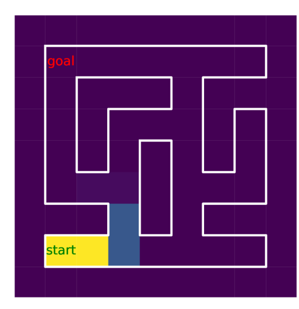
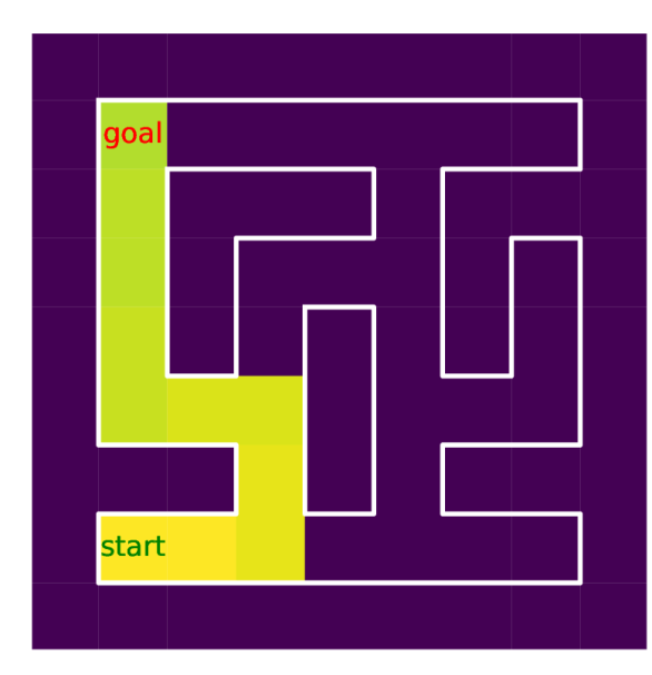
(a) optimal policy

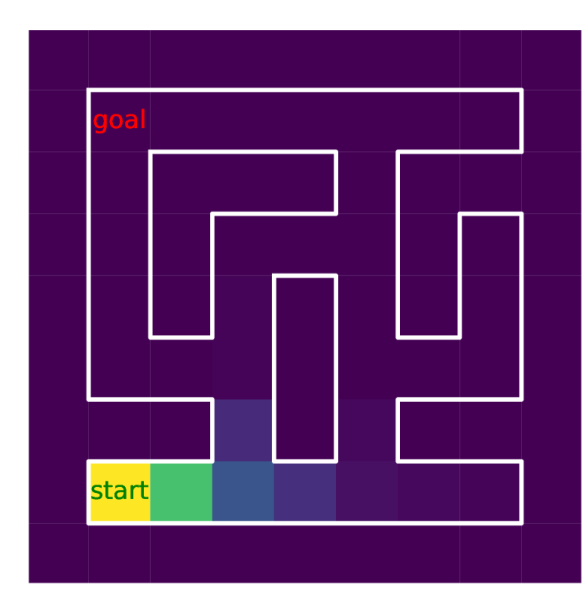
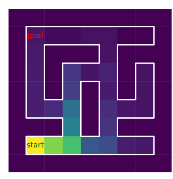
(b) CRUCB (Ours)

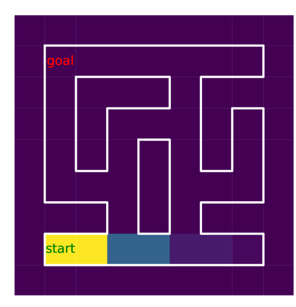
(c) R-ed-UCB

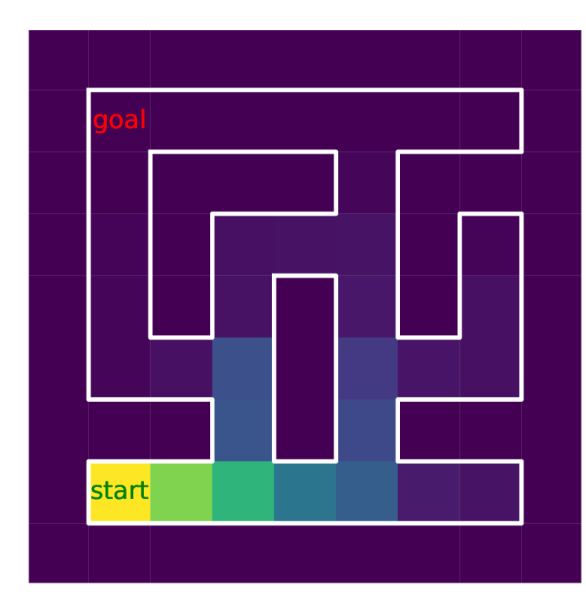
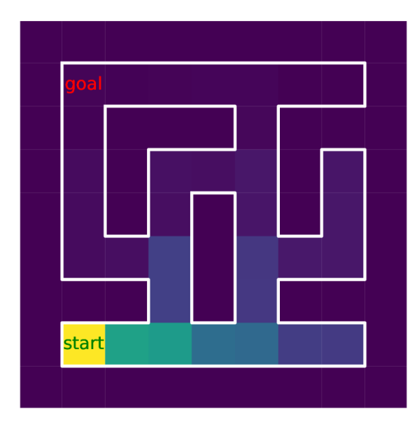
(d) SW-UCB

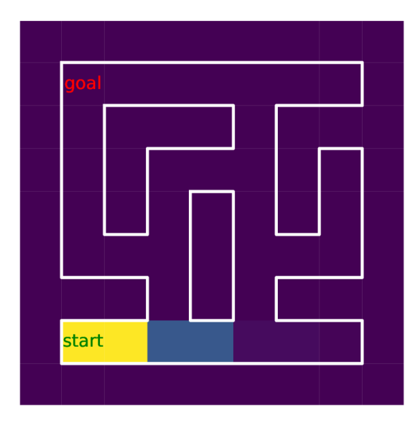
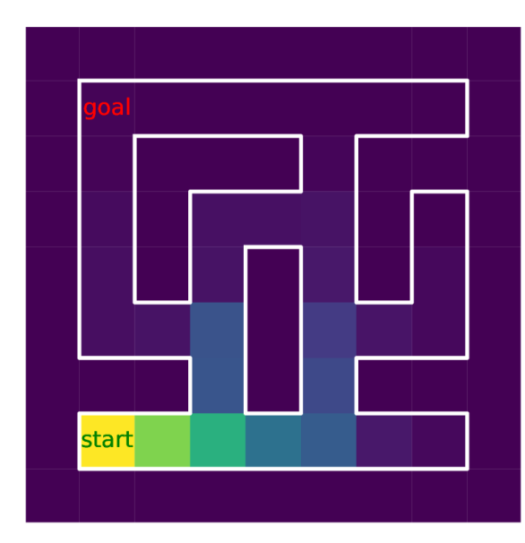
(e) SW-TS

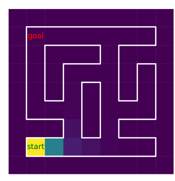
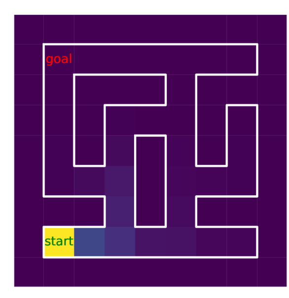
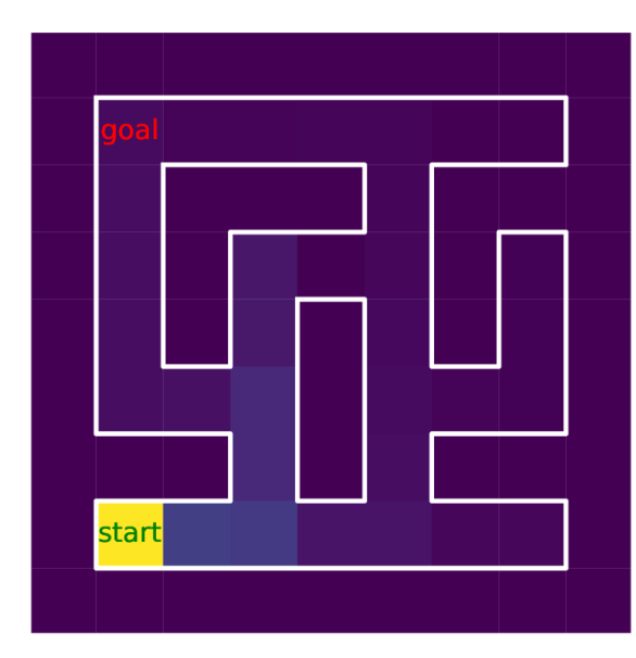
(f) SW-CUCB

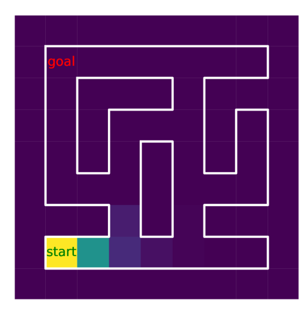
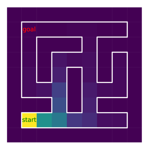
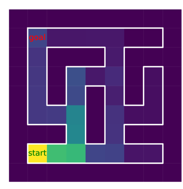
(g) SW-CTS

Figure 8: Heatmap illustrating visit frequencies in AntMaze-complex. We visualize the visit frequencies for the optimal policy, CRUCB, and baseline algorithms. The heatmap includes three rows representing visit frequencies until episode numbers 100, 500, and 3000.

In Figure 7, we only illustrate the performance of the optimal policy, CRUCB, and R-ed-UCB up to episode number 3000 due to space constraints. In Figure 8, we provide a more comprehensive view by illustrating the exploration patterns across all baseline algorithms at various stages. The optimal policy, which follows the oracle constant policy, only explores the optimal path from the start to the goal, resulting in highly focused exploration along this path, as depicted in Figure 8(a). In Figure 8(b), CRUCB exhibits exploration patterns most similar to the optimal policy compared to other baselines, demonstrating its efficiency in targeting the goal effectively. Among the baselines, SW-CTS notably aligns most closely with the optimal policy in the exploration patterns and is the only algorithm to show a significant difference in regret compared to the others, as seen in Figure 6(b). In comparison, algorithms not specifically designed for combinatorial settings, such as R-ed-UCB, SW-UCB, and SW-TS, suffer from less efficient exploration. Their exploration resembles a breadth-first search pattern, as they must explore a broader range of super arms despite having a given goal.

References

- Arora, Dekel, and Tewari (2012) Arora, R.; Dekel, O.; and Tewari, A. 2012. Online bandit learning against an adaptive adversary: from regret to policy regret. arXiv preprint arXiv:1206.6400.
- Auer et al. (2002) Auer, P.; Cesa-Bianchi, N.; Freund, Y.; and Schapire, R. E. 2002. The nonstochastic multiarmed bandit problem. SIAM journal on computing, 32(1): 48–77.
- Besbes, Gur, and Zeevi (2014) Besbes, O.; Gur, Y.; and Zeevi, A. 2014. Stochastic multi-armed-bandit problem with non-stationary rewards. Advances in neural information processing systems, 27.
- Cao et al. (2019) Cao, Y.; Wen, Z.; Kveton, B.; and Xie, Y. 2019. Nearly optimal adaptive procedure with change detection for piecewise-stationary bandit. In The 22nd International Conference on Artificial Intelligence and Statistics, 418–427. PMLR.
- Chen et al. (2020) Chen, W.; Du, Y.; Huang, L.; and Zhao, H. 2020. Combinatorial pure exploration for dueling bandit. In International Conference on Machine Learning, 1531–1541. PMLR.
- Chen, Du, and Kuroki (2020) Chen, W.; Du, Y.; and Kuroki, Y. 2020. Combinatorial pure exploration with partial or full-bandit linear feedback. arXiv preprint arXiv:2006.07905.
- Chen et al. (2016) Chen, W.; Hu, W.; Li, F.; Li, J.; Liu, Y.; and Lu, P. 2016. Combinatorial multi-armed bandit with general reward functions. Advances in Neural Information Processing Systems, 29.
- Chen et al. (2021) Chen, W.; Wang, L.; Zhao, H.; and Zheng, K. 2021. Combinatorial semi-bandit in the non-stationary environment. In Uncertainty in Artificial Intelligence, 865–875. PMLR.
- Chen, Wang, and Yuan (2013) Chen, W.; Wang, Y.; and Yuan, Y. 2013. Combinatorial Multi-Armed Bandit: General Framework and Applications. In Proceedings of the 30th International Conference on Machine Learning, 151–159. PMLR.
- Combes et al. (2015) Combes, R.; Talebi Mazraeh Shahi, M. S.; Proutiere, A.; and lelarge, m. 2015. Combinatorial Bandits Revisited. In Advances in Neural Information Processing Systems, volume 28, 2116–2124.
- Dijkstra (1959) Dijkstra, E. W. 1959. A note on two problems in connexion with graphs. Numerische Mathematik, 269–271.
- Edmonds (1965) Edmonds, J. 1965. Maximum matching and a polyhedron with 0, 1-vertices. Journal of research of the National Bureau of Standards B, 69(125-130): 55–56.
- Garivier and Moulines (2011) Garivier, A.; and Moulines, E. 2011. On upper-confidence bound policies for switching bandit problems. In International conference on algorithmic learning theory, 174–188. Springer.
- Heidari, Kearns, and Roth (2016) Heidari, H.; Kearns, M. J.; and Roth, A. 2016. Tight Policy Regret Bounds for Improving and Decaying Bandits. In IJCAI, 1562–1570.
- Kober, Bagnell, and Peters (2013) Kober, J.; Bagnell, J. A.; and Peters, J. 2013. Reinforcement learning in robotics: A survey. The International Journal of Robotics Research, 32(11): 1238–1274.
- Kruskal (1956) Kruskal, J. B. 1956. On the shortest spanning subtree of a graph and the traveling salesman problem. Proceedings of the American Mathematical society, 7(1): 48–50.
- Kveton et al. (2015a) Kveton, B.; Wen, Z.; Ashkan, A.; and Szepesvari, C. 2015a. Combinatorial cascading bandits. Advances in Neural Information Processing Systems, 28.
- Kveton et al. (2015b) Kveton, B.; Wen, Z.; Ashkan, A.; and Szepesvari, C. 2015b. Tight regret bounds for stochastic combinatorial semi-bandits. In Artificial Intelligence and Statistics, 535–543. PMLR.
- Lattimore and Szepesvári (2020) Lattimore, T.; and Szepesvári, C. 2020. Bandit algorithms. Cambridge University Press.
- Li et al. (2018) Li, L.; Jamieson, K.; DeSalvo, G.; Rostamizadeh, A.; and Talwalkar, A. 2018. Hyperband: A novel bandit-based approach to hyperparameter optimization. Journal of Machine Learning Research, 18(185): 1–52.
- Li et al. (2016) Li, S.; Wang, B.; Zhang, S.; and Chen, W. 2016. Contextual combinatorial cascading bandits. In International conference on machine learning, 1245–1253. PMLR.
- Metelli et al. (2022) Metelli, A. M.; Trovo, F.; Pirola, M.; and Restelli, M. 2022. Stochastic rising bandits. In International Conference on Machine Learning, 15421–15457. PMLR.
- Nourani-Koliji, Ghoorchian, and Maghsudi (2022) Nourani-Koliji, B.; Ghoorchian, S.; and Maghsudi, S. 2022. Linear combinatorial semi-bandit with causally related rewards. arXiv preprint arXiv:2212.12923.
- Talebi et al. (2017) Talebi, M. S.; Zou, Z.; Combes, R.; Proutiere, A.; and Johansson, M. 2017. Stochastic online shortest path routing: The value of feedback. IEEE Transactions on Automatic Control, 63(4): 915–930.
- Tekin and Liu (2012) Tekin, C.; and Liu, M. 2012. Online Learning of Rested and Restless Bandits. IEEE Transactions on Information Theory, 58: 5588–5611.
- Trovo et al. (2020) Trovo, F.; Paladino, S.; Restelli, M.; and Gatti, N. 2020. Sliding-window thompson sampling for non-stationary settings. Journal of Artificial Intelligence Research, 68: 311–364.
- Vezhnevets et al. (2017) Vezhnevets, A. S.; Osindero, S.; Schaul, T.; Heess, N.; Jaderberg, M.; Silver, D.; and Kavukcuoglu, K. 2017. Feudal networks for hierarchical reinforcement learning. In International Conference on Machine Learning, 3540–3549. PMLR.
- Wang and Chen (2018) Wang, S.; and Chen, W. 2018. Thompson sampling for combinatorial semi-bandits. In International Conference on Machine Learning, 5114–5122. PMLR.
- Wang, Chen, and Vojnović (2023) Wang, Y.; Chen, W.; and Vojnović, M. 2023. Combinatorial Bandits for Maximum Value Reward Function under Max Value-Index Feedback. arXiv preprint arXiv:2305.16074.
- Wei and Luo (2018) Wei, C.-Y.; and Luo, H. 2018. More adaptive algorithms for adversarial bandits. In Conference On Learning Theory, 1263–1291. PMLR.
- Wei and Srivatsva (2018) Wei, L.; and Srivatsva, V. 2018. On abruptly-changing and slowly-varying multiarmed bandit problems. In 2018 Annual American Control Conference (ACC), 6291–6296. IEEE.
- Wen et al. (2017) Wen, Z.; Kveton, B.; Valko, M.; and Vaswani, S. 2017. Online influence maximization under independent cascade model with semi-bandit feedback. Advances in neural information processing systems, 30.
- Wu et al. (2020) Wu, X.; Fu, L.; Zhang, Z.; Long, H.; Meng, J.; Wang, X.; and Chen, G. 2020. Evolving influence maximization in evolving networks. ACM Transactions on Internet Technology (TOIT), 20(4): 1–31.
- Xia et al. (2024) Xia, Y.; Kong, F.; Yu, T.; Guo, L.; Rossi, R. A.; Kim, S.; and Li, S. 2024. Which LLM to Play? Convergence-Aware Online Model Selection with Time-Increasing Bandits. In Proceedings of the ACM on Web Conference 2024, 4059–4070.
- Yoon et al. (2024) Yoon, Y.; Lee, G.; Ahn, S.; and Ok, J. 2024. Breadth-First Exploration on Adaptive Grid for Reinforcement Learning. In Forty-first International Conference on Machine Learning.