Gaussian quasi-likelihood analysis for non-Gaussian linear mixed-effects model with system noise

Abstract.

We consider statistical inference for a class of mixed-effects models with system noise described by a non-Gaussian integrated Ornstein-Uhlenbeck process. Under the asymptotics where the number of individuals goes to infinity with possibly unbalanced sampling frequency across individuals, we prove some theoretical properties of the Gaussian quasi-likelihood function, followed by the asymptotic normality and the tail-probability estimate of the associated estimator. In addition to the joint inference, we propose and investigate the three-stage inference strategy, revealing that they are first-order equivalent while quantitatively different in the second-order terms. Numerical experiments are given to illustrate the theoretical results.

1. Introduction

1.1. Background and motivation

This paper aims to develop a theory of statistical inference for a class of models used in analyses of longitudinal data. Longitudinal data are measurements or observations repeated over time for multiple individuals; for example, in HIV research, the CD4 lymphocyte count or the HIV viral load (so-called biomarkers) as response variables. These longitudinal data analyses aim to infer or evaluate changes in the mean structure of the response variable over time, the effects of covariates on the response variable, and the within-individual correlation of the response variable.

When planning to measure or collect longitudinal data, the time points at which the data will be measured are usually set in advance. However, due to reasons such as dropout from the longitudinal study, not all individuals are necessarily measured at all planned time points. In such cases, the number of measurements varies across individuals, and the time intervals between measurements within and between individuals differ; such a data set is called “unbalanced”. As a traditional approach to handling unbalanced data, the linear mixed-effects models [9] are frequently used to analyze a continuous response variable in the unbalanced longitudinal dataset. As an alternative approach, linear mixed-effects models with a Gaussian integrated Ornstein-Uhlenbeck (OU) process as a system noise are proposed in [17]; see also [5]. A special feature of this model is that we could estimate a degree of derivative tracking from longitudinal data [2]. Suppose each individual’s trajectory tends to shift on a linear path. In that case, the model is said to have a strong derivative tracking (i.e., linear mixed-effects model in which explanatory variables for fixed and random effects include time variables). On the other hand, if the slope of each individual’s trajectory tends to continually change, the model is said to have weak derivative tracking. See [17] for more detail on the derivative tracking.

The previous study [6] has shown the local asymptotics normality and the optimality of a local maximum-likelihood estimator for a class of Gaussian linear mixed-effects models having the integrated OU processes as system noises. Although the classical linear mixed-effects models are usually applied under the Gaussianity of the random effect and the measurement error, there have been some studies about model misspecification of the random effect in the context of (generalized) linear mixed-effects models, e.g. [14] and [15].

In this paper, we consider a class of linear mixed-effects models having the possibly non-Gaussian integrated Lévy-driven OU process as system noise. On the one hand, as in [17], thanks to the continuous-time framework, this framework allows us to smoothly handle an unbalanced longitudinal data set in a unified manner; this nice feature cannot hold for the discrete-time first-order autoregressive structure. On the other hand, by adding the integrated OU process term, the Gaussian quasi-likelihood function becomes nonlinear with respect to the parameter associated with the OU process, raising concern about the large computational load of simultaneous optimizations for parameter estimates [6]. To mitigate this problem, we propose a three-stage stepwise inference strategy in which the mean and covariance structures are optimized separately and alternately. By splitting the target parameters, the computational load is reduced compared to the simultaneous optimization.

In our main result, we will show the very strong mode of convergence of the quasi-likelihood-ratio random field, namely, not only the weak convergence (locally asymptotically quadratic property) and uniform tail-probability estimate. To the best of our knowledge, within the class of linear mixed-effects models, there has been no previous study that compared joint likelihood inference with stepwise likelihood inference in terms of computational load and theoretical properties.

1.2. Setup and objective

Suppose that we are given a longitudinal data set from $i$th individual at given time points $0=t_{i0}<t_{i1}<\dots<t_{in_{i}}$, described by

$$Y_{i}(t_{ij}) =X_{i}(t_{ij})^{\top}\beta+Z_{i}(t_{ij})^{\top}b_{i}+W_{i}(t_{ij})+\epsilon_{i}(t_{ij})$$ (1.1)

for $1\leq i\leq N$ and $1\leq j\leq n_{i}$, where $\top$ denotes the transposition of a matrix and

$$\max_{i\leq N}n_{i}=O(1).$$ (1.2)

Here and in what follows, the asymptotics is taken for $N\to\infty$. We will use the generic convention $\xi_{ij}=\xi_{i}(t_{ij})$, so that (1.1) becomes

$$Y_{ij}=X_{ij}^{\top}\beta+Z_{ij}^{\top}b_{i}+W_{ij}+\epsilon_{ij}.$$ (1.3)

The ingredients are specified as follows.

• $X_{ij}\in\mathbb{R}^{p_{\beta}}$ and $Z_{ij}\in\mathbb{R}^{p_{b}}$ denote non-random explanatory variables for fixed and random effects of the $i$th individual, respectively, such that

  $$\sup_{N}\max_{i\leq N}\left(|X_{i}|+|Z_{i}|\right)<\infty,$$

  where, with a slight abuse of notation, $X_{i}:=(X_{ij})_{j=1}^{n_{i}}\in\mathbb{R}^{n_{i}}\otimes\mathbb{R}^{p_{\beta}}$ and $Z_{i}:=(Z_{ij})_{j=1}^{n_{i}}\in\mathbb{R}^{n_{i}}\otimes\mathbb{R}^{p_{b}}$, and $|\cdot|$ denotes the Euclidean norm.

• $\beta\in\mathbb{R}^{p_{\beta}}$ is the unknown fixed-effect parameter, which is common across the individuals.

• Let $b_{1},b_{2},\dots$ denote unobserved random-effect which are i.i.d. zero-mean random variables in $\mathbb{R}^{p_{b}}$ with common nonnegative-definite covariance matrix $\Psi(\gamma)$ for some function $\Psi:\,\mathbb{R}^{\gamma}\to\mathbb{R}^{p_{b}}\otimes\mathbb{R}^{p_{b}}$.

  • We do not fully specify the common distribution $\mathcal{L}(b_{1})$. For a specific form of $\Psi(\gamma)$, one may adopt the unstructured setting where all the entries of $\Psi(\gamma)$ are fully unknown. However, it may suffer from computational issues caused by the high dimensionality of the parameters.

• The stochastic processes $W_{i}(\cdot)$ represents unobserved random system-noise processes driving the $i$th individual ($i=1,\dots,N$), described as the integrated Ornstein-Uhlenbeck (intOU) process:

  $$W_{i}(t)=\int_{0}^{t}\zeta_{i}(s)ds,$$

  where $\zeta_{i}(\cdot)$ denotes the Lévy-driven OU process with the autoregression parameter $\lambda>0$ and the scale coefficient $\sigma>0$; see (1.4) below.

• The processes $\epsilon_{1}(\cdot),\epsilon_{2}(\cdot),\dots$ denote i.i.d. white noise process representing measurement error: for each $i$, the variables $\epsilon_{i}(t_{i1}),\dots,\epsilon_{i}(t_{in_{i}})$ are centered and uncorrelated, and have variance $\sigma_{\epsilon}^{2}$.

• The random variables $\{b_{i}\}$, $\{W_{i}(\cdot)\}$, and $\{\epsilon_{i}\}$ are mutually independent.

All the random elements introduced above are defined on an underlying filtered probability space endowed with the i.i.d. random sequence

$$\{(b_{i},\zeta_{i}(0),(L_{i}(t))_{t\leq T},(\epsilon_{i}(t_{ij}))_{j\leq n_{i}})\}_{i\geq 1},$$

where $T>0$ is a fixed number for which $\sup_{N\geq 1}\max_{i\leq N}\max_{j\leq n_{i}}t_{ij}\leq T$ (such a $T$ does exist under (1.2)). As before, we will simply write the response-variable vectors $Y_{i}:=(Y_{ij})_{j=1}^{n_{i}}\in\mathbb{R}^{n_{i}}$, $1\leq i\leq N$, so that

$$Y_{i}=X_{i}\beta+Z_{i}b_{i}+W_{i}+\epsilon_{i}$$

in the matrix-product form.

The model for the observation $\{(X_{i},Y_{i},Z_{i})\}_{i\leq N}$ is thus indexed by the finite-dimensional parameter

$$\theta:=(\beta,v)=\left(\beta,\gamma,\lambda,\sigma^{2},\sigma_{\epsilon}^{2}\right)\in\Theta =\Theta_{\beta}\times\Theta_{v}=\Theta_{\beta}\times\Theta_{\gamma}\times\Theta_{\lambda}\times\Theta_{\sigma^{2}}\times\Theta_{\sigma_{\epsilon}^{2}}$$

$$\subset\mathbb{R}^{p_{\beta}}\times\mathbb{R}^{p_{\gamma}}\times(0,\infty)\times(0,\infty)\times(0,\infty)$$

with $v:=(\gamma,\lambda,\sigma^{2},\sigma_{\epsilon}^{2})$ denoting the covariance parameter. We assume that the parameter space $\Theta$ is a bounded convex domain in $\mathbb{R}^{p}$ with $p:=p_{\beta}+p_{v}$, where $p_{v}:=p_{\gamma}+3$ denotes the dimension of $v$. Throughout, we fix a point $\theta_{0}=(\beta_{0},v_{0})\in\Theta$ as true value of $\theta$, assumed to exist. It should be noted that the parameter may not completely characterize the distribution of the model, for we do not fully specify the distributions of $b_{i}$ and $\zeta_{i}$; in this sense, the model is semiparametric. We will denote by $P_{\theta}$, $E_{\theta}$, $\mathrm{Var}_{\theta}$, and $\mathrm{Cov}_{\theta}$ for the corresponding probability, expectation, variance, and covariance, respectively. The subscript “$\theta_{0}$” will be omitted such as $P=P_{\theta_{0}}$ and $E=E_{\theta_{0}}$.

For convenience, we briefly mention some preliminary facts about the intOU process $W_{i}(\cdot)$. Let $\zeta_{1}(\cdot),\zeta_{2}(\cdot),\dots$ be i.i.d. OU processes given by the stochastic differential equation

$$d\zeta_{i}(t)=-\lambda\zeta_{i}(t)dt+\sigma dL_{i}(t)$$ (1.4)

for $i=1,\dots,N$, where $L_{1},L_{2},\dots$ are i.i.d. càdlàg Lévy processes such that $E_{\theta}[L_{i}(t)]=0$ and $\mathrm{Var}_{\theta}[L_{i}(t)]=t$ for $t\in[0,T]$. The process $\zeta_{i}$ has a unique invariant distribution. We assume that $\zeta_{i}$ are strictly stationary, that is, $\zeta_{i}(0)$ obeys the invariant distribution; in this case, we can write

$$\zeta_{i}(t)=\int_{-\infty}^{t}e^{-\lambda(t-s)}\sigma dL_{i}(s)$$

for a two-sided version $(L_{i}(t))_{t\in\mathbb{R}}$ of $L_{i}$. We know that each $\zeta_{i}$ is exponentially ergodic. We refer to [11], [12], and the references therein for related details. Now, we define $W_{i}(t)$ as unobserved random system-noise processes driving the $i$th individual ($i=1,\dots,N$), described as the integrated-Ornstein-Uhlenbeck (intOU) process:

$$W_{i}(t) :=\int_{0}^{t}\zeta_{i}(s)ds$$

$$=\int_{0}^{t}\left(e^{-\lambda s}\zeta_{i}(0)+\sigma\int_{0}^{s}e^{-\lambda(s-v)}dL_{i}(v)\right)ds$$

$$=\frac{\zeta_{i}(0)}{\lambda}(1-e^{-\lambda t})+\frac{\sigma}{\lambda}\int_{0}^{t}(1-e^{-\lambda(t-v)})dL_{i}(v).$$

We denote by $H_{i}(\lambda,\sigma^{2})=(H_{i;jk}(\lambda,\sigma^{2}))_{j,k=1}^{n_{i}}\in\mathbb{R}^{n_{i}}\otimes\mathbb{R}^{n_{i}}$ the covariance matrix of $W_{i}:=(W_{ij})_{j=1}^{n_{i}}$:

$$H_{i;jk}(\lambda,\sigma^{2}) :=\mathrm{Cov}_{\theta}\left[W_{ij},W_{ik}\right]$$

$$=\frac{\sigma^{2}}{2\lambda^{3}}\left(2\lambda\min(t_{ij},t_{ik})+e^{-\lambda t_{ij}}+e^{-\lambda t_{ik}}-1-e^{-\lambda|t_{ij}-t_{ik}|}\right).$$ (1.5)

Under the aforementioned setup, our objective in this paper is to investigate the asymptotic behavior of the marginal Gaussian quasi-likelihood (GQLF) random functions, based on which we can prove the asymptotic normality, the second-order asymptotic expansion, and the tail-probability estimate of the associated estimator. The GQLF provides us with an explicit inference strategy only by using the second-order (covariance) structure without full distributional specification of the underlying model. We will formulate the two kinds of the GQLF, the joint and the stepwise ones. Although our primary interest is the intOU mixed-effects model (1.3), in the main sections 2 and 3 we will work with the following notation for the mean vector and the covariance matrix:

$$\mu_{i}(\beta) :=E_{\theta}[Y_{i}]=X_{i}\beta,$$

$$\Sigma_{i}(v) :=\mathrm{Cov}_{\theta}[Y_{i}]=Z_{i}\Psi(\gamma)Z_{i}^{\top}+H_{i}(\lambda,\sigma^{2})+\sigma_{\epsilon}^{2}I_{n_{i}}.$$ (1.6)

This will not only make the arguments more convenient and transparent but also extensions to various non-linear settings straightforward.

1.3. Outline

We first study the joint GQLF in Section 2 and then the stepwise GQLF in Section 3. In both cases, we obtain the asymptotic normality, the second-order stochastic expansion of the estimator, and the tail-probability estimate. Section 4 provides some remarks about the original setup (1.3). Section 5 presents some illustrative simulation results.

1.4. Basic notation

For two real positive sequences $(a_{N})$ and $(b_{N})$, we write $a_{N}\lesssim b_{N}$ if $\limsup_{N}(a_{N}/b_{N})<\infty$. We use the multilinear-form notation

$$M[u_{i_{1}},\dots,u_{i_{m}}]:=\sum_{i_{1}\dots i_{m}}M_{i_{1}\dots i_{m}}u_{i_{1}}\dots u_{i_{m}}$$

for a tensor $M=\{M_{i_{1}\dots i_{m}}\}$; it may take values in a multilinear form. For a square matrix $A$, we denote its Frobenius norm by $|A|$, minimum eigenvalue by $\lambda_{\min}(A)$, and trace by $\mathop{\rm Tr}(A)$. The $d$-dimensional identity matrix is denoted by $I_{d}$. The $k$th partial differentiation operator with respect to variables $a$ is denoted by $\partial^{k}_{a}$, with $\partial_{a}$ for $k=1$. We use the symbol $\phi_{n_{i}}(\cdot;\mu,\Sigma)$ for the $n_{i}$-dimensional Gaussian $N_{n_{i}}(\mu,\Sigma)$-density.

1.5. Comments on model selection

Our results include the asymptotic normality at rate $\sqrt{N}$ of the form $\sqrt{N}(\hat{\theta}_{N}-\theta_{0})\xrightarrow{\mathcal{L}}N_{p}\left(0,\,\Gamma_{0}^{-1}S_{0}\Gamma_{0}^{-1}\right)$ and the tail-probability estimate $\sup_{N}P[|\sqrt{N}(\hat{\theta}_{N}-\theta_{0})|>r]\lesssim r^{-L}$ for any $L>0$. With these results, it is routine to derive the fundamental model selection criteria: the classical marginal Akaike information criteria (AIC) and also Schwarz’s Bayesian information criterion (BIC), related to the joint GQLF $\mathbb{H}_{N}(\theta)$: we obtain the forms:

$$-2\mathbb{H}_{N}(\hat{\theta}_{N})+2\mathop{\rm Tr}(\hat{\Gamma}_{N}^{\prime-1}\hat{S}^{\prime}_{N})$$

for AIC, where $\hat{\Gamma}^{\prime}_{N}$ and $\hat{S}^{\prime}_{N}$ are suitable consistent estimators of $\Gamma_{0}$ and $S_{0}$, respectively, and

$$-2\mathbb{H}_{N}(\hat{\theta}_{N})+p\log N$$

for BIC. Concerning this point, we refer to [3] and [4] for detailed studies of AIC- and BIC-type statistics based on the GQLF.

Yet another well-known information criterion is the conditional AIC (cAIC) introduced in [18]; see also [8] and [16] for some details of a conditional AIC based on the genuine likelihood. Formulation and derivation of the cAIC will require some different considerations, and we hope to report it elsewhere.

2. Joint Gaussian quasi-likelihood analysis

The joint GQLF is defined by

$$\mathbb{H}_{N}(\theta)=\mathbb{H}_{N}(\beta,v):=\sum_{i=1}^{N}\log\phi_{n_{i}}\left(Y_{i};\,\mu_{i}(\beta),\Sigma_{i}(v)\right).$$

Although the data generating distribution $\mathcal{L}(Y_{i})$ may not be Gaussian, we set our statistical model Gaussian with possibly different dimensions across the indices $i=1,\dots,N$; of course, $\mathbb{H}_{N}(\theta)$ is the exact log-likelihood if $Y_{1},\dots,Y_{N}$ are truly Gaussian.

In addition to the standing assumptions described in Section 1.2, we impose further regularity conditions. Denote by $\overline{\Theta}$ the closure of $\Theta$.

Assumption 2.1.

1. The functions $\theta\mapsto(\mu_{i}(\beta),\Sigma_{i}(v))$ $(i\geq 1)$ are of class $\mathcal{C}^{4}(\Theta)$ and all the derivatives with itself are continuous in $\theta\in\overline{\Theta}$.

2. $\displaystyle{\inf_{N}\min_{1\leq i\leq N}\inf_{v\in\Theta_{v}}\lambda_{\min}(\Sigma_{i}(v))>0}$.

3. $\displaystyle{\sup_{N\geq 1}\max_{1\leq i\leq N}\max_{1\leq k\leq 4}\left(\sup_{\beta\in\Theta_{\beta}}|\partial_{\beta}^{k}\mu_{i}(\beta)|\vee\sup_{v\in\Theta_{v}}|\partial_{v}^{k}\Sigma_{i}(v)|\right)<\infty}$.

Assumption 2.2.

$E[|L_{1}(t)|^{q}]+E[|\epsilon_{1}(t)|^{q}]+E[|b_{1}|^{q}]<\infty$ for every $q>0$ and $t\leq T$.

The joint Gaussian quasi-maximum likelihood estimator (GQMLE) is defined to be any element

$$\hat{\theta}_{N}=(\hat{\beta}_{N},\hat{v}_{N})\in\mathop{\rm argmax}_{\theta\in\overline{\Theta}}\mathbb{H}_{N}(\theta).$$

Under Assumption 2.2, at least one such $\hat{\theta}_{N}$ does exist ($P$-)a.s.

2.1. Uniform convergence of quasi-Kullback-Leibler divergence

To deduce the consistency of the joint GQMLE, we will prove the asymptotic behavior of the normalized quasi-Kullback-Leibler divergence associated with $\mathbb{H}_{N}$, defined by

$$\mathbb{Y}_{N}(\theta):=\frac{1}{N}\left(\mathbb{H}_{N}(\theta)-\mathbb{H}_{N}(\theta_{0})\right).$$

Let us write $\mathbb{Y}_{N}(\theta)=N^{-1}\sum_{i=1}^{N}\xi_{i}(\theta)$, where

$$\xi_{i}(\theta) :=\frac{1}{2}\Big{(}\log|\Sigma_{i}(v_{0})|-\log|\Sigma_{i}(v)|-\Sigma_{i}(v)^{-1}[(\mu_{i}(\beta_{0})-\mu_{i}(\beta))^{\otimes 2}]$$

$${}\qquad+(\Sigma_{i}(v_{0})^{-1}-\Sigma_{i}(v)^{-1})[(Y_{i}-\mu_{i}(\beta_{0}))^{\otimes 2}]$$

$${}\qquad-2\Sigma_{i}(v)^{-1}[\mu_{i}(\beta_{0})-\mu_{i}(\beta),Y_{i}-\mu_{i}(\beta_{0})]\Big{)}.$$

For each $\theta$,

$$E[\xi_{i}(\theta)] =\frac{1}{2}\Big{(}\log|\Sigma_{i}(v_{0})|-\log|\Sigma_{i}(v)|-\mathop{\rm Tr}\left(\Sigma_{i}(v)^{-1}\Sigma_{i}(v_{0})-I_{n_{i}}\right)$$

$$\qquad-\Sigma_{i}(v)^{-1}[(\mu_{i}(\beta)-\mu_{i}(\beta_{0}))^{\otimes 2}]\Big{)}.$$

Let

$$F_{N,1}(v) :=\frac{1}{N}\sum_{i=1}^{N}\{\log|\Sigma_{i}(v_{0})|-\log|\Sigma_{i}(v)|-\mathop{\rm Tr}\left(\Sigma_{i}(v)^{-1}\Sigma_{i}(v_{0})-I_{n_{i}}\right)\},$$

$$F_{N,2}(\theta) :=\frac{1}{N}\sum_{i=1}^{N}\Sigma_{i}(v)^{-1}[(\mu_{i}(\beta)-\mu_{i}(\beta_{0}))^{\otimes 2}].$$

Note that we are not assuming any structural assumptions on the sequences $(X_{ij})$ and $(Z_{ij})$. To ensure the convergence of $\mathbb{Y}_{N}(\cdot)$ to a specific limit in probability, we impose the following.

Assumption 2.3.

There exist non-random $\mathcal{C}^{2}(\Theta)$-functions $F_{0,1}(v)=F_{0,1}(v;v_{0})$ and $F_{0,2}(\theta)=F_{0,2}(\theta;\beta_{0})$ such that

$$\sup_{N}\sup_{\theta}\left(\sqrt{N}|F_{N,1}(v)-F_{0,1}(v)|+\sqrt{N}|F_{N,2}(\theta)-F_{0,2}(\theta)|\right)<\infty.$$

and that $F_{0,1}(v)$ and $F_{0,2}(\theta)$ and their partial derivatives of orders $\leq 2$ are continuous in $\overline{\Theta}$.

Remark 2.4.

In our setting, the explicit forms of $F_{0,1}(v)$ and $F_{0,2}(\theta)$ are not available in general because of the possible unbalanced nature of the longitudinal data under consideration; unfortunately, it is the case even when we assume that $(X_{i},Z_{i})$ is the sequence of i.i.d. random processes. Concerned with the identification of the limits, we have the same situations in Assumptions 2.7 and 2.8 below. Still, the situation could be simplified to some extent when $\mu_{i}(\beta)=X_{i}\beta$. See Section 4.

Assumption 2.3 implies that

$$\sup_{N}\sup_{\theta\in\Theta}\left|\sqrt{N}\left(\frac{1}{N}\sum_{i=1}^{N}E[\xi_{i}(\theta)]-\mathbb{Y}_{0}(\theta)\right)\right|<\infty,$$ (2.1)

where

$$\mathbb{Y}_{0}(\theta):=\frac{1}{2}\left(F_{0,1}(v)-F_{0,2}(\theta)\right)$$ (2.2)

is a non-random $\mathcal{C}^{2}(\Theta)$-function. We see that $F_{0,1}(v)\leq 0$ by invoking the property of the Kullback-Leibler divergence between two multivariate normal distributions. Since $F_{0,2}(\theta)\geq 0$, it holds that $\mathbb{Y}_{0}(\theta)\leq 0$. We follow the custom of [19] to state the identifiability condition:

Assumption 2.5.

There exists a constant $\chi_{0}>0$ such that $F_{0,1}(v)\leq-\chi_{0}|v-v_{0}|^{2}$ and $F_{0,2}(\theta)\geq\chi_{0}|\theta-\theta_{0}|^{2}$ for every $\theta\in\Theta$.

The following two conditions are sufficient for Assumption 2.5:

• $\{\theta_{0}\}=\mathop{\rm argmax}_{\theta\in\overline{\Theta}}\mathbb{Y}_{0}(\theta)$, namely, $\mathbb{Y}_{0}(\theta)=0$ if and only if $\theta=\theta_{0}$;

• $-\partial_{\theta}^{2}\mathbb{Y}_{0}(\theta_{0})$ is positive definite.

The sufficiency can be seen through the Taylor expansion and the compactness of $\overline{\Theta}$: first, take $\delta>0$ small enough to ensure that

$$\sup_{\theta:\,|\theta-\theta_{0}|\leq\delta}|\theta-\theta_{0}|^{-2}\mathbb{Y}_{0}(\theta)\lesssim-\inf_{\tilde{\theta}:\,|\tilde{\theta}-\theta_{0}|\leq\delta}(-\partial_{\theta}^{2}\mathbb{Y}_{0}(\tilde{\theta}))\leq-\chi_{0,1}$$

for some $\chi_{0,1}<0$; second, with the so chosen $\delta>0$, the compactness implies that

$$\sup_{\theta:\,|\theta-\theta_{0}|>\delta}|\theta-\theta_{0}|^{-2}\mathbb{Y}_{0}(\theta)\leq\delta^{-2}\sup_{\theta:\,|\theta-\theta_{0}|>\delta}\mathbb{Y}_{0}(\theta)\leq-\chi_{0,2}$$

for some $\chi_{0,2}<0$. Hence Assumption 2.5 is verified with $\chi_{0}=\chi_{0,1}+\chi_{0,2}>0$.

Under Assumption 2.5, the consistency $\hat{\theta}_{N}\xrightarrow{p}\theta_{0}$ follows from the uniform convergences in probability $\sup_{\theta}|\mathbb{Y}_{N}(\theta)-\mathbb{Y}_{0}(\theta)|\xrightarrow{p}0$. We will derive it in the following stronger form:

$$\forall K>0,\quad\sup_{N}E\left[\sup_{\theta}\left(\sqrt{N}|\mathbb{Y}_{N}(\theta)-\mathbb{Y}_{0}(\theta)|\right)^{K}\right]<\infty.$$ (2.3)

Observe that

$$\mathbb{Y}_{N}(\theta)-\mathbb{Y}_{0}(\theta)=\frac{1}{N}\sum_{i=1}^{N}\left(\xi_{i}(\theta)-E[\xi_{i}(\theta)]\right)+\frac{1}{N}\sum_{i=1}^{N}E[\xi_{i}(\theta)]-\mathbb{Y}_{0}(\theta).$$

By (2.1), for (2.3) it remains to look at the first term on the right-hand side. We will make use of the following basic uniform moment estimates. Recall that $p$ denotes the dimension of $\theta$.

Lemma 2.6.

Let $\Theta\subset\mathbb{R}^{p}$ be a bounded convex domain, $q>p\vee 2$, and let $\chi_{Ni}(\theta):\Theta\to\mathbb{R}$, $i\leq N$, $N\geq 1$, be random functions. Then, we have

$$E\left[\sup_{\theta}\left|\sum_{i=1}^{N}\chi_{Ni}(\theta)\right|^{q}\right]\lesssim\sup_{\theta}E\left[\left|\sum_{i=1}^{N}\chi_{Ni}(\theta)\right|^{q}\right]+\sup_{\theta}E\left[\left|\sum_{i=1}^{N}\partial_{\theta}\chi_{Ni}(\theta)\right|^{q}\right]$$

If in particular $\partial_{\theta}^{k}\chi_{N1}(\theta),\dots,\partial_{\theta}^{k}\chi_{NN}(\theta)$ for $k\in\{0,1\}$ and $\theta\in\Theta$ forms a martingale difference array with respect to some filtration $(\mathcal{F}_{Ni})_{i\leq N}$, then

$$E\left[\sup_{\theta}\left|\frac{1}{\sqrt{N}}\sum_{i=1}^{N}\chi_{i}(\theta)\right|^{q}\right]\lesssim\sup_{\theta}\frac{1}{N}\sum_{i=1}^{N}E\left[|\chi_{i}(\theta)|^{q}\right]+\sup_{\theta}\frac{1}{N}\sum_{i=1}^{N}E\left[|\partial_{\theta}\chi_{i}(\theta)|^{q}\right].$$

Proof.

The first inequality is due to the Sobolev inequality [1] which says that $\sup_{\theta}|f(\theta)|\lesssim\int_{\Theta}(|f(\theta)|+|\partial_{\theta}f(\theta)|)d\theta$. Then, we can apply the Burkholder inequality to obtain the second one. ∎

Returning to our model setup, by Lemma 2.6 we have

$$E\left[\sup_{\theta\in\Theta}\left|\frac{1}{\sqrt{N}}\sum_{i=1}^{N}\left(\xi_{i}(\theta)-E[\xi_{i}(\theta)]\right)\right|^{K}\right]$$

$$\lesssim\sup_{\theta\in\Theta}E\left[\left|\frac{1}{\sqrt{N}}\sum_{i=1}^{N}\left(\xi_{i}(\theta)-E[\xi_{i}(\theta)]\right)\right|^{K}\right]$$

$$\qquad+\sup_{\theta\in\Theta}E\left[\left|\frac{1}{\sqrt{N}}\sum_{i=1}^{N}\left(\partial_{\theta}\xi_{i}(\theta)-E[\partial_{\theta}\xi_{i}(\theta)]\right)\right|^{K}\right].$$

From Burkholder’s inequality and Jensen’s equality, it follows that

$$E\left[\left|\frac{1}{\sqrt{N}}\sum_{i=1}^{N}\left(\xi_{i}(\theta)-E[\xi_{i}(\theta)]\right)\right|^{K}\right] \lesssim E\left[\left(\frac{1}{N}\sum_{i=1}^{N}\left|\xi_{i}(\theta)-E[\xi_{i}(\theta)]\right|^{2}\right)^{K/2}\right]$$

$$\leq\frac{1}{N}\sum_{i=1}^{N}E\left[\left|\xi_{i}(\theta)-E[\xi_{i}(\theta)]\right|^{K}\right].$$

For every $K>0$, we have

$$\sup_{N\geq 1}\max_{1\leq i\leq N}E[|Y_{i}|^{K}]<\infty$$ (2.4)

hence also $\sup_{N\geq 1}\max_{1\leq i\leq N}\sup_{\theta}E[|\xi_{i}(\theta)|^{K}]<\infty$. Therefore,

$$\sup_{N}\sup_{\theta\in\Theta}E\left[\left|\frac{1}{\sqrt{N}}\sum_{i=1}^{N}\left(\xi_{i}(\theta)-E[\xi_{i}(\theta)]\right)\right|^{K}\right]<\infty.$$

Similarly, we obtain

$$\sup_{N}\sup_{\theta\in\Theta}E\left[\left|\frac{1}{\sqrt{N}}\sum_{i=1}^{N}\left(\partial_{\theta}\xi_{i}(\theta)-E[\partial_{\theta}\xi_{i}(\theta)]\right)\right|^{K}\right]<\infty.$$

This concludes (2.3), hence the consistency $\hat{\theta}_{N}\xrightarrow{p}\theta_{0}$.

2.2. Quasi-score function

Define the quasi-score function by

$$\Delta_{N}(\theta)=\frac{1}{\sqrt{N}}\partial_{\theta}\mathbb{H}_{N}(\theta).$$

We have $\Delta_{N}(\theta)=(\Delta_{N,\beta}(\theta),\,\Delta_{N,v}(\theta))\in\mathbb{R}^{p_{\beta}}\times\mathbb{R}^{p_{v}}$ with

$$\Delta_{N,\beta}(\theta) :=\frac{1}{\sqrt{N}}\sum_{i=1}^{N}\Sigma_{i}(v)^{-1}[\partial_{\beta}\mu_{i}(\beta),Y_{i}-\mu_{i}(\beta)],$$ (2.5)

$$\Delta_{N,v}(\theta) :=\frac{1}{\sqrt{N}}\sum_{i=1}^{N}\bigg{(}\frac{1}{2}(\Sigma_{i}(v)^{-1}(\partial_{v_{j}}\Sigma_{i}(v))\Sigma_{i}(v)^{-1})[(Y_{i}-\mu_{i}(\beta))^{\otimes 2}]$$

$${}\qquad-\frac{1}{2}\mathop{\rm Tr}(\Sigma_{i}(v)^{-1}(\partial_{v_{j}}\Sigma_{i}(v)))\bigg{)}_{j=1}^{p_{v}}.$$ (2.6)

From now on, we will often omit “$(\theta_{0})$”, “$(\beta_{0})$”, and “$(v_{0})$” from the notation, such as $\Delta_{N}=\Delta_{N}(\theta_{0})$. Obviously, $E[\Delta_{N,\beta}]=E[\Delta_{N,v}]=0$. Let

$$A_{ij}:=\Sigma_{i}^{-1}(\partial_{v_{j}}\Sigma_{i})\Sigma_{i}^{-1}.$$ (2.7)

Then, the covariance matrix

$$S_{N}:=\mathrm{Cov}[\Delta_{N}]=\begin{pmatrix}\mathrm{Cov}[\Delta_{N,\beta}]&\mathrm{Cov}[\Delta_{N,\beta},\Delta_{N,v}]\\ \mathrm{Cov}[\Delta_{N,\beta},\Delta_{N,v}]^{\top}&\mathrm{Cov}[\Delta_{N,v}]\end{pmatrix}=:\begin{pmatrix}S_{N,11}&S_{N,12}\\ S_{N,12}^{\top}&S_{N,22}\end{pmatrix}$$

is given by

$$S_{N,11} =\frac{1}{N}\sum_{i=1}^{N}\Sigma_{i}^{-1}[(\partial_{\beta}\mu_{i})^{\otimes 2}]\in\mathbb{R}^{p_{\beta}}\otimes\mathbb{R}^{p_{\beta}},$$

$$S_{N,12} =\frac{1}{2N}\sum_{i=1}^{N}\left(\Sigma_{i}^{-1}[\partial_{\beta}\mu_{i},E[(Y_{i}-\mu_{i})^{\otimes 2}A_{ij}(Y_{i}-\mu_{i})]]\right)_{j=1}^{p_{v}}\in\mathbb{R}^{p_{\beta}}\otimes\mathbb{R}^{p_{v}},$$

$$S_{N,22} =\frac{1}{4N}\sum_{i=1}^{N}\bigg{(}E[\mathop{\rm Tr}(A_{ij}(Y_{i}-\mu_{i}^{\otimes 2})\cdot\mathop{\rm Tr}(A_{ik}(Y_{i}-\mu_{i})^{\otimes 2})]$$

$${}\qquad-\mathop{\rm Tr}\left(\Sigma_{i}^{-1}\partial_{v_{j}}\Sigma_{i}\right)\cdot\mathop{\rm Tr}\left(\Sigma_{i}^{-1}\partial_{v_{k}}\Sigma_{i}\right)\bigg{)}_{j,k=1}^{p_{v}}\in\mathbb{R}^{p_{v}}\otimes\mathbb{R}^{p_{v}}.$$

To identify the asymptotic covariance of $\Delta_{N}$, we need the convergence of $S_{N}$.

Assumption 2.7.

There exists a positive definite matrix

$$S_{0}=\begin{pmatrix}S_{0,11}&S_{0,12}\\ S_{0,12}^{\top}&S_{0,22}\end{pmatrix}\in\mathbb{R}^{p}\otimes\mathbb{R}^{p}$$

such that $(S_{N,11},S_{N,12},S_{N,22})\rightarrow(S_{0,11},S_{0,12},S_{0,22})$, hence $S_{N}\rightarrow S_{0}$, as $N\rightarrow\infty$.

Let $\Delta_{N}=:\sum_{i=1}^{N}N^{-1/2}\psi_{i}$. We have $E[\psi_{i}]=0$ as was mentioned, hence $\sum_{i=1}^{N}\mathrm{Cov}[N^{-1/2}\psi_{i}]=\sum_{i=1}^{N}E[(N^{-1/2}\psi_{i})^{\otimes 2}]=S_{N}\to S_{0}$. Trivially, for each $\delta>0$,

$$\sum_{i=1}^{N}E[|N^{-1/2}\psi_{i}|^{2+\delta}]=O(N^{-\delta/2})\to 0,$$

since $\max_{i\leq N}E[|\psi_{i}|^{2+\delta}]=O(1)$, so that the Lyapunov condition holds. Accordingly, the Lindeberg-Lyapunov central limit theorem concludes that

$$\Delta_{N}\xrightarrow{\mathcal{L}}N_{p}(0,S_{0}).$$ (2.8)

Further, by Burkholder’s inequality and Jensen’s inequality,

$$E\left[|\Delta_{N}|^{K}\right]=E\left[\left|\sum_{i=1}^{N}\frac{1}{\sqrt{N}}\psi_{i}\right|^{K}\right]\lesssim E\left[\left(\frac{1}{N}\sum_{i=1}^{N}|\psi_{i}|^{2}\right)^{K/2}\right]\leq\frac{1}{N}\sum_{i=1}^{N}E[|\psi_{i}|^{K}],$$

so that

$$\forall K\geq 2,\quad\sup_{N}E\left[|\Delta_{N}|^{K}\right]<\infty.$$ (2.9)

2.3. Quasi-observed information

Define the quasi-observed information matrix by

$$\Gamma_{N}(\theta) :=-\frac{1}{N}\partial_{\theta}^{2}\mathbb{H}_{N}(\theta)=\begin{pmatrix}\Gamma_{N,11}(\theta)&\Gamma_{N,12}(\theta)\\ \Gamma_{N,12}(\theta)^{\top}&\Gamma_{N,22}(\theta)\end{pmatrix},$$

where

$$\Gamma_{N,11}(\theta) :=\frac{1}{N}\sum_{i=1}^{N}\{\Sigma_{i}(v)^{-1}[(\partial_{\beta}\mu_{i}(\beta))^{\otimes 2}]-\Sigma_{i}(v)^{-1}[\partial_{\beta}^{2}\mu_{i}(\beta),Y_{i}-\mu_{i}(\beta)]\},$$

$$\Gamma_{N,12}(\theta) :=\frac{1}{N}\sum_{i=1}^{N}\left((\Sigma_{i}(v)^{-1}(\partial_{v_{j}}\Sigma_{i}(v))\Sigma_{i}(v)^{-1})[\partial_{\beta}\mu_{i}(\beta),Y_{i}-\mu_{i}(\beta)]\right)_{j=1}^{p_{v}},$$

$$\Gamma_{N,22}(\theta) :=\frac{1}{N}\sum_{i=1}^{N}\bigg{(}(\Sigma_{i}(v)^{-1}(\partial_{v_{j}}\Sigma_{i}(v))\Sigma_{i}(v)^{-1}(\partial_{v_{k}}\Sigma_{i}(v))\Sigma_{i}(v)^{-1})[(Y_{i}-\mu_{i}(\beta))^{\otimes 2}]$$

$$\left.\qquad-\frac{1}{2}(\Sigma_{i}(v)^{-1}(\partial_{v_{j}v_{k}}^{2}\Sigma_{i}(v))\Sigma_{i}(v)^{-1})[(Y_{i}-\mu_{i}(\beta))^{\otimes 2}]\right.$$

$$\qquad+\frac{1}{2}\mathop{\rm Tr}\big{(}-\Sigma_{i}(v)^{-1}(\partial_{v_{j}}\Sigma_{i}(v))\Sigma_{i}(v)^{-1}(\partial_{v_{k}}\Sigma_{i}(v))$$

$${}\qquad\qquad+\Sigma_{i}(v)^{-1}(\partial_{v_{j}v_{k}}^{2}\Sigma_{i}(v))\big{)}\bigg{)}_{j,k=1}^{p_{v}}$$

of sizes $p_{\beta}\times p_{\beta}$, $p_{\beta}\times p_{v}$, and $p_{v}\times p_{v}$, respectively.

As in Assumptions 2.3 and 2.7, we need the following for the asymptotic behavior of the non-random sequence $\Gamma_{N}=\Gamma_{N}(\theta_{0})$.

Assumption 2.8.

There exists a block-diagonal matrix

$$\Gamma_{0}=\mathrm{diag}(\Gamma_{0,11},\Gamma_{0,22})\in\mathbb{R}^{p}\otimes\mathbb{R}^{p}$$

with both $\Gamma_{0,11}\in\mathbb{R}^{p_{\beta}}\otimes\mathbb{R}^{p_{\beta}}$ and $\Gamma_{0,22}\in\mathbb{R}^{p_{v}}\otimes\mathbb{R}^{p_{v}}$ being positive definite, such that

$$\sup_{N}\sqrt{N}\left|\frac{1}{N}\sum_{i=1}^{N}\Sigma_{i}^{-1}[(\partial_{\beta}\mu_{i})^{\otimes 2}]-\Gamma_{0,11}\right|<\infty$$

and that

$$\sup_{N}\sqrt{N}\left|\frac{1}{N}\sum_{i=1}^{N}\left(\frac{1}{2}\mathop{\rm Tr}(\Sigma_{i}^{-1}(\partial_{v_{j}}\Sigma_{i})\Sigma_{i}^{-1}(\partial_{v_{k}}\Sigma_{i}))\right)_{j,k=1}^{p_{v}}-\Gamma_{0,22}\right|<\infty.$$

Fix any $K\geq 2$ and write $\Gamma_{N}=N^{-1}\sum_{i=1}^{N}\Gamma_{N,i}$. Then, $\sup_{i\leq N}E[|\Gamma_{N,i}|^{K}]=O(1)$. It follows from Burkholder’s and Jensen’s inequalities that

$$\sup_{N}E\left[\left(\sqrt{N}|\Gamma_{N}-E[\Gamma_{N}]|\right)^{K}\right] \lesssim\sup_{N}E\left[\left(\frac{1}{N}\sum_{i=1}^{N}|\Gamma_{N,i}-E[\Gamma_{N,i}]|^{2}\right)^{K/2}\right]$$

$$\leq\sup_{N}\frac{1}{N}\sum_{i=1}^{N}E\left[|\Gamma_{N,i}-E[\Gamma_{N,i}]|^{K}\right]<\infty.$$ (2.10)

We have $E[\Gamma_{N,12}]=0$ and it is easy to see that $\sup_{N}N^{1/2}|E[\Gamma_{N}]-\Gamma_{0}|<\infty$ under Assumption 2.8. This combined with (2.10) concludes

$$\sup_{N}E\left[\left(N^{1/2}|\Gamma_{N}-\Gamma_{0}|\right)^{K}\right]<\infty,$$ (2.11)

in particular $\Gamma_{N}\xrightarrow{p}\Gamma_{0}$.

2.4. Asymptotic normality and tail-probability estimate

Let

$$\hat{u}_{N}:=\sqrt{N}(\hat{\theta}_{N}-\theta_{0})=\left(\sqrt{N}(\hat{\beta}_{N}-\beta_{0}),\sqrt{N}(\hat{v}_{N}-v_{0})\right).$$

The following theorem is the main claim of this section.

Theorem 2.9.

Let Assumptions 2.1, 2.2, 2.3, 2.5, 2.7, and 2.8 hold.

1. We have the stochastic expansion

   $$\hat{u}_{N}=G_{N,1}+\frac{1}{\sqrt{N}}G_{N,2}+O_{p}\left(\frac{1}{N}\right),$$ (2.12)

   where

   $$G_{N,1} =\Gamma_{0}^{-1}\Delta_{N},$$ (2.13)

   $$G_{N,2} =\Gamma_{0}^{-1}\bigg{\{}(\sqrt{N}(\Gamma_{0}-\Gamma_{N}))[\Gamma_{0}^{-1}\Delta_{N}]$$

   $${}\qquad+\frac{1}{2}\left(\frac{1}{N}\partial_{\theta}^{3}\mathbb{H}_{N}(\theta_{0})\right)[(\Gamma_{0}^{-1}\Delta_{N})^{\otimes 2}]\bigg{\}}.$$ (2.14)

   In particular,

   $$\hat{u}_{N}\xrightarrow{\mathcal{L}}N_{p}\left(0,\,\Gamma_{0}^{-1}S_{0}\Gamma_{0}^{-1}\right).$$ (2.15)

2. For any $L>0$ there exists a universal constant $C_{L}>0$ for which

   $$\sup_{N}P[|\hat{u}_{N}|>r]\leq\frac{C_{L}}{r^{L}},\qquad r>0.$$ (2.16)

It immediately follows from (2.16) that the random sequence $(\hat{u}_{N})_{N}$ is $L^{q}$-bounded for any $q>0$, hence the convergence of moments $E\left[f(\hat{u}_{N})\right]\to E\left[f(\hat{u}_{0})\right]$, where $\hat{u}_{0}\sim N_{p}\left(0,\Gamma_{0}^{-1}S_{0}\Gamma_{0}^{-1}\right)$, holds for any continuous function $f$ of at most polynomial growth. We note that $S_{12,0}=O$ if the distributions of $b_{i}$, $L_{i}(1)$, $\epsilon_{i}$ are all symmetric, so that $\hat{u}_{N}\xrightarrow{\mathcal{L}}N_{p}\left(0,\,\mathop{\rm diag}\{\Gamma_{0,11}^{-1}S_{0,11}\Gamma_{0,11}^{-1},\,\Gamma_{0,22}^{-1}S_{0,22}\Gamma_{0,22}^{-1}\}\right)$.

Before the proof of Theorem 2.9, we state the following lemma.

Lemma 2.10.

$$\forall K>0,\quad\sup_{N}E\left[\sup_{\theta}\left(\left|\frac{1}{N}\partial_{\theta}^{3}\mathbb{H}_{N}(\theta)\right|^{K}+\left|\frac{1}{N}\partial_{\theta}^{4}\mathbb{H}_{N}(\theta)\right|^{K}\right)\right]<\infty.$$

Proof.

The components of the third-order derivative $\partial_{\theta}^{3}\mathbb{H}_{N}(\theta)$ are explicitly given as follows:

$$\partial_{\beta}^{3}\mathbb{H}_{N}(\theta) =\sum_{i=1}^{N}\{\Sigma_{i}(v)^{-1}[\partial_{\beta}^{3}\mu_{i}(\beta),Y_{i}-\mu_{i}(\beta)]-3\Sigma_{i}(v)^{-1}[\partial_{\beta}^{2}\mu_{i}(\beta),\partial_{\beta}\mu_{i}(\beta)]\}$$

$$\partial_{\beta}^{2}\partial_{v}\mathbb{H}_{N}(\theta) =\sum_{i=1}^{N}\left(\partial_{v_{j}}\Sigma_{i}(v)^{-1}[(\partial_{\beta}\mu_{i}(\beta))^{\otimes 2}]\right)_{j=1}^{p_{v}},$$

$$\partial_{\beta}\partial_{v}^{2}\mathbb{H}_{N}(\theta) =\sum_{i=1}^{N}\left(\partial_{v_{j}v_{k}}^{2}\Sigma_{i}(v)^{-1}[\partial_{\beta}\mu_{i}(\beta),Y_{i}-\mu_{i}(\beta)]\right)_{j,k=1}^{p_{v}},$$

$$\partial_{v}^{3}\mathbb{H}_{N}(\theta) =\sum_{i=1}^{N}\bigg{(}-\frac{1}{2}\partial_{v_{j}v_{k}v_{l}}^{3}\Sigma_{i}(v)^{-1}[(Y_{i}-\mu_{i}(\beta))^{\otimes 2}]$$

$${}\qquad+\frac{1}{2}\mathop{\rm Tr}\left\{-\partial_{v_{l}}\left(\Sigma_{i}(v)^{-1}(\partial_{v_{j}}\Sigma_{i}(v))\Sigma_{i}(v)^{-1}(\partial_{v_{k}}\Sigma_{i}(v)^{-1})\right)\right\}$$

$${}\qquad+\partial_{v_{l}}\left(\Sigma_{i}(v)^{-1}\partial_{v_{j}v_{k}}^{2}\Sigma_{i}(v)\right)\bigg{)}_{j,k,l=1}^{p_{v}}.$$

Recalling (2.4), it is easy to see that $\sup_{N}E[\sup_{\theta}|N^{-1}\partial_{\theta}^{3}\mathbb{H}_{N}(\theta)|^{K}]<\infty$. The case of the fourth-order derivative $\partial_{\theta}^{4}\mathbb{H}_{N}(\theta)$ is similar, hence omitted. ∎

Proof of Theorem 2.9.

(1) By the Taylor expansion of $\Delta_{N}(\hat{\theta}_{N})$ around $\theta_{0}$,

$$\Delta_{N}(\hat{\theta}_{N})=\Delta_{N}+\frac{1}{N}\partial_{\theta}^{2}\mathbb{H}_{N}(\theta_{0})[\hat{u}_{N}]+\frac{1}{2\sqrt{N}}\frac{1}{N}\partial_{\theta}^{3}\mathbb{H}_{N}(\tilde{\theta}_{N})[\hat{u}_{N}^{\otimes 2}],$$

where $|\tilde{\theta}_{N}-\theta_{0}|\leq|\hat{\theta}_{N}-\theta_{0}|$. By the consistency, we may and do set $\Delta_{N}(\hat{\theta}_{N})=0$; similar remarks apply to the stepwise version in Section 3. Then,

$$\Gamma_{0}[\hat{u}_{N}] =\Delta_{N}+\frac{1}{\sqrt{N}}\left(\frac{1}{\sqrt{N}}(\partial_{\theta}^{2}\mathbb{H}_{N}(\theta_{0})+N\Gamma_{0})[\hat{u}_{N}]\right)+\frac{1}{2\sqrt{N}}\left(\frac{1}{N}\partial_{\theta}^{3}\mathbb{H}_{N}(\tilde{\theta}_{N})[\hat{u}_{N}^{\otimes 2}]\right)$$

$$=\Delta_{N}+\frac{1}{\sqrt{N}}\bigg{(}(-\sqrt{N}(\Gamma_{N}-\Gamma_{0}))[\hat{u}_{N}]+\frac{1}{2N}\partial_{\theta}^{3}\mathbb{H}_{N}(\tilde{\theta}_{N})[\hat{u}_{N}^{\otimes 2}]\bigg{)}.$$ (2.17)

It follows that

$$\hat{u}_{N}=\Gamma_{0}^{-1}\Delta_{N}+O_{p}(N^{-1/2}).$$ (2.18)

By (2.8) and (2.11), we get $(\Delta_{N},\Gamma_{N})\xrightarrow{\mathcal{L}}(S_{0}^{1/2}\eta,\Gamma_{0})$, where $\eta\sim N_{p}(0,I_{p})$. Hence (2.18) gives (2.15). Substituting $(\ref{ti:1st.se})$ for the right-hand side of $(\ref{ti:2nd.se1})$, we get

$$\Gamma_{0}[\hat{u}_{N}] =\Delta_{N}+\frac{1}{\sqrt{N}}\bigg{\{}(-\sqrt{N}(\Gamma_{N}-\Gamma_{0}))[\Gamma_{0}^{-1}\Delta_{N}]$$

$${}\qquad+\frac{1}{2N}\partial_{\theta}^{3}\mathbb{H}_{N}(\tilde{\theta}_{N})[(\Gamma_{0}^{-1}\Delta_{N})^{\otimes 2}]\bigg{\}}+O_{p}(N^{-1}).$$ (2.19)

By Lemma 2.10, we have $N^{-1}\partial_{\theta}^{3}\mathbb{H}_{N}(\tilde{\theta}_{N})=N^{-1}\partial_{\theta}^{3}\mathbb{H}_{N}(\theta_{0})+O_{p}(N^{-1/2})$. Therefore,

$$\hat{u}_{N} =\Gamma_{0}^{-1}\Delta_{N}+\frac{1}{\sqrt{N}}\Gamma_{0}^{-1}\bigg{\{}(-\sqrt{N}(\Gamma_{N}-\Gamma_{0}))[\Gamma_{0}^{-1}\Delta_{N}]$$

$${}\qquad+\frac{1}{2}\left(\frac{1}{N}\partial_{\theta}^{3}\mathbb{H}_{N}(\theta_{0})\right)[(\Gamma_{0}^{-1}\Delta_{N})^{\otimes 2}]\bigg{\}}+O_{p}(N^{-1}).$$

This completes the proof of (1).

(2) Based on the estimates (2.3), (2.9), (2.11), and Lemma 2.10, the claim readily follows from the general machinery of [19, Theorem 3]. ∎

We now discuss how to construct an approximate confidence set. Let

$$\hat{A}_{i,j}:=\Sigma_{i}(\hat{v}_{N})^{-1}(\partial_{v_{j}}\Sigma_{i}(\hat{v}_{N}))\Sigma_{i}(\hat{v}_{N})^{-1}.$$

Let

$$\hat{S}_{N}:=\begin{pmatrix}\hat{S}_{N,11}&\hat{S}_{N,12}\\ \hat{S}_{N,12}^{\top}&\hat{S}_{N,22}\end{pmatrix},\qquad\hat{\Gamma}_{N}=\mathop{\rm diag}(\hat{\Gamma}_{N,11},\hat{\Gamma}_{N,22}),$$

where

$$\hat{S}_{N,11} =\frac{1}{N}\sum_{i=1}^{N}\Sigma_{i}^{-1}(\hat{v}_{N})[(\partial_{\beta}\mu_{i}(\hat{\beta}_{N}))],$$

$$\hat{S}_{N,12} =\frac{1}{2N}\sum_{i=1}^{N}\left(\partial_{\beta}\mu_{i}(\hat{\beta}_{N})\Sigma_{i}^{-1}(\hat{v}_{N})(Y_{i}-\mu_{i}(\hat{\beta}_{N}))^{\otimes 2}\hat{A}_{ij}(Y_{i}-\mu_{i}(\hat{\beta}_{N}))\right)_{j=1}^{p_{v}},$$

$$\hat{S}_{N,22} =\frac{1}{4N}\sum_{i=1}^{N}\bigg{(}\mathop{\rm Tr}\left(\hat{A}_{ij}(Y_{i}-\mu_{i}(\hat{\beta}_{N}))^{\otimes 2}\right)\cdot\mathop{\rm Tr}\left(\hat{A}_{ik}(Y_{i}-\mu_{i}(\hat{\beta}_{N}))^{\otimes 2}\right)$$

$${}\qquad-\mathop{\rm Tr}\left(\Sigma_{i}^{-1}(\hat{v}_{N})\partial_{v_{j}}\Sigma_{i}(\hat{v}_{N})\right)\cdot\mathop{\rm Tr}\left(\Sigma_{i}^{-1}(\hat{v}_{N})\partial_{v_{k}}\Sigma_{i}(\hat{v}_{N})\right)\bigg{)}_{j,k=1}^{p_{v}},$$

$$\hat{\Gamma}_{N,11} :=\frac{1}{N}\sum_{i=1}^{N}\Sigma_{i}(\hat{v}_{N})^{-1}[(\partial_{\beta}\mu_{i}(\hat{\beta}_{N}))^{\otimes 2}]$$

$$\hat{\Gamma}_{N,22} :=\frac{1}{2N}\sum_{i=1}^{N}\left(\mathop{\rm Tr}(\Sigma_{i}(\hat{v}_{N})^{-1}(\partial_{v_{j}}\Sigma_{i}(\hat{v}_{N}))\Sigma_{i}(\hat{v}_{N})^{-1}(\partial_{v_{k}}\Sigma_{i}(\hat{v}_{N})))\right)_{j,k=1}^{p_{v}}.$$

Since $(\hat{\beta}_{N},\hat{v}_{N})=(\beta_{0},v_{0})+O_{p}(N^{-1/2})$, we have $(\hat{S}_{N},\hat{\Gamma}_{N})\xrightarrow{p}(S_{0},\Gamma_{0})$. This shows the following result.

Corollary 2.11.

Under the assumptions in Theorem 2.9, we have

$$\left(\hat{\Gamma}_{N}^{-1}\hat{S}_{N}\hat{\Gamma}_{N}^{-1}\right)^{-1/2}\hat{u}_{N}\xrightarrow{\mathcal{L}}N_{p}(0,I_{p}).$$ (2.20)

When $\mu_{i}(\beta)=X_{i}\beta$, we can obtain an estimator of $p$-value for the significance of each component of the explanatory process $X$; see also Section 4. Note that the Studentization (2.20) does not require us to know beforehand if the model is Gaussian or not.

Remark 2.12 (Gaussian case).

The previous study [6] derived the local asymptotic normality and asymptotic optimality of the local maximum-likelihood estimator when the model is fully Gaussian so that the Gaussian quasi-likelihood $\mathbb{H}_{N}(\theta)$ becomes the genuine log-likelihood. As mentioned before, we have $S_{N,12}=0$ because of the symmetry of the Gaussian distribution. Moreover, by [10, Theorem 4.2],

$$S_{N,22} =\frac{1}{N}\sum_{i=1}^{N}\bigg{(}\frac{1}{4}\mathop{\rm Tr}\left(\Sigma_{i}^{-1}\partial_{v_{j}}\Sigma_{i}\right)\cdot\mathop{\rm Tr}\left(\Sigma_{i}^{-1}\partial_{v_{k}}\Sigma_{i}\right)$$

$${}\qquad+\frac{1}{2}\mathop{\rm Tr}\left(\Sigma_{i}(v_{0})^{-1}(\partial_{v_{j}}\Sigma_{i})\Sigma_{i}^{-1}(\partial_{v_{k}}\Sigma_{i})\right)$$

$${}\qquad-\frac{1}{4}\mathop{\rm Tr}\left(\Sigma_{i}^{-1}\partial_{v_{j}}\Sigma_{i}\right)\cdot\mathop{\rm Tr}\left(\Sigma_{i}^{-1}\partial_{v_{k}}\Sigma_{i}\right)\bigg{)}_{j,k=1}^{p_{v}}$$

$$=\frac{1}{2N}\sum_{i=1}^{N}\Big{(}\mathop{\rm Tr}\left(\Sigma_{i}^{-1}(\partial_{v_{j}}\Sigma_{i})\Sigma_{i}^{-1}(\partial_{v_{k}}\Sigma_{i})\right)\Big{)}_{j,k=1}^{p_{v}}.$$

We have $E[\Gamma_{N}]=S_{N}$ and consequently $\sqrt{N}(\hat{\theta}_{N}-\theta_{0})\xrightarrow{\mathcal{L}}N_{p}(0,S_{0}^{-1})$, where $S_{0}$ is the Fisher information matrix. It follows that, when the marginal distribution is truly Gaussian, any estimator $\hat{\theta}_{N}^{\prime}$ that satisfies $\sqrt{N}(\hat{\theta}_{N}^{\prime}-\theta_{0})=\Gamma_{0}^{-1}\Delta_{N}+o_{p}(1)$ is asymptotically efficient.

Remark 2.13.

Our proof based on [19] may apply to a broader situation where, for example, the random-effect sequences $b_{1},b_{2},\dots$ are not mutually independent. Under suitable additional requirements such as the strict stationarity exponential-mixing Markov property and the boundedness of moments, it would be possible to deduce similar results to Theorem 2.9 and Corollary 2.11 with the same quasi-likelihood $\mathbb{H}_{N}(\theta)$; this point may be related to the fact that the stationary (invariant) distribution of a Markov chain contains enough information; we refer [7] for related details and also to [13, Remark 2.4] for a related remark. For example, one may think of the following situation: let $\{Y_{i}(t_{ij})\}_{j\leq 24}$ denote $i$-day longitudinal data from a subject which we obtain hourly data every day. In that case, one natural way to model the dependence of the “daily” data set sequence $Y_{1},Y_{2},\dots$ would be to make $b_{1},b_{2},\dots$ serially dependent. The same remarks apply to the stepwise procedure presented in the next section.

3. Stepwise Gaussian quasi-likelihood analysis

3.1. Construction and asymptotics

The joint estimation of all parameters can be computationally demanding in our mixed-effects model setup due to the covariance function’s non-linear dependence on some parameters; we will see some quantitative differences in computation time in Section 5. To mitigate this issue, in this section, we will propose a stepwise estimation procedure which goes as follows:

Stage 1:

Preliminary least-squares estimator $\tilde{\beta}_{N,1}\in\mathop{\rm argmax}_{\beta\in\overline{\Theta}_{\beta}}\mathbb{H}_{N,(1)}(\beta)$ for the mean, where

$$\mathbb{H}_{N,(1)}(\beta):=\sum_{i=1}^{N}\log\phi_{n_{i}}(Y_{i};\mu_{i}(\beta),I_{n_{i}}),$$

which is designed based on fitting the homoscedastic Gaussian distribution.

Stage 2:

Mean-adjusted covariance estimator $\tilde{v}_{N}\in\mathop{\rm argmax}_{v\in\overline{\Theta}_{v}}\mathbb{H}_{N,(2)}(v)$, where

$$\mathbb{H}_{N,(2)}(v):=\mathbb{H}_{N}(\tilde{\beta}_{N,1},v)=\sum_{i=1}^{N}\log\phi_{n_{i}}(Y_{i};\mu_{i}(\tilde{\beta}_{N,1}),\Sigma_{i}(v)).$$

Stage 3:

Improved $\tilde{\beta}_{N}\in\mathop{\rm argmax}_{\beta\in\overline{\Theta}_{\beta}}\mathbb{H}_{N,(3)}(\beta)$, where

$$\mathbb{H}_{N,(3)}(\beta):=\mathbb{H}_{N}(\beta,\tilde{v}_{N})=\sum_{i=1}^{N}\log\phi_{n_{i}}(Y_{i};\mu_{i}(\beta),\Sigma_{i}(\tilde{v}_{N})),$$

which is the re-weighted Gaussian fitting to take the heteroscedastic nature into account, thus improving Stage 1.

Let us call $\tilde{\theta}_{N}:=(\tilde{\beta}_{N},\tilde{v}_{N})$ the stepwise GQMLE. The estimators at the 1st and 3rd stages are explicit if $\mu_{i}(\beta)=X_{i}^{\top}\beta$; see Section 4. Numerical optimization in the second stage can still be time-consuming due to the non-linear dependence on $\lambda$; recall the expression (1.6).

We will investigate the asymptotic behaviors of the stepwise GQMLE as in Theorem 2.9. Define the following variants of the quasi-score function and the quasi-observed information matrix for the first-stage Gaussian quasi-likelihood function $\mathbb{H}_{N,(1)}(\beta)$:

$$\Delta_{N,(1)} :=\frac{1}{\sqrt{N}}\partial_{\beta}\mathbb{H}_{N,(1)}(\beta_{0})=\frac{1}{\sqrt{N}}\sum_{i=1}^{N}[\partial_{\beta}\mu_{i},Y_{i}-\mu_{i}],$$

$$\Gamma_{N,(1)} :=-\frac{1}{N}\partial_{\beta}^{2}\mathbb{H}_{N,(1)}=\frac{1}{N}\sum_{i=1}^{N}\left\{(\partial_{\beta}\mu_{i})^{\otimes 2}-\partial_{\beta}^{2}\mu_{i}[Y_{i}-\mu_{i}]\right\}.$$

Let $\tilde{u}_{N}:=\sqrt{N}(\tilde{\theta}_{N}-\theta_{0})=(\sqrt{N}(\tilde{\beta}_{N}-\beta_{0}),\sqrt{N}(\tilde{v}_{N}-v_{0}))$.

Theorem 3.1.

Suppose that Assumptions 2.1, 2.2, 2.3, 2.5, 2.7, and 2.8 hold. Moreover, suppose that there exist a positive definite matrix $\Gamma_{0,(1)}\in\mathbb{R}^{p_{\beta}}\otimes\mathbb{R}^{p_{\beta}}$ and a measurable function $F_{1,2}(\beta)$ such that

$$\sup_{N}\sqrt{N}\left|\frac{1}{N}\sum_{i=1}^{N}(\partial_{\beta}\mu_{i})^{\otimes 2}-\Gamma_{0,(1)}\right|<\infty,$$ (3.1)

$$\sup_{N}\sup_{\beta\in\Theta_{\beta}}\sqrt{N}\left|\frac{1}{N}\sum_{i=1}^{N}(\mu_{i}(\beta)-\mu_{i}(\beta_{0}))^{\otimes 2}-F_{1,2}(\beta)\right|<\infty,$$ (3.2)

and that there exists a constant $\chi_{1}>0$ such that $F_{1,2}(\beta)\geq\chi_{1}|\beta-\beta_{0}|^{2}$ for every $\beta\in\Theta_{\beta}$.

1. We have the stochastic expansion

   $$\tilde{u}_{N}=G_{N,1}+\frac{1}{\sqrt{N}}\tilde{G}_{N,2}+O_{p}(N^{-1})\xrightarrow{\mathcal{L}}N_{p}\left(0,\,\Gamma_{0}^{-1}S_{0}\Gamma_{0}^{-1}\right),$$ (3.3)

   where $G_{N,1}$ is the same as in (2.13) and $\tilde{G}_{N,2}=(\tilde{G}_{N,2,\beta},\,\tilde{G}_{N,2,v})$ with

   $$\tilde{G}_{N,2,\beta} :=\Gamma_{0,11}^{-1}\bigg{\{}\sqrt{N}(\Gamma_{0,11}-\Gamma_{N,11})[\Gamma_{0,11}^{-1}\Delta_{N,\beta}]$$

   $${}\qquad+\frac{1}{\sqrt{N}}\partial_{\beta}\partial_{v}\mathbb{H}_{N}(\theta_{0})[\Gamma_{0,11}^{-1}\Delta_{N,v}]$$

   $$\qquad+\frac{1}{N}\partial_{\beta}^{2}\partial_{v}\mathbb{H}_{N}(\theta_{0})[\Gamma_{0,11}^{-1}\Delta_{N,\beta},\Gamma_{0,22}^{-1}\Delta_{N,v}]$$

   $${}\qquad+\frac{1}{2N}\partial_{\beta}^{3}\mathbb{H}_{N}(\theta_{0})[(\Gamma_{0,11}^{-1}\Delta_{N,\beta})^{\otimes 2}]\bigg{\}},$$ (3.4)

   $$\tilde{G}_{N,2,v} :=\Gamma_{0,22}^{-1}\bigg{\{}\sqrt{N}(\Gamma_{0,22}-\Gamma_{N,22})[\Gamma_{0,22}^{-1}\Delta_{N,v}]$$

   $${}\qquad+\frac{1}{\sqrt{N}}\partial_{v}\partial_{\beta}\mathbb{H}_{N}(\theta_{0})[\Gamma_{0,(1)}^{-1}\Delta_{N,(1)}]$$

   $$\qquad+\frac{1}{2N}\partial_{v}\partial_{\beta}^{2}\mathbb{H}_{N}(\theta_{0})[(\Gamma_{0,(1)}^{-1}\Delta_{N,(1)})^{\otimes 2}]$$

   $${}\qquad+\frac{1}{2N}\partial_{v}^{3}\mathbb{H}_{N}(\theta_{0})[(\Gamma_{0,22}^{-1}\Delta_{N,v})^{\otimes 2}]\bigg{\}}.$$ (3.5)

2. For any $L>0$, we can find a universal constant $C_{L}>0$ for which

   $$\sup_{N}P\left[|\tilde{u}_{N}|>r\right]\leq\frac{C_{L}}{r^{L}},\qquad r>0.$$

From (2.18) and (3.3), we see that the joint and stepwise GQMLEs are asymptotically first-order equivalent, that is, $|\hat{u}_{N}-\tilde{u}_{N}|\xrightarrow{p}0$. The expressions (2.14) and Theorem 3.1 (1) quantitatively show their difference in the second order. The proof of Theorem 3.1 is given in Section 3.2.

The Studentization (2.20) remains the same. Define $(\tilde{S}_{N},\tilde{\Gamma}_{N})$ by $(\hat{S}_{N},\hat{\Gamma}_{N})$ in Section 2.4 except that all the plugged-in $\hat{\theta}_{N}$ therein are replaced by $\tilde{\theta}_{N}=(\tilde{\beta}_{N},\tilde{v}_{N})$.

Corollary 3.2.

$$\left(\tilde{\Gamma}_{N}^{-1}\tilde{S}_{N}\tilde{\Gamma}_{N}^{-1}\right)^{-1/2}\tilde{u}_{N}\xrightarrow{\mathcal{L}}N_{p}(0,I_{p}).$$ (3.6)

Remark 3.3.

In Stage 2 in the stepwise procedure, we adopted the Gaussian density, the random function $\mathbb{H}_{N,(2)}(v)$). We could modify it as follows:

Stage 2’:

$\hat{v}_{N}^{(0)}\in\mathop{\rm argmin}_{v}\tilde{\mathbb{H}}_{(2),N}(\hat{\beta}_{N}^{(0)},v)$ where

$$\tilde{\mathbb{H}}_{(2),N}(\hat{\beta}_{N}^{(0)},v):=\sum_{i=1}^{N}\left\|\left(Y_{i}-\mu_{i}(\hat{\beta}_{N}^{(0)})\right)^{\otimes 2}-\Sigma_{i}(v)\right\|^{2}.$$

This may be further divided into the two stages, which would be numerically more stable, while entailing an efficiency loss. Let us explain briefly. Recall the expression (1.6): $\Sigma_{i}(v)=Z_{i}\Psi(\gamma)Z_{i}^{\top}+H_{i}(\lambda,\sigma^{2})+\sigma_{\epsilon}^{2}I_{n_{i}}$. Since $\Sigma_{i}(v)$ is partially linear in $c:=(\Psi(\gamma),\sigma_{\epsilon}^{2})$. Regarding $\theta^{\prime}:=(\lambda,\sigma^{2})$ as a known constant, we can explicitly write down the least-squares estimator of $c$ as a functional of data and $\theta^{\prime}$, say $\tilde{c}_{N}(\theta^{\prime})$. Then, plugging-in it back to the original $\tilde{\mathbb{H}}_{(2),N}(\hat{\beta}_{N}^{(0)},v)$, we obtain a contrast function for the parameter $\theta^{\prime}$ only, say $\hat{\mathbb{H}}_{(2),N}(\theta^{\prime})$. Minimize $\hat{\mathbb{H}}_{(2),N}$ to obtain $\hat{\theta}_{N}^{\prime}$, and then estimate the remaining parameter $c$ by $\hat{c}_{N}:=\tilde{c}_{N}(\hat{\theta}_{N}^{\prime})$; of course, we further need the explicit form of $\gamma\mapsto\Psi(\gamma)$ to obtain a direct estimator $\hat{\gamma}_{N}$ of $\gamma$. In this paper, we do not consider this point further.

3.2. Proof of Theorem 3.1

We will first prove the tail-probability estimate (2) and then the second-order asymptotic expansion (1); we proceeded in reverse in Section 2, but it was not essential, just because we wanted to make a natural flow by introducing several notations step by step.

3.2.1. Tail-probability estimate

We will separately deduce the tail-probability estimate for each component of

$$(\tilde{u}_{N,1},\tilde{u}_{N,2},\tilde{u}_{N,3}):=\left(\sqrt{N}(\tilde{\beta}_{N,1}-\beta_{0}),\sqrt{N}(\tilde{v}_{N}-v_{0}),\sqrt{N}(\tilde{\beta}_{N}-\beta_{0})\right),$$

again by applying the criterion given in [19, Theorem 3].

First, for $\tilde{u}_{N,1}$, we can follow the same line as in the proof of Theorem 2.9 (2) by replacing the variance-covariance matrix by the identity matrices $I_{n_{i}}$ for $i\leq N$. It follows that $\sup_{N}\sup_{r>0}r^{L}P\left[|\tilde{u}_{N,1}|>r\right]<\infty$, therefore, in particular $\sup_{N}E[|\tilde{u}_{N,1}|^{K}]<\infty$ for every $K>0$, which will be used subsequently.

Turning to $\tilde{u}_{N,2}$, we apply the Taylor expansion

$$\partial_{v}^{k}\mathbb{H}_{N,(2)}(v) =\partial_{v}^{k}\mathbb{H}_{N}(\tilde{\beta}_{N,1},v)$$

$$=\partial_{v}^{k}\mathbb{H}_{N}(\beta_{0},v)+\left(\int_{0}^{1}\frac{1}{\sqrt{N}}\partial_{\beta}\partial_{v}^{k}\mathbb{H}_{N}(\beta_{0}+s(\tilde{\beta}_{N,1}-\beta_{0}),v)ds\right)[\tilde{u}_{N,1}]$$

for $k=0,1,2,3$. As in the proof of Theorem 2.9 (2), the random functions required for proving the tail probability evaluation in stage 2 are given as follows:

$$\Delta_{N,(2)} :=\frac{1}{\sqrt{N}}\partial_{v}\mathbb{H}_{N,(2)}(v_{0})=\frac{1}{\sqrt{N}}\partial_{v}\mathbb{H}_{N}(\tilde{\beta}_{N,1},v_{0})$$

$$=\Delta_{N,v}+\left\{\left(\int_{0}^{1}\frac{1}{N}\partial_{\beta}\partial_{v}\mathbb{H}_{N}(\beta_{0}+s(\tilde{\beta}_{N,1}-\beta_{0}),v_{0})ds\right)[\tilde{u}_{N,1}]\right\},$$ (3.7)

$$\Gamma_{N,(2)} :=-\frac{1}{N}\partial_{v}^{2}\mathbb{H}_{N,(2)}(v_{0})=-\frac{1}{N}\partial_{v}^{2}\mathbb{H}_{N}(\tilde{\beta}_{N,1},v_{0})$$ (3.8)

$$=\Gamma_{N,22}-\frac{1}{\sqrt{N}}\left\{\left(\int_{0}^{1}\frac{1}{N}\partial_{\beta}\partial_{v}^{2}\mathbb{H}_{N}(\beta_{0}+s(\tilde{\beta}_{N,1}-\beta_{0}),v_{0})ds\right)[\tilde{u}_{N,1}]\right\},$$

$$\mathbb{Y}_{N,(2)}(v) :=\frac{1}{N}(\mathbb{H}_{N,(2)}(v)-\mathbb{H}_{N,(2)}(v_{0}))=\frac{1}{N}(\mathbb{H}_{N}(\tilde{\beta}_{N,1},v)-\mathbb{H}_{N}(\tilde{\beta}_{N,1},v_{0}))$$

$$=\mathbb{Y}_{N,v}(v)+\frac{1}{\sqrt{N}}\bigg{\{}\left(\int_{0}^{1}\frac{1}{N}\partial_{\beta}\mathbb{H}_{N}(\beta_{0}+s(\tilde{\beta}_{N,1}-\beta_{0}),v)ds\right)[\tilde{u}_{N,1}]$$

$$\qquad\quad-\left(\int_{0}^{1}\frac{1}{N}\partial_{\beta}\mathbb{H}_{N}(\beta_{0}+s(\tilde{\beta}_{N,1}-\beta_{0}),v_{0})ds\right)[\tilde{u}_{N,1}]\bigg{\}},$$ (3.9)

where $\mathbb{Y}_{N,v}(v):=N^{-1}(\mathbb{H}_{N}(\beta_{0},v)-\mathbb{H}_{N}(\beta_{0},v_{0}))$, and finally,

$$\frac{1}{N}\partial_{v}^{3}\mathbb{H}_{N,(2)}(v) =\frac{1}{N}\partial_{v}^{3}\mathbb{H}_{N}(\beta_{0},v)$$

$${}+\frac{1}{\sqrt{N}}\left\{\left(\int_{0}^{1}\frac{1}{N}\partial_{\beta}\partial_{v}^{3}\mathbb{H}_{N}(\beta_{0}+s(\tilde{\beta}_{N,1}-\beta_{0}),v)ds\right)[\tilde{u}_{N,1}]\right\}.$$ (3.10)

As in Section 2, under the present assumptions, we can show that the curly-bracket parts $\{\dots\}$ in the expressions (3.7) to (3.10) are all $L^{K}$-bounded for every $K>0$ uniformly in $v$, enabling us to proceed with the moment estimates as we have done for $\Delta_{N}$, $\Gamma_{N}$, $\mathbb{Y}_{N}(\theta)$, and $\partial_{\theta}^{3}\mathbb{H}_{N}(\theta)$ in Section 2. Thus, we proved Theorem 3.1 (2) for $\tilde{u}_{N,2}$, followed by $\sup_{N}E[|\tilde{u}_{N,2}|^{K}]<\infty$ for every $K>0$.

Finally, as for $\tilde{u}_{N,3}$, we note that

$$\partial_{\beta}^{k}\mathbb{H}_{N,(3)}(\beta) =\partial_{\beta}^{k}\mathbb{H}_{N}(\beta,\tilde{v}_{N})$$

$$=\partial_{\beta}^{k}\mathbb{H}_{N}(\beta,v_{0})+\left(\int_{0}^{1}\frac{1}{\sqrt{N}}\partial_{v}\partial_{\beta}^{k}\mathbb{H}_{N}(\beta,v_{0}+s(\tilde{v}_{N}-v_{0}))ds\right)[\tilde{u}_{N,2}]$$

for $k=0,1,2,3$. As before, we have

$$\Delta_{N,(3)} :=\frac{1}{\sqrt{N}}\partial_{\beta}\mathbb{H}_{N,(3)}(\beta_{0})=\frac{1}{\sqrt{N}}\partial_{\beta}\mathbb{H}_{N}(\beta_{0},\tilde{v}_{N})$$

$$=\Delta_{N,\beta}+\left(\int_{0}^{1}\frac{1}{N}\partial_{v}\partial_{\beta}\mathbb{H}_{N}(\beta_{0},v_{0}+s(\tilde{v}_{N}-v_{0}))ds\right)[\tilde{u}_{N,2}]$$

and $\sup_{N}E[|\Delta_{N,(3)}-\Delta_{N,\beta}|^{K}]<\infty$ for every $K>0$. In a similar fashion,

$$\Gamma_{N,(3)}:=-\frac{1}{N}\partial_{\beta}^{2}\mathbb{H}_{N,(3)}(\beta_{0})=-\frac{1}{N}\partial_{\beta}^{2}\mathbb{H}_{N}(\beta_{0},\tilde{v}_{N})$$

satisfies that $\sup_{N}E[|\Gamma_{N,(3)}-\Gamma_{N,11}|^{K}]<\infty$ for every $K>0$. Also, as in $\mathbb{Y}_{N,(2)}(v)$ in the previous paragraph,

$$\mathbb{Y}_{N,(3)}(\beta):=\frac{1}{N}(\mathbb{H}_{N,(3)}(\beta)-\mathbb{H}_{N}(\beta_{0},\tilde{v}_{N}))=\frac{1}{N}(\mathbb{H}_{N}(\beta,\tilde{v}_{N})-\mathbb{H}_{N}(\beta_{0},\tilde{v}_{N}))$$

satisfies that $\sup_{N}E[\sup_{\beta}|\mathbb{Y}_{N,(3)}(\beta)-\mathbb{Y}_{N,\beta}(\beta)|^{K}]<\infty$ for every $K>0$, where

$$\mathbb{Y}_{N,\beta}(\beta):=\frac{1}{N}\big{(}\mathbb{H}_{N}(\beta,v_{0})-\mathbb{H}_{N}(\beta_{0},v_{0})\big{)}.$$

Moreover, we have

$$\sup_{N}E\left[\sup_{\beta}\left|\frac{1}{N}\partial_{\beta}^{3}\mathbb{H}_{N,(3)}(\beta)-\frac{1}{N}\partial_{\beta}^{3}\mathbb{H}_{N}(\beta,v_{0})\right|^{K}\right]<\infty$$

for every $K>0$. With these moment estimates, we obtain Theorem 3.1 (2) for $\tilde{u}_{N,3}$.

3.2.2. Stochastic expansion and asymptotic normality

We will look at $\tilde{u}_{N,2}$ and $\tilde{u}_{N,3}$ separately. The fact $\tilde{u}_{N}=O_{p}(1)$ derived in the previous subsection will be used repeatedly without mention.

As in Lemma 2.10, we can show that $\sup_{N}E[\sup_{\beta}|N^{-1}\partial_{\beta}^{4}\mathbb{H}_{N,(3)}(\beta)|^{K}]<\infty$ for all $K>0$. Then, we expand the score functions in the stage 3 around $\beta_{0}$:

$$\frac{1}{\sqrt{N}}\partial_{\beta}\mathbb{H}_{N,(3)}(\tilde{\beta}_{N}) =\frac{1}{\sqrt{N}}\partial_{\beta}\mathbb{H}_{N}(\beta_{0},\tilde{v}_{N})+\frac{1}{N}\partial_{\beta}^{2}\mathbb{H}_{N}(\beta_{0},\tilde{v}_{N})[\tilde{u}_{N,3}]$$

$$\qquad+\frac{1}{\sqrt{N}}\frac{1}{2N}\partial_{\beta}^{3}\mathbb{H}_{N}(\beta_{0},\tilde{v}_{N})[\tilde{u}_{N,3}^{\otimes 2}]+O_{p}(N^{-1}).$$

Since $\tilde{\beta}_{N}\xrightarrow{p}\beta_{0}$ with the limit lying in the interior of the parameter space, we have $N^{\kappa}\partial_{\beta}\mathbb{H}_{N,(3)}(\tilde{\beta}_{N})=o_{p}(1)$ for any $\kappa\in\mathbb{R}$, in particular, $N^{-1/2}\partial_{\beta}\mathbb{H}_{N,(3)}(\tilde{\beta}_{N})=O_{p}(N^{-1})$. This gives

$$-\frac{1}{N}\partial_{\beta}^{2}\mathbb{H}_{N}(\beta_{0},\tilde{v}_{N})[\tilde{u}_{N,3}] =\frac{1}{\sqrt{N}}\partial_{\beta}\mathbb{H}_{N}(\beta_{0},\tilde{v}_{N})$$

$${}\qquad+\frac{1}{\sqrt{N}}\frac{1}{2N}\partial_{\beta}^{3}\mathbb{H}_{N}(\beta_{0},\tilde{v}_{N})[\tilde{u}_{N,3}^{\otimes 2}]+O_{p}(N^{-1}).$$ (3.11)

First, we note the first-order expansion. Obviously,

$$\frac{1}{\sqrt{N}}\partial_{\beta}\mathbb{H}_{N}(\beta_{0},\tilde{v}_{N}) =\Delta_{N,\beta}+O_{p}(N^{-1/2}),$$

$$-\frac{1}{N}\partial_{\beta}^{2}\mathbb{H}_{N}(\beta_{0},\tilde{v}_{N}) =\Gamma_{N,11}+O_{p}(N^{-1/2})=\Gamma_{0,11}+O_{p}(N^{-1/2}).$$

By $\Delta_{N,\beta}=O_{p}(1)$, we conclude that

$$\tilde{u}_{N,3} =\left(\Gamma_{0,11}+O_{p}(N^{-1/2})\right)^{-1}\left(\Delta_{N,\beta}+O_{p}(N^{-1/2})\right)$$

$$=\Gamma_{0,11}^{-1}\Delta_{N,\beta}+O_{p}(N^{-1/2}).$$ (3.12)

Similarly,

$$\tilde{u}_{N,2} =\Gamma_{0,22}^{-1}\Delta_{N,v}+O_{p}(N^{-1/2}).$$ (3.13)

It follows that $\tilde{u}_{N}=G_{N,1}+O_{p}(N^{-1/2})$.

Turning to the second-order expansion, we note by (3.13),

$$\frac{1}{\sqrt{N}}\partial_{\beta}\mathbb{H}_{N}(\beta_{0},\tilde{v}_{N}) =\Delta_{N,\beta}+\frac{1}{N}\partial_{v}\partial_{\beta}\mathbb{H}_{N}(\theta_{0})[\tilde{u}_{N,2}]$$

$$\qquad+\frac{1}{2N}\frac{1}{\sqrt{N}}\partial_{v}^{2}\partial_{\beta}\mathbb{H}_{N}(\theta_{0})[\tilde{u}_{N,2}^{\otimes 2}]+O_{p}(N^{-1})$$

$$=\Delta_{N,\beta}+\frac{1}{\sqrt{N}}\frac{1}{\sqrt{N}}\partial_{v}\partial_{\beta}\mathbb{H}_{N}(\theta_{0})[\Gamma_{0,22}^{-1}\Delta_{N,v}]$$

$$\qquad+\frac{1}{2N}\frac{1}{\sqrt{N}}\partial_{v}^{2}\partial_{\beta}\mathbb{H}_{N}(\theta_{0})[(\Gamma_{0,22}^{-1}\Delta_{N,v})^{\otimes 2}]+O_{p}(N^{-1})$$

$$=\Delta_{N,\beta}+\frac{1}{\sqrt{N}}\frac{1}{\sqrt{N}}\partial_{v}\partial_{\beta}\mathbb{H}_{N}(\theta_{0})[\Gamma_{0,22}^{-1}\Delta_{N,v}]+O_{p}(N^{-1}),$$

and similarly,

$$-\frac{1}{N}\partial_{\beta}^{2}\mathbb{H}_{N}(\beta_{0},\tilde{v}_{N})$$

$$=\Gamma_{N,11}-\frac{1}{\sqrt{N}}\frac{1}{N}\partial_{v}\partial_{\beta}^{2}\mathbb{H}_{N}(\theta_{0})[\Gamma_{0,22}^{-1}\Delta_{N,v}]+O_{p}(N^{-1})$$

$$=\Gamma_{0,11}-\frac{1}{\sqrt{N}}\left(-\sqrt{N}(\Gamma_{N,11}-\Gamma_{0,11})+\frac{1}{N}\partial_{v}\partial_{\beta}^{2}\mathbb{H}_{N}(\theta_{0})[\Gamma_{0,22}^{-1}\Delta_{N,v}]\right)+O_{p}(N^{-1}),$$

and

$$\frac{1}{\sqrt{N}}\frac{1}{2N}\partial_{\beta}^{3}\mathbb{H}_{N}(\beta_{0},\tilde{v}_{N}) =\frac{1}{\sqrt{N}}\frac{1}{2N}\partial_{\beta}^{3}\mathbb{H}_{N}(\theta_{0})+O_{p}(N^{-1}).$$

Substituting these three expressions in (3.11) and then arranging them, we obtain

$$\tilde{u}_{N,3} =\Gamma_{0,11}^{-1}\Delta_{N,\beta}+\frac{1}{\sqrt{N}}\Gamma_{0,11}^{-1}\bigg{\{}\sqrt{N}(\Gamma_{0,11}-\Gamma_{N,11})[\Gamma_{0,11}^{-1}\Delta_{N,\beta}]$$

$${}\qquad\qquad+\frac{1}{\sqrt{N}}\partial_{v}\partial_{\beta}\mathbb{H}_{N}(\theta_{0})[\Gamma_{0,22}^{-1}\Delta_{N,v}]\bigg{\}}$$

$$\qquad+\frac{1}{2\sqrt{N}}\Gamma_{0,11}^{-1}\bigg{\{}\frac{1}{N}\partial_{v}^{2}\partial_{\beta}\mathbb{H}_{N}(\theta_{0})[(\Gamma_{0,22}^{-1}\Delta_{N,v})^{\otimes 2}]$$

$${}\qquad\qquad+\frac{2}{N}\partial_{v}\partial_{\beta}^{2}\mathbb{H}_{N}(\theta_{0})[\Gamma_{0,11}^{-1}\Delta_{N,\beta},\Gamma_{0,22}^{-1}\Delta_{N,v}]$$

$$\qquad\qquad+\frac{1}{N}\partial_{\beta}^{3}\mathbb{H}_{N}(\theta_{0})[(\Gamma_{0,11}^{-1}\Delta_{N,\beta})^{\otimes 2}]\bigg{\}}+O_{p}(N^{-1})$$

$$=\Gamma_{0,11}^{-1}\Delta_{N,\beta}+\frac{1}{\sqrt{N}}\tilde{G}_{N,2,\beta}+O_{p}(N^{-1}).$$ (3.14)

As for the stochastic expansion of $\tilde{v}_{N}$, we calculate the stochastic expansion of the estimator $\tilde{\beta}_{N,1}$ in the stage 1 up to $O_{p}(N^{-1/2})$:

$$\tilde{u}_{N,1}=\Gamma_{0,(1)}^{-1}\Delta_{N,(1)}+O_{p}(N^{-1/2}).$$

In the present case, we have

$$\frac{1}{\sqrt{N}}\partial_{v}\mathbb{H}_{N}(\tilde{\beta}_{N,1},v_{0}) =\frac{1}{\sqrt{N}}\partial_{v}\mathbb{H}_{N}(\theta_{0})+\frac{1}{N}\partial_{\beta}\partial_{v}\mathbb{H}_{N}(\theta_{0})[\Gamma_{0,(1)}^{-1}\Delta_{N,(1)}]$$

$$\qquad+\frac{1}{2\sqrt{N}}\frac{1}{N}\partial_{\beta}^{2}\partial_{v}\mathbb{H}_{N}(\theta_{0})[(\Gamma_{0,(1)}^{-1}\Delta_{N,(1)})^{\otimes 2}]+O_{p}(N^{-1}),$$

$$\frac{1}{N}\partial_{v}^{2}\mathbb{H}_{N}(\tilde{\beta}_{N,1},v_{0}) =\frac{1}{N}\partial_{v}^{2}\mathbb{H}_{N}(\theta_{0})+\frac{1}{\sqrt{N}}\frac{1}{N}\partial_{\beta}\partial_{v}^{2}\mathbb{H}_{N}(\theta_{0})[\Gamma_{0,(1)}^{-1}\Delta_{N,(1)}]+O_{p}(N^{-1}),$$

and

$$\frac{1}{\sqrt{N}}\frac{1}{N}\partial_{v}^{3}\mathbb{H}_{N}(\tilde{\beta}_{N,1},v_{0}) =\frac{1}{\sqrt{N}}\frac{1}{N}\partial_{v}^{3}\mathbb{H}_{N}(\theta_{0})+O_{p}(N^{-1}).$$

Using these expressions, we can proceed as in the case of $\tilde{\beta}_{N}$ to arrive at the stochastic expansion:

$$\tilde{u}_{N,2} =\Gamma_{0,22}^{-1}\Delta_{N,v}+\frac{1}{\sqrt{N}}\Gamma_{0,22}^{-1}\bigg{(}\sqrt{N}(\Gamma_{0,22}-\Gamma_{N,22})[\Gamma_{0,22}^{-1}\Delta_{N,v}]$$

$${}\qquad\qquad+\frac{1}{\sqrt{N}}\partial_{\beta}\partial_{v}\mathbb{H}_{N}(\beta_{0},v_{0})[\Gamma_{0,(1)}^{-1}\Delta_{N,(1)}]\bigg{)}$$

$$\qquad+\frac{1}{2\sqrt{N}}\Gamma_{0,22}^{-1}\bigg{(}\frac{1}{N}\partial_{\beta}^{2}\partial_{v}\mathbb{H}_{N}(\beta_{0},v_{0})[(\Gamma_{0,(1)}^{-1}\Delta_{N,(1)})^{\otimes 2}]$$

$${}\qquad\qquad+\frac{2}{N}\partial_{\beta}\partial_{v}^{2}\mathbb{H}_{N}(\beta_{0},v_{0})[\Gamma_{0,(1)}^{-1}\Delta_{N,(1)},\Gamma_{0,22}^{-1}\Delta_{N,v}]$$

$$\qquad+\frac{1}{N}\partial_{v}^{3}\mathbb{H}_{N}(\beta_{0},v_{0})[(\Gamma_{0,22}^{-1}\Delta_{N,v})^{\otimes 2}]\bigg{)}+O_{p}(N^{-1})$$

$$=\Gamma_{0,22}^{-1}\Delta_{N,v}+\frac{1}{\sqrt{N}}\tilde{G}_{N,2,v}+O_{p}(N^{-1}).$$ (3.15)

Combining (3.14) and (3.15) completes the proof of Theorem 3.1 (1).

4. Remarks on partially linear case

In this section, we take a closer look at some of the assumptions and statements in Theorem 3.1 in the original model, that is, (1.1) and (1.3) where

$$\mu_{i}(\beta) =X_{i}\beta,$$

$$\Sigma_{i}(v) =Z_{i}\Psi(\gamma)Z_{i}^{\top}+H_{i}(\lambda,\sigma^{2})+\sigma_{\epsilon}^{2}I_{n_{i}}$$

with the expression (1.5). We have

$$\mathbb{H}_{N}(\theta) =C^{\prime}_{N}-\frac{1}{2}\sum_{i=1}^{N}\left(\log|\Sigma_{i}(v)|+\Sigma_{i}(v)^{-1}\left[(Y_{i}-X_{i}\beta)^{\otimes 2}\right]\right),$$ (4.1)

where $C^{\prime}_{N}$ is a constant independent of $\theta$. Some entries of $\partial_{\theta}^{k}\mathbb{H}_{N}(\theta)$ can be simplified: for $l\geq 0$,

$$\partial_{v}^{l}\partial_{\beta}\mathbb{H}_{N}(\theta) =\sum_{i=1}^{N}X_{i}^{\top}\partial_{v}^{l}\left(\Sigma_{i}(v)^{-1}\right)(Y_{i}-X_{i}\beta),$$

$$\partial_{v}^{l}\partial^{2}_{\beta}\mathbb{H}_{N}(\theta) =-\sum_{i=1}^{N}X_{i}^{\top}\partial_{v}^{l}\left(\Sigma_{i}(v)^{-1}\right)X_{i},$$

$$\partial_{v}^{l}\partial^{3}_{\beta}\mathbb{H}_{N}(\theta) \equiv 0.$$

Still, the forms of the partial derivatives of $\mathbb{H}_{N}$ with respect to $v$ are somewhat messy. But the cross partial derivatives of $\Sigma_{i}(v)$ with respect to the variables $\gamma$, $(\lambda,\sigma^{2})$, and $\sigma_{\epsilon}^{2}$ vanishes, and $\partial_{\sigma^{2}}^{k}\Sigma_{i}(v)=0$ and $\partial_{\sigma_{\epsilon}^{2}}^{k}\Sigma_{i}(v)=0$ for $k\geq 2$.

Concerning the stepwise GQMLE, the first and third stage ones are explicitly given as

$$\tilde{\beta}_{N,1} =\left(\sum_{i=1}^{N}X_{i}^{\top}X_{i}\right)^{-1}\sum_{i=1}^{N}X_{i}^{\top}Y_{i},$$

$$\tilde{\beta}_{N} =\left(\sum_{i=1}^{N}X_{i}^{\top}X_{i}\right)^{-1}\sum_{i=1}^{N}X_{i}^{\top}\Sigma_{i}(\tilde{v}_{N})^{-1}Y_{i},$$

while $\tilde{v}_{N}$ still requires numerical optimization.

Here are some further related details.

1. Assumption 2.1 holds if

   1. $\Psi(\gamma)$ is $\mathcal{C}^{4}$-class;

   2. $\inf\Theta_{\sigma^{2}}+\inf\Theta_{\sigma_{\epsilon}^{2}}>0$.

   It may happen that $\inf_{\gamma}\lambda_{\min}(\Psi(\gamma))=0$.

2. Assumption 2.5 holds if

   1. $\displaystyle{\liminf_{N}\inf_{v}\lambda_{\min}\left(\frac{1}{N}\sum_{i=1}^{N}X_{i}^{\top}\Sigma_{i}(v)^{-1}X_{i}\right)>0}$;

   2. There exists an $i_{0}\geq 1$ for which $\Sigma_{i}(v)\neq\Sigma_{i}(v_{0})$ whenever $v\neq v_{0}$;

   3. $\displaystyle{\liminf_{N}\lambda_{\min}\left(\frac{1}{N}\sum_{i=1}^{N}\mathop{\rm Tr}\left(\Sigma_{i}(v_{0})^{-1}\partial_{v}\Sigma_{i}(v_{0})\Sigma_{i}(v_{0})^{-1}\partial_{v}\Sigma_{i}(v_{0})\right)\right)>0}$.

   Here, we used the fact that the inequality $\log|A|-\log|B|-\mathop{\rm Tr}(B^{-1}A-I_{a})\leq 0$ holds for any $a\times a$ symmetric positive definite matrices $A$ and $B$ with the equality holding if and only if $A=B$. The items (b) and (c) correspond to the two items mentioned just after Assumption 2.5.

Assumption 2.2 (moment conditions) is needed as it is. Also, as already mentioned in Remark 2.4, the convergences in Assumptions 2.7 and the convergences at the $N^{1/2}$-rate required in Assumptions 2.3 and 2.8 and also in (3.1) and (3.2) are not straightforward to verify in the present unbalanced-sampling framework.

5. Numerical experiments

We performed numerical experiments to evaluate the asymptotic normality of the GQMLE under the non-Gaussian distribution of the longitudinal data $(Y_{i})_{i\geq 1}$ and to evaluate the differences between the joint GQMLE and the stepwise GQMLE. We assumed a scenario where the random-effect distribution does not follow the Gaussian distribution. For the evaluation of differences between the joint GQMLE and the stepwise GQMLE, we confirmed the bias and computational load for the estimates. Our numerical experiment was conducted with the R software.

For the numerical experiment, we generated the longitudinal data $(Y_{i}(t_{ij}))$ for $i=1,\dots,N$ and $j=1,\dots,n_{i}$ from the model

$$Y_{i}(t_{ij}) =\beta_{1}+\beta_{2}\times t_{ij}+\beta_{3}\times g_{i}+b_{i}+W_{ij}+\epsilon_{i}(t_{ij})$$

with the explanatory variables $X_{i}(t_{ij})=(1,t_{ij},g_{i})$ and $Z_{i}(t_{ij})=1$. Here, $g_{i}$ denotes a dummy variable representing two hypothetical treatment groups (i.e., treatment or control group), which were generated from a binomial distribution ($p=0.5$). The random system-noise variable $(W_{i}(t_{ij}))_{j=1,\dots,n_{i}}$ followed a multivariate Gaussian distribution with the mean zero vector and the covariance matrix $H_{i}(1.30,0.40^{2})$. The true fixed-effect parameter was given as $(\beta_{1},\beta_{2},\beta_{3})=(2.0,-1.0,0.5)$. The number of time points $n_{i}$ was obtained from the integer part of Uniform(15,20)-random number and the measurement time points $t_{i1},\dots,t_{in_{i}}$ were randomly selected from $\{1,2,\dots,20\}$ for each individual. The measurement error vector $(\epsilon_{i}(t_{ij}))_{j=1,\dots,n_{i}}$ followed a multivariate Gaussian distribution with the zero-mean vector and the diagonal covariance matrix $0.5^{2}\times I_{n_{i}}$. The random effect followed a variance-gamma (VG) distribution whose density is given by

$$x \mapsto\frac{2a_{1}^{a_{1}}(2a_{1}+a_{4}^{2}a_{3}^{-1})^{\frac{1}{2}-a_{1}}}{\sqrt{2\pi a_{3}}\,\Gamma(a_{1})}$$

$${}\qquad\times\frac{K_{a_{1}-\frac{1}{2}}\left(\sqrt{Q(x;a_{2},a_{3})(2a_{1}+a_{4}^{2}a_{3}^{-1})}\right)e^{(x-a_{2})a_{3}^{-1}a_{4}}}{\left(\sqrt{Q(x;a_{2},a_{3})(2a_{1}+a_{4}^{2}a_{3}^{-1})}\right)^{\frac{1}{2}-a_{1}}},$$

where $K_{a}(\cdot)$ is the modified Bessel function of the third kind, $Q(x;a_{2},a_{3})=(x-a_{2})^{2}/a_{3}$. This probability density function is asymmetric and had a heavier tail than the Gaussian distribution. We generated the VG-random numbers by using the R-package ghyp. The true parameters were given as $(a_{1},a_{2},a_{3},a_{4})=(3,-3,0.1,3)$, then the mean and the variance of the random effect were $0$ and $\sigma_{b}^{2}:=3.01$, respectively. Thus, the true-parameter values are summarized as follows: $\theta=\left(\beta_{1},\beta_{2},\beta_{3},\sigma_{b}^{2},\lambda,\sigma^{2},\sigma_{\epsilon}^{2}\right)=(2.0,-1.0,0.5,3.01,1.3,0.4^{2},0.5^{2})$. We used the built-in optim function to numerically optimize the joint GQLF and stepwise GQLF (stage 2). The NelderMead method was applied as the optimization algorithm.

For the computation time of the joint and stepwise estimates, Table 1 shows summary statistics and Figure 1 shows the box plots. The computation time for obtaining the stepwise GQMLE is much shorter than that for the joint GQMLE. Table 2 shows the means and standard deviations of the biases, that is, the differences between each parameter and the true parameters for $1000$ iterations. For the parameters regarding the fixed effect, the random effect, and the white noise, the results are similar for the joint estimator and the stepwise estimator. In contrast, for the two parameters in the system noise, the biases of the stepwise GQMLE are larger than that of the joint GQMLE. As the sample size $N$ increases, the biases of the stepwise GQMLE become smaller, so a larger sample size seems necessary to obtain estimates that are less different from the true parameters. Figures 2 and 3 show histograms and normal quantile-quantile plots (Q-Q plots) for the joint GQMLE and the stepwise GQMLE. From these figures, the standard normal approximation seems to hold for both estimators well.

Table 1. Summary statistics of the computation time (seconds) for calculating the joint GQMLE and the stepwise GQMLE ($N=1000$) for $1000$ iterations; SD means Standard deviation.

	Min	Q1	Mean (SD)	Median	Q3	Max
Joint GQMLE	395.19	628.88	763.71 (1027.20)	714.53	828.17	32547.95
Stepwise GQMLE	105.13	173.47	204.99 (243.49)	196.23	219.97	7679.54

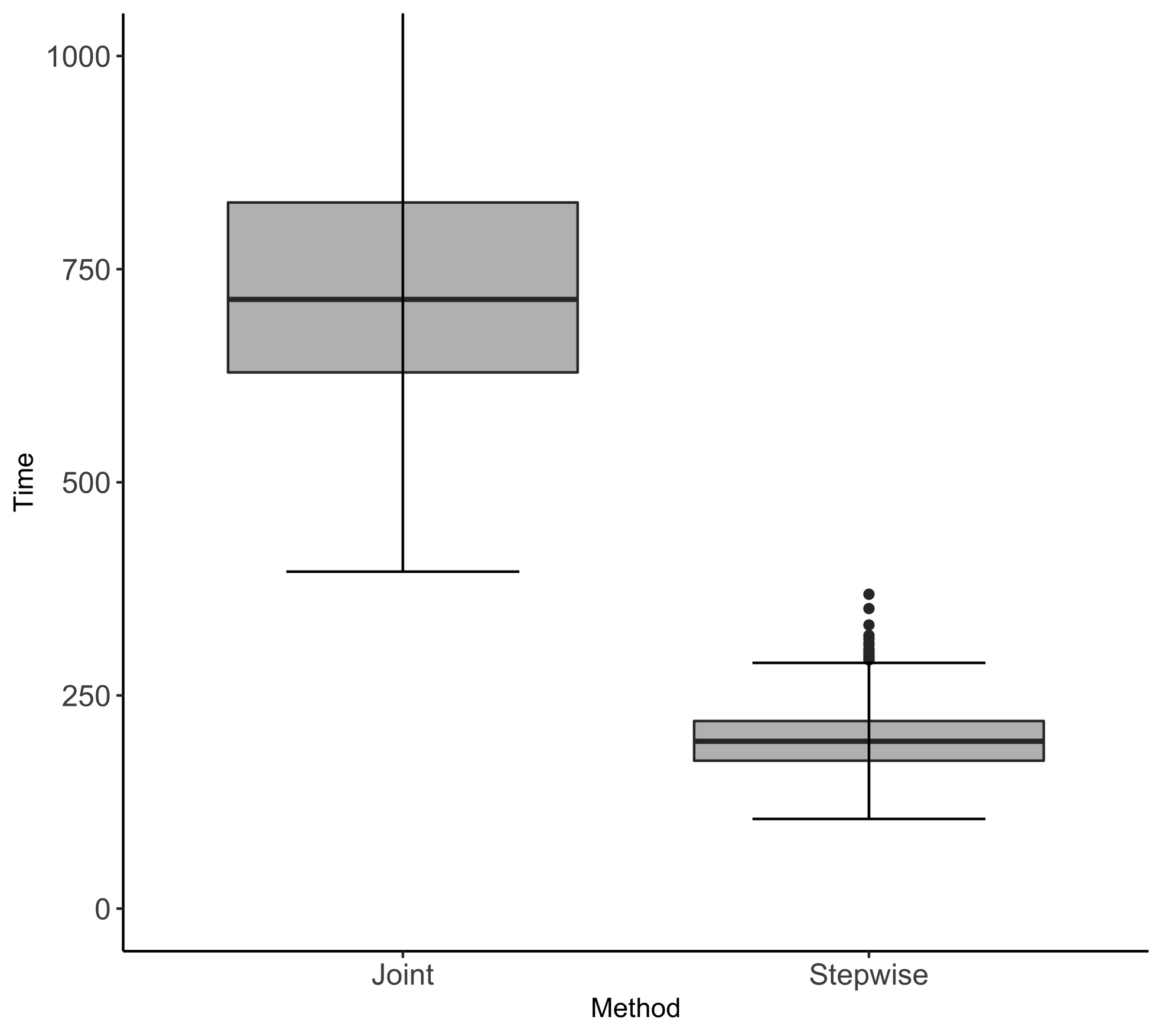
Figure 1. The box plot of the computation loads for calculating the joint GQMLE and the stepwise GQMLE in $N=1000$ for $1000$ iterations.

Table 2. The mean bias and the standard deviation (SD) of the joint GQMLE and the stepwise GQMLE for $1000$ iterations.

	Joint GQMLE		Stepwise GQMLE
Parameter	$N=500$	$N=1000$	$N=500$	$N=1000$
$\beta_{1}$	-0.002 (0.118)	-0.001 (0.086)	0.000 (0.116)	-0.001 (0.083)
$\beta_{2}$	0.000 (0.003)	0.000 (0.002)	0.000 (0.003)	0.000 (0.002)
$\beta_{3}$	-0.001 (0.164)	0.001 (0.117)	-0.003 (0.160)	-0.001 (0.115)
$\gamma$	-0.002 (0.283)	-0.010 (0.206)	-0.008 (0.283)	-0.015 (0.204)
$\lambda$	-0.001 (0.725)	0.043 (0.733)	1.110 (10.065)	0.250 (1.074)
$\sigma$	0.000 (0.215)	0.013 (0.217)	0.331 (2.994)	0.074 (0.320)
$\sigma_{\epsilon}$	0.002 (0.008)	0.001 (0.006)	-0.002 (0.009)	-0.001 (0.006)

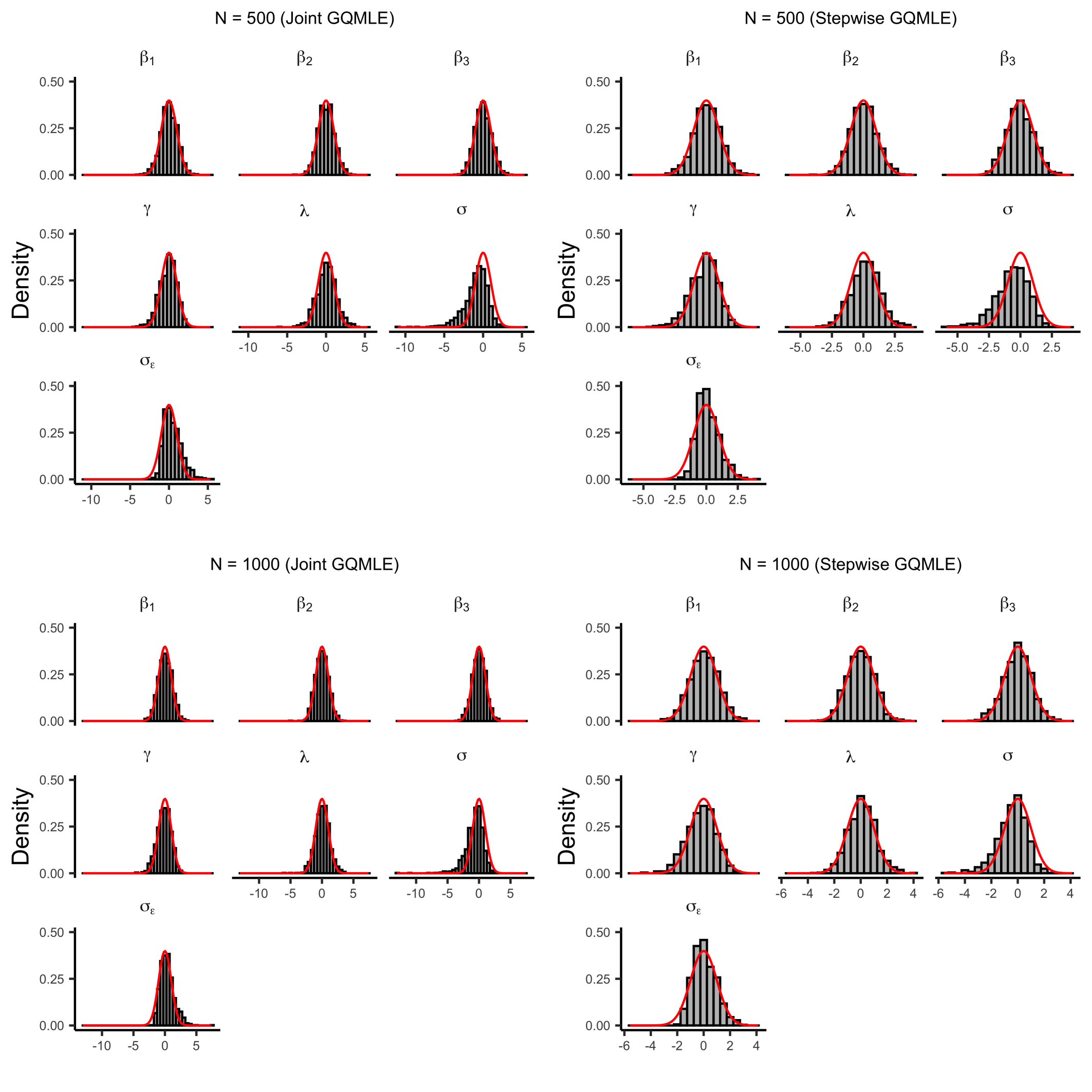
Figure 2. Histograms of the studentized joint GQMLE and the studentized stepwise GQMLE and probability density function of standard Gaussian distribution (red curve)

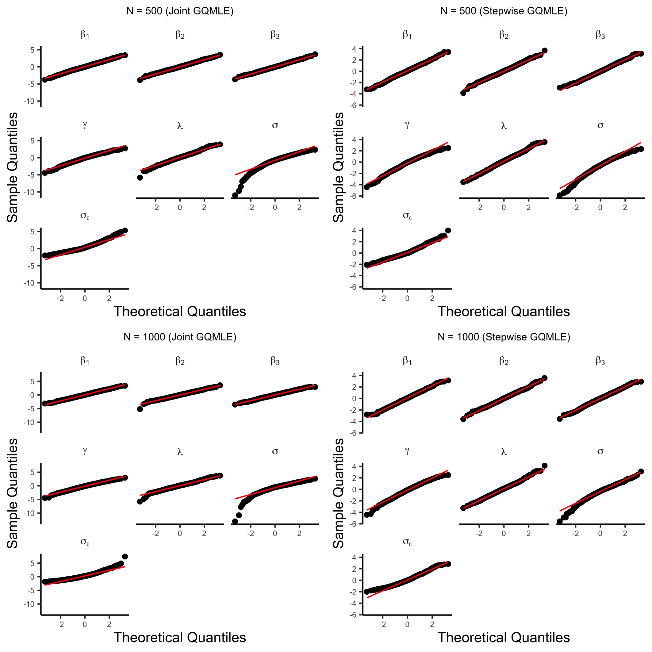
Figure 3. Normal Q-Q plots of the studentized joint GQMLE and the studentized stepwise GQMLE

6. Concluding remarks

In this paper, we considered the asymptotic behavior of the joint and stepwise GQMLE for the class of possibly non-Gaussian linear mixed-effect models. We proved that both estimators have the asymptotic normality with the same asymptotic covariance matrix and the tail-probability estimate. Moreover, we showed that the quantitative difference in the second-order terms of the joint and stepwise GQMLEs: the equation (2.14) in Theorem 2.9 and the equations (1) and (1) in Theorem 3.1. This should be informative in studying the cAIC which involves the second-order stochastic expansion of the estimator. We also note that, as we mentioned in [6, Remark 2.5], instead of the intOU we could consider the fractional Brownian motion to model the system noise for each individual.

The numerical experiments showed that the joint and stepwise GQMLEs have competitive performance with the asymptotic normality. Furthermore, the computation time for the stepwise GQMLE is much shorter than that for the joint GQMLE, hence recommended in practice.

Acknowledgements. This work was partially supported by JST CREST Grant Number JPMJCR2115 and JSPS KAKENHI Grant Numbers 22H01139, Japan.

References

- [1] R. A. Adams and J. J. F. Fournier. Sobolev spaces, volume 140 of Pure and Applied Mathematics (Amsterdam). Elsevier/Academic Press, Amsterdam, second edition, 2003.
- [2] W. J. Boscardin, J. M. Taylor, and N. Law. Longitudinal models for AIDS marker data. Statistical Methods in Medical Research, 7(1):13–27, 1998.
- [3] S. Eguchi and H. Masuda. Schwarz type model comparison for LAQ models. Bernoulli, 24(3):2278–2327, 2018.
- [4] S. Eguchi and H. Masuda. Gaussian quasi-information criteria for ergodic Lévy driven SDE. Ann. Inst. Statist. Math., 76(1):111–157, 2024.
- [5] R. A. Hughes, M. G. Kenward, J. A. C. Sterne, and K. Tilling. Estimation of the linear mixed integrated Ornstein-Uhlenbeck model. J. Stat. Comput. Simul., 87(8):1541–1558, 2017.
- [6] T. Imamura, H. Masuda, and H. Tajima. On local likelihood asymptotics for Gaussian mixed-effects model with system noise. Statist. Probab. Lett., 208:Paper No. 110074, 5, 2024.
- [7] M. Kessler, A. Schick, and W. Wefelmeyer. The information in the marginal law of a Markov chain. Bernoulli, 7(2):243–266, 2001.
- [8] T. Kubokawa. Conditional and unconditional methods for selecting variables in linear mixed models. J. Multivariate Anal., 102(3):641–660, 2011.
- [9] N. M. Laird and J. H. Ware. Random-effects models for longitudinal data. Biometrics, pages 963–974, 1982.
- [10] J. R. Magnus and H. Neudecker. The Commutation Matrix: Some Properties and Applications. The Annals of Statistics, 7(2):381 – 394, 1979.
- [11] H. Masuda. On multidimensional Ornstein-Uhlenbeck processes driven by a general Lévy process. Bernoulli, 10(1):97–120, 2004.
- [12] H. Masuda. Ergodicity and exponential -mixing bounds for multidimensional diffusions with jumps. Stochastic Process. Appl., 117(1):35–56, 2007.
- [13] H. Masuda, L. Mercuri, and Y. Uehara. Quasi-likelihood analysis for Student-Lévy regression. arXiv:2306.16790, 2023.
- [14] C. E. McCulloch and J. M. Neuhaus. Misspecifying the shape of a random effects distribution: Why getting it wrong may not matter. Statistical Science, 26:388–402, 2011.
- [15] C. E. McCulloch and J. M. Neuhaus. Prediction of random effects in linear and generalized linear models under model misspecification. Biometrics, 67(1):270–279, 2011.
- [16] S. Müller, J. L. Scealy, and A. H. Welsh. Model selection in linear mixed models. Statist. Sci., 28(2):135–167, 2013.
- [17] J. M. G. Taylor, W. G. Cumberland, and J. P. Sy. A stochastic model for analysis of longitudinal aids data. Journal of the American Statistical Association, 89(427):727–736, 1994.
- [18] F. Vaida and S. Blanchard. Conditional Akaike information for mixed-effects models. Biometrika, 92(2):351–370, 2005.
- [19] N. Yoshida. Polynomial type large deviation inequalities and quasi-likelihood analysis for stochastic differential equations. Ann. Inst. Statist. Math., 63(3):431–479, 2011.