A Cognac shot to forget bad memories:
Corrective Unlearning in GNNs

Abstract

Graph Neural Networks (GNNs) are increasingly being used for a variety of ML applications on graph data. Because graph data does not follow the independently and identically distributed (i.i.d.) assumption, adversarial manipulations or incorrect data can propagate to other data points through message passing, which deteriorates the model’s performance. To allow model developers to remove the adverse effects of manipulated entities from a trained GNN, we study the recently formulated problem of Corrective Unlearning. We find that current graph unlearning methods fail to unlearn the effect of manipulations even when the whole manipulated set is known. We introduce a new graph unlearning method, Cognac, which can unlearn the effect of the manipulation set even when only 5% of it is identified. It recovers most of the performance of a strong oracle with fully corrected training data, even beating retraining from scratch without the deletion set while being 8x more efficient. We hope our work assists GNN developers in mitigating harmful effects caused by issues in real-world data post-training. Our code is publicly available at https://github.com/varshitakolipaka/corrective-unlearning-for-gnns

1 Introduction

Graph Neural Networks (GNNs) are seeing widespread adoption across diverse domains, from recommender systems to drug discovery (Wu et al., 2022; Zhang et al., 2022). Recently, GNNs are being scaled to large training sets for graph foundation models (Mao et al., 2024). However, in these large-scale settings, it is prohibitively expensive to verify the integrity of every sample in the training data that can potentially affect desiderata like fairness (Konstantinov & Lampert, 2022), robustness (Paleka & Sanyal, 2023; Günnemann, 2022), and accuracy (Sanyal et al., 2021).

Making the training process robust to minority populations (Günnemann, 2022; Jin et al., 2020) is challenging and can adversely affect fairness and accuracy (Sanyal et al., 2022). Consequently, model developers may want post-hoc ways to remove the adverse impact of manipulated training data if they observe problematic model behavior on specific distributions of test-time inputs. Such an approach follows the recent trend of using post-training interventions to ensure models behave in intended ways (Ouyang et al., 2022). Recently, Goel et al. (2024) formulated corrective unlearning as the challenge of removing adverse effects of manipulated data with access to only a representative subset for unlearning while being agnostic to the type of manipulations. We study this problem in the context of GNNs, which face unique challenges due to the graph structure. The traditional assumption of independent and identically distributed (i.i.d.) samples does not hold for GNNs, as they use a message-passing mechanism that aggregates information from neighbors. This process makes GNNs vulnerable to adversarial perturbations, where modifying even a few nodes can propagate changes across large portions of the graph and result in widespread changes in model predictions (Bojchevski & Günnemann, 2019b; Zügner et al., 2018). Consequently, for GNNs to effectively unlearn, they must remove the influence of manipulated entities on their neighbors.

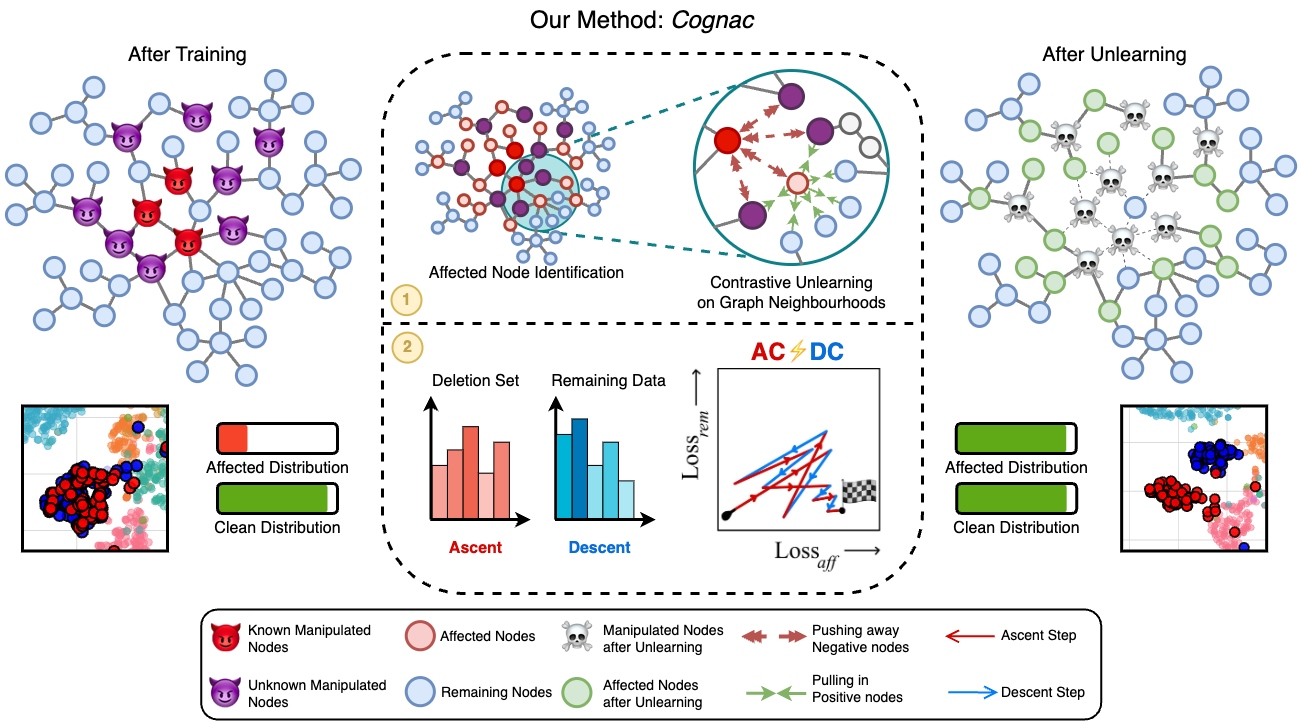
Figure 1: Illustration of our method Cognac. Initially (Left), the model is trained on manipulated data (Devils), out of which only a subset is identified for deletion (Dark-red-devils). Our method alternates between two steps. The first step (1) identifies neighbors by the deletion set, which can include both nodes from the remaining data (Light-red) and unidentified manipulated nodes (Purple), and pushes their representation away from the deletion set and toward other nodes in the neighborhood. The second step (2) performs ascent on the deletion set labels, and descent on the remaining data with separate optimizer instances. This cleanly separates the embeddings of the affected classes (Right), resulting in improved accuracy on the affected distribution, while maintaining it on the remaining distribution.

Corrective Unlearning is the problem of removing the influence of arbitrary training data manipulations on a trained model using only a representative subset of the manipulated data. In this work, we focus on the use of GNNs in node classification tasks, studying unlearning for targeted binary class confusion attacks (Lingam et al., 2024) on both edges and nodes. For edge unlearning, we evaluate the unlearning of spurious edges that change the graph topology in a way that violates the homophily assumption that most GNNs rely on. For node unlearning, we utilize a label flip attack (Lingam et al., 2024) which is used as a classical graph adversarial attack, similar to the Interclass Confusion attack (Goel et al., 2022).

First, we evaluate whether existing GNN unlearning methods are effective in removing the impact of manipulated entities. Our findings reveal that these methods consistently fail, even when provided with a complete set of manipulated entities. We then propose our method, Cognac, which unlearns by alternating between two components, as illustrated in Figure 1. The first component Contrastive unlearning on Graph Neighborhoods (CoGN), finds affected neighbors of the known deletion set, updating the GNN weights using a contrastive loss that pushes representations of the affected neighbors away from the deletion entities while staying close to other neighbors. The second component, AsCent DesCent de$\lightning$coupled (AC$\lightning$DC) applies the classic i.i.d. unlearning method of gradient ascent on the deletion set and gradient descent on the retain set. We use separate optimizers for these components as we find it essential for stable dynamics when optimizing the competing objectives.

Our proposed method shows promising results, recovering most of the performance of an oracle model with access to a clean label version of the full graph, even if only 5% of the manipulated entities are identified. This is the first corrective unlearning method for GNNs that succeeds in removing adversarial class confusion with a small fraction of the manipulated set. Finally, we perform detailed analysis with ablations, where we identify an interesting tradeoff specific to corrective unlearning on graphs. Particularly, using a larger fraction of the manipulation set for deletion while helpful for unlearning, can remove more structural information from the graph. Keeping the manipulated entities but removing the effect of their features and labels helps our method match the performance of an Oracle supplied with clean data with no manipulations. Overall, Cognac offers users of GNNs an efficient, highly effective post-training strategy to remove the adverse effects of manipulated data.

2 Related Work

Graph-based attacks, such as Sybil (Douceur, 2002) and link spam farms (Wu & Davison, 2005), have long affected the integrity of social networks and search engines by exploiting the trust inherent in node identities and edge formations. Recent works reveal that even state-of-the-art GNN architectures are vulnerable to simple attacks on the trained models which either manipulate existing edges and nodes or inject new adversarial nodes (Sun et al., 2019; Dai et al., 2018; Zügner & Günnemann, 2019; Geisler et al., 2024). Parallelly, works have characterized the influence of specific nodes and edges that can guide such attacks (Chen et al., 2023). One strategy to mitigate the influence of such attacks is robust pretraining, such as using adversarial training (Yuan et al., 2024; Zhang et al., 2023). Post-hoc interventions like unlearning act as a complementary layer of defense, helping model developers when attacks slip through and still adversely affect a trained model.

Removing the impact of manipulated entities begins with their identification (Brodley & Friedl, 1999), for which multiple strategies exist like data attribution (Ilyas et al., 2022), adversarial detection, and automated or human-in-the-loop anomaly detection (Northcutt et al., 2021). Once identified, various approaches have been proposed to edit models to remove the effects of the manipulated data, including model debiasing (Fan et al., 2024) and concept erasure (Belrose et al., 2023). While these approaches have similar goals as unlearning of post-hoc removing undesirable effects of corrupted training data, unlearning attempts to do this without precise knowledge of the nature of corruption and its effects. This is useful in adversarial settings where effects can be obfuscated, and harm multiple desiderata simultaneously (Paleka & Sanyal, 2023).

Machine unlearning gained initial interest for privacy applications to serve user data deletion requests (Nguyen et al., 2022). Exact Unlearning procedures remove or retrain parts of the ML system that saw the data to be deleted, guaranteeing perfect unlearning by design (Chen et al., 2022b; a; Bourtoule et al., 2021). However, they can incur exponential costs with sequential deletion requests (Warnecke et al., 2023). Therefore, we focus on Inexact Unlearning methods, which either provide approximate guarantees for simple models (Chien et al., 2022; Wu et al., 2023b) or like us, empirically show unlearning through evaluations for deep neural networks (Wu et al., 2023a; Cheng et al., 2023; Li et al., 2024c). Due to the non-i.i.d. nature of graphs, GNN unlearning methods need to remove the effects of deletion set entities on the remaining entities, which distinguishes the subdomain of Graph Unlearning (Said et al., 2023).

Recently, machine unlearning has received newfound attention beyond privacy applications (Pawelczyk et al., 2024; Schoepf et al., 2024; Li et al., 2024a; b). Goel et al. (2024) demonstrated the distinction between the Corrective and Privacy-oriented unlearning settings for i.i.d. classification tasks, emphasizing challenges when not all manipulated data is identified for unlearning. In this work, we focus on the intersection of corrective unlearning for graphs, evaluating existing methods, and making significant progress through our proposed method Cognac.

3 Corrective Unlearning for Graph Neural Networks

We now formulate the Corrective Unlearning problem for graph-structured, non-i.i.d. data. We consider a graph $\mathcal{G}=(\mathcal{V},\mathcal{E})$, where $\mathcal{V}$ and $\mathcal{E}$ represent the constituent set of nodes and edges respectively. For each node $\mathcal{V}_{i}\ \mathcal{\in}\ \mathcal{V}$, there is a corresponding feature vector $\mathcal{X}_{i}$ and label $\mathcal{Y}_{i}$, with $\mathcal{V}=(\mathcal{X},\mathcal{Y})$. Consistent with prior work in unlearning on graphs (Wu et al., 2023a; Li et al., 2024c), we focus on semi-supervised node classification using GNNs. GNNs use the message-passing mechanism, where each node aggregates features from its immediate neighbors. The effect of this aggregation process propagates through multiple successive layers, effectively expanding the receptive field of each node with network depth. This architecture inherently exploits the principle of homophily, a common property in many real-world graphs where nodes with similar features or labels are more likely to be connected than not.

While assuming homophily is extremely useful for learning representations from graph data, annotation mistakes or adversarial manipulations that create dissimilar neighborhoods or connect otherwise dissimilar nodes can easily harm the learned representations (Zügner & Günnemann, 2019). This motivates our study of post-hoc correction strategies like unlearning for GNNs. Following Goel et al. (2024), we adopt an adversarial formulation that subsumes correcting more benign mistakes.

Adversary’s Perspective. The adversary aims to reduce model accuracy on a target distribution by manipulating parts of the clean training data $\mathcal{G}$. This can be done in the following ways: (1) adding spurious edges $\hat{\mathcal{E}}$, resulting in $\mathcal{E}^{\prime}=\mathcal{E}\cup\hat{\mathcal{E}}$; or (2) manipulating node information, $\mathcal{V}^{\prime}=f_{m}(\mathcal{V})$, where $f_{m}$ manipulates a subset of nodes by changing their features or labels. We define $S_{m}$ as the set of manipulated entities, either the manipulated subset of nodes or the added spurious edges $\hat{\mathcal{E}}$. The final manipulated graph is denoted as $\mathcal{G}^{\prime}=(\mathcal{V}^{\prime},\mathcal{E}^{\prime})$.

Unlearner’s Perspective. After training, model developers may observe that desired properties like fairness and robustness are compromised in the trained model $\mathcal{M}$, which can be modeled as lower accuracy on some data distributions. The objective, then, is to remove the influence of the manipulated training data $S_{m}$ on the affected distribution while maintaining performance on the remaining entities. By utilizing data monitoring strategies on a subset of the training data or using incorrect data detection techniques like (Northcutt et al., 2021), it may be possible to identify a part of the manipulated entities $S_{f}\subseteq S_{m}$. For unlearning to be feasible, $S_{f}$ must be a representative subset of $S_{m}$. We only assume the type of affected entity (edges or nodes) is known to the model developer but do not assume any knowledge about the nature of manipulation. An unlearning method $U(\mathcal{M},S_{f},\mathcal{G}^{\prime})$ is then used to mitigate the adverse effects of $S_{m}$, ideally by improving the accuracy on unseen samples from the affected distribution. An effective unlearning method should remove the impact of certain training data samples without degrading performance on the rest of the data or incurring the cost of retraining from scratch. Moreover, while Retrain was previously considered a gold standard in privacy-oriented unlearning and graph unlearning, Goel et al. (2024) showed that when the whole manipulated set is not known, retraining on the remaining data can reinforce the manipulation, implying it’s not a gold standard for corrective unlearning.

Metrics. To evaluate the performance of unlearning methods in this setting, we use the metrics proposed by Goel et al. (2024):

1. $\mathrm{Acc}_{\mathrm{aff}}:$ It measures the clean-label accuracy of test set samples from the affected distribution. This metric captures the method’s ability to correct the influence of the manipulated entities on unseen data through unlearning. As the affected distribution differs for each manipulation, we specify it when describing each evaluation.

2. $\mathrm{Acc}_{\mathrm{rem}}:$ It is defined as the accuracy of the remaining entities. This metric measures whether the unlearning maintains model performance on clean entities.

The metrics $\mathrm{Acc}_{\mathrm{aff}}$ and $\mathrm{Acc}_{\mathrm{rem}}$ were termed “Corrected Accuracy” ($\mathrm{Acc}_{\mathrm{corr}}$) and “Retain Accuracy” ($\mathrm{Acc}_{\mathrm{retain}}$) respectively by Goel et al. (2024). We chose alternative names to explicitly state which data distribution accuracy is measured. In Section 5, we further specify what the “affected distribution” and “remaining entities” are for the different evaluation types we study.

Goal. An ideal corrective unlearning method should have high $\mathrm{Acc}_{\mathrm{aff}}$ even when a small fraction of manipulated set ($S_{m}$) is identified for deletion ($S_{f})$ without big drops in $\mathrm{Acc}_{\mathrm{rem}}$, all while being computationally efficient.

4 Our Method: Cognac

Our proposed unlearning method, Cognac, requires access to the underlying graph $\mathcal{G}^{\prime}$, the known set of entities to be deleted $S_{f}$, and the original model $\mathcal{M}$. We define $\mathcal{V}_{f}$ as the set of nodes whose influence is to be removed. For node unlearning, this is the same as the deletion entities $S_{f}$; for edge unlearning, this is the set of vertices connected to the edge set to be deleted. Manipulated data has two main adverse effects on the trained GNN: 1) Message passing can propagate the influence of the manipulated entities $S_{m}$ on their neighborhood, and 2) The layers learn transformations to fit potentially wrong labels in $S_{m}$. We tackle these two problems using separate components, and in Figure 10 we show that these components of our method converge.

4.1 Removing Adverse Effects on Neighboring Nodes with CoGN

The first question we address is: How can we remove the influence of manipulated entities on their neighboring nodes? This requires us first to identify the nodes affected by the manipulations and then mitigate the influence on their representations. Identifying affected nodes is challenging, as the impact of message passing from manipulated entities $S_{m}$ depends on the interference from messages of other neighboring nodes. Therefore, we use an empirical estimation to identify the affected nodes from each entity in the deletion set. On these nodes, we then perform contrastive unlearning, simultaneously pushing the representations of the affected nodes away from nodes in $\mathcal{V}_{f}$ while keeping them close to other nodes in their neighborhood. We call this component Contrastive unlearning on Graph Neighborhoods (CoGN), formalized below.

Affected Node Identification. To speed up our method, we make use of the fact that not all nodes in the $n$-hop neighborhood of the manipulated nodes may be affected enough by the attack. To find the most affected nodes, we invert the features of $v\in V_{f}$ and select neighboring nodes where final output logits are changed the most. Formally, the inversion is performed by the transformation $\vec{1}-\mathcal{X}_{v}\ \forall$ $v\in\ \mathcal{V}_{f}$, leading to a new feature matrix $\chi^{\prime}$, where $\mathcal{X}_{v}$ represents a one-hot-encoding vector. We then compute the difference in the original output logits $\mathcal{M}({\chi})$, and those obtained by on the new feature matrix, $\mathcal{M}({\chi^{\prime}})$ given by: $\Delta\mathcal{\chi}=|\mathcal{M}({\chi^{\prime}})-\mathcal{M}(\chi)|$. The top $k\%$ nodes with the most change $\Delta\mathcal{\chi}$ are selected as the affected set of entities, from which we remove the influence of the manipulation using CoGN. More details and ablations in Appendix D.2 confirm that our design choices for this, while simple and computationally cheaper, retain the same performance as using the entire $n$-hop neighborhood (Figure 12) and robustly work even if the original GNN was under-trained (Figure 11).

Contrastive Unlearning. To remove the influence of the deletion set $S_{f}$ on the affected nodes identified in the previous step, we can optimize a loss function that updates the weights such that the final layer logits of $S_{f}$ and the affected nodes are pushed away. However, this alone will lead to unrestricted separation and damage the quality of learned representations. To prevent this, we also counterbalance the loss with another term that penalizes moving away from logits of neighboring nodes not in the deletion set $S_{f}$. For each node $v\in\mathcal{S}$, let $z_{v}$ represent its internal embedding, with $p\in\mathcal{N}(v)$ and $n\in\mathcal{V}_{f}$ serving as the positive and negative samples, respectively. We use the following unsupervised contrastive loss:

$$\mathcal{L}_{c}=-\log(\sigma(z_{v}^{\top}z_{p}))-\log(\sigma(-z_{v}^{\top}z_{n}))$$ (1)

The loss is similar to the one used in GraphSAGE (Hamilton et al., 2017), but only updates affected nodes to make their representations dissimilar from the deletion set while keeping them similar to the remaining nodes in their neighborhood. We choose an unsupervised loss function to fix representations even in mislabeling, which is essential when the manipulated set is not fully known ($S_{f}\subset S_{m}$).

4.2 Unlearning old labels with AC$\lightning$DC

Next, we ask: Can we undo the effect of the task loss $\mathcal{L}_{\mathrm{task}}$ explicitly learning to fit the node representations of $S_{m}$ to potentially wrong labels? We do this by performing gradient ascent on $S_{f}$, which non-directionally maximizes the training loss concerning the old labels. Ascent alone aggressively leads to arbitrary forgetting of useful information, so we counterbalance it by alternating with steps that minimize the task loss on the remaining data. More precisely, we perform gradient ascent on $\mathcal{V}_{f}$ and gradient descent on $\mathcal{V}_{r}$, iteratively on the original GNN $\mathcal{M}$.

$$\mathcal{L}_{a}=-\mathcal{L}_{\mathrm{task}}(\mathcal{V}_{f}),\ \mathcal{L}_{d}=\mathcal{L}_{\mathrm{task}}(\mathcal{V}_{r})$$ (2)

While variants of ascent on $S_{f}$ and descent on remaining data have been studied for image classification (Kurmanji et al., 2023) and language models (Yao et al., 2023), we find the need for a specific optimization strategy to achieve corrective unlearning on graphs. The challenge arises when $S_{f}\subset S_{m}$, as the remaining data could still contain manipulated entities, which we aim to avoid reinforcing. However, in realistic scenarios, the manipulated entities $S_{m}$ typically constitute a small fraction of the training data, allowing us to mitigate their impact through ascent on the representative subset $S_{f}$.

This requires a careful balance between ascent and descent, which we can achieve by using two different optimizers and starting learning rates for these steps. This insight is similar to prior work in Generative Adversarial Networks (GANs) (Heusel et al., 2017). The starting learning rates for both ascent and descent are hyperparameters to be tuned, and usually, we find a lower learning rate for ascent leads to better results. The importance of decoupling optimizers is shown by results in Table 3. Thus, we call this component Ascent Descent de$\lightning$coupled (AC$\lightning$DC) to emphasize the distinction from existing variants of ascent on $S_{f}$ and descent on remaining data.

For our final method Cognac, we alternate steps of CoGN, which fixes representations of affected neighborhood nodes, and AC$\lightning$DC, which unlearns potentially wrong labels introduced by $S_{m}$.

4.3 Formal Description of Cognac

In this section, we outline the procedure of our proposed unlearning method, Cognac, designed to effectively remove the influence of manipulated data from GNNs. First, the algorithm identifies the nodes affected by the manipulation, as well as their corresponding positive and negative samples, and then alternates between applying CoGN and AC$\lightning$DC to unlearn their influence. The key steps include identifying the affected nodes, performing contrastive learning to re-optimize the embeddings, and minimizing classification loss on the unaffected nodes while maximizing it on the discovered manipulated set ($S_{f}$). The complete algorithm is detailed in Algorithm 1.

Algorithm 1 Cognac

1:GNN $M$, Graph $G=(V,E,X)$, Deletion set $S_{f}$, Hyperparameters $\Theta$

2:Unlearned GNN $M^{*}$

3:$S\leftarrow\textsc{IdentifyAffectedNodes}(M,X,S_{f},E,\Theta)$

4:$P\leftarrow\textsc{SamplePositives}(S,E,S_{f})$

5:$N\leftarrow\textsc{SampleNegatives}(S,S_{f})$

6:// Overall unlearning process

7:for outer_epoch $=1$ to $\Theta.$total_epochs do

8:// Contrastive unlearning phase

9:     for epoch $=1$ to $\Theta.$contrast_epochs do

10:         $Z\leftarrow M(X)$

11:         $L_{c}\leftarrow\sum_{v\in S}\left(-\log(\sigma(Z_{v}^{\top}Z_{P_{v}}))-\log(\sigma(-Z_{v}^{\top}Z_{N_{v}}))\right)$

12:         $M\leftarrow\textsc{Optimize}(M,L_{c})$

13:     end for

14:// Gradient ascent on $S_{f}$, and gradient descent on $V\setminus S_{f}$

15:     for epoch $=1$ to $\Theta.\mathrm{ascent\_descent\_epochs}$ do

16:         $L_{a}\leftarrow-\textsc{CrossEntropy}(M(X)_{S_{f}},Y_{S_{f}})$

17:         $M\leftarrow\textsc{Optimize}(M,L_{a})$

18:         $L_{d}\leftarrow\textsc{CrossEntropy}(M(X)_{V\setminus S_{f}},Y_{V\setminus S_{f}})$

19:         $M\leftarrow\textsc{Optimize}(M,L_{d})$

20:     end for

21:end for

22:return $M$

23:function IdentifyAffectedNodes($M,X,S_{f},E,\Theta$)

24:     $X^{\prime}\leftarrow\textsc{InvertFeatures}(X,S_{f},E)$

25:     $\Delta\leftarrow|M(X^{\prime})-M(X)|$

26:     return $\textsc{TopK}(\Delta,\Theta.k)$

27:end function

5 Experimental Setup

5.1 Evaluations

Given a fixed budget of samples to manipulate, ideal corrective unlearning evaluations should maximally deteriorate model performance on the affected distribution so that there is a wide gap between clean and poisoned model performance to measure unlearning method progress. We thus evaluate unlearning on attacks not constrained by stealthiness. Lingam et al. (2024) show that binary label flip manipulation attacks, where a fraction of labels are swapped between two chosen classes, are stronger than multi-class manipulations, theoretically and empirically, on GNNs. Building on this, we use two targeted attacks to evaluate corrective unlearning on graph data.

Spurious Edge Addition. To evaluate edge unlearning, we first describe a graph-specific manipulation where an attacker can add edges to the graph topology (Bojchevski & Günnemann, 2019a). Such an attack can occur in real-world settings like social networks, where attackers can create fake accounts and follow targeted accounts, strengthening their connection in the underlying graph. Similarly, attackers could manipulate knowledge graphs by adding links between unrelated concepts (Xi et al., 2023; Zhang et al., 2019; Zhao et al., 2024), or manipulate search engine results by adding fake cross-references (Gyongyi & Garcia-Molina, 2005). Prior GNN unlearning works (Wu et al., 2023a; Li et al., 2024c) have also evaluated adversarial edge attacks but in an untargeted setting, making the evaluation weak. In our formulation, the attacker selects two classes, samples random pairs of nodes uniformly, with one from each class, and adds edges between them. This targets the underlying homophily assumption in message passing, leading to representations of the two classes being entangled when training the model. Hence, this attack reduces the model’s accuracy on samples from the two classes, which form the affected distribution. Thus, the unlearning goal is to improve $\mathrm{Acc}_{\mathrm{aff}}$, which is accuracy on the test set samples of the two targeted classes. For $\mathrm{Acc}_{\mathrm{rem}}$, we measure accuracy on test set samples from the remaining classes.

Label Manipulation. Next, to evaluate node unlearning, we study a label-only manipulation that models settings where model developers source external annotations on their data. We focus on systematic mislabeling, which can occur in an adversarial context where an attacker wants the model to confuse two classes due to annotator biases or misinterpretations of potentially ambiguous guidelines. We use the Interclass Confusion (IC) Test (Goel et al., 2022), where the attacker picks two classes again, swapping the labels between nodes from the two classes. This attack also entangles the representations of the two classes, reducing the model’s accuracy on them, which forms the affected distribution. Once again, the unlearning goal is to improve $\mathrm{Acc}_{\mathrm{aff}}$, which is accuracy on the test set samples of the two targeted classes. For $\mathrm{Acc}_{\mathrm{rem}}$, we measure accuracy on test set samples from the remaining classes.

5.2 Baselines

We evaluate four popular graph unlearning methods and adapt one popular i.i.d. unlearning method for graphs. For reference, we also report results for the Original model, Retrain  which trains a new model without $S_{f}$, and an Oracle  trained on the whole training set without manipulations, indicating an upper bound on what can be achieved. The Oracle has correct labels for the unlearning entities, information that the unlearning methods cannot access.

Existing Unlearning Methods. We choose five methods as baselines where unlearning incorrect data explicitly motivates the method. (1) GNNDelete (Cheng et al., 2023) adds a deletion operator after each GNN layer and trains them using a loss function to randomize the prediction probabilities of deleted edges while preserving their local neighborhood representation, keeping the original GNN weights unchanged. (2) GIF (Wu et al., 2023a) draw from a closed-form solution for linear-GNN to measure the structural influence of deleted entities on their neighbors. Then, they provide estimated GNN parameter changes for unlearning using the inverse Hessian of the loss function. (3) MEGU (Li et al., 2024c) finds the highly influenced neighborhood (HIN) of the unlearning entities and removes their influence over the HIN while maintaining predictive performance and forgetting the deletion set using a combination of losses. (4) UtU (Tan et al., 2024) proposes zero-cost edge-unlearning by removing the edges to be deleted during inference for blocking message propagation from nodes linked to these edges. Finally, we include a popular unlearning method studied in i.i.d. classification settings. (5) SCRUB (Kurmanji et al., 2023) employs a teacher-student framework with alternate steps of distillation away from the forget set and towards the retain set. For edge unlearning, we use SCRUB by taking nodes across spuriously added edges as the forget set and the rest as the retain set.

5.3 Benchmarking Details

We now describe design choices made for benchmarking, first specifying the datasets and architectures, then how to ensure a fair comparison between methods.

Models and Datasets. We report results using the Graph Convolutional Network (GCN) (Kipf & Welling, 2017) architecture and evaluate the methods on three benchmark datasets: CoraFull (Cora) (Bojchevski & Günnemann, 2017), Coauthor CS (CS) (Shchur et al., 2019), and Amazon Photos (Amazon) (McAuley et al., 2015). In Appendix C.1, we provide additional results on the Graph Attention Network (GAT) (Veličković et al., 2018) architecture. Additional experiments (Appendix C.3) for node unlearning are also conducted on DBLP (Tang et al., 2008), Physics (Shchur et al., 2019), OGB-arXiv (Wang et al., 2020) and Amazon Computers datasets (Shchur et al., 2019).

For each dataset, we extract the largest connected subgraph for our experiments. Dataset size details, the corresponding classes, and the number of entities manipulated are provided in Table 4 under Appendix A.

Ensuring a fair comparison of unlearning methods can be tricky as there are multiple desiderata: unlearning, maintaining utility, and computational efficiency, and hyperparameter tuning of the methods can particularly affect results on GNNs. Next, we describe our efforts towards this.

Unlearning Time. To simplify comparisons to just two axes, $\mathrm{Acc}_{\mathrm{aff}}$, and $\mathrm{Acc}_{\mathrm{rem}}$, we fix a maximum cutoff of time an unlearning method can take, as motivated by Maini et al. (2024). We chose this cutoff as 25% of the original model training time. We pick the best model checkpoint during training for each method, which could be achieved earlier than this. Average run times for each method reported in Figure 7 under Appendix B.2 show that Cognac’s efficiency is comparable to or better than baselines. All experiments were run on a machine with Intel Xeon CPUs and two dedicated RTX $5000$ GPUs.

Hyperparameter Tuning. We perform extensive hyperparameter tuning for all unlearning methods using Optuna (Akiba et al., 2019) with a TPESampler (Tree-structured Parzen Estimator) Algorithm. We ensure the hyperparameter ranges searched include any values specified by the authors that proposed the methods. The optimization target is an average of $\mathrm{Acc}_{\mathrm{aff}}$ and $\mathrm{Acc}_{\mathrm{rem}}$, computed on the validation set. We report averaged results across five seeds. Method-specific hyperparameter ranges and scatter plots across hyperparameters for each method are provided in Appendix B.1.

6 Results & Discussion

We now report our results, first showing comparisons of our method to existing methods across the manipulation types and datasets, followed by ablations of our method and analysis of what can be achieved in this setting. In the Appendix, we present additional experiments: (1) Node unlearning with a GAT backbone (Appendix C.1) demonstrates Cognac’s effectiveness on another architecture. (2) Robustness testing of Cognac to large $S_{f}$ sizes (Appendix C.2) shows strong performance even with $29.4\%$ of total training nodes in $S_{f}$. (3) Node unlearning on large datasets (Appendix C.3) from Section 5.3 confirms Cognac as a top performer across diverse dataset sizes and network densities.

Table 1: Accuracy on remaining distribution for datasets and attacks. We calculate the average accuracy on the remaining classes $\mathrm{Acc}_{\mathrm{rem}}$ across the deletion set sizes tested and report the difference from Original as ideal unlearning methods should perform similarly or better. We find prior methods, especially GNNDelete and GIF, lead to large drops in $\mathrm{Acc}_{\mathrm{rem}}$, while our proposed methods Cognac and AC$\lightning$DC minimize the loss in $\mathrm{Acc}_{\mathrm{rem}}$.

Method	Amazon		CS		Cora
	Node	Edge	Node	Edge	Node	Edge
Original	[HTML]FFFFFF$94.0_{\pm 0.0}$	[HTML]FFFFFF$94.9_{\pm 0.0}$	[HTML]FFFFFF$90.4_{\pm 0.0}$	[HTML]FFFFFF$89.9_{\pm 0.0}$	[HTML]FFFFFF$56.0_{\pm 0.0}$	[HTML]FFFFFF$55.4_{\pm 0.0}$
Cognac	[HTML]FFFEFE$-0.7_{\pm 0.5}$	[HTML]FFF6F6$-3.9_{\pm 0.0}$	[HTML]FFFDFD$-0.8_{\pm 0.4}$	[HTML]FFFCFC$-1.3_{\pm 0.1}$	[HTML]FFFFFF$0.0_{\pm 0.4}$	[HTML]FFFDFD$-1.1_{\pm 1.3}$
AC$\lightning$DC	[HTML]FFFEFE$-0.5_{\pm 0.3}$	[HTML]FFF9F9$-2.7_{\pm 0.0}$	[HTML]FFFDFD$-1.1_{\pm 0.3}$	[HTML]FFFDFD$-0.9_{\pm 0.0}$	[HTML]FFFFFF$1.5_{\pm 0.0}$	[HTML]FFFCFC$-1.4_{\pm 0.0}$
GNNDelete	[HTML]FFC1C1$-24.7_{\pm 6.1}$	[HTML]FFF9F9$-2.7_{\pm 0.5}$	[HTML]FFF2F2$-5.3_{\pm 1.1}$	[HTML]FFF3F3$-5.0_{\pm 1.1}$	[HTML]FFF0F0$-6.1_{\pm 1.4}$	[HTML]FFE2E2$-11.5_{\pm 0.1}$
GIF	[HTML]FFD0D0$-18.5_{\pm 0.1}$	[HTML]FFF7F7$-3.3_{\pm 0.1}$	[HTML]FFD0D0$-18.5_{\pm 0.5}$	[HTML]FFF6F6$-3.7_{\pm 1.7}$	[HTML]FFFDFD$-1.0_{\pm 0.4}$	[HTML]FFE9E9$-8.8_{\pm 0.7}$
MEGU	[HTML]FFEAEA$-8.5_{\pm 11.5}$	[HTML]FFFDFD$-1.1_{\pm 1.2}$	[HTML]FFFBFB$-1.7_{\pm 0.2}$	[HTML]FFFCFC$-1.5_{\pm 2.5}$	[HTML]FFEFEF$-6.5_{\pm 1.0}$	[HTML]FFFDFD$-1.0_{\pm 0.8}$
UtU	[HTML]FFFFFF$0.5_{\pm 0.1}$	[HTML]FFFFFF$0.0_{\pm 0.0}$	[HTML]FFFFFF$0.0_{\pm 0.1}$	[HTML]FFFFFF$0.0_{\pm 0.0}$	[HTML]FFFFFF$0.0_{\pm 0.0}$	[HTML]FFFFFF$0.0_{\pm 0.0}$
SCRUB	[HTML]FFE8E8$-9.4_{\pm 3.7}$	[HTML]FFFDFD$-0.8_{\pm 0.0}$	[HTML]FFFFFF$0.0_{\pm 0.2}$	[HTML]FFFEFE$-0.6_{\pm 0.0}$	[HTML]FFFEFE$-0.7_{\pm 0.2}$	[HTML]FFFFFF$0.3_{\pm 0.0}$

6.1 Main Results

Figure 2 contains unlearning measurements upon varying the fraction of the manipulation set known for unlearning $({S_{f}}/{S_{m}})$. Table 1 accompanies this with utility measurements averaged across the deletion fractions for each method. We make three main observations:

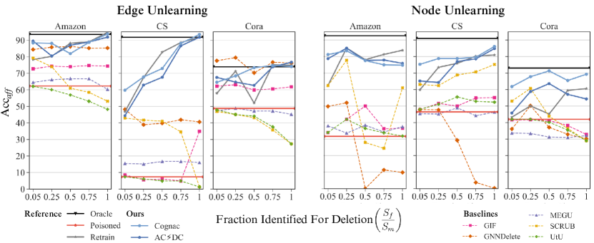
Figure 2: Corrective Unlearning Results. We report the accuracy on the affected classes $\mathrm{Acc}_{\mathrm{aff}}$ across different fractions of the manipulation set known for deletion $({S_{f}}/{S_{m}})$. Prior methods perform poorly, except for GNNDelete, which achieves reasonable unlearning performance in some settings. AC$\lightning$DC, despite not being graph-specific, performs much better. Cognac, which adds graph awareness to AC$\lightning$DC, improves results on CS and Cora, unlearning the effect of the manipulation with just 5% of the manipulation set known.

1. Existing unlearning methods perform poorly even when $|S_{f}|=|S_{m}|$. First, observing the rightmost points in Figure 2, we can see that existing methods fail to unlearn across manipulation types even when the whole manipulation set is known. The only exception is GNNDelete on the edge unlearning task, but with up to $24.7\%$ drops in $\mathrm{Acc}_{\mathrm{rem}}$ as seen in Table 1, which has also been observed before as Overforgetting in Tan et al. (2024). UtU fails to unlearn the effects of either of the attacks, as simply unlinking on the forward pass does not sufficiently counteract the influence on neighbors and weights. Both SCRUB and MEGU use a KL Divergence Loss term to keep predictions on the remaining data close to the original model, which could be detrimental when done on unidentified manipulation set entities and other affected neighbors.

2. AC$\lightning$DC shows strong results but improves with CoGN. AC$\lightning$DC, a method with no graph-specific aspects, performs quite strongly, beating all the methods we compare to without losing utility on the remaining classes. Even though MEGU and GIF were evaluated on removing adversarial edges and GNNDelete also mentioned incorrect data as one of its key applications, they failed to recover performance when presented with targeted data manipulation. Despite extensive hyperparameter searches, they are beaten by a method with no special graph components. This highlights the importance of strong evaluations for graph unlearning, a bar our evaluations cross as they at least demonstrate the failure of existing methods. These findings raise the question: are graph-specific unlearning methods even needed? Our findings imply - Yes. Cognac, which adds the graph-aware CoGN step to AC$\lightning$DC  dominates AC$\lightning$DC on CS and Cora, the more complex datasets, while performing similarly on Amazon.

3. Cognac performs strongly even at $\mathbf{5\%}$ of $\mathbf{S_{m}}$ known. We observe that Cognac performs the best across all the datasets and manipulation types, recovering most of the accuracy on the affected distribution even when $5\%$ of the manipulated set is known. We even outperform Retrain in the realistic settings when $S_{m}$ is not fully known, as we utilize negative information, i.e., push influenced neighbors away from the identified deletion set in CoGN and perform gradient ascent on old labels in AC$\lightning$DC.

Overall, these results demonstrate the efficacy of Cognac in removing different types of manipulations at a tiny fraction ($5\%$) of the manipulation set $S_{m}$ known, which shows significant progress on the challenge of corrective unlearning in the graph setting. We also visualize each method’s intermediate GNN layer embeddings after unlearning in Figure 3 where we can notice Cognac can remove the class confusion effect, fixing the model’s internal representations.

6.2 Why does $\mathrm{Acc}_{\mathrm{aff}}$ sometimes reduce as identified manipulated entities increase?

We find an interesting trend that sometimes, as more of the manipulation set $(S_{m})$ is known and used as the deletion set ($S_{f}$) (going left to right in Figure 2), $\mathrm{Acc}_{\mathrm{aff}}$ reduces. This can seem counterintuitive, as one would expect the accuracy of affected classes to improve as more samples are used for unlearning. We hypothesize that unlearning a larger fraction of the manipulation set reduces $\mathrm{Acc}_{\mathrm{aff}}$ due to two factors that adversely affect the neighborhoods of the nodes removed, which typically have other nodes of the affected classes due to homophily. First, in the case of label manipulation, when we model it as node unlearning for consistency with prior work, we lose correct information about the graph structure. Second, when modifying the graph structure, i.e., removing some edges or nodes changes the feature distribution of their neighboring nodes after the message passes, making it out of distribution for the learned GNN layers. The same rationale is why the test nodes are kept in the graph structure (without optimizing the task loss for them) during training (Kipf & Welling, 2017). We investigate this by adding an ablation where in the unlearning of the label manipulation, instead of unlearning the whole node, we keep the structure, i.e., the node and connected edges, but unlearn the features and labels.

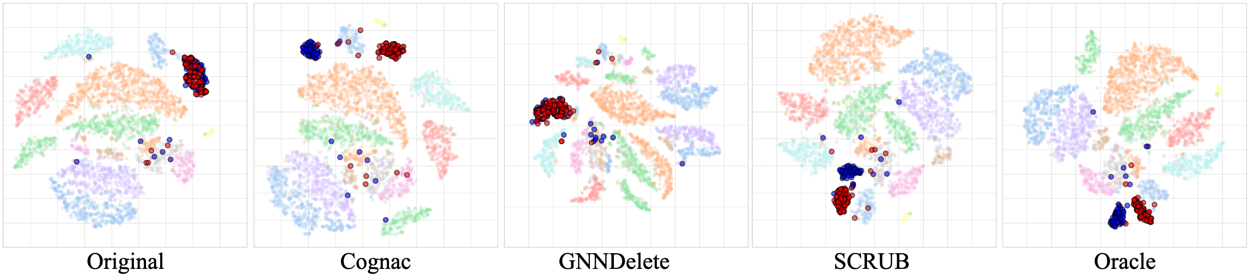
Figure 3: Pre-final layer embeddings for test nodes of the CS Dataset for the node unlearning of class confusion. Cognac can resolve the class confusion: The affected distribution embeddings (highlighted by red and blue) are fully entangled in the original trained model while after unlearning with Cognac  the embeddings are well separated and clustered. SCRUB manages to achieve the separation to a certain extent unlike GNNDelete .

Table 2: Ablating node unlearning performance on label manipulation with and without unlinking. We report the accuracy on the affected classes $\mathrm{Acc}_{\mathrm{aff}}$ for unlearning the label manipulation on Cora both when the full and a subset (25%) of the manipulated set is used for deletion. We find not removing the structural information leads to a significant improvement in $\mathrm{Acc}_{\mathrm{aff}}$, especially when more entities are deleted. This illustrates that the unlearning methods can achieve improved performance when precise information about the manipulated data is available.

Method	$\mathbf{0.25}$		$\mathbf{1.00}$
	Linked	Unlinked	Linked	Unlinked
Oracle	$73.0_{\pm 0.0}$	$73.0_{\pm 0.0}$	$73.0_{\pm 0.0}$	$73.0_{\pm 0.0}$
Original	$42.0_{\pm 0.0}$	$42.0_{\pm 0.0}$	$42.0_{\pm 0.0}$	$42.0_{\pm 0.0}$
Cognac	$\mathbf{64.8_{\pm 0.9}}$	$\mathbf{67.8_{\pm 3.2}}$	$\mathbf{77.2_{\pm 1.0}}$	$\mathbf{69.3_{\pm 1.3}}$
GNNDelete	$35.2_{\pm 2.5}$	$50.2_{\pm 1.9}$	$21.9_{\pm 4.5}$	$30.2_{\pm 5.3}$
MEGU	$40.8_{\pm 1.6}$	$33.4_{\pm 0.4}$	$41.2_{\pm 1.5}$	$32.1_{\pm 1.3}$
SCRUB	$45.7_{\pm 0.0}$	$60.7_{\pm 0.0}$	$41.1_{\pm 0.0}$	$29.0_{\pm 0.0}$
AC$\lightning$DC	$61.7_{\pm 0.0}$	$58.8_{\pm 0.0}$	$63.7_{\pm 0.0}$	$54.3_{\pm 0.0}$

As observed in Table 2, retaining the node structure leads to large improvements in $\mathrm{Acc}_{\mathrm{aff}}$ when the deletion set is larger (the full set of manipulated entities), while not benefiting much when the deletion set is smaller. In the full manipulation set deletion setting, Cognac even slightly outperforms Oracle. This highlights how—unlike conventional node unlearning in graphs—removing the nodes is not always the best way to unlearn manipulations. They can simply be moved from the train set to the test set to still partake in message passing, so the task loss is not optimized over wrong labels.

6.3 Importance of Decoupled Optimizers for Ascent and Descent

While methods incorporating gradient ascent and gradient descent have been studied in prior unlearning work like SCRUB, we find that combining these objectives into one optimizer performs sub-optimally in our experiments. Furthermore, we notice this can be fixed with a simple trick: using different learning rates for the ascent and descent steps. The final version of Cognac uses two separate optimizers: two learning rates and different instances of Adam (Kingma & Ba, 2017) instead of coupling the optimization of both steps.

To validate the necessity of separate optimizers and alternating ascent-descent we perform two ablations: (1) using a single optimizer with dual learning rates and (2) using a combined loss function instead of alternating between ascent and descent steps.

In the first ablation, since PyTorch does not provide a straightforward way to implement different LRs for the same set of parameters, we multiply the LR during ascent with a tunable constant. This is functionally equivalent to having 2 LRs as we use a linear decay schedule, which despite its simplicity was recently shown to outperform more complicated schedulers (Defazio et al., 2023).

Adding another hyperparameter for the ascent learning rate is necessary as the ascent is not always needed when the original training data labels are correct. For example, we do find that the ascent learning rate is set to nearly zero during automatic hyperparameter selection for our edge unlearning evaluation, where labels are not manipulated. In Table 3, we report results on $25\%$ and $100\%$ of the manipulated nodes identified for Cora. We find AC$\lightning$DC leads to almost $20\%$ better $\mathrm{Acc}_{\mathrm{aff}}$ than using a single optimizer with alternating ascent descent, and $5-10\%$ better $\mathrm{Acc}_{\mathrm{aff}}$ than using a combined loss function. This justifies our contribution of decoupling optimizers in AC$\lightning$DC.

Table 3: Ablations of AC$\lightning$DC at $({S_{f}}/{S_{m}})$ = 0.25 and 1.00 on Cora node unlearning. We ablate the AC$\lightning$DC  part of our method, even when the losses are combined in a single loss term.

Method	$\mathbf{0.25}$		$\mathbf{1.00}$
	$\mathrm{Acc}_{\mathrm{aff}}$	$\mathrm{Acc}_{\mathrm{rem}}$	$\mathrm{Acc}_{\mathrm{aff}}$	$\mathrm{Acc}_{\mathrm{rem}}$
Single Optimizer 1 LR Alternating Ascent Descent	$38.3$	$56.0$	$29.0$	$56.2$
Single Optimizer 2 LRs Combined Loss	$47.5$	$56.7$	$49.6$	$55.1$
AC$\lightning$DC	$58.8$	$57.4$	$54.3$	$56.1$

7 Limitations and Conclusion

In this work, we study the problem of corrective unlearning for GNNs, where model developers try to remove the adverse effects of manipulated training data from a trained GNN, with realistically only a fraction of it identified for deletion. Like previous work in the domain, our work relies on the homophily assumption, not catering to heterophilic graphs (Wang et al., 2024). Moreover, our evaluations may not fully reflect real-world scenarios, which often involve complex, simultaneous manipulations and attackers operating under constraints, such as avoiding detection. While our methods demonstrate successful unlearning within the scope of our experiments, they do not guarantee effectiveness against arbitrary real-world scenarios, particularly when facing adaptive attacks. This highlights the need for the development of stronger, more realistic attack models and evaluation frameworks in future works.

Nevertheless, our evaluations are sufficient to show that existing unlearning methods perform poorly at removing adverse effects of manipulations from GNNs, even in the unrealistic setting of the full manipulation set being known. We propose a new method Cognac  that achieves two crucial effects necessary for corrective unlearning. First, Cognac identifies and fixes representations of neighborhood nodes affected by the deletion set using contrastive loss for fine-tuning. Second, Cognac moves away from potentially wrong deletion set labels using gradient ascent, stabilized by continuing optimization of the task loss on the remaining data with a decoupled optimizer. While our method does not provide any theoretical guarantees, to the best of our knowledge, Cognac is the first method to unlearn class confusion manipulations with access to as little as $5\%$ of the manipulated data, recovering most of the accuracy on the affected distribution. With additional information, it nearly matches a strong oracle with full correct training data. We hope this sparks interesting future work on developing stronger evaluations and theoretical understanding for graph corrective unlearning in the GNN Robustness and Machine Unlearning community.

Appendix A Dataset Details

In Table 4, we discuss the number of nodes, edges, and labels, as well as manipulation statistics for all datasets used for experiments.

Table 4: Dataset and manipulation statistics. The number of nodes and edges reported here is for the whole dataset. From this, we use a 60/20/20 split for train/validation/test. The last two columns show the percentage of training data manipulated in the node unlearning and edge unlearning evaluation, respectively. The percentage of nodes and edges added are relative to the existing number of training nodes and the number of edges in the graph, respectively.

Dataset	# Classes	# Nodes	# Edges	Nodes Manipulated $\mathbf{(\%)}$	Edges Added $\mathbf{(\%)}$
Cora	$70$	$18,800$	$125,370$	$1.50$	$0.60$
CS	$15$	$18,333$	$163,788$	$2.00$	$2.00$
Amazon	$8$	$7,487$	$238,086$	$12.00$	$4.20$
DBLP	$4$	$17,716$	$105,734$	$10.0$	-
Physics	$5$	$34,493$	$495,924$	$9$	-
Computers	$10$	$13,381$	$245,778$	$3.3$	-
OGB-arXiv	$40$	$169,343$	$1,166,243$	$2.5$	-

Appendix B Method Details

B.1 Hyperparameter Tuning

We perform hyperparameter tuning for each combination for attack, dataset, unlearning method, and the identified fraction of deletion set ($S_{f}$). The optimization target is an average of $\mathrm{Acc}_{\mathrm{aff}}$ and $\mathrm{Acc}_{\mathrm{rem}}$, computed on the validation set. For each setting, we run 100 trials with hyperparameters selected using the TPESampler (Tree-structured Parzen Estimator) algorithm. In Figures 4, 5 and 6, we report $\mathrm{Acc}_{\mathrm{aff}}$ and $\mathrm{Acc}_{\mathrm{rem}}$ scores for each hyperparameter tuning trial. Across hyperparameter runs, existing graph-based unlearning methods, barring MEGU, vary drastically across different sets of hyperparameters. On the other hand, our proposed method Cognac and its ablations show consistently high scores across hyperparameters, showcasing Cognac’s robustness to hyperparameter tuning.

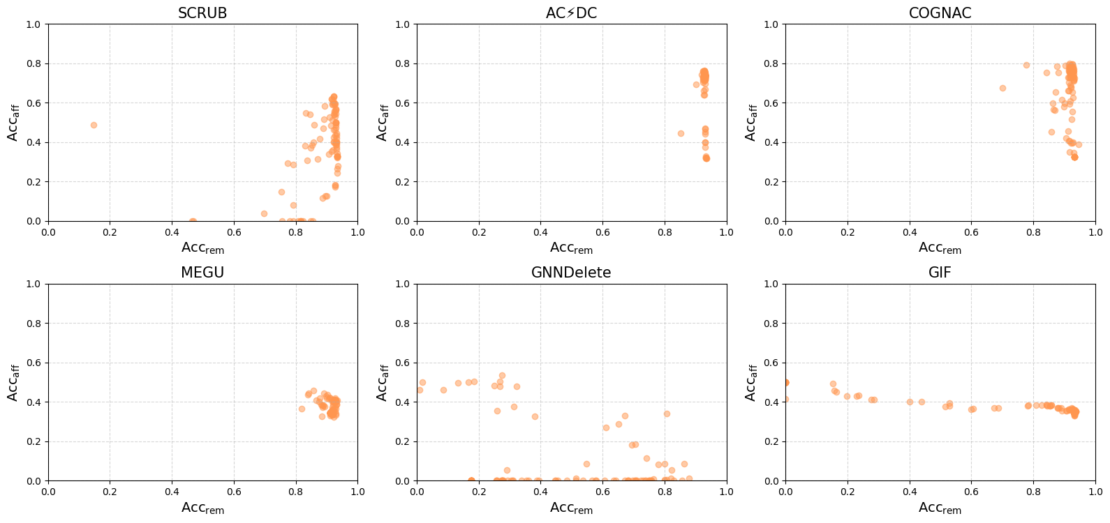
Figure 4: Hyperparameter runs for $S_{f}=1.0$ on Amazon. Scores of various hyperparameter trial runs. The best hyperparameters are selected according to the run achieving the best value for the average of $\mathrm{Acc}_{\mathrm{rem}}$ and $\mathrm{Acc}_{\mathrm{aff}}$.

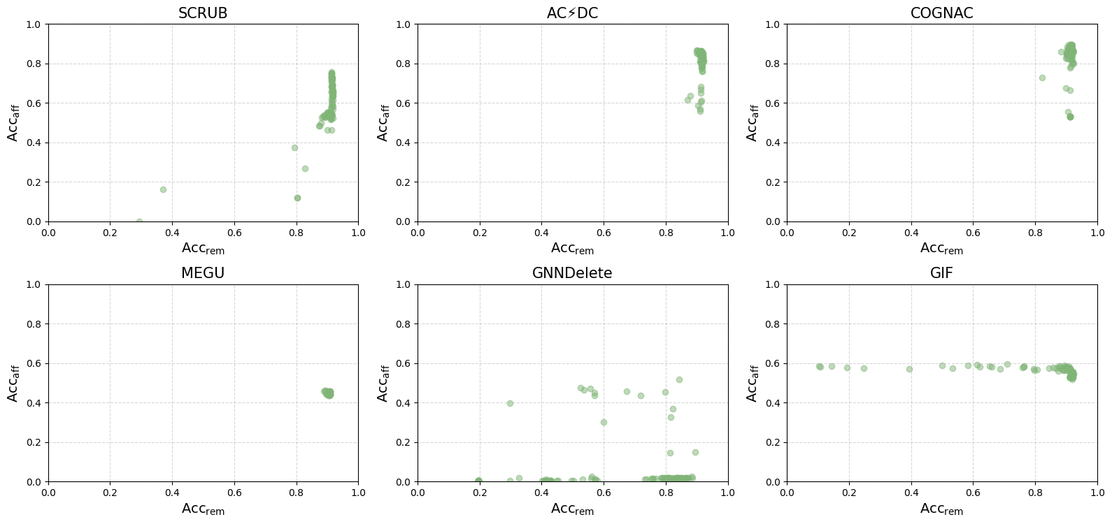
Figure 5: Hyperparameter runs for $S_{f}=1.0$ on CS. Scores of various hyperparameter trial runs. The best hyperparameters are selected according to the run achieving the best value for the average of $\mathrm{Acc}_{\mathrm{rem}}$ and $\mathrm{Acc}_{\mathrm{aff}}$.

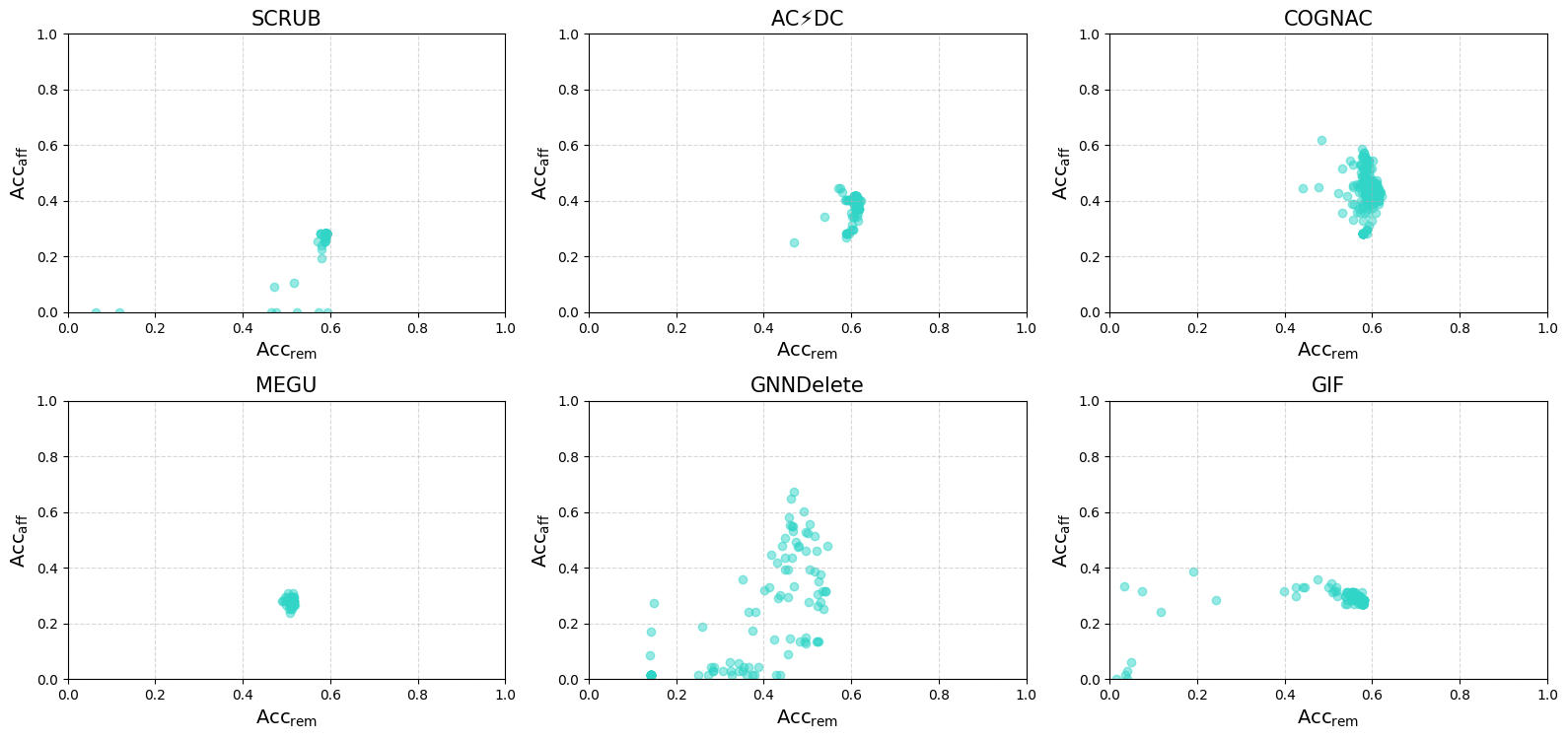
Figure 6: Hyperparameter runs for $S_{f}=1.0$ on Cora. Scores of various hyperparameter trial runs. The best hyperparameters are selected according to the run achieving the best value for the average of $\mathrm{Acc}_{\mathrm{rem}}$ and $\mathrm{Acc}_{\mathrm{aff}}$.

B.2 Unlearning Times

To ensure the practicality of inexact unlearning methods, they must achieve greater efficiency than retraining from scratch. As illustrated in Figure 7, Cognac demonstrates competitive efficiency compared to alternative methods, offering substantial speedups over retraining from scratch.

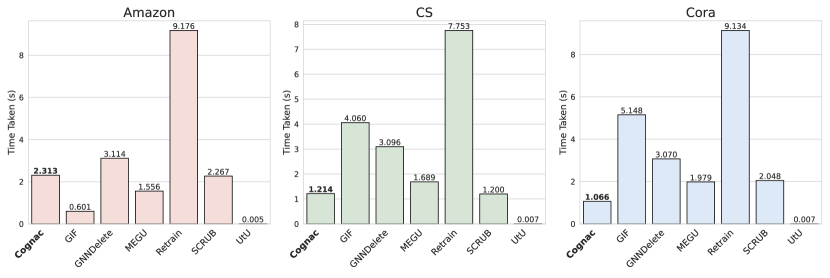
Figure 7: Time taken to unlearn. We report the time taken by each unlearning method for all datasets, in the setting where all manipulated samples are known for deletion. Cognac provides significant speedups over Retrain and has performance similar to other unlearning methods.

Appendix C Results Showing The Breadth of Applicability of Cognac 

C.1 Results on GAT

To provide a comprehensive comparison between Cognac and other methods, we provide results on commonly used GNN backbone architectures - GCN and GAT.

Graph Convolutional Network (GCN) is a method for semi-supervised classification of graph-structured data. It employs an efficient layer-wise propagation rule derived from a first-order approximation of spectral convolutions on graphs.

Graph Attention Network (GAT) employs computationally efficient masked self-attention layers that assign varying importance to neighborhood nodes without needing the complete graph structure upfront, thereby overcoming many theoretical limitations of earlier spectral-based methods.

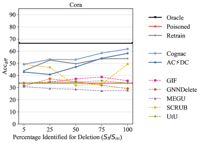
Figure 8: Node Unlearning results for Cora with GAT backbone. Comparison of $\mathrm{Acc}_{\mathrm{aff}}$ for the unlearning methods on GAT trained on Cora for different values of $({S_{f}}/{S_{m}})$. We see that Cognac outperforms all baselines.

Figure 8 shows that Cognac also performs competitively with a GAT backbone. When 5% of $S_{m}$ is known, SCRUB performs similarly to Cognac, within the standard deviation. For higher fractions, we achieve greater $\mathrm{Acc}_{\mathrm{aff}}$ than the benchmark graph unlearning methods with large margins, often beating the performance of retraining the GNN from scratch. These results indicate that benchmark graph unlearning methods used for comparison cannot recover from the impact of the label flip poison. In contrast, our method is much closer to Oracle’s performance.

C.2 Performance on large $S_{f}$

To stress-test Cognac’s performance - as methods could potentially degrade as the size of $S_{f}$ grows - we conduct an experiment where we choose a significant fraction of the training nodes of the Amazon, DBLP, and Physics datasets, to be attacked (by the binary label flip attack) and marked for deletion. The method performs competitively even at this large deletion size. Table 5 demonstrates these results.

Table 5: Evaluation on larger sizes of $S_{f}$. Cognac performs well across datasets (Amazon, DBLP, Physics), even when a significant fraction of the total training nodes are present in $S_{f}$.

Method	Amazon $(25\%)$		DBLP $(29.4\%)$		Physics $(14.8\%)$
	$\mathrm{Acc}_{\mathrm{rem}}$	$\mathrm{Acc}_{\mathrm{aff}}$	$\mathrm{Acc}_{\mathrm{rem}}$	$\mathrm{Acc}_{\mathrm{aff}}$	$\mathrm{Acc}_{\mathrm{rem}}$	$\mathrm{Acc}_{\mathrm{aff}}$
Oracle	$92.9$	$95.6$	$72.9$	$86.0$	$95.2$	$95.1$
Original	$92.5$	$49.0$	$74.9$	$57.9$	$58.9$	$95.4$
Cognac	$\mathbf{92.4}$	$\mathbf{83.7}$	$\mathbf{82.3}$	$81.7$	$\mathbf{90.7}$	$\mathbf{95.0}$
GNNDelete	$27.7$	$49.7$	$45.0$	$49.6$	$1.4$	$37.3$
SCRUB	$92.3$	$72.6$	$77.5$	$\mathbf{82.1}$	$77.9$	$94.9$

C.3 Performance on Additional Datasets

We have additionally tested our method on DBLP (Tang et al., 2008), Physics (Shchur et al., 2019), OGB-arXiv (Wang et al., 2020) and Amazon Computers datasets (Shchur et al., 2019) on the binary label flip attack (details in Table 4). As shown in Table 6 and Figure 9, Cognac is still a top performer on the new datasets, outperforming all baselines. We note that the utility is maintained by Cognac across datasets and deletion sizes.

Table 6: Results on the OGB-arXiv dataset for $S_{f}/S_{m}\mathbf{=0.25,1.00}$. We observe that the Cognac method outperforms all baseline approaches, including Retrain, in both correcting the $\mathrm{Acc}_{\mathrm{aff}}$ metric and maintaining the $\mathrm{Acc}_{\mathrm{rem}}$ metric.

Method	$\mathbf{0.25}$		$\mathbf{1.00}$
	$\mathbf{\mathrm{Acc}_{\mathrm{aff}}}$	$\mathbf{\mathrm{Acc}_{\mathrm{rem}}}$	$\mathbf{\mathrm{Acc}_{\mathrm{aff}}}$	$\mathbf{\mathrm{Acc}_{\mathrm{rem}}}$
Oracle	$66.8_{\pm 0.0}$	$49.2_{\pm 0.0}$	$66.8_{\pm 0.0}$	$49.2_{\pm 0.0}$
Original	$40.5_{\pm 0.0}$	$48.6_{\pm 0.0}$	$40.5_{\pm 0.0}$	$48.6_{\pm 0.0}$
Retrain	$54.9_{\pm 5.0}$	$46.3_{\pm 1.0}$	$59.1_{\pm 3.9}$	$44.4_{\pm 2.0}$
Cognac	$\mathbf{58.0_{\pm 0.5}}$	$\mathbf{49.6_{\pm 0.1}}$	$\mathbf{59.2_{\pm 0.7}}$	$\mathbf{49.7_{\pm 0.1}}$
SCRUB	$54.5_{\pm 1.1}$	$49.2_{\pm 0.1}$	$49.2_{\pm 0.2}$	$48.9_{\pm 0.1}$
UtU	$38.4_{\pm 0.0}$	$48.7_{\pm 0.0}$	$30.4_{\pm 0.0}$	$48.9_{\pm 0.0}$
GNNDelete	$44.3_{\pm 4.8}$	$6.0_{\pm 4.2}$	$27.4_{\pm 4.1}$	$32.0_{\pm 2.6}$

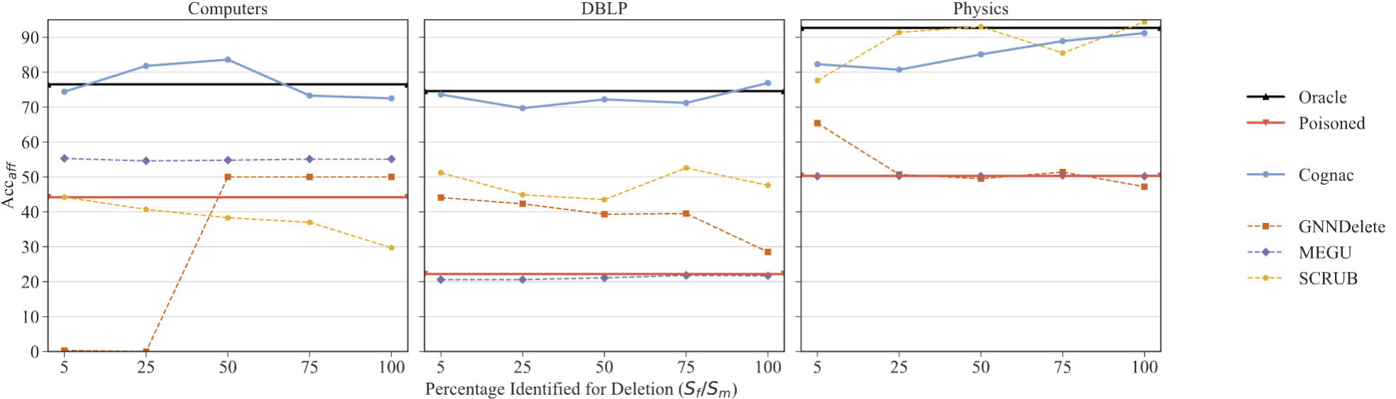
Figure 9: Evaluation on additional datasets (Computers, DBLP, Physics). Cognac still outperforms the baselines in most settings and matches Oracle’s performance on the new datasets.

Appendix D Convergence and Ablations of Cognac 

D.1 Convergence

We now discuss the convergence properties of Cognac. Plots in Figure 10 describe the losses of each of the components of our method (contrastive, ascent, descent) after the last epoch of every step, the meaning of which should be clear from Algorithm 1: Line 4 (which we denote as num_steps). The loss plots are constructed over the best hyperparameters, and we would likely not see such convergence trends with sub-optimal hyperparameters, which may provide insights to improve performance when it’s used in other settings as well.

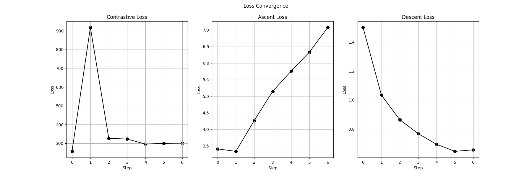
Figure 10: Convergence of the losses across unlearning steps. The ascent loss on $S_{m}$ continually increases as expected, the descent loss on $S\setminus S_{m}$ converges, and the contrastive loss exhibits a low plateau after an initial overshoot, implying it may have learned discriminative features.

D.2 Analysis of method used to find affected neighbors

Our strategy to find affected neighbors is likely not perfect for finding the most affected nodes and more sophisticated influence functions such as the one presented in Chen et al. (2023) could be used to potentially improve performance. Still, we note that it achieves a $~{}5\%$ higher $\mathrm{Acc}_{\mathrm{aff}}$ than while choosing random $k$% nodes in the $n$-hop neighborhood (where $n$ is the number of layers of message passing) while being cheap to compute: we only require a single forward pass over the model with the inverted features. Interestingly, Figure 11 also shows that even if the GNN is not well-trained, if we choose the top $k\%$ affected nodes, the unlearning performance does not change much, while still being noticeably better than when we use a random $k\%$ of the neighbors.

Figure 12 (left) shows that there are no noticeable changes in taking a smaller or larger $k\%$. However, removing this step entirely ($k=0\%$) results in worse performance, suggesting performing contrastive unlearning on even a small $k\%$ is significant. Additionally, by keeping this percentage small, we ensure computational efficiency without diminishing performance (Figure 12 (right)), which is essential for unlearning methods.

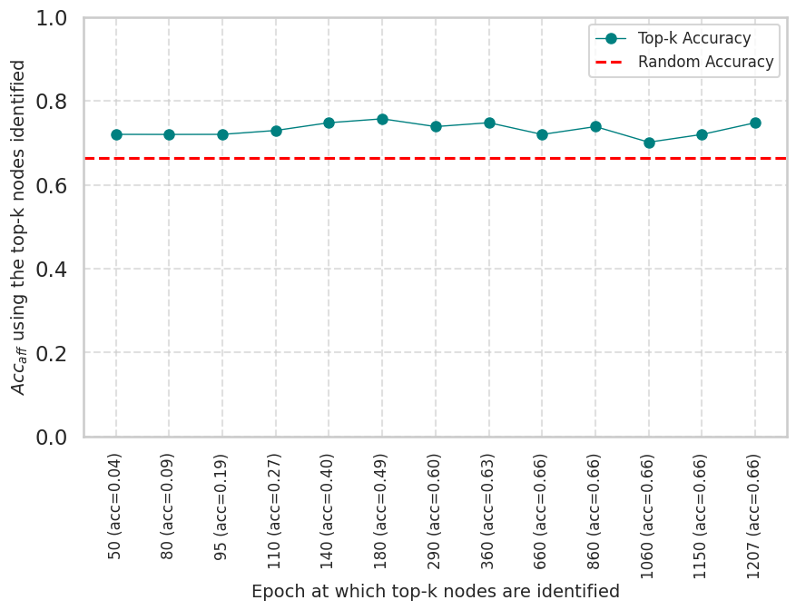
Figure 11: Effect of how well-trained the GNN is on top-$k\%$ affected neighbour identification. Here $k=4$. The x-axis represents the epoch at which we used GNN representations to identify the most affected neighbors for Cognac. The y-axis reports the unlearning performance after contrastive unlearning on these identified nodes using the final model. The red line contains performance after picking a random subset from the $n$-hop neighborhood. Affected neighborhood identification using top-$k\%$ logit change is more effective even with an extremely undertrained GNN.

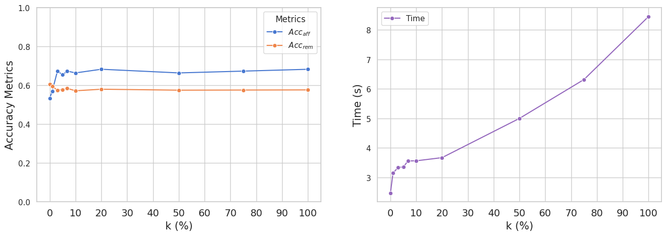
Figure 12: Effect of $k$ on unlearning ($\mathrm{Acc}_{\mathrm{aff}}$), utility ($\mathrm{Acc}_{\mathrm{rem}}$) and efficiency when identifying top-$k\%$ affected nodes for contrastive unlearning. (Left) Cognac effectiveness sharply improves beyond $k=0\%$, suggesting that performing contrastive unlearning on even a small percentage of nodes ($k$) significantly enhances the algorithm’s effectiveness. However, using higher values of $k$ yields similar performance with the added downside of increasing computational time (Right).

References

- Akiba et al. (2019) Takuya Akiba, Shotaro Sano, Toshihiko Yanase, Takeru Ohta, and Masanori Koyama. Optuna: A next-generation hyperparameter optimization framework. In Proceedings of the 25th ACM SIGKDD international conference on knowledge discovery & data mining, pp. 2623–2631, 2019.
- Belrose et al. (2023) Nora Belrose, David Schneider-Joseph, Shauli Ravfogel, Ryan Cotterell, Edward Raff, and Stella Biderman. LEACE: Perfect linear concept erasure in closed form. In Thirty-seventh Conference on Neural Information Processing Systems, 2023. URL https://openreview.net/forum?id=awIpKpwTwF.
- Bojchevski & Günnemann (2017) Aleksandar Bojchevski and Stephan Günnemann. Deep gaussian embedding of graphs: Unsupervised inductive learning via ranking. arXiv preprint arXiv:1707.03815, 2017.
- Bojchevski & Günnemann (2019a) Aleksandar Bojchevski and Stephan Günnemann. Adversarial attacks on node embeddings via graph poisoning. In International Conference on Machine Learning, pp. 695–704. PMLR, 2019a.
- Bojchevski & Günnemann (2019b) Aleksandar Bojchevski and Stephan Günnemann. Certifiable robustness to graph perturbations. Advances in Neural Information Processing Systems, 32, 2019b.
- Bourtoule et al. (2021) Lucas Bourtoule, Varun Chandrasekaran, Christopher A. Choquette-Choo, Hengrui Jia, Adelin Travers, Baiwu Zhang, David Lie, and Nicolas Papernot. Machine unlearning. In IEEE S&P, 2021.
- Brodley & Friedl (1999) Carla E Brodley and Mark A Friedl. Identifying mislabeled training data. Journal of artificial intelligence research, 11:131–167, 1999.
- Chen et al. (2022a) Chong Chen, Fei Sun, Min Zhang, and Bolin Ding. Recommendation unlearning. In Proceedings of the ACM Web Conference 2022, pp. 2768–2777, 2022a.
- Chen et al. (2022b) Min Chen, Zhikun Zhang, Tianhao Wang, Michael Backes, Mathias Humbert, and Yang Zhang. Graph unlearning. In Proceedings of the 2022 ACM SIGSAC conference on computer and communications security, pp. 499–513, 2022b.
- Chen et al. (2023) Zizhang Chen, Peizhao Li, Hongfu Liu, and Pengyu Hong. Characterizing the influence of graph elements. In The Eleventh International Conference on Learning Representations, 2023. URL https://openreview.net/forum?id=51GXyzOKOp.
- Cheng et al. (2023) Jiali Cheng, George Dasoulas, Huan He, Chirag Agarwal, and Marinka Zitnik. GNNDelete: A general unlearning strategy for graph neural networks. In International Conference on Learning Representations, 2023. URL https://openreview.net/forum?id=X9yCkmT5Qrl.
- Chien et al. (2022) Eli Chien, Chao Pan, and Olgica Milenkovic. Efficient model updates for approximate unlearning of graph-structured data. In The Eleventh International Conference on Learning Representations, 2022.
- Dai et al. (2018) Hanjun Dai, Hui Li, Tian Tian, Xin Huang, Lin Wang, Jun Zhu, and Le Song. Adversarial attack on graph structured data. In Jennifer Dy and Andreas Krause (eds.), Proceedings of the 35th International Conference on Machine Learning, volume 80 of Proceedings of Machine Learning Research, pp. 1115–1124. PMLR, 10–15 Jul 2018.
- Defazio et al. (2023) Aaron Defazio, Ashok Cutkosky, Harsh Mehta, and Konstantin Mishchenko. When, why and how much? adaptive learning rate scheduling by refinement, 2023. URL https://arxiv.org/abs/2310.07831.
- Douceur (2002) John R Douceur. The sybil attack. In International workshop on peer-to-peer systems, pp. 251–260. Springer, 2002.
- Fan et al. (2024) Shaohua Fan, Xiao Wang, Yanhu Mo, Chuan Shi, and Jian Tang. Debiasing graph neural networks via learning disentangled causal substructure. In Proceedings of the 36th International Conference on Neural Information Processing Systems, NIPS ’22, Red Hook, NY, USA, 2024. Curran Associates Inc. ISBN 9781713871088.
- Geisler et al. (2024) Simon Geisler, Tobias Schmidt, Hakan Şirin, Daniel Zügner, Aleksandar Bojchevski, and Stephan Günnemann. Robustness of graph neural networks at scale. In Proceedings of the 35th International Conference on Neural Information Processing Systems, NIPS ’21, Red Hook, NY, USA, 2024. Curran Associates Inc. ISBN 9781713845393.
- Goel et al. (2022) Shashwat Goel, Ameya Prabhu, Amartya Sanyal, Ser-Nam Lim, Philip Torr, and Ponnurangam Kumaraguru. Towards adversarial evaluations for inexact machine unlearning. arXiv preprint arXiv:2201.06640, 2022.
- Goel et al. (2024) Shashwat Goel, Ameya Prabhu, Philip Torr, Ponnurangam Kumaraguru, and Amartya Sanyal. Corrective machine unlearning. Data-centric Machine Learning Research (DMLR) Workshop, ICLR, 2024.
- Günnemann (2022) Stephan Günnemann. Graph neural networks: Adversarial robustness. Graph neural networks: foundations, frontiers, and applications, pp. 149–176, 2022.
- Gyongyi & Garcia-Molina (2005) Zoltan Gyongyi and Hector Garcia-Molina. Link spam alliances. Technical report, Stanford, 2005.
- Hamilton et al. (2017) Will Hamilton, Zhitao Ying, and Jure Leskovec. Inductive representation learning on large graphs. Advances in neural information processing systems, 30, 2017.
- Heusel et al. (2017) Martin Heusel, Hubert Ramsauer, Thomas Unterthiner, Bernhard Nessler, and Sepp Hochreiter. Gans trained by a two time-scale update rule converge to a local nash equilibrium. Advances in neural information processing systems, 30, 2017.
- Ilyas et al. (2022) Andrew Ilyas, Sung Min Park, Logan Engstrom, Guillaume Leclerc, and Aleksander Madry. Datamodels: Predicting predictions from training data. arXiv preprint arXiv:2202.00622, 2022.
- Jin et al. (2020) Wei Jin, Yao Ma, Xiaorui Liu, Xianfeng Tang, Suhang Wang, and Jiliang Tang. Graph structure learning for robust graph neural networks. In Proceedings of the 26th ACM SIGKDD international conference on knowledge discovery & data mining, pp. 66–74, 2020.
- Kingma & Ba (2017) Diederik P. Kingma and Jimmy Ba. Adam: A method for stochastic optimization, 2017. URL https://arxiv.org/abs/1412.6980.
- Kipf & Welling (2017) Thomas N. Kipf and Max Welling. Semi-supervised classification with graph convolutional networks, 2017.
- Konstantinov & Lampert (2022) Nikola H Konstantinov and Christoph Lampert. Fairness-aware pac learning from corrupted data. JMLR, 2022.
- Kurmanji et al. (2023) Meghdad Kurmanji, Peter Triantafillou, and Eleni Triantafillou. Towards unbounded machine unlearning. NeurIPS, 2023.
- Li et al. (2024a) Nathaniel Li, Alexander Pan, Anjali Gopal, Summer Yue, Daniel Berrios, Alice Gatti, Justin D Li, Ann-Kathrin Dombrowski, Shashwat Goel, Long Phan, et al. The wmdp benchmark: Measuring and reducing malicious use with unlearning. arXiv preprint arXiv:2403.03218, 2024a.
- Li et al. (2024b) Wenjie Li, Jiawei Li, Christian Schroeder de Witt, Ameya Prabhu, and Amartya Sanyal. Delta-influence: Unlearning poisons via influence functions, 2024b. URL https://arxiv.org/abs/2411.13731.
- Li et al. (2024c) Xunkai Li, Yulin Zhao, Zhengyu Wu, Wentao Zhang, Rong-Hua Li, and Guoren Wang. Towards effective and general graph unlearning via mutual evolution. In Proceedings of the AAAI Conference on Artificial Intelligence, volume 38, pp. 13682–13690, 2024c.
- Lingam et al. (2024) Vijay Lingam, Mohammad Sadegh Akhondzadeh, and Aleksandar Bojchevski. Rethinking label poisoning for GNNs: Pitfalls and attacks. In The Twelfth International Conference on Learning Representations, 2024. URL https://openreview.net/forum?id=J7ioefqDPw.
- Maini et al. (2024) Pratyush Maini, Zhili Feng, Avi Schwarzschild, Zachary Chase Lipton, and J Zico Kolter. TOFU: A task of fictitious unlearning for LLMs. In First Conference on Language Modeling, 2024. URL https://openreview.net/forum?id=B41hNBoWLo.
- Mao et al. (2024) Haitao Mao, Zhikai Chen, Wenzhuo Tang, Jianan Zhao, Yao Ma, Tong Zhao, Neil Shah, Mikhail Galkin, and Jiliang Tang. Position: Graph foundation models are already here. In Forty-first International Conference on Machine Learning, 2024.
- McAuley et al. (2015) Julian McAuley, Christopher Targett, Qinfeng Shi, and Anton van den Hengel. Image-based recommendations on styles and substitutes, 2015. URL https://arxiv.org/abs/1506.04757.
- Nguyen et al. (2022) Thanh Tam Nguyen, Thanh Trung Huynh, Phi Le Nguyen, Alan Wee-Chung Liew, Hongzhi Yin, and Quoc Viet Hung Nguyen. A survey of machine unlearning. arXiv preprint arXiv:2209.02299, 2022.
- Northcutt et al. (2021) Curtis G. Northcutt, Anish Athalye, and Jonas Mueller. Pervasive label errors in test sets destabilize machine learning benchmarks. In NeurIPS, 2021.
- Ouyang et al. (2022) Long Ouyang, Jeffrey Wu, Xu Jiang, Diogo Almeida, Carroll Wainwright, Pamela Mishkin, Chong Zhang, Sandhini Agarwal, Katarina Slama, Alex Ray, et al. Training language models to follow instructions with human feedback. Advances in neural information processing systems, 35:27730–27744, 2022.
- Paleka & Sanyal (2023) Daniel Paleka and Amartya Sanyal. A law of adversarial risk, interpolation, and label noise. In ICLR, 2023.
- Pawelczyk et al. (2024) Martin Pawelczyk, Jimmy Z Di, Yiwei Lu, Gautam Kamath, Ayush Sekhari, and Seth Neel. Machine unlearning fails to remove data poisoning attacks. arXiv preprint arXiv:2406.17216, 2024.
- Said et al. (2023) Anwar Said, Tyler Derr, Mudassir Shabbir, Waseem Abbas, and Xenofon Koutsoukos. A survey of graph unlearning. arXiv preprint arXiv:2310.02164, 2023.
- Sanyal et al. (2021) Amartya Sanyal, Puneet K. Dokania, Varun Kanade, and Philip Torr. How benign is benign overfitting? In ICLR, 2021.
- Sanyal et al. (2022) Amartya Sanyal, Yaxi Hu, and Fanny Yang. How unfair is private learning? In Uncertainty in Artificial Intelligence, 2022.
- Schoepf et al. (2024) Stefan Schoepf, Jack Foster, and Alexandra Brintrup. Potion: Towards poison unlearning. arXiv preprint arXiv:2406.09173, 2024.
- Shchur et al. (2019) Oleksandr Shchur, Maximilian Mumme, Aleksandar Bojchevski, and Stephan Günnemann. Pitfalls of graph neural network evaluation, 2019. URL https://arxiv.org/abs/1811.05868.
- Sun et al. (2019) Yiwei Sun, Suhang Wang, Xianfeng Tang, Tsung-Yu Hsieh, and Vasant Honavar. Node injection attacks on graphs via reinforcement learning. arXiv preprint arXiv:1909.06543, 2019.
- Tan et al. (2024) Jiajun Tan, Fei Sun, Ruichen Qiu, Du Su, and Huawei Shen. Unlink to unlearn: Simplifying edge unlearning in gnns. In Companion Proceedings of the ACM on Web Conference 2024, pp. 489–492, 2024.
- Tang et al. (2008) Jie Tang, Jing Zhang, Limin Yao, Juanzi Li, Li Zhang, and Zhong Su. Arnetminer: extraction and mining of academic social networks. In Proceedings of the 14th ACM SIGKDD international conference on Knowledge discovery and data mining, pp. 990–998, 2008.
- Veličković et al. (2018) Petar Veličković, Guillem Cucurull, Arantxa Casanova, Adriana Romero, Pietro Liò, and Yoshua Bengio. Graph attention networks, 2018.
- Wang et al. (2020) Kuansan Wang, Zhihong Shen, Chiyuan Huang, Chieh-Han Wu, Yuxiao Dong, and Anshul Kanakia. Microsoft academic graph: When experts are not enough. Quantitative Science Studies, 1(1):396–413, 2020.
- Wang et al. (2024) Kun Wang, Guibin Zhang, Xinnan Zhang, Junfeng Fang, Xun Wu, Guohao Li, Shirui Pan, Wei Huang, and Yuxuan Liang. The heterophilic snowflake hypothesis: Training and empowering gnns for heterophilic graphs, 2024. URL https://arxiv.org/abs/2406.12539.
- Warnecke et al. (2023) Alexander Warnecke, Lukas Pirch, Christian Wressnegger, and Konrad Rieck. Machine unlearning of features and labels. In Proc. of the 30th Network and Distributed System Security (NDSS), 2023.
- Wu & Davison (2005) Baoning Wu and Brian D. Davison. Identifying link farm spam pages. In Special Interest Tracks and Posters of the 14th International Conference on World Wide Web, WWW ’05, pp. 820–829, New York, NY, USA, 2005. Association for Computing Machinery. ISBN 1595930515. doi: 10.1145/1062745.1062762. URL https://doi.org/10.1145/1062745.1062762.
- Wu et al. (2023a) Jiancan Wu, Yi Yang, Yuchun Qian, Yongduo Sui, Xiang Wang, and Xiangnan He. Gif: A general graph unlearning strategy via influence function. In Proceedings of the ACM Web Conference 2023, pp. 651–661, 2023a.
- Wu et al. (2023b) Kun Wu, Jie Shen, Yue Ning, Ting Wang, and Wendy Hui Wang. Certified edge unlearning for graph neural networks. In Proceedings of the 29th ACM SIGKDD Conference on Knowledge Discovery and Data Mining, pp. 2606–2617, 2023b.
- Wu et al. (2022) Shiwen Wu, Fei Sun, Wentao Zhang, Xu Xie, and Bin Cui. Graph neural networks in recommender systems: A survey. ACM Comput. Surv., 55(5), December 2022. ISSN 0360-0300. doi: 10.1145/3535101. URL https://doi.org/10.1145/3535101.
- Xi et al. (2023) Zhaohan Xi, Tianyu Du, Changjiang Li, Ren Pang, Shouling Ji, Xiapu Luo, Xusheng Xiao, Fenglong Ma, and Ting Wang. On the security risks of knowledge graph reasoning. In Proceedings of the 32nd USENIX Conference on Security Symposium, SEC ’23, USA, 2023. USENIX Association. ISBN 978-1-939133-37-3.
- Yao et al. (2023) Yuanshun Yao, Xiaojun Xu, and Yang Liu. Large language model unlearning. arXiv preprint arXiv:2310.10683, 2023.
- Yuan et al. (2024) Xiangchi Yuan, Chunhui Zhang, Yijun Tian, Yanfang Ye, and Chuxu Zhang. Mitigating emergent robustness degradation while scaling graph learning. In The Twelfth International Conference on Learning Representations, 2024. URL https://openreview.net/forum?id=Koh0i2u8qX.
- Zhang et al. (2023) Chunhui Zhang, Yijun Tian, Mingxuan Ju, Zheyuan Liu, Yanfang Ye, Nitesh Chawla, and Chuxu Zhang. Chasing all-round graph representation robustness: Model, training, and optimization. In The Eleventh International Conference on Learning Representations, 2023. URL https://openreview.net/forum?id=7jk5gWjC18M.
- Zhang et al. (2019) Hengtong Zhang, Tianhang Zheng, Jing Gao, Chenglin Miao, Lu Su, Yaliang Li, and Kui Ren. Data poisoning attack against knowledge graph embedding. In Proceedings of the Twenty-Eighth International Joint Conference on Artificial Intelligence, IJCAI-19, pp. 4853–4859. International Joint Conferences on Artificial Intelligence Organization, 7 2019. doi: 10.24963/ijcai.2019/674. URL https://doi.org/10.24963/ijcai.2019/674.
- Zhang et al. (2022) Zehong Zhang, Lifan Chen, Feisheng Zhong, Dingyan Wang, Jiaxin Jiang, Sulin Zhang, Hualiang Jiang, Mingyue Zheng, and Xutong Li. Graph neural network approaches for drug-target interactions. Current Opinion in Structural Biology, 73:102327, 2022. ISSN 0959-440X. doi: https://doi.org/10.1016/j.sbi.2021.102327. URL https://www.sciencedirect.com/science/article/pii/S0959440X2100169X.
- Zhao et al. (2024) Tianzhe Zhao, Jiaoyan Chen, Yanchi Ru, Qika Lin, Yuxia Geng, and Jun Liu. Untargeted adversarial attack on knowledge graph embeddings, 2024. URL https://arxiv.org/abs/2405.10970.
- Zügner & Günnemann (2019) Daniel Zügner and Stephan Günnemann. Adversarial attacks on graph neural networks via meta learning. In International Conference on Learning Representations (ICLR), 2019.
- Zügner et al. (2018) Daniel Zügner, Amir Akbarnejad, and Stephan Günnemann. Adversarial attacks on neural networks for graph data. In Proceedings of the 24th ACM SIGKDD International Conference on Knowledge Discovery & Data Mining, KDD ’18, pp. 2847–2856, New York, NY, USA, 2018. Association for Computing Machinery. ISBN 9781450355520. doi: 10.1145/3219819.3220078. URL https://doi.org/10.1145/3219819.3220078.