EDTformer: An Efficient Decoder Transformer for Visual Place Recognition

Abstract

Visual place recognition (VPR) aims to determine the general geographical location of a query image by retrieving visually similar images from a large geo-tagged database. To obtain a global representation for each place image, most approaches typically focus on the aggregation of deep features extracted from a backbone through using current prominent architectures (e.g., CNNs, MLPs, pooling layer and transformer encoder), giving little attention to the transformer decoder. However, we argue that its strong capability in capturing contextual dependencies and generating accurate features holds considerable potential for the VPR task. To this end, we propose an Efficient Decoder Transformer (EDTformer) for feature aggregation, which consists of several stacked simplified decoder blocks followed by two linear layers to directly generate robust and discriminative global representations for VPR. Specifically, we do this by formulating deep features as the keys and values, as well as a set of independent learnable parameters as the queries. EDTformer can fully utilize the contextual information within deep features, then gradually decode and aggregate the effective features into the learnable queries to form the final global representations. Moreover, to provide powerful deep features for EDTformer and further facilitate the robustness, we use the foundation model DINOv2 as the backbone and propose a Low-Rank Parallel Adaptation (LoPA) method to enhance it, which can refine the intermediate features of the backbone progressively in a memory- and parameter-efficient way. As a result, our method not only outperforms single-stage VPR methods on multiple benchmark datasets, but also outperforms two-stage VPR methods which add a re-ranking with considerable cost. Code will be available at https://github.com/Tong-Jin01/EDTformer.

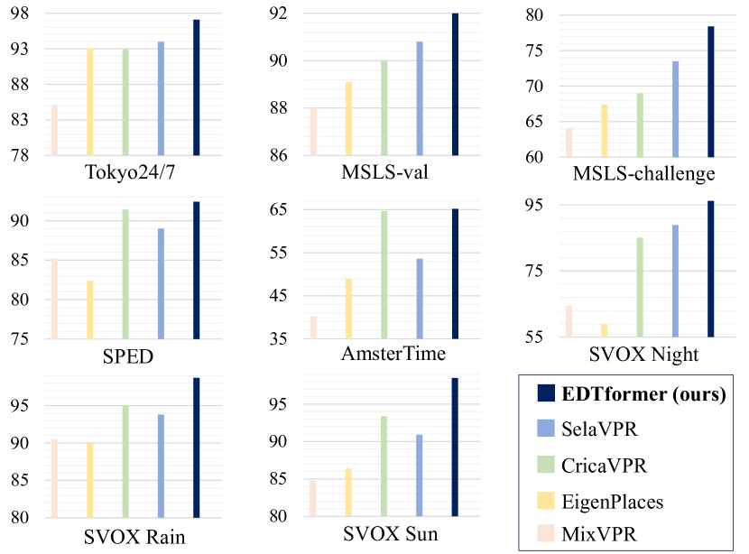
Figure 1: The performance comparison (Recall@1) on multiple benchmark datasets between our method and current state-of-the-art VPR methods, such as MixVPR [33], EngenPlaces [45], CricaVPR [24] and SelaVPR [25]. Our EDTformer consistently shows obvious advantages over other methods in diverse VPR scenarios, including viewpoint variations and condition changes (MSLS [39]), severe lighting changes (Tokyo24/7 [40]), various natural scenes (SPED [60]), place image modality changes (AmsterTime [42]) and varying weather conditions (SVOX [43]).

I Introduction

Visual place recognition, also referred to as visual geo-localization [1], plays an essential role in autonomous driving [2], mobile robot localization [3, 6], augmented reality [8], etc. Therefore, it has attracted considerable interest in the fields of computer vision and robotics over the past decade. However, there still exist various challenges that we have to face in VPR, such as environment variations, viewpoint changes and perceptual aliasing [7, 4]. Addressing these issues while achieving a good accuracy-efficiency trade-off is very difficult but valuable, particularly for single-stage VPR methods that only employ global features.

VPR is generally addressed as a special image retrieval task [9]. Each place image is represented by a global feature, and then the nearest neighbor search is performed in the feature space to obtain the best-matched images of the query. The global features are typically derived from the aggregation of deep features, utilizing some techniques such as NetVLAD [12], GeM [14] pooling or their variants [16, 13, 44]. Unfortunately, such global features usually can not perform well in challenging VPR scenes. To further improve the robustness and retrieval accuracy, recent single-stage VPR research has focused on exploring novel methods to aggregate deep features. For instance, MixVPR [33] incorporates global relationships into each individual feature map through a stack of Feature-Mixer, which just consists of the multi-layer perceptrons (MLPs). CricaVPR [24] proposes a cross-image encoder to calculate the correlation between representations of multiple images in the same batch for robust global features. SALAD [46] redefines the soft assignment of local features in NetVLAD as an optimal transport problem, in which both CNNs and MLPs are fully utilized. BoQ [58] attempts to aggregate features by utilizing the stacked transformer encoders, attention mechanism and multiple sets of learnable queries. However, the transformer decoder structure has not been well explored in the VPR task, despite it being highly renowned in the fields of NLP [35] and semantic segmentation [56, 64, 65, 55] due to its strong capability in capturing contextual dependencies and generating accurate features. We argue that these characteristics of the decoder hold significant potential for addressing various challenges in VPR. To this end, we revisit the transformer decoder and propose an Efficient Decoder Transformer (EDTformer), which can fully utilize the contextual information within the deep features extracted from the backbone, then gradually decode and aggregate the crucial features to output robust and discriminative global representations for the place images.

Moreover, as vision foundation models [20, 22, 21] have demonstrated a remarkable ability for feature extraction, recent VPR studies tend to use a pre-trained foundation model, e.g., DINOv2 [20], as the backbone to extract deep features from the input place images. AnyLoc [23] first applied DINOv2 for VPR without any fine-tuning, making it difficult to fully unleash the capability of DINOv2 for VPR. Then some research [58, 46] began to enhance the performance of DINOv2 in VPR through only fine-tuning the last few encoder blocks of DINOv2. Unfortunately, this process is accompanied by a large number of trainable parameters. Meanwhile, CricaVPR [24] and SelaVPR [25] attempted to apply parameter efficient transfer learning (PETL) methods [26, 49, 50] to adapt DINOv2 for VPR. Specifically, they froze DINOv2 and inserted some additional trainable adapters into each encoder block. However, this approach is efficient only in terms of parameters, not in training time and memory usage, as the gradient computation for the trainable parameters still requires backpropagation through the pre-trained backbone, as shown in Fig. 3 (b). This motivates us to develop a method that can fully strengthen the performance of vision foundation models in the VPR task in a memory- and parameter-efficient way.

In this paper, we revisit the transformer decoder and propose a novel feature aggregation method EDTformer, which can finally generate robust and discriminative global representations for the place images. Without bells and whistles, to fully utilize the rich contextual information within the deep features, our EDTformer adopts a cascade of simplified decoder blocks, which only retain the attention (self-attention and cross-attention) layers and remove the feedforward network for improving the efficiency compared to the standard transformer decoder. By taking deep features as the keys and values, as well as utilizing a set of independent learnable parameters as queries, EDTformer can capture complex contextual relationships encoded in the deep features and progressively decode effective features into the learnable queries to achieve principal feature aggregation. Subsequently, the learnable queries which have contained crucial information are processed through two simple linear layers for dimensionality reduction and further adjustment, producing the final global representation. Meanwhile, we use the foundation model DINOv2 as the backbone in our architecture and develop a memory- and parameter-efficient Low-rank Parallel Adaptation (LoPA) method to adapt DINOv2 for the VPR task. Specifically, we freeze the entire backbone during training and design a tunable lightweight parallel network, which can progressively refine the intermediate features produced by each block of the backbone to output more powerful deep features, resulting in enhancing the performance of the whole model in VPR.

The main contributions of our work are summarized as follows:

(1) We revisit the transformer decoder and propose a novel feature aggregation method EDTformer, by leveraging several stacked simplified decoder blocks, linear projection and a set of learnable queries to fully decode the deep features and finally output a robust and discriminative global representation for global-retrieval-based VPR. This provides a new insight into how to apply the decoder structure for VPR.

(2) We design a Low-Rank Parallel Adaptation method to adapt the foundation model DINOv2 to output enhanced features for boosting performance, which is efficient not only in terms of parameters, but also in training time and memory usage. This can further facilitate the application of the foundation models in resource-constrained VPR scenarios.

(3) Extensive experiments on the benchmark datasets show that our method can outperform the state-of-the-art (SOTA) VPR methods by a considerable margin with less memory usage. The results on multiple datasets which reflect the advantages of our method are shown in Fig. 1.

II Related Work

II-A Visual Place Recognition

In early VPR research, global features were developed by aggregating the hand-crafted local features (e.g., SIFT [28] and SURF [29, 30]), employing some classical aggregation algorithms, such as Bag of Words [31], Fisher Vector [63] and Vector of Locally Aggregated Descriptors (VLAD) [32]. With the great success of deep learning in compute vision tasks, current predominant VPR methods [12, 68, 48, 11, 4, 15, 16, 10, 47, 5, 13, 1, 44, 45, 23, 33, 58, 46, 24, 25] have preferred leveraging large amounts of deep features rather than hand-crafted local features to boost performance. Besides, the traditional aggregation algorithms are gradually replaced by trainable aggregation/pooling layers, such as NetVLAD [12] and GeM pooling [14]. NetVLAD utilizes a trainable generalized VLAD layer to aggregate deep features, typically tending to get a high-dimensional descriptor. In contrast, the Generalized Mean (GeM) pooling is a simple alternative that can produce compact global representations. However, such compact representations usually fall short of delivering satisfactory performance in challenging VPR scenarios. Hence, numerous works [15, 61, 44, 45, 33, 24, 46, 58] proposed various novel training strategies and aggregation algorithms to further improve the global representations for better retrieval accuracy. SFRS [15] proposed self-supervised image-to-region similarities to thoroughly exploit the potential of challenging positive images and their corresponding sub-regions for training a more robust VPR model. CosPlace [44] and EigenPlaces [45] framed the task of VPR training as a classification problem and utilized the San Francisco eXtra Large (SF-XL) dataset to train their VPR models effectively. MixVPR [33] proposed an all-MLP aggregation technique and trained the model utilizing the multi-similarity loss [37] with full supervision. CricaVPR [24] introduced a cross-image correlation-aware representation learning method to enhance the robustness of global features. SALAD [46] reinterpreted the soft assignment of local features in NetVLAD as an optimal transport problem, solving it by using the Sinkhorn algorithm [67]. BoQ [58] utilized multiple sets of queries to capture universal place-specific attributes by utilizing several stacked transformer encoders and attention mechanism. These studies only used global features and achieved a relatively good recognition performance.

In addition, two-stage VPR methods [16, 10, 17, 62], which first search for the top-k candidate images in the database using global features and then re-ranks the candidates based on local features, are also an effective approach to further improve recognition performance. The re-ranking process usually either employs geometric consistency verification or leverages the learnable network to produce dense local features for similarity computation [17, 62, 25]. For instance, DHE-VPR [62] adopted a transformer-based deep homography estimation network to fit homography for fast and learnable geometric verification. SelaVPR [25] introduced a novel hybrid global-local adaptation method and directly used the dense local features in cross-matching for re-ranking. However, the re-ranking is generally time-consuming and demands a huge memory footprint as well as substantial storage space, particularly when dealing with large databases. These shortcomings restrict the applicability of two-stage methods in resource-constrained and large-scale VPR scenarios. Unlike two-stage methods improving performance at a substantial cost, our proposed method efficiently uses the decoder to aggregate deep features and directly produce highly robust and discriminative global representations for global-retrieval-based VPR.

II-B Transformer Decoder Architecture

Since the success of the transformer [35] in NLP, the scope of transformer decoder has expanded to various computer vision tasks [18, 19, 54, 66, 65]. For instance, DETR [54] was the first to apply the transformer decoder for object detection and used multiple learnable object queries to capture the information of target objects, finally outputting a set of predictions in parallel. SenFormer [64], MaskFormer [65] and Mask2Former [66] used the stacked transformer decoders to generate segmentation masks by learning query sets, which can refine multi-scales features extracted from the backbone and denote some possible segmentation regions. IAA-LQ [59] used a standard transformer decoder to estimate the aesthetics of images. Different from them, we first simplify the structure of the transformer decoder by removing the feedforward network to get a higher efficiency. Additionally, the purpose of using learnable queries is distinct. Our learnable queries primarily are used to aggregate global contextual information from deep features of the place image under the action of our EDTformer, rather than focusing on specific pixels or pixel blocks/objects in the image.

II-C Parameter Efficient Transfer Learning

The vision foundation models [20, 21, 22] trained on huge quantities of data, such as DINOv2 (trained on the large-scale curated LVD-142M dataset with the self-supervised strategy), possess the ability to extract powerful features from the input images and have achieved remarkable results on various downstream vision tasks. In order to reduce the number of training parameters while maintaining the strong capability of these foundation models, the PETL methods [26, 49, 27, 50] have been proposed and are widely applied in many areas, including the VPR field. For example, CricaVPR [24] enhanced the performance of DINOv2 in VPR by introducing multi-scale convolution adapters. SelaVPR [25] inserted the vanilla adapters into DINOv2 to achieve a hybrid global-local adaptation to produce both global and local features for the VPR task. By only tuning the built-in lightweight adapters without adjustment to the frozen pre-trained model, they are both efficient in terms of parameters. Nevertheless, the memory overhead during training is primarily dominated by the activations, not only parameters, which means that parameter efficiency is not equivalent to memory efficiency [53]. Unlike them, we design a Low-Rank Parallel Adaptation method to fully unleash the capability of the pre-trained vision foundation model without inserting any parameter into it, which is both parameter- and memory-efficient.

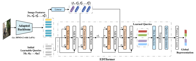
Figure 2: The pipeline to produce the robust and discriminative global representation for single-stage VPR. Firstly, the backbone with Low-rank Parallel Adaptation (i.e., DINOv2 with LoPA) is employed to extract powerful deep features of the input image. Next, the features undergo a linear transformation and are fed into each cross-attention layer as the keys and values. Additionally, we initial a set of learnable queries as the input queries for the first self-attention layer. After passing through $L$ decoder blocks, we can obtain the learned queries which have aggregated the crucial contextual features. Then we use two fully connected layers: one for dimensionality reduction and the other for further information aggregation by adjusting the number of queries. Finally, the output features are flattened and L2-normalized as the global representation of the place image.

III Methodology

In this section, we first briefly introduce our backbone for feature extraction. Next, we propose the EDTformer to achieve feature aggregation efficiently. Then we introduce the LoPA to adapt the foundation model to provide more powerful features for EDTformer, improving the performance of the whole model in a memory- and parameter-efficient way. Finally, we describe the training strategy in our experiments.

III-A Feature Extraction

In this work, we adopt the vision foundation DINOv2 as the backbone, which is based on Vision Transformer (ViT) [34]. To process the input image $I\in\mathbb{R}^{w\times h\times c}$, ViT first divides the image into $p\times p$ non-overlapping small patches, and then linearly projects them into $d$-dimensional tokens $x_{p}\in\mathbb{R}^{N\times d}$ ($N=p\times p$). Meanwhile, a learnable class token is prepended to $x_{p}$ to obtain $x_{0}=[x_{class},x_{p}]\in\mathbb{R}^{(N+1)\times d}$. Subsequently, position embeddings are added to $x_{p}$ to preserve positional information, resulting in $z_{0}$, which will be processed by a series of repeated transformer encoder blocks to extract features. A transformer encoder block mainly consists of the Multi-Head Attention (MHA) layer, the Multi-Layer Perceptron (MLP), and the LayerNormalization (LN), as shown in Fig. 3 (a). The token sequence $z_{l-1}$ goes through the transformer encoder block and produces $z_{l}$, which can be formulated as

$$z^{\prime}_{l} =MHA(LN(z_{l-1}))+z_{l-1},$$ (1)

$$z_{l} =MLP(LN(z^{\prime}_{l}))+z^{\prime}_{l},$$

where $z_{l-1}$ and $z_{l}$ are the outputs of the $(l-1)$-th and $l$-th transformer encoder blocks, respectively. Based on these extracted features, we will further introduce how to adapt DINOv2 efficiently using LoPA in the subsection III-C.

III-B EDTformer

The EDTformer primarily relies on MHA mechanism, so we provide a detailed introduction. The MHA first maps the input sequence into queries Q, keys K, and values V h times with different learnable linear projections. Then, the attention between Q, K, and V is computed through scaled dot-product [35], formulated as

$$Attn(Q,K,V)=softmax\big{(}QK^{\top}/\sqrt{d}\big{)}V.$$ (2)

On each of these projected versions of queries, keys and values, we then perform the attention function in parallel, yielding h output values. These are concatenated and once again projected ($W_{O}$), resulting in the final values, which can be expressed as

$$MHA(Q,K,V) =Concat(head_{1},\dots,head_{h})W_{O},$$ (3)

$$head_{i} =Attn(Q_{i},K_{i},V_{i}).$$

Notably, the self-attention layer uses the same feature as query, key and value, whereas the cross-attention layer uses one feature as query and the other feature as key and value. We will use both of them to construct EDTformer to obtain robust and discriminative global features.

We design a simple yet powerful pipeline to produce promising global features as shown in Fig. 2. For the deep features $\mathcal{X}:\{x_{c},x^{1}_{p},x^{2}_{p},\ldots,x^{N}_{p}\}\in\mathbb{R}^{(N+1)\times d}$ output by the adapted backbone (i.e., DINOv2 with LoPA), we apply a linear projection to $\mathcal{X}$ for feature transformation and information transfer to obtain features $\mathcal{F}:\{f_{c},f^{1}_{p},f^{2}_{p},\ldots,f^{N}_{p}\}\in\mathbb{R}^{(N+1)\times d}$, which can be formulated as

$$\mathcal{F}=W_{1}\mathcal{X}+b_{1}.$$ (4)

The proposed EDTformer adopts a pure decoder structure, which utilizes the simplified decoder block and a fixed set of learnable queries. Different from the standard transformer decoder, our simplified decoder only consists of a self-attention layer and a cross-attention layer without the feedforward network (FFN) for higher efficiency. For the first self-attention layer, the input vector Q, K, V come from a set of learnable queries, denoted as $\mathcal{Q}:\{q_{1},q_{2},\dots,q_{M}\}\in\mathbb{R}^{M\times d}$ ($M<N$). These queries are trainable parameters of the model and independent of the input features. Notably, for the subsequent self-attention layers, the input comes from the output of the preceding decoder block. Through the self-attention operation, these queries can conduct internal information interaction to reduce redundancy and highlight the essential parts. Unlike the self-attention layer, the input of the cross-attention layer comes from two sources: Q is derived from the output of the self-attention layer, while K and V are the previous features $\mathcal{F}$. By the cross-attention mechanism, the module can dynamically transfer and aggregate effective contextual information within $\mathcal{F}$ to the learnable queries $\mathcal{Q}$ according to the cross-attention weights between them. To fully make use of $\mathcal{F}$, we adopt $L$ decoder blocks in a cascading way to decode layer by layer, thereby the initial learnable queries $\mathcal{Q}$ gradually result in the learned queries $\mathcal{O}_{L}:\{o_{1},o_{2},\dots,o_{M}\}\in\mathbb{R}^{M\times d}$. The internal process of each decoder block can be denoted as

$$\mathcal{Q}_{i}=LN(MHA(\mathcal{O}_{i-1},\mathcal{O}_{i-1},\mathcal{O}_{i-1})+\mathcal{O}_{i-1}),$$ (5)

$$\mathcal{O}_{i}=LN(MHA(\mathcal{Q}_{i},\mathcal{F},\mathcal{F})+\mathcal{Q}_{i}),$$ (6)

where $\mathcal{Q}_{i}$ and $\mathcal{O}_{i}$ respectively are the outputs of the $i$-th self-attention layer and cross-attention layer. Notably, the $\mathcal{O}_{0}$ is the initial learnable queries $\mathcal{Q}$.

Subsequently, we utilize two fully connected layers: the first to reduce the dimensionality of learned queries, and the second to adjust the number of queries for further feature aggregation, formulated as

$$\text{Output}=W_{3}(W_{2}\mathcal{O}_{L}+b_{2})^{T}+b_{3}.$$ (7)

Finally, we flatten the output features and employ the L2-normalization to obtain the robust and discriminative global representation of the input place image.

It is worth noting that the latest work BoQ [58] and our EDTformer both utilize the learnable queries, but the architectures are completely different. BoQ uses multiple stacked encoders to deal with the deep features extracted from the backbone and applies separate attention mechanism, as well as multiple sets of independent queries to individually learn the output of each encoder. In contrast, we discard the encoder blocks and first attempt to directly utilize a purely decoder-based structure with only a set of queries to achieve the feature aggregation in VPR, which is simpler and more efficient.

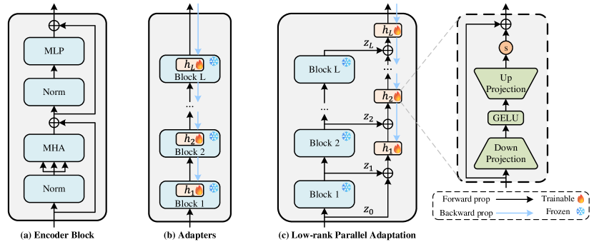
Figure 3: Illustration of our Low-rank Parallel Adaptation method. (a) is a standard transformer encoder block in ViT. (b) is the popular PETL method based on adapters, which usually inserts the trainable adapters into the encoder blocks of the frozen backbone. (c) is the proposed LoPA method. We design it as a separate and lightweight network so that backpropagation does not pass through the frozen backbone to greatly reduce memory usage during training.

III-C Low-rank Parallel Adaptation

The foundation model DINOv2 recently has become a popular backbone for feature extraction in VPR, generally accompanied by a fine-tuning/adaptation for better performance. CricaVPR [24] and SelaVPR [25] have used the PETL methods (i.e., inserting tunable adapters into the frozen encoder blocks) to adapt DINOv2, as shown in Fig. 3 (b). However, they are efficient only in terms of parameters, not in training time and memory usage. Here, we conduct a simple theoretical derivation to explain this point. For a network with $L$ blocks, each having output ${z}_{i}$, a large number of frozen parameters $\theta_{i}$ and a few trainable parameters $\psi_{i}$, our goal is to minimize a loss function, $\mathcal{L}$ based on stochastic gradient descent. Concretely, to update $\psi_{i}$ during backpropagation, we first need to compute $\frac{\partial\mathcal{L}}{\partial\psi_{i}}$ via the chain rule as follows

$$\frac{\partial\mathcal{L}}{\partial\psi_{i}}=\underbrace{\frac{\partial\mathcal{L}}{\partial z_{L}}\frac{\partial z_{L}}{\partial z_{L-1}}\cdots\frac{\partial z_{i+1}}{\partial z_{i}}}_{\text{intermediate activations}}\frac{\partial z_{i}}{\partial\psi_{i}}=\frac{\partial\mathcal{L}}{\partial z_{i}}\frac{\partial z_{i}}{\partial\psi_{i}}.$$ (8)

Although $\frac{\partial z_{i}}{\partial\psi_{i}}$ can be directly computed, in order to calculate $\frac{\partial\mathcal{L}}{\partial z_{i}}$, it is inevitable to compute gradients about the intermediate activations, as shown in Eq. (8), which can incur huge memory overhead and additional running time.

To tackle the above issue, we propose the Low-rank Parallel Adaptation method inspired by previous studies [51, 52]. Instead of inserting tunable parameters inside the backbone, we design a parallel network that does not require backpropagation gradients through the frozen backbone during training as shown in Fig. 3 (c). It is a lightweight and separate network, which directly takes the intermediate features from the backbone as inputs and refines them progressively to produce more accurate representations.

Concretely, our backbone DINOv2 consists of a patch embedding block and $L$ encoder blocks, and therefore $L+1$ outputs $z_{0},z_{1},z_{2}...,z_{L}$, each composed of $N+1$ tokens with a dimensionality of $d$, so $z_{i}\in\mathbb{R}^{(N+1)\times d}$. We learn parallel adaptation functions, $h$, which operate on these intermediate features to refine them. We denote the outputs of our adaptation functions as $y_{i}$ where $i$ denotes the function index. The whole process can be formulated as

$$y_{i}=\begin{cases}h_{i}(z_{i-1}+z_{i})&\text{if }i=1,\\ h_{i}(y_{i-1}+z_{i})&\text{otherwise}.\end{cases}$$ (9)

To be more efficient, we design our adaptation function $h$ in a low-rank structure with few parameters. Specially, $h$ consists of a down-projection, $W_{d}:\mathbb{R}^{d}\rightarrow\mathbb{R}^{r}$, a GeLU non-linearity activation $\sigma(\cdot)$ [57], and an up-projection, $W_{u}:\mathbb{R}^{r}\rightarrow\mathbb{R}^{d}$ with a skip-connection, where $r\ll d$. As in [25, 24, 52], we also add a scaling factor $s$, meaning that our adaptation function can be denoted as

$$h(x)=sW_{u}\sigma(W_{d}x)+x.$$ (10)

III-D Training Strategy

The proposed model is trained on the GSV-Cities [36] dataset following its standard framework. GSV-Cities contains 560k images with highly accurate labels depicting 67k different places. We apply the multi-similarity (MS) loss [37] function with an online hard mining strategy. The MS loss is formulated as

$$\mathcal{L}_{MS} =\frac{1}{B}\sum_{q=1}^{B}\left\{\frac{1}{\alpha}\log\left[1+\sum_{p\in\mathcal{P}_{q}}e^{-\alpha(S_{qp}-\lambda)}\right]\right.$$ (11)

$$\quad\left.+\frac{1}{\beta}\log\left[1+\sum_{n\in\mathcal{N}_{q}}e^{\beta(S_{qn}-\lambda)}\right]\right\},$$

where for each query image $I_{q}$ in a batch, $\mathcal{P}_{q}$ represents the set of indices {$p$} which align with the positive samples for $I_{q}$, and $\mathcal{N}_{q}$ represents the set of indices {$n$} which align with the negative samples for $I_{q}$. $S_{qp}$ and $S_{qn}$ respectively represent the cosine similarity of a positive sample pair $\{I_{q},I_{p}\}$ and a negative sample pair $\{I_{q},I_{n}\}$. The remaining variables $\alpha$, $\beta$ and $\lambda$ are three sets of hyperparameters.

IV Experiments

IV-A Datasets and Evaluation Metrics

To demonstrate the effectiveness of our method, we conduct the experiments on multiple benchmark datasets, which present a diverse set of challenges encountered in the real world. Table I provides a concise summary of these benchmark datasets. Pitts30k [38], extracted from Google Street View, shows significant changes in viewpoint. MSLS [39] is collected from 30 major cities across six continents over nine years period, covering all seasons and encompassing diverse weather, cameras, daylight conditions, and structural settings. Tokyo24/7 [40] presents severe lighting (day/night) variations. SPED [60] is collected from surveillance cameras and encompasses a diverse array of natural scenes. Nordland [41] is captured using a front-mounted train camera, spanning all four seasons. We use the winter images as queries and summer images as database followed by previous work [1, 45, 24]. AmsterTime [42] exhibits substantial image modality variations, using historical grayscale images as queries and contemporary color images as database. SVOX [43] is a cross-domain VPR dataset gathered under diverse weather and lighting conditions. We primarily utilize the three most challenging query subsets: SVOX Night, SVOX Rain and SVOX Sun.

We use the Recall@N (R@N) in the experiments for performance evaluation, which is defined as the percentage of query images for which at least one of the top-N candidates falls within a threshold of ground truth. Consistent with previous work [38, 39, 40, 24, 45], we set the threshold to 25 meters and $40^{\circ}\text{angle}$ for MSLS, 25 meters for Pitts30k, Tokyo24/7, SPED and SVOX, $\pm 10$ frames for Nordland, special counterpart for AmsterTime.

TABLE I: Brief summary of the benchmark datasets in our experiments.

Dataset	Description	Number
		Database	Queries
Pitts30k [38]	viewpoint changes	10,000	6,816
MSLS-val [39]	urban, suburban	18,871	740
MSLS-challenge [39]	long-term	38,770	27,092
Tokyo24/7 [40]	illumination changes	75,984	315
SPED [60]	various scenes	607	607
Nordland [41]	season variants	27,592	27,592
Amstertime [42]	domain variants	1,231	1,231
SVOX [43]	condition variations	17,166	14,278

IV-B Implementation Details

We use DINOv2-base as the backbone and conduct experiments on NVIDIA GeForce RTX 4090 GPUs using PyTorch. The backbone is completely frozen and only LoPA is trainable to refine the features from the backbone progressively. The low rank $r$ in LoPA is set to 4 and the scaling factor $s$ in Eq. (10) is set to 0.5. We apply two stacked simplified decoder blocks for a trade-off between accuracy and efficiency, and leverage 64 queries to fully learn the effective features. Finally, the model outputs a 4096-dim global descriptor. We set the hyperparameters $\alpha=1$, $\beta=50$, $\lambda=0$ in Eq. (11) and margin = 0.1 in online mining, as in previous work [33, 24, 58]. We train our model using the Adam optimizer with the initial learning rate set as 0.0001 and multiplied by 0.7 after every 3 epochs. Each training batch consists of 72 places, with 4 images per place, totaling 288 images. The resolution of the input image is $224\times 224$ during training ($322\times 322$ in reference). We train the model for 15 epochs in total.

TABLE II: Comparison to state-of-the-art methods on benchmark datasets. The best is highlighted in bold and the second is underlined. $\dagger$ CricaVPR utilizes a cross-image encoder to correlate multiple images from the same place at once in inference to get a better performance, so it is not included in the comparison with other methods. We additionally show the results (CricaVPR-1) of single query image in inference. ${\ddagger}$ We reproduce the results of BoQ by strictly following its training pipeline, except for keeping the same image size for both training ($224\times 224$) and inference ($322\times 322$) as our method.

Method	Dim	MSLS-challenge			Tokyo24/7			MSLS-val			SPED			Pitts30k
		R@1	R@5	R@10	R@1	R@5	R@10	R@1	R@5	R@10	R@1	R@5	R@10	R@1	R@5	R@10
NetVLAD [12]	32768	35.1	47.4	51.7	60.6	68.9	74.6	53.1	66.5	71.1	70.2	84.5	89.5	81.9	91.2	93.7
SRFS [15]	4096	41.6	52.0	56.3	81.0	88.3	92.4	69.2	80.3	83.1	80.2	92.6	95.4	89.4	94.7	95.9
CosPlace [44]	512	61.4	72.0	76.6	81.9	90.2	92.7	82.8	89.7	92.0	75.5	87.0	89.6	88.4	94.5	95.7
MixVPR [33]	4096	64.0	75.9	80.6	85.1	91.7	94.3	88.0	92.7	94.6	85.2	92.1	94.6	91.5	95.5	96.3
EigenPlaces [45]	2048	67.4	77.1	81.7	93.0	96.2	97.5	89.1	93.8	95.0	82.4	91.4	94.7	92.5	96.8	97.6
CricaVPR† [24]	4096	69.0	82.1	85.7	93.0	97.5	98.1	90.0	95.4	96.4	91.4	95.6	96.7	94.9†	97.3†	98.2†
CricaVPR-1 [24]	4096	66.9	79.3	82.3	89.5	94.6	96.2	88.5	95.1	95.7	87.3	92.9	94.7	91.6	95.7	96.9
BoQ‡ [58]	12288	75.9	87.4	90.3	95.2	97.8	98.1	91.2	95.7	96.4	88.6	95.2	96.2	91.9	95.9	97.2
SALAD [46]	8448	75.0	88.8	91.3	94.6	97.5	97.8	92.2	96.4	97.0	92.1	96.2	96.6	92.5	96.4	97.5
SelaVPR (global) [25]	1024	69.6	86.9	90.1	81.9	94.9	96.5	87.7	95.8	96.6	83.9	91.3	93.6	90.2	96.1	97.1
Patch-NetVLAD [16]	/	48.1	57.6	60.5	86.0	88.6	90.5	79.5	86.2	87.7	87.2	93.1	94.2	88.7	94.5	95.9
$R^{2}$Former [17]	/	73.0	85.9	88.8	88.6	91.4	91.7	89.7	95.0	96.2	67.6	75.8	78.4	91.1	95.2	96.3
SelaVPR [25]	/	73.5	87.5	90.6	94.0	96.8	97.5	90.8	96.4	97.2	89.0	94.6	96.4	92.8	96.8	97.7
EDTformer (ours)	4096	78.4	89.8	91.9	97.1	98.1	98.4	92.0	96.6	97.2	92.4	95.9	96.9	93.4	97.0	97.9

TABLE III: Comparison to SOTA methods on more challenging datasets. The best is highlighted in bold and the second is underlined. ${\ddagger}$ We reproduce the results of BoQ by strictly following its training pipeline, except for keeping the same image size for both training ($224\times 224$) and inference ($322\times 322$) as our method.

Method	Nordland			AmsterTime			SVOX Night			SVOX Rain			SVOX Sun
	R@1	R@5	R@10	R@1	R@5	R@10	R@1	R@5	R@10	R@1	R@5	R@10	R@1	R@5	R@10
SFRS [15]	16.0	24.1	28.7	29.7	48.5	55.6	28.6	40.6	46.4	69.7	81.5	84.6	54.8	68.3	74.1
CosPlace [44]	58.5	73.7	79.4	38.7	61.3	67.3	44.8	63.5	70.0	85.2	91.7	93.8	67.3	79.2	83.8
MixVPR [33]	76.2	86.9	90.3	40.2	59.1	64.6	64.4	79.2	83.1	91.5	97.2	98.1	84.8	93.2	94.7
EigenPlaces [45]	71.2	83.8	88.1	48.9	69.5	76.0	58.9	76.9	82.6	90.0	96.4	98.0	86.4	95.0	96.4
CricaVPR-1 [24]	79.4	90.1	93.3	49.4	70.3	76.7	76.8	88.0	92.3	93.5	98.5	99.0	87.8	97.2	97.9
BoQ‡ [58]	85.0	93.5	95.7	52.8	74.2	80.2	95.8	99.2	99.3	97.8	99.5	99.7	97.8	99.4	99.4
SelaVPR [46]	87.3	93.8	95.6	53.6	72.8	78.1	88.9	95.7	97.3	93.8	98.4	98.9	90.9	96.0	96.8
EDTformer (Ours)	88.3	95.3	97.0	65.2	85.0	89.0	96.2	98.7	99.3	98.7	99.8	99.8	98.5	99.5	99.8

IV-C Comparison with State-of-the-art Methods

In this section, we compare our proposed method with a wide range of existing SOTA VPR algorithms, including eight single-stage VPR methods using global features for direct retrieval: NetVLAD [12], SFRS [15], CosPlace [44], MixVPR [33], EigenPlaces [45], CricaVPR [24] and BoQ [58], as well as three superior two-stage VPR methods: Patch-NetVLAD [16], $R^{2}$Former [17] and SelaVPR [25]. Notably, our work uses the same training dataset as MixVPR, CricaVPR, SALAD and BoQ, i.e., GSV-Cities. Additionally, the latest works CricaVPR, SALAD, BoQ and SelaVPR all leverage the foundation model DINOv2 as the backbone (SelaVPR using DINOv2-large, while others using DINOv2-base) and achieve the SOTA performance on multiple benchmarks. Thus, we follow them and apply the DINOv2-base. Table II shows the quantitative results on MSLS, Tokyo24/7, SPED and Pitts30k. Our method achieves the best R@1/R@5/R@10 performance on almost all datasets.

Results analysis. CricaVPR, SALAD, BoQ, SelaVPR and our method all achieve superior performance on these datasets. Especially on Tokyo24/7, which shows severe illumination changes, CricaVPR, SALAD, BoQ and SelaVPR achieve 93.0% R@1, 94.6% R@1, 95.2% R@1 and 94.0% R@1 respectively. However, our method consistently improves performance on Tokyo24/7, achieving an incredible 97.1% R@1. This improvement stems from the robust and discriminative global descriptors generated by our model. The MSLS dataset is highly challenging, covering different seasons, weather and illumination conditions, various camera types and viewpoints, as well as different levels of dynamic objects presented in the scenes. Nevertheless, our method achieves 78.4% R@1, 89.8% R@5 and 91.9% R@10 on MSLS-challenge, showing significant advantages and outperforming other global-retrieval-based methods and two-stage methods by a considerable margin. Although our method achieves 92.0% R@1 on MSLS-val, 0.2% lower than SALAD, the dimensionality of our global descriptors is less than half that of SALAD. This indicates that our global descriptors can require less storage space and achieve a higher retrieval efficiency. In addition, we also get an overall better performance on the SPED dataset, demonstrating the high robustness of our method to handle various place images concerning natural scenes. On the Pitts30k dataset, which shows severe viewpoint changes, EDTformer outperforms all other methods but is slightly behind CricaVPR. This is because CricaVPR uses the cross-image encoder to combine the information of multiple query images from the same place in a batch at once in inference. As the number of query images in the batch decreases, especially when it becomes 1, the performance of CricaVPR drops significantly, as shown in Table II CricaVPR-1.

To further evaluate the generalization of our method in some extreme scenarios, we conduct extensive experiments on other challenging datasets: Nordland, AmsterTime, SVOX Night, SVOX Rain and SVOX Sun. The results shown in Table III demonstrate the powerful capability of our method to effectively tackle the VPR task in difficult scenes. On the Nordland dataset, which exhibits significant variations in seasons and illumination, our EDTformer gets the best performance, even outperforming the two-stage SelaVPR. Additionally, our method surpasses other methods on the AmsterTime dataset by a large margin. Specifically, it outperforms the second by 11.6%, 10.8% and 8.8% on R@1/R@5/R@10 respectively. This implies the high robustness of our method to handle image modality variations in the datasets both containing grayscale and colorful images. On the SVOX Night, SVOX Rain and SVOX Sun datasets, our EDTformer achieves a relatively perfect performance (e.g., 98.7% R@1, 99.8% R@5 and 99.8% R@10 on SVOX Rain), which shows that it can be well applied to these special scenarios. In summary, the results on these challenging datasets further highlight the robust generalization capability of our model.

Moreover, our method also exhibits an advantage in terms of efficiency. Fig. 4 exhibits the R@1 performance on the Pitts30k dataset and the inference time of a single image about six global-retrieval-based methods, including SFRS, MixVPR, SALAD, BoQ, SelaVPR (global) and our EDTformer. MixVPR uses the CNN model (ResNet-50) as the backbone and proposes a feature mixing method to get global descriptors, which achieves the fastest inference speed. Although SFRS also leverages the CNN model (VGG-16), it applies PCA to reduce the dimensionality of the global descriptors, which is time-consuming. The other methods are all based on the vision foundation models. Specifically, SelaVPR (global) adopts DINOv2-large as the backbone, resulting in the slowest inference speed (16.95 ms). Among SALAD, BoQ and our EDTformer, all of which use DINOv2-base as the backbone, our method achieves the fastest inference speed (9.16 ms). In addition, we also provide the training memory consumption and training time per epoch for the three methods, as shown in Table. IV. Our training speed is approximately 15% faster and the training memory usage is much less than half of theirs. In summary, our method is efficient both in training and inference while achieving a superior recognition performance.

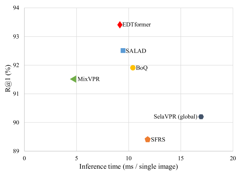
Figure 4: The R@1 and inference time comparison of different single-stage methods on Pitts30k. We measure the inference time on an NVIDIA GeForce RTX 4090 GPU.

TABLE IV: The comparison of SALAD, BoQ and our EDTformer in training memory usage and training time. We train the three models on GSV-Cities with batch size set to 36 and consistently measure the metrics on an NVIDIA GeForce RTX 4090 GPU.

Metric	SALAD	BoQ	EDTformer
Training Memory Usage (GB)	14.81	15.21	5.72
Training Time (min / epoch)	11.21	10.67	8.77

IV-D Ablation Studies

In this section, we first conduct a series of ablation experiments to demonstrate the effectiveness of our proposed EDTformer and LoPA. Subsequently, we further explore the impact of some design details about the EDTformer and LoPA. Notably, we consistently use the GSV-Cities dataset with the multi-similarity loss for training in the ablation experiments. Unless otherwise specified, the dimensionality of the global features produced by our method is 4096.

TABLE V: Ablation on different aggregation methods. The dimensionality of global descriptors is reported.

Method	Dim	MSLS-val		SPED		Pitts30k		Nordland
		R@1	R@5	R@1	R@5	R@1	R@5	R@1	R@5
GeM	768	85.7	94.6	76.1	88.5	88.5	94.4	32.3	47.1
GeM-linear	4096	87.3	93.6	86.0	93.6	91.5	95.9	63.0	77.3
NetVLAD	24576	89.7	95.5	88.8	95.1	92.0	96.5	71.7	84.8
NetVLAD (PCA)	4096	89.3	95.3	87.5	93.9	92.0	96.3	71.7	84.6
Conv-AP	4096	72.7	80.9	82.0	92.1	89.5	94.8	50.8	67.6
MixVPR	4096	89.2	94.6	89.8	94.4	91.1	95.3	79.4	89.2
BoQ	12288	91.5	96.5	91.1	95.7	93.1	96.6	83.8	92.2
EDTformer	4096	92.0	96.6	92.4	95.9	93.4	97.0	88.3	95.3
EDTformer	2048	91.4	96.6	90.6	95.7	93.4	96.7	82.3	91.9
EDTformer	1024	91.4	95.7	90.6	96.0	92.5	96.6	78.6	89.8
EDTformer	512	90.1	95.7	89.3	94.9	91.7	96.0	71.1	84.6

Effect of EDTformer. To validate the effectiveness of the proposed EDTformer, we compare it with current common aggregation methods, including GeM [14], NetVLAD [12], Conv-AP [36], MixVPR [33] and BoQ [58] (related to our method). The “GeM-linear” represents the use of the GeM aggregator, followed by a linear layer to adjust the dimensionality of the descriptors. Likewise, “NetVLAD-PCA” implies that a PCA layer is integrated after the NetVLAD aggregator to perform dimensionality reduction. To ensure the fairness of the experiments, we consistently use DINOv2-base as the backbone with LoPA (rank set to 4) for feature extraction. The results are presented in Table V. When the dimensionality of global descriptors is the same (4096-dim), our EDTformer achieves highly competitive performance and outperforms some other aggregators (e.g., GeM, NetVLAD, Conv-AP and MixVPR) by a large margin. Although BoQ also achieves outstanding results, it is worth mentioning that the dimensionality of the global descriptors (12288-dim) produced by BoQ is more than three times of that of our global representations (4096-dim). In this case, our method still achieves a better performance than BoQ, especially on the Nordland dataset (obtaining an improvement of 4.5% in R@1). Moreover, we simultaneously present the recognition performance of our global descriptors with varying dimensions (achieved by only adjusting the last linear layer in our pipeline). As the dimensionality of the descriptors decreases, the overall performance gradually declines. However, the 512-dim descriptors can still achieve an impressive 90.1% R@1 on MSLS-val, 89.3% R@1 on SPED, 91.7% R@1 on Pitts30k and 71.1% R@1 on Nordland, surpassing the performance of the 768-dim descriptors outputed by GeM and remaining competitive against some SOTA methods such as SFRS [15], CosPlace [44] and EigenPlace [45]. Therefore, our EDTformer is also well-suited for some VPR scenarios that urgently require low-dimensional descriptors.

TABLE VI: Ablation on different fine-tuning/adaptation methods. “PartialTune-2” and “PartialTune-4” respectively denote only training the last 2 and 4 encoder blocks of DINOv2. “MCAdapter” is the abbreviation of MultiConvAdapter. The trainable parameters introduced by different methods are reported. We use an NVIDIA A800 GPU to measure the training memory usage with batch size set to 72.

Method	Params $\downarrow$	Memory $\downarrow$	MSLS-val		SPED		Nordland
	(M)	(GB)	R@1	R@5	R@1	R@5	R@1	R@5
Frozen	0	8.35	90.8	96.1	90.1	95.6	74.3	86.3
PartialTuned-2	14.18	15.54	90.8	95.1	89.0	95.4	79.3	89.6
PartialTuned-4	28.36	23.63	91.1	95.4	86.0	92.9	74.1	85.5
FullTuned	86.58	54.40	88.0	95.4	83.0	91.6	72.3	84.7
Adapter [25]	14.18	40.07	91.1	96.2	89.6	94.6	88.8	95.6
MCAdapter [24]	9.16	39.30	91.8	96.4	90.9	95.1	86.5	93.8
LoPA (ours)	0.08	10.09	92.0	96.6	92.4	95.9	88.3	95.3

Effect of LoPA. Next, to verify the effectiveness and efficiency of the proposed LoPA method, we compare it with other popular fine-tuning/adaptation methods, including PartialTuned (only fine-tuning the last few blocks of the backbone while keeping the others frozen), FullTuned (training the entire backbone), Adapter (as implemented in SelaVPR [25]) and MultiConvAdapter (as implemented in CricaVPR [24]). We use DINOv2-base as the backbone and set the frozen backbone without any adjustment as baseline. Besides, we consistently use our EDTformer as the aggregator. The results are presented in Table VI. In terms of efficiency, LoPA is an extremely lightweight network, solely introducing 0.08M trainable parameters, fewer than 1% of the parameters compared to other methods. In addition, compared to the frozen baseline, it only adds 1.74GB training memory, 10 times less than the PETL methods used in SelaVPR [25] and CricaVPR [24]. Amazingly, it saves over 40GB training memory usage compared to FullTuned. This demonstrates that LoPA is both parameter-efficient and memory-efficient, which makes it highly appropriate for VPR scenarios with constrained computational resources. In terms of accuracy, LoPA also significantly improves the performance of DINOv2 in VPR, while other methods result in minimal improvements or even a decline. Specifically, without any adjustment to DINOv2, our EDTformer remains competitive against some SOTA methods, such as MixVPR [33] and EigenPlaces [45]. Building on this, the LoPA further improves the baseline with 1.2%, 14.0% and 2.3% absolute R@1 on MSLS-val, Nordland and SPED. In contrary, PartialTuned yields minimal performance improvement on MSLS-val and Nordland. FullTuned, on the other hand, results in an overall performance decline. The PETL methods, i.e., Adapter and MultiConvAdapter, improve the recognition performance of the model on the MSLS-val and Nordland datasets. Yet these methods all lead to a decrease in R@5 on SPED. Comprehensively, the features output by DINOv2 with LoPA are more suitable for the sequent EDTformer to form the global representation, thereby achieving better performance at a minimal cost.

TABLE VII: Ablation on the number of decoder blocks. The parameters of decoder blocks are reported. We consistently use DINOv2-base as the backbone with LoPA (rank set to 4) and leverage 64 queries as one of the inputs for EDTformer.

Number	Params	MSLS-val		SPED		Pitts30k		Nordland
	(M)	R@1	R@5	R@1	R@5	R@1	R@5	R@1	R@5
1	4.73	91.8	96.6	92.1	96.0	93.1	96.6	78.4	88.4
2	9.46	92.0	96.6	92.4	95.9	93.4	97.0	88.3	95.3
3	14.18	92.6	96.2	91.3	96.4	93.0	96.7	86.9	94.6
4	18.91	91.9	96.9	90.9	95.9	93.1	96.9	88.2	95.3
6	28.37	91.8	96.2	89.3	94.4	92.7	96.5	84.0	92.9

TABLE VIII: Ablation on the number of learnable queries. We consistently use DINOv2-base as the backbone with LoPA (rank set to 4). The overall performance is best with 64 queries.

Number of learnable queries	MSLS-val		SPED		Pitts30k		Nordland
	R@1	R@5	R@1	R@5	R@1	R@5	R@1	R@5
8	91.1	96.5	91.4	95.9	92.8	96.7	77.4	88.5
16	92.2	96.5	90.8	95.9	92.7	96.7	80.9	91.0
32	91.5	96.2	91.4	96.0	93.2	96.7	86.1	94.3
64	92.0	96.6	92.4	95.9	93.4	97.0	88.3	95.3
96	92.6	96.5	92.3	96.4	93.0	97.0	85.4	94.0

Effect of the number of decoder blocks. To evaluate the impact of the number of decoder blocks used in our EDTformer architecture, we conduct the ablation experiments by changing the number of decoder blocks. The results, as shown in VII, demonstrate that even using one decoder block, EDTformer can still get a competitive performance compared to some SOTA methods, such as MixVPR [33], CricaVPR [24] and SelaVPR [25]. The overall best performance is achieved by constructing the EDTformer with two stacked decoder blocks, which can fully decode and aggregate the crucial contextual information from the deep features. In contrast, further increasing the number of decoders (e.g., 3 and 4) provides very limited improvement and even slightly degrades the overall performance. Besides, there is an obvious drop in recognition accuracy when the number of decoder blocks increases to 6. Moreover, the increase in parameters and memory consumption caused by stacking more decoder blocks is also a non-negligible issue. For a better trade-off between efficiency and accuracy, using 2 decoder blocks to construct EDTformer is a good choice.

Effect of the number of learnable queries. In this part, we conduct the ablation studies on the number of learnable queries. The results are presented in Table VIII. Since the learnable queries are an essential input of EDTformer, their quantity affects the quality of the global features. We can observe that the overall performance of the model improves as the number of learnable queries increases. However, when the number of queries becomes too large, it not only introduces an additional computational burden but also is unable to sufficiently learn effective features, which hinders the generation of a robust and discriminative global representation. In other words, few queries may only aggregate limited information, while too many queries may lead to information redundancy. Both cases are unlikely to achieve the best results. To achieve a trade-off between accuracy and efficiency, we employ 64 queries for optimal overall performance.

TABLE IX: Ablation on FFN in the decoder. DINOv2-base with LoPA (rank set to 4) is used for feature extraction. The “w FFN” indicates that FFN is included, while “wo FFN” means FFN is removed.

Method	Params	MSLS-val		SPED		Pitts30k		Nordland
	(M)	R@1	R@5	R@1	R@5	R@1	R@5	R@1	R@5
w FFN	15.76	91.9	96.6	90.8	96.0	92.8	96.6	84.2	92.7
w/o FFN	9.46	92.0	96.6	92.4	95.9	93.4	97.0	88.3	95.3

TABLE X: Ablation on the rank of LoPA. We extensively explore how different ranks impact the performance. DINOv2-base is used as the backbone with two stacked decoder blocks. “w/o LoPA” means only using frozen DINOv2 without any fine-tuning. The overall performance is best with rank set to 4.

Rank	MSLS-val		Nordland		Pitts30k		SPED
	R@1	R@5	R@1	R@5	R@1	R@5	R@1	R@5
w/o LoPA	90.8	96.1	74.3	86.3	91.8	96.3	90.1	95.6
2	91.9	96.6	86.4	94.2	92.9	96.5	92.8	96.5
4	92.0	96.6	88.3	95.3	93.4	97.0	92.4	95.9
8	92.3	96.2	87.3	94.9	92.8	96.6	91.4	96.0
16	91.9	96.6	84.2	92.9	93.2	96.9	91.3	96.0
24	92.7	95.9	87.7	94.7	93.2	96.7	91.8	96.9

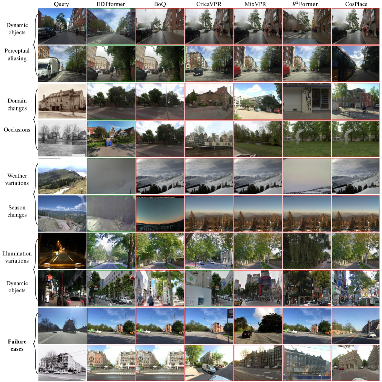
Figure 5: Qualitative results. In these challenging scenarios, our method successfully retrieves the correct images, while other methods commonly return the false places. For the first two examples, although some other methods obtain images geographically close to the query image, they exceed the set threshold (25m). For the third and fourth examples, despite image modality changes between the query and database images, our method still can retrieve the correct places by capturing the invariant and discriminative buildings. For the fifth and sixth examples, the query images are captured in natural scenes, suffering from severe condition variations and lacking discriminative landmarks. Nevertheless, our method can still match the correct place. In the seventh and eighth examples, other methods commonly return a false result due to the severe lighting changes. However, our method can produce robust and discriminative global descriptors, which can effectively handle the problem. For the last two examples, all methods fail when facing extremely difficult scenarios, in which viewpoint changes, domain variations, occlusions, dynamic objects and perceptual aliasing arise simultaneously.

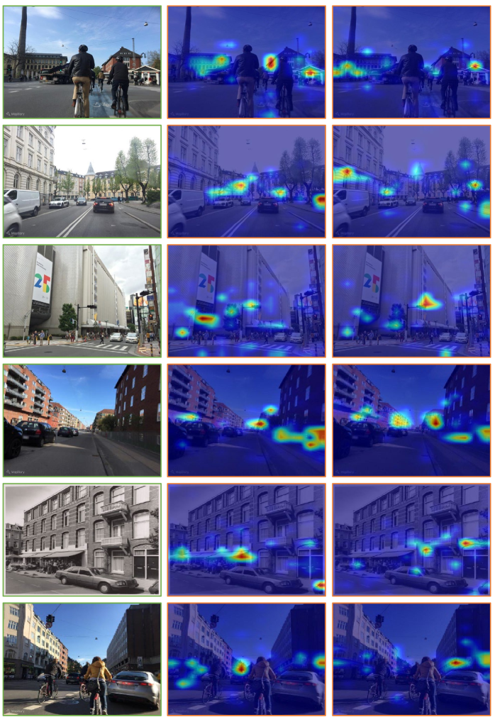
Figure 6: Visualization of learned queries. The left images with a green border show the original input images and their right counterparts with an orange border represent the attention weights of each learned query. It is worth noting that different queries prioritize different areas in the images, but they all focus on the temporarily constant and discriminative regions. On the contrary, for variable elements, these queries tend to discard them. For instance, in the first, second and last examples, all queries pay attention to the discriminative and invariant buildings and trees, while dynamic pedestrians and vehicles in the middle of the road are ignored. Thus, our method can retrieve the correct place images even if there are various changes in conditions.

Effect of the FFN in the decoder block. We simplify the transformer decoder block by removing the feedforward network (FFN) to build the EDTformer for higher efficiency. Here, we conduct a simple experiment to explain why we do that. We consistently utilize two decoder blocks to construct EDTformer with 64 learnable queries. The results presented in Table IX demonstrate that adding FFN does not enhance the overall recognition performance. Instead, it leads to an obvious performance decline on multiple benchmark datasets, such as a 4.1% R@1 decline on Nordland. We think that this is because the large number of trainable parameters introduced by the FFN hinders the model from learning and aggregating effective features. Meanwhile, it also increases the complexity of the model and introduces additional memory overhead. Therefore, using a simplified decoder can improve efficiency and get better results, which is advantageous without any drawbacks.

Ablation on the rank of LoPA. In this subsection, we further conduct ablation studies about the effect of the rank in LoPA. We consistently use the EDTformer for feature aggregation. Table X shows the results of setting different ranks. We set “w/o LoPA” as baseline. Setting the rank to 4 gets the best overall performance, but we can still achieve good results with rank even set to 2. These results show that we can achieve an outstanding performance without introducing a large number of parameters and consuming substantial memory during training. It is worth mentioning that the backbone DINOv2 is completely frozen, which indicates that the intermediate features produced by each block of DINOv2 remain consistent. The final output solely depends on how these intermediate activations are processed, which enlightens our future work to design a better parallel network to refine them. Meanwhile, due to only introducing a few parameters and memory usage, it can facilitate the application of vision foundation models under resource-limited conditions.

IV-E Qualitative experiments

Fig. 5 presents the qualitative experimental results in various challenging environments, including viewpoint variants, drastic condition changes, severe occlusions, image domain variations, etc. In the vast majority of cases, our method successfully gets similar and correct place images from the same location as the query images, while other methods tend to struggle with obtaining the correct images within the predefined threshold (25m), which demonstrates that our method is highly robust to environment changes and less prone to perceptual aliasing. For instance, in the seventh and eighth examples, the query images are captured at night. Only a small region of the image is clearly visible. However, our method still gets the correct results. Additionally, it is worth mentioning that all methods fail to obtain the correct places in the last two examples, where multiple challenges (e.g., viewpoint changes, domain variations, severe occlusions, dynamic objects and perceptual aliasing) arise simultaneously. This motivates us to further improve our method in future work to get higher accuracy and tackle more challenging scenarios.

IV-F Interpretability analysis

The experimental results presented in Table II and III have fully demonstrated the superior performance of our method. In this section, we further explore the underlying reasons. To this end, we visualize the attention weights between the input image and the learnable queries within the EDTformer. We randomly highlight two learnable queries from the outputs of the second decoder block to understand their unique learning characteristics. The results are shown in Fig. 6. Intuitively, each query has a different focus, but they all share a common characteristic. Observing horizontally, we can find that each query basically focuses on invariant yet discriminative regions (e.g., buildings and trees) while ignoring useless, dynamic and easily changing objects (e.g., sky, vehicles and pedestrians). In other words, our EDTformer successfully decodes crucial features for the VPR task into these learnable queries to achieve feature aggregation. As a result, with all information within the learnable queries combined, they can consistently concentrate on the majority of discriminative regions in the place images, which is why our method can effectively address various challenging issues in VPR.

V Conclusions

In this paper, we revisit the transformer decoder and propose a novel feature aggregation method EDTformer, a simple, efficient and powerful decoder architecture which can directly generate a robust and discriminative global representation for the place image. To be specific, EDTformer takes deep features extracted from the backbone as the keys and values, as well as a set of independent learnable queries as the queries. Then it utilizes the attention mechanism to decode and aggregate the effective features into the learnable queries, resulting in the final global representation. To further enhance the robustness, we introduce the vision foundation model DINOv2 as the backbone and design a Low-rank Parallel Adaptation method, which can adapt DINOv2 to the VPR task in a memory- and parameter-efficient way to improve the performance of the whole model. The extensive experiments show that our method effectively addresses various challenging problems in VPR and outperforms other SOTA methods on multiple benchmark datasets by a large margin.

References

- [1] G. Berton, R. Mereu, G. Trivigno, C. Masone, G. Csurka, T. Sattler, and B. Caputo, “Deep visual geo-localization benchmark,” in Proceedings of the IEEE/CVF Conference on Computer Vision and Pattern Recognition, 2022, pp. 5396–5407.
- [2] G. Bresson, Z. Alsayed, L. Yu, and S. Glaser, “Simultaneous localization and mapping: A survey of current trends in autonomous driving,” IEEE Transactions on Intelligent Vehicles, vol. 2, no. 3, pp. 194–220, 2017.
- [3] M. Xu, N. Sünderhauf, and M. Milford, “Probabilistic visual place recognition for hierarchical localization,” IEEE Robotics and Automation Letters, vol. 6, no. 2, pp. 311–318, 2020.
- [4] S. Schubert, P. Neubert, S. Garg, M. Milford, and T. Fischer, “Visual place recognition: A tutorial [tutorial],” IEEE Robotics & Automation Magazine, vol. 31, no. 3, pp. 139–153, 2024.
- [5] S. Garg, T. Fischer, and M. Milford, “Where is your place, visual place recognition?” arXiv preprint arXiv:2103.06443, 2021.
- [6] J. Li, S. Hu, Q. Li, J. Chen, V. C. M. Leung, and H. Song, “Global visual and semantic observations for outdoor robot localization,” IEEE Transactions on Network Science and Engineering, vol. 8, no. 4, pp. 2909–2921, 2021.
- [7] S. Lowry, N. Sünderhauf, P. Newman, J. J. Leonard, D. Cox, P. Corke, and M. J. Milford, “Visual place recognition: A survey,” IEEE Transactions on Robotics, vol. 32, no. 1, pp. 1–19, 2016.
- [8] H. Liu, L. Zhao, Z. Peng, W. Xie, M. Jiang, H. Zha, H. Bao, and G. Zhang, “A low-cost and scalable framework to build large-scale localization benchmark for augmented reality,” IEEE Transactions on Circuits and Systems for Video Technology, vol. 34, no. 4, pp. 2274–2288, 2024.
- [9] B. Cao, A. Araujo, and J. Sim, “Unifying deep local and global features for image search,” in European Conference on Computer Vision. Springer, 2020, pp. 726–743.
- [10] R. Wang, Y. Shen, W. Zuo, S. Zhou, and N. Zheng, “Transvpr: Transformer-based place recognition with multi-level attention aggregation,” in Proceedings of the IEEE/CVF Conference on Computer Vision and Pattern Recognition, 2022, pp. 13 648–13 657.
- [11] A. Gordo, J. Almazan, J. Revaud, and D. Larlus, “End-to-end learning of deep visual representations for image retrieval,” International Journal of Computer Vision, vol. 124, no. 2, pp. 237–254, 2017.
- [12] R. Arandjelovic, P. Gronat, A. Torii, T. Pajdla, and J. Sivic, “Netvlad: Cnn architecture for weakly supervised place recognition,” in IEEE/CVF International Conference on Computer Vision and Pattern Recognition (CVPR), 2016, pp. 5297–5307.
- [13] Y. Wang, Y. Qiu, P. Cheng, and J. Zhang, “Hybrid cnn-transformer features for visual place recognition,” IEEE Transactions on Circuits and Systems for Video Technology, vol. 33, no. 3, pp. 1109–1122, 2023.
- [14] F. Radenović, G. Tolias, and O. Chum, “Fine-tuning cnn image retrieval with no human annotation,” IEEE Transactions on Pattern Analysis and Machine Intelligence, vol. 41, no. 7, pp. 1655–1668, 2018.
- [15] Y. Ge, H. Wang, F. Zhu, R. Zhao, and H. Li, “Self-supervising fine-grained region similarities for large-scale image localization,” in European conference on computer vision. Springer, 2020, pp. 369–386.
- [16] S. Hausler, S. Garg, M. Xu, M. Milford, and T. Fischer, “Patch-netvlad: Multi-scale fusion of locally-global descriptors for place recognition,” in Proceedings of the IEEE/CVF Conference on Computer Vision and Pattern Recognition, 2021, pp. 14 141–14 152.
- [17] S. Zhu, L. Yang, C. Chen, M. Shah, X. Shen, and H. Wang, “R2former: Unified retrieval and reranking transformer for place recognition,” in Proceedings of the IEEE/CVF Conference on Computer Vision and Pattern Recognition, 2023, pp. 19 370–19 380.
- [18] Y. Xu, X. Li, H. Yuan, Y. Yang, and L. Zhang, “Multi-task learning with multi-query transformer for dense prediction,” IEEE Transactions on Circuits and Systems for Video Technology, vol. 34, no. 2, pp. 1228–1240, 2024.
- [19] X. Wang, X. Wang, B. Jiang, and B. Luo, “Few-shot learning meets transformer: Unified query-support transformers for few-shot classification,” IEEE Transactions on Circuits and Systems for Video Technology, vol. 33, no. 12, pp. 7789–7802, 2023.
- [20] M. Oquab, T. Darcet, T. Moutakanni, H. Vo, M. Szafraniec, V. Khalidov, P. Fernandez, D. Haziza, F. Massa, A. El-Nouby et al., “Dinov2: Learning robust visual features without supervision,” arXiv preprint arXiv:2304.07193, 2023.
- [21] A. Radford, J. W. Kim, C. Hallacy, A. Ramesh, G. Goh, S. Agarwal, G. Sastry, A. Askell, P. Mishkin, J. Clark et al., “Learning transferable visual models from natural language supervision,” in International conference on machine learning. PMLR, 2021, pp. 8748–8763.
- [22] L. Yuan, D. Chen, Y.-L. Chen, N. Codella, X. Dai, J. Gao, H. Hu, X. Huang, B. Li, C. Li et al., “Florence: A new foundation model for computer vision,” arXiv preprint arXiv:2111.11432, 2021.
- [23] N. Keetha, A. Mishra, J. Karhade, K. M. Jatavallabhula, S. Scherer, M. Krishna, and S. Garg, “Anyloc: Towards universal visual place recognition,” arXiv preprint arXiv:2308.00688, 2023.
- [24] F. Lu, X. Lan, L. Zhang, D. Jiang, Y. Wang, and C. Yuan, “Cricavpr: Cross-image correlation-aware representation learning for visual place recognition,” in Proceedings of the IEEE/CVF Conference on Computer Vision and Pattern Recognition (CVPR), June 2024.
- [25] F. Lu, L. Zhang, X. Lan, S. Dong, Y. Wang, and C. Yuan, “Towards seamless adaptation of pre-trained models for visual place recognition,” in The Twelfth International Conference on Learning Representations, 2024.
- [26] N. Houlsby, A. Giurgiu, S. Jastrzebski, B. Morrone, Q. De Laroussilhe, A. Gesmundo, M. Attariyan, and S. Gelly, “Parameter-efficient transfer learning for nlp,” in International Conference on Machine Learning. PMLR, 2019, pp. 2790–2799.
- [27] E. J. Hu, Y. Shen, P. Wallis, Z. AllenZhu, Y. Li, S. Wang, L. Wang, and W. Chen, “Lora: Low-rank adaptation of large language models,” arXiv preprint arXiv:2106.09685, 2021.
- [28] D. G. Lowe, “Distinctive image features from scale-invariant keypoints,” International journal of computer vision, vol. 60, no. 2, pp. 91–110, 2004.
- [29] H. Bay, A. Ess, T. Tuytelaars, and L. Van Gool, “Speeded-up robust features (surf),” Computer vision and image understanding, vol. 110, no. 3, pp. 346–359, 2008.
- [30] M. Cummins and P. Newman, “Fab-map: Probabilistic localization and mapping in the space of appearance,” The International Journal of Robotics Research, vol. 27, no. 6, pp. 647–665, 2008.
- [31] A. Angeli, D. Filliat, S. Doncieux, and J.-A. Meyer, “Fast and incremental method for loop-closure detection using bags of visual words,” IEEE transactions on robotics, vol. 24, no. 5, pp. 1027–1037, 2008.
- [32] H. Jégou, M. Douze, C. Schmid, and P. Pérez, “Aggregating local descriptors into a compact image representation,” in 2010 IEEE computer society conference on computer vision and pattern recognition. IEEE, 2010, pp. 3304–3311.
- [33] A. Ali-bey, B. Chaib-draa, and P. Giguère, “MixVPR: Feature mixing for visual place recognition,” in Proceedings of the IEEE/CVF Winter Conference on Applications of Computer Vision, 2023, pp. 2998–3007.
- [34] A. Dosovitskiy, L. Beyer, A. Kolesnikov, D. Weissenborn, X. Zhai, T. Unterthiner, M. Dehghani, M. Minderer, G. Heigold, S. Gelly et al., “An image is worth 16x16 words: Transformers for image recognition at scale,” in International Conference on Learning Representations, 2020.
- [35] A. Vaswani, N. Shazeer, N. Parmar, J. Uszkoreit, L. Jones, A. N. Gomez, Ł. Kaiser, and I. Polosukhin, “Attention is all you need,” in Advances in neural information processing systems, vol. 30, 2017.
- [36] A. Ali-bey, B. Chaib-draa, and P. Giguère, “Gsv-cities: Toward appropriate supervised visual place recognition,” Neurocomputing, vol. 513, pp. 194–203, 2022.
- [37] X. Wang, X. Han, W. Huang, D. Dong, and M. R. Scott, “Multi-similarity loss with general pair weighting for deep metric learning,” in Proceedings of the IEEE/CVF conference on computer vision and pattern recognition, 2019, pp. 5022–5030.
- [38] A. Torii, J. Sivic, T. Pajdla, and M. Okutomi, “Visual place recognition with repetitive structures,” in Proceedings of the IEEE conference on computer vision and pattern recognition, 2013, pp. 883–890.
- [39] F. Warburg, S. Hauberg, M. Lopez-Antequera, P. Gargallo, Y. Kuang, and J. Civera, “Mapillary street-level sequences: A dataset for lifelong place recognition,” in Proceedings of the IEEE/CVF conference on computer vision and pattern recognition, 2020, pp. 2626–2635.
- [40] A. Torii, R. Arandjelovic, J. Sivic, M. Okutomi, and T. Pajdla, “24/7 place recognition by view synthesis,” in Proceedings of the IEEE conference on computer vision and pattern recognition, 2015, pp. 1808–1817.
- [41] D. Olid, J. M. Fácil, and J. Civera, “Single-view place recognition under seasonal changes,” arXiv preprint arXiv:1808.06516, 2018.
- [42] B. Yildiz, S. Khademi, R. M. Siebes, and J. Van Gemert, “Amstertime: A visual place recognition benchmark dataset for severe domain shift,” in 2022 26th International Conference on Pattern Recognition (ICPR). IEEE, 2022, pp. 2749–2755.
- [43] G. M. Berton, V. Paolicelli, C. Masone, and B. Caputo, “Adaptive-attentive geolocalization from few queries: A hybrid approach,” in Proceedings of the IEEE/CVF Winter Conference on Applications of Computer Vision, 2021, pp. 2918–2927.
- [44] G. Berton, C. Masone, and B. Caputo, “Rethinking visual geo-localization for large-scale applications,” in IEEE/CVF Conference on Computer Vision and Pattern Recognition, 2022, pp. 4878–4888.
- [45] G. Berton, G. Trivigno, B. Caputo, and C. Masone, “Eigenplaces: Training viewpoint robust models for visual place recognition,” in Proceedings of the IEEE/CVF International Conference on Computer Vision, 2023, pp. 11 080–11 090.
- [46] S. Izquierdo and J. Civera, “Optimal transport aggregation for visual place recognition,” in Proceedings of the IEEE/CVF Conference on Computer Vision and Pattern Recognition (CVPR), June 2024.
- [47] F. Lu, B. Chen, X.-D. Zhou, and D. Song, “Sta-vpr: Spatio-temporal alignment for visual place recognition,” IEEE Robotics and Automation Letters, vol. 6, no. 3, pp. 4297–4304, 2021.
- [48] H. J. Kim, E. Dunn, and J.-M. Frahm, “Learned contextual feature reweighting for image geolocalization,” in Proceedings of the IEEE Conference on Computer Vision and Pattern Recognition, 2017, pp. 2136–2145.
- [49] S. Chen, C. Ge, Z. Tong, J. Wang, Y. Song, J. Wang, and P. Luo, “Adaptformer: Adapting vision transformers for scalable visual recognition,” arXiv preprint arXiv:2205.13535, 2022.
- [50] S. Jie and Z.-H. Deng, “Convolutional bypasses are better vision transformer adapters,” arXiv preprint arXiv:2207.07039, 2022.
- [51] M. B. Yi-Lin Sung, Jaemin Cho, “Lst: Ladder side-tuning for parameter and memory efficient transfer learning,” in arXiv, 2022.
- [52] O.-B. Mercea, A. Gritsenko, C. Schmid, and A. Arnab, “Time-, memory-and parameter-efficient visual adaptation,” in Proceedings of the IEEE/CVF Conference on Computer Vision and Pattern Recognition, 2024.
- [53] H. Diao, B. Wan, Y. Zhang, X. Jia, H. Lu, and L. Chen, “Unipt: Universal parallel tuning for transfer learning with efficient parameter and memory,” arXiv preprint arXiv:2308.14316, 2023.
- [54] N. Carion, F. Massa, G. Synnaeve, N. Usunier, A. Kirillov, and S. Zagoruyko, “End-to-end object detection with transformers,” in ECCV, 2020, pp. 213–229.
- [55] B. Cheng, I. Misra, A. G. Schwing, A. Kirillov, and R. Girdhar, “Masked-attention mask transformer for universal image segmentation,” arXiv, 2021.
- [56] J. Ji, R. Shi, S. Li, P. Chen, and Q. Miao, “Encoder-decoder with cascaded crfs for semantic segmentation,” IEEE Transactions on Circuits and Systems for Video Technology, vol. 31, no. 5, pp. 1926–1938, 2021.
- [57] D. Hendrycks and K. Gimpel, “Gaussian error linear units (gelus),” arXiv preprint arXiv:1606.08415, 2016.
- [58] A. Ali-bey, B. Chaib-draa, and P. Giguère, “BoQ: A place is worth a bag of learnable queries,” in Proceedings of the IEEE/CVF Conference on Computer Vision and Pattern Recognition (CVPR), June 2024, pp. 17 794–17 803.
- [59] Z. Xiong and O. Authors, “Image aesthetics assessment via learnable queries,” in ICASSP 2024-2024 IEEE International Conference on Acoustics, Speech and Signal Processing (ICASSP). IEEE, 2024, pp. 2805–2809.
- [60] M. Zaffar, S. Garg, M. Milford, J. Kooij, D. Flynn, K. McDonald-Maier, and S. Ehsan, “Vpr-bench: An open-source visual place recognition evaluation framework with quantifiable viewpoint and appearance change,” International Journal of Computer Vision (IJCV), pp. 1–39, 2021.
- [61] D. Liu, Y. Cui, L. Yan, C. Mousas, B. Yang, and Y. Chen, “Densernet: Weakly supervised visual localization using multi-scale feature aggregation,” in Proceedings of the AAAI conference on artificial intelligence, vol. 35, no. 7, 2021, pp. 6101–6109.
- [62] F. Lu, S. Dong, L. Zhang, B. Liu, X. Lan, D. Jiang, and C. Yuan, “Deep homography estimation for visual place recognition,” in Proceedings of the AAAI Conference on Artificial Intelligence, vol. 38, no. 9, 2024, pp. 10 341–10 349.
- [63] F. Perronnin, Y. Liu, J. Sánchez, and H. Poirier, “Large-scale image retrieval with compressed fisher vectors,” in 2010 IEEE Computer Society Conference on Computer Vision and Pattern Recognition. IEEE, 2010, pp. 3384–3391.
- [64] W. Bousselham, G. Thibault, L. Pagano, A. Machireddy, J. Gray, Y. H. Chang, and X. Song, “Efficient self-ensemble framework for semantic segmentation,” arXiv preprint arXiv:2111.13280, 2021.
- [65] B. Cheng, A. Schwing, and A. Kirillov, “Per-pixel classification is not all you need for semantic segmentation,” Advances in neural information processing systems, vol. 34, pp. 17 864–17 875, 2021.
- [66] B. Cheng, I. Misra, A. G. Schwing, A. Kirillov, and R. Girdhar, “Masked-attention mask transformer for universal image segmentation,” in 2022 IEEE Computer Society Conference on Computer Vision and Pattern Recognition, 2022.
- [67] M. Cuturi, “Sinkhorn distances: Lightspeed computation of optimal transport,” in Advances in Neural Information Processing Systems, vol. 26, 2013.
- [68] Z. Chen, A. Jacobson, N. Sünderhauf, B. Upcroft, L. Liu, C. Shen, I. Reid, and M. Milford, “Deep learning features at scale for visual place recognition,” in 2017 IEEE international conference on robotics and automation (ICRA). IEEE, 2017, pp. 3223–3230.