The Schrödinger equation with fractional Laplacian on hyperbolic spaces and homogeneous trees
Abstract.
We investigate dispersive and Strichartz estimates for the Schrödinger equation involving the fractional Laplacian in real hyperbolic spaces and their discrete analogues, homogeneous trees. Due to the Knapp phenomenon, the Strichartz estimates on Euclidean spaces for the fractional Laplacian exhibit loss of derivatives. A similar phenomenon appears on real hyperbolic spaces. However, such a loss disappears on homogeneous trees, due to the triviality of the estimates for small times.
Key words and phrases:
Schrödinger equation, fractional Laplacian, dispersive estimates, Strichartz estimates, real hyperbolic spaces, homogeneous trees2010 Mathematics Subject Classification:
Primary 35R11; Secondary 22E30, 35B45, 35Q41, 35R05, 43A85, 43A901. Introduction
The aim of the present work is to derive dispersive and Strichartz estimates for Schrödinger equations associated to the fractional Laplacian on negatively curved manifolds like real hyperbolic spaces and their discrete counterparts, homogeneous trees. Specifically, consider the following Cauchy problem for the fractional Schrödinger equation:
| (1) |
where stands for either (), the real hyperbolic space with its standard metric; (), the homogeneous tree with edges; or (), the Euclidean space with the flat metric. The operator represents the Fourier multiplier of order associated to powers of the corresponding Laplacian on . Here is a nonhomogeneous term defined on and , defined on , stands for the initial data.
Positive powers of the Laplace-Beltrami operator, known as the fractional Laplacian, appear in several areas of mathematical physics such as relativistic theories (see e.g., [CMB90, DL83, FLS07, LY87, LY89]).
Such operators are also reminiscent of stochastic processes with pure jumps since they are the infinitesimal generators of stable Levy processes (see the book by Bertoin [Ber96] for a detailed account). E.g. an attempt to reinterpret Feynman’s path integral into the framework of Levy processes has been undertaken in [Las02].
Additionally, significant progress has been made in understanding such operators using techniques from partial differential equations. While a comprehensive review is beyond the scope of this work, we refer readers to the books and surveys [FRRO24, Caf12, CdPF+17, Váz14] for further insights.
We now outline our main results for , namely the dispersive estimates for Equation (1). As our focus is the harmonic analysis of the multipliers on rank 1 symmetric spaces of noncompact type, we state below the boundedness properties in of the multiplier in question.
Theorem 1.1 (Dispersive estimates on hyperbolic spaces).
Consider
-
•
Assume that , , , and let
Then the following dispersive estimates hold for on
for small, say , and
for large, say .
-
•
Assume that , , and . Then the following dispersive estimates hold for on
for small, say , and
for large, say .
In Theorem 1.1, in the case , we did not state the estimates whenever since the numerology gets more tedious. We refer the reader to the dedicated Section 4.2 for more details on this case.
Note that the boundedness of such multipliers, for fixed time , was extensively investigated by Cowling, Giulini and Meda [GM90, CGM93, CGM95, CGM01, CGM02].
For specific , some results are known:
For , Equation (1) has been the subject of extensive study. Focusing specifically on symmetric spaces, key references include [AP09, IS09, APV11], while for higher-rank symmetric spaces, we refer to [AMP+23]. In addition, space-time linear estimates in the Euclidean space are the well-known Strichartz results of Ginibre-Velo [GV79, GV85] and Keel-Tao [KT98].
For , the Strichartz and dispersive estimates are due to Cho, Ozawa and Xia [COS11, CKS16]. Guo and Wang in [GW14] derived finer estimates for . This loss of derivatives is reminiscent of the Knapp phenomenon (see e.g., [GW14, Cor. 3.10.]).
For , Equation (1), often referred to as the half-wave equation, has been investigated in works such as [APV12, AP14, APV15].
In an influential paper [Gro87], Gromov investigates the so-called hyperbolic groups and provides a discrete analogue of the real hyperbolic space, namely the homogeneous trees introduced before. The next theorem provides dispersive estimates in such a setting.
Theorem 1.2 (Dispersive estimate on homogeneous trees).
Consider . Let and . Then the following dispersive estimate holds for
The previous statements follow from a fine analysis of the kernel of the propagator . A standard argument then gives Stichartz estimates from the dispersive ones. As a quick inspection shows, the phase in the oscillatory integral of the linear solution changes convexity according to the powers . This requires to consider separately the two regimes and . The kernel analysis is substantially more involved whenever is small. In particular, we observe degeneracies in this case which need to push the phase analysis an order more.
This phenomenon is dominant in the continuous setting of but disappears in the discrete one of since in this case the local analysis of the kernel becomes trivial. We point out as well to the reference [Din17] for an investigation on closed manifolds and to [Din18] for one on asymptotically Euclidean manifolds.
More generally, it has already been observed in the Euclidean case that space-time estimates exhibit a loss of derivatives (see [GW14]) which is reminiscent of the Knapp phenomenon. However, it was observed by Guo and Wang that such a loss can be removed by assuming radial symmetry. More precisely, it was also shown in [GW14] by Guo and Wang that one can obtain optimal Strichartz estimates (i.e., without loss) if one restricts to . In particular, the number is larger than and there is a gap between the Strichartz estimates for the wave operator and the ones occurring for larger powers. The loss in question occurs at small scales in space and then can be removed in the case of homogeneous trees. It is worth mentioning that the range of admissible pairs for the Strichartz estimates on is larger than the one on Euclidean spaces. This was of course already observed for . However, one still observes a loss of derivatives for general classes of data. A possible way to remove the loss would be to consider the case of data depending only on the geodesic distance to a given pole of .
The case of real hyperbolic space introduces several points departing substantially from the analysis in the Euclidean space.
-
(1)
First, we observe that the change of convexity in the phase is essential in dealing with the case of powers close to zero. This introduces a phase analysis much more technical than in the case close to .
-
(2)
Second, as already mentioned, the range of admissible exponents for the Strichartz estimates are broader than in the Euclidean case of Cho, Ozawa and Xia [COS11].
-
(3)
Interestingly enough, we notice that one can remove the loss of derivatives (the exponent in the previous theorems) provided and paying the price of a much weaker dispersion.
The loss of derivatives introduces difficulties for the well-posedness theory for the nonlinear problem. Some partial results can be found in the work by Hong and the last author [HS15], as well as several subsequent contributions by many authors. As previously mentioned, the case of radial data is more favorable and a concentration-compactness/rigidity à la Kenig-Merle, for the energy-critical nonlinear Schrödinger (NLS) is performed in [GSWZ18].
In the present article, we refrain from developing nonlinear applications of our estimates. Our original motivation is to understand the structure of the kernel of the propagator on Riemannian symmetric spaces of rank one and noncompact type. We also exclude the case in the continuous setting since it requires different techniques and is also contained in the literature (the half-wave theory, see [Tat01, APV11, MT11, MT12, AP14]).
Our paper is organized as follows: Section 2 is devoted to a summary of classical notations and preliminary tools of the harmonic analysis of symmetric spaces. Section 3 provides the refined kernel estimates, which are at the core of the proofs of the previous theorems 1.1 and 1.2. Section 4 gives the proofs of the dispersive and Strichartz estimates for the real hyperbolic spaces. Finally, Section 5 deals with the case of homogeneous trees.
Notation.
-
•
Given two non-negative functions and defined on , we write if there exists a positive constant such that for all . The expression means that and for all .
-
•
The Lebesgue spaces is denoted by , , and the time-space Strichartz spaces , , of on is defined by
In the discrete setting, we will denote the Lebesgue space by its lower-case letter .
2. Harmonic analysis tools on hyperbolic spaces
This section is devoted to some preliminary results about harmonic analysis on hyperbolic spaces together with some definitions used throughout the paper.
2.1. (Real) hyperbolic spaces
We define , for , as the upper branch of a hyperboloid in with the metric induced by the Lorenzian metric in given by . More precisely, we take
with metric where is metric on the hypersphere . Notice that via a stereographic projection, one obtains the half-space model
with the metric By choosing coordinates , , we denote the volume element by
The fact that we consider for simplicity the real case plays no role here except for simplicity of the presentation and all the formulas extend to all hyperbolic spaces, i.e., any rank one Riemannian symmetric spaces of noncompact type.
2.2. Fractional Laplacian on hyperbolic spaces
Under the parametrization of Sect. 2.1 the Laplace Beltrami operator is given by
| (2) |
Here denotes the Euclidean Laplacian in coordinates and is the partial derivative with respect to . Before defining its fractional representation, let us first recall in the Fourier transform, which is given by
Notice that the functions are generalized (in the sense that they do not belong to ) eigenfunctions of the Laplacian associated to the eigenvalue . Moreover, the following inversion formula holds
Similarly, in we consider the generalized eigenfunctions of the Laplace Beltrami operator:
where and and we denoted the Lorentzien inner product, i.e., Notice that
In analogy with the definition in , the Fourier transform can be defined as
for , . Moreover, the following inversion formula holds :
where the Plancherel density
involves the Harish-Chandra -function. It is easy to check by integration by parts for compactly supported functions, and consequently for every , that
Having in mind the theory of spherically symmetric multipliers, we define the fractional Laplacian , with , on the hyperbolic space by
Hence we can write the Schrödinger solution as
The (mild) solution to (1) on is given by
| (3) |
Our estimates and their proofs extend straightforwardly to all Riemannian symmetric spaces of noncompact type of rank (where is a noncompact semisimple connected Lie group with finite centre and is its maximal compact subgroup), i.e., to the four hyperbolic spaces: , , , , where (resp. ) denotes the field of quaternions (resp. octonions) in Table 1 and more generally to all Damek–Ricci spaces.
2.3. Asymptotic expansions of the spherical function
We now state several well-known results about asymptotic expansions of the spherical function which will be used throughout the proof of the kernel estimates in the next Section 3. To facilitate the reading, we collect those formulae into several lemmata.
We start the following integral formula due to Harish–Chandra, which holds for all (see for instance [GV88, Prop. 3.1.4], [Hel84, Ch. IV, Theorem 4.3] or [Koo84, p. 40]). We have
| (4) | ||||
where with
in the hyperboloid model of .
The following result is a large scale asymptotic (see for instance [Koo84, Formula (2.17)]).
Lemma 2.1 (Large scale asymptotic).
The following large scale converging expansion of the spherical functions holds: Let be fixed. Then for every , we have that
| (5) |
holds, where
| (6) | ||||
The coefficients in this expansion are inhomogeneous symbols of order on . More precisely, there are constants and , such that
| (7) |
Remark 2.2.
Notice that we actually have , while the other are inhomogeneous symbols of order (see for instance [APV15, Lem. 1]).
The following small scale asymptotic is due to Stanton and Tomas [ST78, Thm. 2.1].
Lemma 2.3 (Small scale asymptotics).
The following small scale expansion holds: Let be fixed. Then for every , we have
| (8) |
where
is a modified Bessel function and is the Jacobian of the exponential map, raised to the power . More precisely, for every ,
where the coefficients are smooth even functions and
Remark 2.4.
3. Kernel analysis
This section is devoted to the results in the continuous setting. The analysis relies on fine kernel estimates and we observe the dichotomy between and which amounts to investigate the two different behaviours for the phase of the oscillatory integral. The integral expression in (3) involves the following propagator
which is the radial convolution operator defined by the inverse spherical Fourier transform
| (12) |
Here is the bottom of the spectrum of on . Notice that, in comparison with the Hankel transform (i.e., the Fourier transform of radial functions in ), the modified Bessel functions are replaced in (12) by the spherical functions and the Plancherel density by , where
Remark 3.1.
Notice that for every and . Moreover, one should (often) factorize and use the fact that the parenthesis is an inhomogeneous symbol on of order .
More generally we shall consider the operator for an additional smoothness with , and its kernel
| (13) |
This will lead us to analyze oscillatory integrals
involving the phase
| (14) |
with and , and amplitudes involving and the -function.
Without loss of generality, we may assume that . The function will be the phase of the oscillatory integral associated to the propagator. As a consequence, the following technical lemmata are the basis of the kernel analysis (see Section 3.1).
Lemma 3.2 (Phase for ).
Let . Then (14) has a single stationary point , which is nonnegative and comparable to
Moreover, the following properties hold
(i) , which is positive and comparable to , is an inhomogeneous symbol of order on .
(ii) Assume that . Then, for any fixed , is comparable to when .
Proof.
Let us compute the first two derivatives
| (15) |
and
| (16) |
(i) is an immediate consequence of (16). All claims about the stationary point follow from the equation and from the behavior of the function
| (17) |
(see Figure 1), which is odd, strictly increasing and comparable to
Actually on , hence . Finally, assume that and let us estimate
where . On the one hand,
On the other hand, notice that, for ,
Hence
if , while
if . Moreover,
In conclusion, is comparable to
when . ∎
The function (17) behaves differently when . It is still odd and positive on . But now it increases between and , where it reaches its maximum , and decreases between and , where it tends to . Consequently the equation may have , or solutions.
Lemma 3.3 (Phase for ).
Let .
(i) If , (14) has no stationary point. More precisely,
| (18) |
(ii) If , (14) has a single stationary point at , where and both vanish.
(iii) If , (14) has two stationary points
Moreover, for every ,
| (19) |
(iv) If , (14) has a single stationary point at the origin. More precisely,
(v) Contrarily to and , and don’t depend on . Moreover,
is an even inhomogeneous symbol of order on ,
away from , where it vanishes, is comparable to ,
is an odd function on , which vanishes at and .
Remark 3.4.
Actually, in , we have
on , hence .
Proof of Lemma 3.3.
Almost all claims are straightforward consequences of the expressions (15), (16) and of the above behavior of (17). The only exceptions are the last point, which follows from
Hence using the lemmata above, we estimate the kernel for the dichotomy between and .
Theorem 3.5 (Kernel estimates).
(i) Assume that and . Let . Then the following estimates hold, for and
Large scale :
Small scale :
(ii) Assume that , and . Then the following estimates hold, for and
Large scale :
Small scale :
Remark 3.6.
(i) Assume that and . Then the following inequalities are equivalent
Moreover, under these conditions, we have
in the range .
(ii) Assume that and . Then the following inequalities are equivalent
Moreover, in the range , we have
Remark 3.7.
3.1. Proof of Theorem 3.5
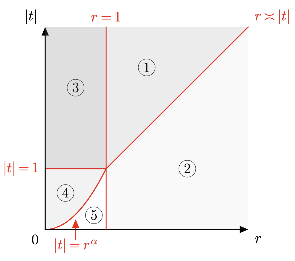
The circled numbers correspond to the different cases in the proof of Theorem 3.5. More precisely, corresponds to Subcase 1.1.1, to Subcase 1.1.2, – to Subcase 2.1.1 and to Subcase 2.1.2
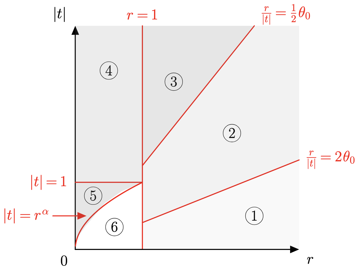
The circled numbers correspond to the different cases in the proof of Theorem 3.5 (ii). More precisely, – – correspond to Subcase 1.2, to Subcase 2.2.1, to Subcase 2.2.2 and to Subcase 2.2.3
We first explain the global structure of the proof since this is quite technical. Due to the change of behaviour in the phase in Equation (14), it is necessary to consider two regimes and . Of course, the case , which is the half-wave has been treated extensively in the literature. As explained in the introduction, the change of “convexity” of induces different losses which are a major difficulty for nonlinear applications. This also introduces several technical difficulties for the kernel analysis since for the phase has two stationary points (see Lemma 3.3) and one needs to go to the third order. Now for each of those ranges in , one needs to consider the different regimes in and , which is shown in the corresponding Figures 2 and 3. Because of similarities in the arguments, we prefer to split the proof into several parts according to:
For each of the cases above, there is additional smallness to consider in the scaled variable . We would like to emphasize that the range is the one presenting the most differences with the classical Laplacian estimates. This is because of the structure of the oscillatory integral term that such striking differences occur.
Through the proof, we will use the following version of the van der Corput Lemma (see [Ste93, Ch.VIII, Cor. p. 334]) when .
Lemma 3.8.
Let be an integer. Then there exists a constant such that
for any interval , for any function such that on , and for any function .
3.1.1. Case 1 - large spatial scale
If is bounded from below, let us say by 1, we use the large scale expansion provided by Lemma 2.1. By substituting (5) and (6) in (13), we get
where
| (22) |
with
| (23) |
Subcase 1.1. Assume that .
Subcase 1.1.1. Consider first the case where or equivalently remains bounded, let say , that is case in Figure 2. Given an even bump function such that on , let us split up
| (24) |
in (22) and
| (25) |
accordingly. On the one hand, after an integration by parts based on
| (26) |
we get
where
is a smooth function with compact support. By using Lemma 3.8 with , together with Lemma 3.2 (i) and (7), we estimate
On the other hand, after integrations by parts based on
| (27) |
we get
where
is an inhomogeneous symbol of order , according to Lemma 3.2 (ii), Lemma 3.2 (i), (23) and (7). Hence
provided that . By taking and by summing up over , we conclude that
| (28) |
when .
Subcase 1.1.2. Consider next the case where , that is case in Figure 2. Given and a bump function such that
let us now split up
and
accordingly. On the one hand, by using Lemma 3.8 with , together with Lemma 3.2 (i), (23) and (7), we estimate
On the other hand, after integrations by parts based on (27),
with
As
and
provided that . Hence
By summing up over , we conclude that
| (29) |
when and .
Subcase 1.2. Assume that . The analysis of (22) depends again on the size of .
Subcase 1.2.1. Firstly, if (see Figure 3, case ), the phase has no stationary point and, after integrations by parts based on (27), (22) becomes
where the amplitude is an inhomogeneous symbol of order , according this time to (18). Thus
provided that , and
after summing up over .
Subcase 1.2.2. Secondly, assume that (see Figure 3, case ) and let such that . Then all stationary points of the phase are contained in , according to Lemma 3.3. Let us split up (24) in (22) and (25) accordingly, where is a bump function such that on a neighborhood of and . We estimate again
by using Lemma 3.8, this time with , and
by performing integrations by parts based on (27). In conclusion,
as and are comparable under the present assumptions.
Subcase 1.2.3. Thirdly, in the remaining case (see Figure 3, case ), the phase has two stationary points : and . We shall isolate these two points by means of bump functions. Let and such that
| (30) |
where . Then and are smooth bump functions around and respectively, whose supports are disjoint and don’t contain . This follows indeed from the inequalities
Let us split up
in (22) and
| (31) |
accordingly. We estimate each term as we did in Subcase 1.1, using Lemma 3.3 instead of Lemma 3.2. This way, we obtain
| (32) |
provided that , hence
| (33) |
Remark 3.9.
All results so far, which have been proved under the assumption , hold actually for with fixed.
3.1.2. Case 2 - small spatial scale
If is bounded above, let us say by ,
we use two expressions of the spherical functions , namely Harish-Chandra integral formula (4), with and Stanton-Tomas-Ionescu formula (9) (see also Lemma 2.3).
Subcase 2.1. Assume that and , (see Figure 2, cases – – ).
Subcase 2.1.1. Consider first the range (see Figure 2, cases – ). By using (4), (13) becomes
| (34) |
where
| (35) |
We estimate (35) when by resuming the analysis in Subcase 1.1 and by dealing separately with the cases and . Let us elaborate.
If (see Figure 2, case ), the stationary point of the phase (14), with , remains bounded, according to Lemma 3.2, say for some constant . Let us split up
where
is a smooth function with compact support. By using Lemma 3.8 with , we deduce that
| (37) |
On the other hand, after integrations by parts based on
| (38) |
the second term in (36) becomes
where
is an inhomogeneous symbol of order , according to Lemma 3.2. Hence
| (39) |
provided that . By taking , we obtain finally the bound for (35) and hence
| (40) |
when .
We proceed similarly in the case (see Figure 2, case ), with the following few differences. The stationary point of the phase (14), with satisfies now , for some constant . After splitting up
in (35), the contribution of the first integral is estimated easily, while the contribution of the second integral is handled as above. Specifically, as , we have on the one hand
| (41) |
On the other hand, after integrations by parts based on (38), with , we get
| (42) |
Subcase 2.1.2. Consider next the range (see Figure 2, case ). According to Lemma 3.2, there exists such that the stationary point of the phase (14), with , satisfies . Let us split up
| (43) |
in (13) and
| (44) |
accordingly, where are even functions such that
and . Notice that the cutoff functions and have disjoint supports. By using and , we estimate easily
Let us turn to the last two terms in (44). By using the small scale asymptotics (9) with , we obtain the expressions
| (45) | ||||
and
| (46) | ||||
The main contribution arises from the first integral, which is estimated by using Lemma 3.8 with , together with Lemma 3.2 (i) and (10). This way we obtain
On the other hand, by using (11) with , we estimate
and
Finally, the third integral in (46) is estimated by performing integrations by parts based on (27), with , by using Lemma 3.2, together with (10), and by splitting up the integral
This way we obtain
As
we conclude that
Subcase 2.2. Assume that and , (see Figure 3, cases – – ).
Subcase 2.2.1 (range in Figure 3). Assume that , hence . Recall that (17) reaches its maximum at . As in Subcase 1.2, let such that . We may assume that by reducing the range , according to Remark 3.9. Let us estimate by considering again several cases.
Assume first that . According to Lemma 3.3 (iv), the phase (14), with , has a single stationary point at the origin. Given an even bump function such that
where , let us split up the integral as in (24) and the kernel
| (47) |
accordingly. On the one hand, after an integration by parts based on (26), we obtain
and deduce that
by applying Lemma 3.8 with . On the other hand, after performing integrations by parts based on (26), we obtain
which is if . As a first conclusion, we obtain
when and .
Assume next that . According to Lemma 3.3 (iii), the phase (14), with , has two stationary points : , which is comparable to , and , which is comparable to . Given another even bump function such that
where , let us split up
in (13) and
| (48) |
accordingly. As far as the first term in (48) is concerned, we obtain
either by using the phase (14) with as above, or by using (4) and the phase (14) with as in the proof of (37). We claim that the second term in (48) is , for every integer . This is achieved by substituting (4) in
and by performing integrations by parts based on (38) with , after observing that the stationary points of the phase (14), with , remain outside . Let us turn to the third term in (48), which reads
after substituting (9). We estimate the main term
by using Lemma 3.8 with , together with Lemma 3.3 (iii) and (10), and the remainder
by using (11). Consider finally the last term in (48), which reads similarly
We estimate
by performing integrations by parts based on (27) and by using Lemma 3.3 (iii) and (v), together with (10), and
by using (11). In conclusion,
when and .
Remark 3.10.
We obtain in particular when .
Subcase 2.2.2 (range in Figure 3). Assume that and satisfy , hence . We argue as in Subcase 2.2.1 with a few differences. By reducing , we may assume again that .
When , we split again as in (47). On the one hand, we estimate trivially
On the other hand, we estimate
by splitting up
More precisely, the contribution of the first integral is trivially bounded by
while the contribution of the second integral is bounded, after integrations by parts based on (26), by
As first conclusion, we obtain when and .
When , we split again as in (44). This time, we estimate
trivially and both , by
as in Subcase 2.2.1. Finally, we split up
according to
On the one hand, we estimate
by using , and
by substituting (4), by performing integrations by parts based on (38) and by using (19).
In conclusion,
when .
Remark 3.11.
We obtain in particular when .
Subcase 2.2.3 (range in Figure 3). Assume that . Notice that
According to Lemma 3.3, there exists such that all critical of the phase (14), with , are contained in . Given a smooth even bump function on such that on and , let us split up
and
accordingly. On the one hand, we estimate
by using . On the other hand, we estimate
by substituting (4), by performing integrations by parts based on (38) and by using (19).
In conclusion,
when .
Remark 3.12.
We obtain again when .
4. Dispersive and Strichartz estimates on hyperbolic spaces
We now deduce from Theorem 3.5 dispersive and Strichartz estimates, following the standard strategy of Ginibre and Velo, combined with the Kunze–Stein phenomenon, as in [AP09, IS09, APV11, APV12, AP14, APV15]. More precisely, we will use the following version of the Kunze–Stein phenomenon (see [APV11, Thm. 4.2]).
Lemma 4.1.
Let . Then there exists a positive constant such that, for every and for every measurable radial function on ,
Remark 4.2.
Notice that
| (49) |
The proof of the Strichartz estimates uses the standard argument, Young’s inequality extended to weak type spaces (see for instance [Gra14, Thm. 1.4.25]), the Christ-Kiselev Lemma [CK01] for the non-endpoint estimates and the Bourgain or Keel-Tao trick [KT98] for the endpoint estimates, as in [APV11, Sect. 6] or [AP14, Sect. 5] for instance. Therefore we generally omit proofs of the Strichartz estimates in this paper.
4.1. Case
Theorem 4.3 (Dispersive estimates).
Let , , and set
| (50) |
Then the following dispersive estimates hold for
for small, say , and
for large, say .
Remark 4.4.
These estimates become in particular
when .
Proof.
All estimates rely on the kernel estimates in Theorem 3.5 (i) extended straightforwardly to the vertical strip in . More precisely, the estimates for small are obtained by interpolation for an analytic family of operators (see for instance [SW71, Ch. V, Thm. 4.1] or [Gra14, Thm. 1.3.7]) between
| (51) |
and
While the estimate for large follows from
and from Lemma 4.1. ∎
Theorem 4.5 (Strichartz inequalities).
Remark 4.6.
As already observed for the Schrödinger equation and for the wave equation , the admissible region is much larger on hyperbolic spaces than on Euclidean spaces.
4.2. Case
From the kernel estimates in Theorem 3.5 (ii), we deduce similarly the following inequalities.
Theorem 4.7 (Dispersive estimates).
(i) Assume that , , and . Then the following dispersive estimates hold
| (52) |
for small, say , and
| (53) |
for large, say .
(ii) In dimension , the small time estimate is the same, while the large time estimate reads
The estimate (53) is fine for large but, as tends to , the smoothness factor doesn’t vanish, as might be expected. Let us therefore refine (53) as follows.
Corollary 4.8.
Assume that , , and let . Then the following dispersive estimate holds for large, say
| (54) |
Proof.
Theorem 4.9 (Strichartz inequalities).
Remark 4.10.
In this statement, the interval must be actually reduced to the smaller interval , where
When and , we have indeed and the admissibility condition boils down to the trivial endpoint , .
Proof.
Referring to the proofs of [APV11, Thm. 6.3] and [AP14, Thm. 5.2], we shall be content to explain and comment the admissibility conditions
| (56) |
occurring in (55). Recall that the above-mentioned proofs consist mainly in estimating
| (57) |
and
| (58) |
On the one hand, we deduce (57) from the dispersive estimate (52), which yields
and from Young’s inequality (see for instance [Gra14, Thm. 1.4.25]) provided that is and . This way we obtain (57) under the assumptions
and except for the endpoint
| (59) |
The first case is handled by the refined analysis in [KT98] while the second one is excluded.
On the other hand, we prove (58) under the assumptions
by considering separately the ranges , and , where
Remark 4.11.
In dimension , Theorem 4.9 holds for the following admissible region
For fixed , the admissible set of couples looks like Figure 5, with
and, in the limit case , this set boils down to the diagonal
As a general observation, we would like to emphasize that the admissible range of exponents when the power of the Laplacian is below one, i.e., close to a very small diffusion, is smaller than the one for powers closer to the standard diffusion . This is due to a combination of two effects: one is due to the necessary loss of derivatives which cannot be made arbitrarily small but also the behaviour of the kernel in this low diffusive case which is more similar to an Euclidean one. On the other hand, in the regime of higher diffusion, one observes a behaviour much more influenced by the negative curvature. From the point of view of nonlinear applications, this introduces substantial difficulties to prove well-posedness.
5. Homogeneous trees
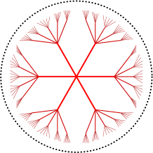
In this section, we consider the discrete analogs of hyperbolic spaces which are homogeneous trees and more precisely hyperbolic space according to Gromov [Gro87]. Specifically, for , a homogeneous tree of degree is an infinite connected graph with no loops, in which every vertex is adjoint to other vertices (see Figure 7). We denote by the set of vertices in the homogeneous tree with edges, equipped with the counting measure.
Recall that the combinatorial Laplacian on is defined by
and that its spectrum is equal to
,
where .
Here is the number of edges of the shortest path joining and . We refer to [Car73, FTN91, CMS98] for some basic tools of harmonic analysis on .
Among earlier works about (1) on homogeneous trees, let us mention
-
•
[Set98], which is devoted to the heat equation with continuous time associated with the Laplacian on ,
-
•
[Stó11], which is devoted to the heat equation with continuous time associated with the fractional Laplacian on ,
-
•
[MS99], which is devoted to the wave equation with continuous time associated with the shifted Laplacian on ,
-
•
[Edd13a], which is devoted to the Schrödinger equation with continuous time associated with the Laplacian on .
The equation (1) on is solved and analyzed as the corresponding equation on . The main differences lie in the local (in time) analysis, which is trivial, and in the spectrum, which is compact. More precisely, we have again Duhamel’s formula (3) where
is the convolution operator defined by the radial kernel
| (60) |
Here , , and
| (61) |
is the spherical function of index . By substituting (61) in (60), we obtain
| (62) |
where .
Lemma 5.1 (Stationary phase analysis).
Let and assume that .
(i) The phase function has two stationary points on the circle
Moreover, and .
(ii) There exists such that the phase function has
(iii) Moreover, we have the following additional information about the last case. For every , there exist open subsets in and a constant such that, whenever ,
,
outside and on .
Proof.
Let us compute the first derivatives
| (63) |
Consider the expression
which occurs in (63) and which is a –periodic even function on , with
On , the function may increase before decreasing, as its derivatives
vanishes at , at and at most once on . In particular, and hence
-
•
vanishes at a single point in , which belongs to ,
-
•
is strictly positive on ,
-
•
is strictly negative on .
Thus , which is a –periodic odd function on , increases (strictly) on , from to , and decreases back on , from to . Consequently,
for every , the equation has exactly two solutions in :
and .
Let and assume that . Then the phase function has two stationary points in , namely and . Moreover,
-
•
are neighborhoods of in such that on and ,
-
•
are neighborhoods of in such that on and .
∎
Remark 5.2.
In the limit case , we have
, ,
hence
, , , .
Theorem 5.3 (Kernel estimate).
Assume that . Then the following kernel estimate holds
| (64) |
Moreover, there exists such that
| (65) |
if .
Remark 5.4.
Proof of Theorem 5.3.
Without loss of generality, we may assume that . The estimate (64) follows immediately from the expression (62), where the integrand is bounded. Let us improve (64) when and is small, so that Lemma 5.1 (iii) applies. First, we perform an integration by parts based on
This way, (62) becomes
| (66) |
where is bounded, as well as its derivatives. Next, we estimate (66) by stationary phase analysis based on Lemma 5.1 (iii). Specifically, given a smooth function on such that on and , we split up the integral in (66) as follows :
On the one hand, the main estimate
is obtained by applying Lemma 3.8 with . On the other hand, the remainder estimate
is obtained after integrations by parts based on
This concludes the proof of (65). ∎
Let us turn to mapping properties of the Schrödinger operator . As in [Edd13a, Thm. 3.4 and Cor. 3.5], let us deduce the following result from Theorem 5.3.
Corollary 5.5 (Dispersive estimate).
Let and . Then the following dispersive estimate holds for
Similar, we can conclude from Theorem 5.3 and [Edd13a, Thm. 3.6] the following result for the inhomogeneous case.
Corollary 5.6 (Strichartz estimates).
Let and with . Then the following Strichartz estimates hold for solutions of (1) on
Here and belong to the square see Figure 8
and depends on , , but not on and .
Remark 5.7.
Notice that, in the discrete setting and contrary to the continuous setting, the case half-wave equation is similar to the general case .
Let us mention that for the nonlinear Schrödinger (NLS) equation on homogenous trees
| (67) |
where
for some exponent , we get similar local and global well-posedness results as in [Edd13a, Thm. 4.1.] for .
Theorem 5.8.
Let Then the nonlinear Schrödinger equation (67) is
-
•
locally well-posed for arbitrary initial data in ,
-
•
globally well-posed for small initial data in ,
-
•
globally well-posed for arbitrary initial data in under the additional gauge invariant condition .
Acknowledgments
G. Palmirotta receives funding from the German Research Foundation via the grant SFB-TRR 358/1 2023 — 491392403. Y. Sire is partially supported by NSF DMS Grant , "Regularity vs singularity formation in elliptic and parabolic equations".
References
- [AMP+23] J.-Ph. Anker, S. Meda, V. Pierfelice, M. Vallarino, and H.-W. Zhang, Schrödinger equation on non-compact symmetric spaces, J. Differ. Equ. 356 (2023), 163–187.
- [AP09] J.-Ph. Anker and V. Pierfelice, Nonlinear Schrödinger equation on real hyperbolic spaces, Ann. Inst. Henri Poincaré (C), Analyse Non Linéaire 26 (2009), no. 5, 1853–1869.
- [AP14] by same author, Wave and Klein-Gordon equations on hyperbolic spaces, Anal. PDE 12 (2014), no. 4, 953–995.
- [APV11] J.-Ph. Anker, V. Pierfelice, and M. Vallarino, Schrödinger equations on Damek-Ricci spaces, Comm. Part. Differ. Equ. 36 (2011), no. 6, 976–997.
- [APV12] by same author, The wave equation on hyperbolic spaces, J. Differ. Equ. 252 (2012), no. 10, 5613–5661.
- [APV15] by same author, The wave equation on Damek-Ricci spaces, Ann. Mat. Pura Appl. 194 (2015), no. 3, 731–758.
- [Ber96] J. Bertoin, Lévy processes, Cambridge Tracts Math., vol. 121, Cambridge Univ. Press, 1996.
- [Caf12] L. Caffarelli, Non-local diffusions, drifts and games, Nonlinear partial differential equations, Abel Symp., vol. 7, Springer, Heidelberg, 2012, pp. 37–52.
- [Car73] P. Cartier, Géométrie et analyse sur les arbres, Séminaire Bourbaki vol. 1971/72 Exposés 400–417, Springer, 1973, pp. 123–140.
- [CdPF+17] A. Carrillo, J., M. del Pino, A. Figalli, G. Mingione, and J. L. Vázquez, Nonlocal and nonlinear diffusions and interactions new methods and directions, Lect. Notes Math., vol. 2186, Springer, Cham;, 2017, CIME Course, Cetraro, July 4–8, 2016, M. Bonforte and G. Grillo (eds.).
- [CGM93] M. Cowling, S. Giulini, and S. Meda, estimates for functions of the Laplace-Beltrami operator on noncompact symmetric spaces. I, Duke Math. J. 72 (1993), no. 1, 109–150.
- [CGM95] by same author, estimates for functions of the Laplace-Beltrami operator on noncompact symmetric spaces. II, J. Lie Theory 5 (1995), 1–14.
- [CGM01] by same author, estimates for functions of the Laplace-Beltrami operator on noncompact symmetric spaces. III, Ann. Inst. Fourier 51 (2001), no. 4, 1047–1069.
- [CGM02] by same author, Oscillatory multipliers related to the wave equation on noncompact symmetric spaces, J. London Math. Soc. (2) 66 (2002), no. 3, 691–709.
- [CK01] M. Christ and A. Kiselev, Maximal functions associated to filtrations, J. Funct. Anal. 179 (2001), no. 2, 409–425.
- [CKS16] C.-H. Cho, Y. Koh, and I. Seo, On inhomogeneous Strichartz estimates for fractional Schrödinger equations and their applications, Discrete Contin. Dyn. Syst. 36 (2016), no. 4, 1905–1926.
- [CMB90] R. Carmona, W. Masters, and Simon B., Relativistic Schrödinger operators: Asymptotic behavior of the eigenfunctions, J. Funct. Anal. 91 (1990), no. 1, 11–142.
- [CMS98] M. Cowling, S. Meda, and A. Setti, An overview of harmonic analysis on the group of isometries of a homogeneous tree, Expo. Math. 16 (1998), no. 5, 385–423.
- [COS11] Y. Cho, T. Ozawa, and Xia S., Remarks on some dispersive estimates, Comm. Pure Appl. Anal. 10 (2011), no. 4, 1121–1128.
- [Din17] V. D. Dinh, Strichartz estimates for the fractional Schrödinger and wave equations on compact manifolds without boundary, J. Differ. Equ. 263 (2017), no. 12, 8804–8837.
- [Din18] by same author, Global in time Strichartz estimates for the fractional Schrödinger equations on asymptotically Euclidean manifolds, J. Funct. Anal. 275 (2018), no. 8, 1943–2014.
- [DL83] I. Daubechies and E.H. Lieb, One-electron relativistic molecules with Coulomb interaction, Comm. Math. Phys. 90 (1983), no. 4, 497–510.
- [DLM] Digital Library of Mathematical Functions, National Institute of Standards and Technology.
- [Edd13a] A. Jamal Eddine, Schrödinger equation on homogeneous trees, J. Lie Theory 23 (2013), 779–794.
- [Edd13b] by same author, Schrödinger equation on homogeneous trees, arXiv:1206.0835v2 (2013).
- [FLS07] R.L. Frank, E.H. Lieb, and R. Seiringer, Stability of relativistic matter with magnetic fields for nuclear charges up to the critical value, Comm. Math. Phys. 275 (2007), no. 2, 479–489.
- [FRRO24] X. Fernández-Real and X. Ros-Oton, Integro-differential elliptic equations, Progress in Mathematics, vol. 350, Birkhäuser/Springer, Cham, 2024.
- [FTN91] A. Figà-Talamanca and C. Nebbia, Harmonic analysis and representation theory for groups acting on homogeneous trees, vol. 162, Cambridge University Press, 1991.
- [GM90] S. Giulini and S. Meda, Oscillating multipliers on noncompact symmetric spaces, J. Reine Angew. Math. 409 (1990), 93–105.
- [Gra14] L. Grafakos, Classical Fourier analysis (3rd edition), Graduate Texts in Mathematics, vol. 249, Springer, 2014.
- [Gro87] M. Gromov, Hyperbolic groups, Essays in group theory, Springer, 1987, pp. 75–263.
- [GSWZ18] Z. Guo, Y. Sire, Y. Wang, and L. Zhao, On the energy-critical fractional Schrödinger equation in the radial case, Dyn. Partial Differ. Equ. 15 (2018), no. 4, 265–282.
- [GV79] J. Ginibre and G. Velo, On a class of nonlinear Schrödinger equations. I. The Cauchy problem, general case, J. Funct. Anal. 32 (1979), no. 1, 1–32.
- [GV85] by same author, The global Cauchy problem for the non linear Schrödinger equation revisited, Ann. Institut Henri Poincaré C, Analyse non linéaire 2 (1985), no. 4, 309–327.
- [GV88] R. Gangolli and V.S. Varadarajan, Harmonic analysis of spherical functions on real reductive groups, Erg. Math. Grenzgeb. Folge 2, vol. 101, Springer–Verlag, 1988.
- [GW14] Z. Guo and Y. Wang, Improved Strichartz estimates for a class of dispersive equations in the radial case and their applications to nonlinear Schrödinger and wave equations, J. Anal. Math. 124 (2014), 1–38.
- [Hel84] S. Helgason, Groups and geometric analysis. Integral geometry, invariant differential operators, and spherical functions, Academic Press (1984), Amer. Math. Soc. (2000), 1984.
- [HS15] Y. Hong and Y. Sire, On fractional Schrödinger equations in Sobolev spaces, Commun. Pure Appl. Anal. 14 (2015), no. 6, 2265–2282.
- [Ion00] A.D. Ionescu, Fourier integral operators on noncompact symmetric spaces of real rank one, J. Funct. Anal. 174 (2000), no. 2, 274–300.
- [IS09] A.D. Ionescu and G. Staffilani, Semilinear Schrödinger flows on hyperbolic spaces: Scattering in , Math. Ann. 345 (2009), 133–158.
- [Koo84] T.H. Koornwinder, Jacobi functions and analysis on noncompact semisimple lie groups, in Special functions: Group theoretical aspects and applications, R.A. Askey and al. (eds.), Reidel (1984), 1–85.
- [KT98] M. Keel and T. Tao, Endpoint Strichartz estimates, Amer. J. Math. 120 (1998), no. 5, 955–980.
- [Las02] N. Laskin, Fractional Schrödinger equation, Phys. Rev. E (3) 66 (2002), no. 5, 7.
- [LY87] E.H. Lieb and H.-T. Yau, The Chandrasekhar theory of stellar collapse as the limit of quantum mechanics, Comm. Math. Phys. 112 (1987), no. 1, 147–174.
- [LY89] by same author, The stability and instability of relativistic matter, Comm. Math. Phys. 118 (1989), no. 2, 177–213.
- [MS99] G. Medolla and A.G. Setti, The wave equation on homogeneous trees, Ann. Mat. Pura Appl. 176 (1999), no. 4, 1–27.
- [MT11] J. Metcalfe and M.E. Taylor, Nonlinear waves on 3D hyperbolic space, Trans. Amer. Math. Soc. 363 (2011), no. 7, 3489–3529.
- [MT12] by same author, Dispersive wave estimates on 3D hyperbolic space, Proc. Amer. Math. Soc. 140 (2012), no. 11, 3861–3866.
- [Set98] A.G. Setti, and operator norm estimates for the complex time heat operator on homogeneous trees, Trans. Amer. Math. Soc. 350 (1998), no. 2, 743–768.
- [ST78] R.J. Stanton and P.A. Tomas, Expansions for spherical functions on noncompact symmetric spaces, Acta Math. 140 (1978), 251–276.
- [Ste93] E.M. Stein, Harmonic analysis. Real–variable methods, orthogonality and oscillatory integrals, Princeton Math. Series, vol. 43, Princeton Univ. Press, 1993.
- [Stó11] A. Stós, Stable semigroups on homogeneous trees and hyperbolic spaces, Illinois J. Math. 55 (2011), no. 4, 1437–1454.
- [SW71] E.M. Stein and G. Weiss, Introduction to Fourier Analysis on Euclidean Spaces, Princeton Math. Series, vol. 32, Princeton Univ. Press, 1971.
- [Tat01] D. Tataru, Strichartz estimates in the hyperbolic space and global existence for the semilinear wave equation, Trans. Amer. Math. Soc. 353 (2001), no. 2, 795–807.
- [Váz14] J.L. Vázquez, Recent progress in the theory of nonlinear diffusion with fractional Laplacian operators, Discrete Contin. Dyn. Syst. Ser. 7 (2014), no. 4, 857–885.