Counter-monotonic Risk Sharing with
Heterogeneous Distortion Risk Measures

Abstract

We study risk sharing among agents with preferences modeled by heterogeneous distortion risk measures, who are not necessarily risk averse. Pareto optimality for agents using risk measures is often studied through the lens of inf-convolutions, because allocations that attain the inf-convolution are Pareto optimal, and the converse holds true under translation invariance. Our main focus is on groups of agents who exhibit varying levels of risk seeking. Under mild assumptions, we derive explicit solutions for the unconstrained inf-convolution and the counter-monotonic inf-convolution, which can be represented by a generalization of distortion risk measures. Furthermore, for a group of agents with different levels of risk aversion or risk seeking, we consider a portfolio manager’s problem and explicitly determine the optimal investment strategies. Interestingly, we observe a counterintuitive phenomenon of comparative statics: even if all agents in the group become more risk seeking, the portfolio manager acting on behalf of the group may not necessarily allocate a larger proportion of investments to risky assets, which is in sharp contrast to the case of risk-averse agents.

1 Introduction

Risk-exchange markets, such as insurance, reinsurance, or financial markets, are central to modern economics. The primary focus of studying such markets has traditionally been the determination of an optimal, or efficient redistribution of the aggregate market risk, through contracts or trading mechanisms, among market participants, henceforth referred to as agents. The seminal work of Borch, (1962) and Wilson, (1968) showed that within the framework of Expected-Utility Theory (EUT), Pareto-optimal allocations between risk-averse agents are comonotonic, and they can therefore be expressed as nondecreasing functions of the aggregate market risk. This is a cornerstone result in the theory of risk sharing, and it is often seen as a foundational justification for risk pooling, since each agent’s risk allocation at an optimum depends only the realization of the aggregate risk. Numerous extensions beyond EUT have been studied in the literature, with the perennial assumption of (strong) risk aversion, that is, monotonicity with respect to the concave order. The literature is vast, and we refer for instance to the work of Chateauneuf et al., (2000), Dana, (2002, 2004), Tsanakas and Christofides, (2006), De Castro and Chateauneuf, (2011), Beißner and Werner, (2023), and Ravanelli and Svindland, (2014) for several models of ambiguity-sensitive preferences.

A milestone result in this direction is the so-called comonotonic improvement theorem (e.g., Landsberger and Meilijson, (1994), Dana, (2004), Ludkovski and Rüschendorf, (2008), Carlier et al., (2012), or Denuit et al., (2025)), an important implication of which is that risk-averse agents always prefer comonotone allocations, and that Pareto optima are comonotonic under strict risk aversion. This naturally led Boonen et al., (2021) to examine the so-called comonotone market, an incomplete market in which only comonotonic allocations are feasible. Pareto-optimal risk sharing in comonotone markets was also studied by Liu, (2020) and Ghossoub and Zhu, (2024).

In the risk measurement literature, Pareto-optimal risk sharing between agents with convex or coherent risk measures has been widely studied as well. We refer to Barrieu and El Karoui, (2005), Acciaio, (2007), Jouini et al., (2008), Filipović and Svindland, (2008), Mastrogiacomo and Rosazza Gianin, (2015), and the references therein, for instance. Additionally, Pareto-optimal risk sharing between agents with quantile-based risk measures that are not necessarily convex was examined by Embrechts et al., (2018, 2020), Liu, (2020), Liebrich, (2024) and Ghossoub et al., 2024b , for instance.

The characterization of optimal allocations in risk sharing markets involving agents who are not risk-averse remains relatively underexplored. Recent studies on quantile-based risk sharing, including Embrechts et al., (2018, 2020) and Weber, (2018), identified a pairwise counter-monotonic structure — the opposite of comonotonicity — in the optimal allocations. Furthermore, Lauzier et al., 2023b provided explicit Pareto-optimal allocations among agents using the inter-quantile difference, demonstrating that the optimal allocation exhibits a mixture of pairwise counter-monotonic structures.. As a dependence concept, pairwise counter-monotonicity has been studied by Dall’Aglio, (1972), Dhaene and Denuit, (1999) and Cheung and Lo, (2014). Parallel to the comonotone improvement theorem, Lauzier et al., (2024) established the so-called counter-monotonic improvement theorem, leading to an implication that counter-monotonic allocations will always be preferred by risk-seeking agents. Based on the counter-monotonic improvement theorem, Ghossoub et al., 2024a provided a systematic study of risk sharing in markets where only counter-monotonic allocations are allowed, and they gave an explicit characterization of the optimal allocations when agents are risk-averse and risk-seeking. Their analysis assumes that the preferences of the agents are modelled by a common distortion risk measure.

This paper extends the previous work by examining a market where agents may have heterogeneous risk preferences, and they are not necessarily risk averse. It is notable that although agents within a group may differ in their levels of risk aversion, we assume that all agents in the same group are either all risk-averse or all risk-seeking. We do not consider cases where both risk-averse and risk-seeking agents are combined in a single group. The key novel insights and extensions are summarized as follows:

• In the homogeneous case, Ghossoub et al., 2024a established a universal ordering among the three versions of inf-convolution: unconstrained, counter-monotonic, and comonotonic, from the smallest to the largest. In contrast to the homogeneous case, the ordering between the comonotonic and counter-monotonic versions of the inf-convolution depends on the distortion functions.

• When agents have identical concave distortion functions (the case of risk aversion), the three versions of inf-convolution have identical values, as shown in Theorem 3 of Ghossoub et al., 2024a . However, for a group of risk-averse agents with different levels of risk aversion, counter-monotonic allocations are generally not Pareto optimal, leading to a gap between the three versions of inf-convolution.

• Under some mild conditions, we derive an explicit formula for the counter-monotonic inf-convolution in the case where agents are risk seeking, characterized by different convex distortion functions.

• We consider a portfolio manager’s problem, where the portfolio manager needs to determine how much to invest in risky assets and how to allocate the payoffs to participants. In the homogeneous case, when the agents in one group become more risk-seeking, the group as a whole exhibits more risk-seeking behavior; specifically, a manager investing on behalf of this group would tend to invest more in risky assets. In contrast, in the heterogeneous case, even if each agent individually becomes more risk-seeking, the group as a whole may not necessarily exhibit a correspondingly more risk-seeking behavior.

The rest of the paper is organized as follows. Sections 2 and 3 contain preliminaries on risk measures and on risk sharing problems, respectively. In particular, Section 3 recalls the counter-monotonic improvement theorem (reported as Theorem 1) and some related discussions on counter-monotonicity. In Section 4, we analyze the counter-monotonic risk sharing problem and obtain general relations for different choices of the distortion functions (Theorem 2). We specialize to risk-seeking agents in Section 5. Based on the counter-monotonic improvement theorem, counter-monotonic inf-convolutions are determined explicitly for risk-seeking agents (Theorem 3). Applying these results, we solve the portfolio optimization problem, as detailed in Section 6. Section 7 concludes the paper.

2 Preliminaries

2.1 Risk measures and basic terminology

Let $(\Omega,\mathcal{F},\mathbb{P})$ be an atomless probability space and $\mathcal{X}$ a convex cone of random variables on this space. Section 4 considers $\mathcal{X}=L^{\infty}$, the set of all essentially bounded random variables, and Sections 5 and 6 consider $\mathcal{X}=L^{+}$ or $\mathcal{X}=L^{-}$, where $L^{+}$ (resp. $L^{-}$) represents the sets of nonnegative (resp. nonpositive) essentially bounded random variables. Almost surely equal random variables are treated as identical. Throughout, the random variable $X\in\mathcal{X}$ represents losses, and its negative values represent gains. We denote by $\mathbb{1}_{A}$ the indicator function for an event $A\in\mathcal{F}$. Let

$$\mathcal{H}^{\rm BV}=\{h:[0,1]\to\mathbb{R}\mid h\text{ is of bounded variation and }h(0)=0\}.$$

Next, we present the definition of a distortion riskmetric.

Definition 1.

A distortion riskmetric is a mapping $\rho_{h}:\mathcal{X}\to\mathbb{R}$ given by

$$\rho_{h}(X)=\int X\mathrm{d}\left(h\circ\mathbb{P}\right)=\int_{0}^{\infty}h(\mathbb{P}(X\geqslant x))\,\mathrm{d}x+\int_{-\infty}^{0}(h(\mathbb{P}(X\geqslant x))-h(1))\,\mathrm{d}x,$$

for some $h\in\mathcal{H}^{\rm BV}$.

We note that the elements of $\mathcal{H}^{\rm BV}$ are not necessarily monotone. If we constrain $h\in\mathcal{H}^{\rm BV}$ to be increasing and normalized, that is, $h\in\mathcal{H}$, where

$$\mathcal{H}=\{h:[0,1]\to[0,1]\mid h\,\text{is increasing and }h(0)=1-h(1)=0\},$$

then the distortion riskmetric $\rho_{h}$ for $h\in\mathcal{H}$ is a distortion risk measure. Here and throughout, terms like “increasing” or “decreasing” are in the non-strict sense. In this paper, the agents’ risk preferences are modeled by the class of distortion risk measures. The more general class of distortion riskmetrics is introduced since it will be useful in our further analysis. In particular, we show in the setting of Section 5 that the comonotonic inf-convolution of distortion risk measures is a distortion risk measure, whereas their counter-monotonic inf-convolution is a distortion riskmetric.

The dual $\tilde{h}$ of a given $h\in\mathcal{H}^{\rm BV}$, which will be useful in many of our results, is defined as

$$\tilde{h}(t)=h(1)-h(1-t),\ \mbox{~~~~for all $t\in[0,1]$,}$$

and it is an element of $\mathcal{H}^{\rm BV}$. If $h$ is in $\mathcal{H}$, then so is $\tilde{h}$. The dual of $\tilde{h}$ is equal to $h$, and the two corresponding distortion riskmetrics are connected via the equality

$$\rho_{h}(X)=-\rho_{\tilde{h}}(-X),\mbox{~~~~for all $X\in\mathcal{X}$.}$$

We now recall some properties of distortion riskmetrics that we use throughout. A distortion riskmetric $\rho_{h}$ may have the following properties as a functional $\rho:\mathcal{X}\mapsto\mathbb{R}$.

1. Law-invariance: $\rho(X)=\rho(Y)$ if $X$ and $Y$ have the same distribution, i.e., $X\stackrel{{\scriptstyle\mathrm{d}}}{{=}}Y$;

2. Positive homogeneity: $\rho(\lambda X)=\lambda\rho(X)$ for any $\lambda>0$;

3. Translation invariance: $\rho(X+c)=\rho(X)+c$ for $c\in\mathbb{R}$ and $X+c\in\mathcal{X}$;

4. Comonotonic additivity: $\rho(X+Y)=\rho(X)+\rho(Y)$ if $X$ and $Y$ are comonotonic;

5. Subadditivity: $\rho(X+Y)\leqslant\rho(X)+\rho(Y)$;

6. Convex order consistency: $\rho(X)\leqslant\rho(Y)$ if $X\leqslant_{\rm cx}Y$, where the inequality is the convex order, meaning $\mathbb{E}[u(X)]\leqslant\mathbb{E}[u(Y)]$ for all convex functions $u$ such that the two expectations are well-defined;

7. Monotonicity: $\rho(X)\leqslant\rho(Y)$ if $X\leqslant Y$.

In fact, these properties do not always hold for a distortion riskmetric $\rho_{h}$. To be more specific, all distortion riskmetric $\rho_{h}$ satisfy (a), (b), and (d). Property (c) holds true if $h(1)=1$. By Wang et al., 2020b (, Theorem 3), conditions (e) and (f) are equivalent to the concavity of $h$. Condition (g) is equivalent to increasing monotonicity of $h$. The four properties (b), (c), (e) and (g) together defines a coherent risk measure in the sense of Artzner et al., (1999), corresponding to an increasing and concave $h$ with $h(1)=1$ for $\rho_{h}$. For various characterizations and properties of distortion riskmetrics, see Wang et al., 2020b on $L^{\infty}$ and Wang et al., 2020a on more general spaces. Convex order in (f) and its related notions are popular for modeling risk aversion in decision theory (Rothschild and Stiglitz,, 1970), and it is also widely studied actuarial science and risk management (Rüschendorf,, 2013; He et al.,, 2016).

Many popular risk measures belong to the family of distortion risk measures, including the regulatory risk measures used the in banking and insurance sectors, namely, the Value-at-Risk (VaR) and the Expected Shortfall (ES, also known as CVaR and TVaR), which are defined as below. For a random variable $X$, the VaR at level $\alpha\in[0,1)$ is defined as

$$\operatorname{VaR}_{\alpha}(X)=\inf\{x\in[-\infty,\infty]:\mathbb{P}(X\leqslant x)\geqslant 1-\alpha\},$$ (1)

and the ES at level $\beta\in[0,1)$ is defined as

$$\operatorname{ES}_{\beta}(X)=\frac{1}{\beta}\int_{0}^{\beta}\operatorname{VaR}_{\gamma}(X)\mathrm{d}\gamma,$$

where $\operatorname{VaR}_{\gamma}$ is defined in (1). Here we use the convention of “small $\alpha$” as in Embrechts et al., (2018). If $\alpha\in[0,1)$, $\operatorname{VaR}_{\alpha}$ and $\operatorname{ES}_{\alpha}$ are distortion risk measures, and they are associated with the distortion functions $h(t)=\mathds{1}_{\{t>\alpha\}}$ and $h(t)=\min\{t/\alpha,1\}$, respectively.

In this paper, we write $X\sim F_{X}$ for $X\in\mathcal{X}$ having cumulative distribution $F_{X}$ and survival distribution $S_{X}$. Since the space $(\Omega,\mathcal{F},\mathbb{P})$ is atomless, for each $X\in\mathcal{X}$ there exists a random variable $U_{X}$ with a uniform distribution on $[0,1]$ such that $F_{X}^{-1}(U_{X})=X$, almost surely. The existence of such a $U_{X}$ for any random variable $X$ follows from Föllmer and Schied, (2016, Lemma A.32). For $x,y\in\mathbb{R}$, write $x\vee y=\max\{x,y\}$ and $x\wedge y=\min\{x,y\}$.

2.2 Risk sharing and inf-convolution

Given $X\in\mathcal{X}$, the set of feasible allocations of $X$ is defined as

$$\mathbb{A}_{n}(X)=\left\{\left(X_{1},\dots,X_{n}\right)\in\mathcal{X}^{n}:\sum_{i=1}^{n}X_{i}=X\right\}.$$ (2)

We consider a risk-sharing market, in which $n\in\mathbb{N}$ agents wish to share an aggregate risk $X\in\mathcal{X}$. All throughout, we let $[n]=\{1,\dots,n\}$, and we assume that agent $i\in[n]$ has a risk preference modeled by a risk measure $\rho_{i}$. The market redistributes the aggregate risk $X$ into an allocation $(X_{1},\dots,X_{n})\in\mathbb{A}_{n}(X)$, and we refer to $\sum_{i=1}^{n}\rho_{i}(X_{i})$ as the associated aggregate risk value. Note that the definition of allocations depends on the specification of $\mathcal{X}$, which will vary across different applications in the later sections.

Using (2), the inf-convolution $\square_{i=1}^{n}\rho_{i}$ of $n$ risk measures $\rho_{1},\dots,\rho_{n}$ is defined as

$$\mathop{\square}\displaylimits_{i=1}^{n}\rho_{i}(X):=\inf\left\{\sum_{i=1}^{n}\rho_{i}\left(X_{i}\right):\left(X_{1},\dots,X_{n}\right)\in\mathbb{A}_{n}(X)\right\},\quad X\in\mathcal{X}.$$

That is, the inf-convolution of $n$ risk measures is the infimum over aggregate risk values for all possible allocations.

An allocation $(X_{1},\dots,X_{n})$ is sum-optimal in $\mathbb{A}_{n}(X)$ if $\square_{i=1}^{n}\rho_{i}(X)=\sum_{i=1}^{n}\rho_{i}(X_{i})$, i.e., it attains the optimal total risk value. An allocation $(X_{1},\dots,X_{n})\in\mathbb{A}_{n}(X)$ is Pareto optimal in $\mathbb{A}_{n}(X)$ if for any $(Y_{1},\dots,Y_{n})\in\mathbb{A}_{n}(X)$ satisfying $\rho_{i}(Y_{i})\leqslant\rho_{i}(X_{i})$ for all $i\in[n]$, we have $\rho_{i}\left(Y_{i}\right)=\rho_{i}\left(X_{i}\right)$ for all $i\in[n]$. Pareto optimality means that the allocation cannot be improved upon for all agents while providing a strict improvement for at least one agent. For distortion risk measures, the equivalence between Pareto optimality and sum-optimality is guaranteed when $\mathcal{X}=L^{\infty}$, as obtained in Embrechts et al., (2018, Proposition 1). We will focus on sum-optimal allocations in this paper. However, although sum-optimal allocations are always Pareto optimal, the converse may not hold true in case $\mathcal{X}=L^{+}$ or $X=L^{-}$, which are examined in Sections 5 and 6.

3 Comonotonic and counter-monotonic risk sharing

The elements in the allocation set $\mathbb{A}_{n}(X)$ can exhibit different dependence structures, with comonotonicity and counter-monotonicity being the two extreme cases. We first define comonotonicity and counter-monotonicity for bivariate random variables.

Definition 2.

Two random variables $X$ and $Y$ on $(\Omega,\mathcal{F},\mathbb{P})$ are said to be comonotonic (resp. counter-monotonic) if

$$(X(\omega)-X(\omega^{\prime}))(Y(\omega)-Y(\omega^{\prime}))\geqslant 0~(\mbox{resp.}~\leqslant 0),\ \text{for $(\mathbb{P}\times\mathbb{P})$-almost all}\ (\omega,\omega^{\prime})\in\Omega^{2}.$$

Note that $X$ and $Y$ are counter-monotonic if and only if $X$ and $-Y$ are comonotonic. Also, comonotonicity of $(X,Y)$ is equivalent to the existence of increasing functions $f$ and $g$ and a random variable $Z$, such that $(X,Y)=(f(Z),g(Z))$ (almost surely), which folows from the stochastic representation of comonotonicity given in Denneberg, (1994, Proposition 4.5). Since we treat almost surely identical random variables as equal, we will omit “almost surely” in statements like the one above. Comonotonicity is foundational to modern ambiguity models in decision theory (Schmeidler,, 1989) and it widely studied in actuarial science and risk management (Dhaene et al.,, 2002, 2006). Counter-monotonicity also has special roles, quite different form comontonicity, in decision theory (Principi et al.,, 2023) and actuarial science (Cheung et al.,, 2014; Chaoubi et al.,, 2020).

Next, we define these concepts in higher dimensions. A random vector $(X_{1},\ldots,X_{n})$ is (pairwise) comonotonic (resp. counter-monotonic) if each pair of its components is comonotonic (resp. counter-monotonic). Pairwise counter-monotonicity is the generalization of counter-monotonicity to the case $n\geqslant 3$, and we will hereafter use the simpler term counter-monotonicity throughout. Although comonotonicity for $n\geqslant 3$ is a straightforward extension of the case $n=2$, counter-monotonicity for $n\geqslant 3$ imposes strong constraints on the marginal distributions, and it is quite different from the case $n=2$ (Dall’Aglio,, 1972; Dhaene and Denuit,, 1999; Cheung and Lo,, 2014). Below we provide some facts about counter-monotonicity. Let $\Pi_{n}$ be the set of all $n$-compositions of $\Omega$, that is,

$$\Pi_{n}=\left\{\left(A_{1},\ldots,A_{n}\right)\in\mathcal{F}^{n}:\bigcup_{i\in[n]}A_{i}=\Omega\text{ and }A_{1},\ldots,A_{n}\text{ are disjoint}\right\}.$$

Formally, compositions are partitions in which the order matters.

We quote below a stochastic representation of counter-monotonicity, which will be useful throughout our analysis. In what follows, $\mathrm{ess\mbox{-}sup}X$ and $\mathrm{ess\mbox{-}inf}X$ are the essential supremum and the essential infimum of $X$, respectively. Additionally, a random variable $X\in\mathcal{X}$ is said to be degenerate if there exists $c\in\mathbb{R}$ such that $X=c$ (almost surely).

Proposition 1 (Lauzier et al., 2023a ).

For $X\in\mathcal{X}$ and $n\geqslant 3$, suppose that at least three components of $\left(X_{1},\ldots,X_{n}\right)\in\mathbb{A}_{n}(X)$ are non-degenerate. Then $\left(X_{1},\ldots,X_{n}\right)$ is counter-monotonic if and only if there exist constants $m_{1},\ldots,m_{n}$ and $\left(A_{1},\ldots,A_{n}\right)\in\Pi_{n}$ such that

either $$X_{i}=(X-m)\mathbb{1}_{A_{i}}+m_{i}\text{ for all }i\in[n],\text{ with }m=\sum_{i=1}^{n}m_{i}\leqslant\mathrm{ess\mbox{-}inf}X,$$ (3)

or $$X_{i}=(X-m)\mathbb{1}_{A_{i}}+m_{i}\text{ for all }i\in[n],\text{ with }m=\sum_{i=1}^{n}m_{i}\geqslant\mathrm{ess\mbox{-}sup}X.$$ (4)

By taking $m_{1}=\ldots=m_{n}=0$, i.e., $X\geqslant 0$ or $X\leqslant 0$, a simple counter-monotonic allocation in the form of (3) and (4) is given by

$$X_{i}=X\mathbb{1}_{A_{i}},\,\text{for each}\,i\in[n],\,\text{where}\,\left(A_{1},\ldots,A_{n}\right)\in\Pi_{n}.$$

Specifically, such an allocation is called a jackpot allocation if $X\geqslant 0$ and a scapegoat allocation if $X\leqslant 0$ by Lauzier et al., (2024). It is clear that there is a “winner-takes-all” structure in a jackpot allocation and a “loser-loses-all” structure in a scapegoat allocation.

For a given $X$, we denote by $\mathbb{A}_{n}^{+}(X)$ the set of comonotonic allocations and by $\mathbb{A}_{n}^{-}(X)$ and the set of counter-monotonic allocations, introduced by Ghossoub et al., 2024a . These two sets of allocations impose restrictions on the dependence structures of allocations, and both are strict subsets of the set $\mathbb{A}_{n}(X)$ of all possible allocations.

It is well known that for any $(X_{1},\dots,X_{n})\in\mathbb{A}_{n}(X)$, there exists $(Y_{1},\dots,Y_{n})\in\mathbb{A}^{+}_{n}(X)$ such that $Y_{i}\leqslant_{\rm cx}X_{i}$ for each $i\in[n]$. This is known as the comonotonic improvement theorem (e.g., Landsberger and Meilijson, (1994), Rüschendorf, (2013), or Denuit et al., (2025)). Recently, Lauzier et al., (2024) provided a counter-monotonic improvement theorem, which states that under mild conditions, for any allocation $(X_{1},\dots,X_{n})\in\mathbb{A}_{n}(X)$, there exists $(Y_{1},\dots,Y_{n})\in\mathbb{A}^{-}_{n}(X)$ such that $Y_{i}\geqslant_{\rm cx}X_{i}$, for each $i\in[n]$. The formal statement is summarized below, and it will be useful for the results of this paper.

Theorem 1 (Lauzier et al., (2024)).

Let $X_{1},\ldots,X_{n}\in L^{1}$ be nonnegative and $X=\sum_{i=1}^{n}X_{i}$. Assume that there exists a uniform random variable $U$ independent of $X$. Then, there exists $\left(Y_{1},\ldots,Y_{n}\right)\in\mathbb{A}_{n}(X)$ such that (i) $\left(Y_{1},\ldots,Y_{n}\right)$ is counter-monotonic; (ii) $Y_{i}\geqslant_{\mathrm{cx}}X_{i}$, for each $i\in[n]$; and (iii) $Y_{1},\ldots,Y_{n}$ are nonnegative. Moreover, $\left(Y_{1},\ldots,Y_{n}\right)$ can be chosen as a jackpot allocation.

The counter-monotonic improvement theorem indicates that jackpot allocations are always preferred by risk-seeking agents. To apply the counter-monotonic improvement theorem, the technical assumption that there exists a (nondegenerate) uniform random variable $U$ independent of $X$ is used to generate a random lottery, which has utility for risk-seeking agents. To formalize this, we introduce the following set:

$$\mathcal{X}^{\perp}=\{X\in\mathcal{X}:\text{there exists a uniform random variable $U$ independent of}\,X\}.$$

Due to the comonotonic improvement theorem and the counter-monotonic improvement theorem, Pareto-optimal risk allocations can be constrained in the set of comonotonic or counter-monotonic allocations, for agents with suitable risk attitudes. Hereafter, we consider risk-sharing problems constrained to these specific allocation structures. The comonotonic inf-convolution $\boxplus_{i=1}^{n}\rho_{i}$ of risk measures $\rho_{1},\dots,\rho_{n}$ is defined as

$$\underset{i=1}{\stackrel{{\scriptstyle n}}{{\boxplus}}}\rho_{i}(X)=\inf\left\{\sum_{i=1}^{n}\rho_{i}\left(X_{i}\right):\left(X_{1},\ldots,X_{n}\right)\in\mathbb{A}_{n}^{+}(X)\right\}.$$

Similarly, the counter-monotonic inf-convolution $\mathop{\boxminus}\displaylimits_{i=1}^{n}\rho_{i}$ is thus defined as

$$\mathop{\boxminus}\displaylimits_{i=1}^{n}\rho_{i}(X)=\inf\left\{\sum_{i=1}^{n}\rho_{i}(X_{i}):(X_{1},\ldots,X_{n})\in\mathbb{A}_{n}^{-}(X)\right\}.$$

An allocation $\left(X_{1},\ldots,X_{n}\right)$ in $\mathbb{A}_{n}^{+}(X)$ (resp. $\mathbb{A}_{n}^{-}(X)$) is called an optimal allocation of $X$ for $\left(\rho_{1},\ldots,\rho_{n}\right)$ within $\mathbb{A}_{n}^{+}$ (resp. $\mathbb{A}_{n}^{-}$) if

$$\sum_{i=1}^{n}\rho_{i}\left(X_{i}\right)=\mathop{\boxplus}\displaylimits_{i=1}^{n}\rho_{i}(X)~~~~~\left(\mbox{resp.~}\sum_{i=1}^{n}\rho_{i}\left(X_{i}\right)=\mathop{\boxminus}\displaylimits_{i=1}^{n}\rho_{i}(X)\right).$$

By definition, $\square_{i=1}^{n}\rho_{i}(X)\leqslant\boxplus_{i=1}^{n}\rho_{i}(X)$ and $\square_{i=1}^{n}\rho_{i}(X)\leqslant\mathop{\boxminus}\displaylimits_{i=1}^{n}\rho_{i}(X)$. Hence, if an optimal allocation of $X$ is comonotonic, then it is also an optimal allocation within $\mathbb{A}_{n}^{+}$ and $\square_{i=1}^{n}\rho_{i}(X)=\boxplus_{i=1}^{n}\rho_{i}(X)$. A similar implication holds if an optimal allocation of $X$ is counter-monotonic. Unconstrained, comonotonic, and counter-monotonic risk sharing problems correspond to those problems over $\mathbb{A}_{n}(X)$, $\mathbb{A}_{n}^{+}(X)$, and $\mathbb{A}_{n}^{-}(X)$, respectively.

In the rest of the paper, we will assume that each agent is associated with a distortion risk measure.

4 General relations

Before delving into the optimal risk-sharing mechanisms for risk-averse and risk-seeking agents, we first provide an overview of the relationships between three types of inf-convolutions: $\mathop{\square}\displaylimits_{i=1}^{n}\rho_{h_{i}}$, $\mathop{\boxminus}\displaylimits_{i=1}^{n}\rho_{h_{i}}$ and $\mathop{\boxplus}\displaylimits_{i=1}^{n}\rho_{h_{i}}$. In the homogeneous case, these relationships are straightforward to characterize, and they are outlined in Ghossoub et al., 2024a (, Theorem 1). However, the situation becomes more complex in the heterogeneous case where agents have different risk preferences. Among these three inf-convolutions, the unconstrained one is always the smallest one since it works on the largest allocation set, but the relationship between the comonotonic and counter-monotonic inf-convolutions is not always the same. Below, we present several special cases in which the relationship between these three variations can be explicitly determined.

In the following examples, we explore the cases of Value-at-Risk (VaR) and Expected Shortfall (ES) using the results of Embrechts et al., (2018).

Example 1 (Inf-convolution of VaRs).

By Embrechts et al., (2018, Corollary 2), for $\alpha_{1},\ldots,\alpha_{n}\geqslant 0$ and an integrable random variable $X$, if $\sum_{i=1}^{n}\alpha_{i}<1$ then

$$\mathop{\square}\displaylimits_{i=1}^{n}\operatorname{VaR}_{\alpha_{i}}(X)=\operatorname{VaR}_{\sum_{i=1}^{n}\alpha_{i}}(X),$$

and by Embrechts et al., (2018, Theorem 2), there exists a counter-monotonic optimal allocation of $X$. This gives $\mathop{\boxminus}\displaylimits_{i=1}^{n}\operatorname{VaR}_{\alpha_{i}}\leqslant\mathop{\square}\displaylimits_{i=1}^{n}\operatorname{VaR}_{\alpha_{i}}$, thereby implying that $\mathop{\boxminus}\displaylimits_{i=1}^{n}\operatorname{VaR}_{\alpha_{i}}\!=\mathop{\square}\displaylimits_{i=1}^{n}\operatorname{VaR}_{\alpha_{i}}$, since $\mathop{\boxminus}\displaylimits_{i=1}^{n}\operatorname{VaR}_{\alpha_{i}}\!\geqslant\mathop{\square}\displaylimits_{i=1}^{n}\operatorname{VaR}_{\alpha_{i}}$ always holds. Since, in addition, $\mathop{\boxplus}\displaylimits_{i=1}^{n}\operatorname{VaR}_{\alpha_{i}}\!=\operatorname{VaR}_{\bigvee_{i=1}^{n}\alpha_{i}}$, we obtain

$$\mathop{\boxminus}\displaylimits_{i=1}^{n}\operatorname{VaR}_{\alpha_{i}}=\mathop{\square}\displaylimits_{i=1}^{n}\operatorname{VaR}_{\alpha_{i}}=\operatorname{VaR}_{\sum_{i=1}^{n}\alpha_{i}}\leqslant\mathop{\boxplus}\displaylimits_{i=1}^{n}\operatorname{VaR}_{\alpha_{i}}=\operatorname{VaR}_{\bigvee_{i=1}^{n}\alpha_{i}}.$$

Note, in particular, that the inequality above is generally not an equality.

Example 2 (Inf-convolution of ESs).

For any $\beta_{1},\ldots,\beta_{n}\in[0,1)$, it holds that

$$\mathop{\boxminus}\displaylimits_{i=1}^{n}\operatorname{ES}_{\beta_{i}}=\mathop{\square}\displaylimits_{i=1}^{n}\operatorname{ES}_{\beta_{i}}=\mathop{\boxplus}\displaylimits_{i=1}^{n}\operatorname{ES}_{\beta_{i}}=\operatorname{ES}_{\bigvee_{i=1}^{n}\beta_{i}}.$$

Using the subadditivity of ES, we can easily verify that, if $j$ is the agent with $\beta_{j}=\bigvee_{i=1}^{n}\beta_{i}$, then the allocation given $X_{j}=X$ and $X_{i}=0$ for $i\neq j$ is optimal (this is also implied by Embrechts et al., (2018, Theorem 2)). Since this allocation is both comonotonic and counter-monototonic, the three inf-convolutions have the same value here. This is a special case of Corollary 1 below.

Within the case of VaR, it follows that $\mathop{\boxminus}\displaylimits_{i=1}^{n}\rho_{h_{i}}\leqslant\mathop{\boxplus}\displaylimits_{i=1}^{n}\rho_{h_{i}}$ from Example 1. However, this is not the only possible relationship. The following theorem provides conditions under which $\mathop{\boxminus}\displaylimits_{i=1}^{n}\rho_{h_{i}}\geqslant\mathop{\boxplus}\displaylimits_{i=1}^{n}\rho_{h_{i}}$, and it identifies sufficient conditions for which the inequality becomes equality. First, recall from Ghossoub et al., 2024a that a function $h\in\mathcal{H}$ is dually subadditive if $h$ is subadditive (i.e., $h(x+y)\leqslant h(x)+h(y)$ for $x,y\in[0,1]$ with $x+y\leqslant 1$) and its dual $\tilde{h}$ is superadditive (i.e., $\tilde{h}(x+y)\geqslant\tilde{h}(x)+\tilde{h}(y)$ for $x,y\in[0,1]$ with $x+y\leqslant 1$).

Theorem 2.

Let $h_{i}\in\mathcal{H}$ for $i\in[n]$ and $h=\bigwedge_{i=1}^{n}h_{i}$.

1. If $h$ is dually subadditive, then

   $$\mathop{\boxminus}\displaylimits_{i=1}^{n}\rho_{h_{i}}\geqslant\mathop{\boxplus}\displaylimits_{i=1}^{n}\rho_{h_{i}}=\rho_{h}\geqslant\mathop{\square}\displaylimits_{i=1}^{n}\rho_{h_{i}}.$$ (5)

2. If $h$ is dually subadditive and $h_{j}=h$ for some $j\in[n]$, then

   $$\mathop{\boxminus}\displaylimits_{i=1}^{n}\rho_{h_{i}}=\mathop{\boxplus}\displaylimits_{i=1}^{n}\rho_{h_{i}}=\rho_{h}\geqslant\mathop{\square}\displaylimits_{i=1}^{n}\rho_{h_{i}}.$$ (6)

3. The function $h$ is concave if and only if

   $$\mathop{\boxminus}\displaylimits_{i=1}^{n}\rho_{h_{i}}\geqslant\mathop{\boxplus}\displaylimits_{i=1}^{n}\rho_{h_{i}}=\rho_{h}=\mathop{\square}\displaylimits_{i=1}^{n}\rho_{h_{i}}.$$ (7)

4. If (6) holds then $h$ is dually subadditive.

Proof.

(i) It is trivial to see that $\mathop{\square}\displaylimits_{i=1}^{n}\rho_{h_{i}}\leqslant\mathop{\boxminus}\displaylimits_{i=1}^{n}\rho_{h_{i}}$ and $\mathop{\square}\displaylimits_{i=1}^{n}\rho_{h_{i}}\leqslant\mathop{\boxplus}\displaylimits_{i=1}^{n}\rho_{h_{i}}$. The first equality in (5) directly follows from Embrechts et al., (2018, Proposition 5). For any distortion functions $h$ and $g$, we have $\rho_{h}\leqslant\rho_{g}$ if $h\leqslant g$ (see Wang et al., 2020b (, Lemma 1)). Therefore, for any $h_{i}\in\mathcal{H}$ such that $h$ is dually subadditive, we have

$$\mathop{\boxminus}\displaylimits_{i=1}^{n}\rho_{h_{i}}\geqslant\mathop{\boxminus}\displaylimits_{i=1}^{n}\rho_{h}=\rho_{h},$$

which directly follows from the dually subadditivity of $h$ and Ghossoub et al., 2024a (, Theorem 3).

(ii) Take $(X_{1},\dots,X_{n})\in\mathbb{A}_{n}(X)$ such that $X_{j}=X$ and $X_{i}=0$ for $i\in[n]\setminus\{j\}$. It is straightforward to verify that this allocation is counter-monotonic. Then it follows that

$$\mathop{\square}\displaylimits_{i=1}^{n}\rho_{h_{i}}\leqslant\mathop{\boxminus}\displaylimits_{i=1}^{n}\rho_{h_{i}}\leqslant\rho_{h}=\mathop{\boxplus}\displaylimits_{i=1}^{n}\rho_{h_{i}}.$$

By the equality (5), we can obtain the desired result.

(iii) We first show the “if ” part. Letting $h_{i}=h$ for $i\in[n]$, we have $\mathop{\square}\displaylimits_{i=1}^{n}\rho_{h}=\rho_{h}$, which implies that $h$ is concave since $\rho_{h}$ is subadditive (see Wang et al., 2020b (, Theorem 3)). Next, we show the “only if ” part. By Wang et al., 2020b (, Lemma 1), we have

$$\mathop{\square}\displaylimits_{i=1}^{n}\rho_{h_{i}}\geqslant\mathop{\square}\displaylimits_{i=1}^{n}\rho_{h}=\rho_{h}=\mathop{\boxplus}\displaylimits_{i=1}^{n}\rho_{h_{i}}.$$

The first equality follows from the comonotonic improvement theorem of Landsberger and Meilijson, (1994); see also Ghossoub et al., 2024a (, Theorem 1). Moreover, it always holds that $\mathop{\square}\displaylimits_{i=1}^{n}\rho_{h_{i}}\leqslant\mathop{\boxplus}\displaylimits_{i=1}^{n}\rho_{h_{i}}$. Thus, $\mathop{\square}\displaylimits_{i=1}^{n}\rho_{h_{i}}=\mathop{\boxplus}\displaylimits_{i=1}^{n}\rho_{h_{i}}$.

(iv) The inequality in (6) implies that $\mathop{\boxminus}\displaylimits_{i=1}^{n}\rho_{h}=\rho_{h}$ by taking $h_{i}=h$ for $i\in[n]$. Thus, we obtain that $h$ is dually subadditive by Ghossoub et al., 2024a (, Theorem 2). ∎

We immediately obtain the following corollary:

Corollary 1.

Let $h_{i}\in\mathcal{H}$ for $i\in[n]$ and $h=\bigwedge_{i=1}^{n}h_{i}$. If $h_{i}$ is concave for $i\in[n]$ and $h_{j}=h$ for some $j$, then

$$\mathop{\boxminus}\displaylimits_{i=1}^{n}\rho_{h_{i}}=\mathop{\boxplus}\displaylimits_{i=1}^{n}\rho_{h_{i}}=\rho_{h}=\mathop{\square}\displaylimits_{i=1}^{n}\rho_{h_{i}}.$$ (8)

The proof is straightforward since the concavity of $h_{i}$ for $i\in[n]$ guarantees the concavity of $h$ , thus implying the dual subadditivity of $h$. In this case, the total risk will be absorbed by the least risk-averse agent if such an agent exists within the group.

Example 3.

If $h$ is concave, (8) holds when $X$ is a constant $x\in\mathbb{R}$, without assuming the condition $h_{j}=h$ for some $j$. Indeed, any constant vector $(x_{1},\dots,x_{n})$ in $\mathbb{A}_{n}(x)$ gives $\sum_{i=1}^{n}\rho_{h_{i}}(x_{i})=\rho_{h}(x)=x$, and the rest follows from Theorem 2 (iii).

Example 4.

Suppose that all agents have the same risk preferences, i.e., $h_{1}=\dots=h_{n}=h$. If $h$ is dually subadditive, then it holds that

$$\mathop{\boxminus}\displaylimits_{i=1}^{n}\rho_{h}=\mathop{\boxplus}\displaylimits_{i=1}^{n}\rho_{h}=\rho_{h}.$$

The converse statement also holds true by using (iv) of Theorem 2; this also follows from Ghossoub et al., 2024a (, Theorem 3).

Based on the results above for risk-averse agents, if there is an agent $j$ with the lowest level of risk aversion (that is, $h_{j}$ is the smallest among $h_{1},\dots,h_{n}$), then the optimal way to allocate the total risk $X$ is to assign it entirely to this most risk-tolerant agent. The risk preferences of the other agents are irrelevant in this case. However, when heterogeneous risk-seeking agents are involved, the situation is dramatically different; all agents will participate in the gambling and contribute to the aggregate risk. The details will be discussed in Section 5.

5 Risk-seeking agents

This section contains the main technical contributions of this paper, which characterize optimal allocations for the unconstrained and counter-monotonic risk sharing problem in the setting of risk-seeking agents.

5.1 Main results

We first note that, when the agents are risk-seeking, we need to constrain the set of allocations to be bounded from below or above, as discussed by Lauzier et al., (2024). The next result shows that the inf-convolution of $\rho_{h_{1}},\dots,\rho_{h_{n}}$ for risk-seeking agents is typically negative infinity if the set of payoffs $\mathcal{X}$ is taken to be $L^{\infty}$.

Proposition 2.

Let $\mathcal{X}=L^{\infty}$. If each $h_{i}\in\mathcal{H},~i\in[n]$ is convex and is not the identity function, then

$$\mathop{\square}\displaylimits_{i=1}^{n}\rho_{h_{i}}(X)=\mathop{\boxminus}\displaylimits_{i=1}^{n}\rho_{h_{i}}(X)=-\infty\mbox{~~~~for all $X\in\mathcal{X}$.}$$

Proof.

Let $h=\bigvee_{i=1}^{n}h_{i}$. It is clear that $\mathop{\boxminus}\displaylimits_{i=1}^{n}\rho_{h_{i}}(X)\leqslant\mathop{\boxminus}\displaylimits_{i=1}^{n}\rho_{h}(X)$, for all $X$. We will show that $\mathop{\boxminus}\displaylimits_{i=1}^{n}\rho_{h}(0)=\infty$. For a convex distortion function $h_{i}$, we have $h_{i}(1/n)<1/n$ if and only if $h_{i}$ is not the identity function. Hence, $h(1/n)=\bigvee_{i=1}^{n}h_{i}(1/n)<1/n$, and $h$ is not the identity function. Let $\theta=nh(1/n)<1$. Take $(A_{1},\dots,A_{n})\in\Pi_{n}$ with $\mathbb{P}(A_{i})=1/n$ for $i\in[n]$ and $m>0$. Define $X_{i}=nm\mathds{1}_{A_{i}}-m$ for $i\in[n]$. Clearly, $(X_{1},\dots,X_{n})\in\mathbb{A}^{-}_{n}(0)$. It follows that $\rho_{h}(X_{i})=nmh(1/n)-m=(\theta-1)m$. Therefore,

$$\mathop{\boxminus}\displaylimits_{i=1}^{n}\rho_{h}(0)\leqslant\sum_{i=1}^{n}\rho_{h}(X_{i})=n(\theta-1)m.$$

Letting $m\to\infty$ shows that $\mathop{\boxminus}\displaylimits_{i=1}^{n}\rho_{h}(0)=-\infty$. For any $X\in\mathcal{X}$, using translation invariance and monotonicity of $\rho_{h}$, and the fact that $X\leqslant\mathrm{ess\mbox{-}sup}X$, we obtain

$$\mathop{\square}\displaylimits_{i=1}^{n}\rho_{h_{i}}(X)\leqslant\mathop{\boxminus}\displaylimits_{i=1}^{n}\rho_{h_{i}}(X)\leqslant\mathop{\boxminus}\displaylimits_{i=1}^{n}\rho_{h}(X)\leqslant\mathop{\boxminus}\displaylimits_{i=1}^{n}\rho_{h}(\mathrm{ess\mbox{-}sup}X)=\mathop{\boxminus}\displaylimits_{i=1}^{n}\rho_{h}(0)+\mathrm{ess\mbox{-}sup}X=-\infty,$$

which completes the proof. ∎

Due to Proposition 2, we will take $\mathcal{X}$ to be $L^{+}$ or $L^{-}$ in the remainder of the section. These choices correspond to the natural constraint of no short-selling in a financial market. For instance, if $\mathcal{X}=L^{+}$, then the total loss is nonnegative, and every agent cannot receive a negative loss (that is, a gain) from the allocation. If $\mathcal{X}=L^{-}$ then the total risk is a gain, and every agent cannot take a loss by sharing the gain.

Before we proceed, we introduce some additional terminology and notation that will be useful in our further analysis. Given $n$ distortion functions $h_{i}\in\mathcal{H}$ for $i=1,\ldots,n$, their inf-convolution $\mathop{\square}\displaylimits_{i=1}^{n}h_{i}(x):[0,1]\mapsto\mathbb{R}$ is defined as

$$\mathop{\square}\displaylimits_{i=1}^{n}h_{i}(x)=\inf\left\{\sum_{i=1}^{n}h_{i}(x_{i}):x_{i}\in[0,1]\ \text{for}\ i\in[n];~\sum_{i=1}^{n}x_{i}=x\right\}.$$

Similarly, the sup-convolution can be defined as

$$\mathop{\lozenge}\displaylimits_{i=1}^{n}h_{i}(x)=\sup\left\{\sum_{i=1}^{n}h_{i}(x_{i}):x_{i}\in[0,1]\ \text{for}\ i\in[n];~\sum_{i=1}^{n}x_{i}=x\right\}.$$

Here we also introduce the sup-convolution since it will be useful in our analysis and simplify our result. Note that the inf-convolution of real functions $h_{1},\dots,h_{n}$ are similar to the inf-convolution of risk measures, but the domain is restricted to real numbers in $[0,1]$.

Theorem 3.

Suppose that $h_{i}\in\mathcal{H}$ is continuous and convex for $i\in[n]$, and that $X\in\mathcal{X}^{\perp}$ with $\mathcal{X}=L^{+}$ or $\mathcal{X}=L^{-}$. Then

$$\mathop{\square}\displaylimits_{i=1}^{n}\rho_{h_{i}}(X)=\mathop{\boxminus}\displaylimits_{i=1}^{n}\rho_{h_{i}}(X)=\rho_{g}(X),$$ (9)

where $g$ is such that (i) $g=\mathop{\square}\displaylimits_{i=1}^{n}h_{i}$ if $\mathcal{X}=L^{+}$; (ii) $\tilde{g}=\mathop{\lozenge}\displaylimits_{i=1}^{n}\tilde{h}_{i}$ if $\mathcal{X}=L^{-}$.

The proof of Theorem 3 involves three lemmas and is presented in Section 5.2. For the case where all agents are risk averse, the relationship among the three types of inf-convolutions can be established using Theorem 2-(iii), implying that agents always prefer comonotonic allocations. In contrast, when all agents are risk seeking, Theorem 3 indicates that the relationship is determined by a preference for counter-monotonic allocations. Specifically, for $\mathcal{X}=L^{+}$ (resp. $\mathcal{X}=L^{-}$) and $X\in\mathcal{X}^{\perp}$, we have

$$\mathop{\boxplus}\displaylimits_{i=1}^{n}\rho_{h_{i}}(X)\geqslant\mathop{\square}\displaylimits_{i=1}^{n}\rho_{h_{i}}(X)=\mathop{\boxminus}\displaylimits_{i=1}^{n}\rho_{h_{i}}(X).$$ (10)

Notably, the comonotonic inf-convolution is always a distortion risk measure, whereas the inf-convolution of convex distortion risk measures is no longer a distortion risk measure, but rather a monotone distortion riskmetric, as stated in Theorem 3. To further verify (10) for risk-seeking agents, we provide several numerical experiments, reported in Table 1. In these examples, we consider two agents with $h_{1}(x)=1-(1-x)^{0.3}$ and $h_{2}(x)=1-(1-x)^{0.6}$, respectively. Clearly, both agents are risk seeking.

	$X$	$\mathcal{X}$	$\mathop{\boxplus}\displaylimits_{i=1}^{2}\rho_{h_{i}}(X)$	$\mathop{\boxminus}\displaylimits_{i=1}^{2}\rho_{h_{i}}(X)=\mathop{\square}\displaylimits_{i=1}^{2}\rho_{h_{i}}(X)$
$Y\sim\text{Uniform}(0,1)$	$Y$	$L^{+}$	0.3692	0.2074
	$-Y$	$L^{-}$	-0.7667	-1.0435
$Y\sim\text{Pareto}(3,2)$	$Y$	$L^{+}$	2.7291	1.3828
	$-Y$	$L^{-}$	-9.4262	-11.0881
$Y\sim\text{logN}(0,1)$	$Y$	$L^{+}$	1.0825	0.5849
	$-Y$	$L^{-}$	-5.5828	-6.4773

Table 1: Comparison of the three inf-convolutions.

Example 5.

When all agents has the same risk preference, that is, $h_{1}=\dots=h_{n}=h$, and when $h$ is convex and continuous on $[0,1]$, Theorem 3 reduces to the homogeneous case, examined in Ghossoub et al., 2024a (, Theorem 3). For example, when $\mathcal{X}=L^{+}$, the function $g$ becomes

$$g(x)=\mathop{\square}\displaylimits_{i=1}^{n}h(x)=nh(x/n),~~x\in[0,1],$$

which follows from the convexity of $h$. Similarly, when $\mathcal{X}=L^{-}$, we have

$$g(x)=\tilde{l}(x),\ \text{and}\ l(x)=\mathop{\lozenge}\displaylimits_{i=1}^{n}\tilde{h}(x)=n\tilde{h}(x/n),~~x\in[0,1],$$

and it is straightforward to verify that $g(x)=nh(1-(1-x)/n)-nh(1-1/n)$.

5.2 Three technical lemmas and the proof of Theorem 3

We first present a technical lemma.

Lemma 1.

For a given $x>0$, any random variable $X$, and $h\in\mathcal{H}$, we have

$$\inf\left\{\sum_{i=1}^{n}h(\mathbb{P}(X\mathbb{1}_{A_{i}}\geqslant x)):(A_{1},\ldots,A_{n})\in\Pi_{n}\right\}=\mathop{\square}\displaylimits_{i=1}^{n}h(\mathbb{P}(X\geqslant x)).$$

Proof.

Let $p=\mathbb{P}(X\geqslant x)$. If $p=0$, then there is nothing to show. Suppose $p>0$ in what follows. Since the probability space $(\Omega,\mathcal{F},\mathbb{P})$ is atomless, for any $(p_{1},\dots,p_{n})\in\mathbb{R}_{+}^{n}$ with $p_{1}+\dots+p_{n}=p$, there exists a composition $(A_{1},\dots,A_{n})$ of $\Omega$ such that $\mathbb{P}(A_{i}\cap\{X\geqslant x\})=p_{i}$ for $i\in[n]$. Therefore,

$$\inf\left\{\sum_{i=1}^{n}h(\mathbb{P}(X\mathbb{1}_{A_{i}}\geqslant x)):(A_{1},\ldots,A_{n})\in\Pi_{n}\right\}\geqslant\mathop{\square}\displaylimits_{i=1}^{n}h(\mathbb{P}(X\geqslant x)).$$

The converse direction is straightforward since $\sum_{i=1}^{n}\mathbb{P}(X\mathbb{1}_{A_{i}}\geqslant x)=\mathbb{P}(X\geqslant x)=p.$ ∎

Lemma 2.

If for each $i\in[n]$, the fnction $h_{i}\in\mathcal{H}$ is convex, differentiable, and not the identity function, then there exist increasing functions $f_{i}:[0,1]\mapsto[0,1]$, $i=1,\dots,n$, such that $\mathop{\square}\displaylimits_{i=1}^{n}h_{i}(x)=\sum_{i=1}^{n}h_{i}(f_{i}(x))$, where $\sum_{i=1}^{n}f_{i}(x)=x$ and $x\in[0,1]$.

Proof.

For a fixed $x\in[0,1]$, our aim is to find the infimum of $g:(x_{1},\dots,x_{n})\mapsto\sum_{i=1}^{n}h_{i}(x_{i})$ over $(x_{1},\dots,x_{n})\in[0,1]^{n}$, with the constraint $x_{1}+\dots+x_{n}=x$. It is straightforward to show that $g$ is strictly convex as all $h_{i}$ is strictly convex for all $i\in[n]$. Thus, the infimum of $g$ is attained at $(x_{1}^{*},\dots,x_{n}^{*})$, which satisfies

$$g^{\prime}(x_{i}^{*})=h_{i}^{\prime}(x_{i}^{*})-h_{n}^{\prime}(x-x_{i}^{*})=0,~~i=1,\dots,n.$$

In addition,

$$\sum_{i=1}^{n-1}{h_{i}^{\prime}}^{-1}(h_{i}^{\prime}(x_{i}^{*}))+{h_{n}^{\prime}}^{-1}\left(h_{n}^{\prime}\left(x-\sum_{i=1}^{n-1}x_{i}^{*}\right)\right)=x.$$

Combining the above equalities, it follows that

$$h_{i}^{\prime}(x_{i}^{*})=\left(\sum_{i=1}^{n}{h_{i}^{\prime}}^{-1}\right)^{-1}(x)~~\text{\ \ \ for all}\ i\in[n].$$

Consequently, the value of $x_{i}^{*}$ can be represented as $x_{i}^{*}={h_{i}^{\prime}}^{-1}((\sum_{i=1}^{n}{h_{i}^{\prime}}^{-1})^{-1}(x))$. Furthermore, it is trivial to show that all ${h_{i}^{\prime}}^{-1}$ are increasing from convexity of $h_{i}$, $i\in[n]$. The function $\sum_{i=1}^{n}{h_{i}^{\prime}}^{-1}$ is also increasing. Therefore, we obtain the desired result by taking $f_{i}(x)={h_{i}^{\prime}}^{-1}((\sum_{i=1}^{n}{h_{i}^{\prime}}^{-1})^{-1}(x))$. ∎

In what follows, $C^{2}[0,1]$ is the set of all continuous functions on $[0,1]$ with continuous second-order derivatives on $(0,1)$.

Lemma 3.

Suppose that $h_{i}\in\mathcal{H}\cap C^{2}[0,1]$ is convex for $i\in[n]$, and that $X\in\mathcal{X}^{\perp}$.

• If $\mathcal{X}=L^{+}$, then $\mathop{\square}\displaylimits_{i=1}^{n}\rho_{h_{i}}(X)=\mathop{\boxminus}\displaylimits_{i=1}^{n}\rho_{h_{i}}(X)=\rho_{g}(X),$ where $g=\mathop{\square}\displaylimits_{i=1}^{n}h_{i}$.

• If $\mathcal{X}=L^{-}$, then $\mathop{\square}\displaylimits_{i=1}^{n}\rho_{h_{i}}(X)=\mathop{\boxminus}\displaylimits_{i=1}^{n}\rho_{h_{i}}(X)=\rho_{g}(X),$ where $g$ is such that $\tilde{g}=\mathop{\lozenge}\displaylimits_{i=1}^{n}\tilde{h}_{i}$.

Proof.

(i) Suppose that $\mathcal{X}=L^{+}$ and $X\in\mathcal{X}^{\perp}$. By Theorem 1, for any allocation $(X_{1},\ldots,X_{n})\in\mathbb{A}_{n}(X)$, there exists a jackpot allocation $(X\mathbb{1}_{A_{1}},\ldots,X\mathbb{1}_{A_{n}})$, $(A_{1},\ldots,A_{n})\in\Pi_{n}$ such that $X\mathbb{1}_{A_{i}}\leqslant_{\mathrm{cv}}X_{i}$ for each $i\in[n]$. Since $h_{i}\in\mathcal{H}$ for $i\in[n]$ are convex, there exists $(A_{1},\ldots,A_{n})\in\Pi_{n}$ such that

$$\sum_{i=1}^{n}\rho_{h_{i}}(X\mathbb{1}_{A_{i}})=\sum_{i=1}^{n}\int_{0}^{\infty}h_{i}(\mathbb{P}(X\mathbb{1}_{A_{i}}\geqslant x))\mathrm{d}x\leqslant\sum_{i=1}^{n}\rho_{h_{i}}(X_{i})$$

holds for $(X_{1},\ldots,X_{n})\in\mathbb{A}_{n}(X)$. Taking the infimum on both sides yields

$$\inf\left\{\int_{0}^{\infty}\sum_{i=1}^{n}h_{i}(\mathbb{P}(X\mathbb{1}_{A_{i}}\geqslant x))\mathrm{d}x:(A_{1},\ldots,A_{n})\in\Pi_{n}\right\}\leqslant\mathop{\square}\displaylimits_{i=1}^{n}\rho_{h_{i}}(X)\leqslant\mathop{\boxminus}\displaylimits_{i=1}^{n}\rho_{h_{i}}(X),$$

and the above inequalities are in fact equalities since $(X\mathbb{1}_{A_{1}},\ldots,X\mathbb{1}_{A_{n}})\in\mathbb{A}^{-}_{n}(X)$. Now, let $g=\mathop{\square}\displaylimits_{i=1}^{n}h_{i}$. Using Lemma 1, the above inequalities imply that

$$\rho_{g}(X)=\!\int_{0}^{\infty}\!\inf\left\{\sum_{i=1}^{n}h_{i}(\mathbb{P}(X\mathbb{1}_{A_{i}}\geqslant x)):\!(A_{1},\!\ldots,\!A_{n})\in\Pi_{n}\right\}\mathrm{d}x\leqslant\mathop{\square}\displaylimits_{i=1}^{n}\rho_{h_{i}}(X)\leqslant\mathop{\boxminus}\displaylimits_{i=1}^{n}\rho_{h_{i}}(X).$$

Thus, we obtain that $\rho_{g}(X)\leqslant\mathop{\boxminus}\displaylimits_{i=1}^{n}\rho_{h_{i}}(X)$.

Next, we show the converse direction, that is, $\rho_{g}(X)$ is attainable by some allocation. Since $h_{i}$ is convex and differentiable for each $i\in[n]$, there exist increasing functions $f_{i}$, $i\in[n]$, such that $\mathop{\square}\displaylimits_{i=1}^{n}h_{i}(x)=\sum_{i=1}^{n}h_{i}(f_{i}(x))$ and $\sum_{i=1}^{n}f_{i}(x)=x$, $x\in[0,1]$, as stated in Lemma 2. Define the events $A_{1},\dots,A_{n}$ by

$$A_{i} =\left\{1-\sum_{j=1}^{i}f_{j}^{\prime}(1-U_{X})<U\leqslant 1-\sum_{j=1}^{i-1}f_{j}^{\prime}(1-U_{X})\right\},~~~i\in[n-1],$$

$$A_{n} =\left\{U\leqslant 1-\sum_{j=1}^{n-1}f_{j}^{\prime}(1-U_{X})\right\}.$$

By construction, it is straightforward to verify that $(A_{1},\dots,A_{n})$ is a composition of $\Omega$, since $\sum_{i=1}^{n}f_{i}^{\prime}(x)=1$ for $x\in(0,1)$. Moreover, for $i\in[n]$ and $x>0$, $\mathbb{P}(A_{i}|X\geqslant x)=\mathbb{E}[f^{\prime}_{i}(1-U_{X})|X\geqslant x]$, due to independence between $U$ and $X$. Consider the allocation $(X_{1},\dots,X_{n})=(X\mathbb{1}_{A_{1}},\dots,X\mathbb{1}_{A_{n}})$, which is in $\mathbb{A}_{n}^{-}(X)$. Note that $f_{i}(y)\to 0$ for $y\downarrow 0$ because $f_{i}(x)\leqslant x$ for $x\in(0,1)$. Then

$$\sum_{i=1}^{n}\rho_{h_{i}}(X\mathbb{1}_{A_{i}})= \sum_{i=1}^{n}\int_{0}^{\infty}h_{i}(\mathbb{P}(X\mathbb{1}_{A_{i}}\geqslant x))\mathrm{d}x$$

$$= \sum_{i=1}^{n}\int_{0}^{\infty}h_{i}(\mathbb{P}(A_{i}|X\geqslant x)\mathbb{P}(X\geqslant x))\mathrm{d}x$$

$$= \sum_{i=1}^{n}\int_{0}^{\infty}h_{i}\left(\mathbb{E}[f_{i}^{\prime}(1-U_{X})|X\geqslant x]\mathbb{P}(X\geqslant x)\right)\mathrm{d}x$$

$$= \sum_{i=1}^{n}\int_{0}^{\infty}h_{i}\left(\mathbb{E}\left[f_{i}^{\prime}(1-U_{X})\mathbb{1}_{\left\{F_{X}^{-1}(U_{X})\geqslant x\right\}}\right]\right)\mathrm{d}x$$

$$= \sum_{i=1}^{n}\int_{0}^{\infty}h_{i}\left(\int_{\mathbb{P}(X\leqslant x)}^{1}f_{i}^{\prime}(1-t)\mathrm{d}t\right)\mathrm{d}x$$ (11)

$$= \sum_{i=1}^{n}\int_{0}^{\infty}h_{i}\left(f_{i}(S_{X}(x))\right)\mathrm{d}x$$

$$= \int_{0}^{\infty}\mathop{\square}\displaylimits_{i=1}^{n}h_{i}(S_{X}(x))\mathrm{d}x=\rho_{g}(X).$$

The equality (11) holds due to the equivalence of $F_{X}^{-1}(U_{X})\geqslant x$ and $U_{X}\geqslant\mathbb{P}(X\leqslant x)$ (see Guan et al., (2024, Lemma 1)). Hence, the result implies that $\mathop{\boxminus}\displaylimits_{i=1}^{n}\rho_{h_{i}}(X)\leqslant\rho_{g}(X)$. Combining the above, we obtain $\mathop{\boxminus}\displaylimits_{i=1}^{n}\rho_{h_{i}}(X)=\rho_{g}(X)$.

(ii) This part follows by symmetric arguments to part (i). For completeness, we provide the full proof. Suppose that $\mathcal{X}=L^{-}$ and $X\in\mathcal{X}^{\perp}$. By the counter-monotonic improvement theorem, for any allocation $(X_{1},\ldots,X_{n})\in\mathbb{A}_{n}(X)$, there exists a jackpot allocation $(X\mathbb{1}_{A_{1}},\ldots,X\mathbb{1}_{A_{n}})$, $(A_{1},\ldots,A_{n})\in\Pi_{n}$ such that

$$\sum_{i=1}^{n}\rho_{h_{i}}(X\mathbb{1}_{A_{i}}) =\sum_{i=1}^{n}\int_{-\infty}^{0}\left(h_{i}(1-\mathbb{P}(X\mathbb{1}_{A_{i}}\leqslant x))-1\right)\mathrm{d}x$$

$$=-\sum_{i=1}^{n}\int_{0}^{\infty}\tilde{h}_{i}(\mathbb{P}(-X\mathbb{1}_{A_{i}}\geqslant x))\mathrm{d}x\leqslant\sum_{i=1}^{n}\rho_{h_{i}}(X_{i}),$$

where $\tilde{h}_{i}(x)=1-h_{i}(1-x)$ for each $i\in[n]$. Similarly to (i), taking the infimum on both sides yields

$$\rho_{h^{*}}(-X) =\int_{0}^{\infty}\inf\left\{\sum_{i=1}^{n}-\tilde{h}_{i}(\mathbb{P}(-X\mathbb{1}_{A_{i}}\geqslant x)),(A_{1},\ldots,A_{n})\in\Pi_{n}\right\}\mathrm{d}x$$

$$\leqslant\mathop{\square}\displaylimits_{i=1}^{n}\rho_{h_{i}}(X)\leqslant\mathop{\boxminus}\displaylimits_{i=1}^{n}\rho_{h_{i}}(X),$$

where $h^{*}(x)=\mathop{\square}\displaylimits_{i=1}^{n}(-\tilde{h}_{i})(x)$. It then follows that

$$\rho_{g}(X)\leqslant\mathop{\square}\displaylimits_{i=1}^{n}\rho_{h_{i}}(X)\leqslant\mathop{\boxminus}\displaylimits_{i=1}^{n}\rho_{h_{i}}(X),$$

where

$$g(x) =h^{*}(1-x)-h^{*}(1)=\mathop{\square}\displaylimits_{i=1}^{n}(-\tilde{h}_{i})(1-x)-\mathop{\square}\displaylimits_{i=1}^{n}(-\tilde{h}_{i})(1)=\mathop{\lozenge}\displaylimits_{i=1}^{n}\tilde{h}_{i}(1)-\mathop{\lozenge}\displaylimits_{i=1}^{n}\tilde{h}_{i}(1-x).$$

Next, we show the converse direction. For any $i\in[n]$, it is immediate to see that $-\tilde{h}_{i}$ is convex and differentiable as $h_{i}$ is convex and differentiable. By Lemma 2, there exist increasing functions $f_{i}$, $i\in[n]$, such that $\mathop{\square}\displaylimits_{i=1}^{n}(-\tilde{h}_{i})(x)=-\sum_{i=1}^{n}\tilde{h}_{i}(f_{i}(x))$ and $\sum_{i=1}^{n}f_{i}(x)=x$, $x\in[0,1]$. For any $x\in(0,+\infty)$, we have

$$\mathop{\square}\displaylimits_{i=1}^{n}(-\tilde{h}_{i})(\mathbb{P}(-X\geqslant x))=-\sum_{i=1}^{n}\tilde{h}_{i}(f_{i}(\mathbb{P}(-X\geqslant x)))=-\sum_{i=1}^{n}\tilde{h}_{i}(k_{i}(x)\mathbb{P}(-X\geqslant x)),$$

where $k_{i}(x)=f_{i}(\mathbb{P}(-X\geqslant x))/\mathbb{P}(-X\geqslant x)$. Take $Y=-X$, and let

$$A_{i} =\left\{1-\sum_{j=1}^{i}f_{j}^{\prime}(1-U_{Y})<U\leqslant 1-\sum_{j=1}^{i-1}f_{j}^{\prime}(1-U_{Y})\right\},~~~i\in[n-1],$$

$$A_{n} =\left\{U\leqslant 1-\sum_{j=1}^{n-1}f_{j}^{\prime}(1-U_{Y})\right\}.$$

By construction, it is straightforward to show $(A_{1},\dots,A_{n})$ is a composition of $\Omega$. Consider the allocation $(-X_{1},\dots,-X_{n})=(-X\mathbb{1}_{A_{1}},\dots,-X\mathbb{1}_{A_{n}})$. Clearly, this is a counter-monotonic allocation of $Y$. Therefore,

$$-\sum_{i=1}^{n}\rho_{\tilde{h}_{i}}(Y\mathbb{1}_{A_{i}})= -\sum_{i=1}^{n}\int_{0}^{\infty}\tilde{h}_{i}(\mathbb{P}(-X\mathbb{1}_{A_{i}}\geqslant x))\mathrm{d}x$$

$$= -\sum_{i=1}^{n}\int_{0}^{\infty}\tilde{h}_{i}(\mathbb{P}(A_{i}|-X\geqslant x)\mathbb{P}(-X\geqslant x))\mathrm{d}x$$

$$= \int_{0}^{\infty}\mathop{\square}\displaylimits_{i=1}^{n}(-\tilde{h}_{i})(\mathbb{P}(-X\geqslant x))\mathrm{d}x=\rho_{g}(X),$$

where $g(x)=\mathop{\lozenge}\displaylimits_{i=1}^{n}\tilde{h}_{i}(1)-\mathop{\lozenge}\displaylimits_{i=1}^{n}\tilde{h}_{i}(1-x)$. Thus, it follows that $\mathop{\boxminus}\displaylimits_{i=1}^{n}\rho_{h_{i}}(X)\leqslant\rho_{g}(X)$, which yields the desired result. ∎

Proof of Theorem 3.

The main idea of the proof is to approximate a general function $h_{i}$ by its Bernstein polynomial $B_{k}^{i}$, which is twice differentiable, and then to apply Lemma 3. We only prove case (i). For the continuous function $h_{i}$ on $[0,1]$, and for $\varepsilon>0$, there exists an integer $N_{i}\geqslant 2$ such that for $k>N_{i}$,

$$\sup_{x\in[0,1]}|h_{i}(x)-B_{k}^{i}(x)|<\varepsilon,\ \text{where}\ B_{k}^{i}(x)=\sum_{r=0}^{k}h_{i}\left(\frac{r}{k}\right)\binom{k}{r}x^{r}(1-x)^{k-r},\ x\in[0,1];$$ (12)

see Phillips, (2003, Theorem 7.1.5). Clearly, for all $k\geqslant 1$, $B_{k}^{i}(0)=h_{i}(0)=0$ and $B_{k}^{i}(1)=h_{i}(1)=1$. Also, since $h_{i}$ is increasing and convex, $B_{k}^{i}$ is also increasing and convex (see Phillips, (2003, Theorem 7.1.4)). Since $X$ is bounded, we assume that $X\leqslant M$, for some constant $M\geqslant 0$. Fix $k>\max\{N_{1},\dots,N_{n}\}$. It holds that for all $Y$ supported on $[0,M]$,

$$|\rho_{h_{i}}(Y)-\rho_{B_{k}^{i}}(Y)|=\int_{0}^{M}\left|h_{i}(\mathbb{P}(Y\geqslant x))-B_{k}^{i}(\mathbb{P}(Y\geqslant x))\right|\mathrm{d}x<M\varepsilon,$$

for all $i\in[n]$, and hence,

$$\left|\mathop{\boxminus}\displaylimits_{i=1}^{n}\rho_{h_{i}}(Y)-\mathop{\boxminus}\displaylimits_{i=1}^{n}\rho_{B_{k}^{i}}(Y)\right|<nM\varepsilon.$$

Note that $B_{k}^{i}\in\mathcal{H}\cap C^{2}[0,1]$ for $i\in[n]$. It follows that $\mathop{\boxminus}\displaylimits_{i=1}^{n}\rho_{B_{k}^{i}}(X)=\rho_{g_{k}}(X)$, where $g_{k}=\mathop{\square}\displaylimits_{i=1}^{n}B_{k}^{i}$, by Lemma 3. Using the inequality (12) again, and writing $h=\mathop{\square}\displaylimits_{i=1}^{n}h_{i}$, we have

$$\left\|h-g_{k}\right\|=\left\|\mathop{\square}\displaylimits_{i=1}^{n}h_{i}-\mathop{\square}\displaylimits_{i=1}^{n}B_{k}^{i}\right\|<n\varepsilon,$$

where $\|\cdot\|$ is the supremum norm for continuous functions on $[0,1]$. Because $\mathcal{X}=L^{+}$ and $X\in\mathcal{X}^{\perp}$, it follows that

$$\left|\mathop{\boxminus}\displaylimits_{i=1}^{n}\rho_{h_{i}}(X)-\rho_{h}(X)\right| =\left|\mathop{\boxminus}\displaylimits_{i=1}^{n}\rho_{h_{i}}(X)-\rho_{g_{k}}(X)+\rho_{g_{k}}(X)-\rho_{h}(X)\right|$$

$$\leqslant\left|\mathop{\boxminus}\displaylimits_{i=1}^{n}\rho_{h_{i}}(X)-\rho_{g_{k}}(X)\right|+\left|\rho_{g_{k}}(X)-\rho_{h}(X)\right|\leqslant 2nM\varepsilon.$$

Thus, (i) holds true. The proof of (ii) follows from noticing that $-X$ satisfies the assumptions of (i). ∎

5.3 Sharing a constant payoff

We take a closer look at the case $\mathcal{X}=L^{+}$ and the when the aggregate risk $X$ is a constant. In this case, Theorem 3 implies that a class of Pareto-optimal allocations is specified by $X_{i}=\mathbb{1}_{A_{i}}$ for $i\in[n]$, where $(A_{1},\dots,A_{n})\in\Pi_{n}$ satisfies $\mathop{\square}\displaylimits_{i=1}^{n}h_{i}(1)=\sum_{i=1}^{n}h_{i}(\mathbb{P}(A_{i}))$; see Proposition 3 below. As we can see, the optimal allocation depends not on the constant value of $X$, but on the functions $h_{i}$, which capture each agent’s risk preferences. Specifically, each agent $i$ faces a probability $\mathbb{P}(A_{i})$ of bearing the total loss. This result has an intuitive economic explanation. Since all agents in the pool are risk seeking, they are inclined to gamble by betting on which of the events ${A_{1}},\dots,A_{n}$ will occur. Essentially, the problem boils down to a “probability sharing” problem. It is natural to conjecture that the more risk-seeking agent is willing to accept a higher likelihood of bearing the total loss, and we will make this formal in the next result, which examines a specific case involving agents with convex power functions, illustrating how they gamble against each other to distribute the random loss.

Proposition 3.

Let $\mathcal{X}=L^{+}$, $n\in\mathbb{N}$, $\alpha_{1},\dots,\alpha_{n}\in(1,\infty)$, $X=1$, and $h_{i}(x)=x^{\alpha_{i}}$ for $x\in[0,1]$.

• It holds that $\mathop{\square}\displaylimits_{i=1}^{n}\rho_{h_{i}}(X)=\mathop{\boxminus}\displaylimits_{i=1}^{n}\rho_{h_{i}}(X)=\mathop{\square}\displaylimits_{i=1}^{n}h_{i}(1)$ and the optimal allocation of $X$ is given by $X_{i}=\mathbb{1}_{A_{i}}$ for $i\in[n]$, where $(A_{1},\dots,A_{n})\in\Pi_{n}$ and $\sum_{i=1}^{n}h_{i}(\mathbb{P}(A_{i}))=\mathop{\square}\displaylimits_{i=1}^{n}h_{i}(1)$.

• Let $n\geqslant 3$ and $({A_{1}},\dots,{A_{n}})\in\Pi_{n}$ satisfy $\sum_{i=1}^{n}h_{i}(\mathbb{P}(A_{i}))=\mathop{\square}\displaylimits_{i=1}^{n}h_{i}(1)$. If $\alpha_{1}\leqslant\dots\leqslant\alpha_{n}$, then we have $\mathbb{P}(A_{1})\leqslant\dots\leqslant\mathbb{P}(A_{n})$.

Proof.

The proof of (i) directly follows from the proof of Theorem 3 when $X$ is degenerate. We only show (ii). Let $w_{i}=\mathbb{P}(A_{i})$ for $i\in[n]$. Our goal is to find $w_{1},\dots,w_{n}$ such that $\sum_{i=1}^{n}w_{i}=1$ and $\mathop{\square}\displaylimits_{i=1}^{n}h_{i}(1)=\sum_{i=1}^{n}h_{i}(w_{i})$; that is, to solve

$$\operatorname*{arg\,min}_{x_{1},\dots,x_{n}}\left\{\sum_{i=1}^{n}(x_{i})^{\alpha_{i}}:x_{1},\dots,x_{n}\geqslant 0\ \text{and}\ \sum_{i=1}^{n}x_{i}=1\right\}.$$ (13)

To solve the problem, we define the Lagrangian as

$$\mathcal{L}(x_{1},\dots,x_{n};\lambda)=\sum_{i=1}^{n}(x_{i})^{\alpha_{i}}+\lambda\left(1-\sum_{i=1}^{n}x_{i}\right),\ \lambda\in\mathbb{R}.$$ (14)

The first-order condition for (14) is given by

$$\alpha_{1}{w_{1}}^{\alpha_{1}-1}=\dots=\alpha_{n}{w_{n}}^{\alpha_{n}-1}=\lambda,\ \text{and}\ \sum_{i=1}^{n}w_{i}=1.$$ (15)

Thus, it follows that

$$f(\lambda):=\sum_{i=1}^{n}\left(\frac{\lambda}{\alpha_{i}}\right)^{\frac{1}{\alpha_{i}-1}}=1.$$

Let $g(x)=(1/x)^{1/(x-1)}$ for $x>1$. It can be verified that $g(x)$ is increasing and $g(x)>e^{-1}$, since $\lim_{x\downarrow 1}g(x)=e^{-1}$. Thus, for $n\geqslant 3$ and $\alpha_{1},\dots,\alpha_{n}\in(1,\infty)$, it follows that

$$\sum_{i=1}^{n}\left(\frac{1}{\alpha_{i}}\right)^{\frac{1}{\alpha_{i}-1}}>\frac{n}{e}\geqslant\frac{3}{e}>1.$$

The first inequality above holds due to the increasing monotonicity of $g(x)$. It follows that $\lambda<1$ because of the increasing monotonicity of $f(\lambda)$ with respect to $\lambda$. Let $u_{\lambda}(x)=(\lambda/x)^{1/(x-1)}$. Furthermore, it can also be verified that $x\mapsto u_{\lambda}(x)$ is increasing for $\lambda<1$. From (15), it follows that the unique solution $(w_{1},\dots,w_{n})$ of (13) is given by

$$w_{i}=\left(\frac{\lambda}{\alpha_{i}}\right)^{\frac{1}{\alpha_{i}-1}},~~~i\in[n],$$

which satisfies $w_{1}\leqslant\dots\leqslant w_{n}$, as desired. ∎

Proposition 3 demonstrates that when $n\geqslant 3$, the optimal allocation assigns higher probabilities to more risk-seeking agents, aligning with each agent’s willingness to accept risk. However, this result does not necessarily hold when there are only two agents. To illustrate this fact, we conduct a numerical experiment showing that for $n=2$, the optimal allocation might assign lower probabilities to more risk-seeking agent. The numerical results are presented in Table 2. In particular, if the agents’ risk preferences are close (e.g., the agent with $h_{2}(x)=x^{1.4}$ is only slightly more risk seeking than the other agent with $h_{1}(x)=x^{1.2}$), assigning significantly more to the risk-seeking agent does not reduce the total risk. In this case, a more balanced allocation is preferable. However, if one agent is much more risk seeking (as shown in the second case in the table), the allocation will assign a higher probability to the more risk-seeking agent. The economic intuition behind this finding is that, with only two agents, there is just one degree of freedom in the allocation. Increasing one agent’s share automatically decreases the other’s, creating a direct trade-off. As a result, the optimal allocation with two agents is often a compromise between their preferences, rather than a strict favoring of the more risk-seeking agent. Additionally, we observe that a group with more risk-seeking agents generally achieves a lower aggregate risk value, requiring less capital to reserve in total. This outcome aligns well with the preferences of more risk-seeking agents, who are inclined to maintain smaller safety margins and willing to take on higher levels of risk.

$h_{1}$	$h_{2}$	$\mathbb{P}(A_{1})$	$\mathbb{P}(A_{2})$	$\rho_{h_{1}}\mathop{\square}\displaylimits\rho_{h_{2}}(1)$
$x^{1.2}$	$x^{1.4}$	0.5129	0.4871	0.8141
$x^{1.2}$	$x^{5}$	0.3371	0.6629	0.3992

Table 2: Comparison of the inf-convolution and the optimal allocation with different $h_{1}$ and $h_{2}$.

6 Portfolio manager’s problem

In this section, we analyze the portfolio optimization problem described in Section 6 of Ghossoub et al., 2024a , with the key difference that we consider agents with different risk preferences instead of identical ones. Consider a financial market scenario where a portfolio manager is responsible for managing the investments of a group of agents who collectively hold a fixed initial aggregate endowment of $W$. The portfolio manager, in this case, acts as the group representative or the casino strategist, deciding how much of the total pool to bet on the risky games and how much to hold back. The manager considers investing in a risky asset that yields a payoff at time 1, modeled by a non-negative random variable $X$. The first task for the manager is to decide the proportion $\lambda$ of the total investment to allocate to the risky asset in a way that aligns with the agents’ risk preferences and minimizes the overall risk exposure. This investment incurs a cost $c(\lambda)$, which is assumed to be increasing and convex. Once the investment decision is made, the subsequent task is to find the optimal way to redistribute the total wealth at time 1, given by $W+\lambda X-c(\lambda)$, among the agents. Therefore, the manager’s goal is the following:

$$\begin{aligned} \text{to minimize}~~&\sum_{i=1}^{n}\rho_{h_{i}}(-X_{i})\\ \text{subject to}~~&\lambda\in[0,1],~~c(\lambda)\leqslant W;\\ &X_{1}+\dots+X_{n}=W+\lambda X-c(\lambda);~~X_{1},\dots,X_{n}\geqslant 0.\end{aligned}$$ (16)

In this model, the constraint $X_{1},\dots,X_{n}\geqslant 0$ ensures that the manager does not impose additional loss to the participants at time $1$. To guarantee feasibility, we also assume that $c(\lambda)\leqslant W$ to ensure that the terminal wealth remains nonnegative.

Ghossoub et al., 2024a showed that when the agents involved in the pool have the same risk-seeking or risk-averse preferences, the optimal proportion of risky investments for this group, denoted by $\lambda^{*}$, can be determined by the representative preferences of all agents. Moreover, the manager tends to invest more in risky assets when acting on behalf of a risk-seeking group compared with a risk-averse group. We extend this result to cases where agents exhibit varying levels of risk aversion or risk seeking. In such heterogeneous settings, the optimal allocation of risky investments can be explicitly determined, as outlined in Proposition 4. Specifically, for risk-averse groups, $\lambda^{*}$ arises from the interplay between individual risk preferences and a minimization mechanism, reflecting the cautious nature of these agents. Conversely, for risk-seeking groups, the sup-convolution mechanism plays a critical role, capturing the group’s collective risk preference.

Proposition 4.

Suppose that $\mathcal{X}=L^{+}$ and $h_{i}\in\mathcal{H}$ for $i\in[n]$. For $X\in\mathcal{X}^{\perp}$, the following hold.

• If $h_{i}$ is concave for each $i\in[n]$, the optimal value $\lambda^{*}$ is

  $$\lambda^{*}=\min\left\{{c^{\prime}}^{-1}\left(\rho_{\ell}(X)\right),{c^{\prime}}^{-1}(W)\right\},\quad\text{where}\ \tilde{\ell}(x)=\bigwedge_{i=1}^{n}h_{i}(x),\ x\in[0,1].$$ (17)

• If $h_{i}$ is convex and continuous for each $i\in[n]$, the optimal value $\lambda^{*}$ is

  $$\lambda^{*}=\min\left\{{c^{\prime}}^{-1}\left(\rho_{g}(X)\right),{c^{\prime}}^{-1}(W)\right\},\quad\text{where}\ g(x)=\frac{\mathop{\lozenge}\displaylimits_{i=1}^{n}\tilde{h}_{i}(x)}{\mathop{\lozenge}\displaylimits_{i=1}^{n}\tilde{h}_{i}(1)},\ x\in[0,1].$$ (18)

Proof.

(i) Let $g=\tilde{h}$. Since $h_{i}$ are concave, we have $\mathop{\square}\displaylimits_{i=1}^{n}\rho_{h_{i}}=\mathop{\boxplus}\displaylimits_{i=1}^{n}\rho_{h_{i}}=\rho_{h}$, by Theorem 2. Problem (16) is equivalent to solving the following:

$$\mathop{\square}\displaylimits_{i=1}^{n}\rho_{h_{i}}(-W-\lambda X+c(\lambda)) =\rho_{h}(-W-\lambda X+c(\lambda))$$

$$=-\rho_{g}(W+\lambda X-c(\lambda))$$

$$=-\lambda\rho_{g}(X)+c(\lambda)-W.$$

By differentiating with respect to $\lambda$, the optimal $\lambda^{*}$ is determined by $c^{\prime}(\lambda^{*})=\rho_{g}(X)$. Given the constraint that $c(\lambda)\leqslant W$, it follows that

$$\lambda^{*}=\min\left\{{c^{\prime}}^{-1}\left(\rho_{g}(X)\right),{c^{\prime}}^{-1}(W)\right\}.$$

(ii) This follows from Theorem 3 and similar arguments to the proof of (i). ∎

By Proposition 4, both $\rho_{\ell}$ and $\rho_{g}$ are distortion risk measures because both $g(x)$ and $\ell(x)$ are increasing, with $\ell(1)=g(1)=1$ and $\ell(0)=g(0)=0$. Furthermore, it is straightforward to verify that $\ell(x)$ is convex and $g(x)$ is concave, implying $\ell(x)\leqslant g(x)$ for $x\in[0,1]$. Consequently, $\rho_{\ell}\leqslant\rho_{g}$ holds. The results indicate that the risk-seeking group would prefer to take on more risk than the risk-averse group, which is consistent with the findings in Ghossoub et al., 2024a . A natural question to ask is whether one can make a comparison between the optimal $\lambda^{*}$ across groups with varying levels of risk aversion or risk seeking. Intuitively, one might expect that the more risk-seeking a group is, the higher the proportion of investment in risky assets. However, this is not always the case, as we discuss below.

Let us consider a problem of comparing risk-averse or risk-seeking behavior at the group level, with varying risk preferences. Initially, each agent in the group has risk preferences described by the distortion function $h_{i}$, for $i\in[n]$. Over time, their risk preferences may vary due to external factors, individual experiences, or economic conditions, resulting in updated risk preferences described by $g_{i}$, for each $i\in[n]$. In these two settings, the optimal proportions of total investment allocated to risky assets are denoted by $\lambda_{h}$ and $\lambda_{g}$, corresponding to $(h_{i})_{i\in[n]}$ and $(g_{i})_{i\in[n]}$, respectively. Our focus is primarily on special cases where, despite changes in the levels of risk aversion or risk seeking, agents remain within their original classification – either risk averse or risk seeking. The following proposition examines the scenario in which all agents are risk averse. It demonstrates that if all agents become more risk averse than before (i.e., $h_{i}\leqslant g_{i}$ for each $i$), then the group collectively would adopt a more conservative attitude, allocating a smaller proportion of their investment to risky assets.

Proposition 5.

Suppose that $h_{i},g_{i}\in\mathcal{H}$ are concave, for $i\in[n]$. If $h_{i}\leqslant g_{i}$ for each $i\in[n]$, then $\lambda_{h}\geqslant\lambda_{g}$.

Proof.

Let $h=\bigwedge_{i=1}^{n}h_{i}$ and $g=\bigwedge_{i=1}^{n}g_{i}$. By using expression (17) in Proposition 4, the optimal $\lambda_{h}$ and $\lambda_{g}$ are given by

$$\lambda_{h}=\min\left\{{c^{\prime}}^{-1}\left(\rho_{\tilde{h}}(X)\right),{c^{\prime}}^{-1}(W)\right\}\ \text{and}\ \lambda_{g}=\min\left\{{c^{\prime}}^{-1}\left(\rho_{\tilde{g}}(X)\right),{c^{\prime}}^{-1}(W)\right\}.$$

Since $h_{i}\leqslant g_{i}$ for $i\in[n]$, we have $h\leqslant g$, and thus $\tilde{h}\geqslant\tilde{g}$. Consequently, from the convexity of $c$, it follows that $\lambda_{h}\geqslant\lambda_{g}$. ∎

We present a numerical example to illustrate how varying levels of risk aversion among risk-averse agents affect the optimal proportion of investments allocated to risky assets within a group. In the following examples, we consider a quadratic cost function of the form $c(\lambda)=\lambda^{2}/2$.

Example 6.

Consider a group of two risk-averse agents with $g_{1}=1-(1-x)^{2\alpha}$ and $g_{2}=1-(1-x)^{3\alpha}$, respectively. To ensure the concavity of $g_{1}$ and $g_{2}$, we take $\alpha\in[1/2,\infty)$. As $\alpha$ increases, both agents become increasingly risk-averse. Thus, it is expected that a higher value of $\alpha$ would lead to a lower optimal $\lambda^{*}$. We assume that $X\sim\mathrm{U}(0,1)$. The values of the optimal proportion $\lambda^{*}$ are displayed in Figure 1, illustrating that the group’s overall risk aversion increases as $\alpha$ grows.

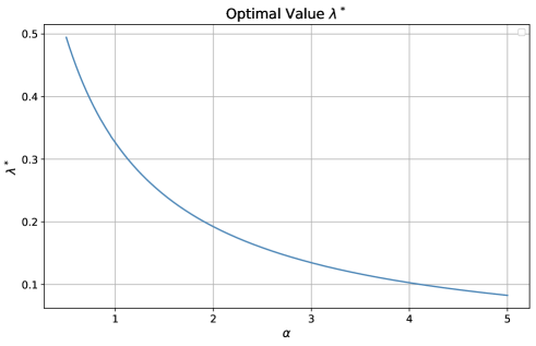
Figure 1: Optimal value of $\lambda^{*}$ with $g_{1}(x)=1-(1-x)^{2\alpha}$ and $g_{2}(x)=1-(1-x)^{3\alpha}$

Next, we analyze the case of risk-seeking agents, where $h_{i}$ and $g_{i}$ are assumed to be convex for $i\in[n]$. Intuitively, it may be reasonable to conjecture that, similarly to the risk-averse case, the group would allocate a greater proportion of their investments to risky assets if each agent becomes more risk seeking. Specifically, we aim to determine whether the inequality $\lambda_{h}\leqslant\lambda_{g}$ holds when every agent in the group becomes more risk seeking; that is, $h_{i}\geqslant g_{i}$ for each $i\in[n]$. By Proposition 4, the problem reduces to verifying whether the following relationship holds for $X\in\mathcal{X}^{\perp}$:

$$\rho_{f_{h}}(X)\leqslant\rho_{f_{g}}(X),\ \text{where}\ f_{h}(x)=\frac{\mathop{\lozenge}\displaylimits_{i=1}^{n}\tilde{h}_{i}(x)}{\mathop{\lozenge}\displaylimits_{i=1}^{n}\tilde{h}_{i}(1)}\ \text{and}\ f_{g}(x)=\frac{\mathop{\lozenge}\displaylimits_{i=1}^{n}\tilde{g}_{i}(x)}{\mathop{\lozenge}\displaylimits_{i=1}^{n}\tilde{g}_{i}(1)}.$$ (19)

Problem (19) is equivalent to determining whether $f_{h}\leqslant f_{g}$ holds on $[0,1]$ since $f_{h}$ and $f_{g}$ are distortion functions; see e.g., Wang et al., 2020b (, Lemma 1). Note that $h_{i}\geqslant g_{i}$ implies $\tilde{h}_{i}\leqslant\tilde{g}_{i}$. Also, both $\tilde{h}_{i}$ and $\tilde{h}_{i}$ are concave as $h_{i}$ and $g_{i}$ are convex. Although $\tilde{h}_{i}\leqslant\tilde{g}_{i}$ leads to $\mathop{\lozenge}\displaylimits_{i=1}^{n}\tilde{h}_{i}\leqslant\mathop{\lozenge}\displaylimits_{i=1}^{n}\tilde{g}_{i}$, the inequality $f_{h}\leqslant f_{g}$ does not necessarily hold because $f_{h}$ and $f_{g}$ are defined as ratios. To illustrate this point, we present two numerical examples. The numerical results in Example 7 align with our intuition, whereas Example 8 provides a counterexample, showing that (19) is not always true.

Example 7.

We consider a group of two risk-seeking agents and assume that their risk preferences are modeled by $\ell_{1}(x,\alpha)=1-(1-x)^{0.2\alpha}$ and $\ell_{2}(x,\alpha)=1-(1-x)^{0.3\alpha}$, respectively. We take $\alpha\in[0,3]$ to ensure the convexity of $\ell_{1}$ and $\ell_{2}$. As $\alpha$ decreases, both agents exhibit increasingly risk-seeking behavior, thus a larger optimal $\lambda^{*}$ is expected. We also assume $X\sim\mathrm{U}(0,1)$. A numerical simulation of the optimal $\lambda^{*}$ with varying values of $\alpha$ are presented in Figure 2.

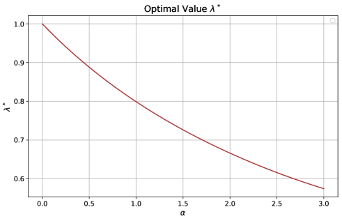
Figure 2: Optimal value of $\lambda^{*}$ with $g_{1}(x)=1-(1-x)^{0.2\alpha}$ and $g_{2}(x)=1-(1-x)^{0.3\alpha}$

In (16), taking $h_{1}(x)=\ell_{1}(x,2)$, $h_{2}(x)=\ell_{2}(x,2)$, $g_{1}(x)=\ell_{1}(x,1)$, and $g_{2}(x)=\ell_{2}(x,1)$, we have $h_{i}\geqslant g_{i}$ for $i=1,2$, and thus $\tilde{h}_{1}\mathop{\lozenge}\displaylimits\tilde{h}_{2}\leqslant\tilde{g}_{1}\mathop{\lozenge}\displaylimits\tilde{g}_{2}$, as shown in Figure 3a. In this case, it holds that $f_{h}\leqslant f_{g}$, as illustrated in Figure 3b.

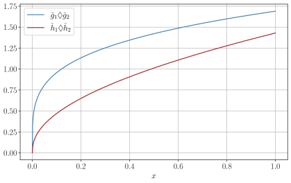
a Comparison of $\tilde{h}_{1}\mathop{\lozenge}\displaylimits\tilde{h}_{2}$ and $\tilde{g}_{1}\mathop{\lozenge}\displaylimits\tilde{g}_{2}$

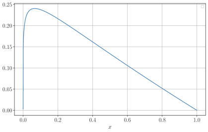
b The difference $f_{g}-f_{h}$

Figure 3: Comparison of sup-convolutions and the normalized ones in Example 7

The following counter-example shows that $f_{h}(x)>f_{g}(x)$ may occur for some $x\in(0,1)$, implying that (19) does not always hold true for a given $X$.

Example 8.

Take $h_{1}(x)=(1.24x-0.24)\vee 0$, $h_{2}(x)=(1.10x-0.1)\vee 0$ and $g_{1}(x)=(1.36x-0.36)\vee 0$, $g_{2}(x)=(1.21x-0.21)\vee 0$. Thus, it is straightforward to verify $h_{i}\geqslant g_{i}$ for $i=1,\ 2$. Also, we can obtain that $\tilde{h}_{1}(x)=(1.24x)\wedge 1$, $\tilde{h}_{2}(x)=(1.1x)\wedge 1$, and $\tilde{g}_{1}(x)=(1.36x)\wedge 1$ and $\tilde{g}_{2}(x)=(1.21x)\wedge 1$. Then we can show $\tilde{h}_{1}\mathop{\lozenge}\displaylimits\tilde{h}_{2}$ and $\tilde{g}_{1}\mathop{\lozenge}\displaylimits\tilde{g}_{2}$ have the following explicit forms

$$\tilde{h}_{1}\mathop{\lozenge}\displaylimits\tilde{h}_{2}(x)=\begin{cases}1.24x&x\in[0,0.81]\\ 1.1x+a&x\in[0.81,1];\end{cases}~~\ \tilde{g}_{1}\mathop{\lozenge}\displaylimits\tilde{g}_{2}(x)=\begin{cases}1.36x&x\in[0,0.73]\\ 1.21x+b&x\in[0.73,1].\end{cases}$$

where $a=0.14/1.24$ and $b=0.15/1.36$. Figure 4a compares two sup-convolutions, showing that $\tilde{h}_{1}\mathop{\lozenge}\displaylimits\tilde{h}_{2}\leqslant\tilde{g}_{1}\mathop{\lozenge}\displaylimits\tilde{g}_{2}$ holds over $[0,1]$. However, with normalization at 1, $f_{h}\leqslant f_{g}$ no longer holds over $[0,1]$. As shown in Figure 4b, the difference between $f_{h}$ and $f_{g}$ crosses the zero line, with $f_{h}$ exceeding $f_{g}$ beyond a certain point near 0.8.

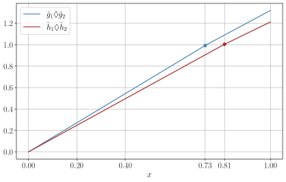
a Comparison of $\tilde{h}_{1}\mathop{\lozenge}\displaylimits\tilde{h}_{2}$ and $\tilde{g}_{1}\mathop{\lozenge}\displaylimits\tilde{g}_{2}$

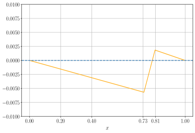
b The difference $f_{g}-f_{h}$

Figure 4: Comparison of sup-convolutions and the normalized ones in Example 8

One possible explanation of this phenomenon is that, for a group of risk-seeking agents, the overall risk they encounter stems from two sources: external randomness, introduced by a risky asset, and internal randomness, generated through counter-monotonic risk-sharing within the group, thus gambling among themselves. As agents become increasingly risk-seeking, their preference for internal randomness, arising from gambling within the group, may dominate their interest in external randomness. Recognizing this, the manager might allocate less to the external risky asset because the group is already sufficiently satisfied from their internal gambling. This strategy not only aligns with the agents’ preferences but also achieves the goal of minimizing risk exposure as a group. To explain this plainly, one may think that for a group of investors who see the stock market as a casino, they may directly go to the casino without putting much money in the stock market.

7 Conclusion

The counter-monotonic improvement theorem (reported as Theorem 1 herein) not only provides insights into solving risk sharing problem among non-risk-averse agents, but also serves as the foundation for studying a counter-monotonic risk exchange mechanism, in which only counter-monotonic risk allocations are allowed. In this paper, we investigate the counter-monotonic risk sharing problem for heterogeneous underlying risk measures $\rho_{h_{1}},\dots,\rho_{h_{n}}$.

When all agents are risk averse, meaning that $h_{i}$ is concave for each $i\in[n]$, the following relationship holds (Theorem 2 and Corollary 1):

$$\mathop{\boxminus}\displaylimits_{i=1}^{n}\rho_{h_{i}}\geqslant\mathop{\boxplus}\displaylimits_{i=1}^{n}\rho_{h_{i}}=\rho_{h}=\mathop{\square}\displaylimits_{i=1}^{n}\rho_{h_{i}},\ \text{where}\ h=\bigwedge_{i=1}^{n}h_{i}.$$

In this case, comonotonic allocations are always preferred, implying that the counter-monotonic inf-convolution generally yields a larger value than the other two. As a result, finding a closed-form characterization of the counter-monotonic inf-convolution becomes challenging, and it is not our focus in this paper. However, we provide a sufficient condition under which $\mathop{\boxminus}\displaylimits_{i=1}^{n}\rho_{h_{i}}$ is equal to the other two inf-convolutions.

When $h_{i}$ is convex and continuous on $[0,1]$ for each $i\in[n]$, indicating that agents are risk seeking, the inf-convolution for such distortion risk measures admits explicit formulas for $X\in\mathcal{X}^{\perp}$:

$$\mathop{\square}\displaylimits_{i=1}^{n}\rho_{h_{i}}(X)=\mathop{\boxminus}\displaylimits_{i=1}^{n}\rho_{h_{i}}(X)=\rho_{g}(X),$$

where $g$ is such that (i) $g=\mathop{\square}\displaylimits_{i=1}^{n}h_{i}$ if $\mathcal{X}=L^{+}$; and (ii) $\tilde{g}=\mathop{\lozenge}\displaylimits_{i=1}^{n}\tilde{h}_{i}$ if $\mathcal{X}=L^{-}$. In this setting, these results show that a representative agent (defined by the inf-convolution as its reference) of several agents with distortion risk measures is no longer an agent with a distortion risk measure, but rather with a distortion riskmetric.

Combining the results for risk-averse agents and risk-seeking agents, we are able to solve a portfolio manager’s problem in which the optimal investment strategies are determined explicitly (Proposition 4). A counterintuitive observation from these results is that when all agents in a group become more risk seeking, increasing the allocation to risky investments is not always the optimal strategy for the manager. This finding naturally raises the question of identifying the conditions under which such a strategy is optimal, specifically when (19) holds. Exploring this question would be a promising direction for future work, focusing on the comparison of risk-seeking behaviors across groups.

References

- Acciaio, (2007) Acciaio, B. (2007). Optimal risk sharing with non-monotone monetary functionals. Finance and Stochastics, 11:267–289.
- Artzner et al., (1999) Artzner, P., Delbaen, F., Eber, J.-M., and Heath, D. (1999). Coherent measures of risk. Mathematical Finance, 9(3):203–228.
- Barrieu and El Karoui, (2005) Barrieu, P. and El Karoui, N. (2005). Inf-convolution of risk measures and optimal risk transfer. Finance and Stochastics, 9(2):269–298.
- Beißner and Werner, (2023) Beißner, P. and Werner, J. (2023). Optimal allocations with -maxmin utilities, choquet expected utilities, and prospect theory. Theoretical Economics, 18(3):993–1022.
- Boonen et al., (2021) Boonen, T. J., Liu, F., and Wang, R. (2021). Competitive equilibria in a comonotone market. Economic Theory, 72(4):1217–1255.
- Borch, (1962) Borch, K. (1962). Equilibrium in a reinsurance market. Econometrica, 30(3):424–444.
- Carlier et al., (2012) Carlier, G., Dana, R.-A., and Galichon, A. (2012). Pareto efficiency for the concave order and multivariate comonotonicity. Journal of Economic Theory, 147(1):207–229.
- Chaoubi et al., (2020) Chaoubi, I., Cossette, H., Gadoury, S.-P., and Marceau, E. (2020). On sums of two counter-monotonic risks. Insurance: Mathematics and Economics, 92:47–60.
- Chateauneuf et al., (2000) Chateauneuf, A., Dana, R. A., and Tallon, J. M. (2000). Optimal risk-sharing rules and equilibria with choquet-expected-utility. Journal of Mathematical Economics, 34(2):191–214.
- Cheung et al., (2014) Cheung, K. C., Dhaene, J., Lo, A., and Tang, Q. (2014). Reducing risk by merging counter-monotonic risks. Insurance: Mathematics and Economics, 54:58–65.
- Cheung and Lo, (2014) Cheung, K. C. and Lo, A. (2014). Characterizing mutual exclusivity as the strongest negative multivariate dependence structure. Insurance: Mathematics and Economics, 55:180–190.
- Dall’Aglio, (1972) Dall’Aglio, G. (1972). Fréchet classes and compatibility of distribution functions. Symposia mathematica, 9:131–150.
- Dana, (2002) Dana, R. A. (2002). On equilibria when agents have multiple priors. Annals of Operations Research, 114(1):105–115.
- Dana, (2004) Dana, R. A. (2004). Ambiguity, uncertainty aversion and equilibrium welfare. Economic Theory, 23:569–587.
- De Castro and Chateauneuf, (2011) De Castro, L. I. and Chateauneuf, A. (2011). Ambiguity aversion and trade. Economic Theory, 48:243–273.
- Denneberg, (1994) Denneberg, D. (1994). Non-additive measure and integral. Springer Science & Business Media.
- Denuit et al., (2025) Denuit, M., Dhaene, J., Ghossoub, M., and Robert, C. (2025). Comonotonicity and Pareto Optimality with Application to Collaborative Insurance. Insurance: Mathematics and Economics, 120(1):1–16.
- Dhaene and Denuit, (1999) Dhaene, J. and Denuit, M. (1999). The safest dependence structure among risks. Insurance: Mathematics and Economics, 25(1):11–21.
- Dhaene et al., (2002) Dhaene, J., Denuit, M., Goovaerts, M. J., Kaas, R., and Vyncke, D. (2002). The concept of comonotonicity in actuarial science and finance: Theory. Insurance: Mathematics and Economics, 31(1):3–33.
- Dhaene et al., (2006) Dhaene, J., Vanduffel, S., Goovaerts, M. J., Kaas, R., Tang, Q., and Vyncke, D. (2006). Risk measures and comonotonicity: a review. Stochastic models, 22(4):573–606.
- Embrechts et al., (2020) Embrechts, P., Liu, H., Mao, T., and Wang, R. (2020). Quantile-based risk sharing with heterogeneous beliefs. Mathematical Programming, 181:319–347.
- Embrechts et al., (2018) Embrechts, P., Liu, H., and Wang, R. (2018). Quantile-based risk sharing. Operations Research, 66(4):936–949.
- Filipović and Svindland, (2008) Filipović, D. and Svindland, G. (2008). Optimal capital and risk allocations for law-and cash-invariant convex functions. Finance and Stochastics, 12:423–439.
- Föllmer and Schied, (2016) Föllmer, H. and Schied, A. (2016). Stochastic finance: An introduction in discrete time. Walter de Gruyter.
- (25) Ghossoub, M., Ren, Q., and Wang, R. (2024a). Counter-monotonic risk allocations and distortion risk measures. arXiv preprint arXiv:2407.16099.
- Ghossoub and Zhu, (2024) Ghossoub, M. and Zhu, M. B. (2024). Efficiency in pure-exchange economies with risk-averse monetary utilities. arXiv preprint arXiv:2406.02712.
- (27) Ghossoub, M., Zhu, M. B., and Chong, W. F. (2024b). Pareto-optimal peer-to-peer risk sharing with robust distortion risk measures. arXiv preprint arXiv:2409.05103.
- Guan et al., (2024) Guan, Y., Jiao, Z., and Wang, R. (2024). A reverse ES (CVaR) optimization formula. North American Actuarial Journal, 28(3):611–625.
- He et al., (2016) He, J., Tang, Q., and Zhang, H. (2016). Risk reducers in convex order. Insurance: Mathematics and Economics, 70:80–88.
- Jouini et al., (2008) Jouini, E., Schachermayer, W., and Touzi, N. (2008). Optimal risk sharing for law invariant monetary utility functions. Mathematical Finance, 18(2):269–292.
- Landsberger and Meilijson, (1994) Landsberger, M. and Meilijson, I. (1994). Co-monotone allocations, bickel-lehmann dispersion and the arrow-pratt measure of risk aversion. Annals of Operations Research, 52:97–106.
- (32) Lauzier, J. G., Lin, L., and Wang, R. (2023a). Pairwise counter-monotonicity. Insurance: Mathematics and Economics, 111:279–287.
- (33) Lauzier, J. G., Lin, L., and Wang, R. (2023b). Risk sharing, measuring variability, and distortion riskmetrics. arXiv preprint arXiv:2302.04034.
- Lauzier et al., (2024) Lauzier, J. G., Lin, L., and Wang, R. (2024). Negatively dependent optimal risk sharing. arXiv preprint arXiv:2401.03328.
- Liebrich, (2024) Liebrich, F.-B. (2024). Risk sharing under heterogeneous beliefs without convexity. Finance and Stochastics, 28(4):999–1033.
- Liu, (2020) Liu, H. (2020). Weighted comonotonic risk sharing under heterogeneous beliefs. ASTIN Bulletin: The Journal of the IAA, 50(2):647–673.
- Ludkovski and Rüschendorf, (2008) Ludkovski, M. and Rüschendorf, L. (2008). On comonotonicity of pareto optimal risk sharing. Statistics & Probability Letters, 78(10):1181–1188.
- Mastrogiacomo and Rosazza Gianin, (2015) Mastrogiacomo, E. and Rosazza Gianin, E. (2015). Pareto optimal allocations and optimal risk sharing for quasiconvex risk measures. Mathematics and Financial Economics, 9(2):149–167.
- Phillips, (2003) Phillips, G. M. (2003). Interpolation and approximation by polynomials. Springer Science & Business Media.
- Principi et al., (2023) Principi, G., Wakker, P. P., and Wang, R. (2023). Antimonotonicity for preference axioms: The natural counterpart to comonotonicity. arXiv preprint arXiv:2307.08542.
- Ravanelli and Svindland, (2014) Ravanelli, C. and Svindland, G. (2014). Pareto Optimal Allocations for Law Invariant Robust Utilities on . Finance and Stochastics, 18:249–269.
- Rothschild and Stiglitz, (1970) Rothschild, M. and Stiglitz, J. (1970). Increasing Risk: I. A Definition. Journal of Economic Theory, 2(3):225–243.
- Rüschendorf, (2013) Rüschendorf, L. (2013). Mathematical risk analysis. Springer.
- Schmeidler, (1989) Schmeidler, D. (1989). Subjective probability and expected utility without additivity. Econometrica, 57:571–587.
- Tsanakas and Christofides, (2006) Tsanakas, A. and Christofides, N. (2006). Risk exchange with distorted probabilities. ASTIN Bulletin: The Journal of the IAA, 36(1):219–243.
- (46) Wang, Q., Wang, R., and Wei, Y. (2020a). Distortion riskmetrics on general spaces. ASTIN Bulletin: The Journal of the IAA, 50(3):827–851.
- (47) Wang, R., Wei, Y., and Willmot, G. E. (2020b). Characterization, robustness, and aggregation of signed choquet integrals. Mathematics of Operations Research, 45(3):993–1015.
- Weber, (2018) Weber, S. (2018). Solvency ii, or how to sweep the downside risk under the carpet. Insurance: Mathematics and Economics, 82:191–200.
- Wilson, (1968) Wilson, R. (1968). The theory of syndicates. Econometrica, 36:119–132.