Quantum algorithm for unstructured search of ranked targets

Abstract

Grover’s quantum algorithm can find a marked item from an unstructured database faster than any classical algorithm, and hence it has been used for several applications such as cryptanalysis and optimization. When there exist multiple marked items, Grover’s algorithm has the property of finding one of them uniformly at random. To further broaden the application range, it was generalized so that it finds marked items with probabilities according to their priority by encoding the priority into amplitudes applied by Grover’s oracle operator. In this paper, to achieve a similar generalization, we examine a different encoding that incorporates the priority into phases applied by the oracle operator. We compare the previous and our oracle operators and observe that which one performs better depends on priority parameters. Since the priority parameters can be considered as the magnitude of the correlated phase error on Grover’s oracle operator, the analysis of our oracle operator also reveals the robustness of the original Grover’s algorithm against correlated noises. We further numerically show that the coherence between multiple marked items increases the probability of finding the most prioritized one in Grover’s algorithm with our oracle operator.

Keywords: quantum computation, Grover’s algorithm, priority

I Introduction

Several quantum algorithms (e.g., DJ92 ; K95 ; G97 ; Si97 ; S97 ; HHL09 ; MNRS11 ; LGZ16 ; MRTC21 ) superior to classical ones have been proposed, and some of them were already demonstrated in small scale experiments CGK98 ; CVZLL98 ; JMH98 ; VSBYSC01 ; WRRSWVAZ05 ; HRBPK06 ; ZSCXLGZXDHWYZLPWLZ17 ; RDSD24 . Among them, Grover’s algorithm G97 (for details, see Sec. II) is especially attractive due to its versatility. It has been applied to numerous applications such as collision and claw finding BHT98 , machine learning WNHT20 ; DHLT21 , and optimization BBW03 ; BBW05 ; DHHM06 ; BE20 . Grover’s algorithm finds a marked item from an unstructured database quadratically faster than any classical algorithm G97 ; G96 and is optimal in the sense that the dependence of its query complexity on the database size and the number of marked items cannot be improved any further BBBV97 ; BBHT99 . Here, query complexity is the number of accesses to the database.

To further broaden the application range, Grover’s algorithm has been improved and generalized in various directions. The success probability of the original Grover’s algorithm, i.e., the probability of finding a marked item is close to one, but it is strictly less than one except for the special case. This issue was solved in Refs. H00 ; L01 ; BHMT02 ; RJS22 ; RJS23 by proposing a modified Grover’s algorithm that can find a marked item without failure. A method of reducing the failure probability to any non-zero small value was also devised in Ref. BCWZ99 . Another property of the original Grover’s algorithm is that when there exist multiple marked items in the unstructured database, it outputs one of them uniformly at random, which would imply that the original Grover’s algorithm cannot take the priority of the multiple marked items into consideration. Panchi and Shiyong modified Grover’s oracle operator so that the marked items are output with probabilities according to their priority PS08 . More specifically, they encoded the priority into amplitudes applied by Grover’s oracle operator [see Eq. (38)]. Grover’s algorithm with their modified oracle operator was applied to the cluster head selection in wireless sensor networks RK23 .

In this paper, we propose another quantum algorithm for unstructured search with priority. As a difference from the algorithm in Ref. PS08 , we use a phase encoding rather than the amplitude encoding. In the original Grover’s algorithm, the phase $-1$ is applied to every marked items by the oracle operator. On the other hand, our oracle operator applies $-e^{i\pi\epsilon_{i}}$ to the $i$th marked item, where $-1\leq\epsilon_{i}\leq 0$ is the priority parameter. Since when $\epsilon_{i}=0$ for all $i$, our oracle operator becomes the original Grover’s one, Grover’s algorithm with our oracle operator can be considered as a generalization of the original Grover’s algorithm. To clarify which of the phase and amplitude encoding is better for taking the priority into account, we numerically compare our oracle operator and that in Ref. PS08 under the condition that there exist two marked items. As a result, we observe that when a marked item is highly prioritized than another one, our oracle operator would be superior to the existing one. On the other hand, when the two marked items are similarly prioritized, the existing algorithm becomes better than ours (for details, see Sec. III.4). We further numerically show that the coherence between the two marked items increases the probability of finding the most prioritized one in Grover’s algorithm with our oracle operator.

The analysis of our oracle operator is also related to the robustness of the original Grover’s algorithm against correlated phase errors. This is because the absolute value $|\epsilon_{i}|$ of the priority parameter can be considered as the noise strength on the oracle operator. Furthermore, each marked item is basically represented by multiple qubits, and the absolute value of its priority parameter can depend on all the qubits, and hence we call our errors correlated ones. As with our analysis, several noise effects on Grover’s algorithm have been investigated by considering noisy oracle operators. Remarkably, when the oracle operator does not work with an arbitrarily small constant probability, the quadratic speed-up of Grover’s algorithm is completely canceled RS08 . The similar results were also shown for the depolarizing and dephasing noises R23 . However, this cancellation does not always occur, and a concrete noise model where the quadratic speed-up survives was found HMW03 . Our noise model was also already investigated under the restriction that there is only a single marked item LLZT20 ; SBW03 , that the noise strength is the same for all marked items LSZN99 ; LL07 ; TDNTK08 ; TD24 , or that the noise strength is randomly chosen from $\{-1,0\}$ ABNR12 ; KNR18 . Particularly, Refs. TDNTK08 ; TD24 consider a realistic situation where the noise strength changes every time the oracle operator is applied. As another noise model, a systematic noise that causes coherent errors was also investigated DZKK24 . Our results, together with these existing results, would deepen the understanding on the noise robustness of Grover’s algorithm.

II Grover’s algorithm

Since our oracle operator is constructed by modifying Grover’s oracle operator, we first review the original Grover’s algorithm G97 ; LMP03 . For a given function $f:\mathcal{X}\equiv\{0,1,\ldots,n-1\}\rightarrow\{0,1\}$ with a natural number $n$, its purpose is to find a marked item $x\in\mathcal{X}$ satisfying $f(x)=1$. It is worth mentioning that such $x$ is, in general, not unique GK17 . Let $m\equiv\sum_{x\in\mathcal{X}}f(x)$ be the number of $x$’s satisfying $f(x)=1$. For simplicity, we assume $1\leq m\ll n$ in this section. To find a marked item (with a sufficiently high probability), any classical algorithm requires $\Omega(n/m)$ queries to an oracle for $f$ in the worst case. On the other hand, Grover’s algorithm can do the same thing with only $O(\sqrt{n/m})$ quantum queries.

Grover’s algorithm proceeds as follows:

1. Prepare the initial state

   $$|\psi(0)\rangle\equiv\cfrac{1}{\sqrt{n}}\sum_{x=0}^{n-1}|x\rangle.$$ (1)

2. Apply the unitary operator $G\equiv DO_{f}$ to the initial state in Eq. (1) $t$ times, where

   $$D\equiv 2|\psi(0)\rangle\langle\psi(0)|-I^{(n)}$$ (2)

   is Grover’s diffusion operator, $I^{(d)}$ is the $d$-dimensional identity operator for any natural number $d$, and

   $$O_{f}\equiv I^{(n)}-2\sum_{x\in\mathcal{X}_{1}}|x\rangle\langle x|$$ (3)

   is the oracle operator. Here, $\mathcal{X}_{b}\equiv\{x|x\in\mathcal{X},f(x)=b\}$, and hence $\mathcal{X}_{0}\cup\mathcal{X}_{1}=\mathcal{X}$, and $\mathcal{X}_{0}\cap\mathcal{X}_{1}=\varnothing$. At the end of this step, the state is

   $$|\psi(t)\rangle\equiv G^{t}|\psi(0)\rangle.$$ (4)

3. Measure the final state $|\psi(t)\rangle$ in the computational basis $\{|x\rangle\}_{x\in\mathcal{X}}$.

4. Output the measurement outcome $x$ as a solution.

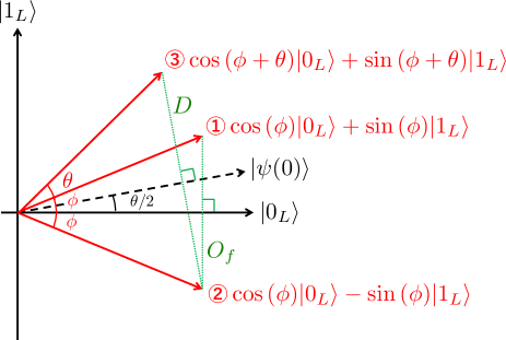
Figure 1: Geometric interpretation of $G\equiv DO_{f}$. The oracle operator $O_{f}$ transforms $\cos{(\phi)}|0_{L}\rangle+\sin{(\phi)}|1_{L}\rangle$ to the quantum state in Eq. (8) for any real number $\phi$, which can be interpreted as the reflection along the horizontal axis $|0_{L}\rangle$. Grover’s diffusion operator $D$ transforms the quantum state in Eq. (8) to that in Eq. (9). It is interpreted as the reflection along the dotted axis corresponding to the initial state $|\psi(0)\rangle$. These interpretations imply that $|\psi(0)\rangle$ gets close to the superposition $|1_{L}\rangle$ of marked items by repeating the implementation of $G$.

The query to the oracle for $f$ is implemented with the oracle operator $O_{f}$ because it multiplies $(-1)^{f(x)}$ to $|x\rangle$. Therefore, the query complexity of Grover’s algorithm is the number $t$ of uses of $O_{f}$. We derive $t=O(\sqrt{n/m})$ by using a geometric interpretation of $G$ given in Fig. 1. Although Grover’s algorithm uses multiple qubits (more precisely, $O(\log{n})$ qubits), its behaviour can be captured as a quantum algorithm running on a single logical qubit with the orthonormal basis

$$\left\{|0_{L}\rangle\equiv\cfrac{1}{\sqrt{n-m}}\sum_{x\in\mathcal{X}_{0}}|x\rangle,|1_{L}\rangle\equiv\cfrac{1}{\sqrt{m}}\sum_{x\in\mathcal{X}_{1}}|x\rangle\right\}.$$ (5)

By using the basis in Eq. (5), the initial state in Eq. (1) is rewritten as

$$|\psi(0)\rangle=\cos{\left(\cfrac{\theta}{2}\right)}|0_{L}\rangle+\sin{\left(\cfrac{\theta}{2}\right)}|1_{L}\rangle,$$ (6)

where $0<\theta<\pi$, and

$$\theta\equiv 2\sin^{-1}{\left(\sqrt{\cfrac{m}{n}}\right)}\simeq 2\sqrt{\cfrac{m}{n}}.$$ (7)

Here, the last approximation comes from the assumption that $m\ll n$. On the other hand, the direct calculation shows that

$$O_{f}\left[\cos{(\phi)}|0_{L}\rangle+\sin{(\phi)}|1_{L}\rangle\right]=\cos{(\phi)}|0_{L}\rangle-\sin{(\phi)}|1_{L}\rangle$$ (8)

for any real number $\phi$. Then, Grover’s diffusion operator $D$ transforms the quantum state in Eq. (8) to

$$DO_{f}\left[\cos{(\phi)}|0_{L}\rangle+\sin{(\phi)}|1_{L}\rangle\right]=\cos{(\phi+\theta)}|0_{L}\rangle+\sin{(\phi+\theta)}|1_{L}\rangle.$$ (9)

The transformations in Eqs. (8) and (9) can be interpreted as the reflections in Fig. 1. This geometrical interpretation implies that the angle $\theta$ is added every time we apply $G$, and thus the final state of Grover’s algorithm is

$$|\psi(t)\rangle=\cos{\left(\cfrac{2t+1}{2}\theta\right)}|0_{L}\rangle+\sin{\left(\cfrac{2t+1}{2}\theta\right)}|1_{L}\rangle.$$ (10)

The success probability (i.e., the probability of obtaining $x$ satisfying $f(x)=1$ in step 3) $\sin^{2}{((2t+1)\theta/2)}$ is maximized when

$$t=\left\lfloor\cfrac{\pi}{2\theta}\right\rfloor=O\left(\sqrt{\cfrac{n}{m}}\right)$$ (11)

with $\lfloor\cdot\rfloor$ being the floor function. Note that in the exceptional case of $\pi/(2\theta)$ being an integer, $t=\lfloor\pi/(2\theta)\rfloor-1$ also maximizes the success probability.

It is worth mentioning that since $|1_{L}\rangle$ is the equal superposition of $m$ marked items [see Eq. (5)], Grover’s algorithm outputs each correct answer with the same probability

$$\cfrac{\sin^{2}{\left(\left(\left\lfloor\cfrac{\pi}{2\theta}\right\rfloor+\cfrac{1}{2}\right)\theta\right)}}{m}\simeq\cfrac{1}{m}.$$ (12)

Our subject in this paper is to bias the probability distribution to reflect the priority of each answer by modifying the oracle operator in Eq. (3).

III Generalized Grover’s algorithm with ranked targets

In this section, we give our main results. In Sec. III.1, we explain the behaviour of Grover’s algorithm for our oracle operator and numerically evaluate it. In Sec. III.2, we give an analytical evaluation of our oracle operator under a concrete condition. As a result, we show that its success probability can be calculated by solving a cubic equation. We also obtain a sufficient condition for that the most prioritized items are more frequently observed than the other items by deriving approximations of success probabilities of Grover’s algorithm with our oracle operator. In Sec. III.3, we consider the case of $m=2$ and numerically observe that the coherence between the two marked items increases the probability of finding the most prioritized one in Grover’s algorithm with our oracle operator. In this sense, our oracle operator effectively uses the quantum effect. In Sec. III.4, we compare our oracle operator with that in Ref. PS08 .

III.1 Unstructured search of ranked targets

As stated in Sec. II, the original Grover’s algorithm treats all marked items equally. However, in general, some of the marked items may be prioritized than the others. For example, when a given oracle can only decide the likelihood that an input $x$ satisfies $f(x)=1$, the marked items would be ranked depending on their likelihood. As stated in Sec. I, the same situation arises also when the oracle operator is affected by correlated phase errors. Our purpose is to devise a quantum algorithm that finds the marked items with probabilities according to their priority. More formally, let $-1\leq\epsilon_{x}\leq 0$ be a priority parameter for any marked item $x\in\mathcal{X}_{1}$. When two marked items $x$ and $y$ satisfy $\epsilon_{x}>\epsilon_{y}$, we would like to find $x$ with a higher probability than that of $y$.

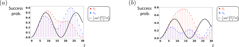
Figure 2: Success probabilities of our quantum algorithm. In this figure, we set $n=256$, $m=2$, and $\epsilon_{\tilde{x}_{1}}=0$. The red and blue dotted curves represent $P_{\rm suc}^{(\tilde{x}_{1})}(\vec{\epsilon},t)$ and $P_{\rm suc}^{(\tilde{x}_{2})}(\vec{\epsilon},t)$, respectively. The black curves correspond to the probability $\sin^{2}{((2t+1)\theta/2)}/m$ of the original Grover’s algorithm finding a single marked item $\tilde{x}_{1}$ or $\tilde{x}_{2}$. (a) The case of $\epsilon_{\tilde{x}_{2}}=-0.05$. (b) The case of $\epsilon_{\tilde{x}_{2}}=-0.1$.

To this end, we replace the oracle operator $O_{f}$ in Eq. (3) with

$$\tilde{O}_{f}(\vec{\epsilon})\equiv I^{(n)}-\sum_{x\in\mathcal{X}_{1}}(1+e^{i\pi\epsilon_{x}})|x\rangle\langle x|,$$ (13)

where $\vec{\epsilon}\equiv{(\epsilon_{x})}_{x\in\mathcal{X}_{1}}$. By definition, it is trivial that $\tilde{O}_{f}(\vec{\epsilon})$ becomes the original oracle operator $O_{f}$ when $\epsilon_{x}=0$ holds for all $x\in\mathcal{X}_{1}$. Therefore, we can say that our oracle operator is a generalization of Grover’s oracle operator. Our quantum algorithm is the same as Grover’s algorithm except for that the oracle operator is replaced with $\tilde{O}_{f}(\vec{\epsilon})$, and hence the final state of our algorithm is

$$|\tilde{\psi}(\vec{\epsilon},t)\rangle\equiv\left[D\tilde{O}_{f}(\vec{\epsilon})\right]^{t}|\psi(0)\rangle.$$ (14)

For any $1\leq i\leq m$, we define $\tilde{x}_{i}$ and $P_{\rm suc}^{(\tilde{x}_{i})}(\vec{\epsilon},t)\equiv|\langle\tilde{x}_{i}|\tilde{\psi}(\vec{\epsilon},t)\rangle|^{2}$ as the $i$th marked item and the probability of obtaining $\tilde{x}_{i}$ in our quantum algorithm, respectively.

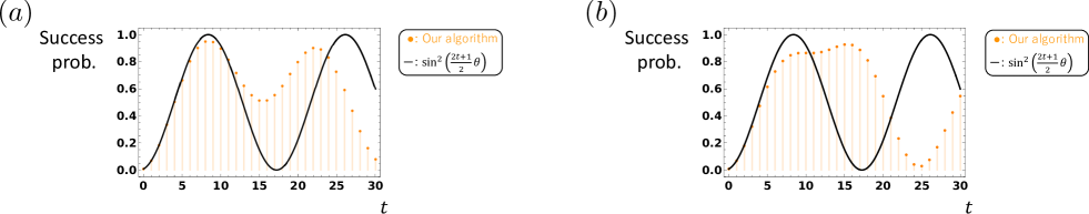
Figure 3: Overall success probabilities of our quantum algorithm. In this figure, we set $n=256$, $m=2$, and $\epsilon_{\tilde{x}_{1}}=0$. The orange dotted curves represent $\sum_{x\in\mathcal{X}_{1}}P_{\rm suc}^{(x)}(\vec{\epsilon},t)$. The black curves correspond to the overall success probability $\sin^{2}{((2t+1)\theta/2)}$ of the original Grover’s algorithm. (a) The case of $\epsilon_{\tilde{x}_{2}}=-0.05$. (b) The case of $\epsilon_{\tilde{x}_{2}}=-0.1$.

To show, in a tangible way, that our quantum algorithm correctly prioritizes marked items, we perform several numerical simulations with $n=256$, $m=2$, and $\epsilon_{\tilde{x}_{1}}=0$. The first numerical simulation is given in Fig. 2. It reveals that the first marked item $\tilde{x}_{1}$ with the highest priority parameter $\epsilon_{\tilde{x}_{1}}=0$ is more frequently observed than the second marked item $\tilde{x}_{2}$ with a lower priority parameter $\epsilon_{\tilde{x}_{2}}<0$ by choosing an appropriate $t$ such as $\lfloor\pi/(2\theta)\rfloor=8$ [see Eq. (11)]. More concretely, compared with the original Grover’s algorithm, the observation of $\tilde{x}_{1}$ is facilitated, but that of $\tilde{x}_{2}$ is suppressed. On the other hand, at inappropriate values of $t$ such as $t=30$, $\tilde{x}_{2}$ is more frequently observed than $\tilde{x}_{1}$. To avoid this unfavourable situation, we will give an analytical sufficient condition on $t$ in Sec. III.2 under the assumption that $|\epsilon_{\tilde{x}_{2}}|$ is sufficiently small but not $0$. It is also worth mentioning that the unfavourable situation may disappear by increasing the database size $n$ (see Fig. 6). We then compare the overall success probability $\sum_{x\in\mathcal{X}_{1}}P_{\rm suc}^{(x)}(\vec{\epsilon},t)$ of our algorithm with that of the original Grover’s algorithm in Fig. 3. From this comparison, we can deduce that the priority is yielded by sacrificing the overall success probability.

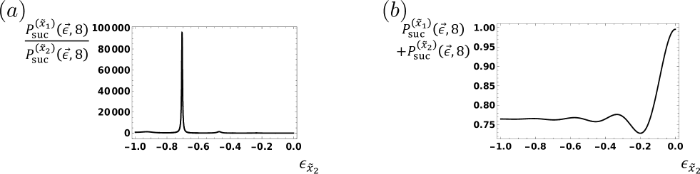
Figure 4: Dependence of our quantum algorithm on $\epsilon_{\tilde{x}_{2}}$. In this figure, we set $n=256$, $m=2$, $\epsilon_{\tilde{x}_{1}}=0$, and $t=\lfloor\pi/(2\theta)\rfloor=8$. (a) The ratio of $P_{\rm suc}^{(\tilde{x}_{1})}(\vec{\epsilon},8)$ to $P_{\rm suc}^{(\tilde{x}_{2})}(\vec{\epsilon},8)$. (b) The overall success probability $\sum_{i=1}^{2}P_{\rm suc}^{(\tilde{x}_{i})}(\vec{\epsilon},8)$.

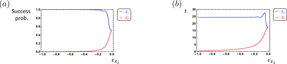
Figure 5: Dependence of our quantum algorithm on $\epsilon_{\tilde{x}_{2}}$. In this figure, we set $n=1000$, $m=2$, and $\epsilon_{\tilde{x}_{1}}=0$. (a) The first local maximum values of the success probabilities $P_{\rm suc}^{(\tilde{x}_{1})}(\vec{\epsilon},t)$ and $P_{\rm suc}^{(\tilde{x}_{2})}(\vec{\epsilon},t)$ over $t$. The blue and red curves correspond to $\tilde{x}_{1}$ and $\tilde{x}_{2}$, respectively. (b) The numbers $t$ of queries such that $P_{\rm suc}^{(\tilde{x}_{1})}(\vec{\epsilon},t)$ and $P_{\rm suc}^{(\tilde{x}_{2})}(\vec{\epsilon},t)$ take the first local maxima. The blue and red curves correspond to $\tilde{x}_{1}$ and $\tilde{x}_{2}$, respectively.

To evaluate the flexibility of our quantum algorithm, we next calculate the ratio $P_{\rm suc}^{(\tilde{x}_{1})}(\vec{\epsilon},8)/P_{\rm suc}^{(\tilde{x}_{2})}(\vec{\epsilon},8)$ and the overall success probability $\sum_{i=1}^{2}P_{\rm suc}^{(\tilde{x}_{i})}(\vec{\epsilon},8)$ while varying $\epsilon_{\tilde{x}_{2}}$ from $-1$ to $0$. The ratio represents to what extent we can prioritize the two marked items by using our quantum algorithm. As seen from Fig. 2, $P_{\rm suc}^{(\tilde{x}_{1})}(\vec{\epsilon},t)$ and $P_{\rm suc}^{(\tilde{x}_{2})}(\vec{\epsilon},t)$ take the first local maxima at different $t$, and hence we cannot uniquely determine the optimal value of $t$. This is why we tentatively adopt the original Grover’s query complexity $t=\lfloor\pi/(2\theta)\rfloor=8$. The result of this calculation is given in Fig. 4. From Fig. 4(a), we can observe that the ratio $P_{\rm suc}^{(\tilde{x}_{1})}(\vec{\epsilon},8)/P_{\rm suc}^{(\tilde{x}_{2})}(\vec{\epsilon},8)$ becomes $1$ and $95764.3$ when $\epsilon_{\tilde{x}_{2}}$ is $0$ and $-0.704696$, respectively. Despite this high flexibility, our algorithm keeps the high overall success probability larger than $0.72$ [see Fig. 4(b)]. In other words, by considering $|\epsilon_{\tilde{x}_{2}}|$ as the noise strength, this figure implies that Grover’s algorithm is robust against correlated phase errors.

We investigate our algorithm in more detail by increasing the database size to $n=1000$ and clarifying a difference between each marked item. In Fig. 5(a), we first numerically derive the $\epsilon_{\tilde{x}_{2}}$-dependence of the first local maximum values of the success probabilities $P_{\rm suc}^{(\tilde{x}_{1})}(\vec{\epsilon},t)$ and $P_{\rm suc}^{(\tilde{x}_{2})}(\vec{\epsilon},t)$ over $t$. We notice that the probability of finding the first marked item $\tilde{x}_{1}$ becomes close to $1$ and almost invariant when $\epsilon_{\tilde{x}_{2}}\lesssim-0.2$. This would also be a circumstantial evidence that the original Grover’s algorithm is robust against correlated phase errors. Furthermore, since the point corresponding to $\epsilon_{\tilde{x}_{2}}=0$ [i.e., the intersection of the red and blue lines in Fig. 5(a)] represents the half of the success probability of the original Grover’s algorithm, our algorithm enhances the observation of $\tilde{x}_{1}$ but suppresses that of $\tilde{x}_{2}$. This is consistent with Fig. 2 because the first local maximum values of the red and blue curves are larger and smaller than those of the black curves, respectively. Similarly, in Fig. 5(b), we give the $\epsilon_{\tilde{x}_{2}}$-dependence of the query complexity $t$ such that $P_{\rm suc}^{(\tilde{x}_{1})}(\vec{\epsilon},t)$ and $P_{\rm suc}^{(\tilde{x}_{2})}(\vec{\epsilon},t)$ take the first local maxima. We can observe essentially the same behaviour as that of Fig. 5(a). That is, the query complexity corresponding to $\tilde{x}_{1}$ (i.e., the blue line) becomes almost invariant when $\epsilon_{\tilde{x}_{2}}\lesssim-0.2$, and the query complexity corresponding $\tilde{x}_{1}$ and $\tilde{x}_{2}$ are increased and decreased compared with that of the original Grover’s algorithm [i.e., the intersection of the red and blue lines in Fig. 5(b)], respectively. This figure also shows that $P_{\rm suc}^{(\tilde{x}_{1})}(\vec{\epsilon},t)$ and $P_{\rm suc}^{(\tilde{x}_{2})}(\vec{\epsilon},t)$ take the first local maxima at different values of $t$ when $\epsilon_{\tilde{x}_{2}}\neq 0$, and hence the success probabilities corresponding to the blue and red lines in Fig. 5(a) are not simultaneously achieved.

III.2 Analytical evaluation

In this section, we analytically evaluate our quantum algorithm. As an issue to be solved, the geometrical interpretation shown in Fig. 1 does not work because of the modification on the oracle operator in Eq. (13). Therefore, we introduce a different approach to obtain the final state $|\tilde{\psi}(\vec{\epsilon},t)\rangle$ based on the diagonalization of $D\tilde{O}_{f}(\vec{\epsilon})$. Although our approach is applicable to the general scenario, for simplicity, we particularly consider the situation that marked items can be divided into two sets $\mathcal{X}_{1,0}$ and $\mathcal{X}_{1,\tilde{\epsilon}}$ such that (i) $\forall x\in\mathcal{X}_{1,0}$, the value of the priority parameter is $\epsilon_{x}=0$, (ii) $\forall x\in\mathcal{X}_{1,\tilde{\epsilon}}$, the value of the priority parameter is $\epsilon_{x}=\tilde{\epsilon}$, and (iii) the cardinarities of the two sets are equal, i.e., $|\mathcal{X}_{1,0}|=|\mathcal{X}_{1,\tilde{\epsilon}}|=m/2$. It is trivial that $\mathcal{X}_{1,0}\cup\mathcal{X}_{1,\tilde{\epsilon}}=\mathcal{X}_{1}$ and $\mathcal{X}_{1,0}\cap\mathcal{X}_{1,\tilde{\epsilon}}=\varnothing$ hold. This situation is not general but includes all the situations considered in Sec. III.1.

In this case, our oracle operator in Eq. (13) becomes

$$\tilde{O}_{f}(\tilde{\epsilon})=I^{(n)}-2\sum_{x\in\mathcal{X}_{1,0}}|x\rangle\langle x|-\left(1+e^{i\pi\tilde{\epsilon}}\right)\sum_{x\in\mathcal{X}_{1,\tilde{\epsilon}}}|x\rangle\langle x|.$$ (15)

By following the idea in Sec. II, we introduce the three logical basis states as follows:

$$|1^{\prime}_{L}\rangle\equiv\sqrt{\cfrac{2}{m}}\sum_{x\in\mathcal{X}_{1,0}}|x\rangle,$$ (16)

$$|1^{\prime\prime}_{L}\rangle\equiv\sqrt{\cfrac{2}{m}}\sum_{x\in\mathcal{X}_{1,\tilde{\epsilon}}}|x\rangle,$$ (17)

and $|0_{L}\rangle$ in Eq. (5). The quantum state during the execution of our algorithm can be written as a superposition of these basis states. In fact, the initial state, Grover’s diffusion operator, and our oracle operator are rewritten as

$$|\psi(0)\rangle=\cos{\left(\cfrac{\theta}{2}\right)}|0_{L}\rangle+\sin{\left(\cfrac{\theta}{2}\right)}\cfrac{|1^{\prime}_{L}\rangle+|1^{\prime\prime}_{L}\rangle}{\sqrt{2}}=\cfrac{1}{\sqrt{2}}\begin{pmatrix}\sqrt{2}\cos{\left(\cfrac{\theta}{2}\right)}\\ \sin{\left(\cfrac{\theta}{2}\right)}\\ \sin{\left(\cfrac{\theta}{2}\right)}\\ \end{pmatrix},$$ (18)

$$D=\begin{pmatrix}\cos{\left(\theta\right)}&\cfrac{\sin{\left(\theta\right)}}{\sqrt{2}}&\cfrac{\sin{\left(\theta\right)}}{\sqrt{2}}\\ \cfrac{\sin{\left(\theta\right)}}{\sqrt{2}}&-\cfrac{1+\cos{\left(\theta\right)}}{2}&\cfrac{1-\cos{\left(\theta\right)}}{2}\\ \cfrac{\sin{\left(\theta\right)}}{\sqrt{2}}&\cfrac{1-\cos{\left(\theta\right)}}{2}&-\cfrac{1+\cos{\left(\theta\right)}}{2}\\ \end{pmatrix},$$ (19)

and

$$\tilde{O}_{f}(\tilde{\epsilon})=\begin{pmatrix}1&0&0\\ 0&-1&0\\ 0&0&-e^{i\pi\tilde{\epsilon}}\\ \end{pmatrix},$$ (20)

respectively. For any $1\leq j\leq 3$, let $\lambda_{j}$ and $|\phi_{j}\rangle$ be the $j$th eigenvalue of $D\tilde{O}_{f}(\tilde{\epsilon})$ and the normalized eigenvector associated with $\lambda_{j}$, respectively. From Eq. (14), the final state is

$$|\tilde{\psi}(\vec{\epsilon},t)\rangle=\sum_{j=1}^{3}\lambda_{j}^{t}\langle\phi_{j}|\psi(0)\rangle|\phi_{j}\rangle,$$ (21)

and thus it is sufficient to derive $\{|\phi_{j}\rangle\}_{j=1}^{3}$ and $\{\lambda_{j}\}_{j=1}^{3}$ for our purpose.

From Eqs. (19) and (20), we obtain

$$D\tilde{O}_{f}(\tilde{\epsilon})=\begin{pmatrix}\cos{\left(\theta\right)}&-\cfrac{\sin{\left(\theta\right)}}{\sqrt{2}}&-e^{i\pi\tilde{\epsilon}}\cfrac{\sin{\left(\theta\right)}}{\sqrt{2}}\\ \cfrac{\sin{\left(\theta\right)}}{\sqrt{2}}&\cfrac{1+\cos{\left(\theta\right)}}{2}&-e^{i\pi\tilde{\epsilon}}\cfrac{1-\cos{\left(\theta\right)}}{2}\\ \cfrac{\sin{\left(\theta\right)}}{\sqrt{2}}&-\cfrac{1-\cos{\left(\theta\right)}}{2}&e^{i\pi\tilde{\epsilon}}\cfrac{1+\cos{\left(\theta\right)}}{2}\\ \end{pmatrix}.$$ (22)

When $1\leq m\leq n/2$, the eigenvector of this matrix associated with $\lambda\in\{\lambda_{j}\}_{j=1}^{3}$ is

$$\cfrac{1}{\sqrt{2|1-\lambda|^{2}\sin^{2}{\left(\theta\right)}+|1+\lambda|^{2}\left[1-\cos{\left(\theta\right)}\right]^{2}+|1+\cos{\left(\theta\right)}-\lambda[1+3\cos{\left(\theta\right)}-2\lambda]|^{2}}}\begin{pmatrix}\sqrt{2}(1-\lambda)\sin{\left(\theta\right)}e^{i(\pi\tilde{\epsilon}+\phi)}\\ -(1+\lambda)[1-\cos{\left(\theta\right)}]e^{i(\pi\tilde{\epsilon}+\phi)}\\ |1+\cos{\left(\theta\right)}-\lambda[1+3\cos{\left(\theta\right)}-2\lambda]|\\ \end{pmatrix},$$

(23)

where

$$e^{i\phi}\equiv\cfrac{|1+\cos{\left(\theta\right)}-\lambda[1+3\cos{\left(\theta\right)}-2\lambda]|}{1+\cos{\left(\theta\right)}-\lambda[1+3\cos{\left(\theta\right)}-2\lambda]}.$$ (24)

The three eigenvalues are the solutions of the cubic equation

$$\lambda^{3}-a(\theta,\tilde{\epsilon})\lambda^{2}+e^{i\pi\tilde{\epsilon}}a^{*}(\theta,\tilde{\epsilon})\lambda-e^{i\pi\tilde{\epsilon}}=0,$$ (25)

where $a^{*}(\theta,\tilde{\epsilon})$ is the complex conjugate of $a(\theta,\tilde{\epsilon})$, and

$$a(\theta,\tilde{\epsilon})\equiv\cfrac{1+3\cos{\left(\theta\right)}}{2}+e^{i\pi\tilde{\epsilon}}\cfrac{1+\cos{\left(\theta\right)}}{2}.$$ (26)

The proof of Eqs. (23) and (25) is given in Appendix A. Note that although we do not explicitly write the solutions of Eq. (25), it can be automatically solved by just using Cardano’s formula.

To demonstrate the validity of our approach, we derive the success probability $\sin^{2}{((2t+1)\theta/2)}$ of the original Grover’s algorithm by applying Eqs. (23) and (25) with $\tilde{\epsilon}=0$ to Eq. (21). Since $a(\theta,0)=1+2\cos{\left(\theta\right)}$, Eq. (25) becomes

$$\lambda^{3}-\left[1+2\cos{\left(\theta\right)}\right]\lambda(\lambda-1)-1=0,$$ (27)

and hence $\lambda_{1}=1$, $\lambda_{2}=e^{i\theta}$, and $\lambda_{3}=e^{-i\theta}$. By substituting these eigenvalues into Eq. (23), we obtain

$$|\phi_{1}\rangle=\cfrac{1}{\sqrt{2}}\begin{pmatrix}0\\ -1\\ 1\\ \end{pmatrix},$$ (28)

$$|\phi_{2}\rangle=\cfrac{1}{2}\begin{pmatrix}i\sqrt{2}\\ 1\\ 1\\ \end{pmatrix},$$ (29)

and

$$|\phi_{3}\rangle=\cfrac{1}{2}\begin{pmatrix}-i\sqrt{2}\\ 1\\ 1\\ \end{pmatrix}.$$ (30)

Therefore, from Eq. (21), the final state $|\tilde{\psi}(\vec{\epsilon},t)\rangle$ is

$$\left[D\tilde{O}_{f}(\tilde{\epsilon})\right]^{t}|\psi(0)\rangle=\cfrac{i}{\sqrt{2}}\left[-e^{i(t+1/2)\theta}|\phi_{2}\rangle+e^{-i(t+1/2)\theta}|\phi_{3}\rangle\right],$$ (31)

and thus the success probability is

$$\left|\langle 1^{\prime}_{L}|\cfrac{i}{\sqrt{2}}\left[-e^{i(t+1/2)\theta}|\phi_{2}\rangle+e^{-i(t+1/2)\theta}|\phi_{3}\rangle\right]\right|^{2}+\left|\langle 1^{\prime\prime}_{L}|\cfrac{i}{\sqrt{2}}\left[-e^{i(t+1/2)\theta}|\phi_{2}\rangle+e^{-i(t+1/2)\theta}|\phi_{3}\rangle\right]\right|^{2}$$ (32)

$$= \cfrac{\left|1-e^{i(2t+1)\theta}\right|^{2}}{4}=\sin^{2}{\left(\cfrac{2t+1}{2}\theta\right)},$$

which is the same as that of the original Grover’s algorithm.

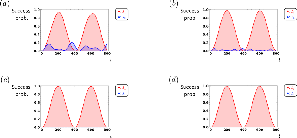
Figure 6: Success probabilities of our quantum algorithm. In this figure, we set $n=2^{16}$ and $m=2$. The two marked items in $\mathcal{X}_{1,0}$ and $\mathcal{X}_{1,\tilde{\epsilon}}$ are denoted as $\tilde{x}_{1}$ and $\tilde{x}_{2}$, respectively. The red and blue curves represent $P_{\rm suc}^{(\tilde{x}_{1})}(\vec{\epsilon},t)$ and $P_{\rm suc}^{(\tilde{x}_{2})}(\vec{\epsilon},t)$, respectively. (a) The case of $\tilde{\epsilon}=-0.01$. (b) The case of $\tilde{\epsilon}=-0.02$. (c) The case of $\tilde{\epsilon}=-0.05$. (d) The case of $\tilde{\epsilon}=-0.1$.

The above analysis enables us to perform the numerical simulation with $n=2^{16}$ that is quadratically larger than that in Figs. 2, 3, and 4. In Fig. 6, we plot $P_{\rm suc}^{(\tilde{x}_{1})}(\vec{\epsilon},t)$ and $P_{\rm suc}^{(\tilde{x}_{2})}(\vec{\epsilon},t)$ for several values of $\tilde{\epsilon}$. As $\tilde{\epsilon}$ decreases, the first local maxima of $P_{\rm suc}^{(\tilde{x}_{1})}(\vec{\epsilon},t)$ and $P_{\rm suc}^{(\tilde{x}_{2})}(\vec{\epsilon},t)$ tend to increase and decrease, respectively. In Appendix B, we analytically approximate $\sum_{x\in\mathcal{X}_{1,0}}P_{\rm suc}^{(x)}(\vec{\epsilon},t)$ and $\sum_{x\in\mathcal{X}_{1,\tilde{\epsilon}}}P_{\rm suc}^{(x)}(\vec{\epsilon},t)$. As a result, it turns out that these probabilities are $\sin^{2}{((2t+1)\theta/2)}/2+O(\tilde{\epsilon}^{2})$ when $t$ and $\theta$ are fixed [for details, see Eqs. (85) and (89)]. The original Grover’s algorithm is quite robust against the correlated phase errors in the sense that the probabilities do not linearly depend on the noise strength $|\tilde{\epsilon}|$. Furthermore, in Appendix B, we analytically show that when $|\tilde{\epsilon}|$ is sufficiently small but not $0$, the inequality $\sum_{x\in\mathcal{X}_{1,0}}P_{\rm suc}^{(x)}(\vec{\epsilon},t)>\sum_{x\in\mathcal{X}_{1,\tilde{\epsilon}}}P_{\rm suc}^{(x)}(\vec{\epsilon},t)$ holds by setting $t$ so that (i) $0\leq t\theta\ ({\rm mod}\ 2\pi)\leq\pi/2$ and (ii) $t>1/\tan{(\theta)}$. This sufficient condition is consistent with the fact that $P_{\rm suc}^{(\tilde{x}_{1})}(\vec{\epsilon},\lfloor\pi/(2\theta)\rfloor)>P_{\rm suc}^{(\tilde{x}_{2})}(\vec{\epsilon},\lfloor\pi/(2\theta)\rfloor)$ holds in Fig. 2.

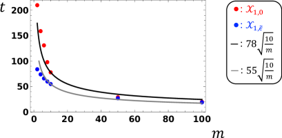
Figure 7: The numbers $t$ of queries such that $\sum_{x\in\mathcal{X}_{1,0}}P_{\rm suc}^{(x)}(\vec{\epsilon},t)$ and $\sum_{x\in\mathcal{X}_{1,\tilde{\epsilon}}}P_{\rm suc}^{(x)}(\vec{\epsilon},t)$ take the first local maxima. In this figure, we set $n=2^{16}$ and $\tilde{\epsilon}=-0.01$. The red and blue dots correspond to $\mathcal{X}_{1,0}$ and $\mathcal{X}_{1,\tilde{\epsilon}}$, respectively. The black and gray curves represent $78\sqrt{10/m}$ and $55\sqrt{10/m}$, respectively.

In Fig. 7, we also investigate the dependence of the query complexity of our algorithm on the number $m$ of marked items. As with the original Grover’s algorithm, the query complexity decreases with increasing $m$ and seems to approximately behave as being proportional to $1/\sqrt{m}$ in the range of $2\leq m\leq 100$.

III.3 Effect of quantum coherence between marked items

In this section, we examine the effect of coherence between the marked items in the initial state $|\psi(0)\rangle$. To this end, we consider the same situation as Sec. III.2. More specifically, we assume $m=2$, and the two marked items $\tilde{x}_{1}$ and $\tilde{x}_{2}$ are in the sets $\mathcal{X}_{1,0}$ and $\mathcal{X}_{1,\tilde{\epsilon}}$, respectively. We further assume $n=1000$ for simplicity. In this case, the ideal initial state in Eq. (18) is

$$|\psi(0)\rangle=\sqrt{\cfrac{499}{500}}|0_{L}\rangle+\cfrac{1}{\sqrt{1000}}\left(|\tilde{x}_{1}\rangle+|\tilde{x}_{2}\rangle\right).$$ (33)

It is apparent that the state in Eq. (33) has the coherence between the first and second marked items. More formally, when this state is projected onto the space of $\{|\tilde{x}_{1}\rangle,|\tilde{x}_{2}\rangle\}$, it becomes $(|\tilde{x}_{1}\rangle+|\tilde{x}_{2}\rangle)/\sqrt{2}$. To quantify its coherence, we use the $l_{1}$-norm of coherence BCP14 . Let $c_{j,k}$ be the $(j,k)$ element of any density operator $\rho$, i.e., $\rho=\sum_{j,k\in\mathcal{X}}c_{j,k}|j\rangle\langle k|$. The $l_{1}$-norm of coherence is defined as

$$C_{l_{1}}\left(\rho\right)\equiv\sum_{j,k\in\mathcal{X}}|c_{j,k}|-\sum_{j\in\mathcal{X}}|c_{j,j}|.$$ (34)

By definition, we obtain

$$C_{l_{1}}\left(\cfrac{|\tilde{x}_{1}\rangle+|\tilde{x}_{2}\rangle}{\sqrt{2}}\cfrac{\langle\tilde{x}_{1}|+\langle\tilde{x}_{2}|}{\sqrt{2}}\right)=1,$$ (35)

which is non-zero, and hence $(|\tilde{x}_{1}\rangle+|\tilde{x}_{2}\rangle)/\sqrt{2}$ is a coherent state. We consider how the success probability and query complexity change if the initial state is replaced with the incoherent state

$$\rho_{0}\equiv\cfrac{1}{2}\left[\cfrac{1}{1000}\left(\sqrt{999}|0_{L}\rangle+|\tilde{x}_{1}\rangle\right)\left(\sqrt{999}\langle 0_{L}|+\langle\tilde{x}_{1}|\right)+\cfrac{1}{1000}\left(\sqrt{999}|0_{L}\rangle+|\tilde{x}_{2}\rangle\right)\left(\sqrt{999}\langle 0_{L}|+\langle\tilde{x}_{2}|\right)\right].$$ (36)

Note that $|0_{L}\rangle$ does not include $|\tilde{x}_{1}\rangle$ and $|\tilde{x}_{2}\rangle$ [see Eq. (5)]. Therefore, $|\tilde{x}_{1}\rangle$ and $|\tilde{x}_{2}\rangle$ are not included in the second and first terms, respectively, but they will be produced by Grover’s diffusion operator during the algorithm. When $\rho_{0}$ is projected onto the space of $\{|\tilde{x}_{1}\rangle,|\tilde{x}_{2}\rangle\}$, it becomes $(|\tilde{x}_{1}\rangle\langle\tilde{x}_{1}|+|\tilde{x}_{2}\rangle\langle\tilde{x}_{2}|)/2$, which is incoherent because

$$C_{l_{1}}\left(\cfrac{|\tilde{x}_{1}\rangle\langle\tilde{x}_{1}|+|\tilde{x}_{2}\rangle\langle\tilde{x}_{2}|}{2}\right)=0.$$ (37)

The reason of why we use $\rho_{0}$ as an incoherent state is given in Appendix C.

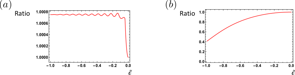
Figure 8: Ratios of the first local maximum of the success probability $P_{\rm suc}^{(x)}(\vec{\epsilon},t)$ with the ideal initial state $|\psi(0)\rangle$ to that with the incoherent initial state $\rho_{0}$. In this figure, we set $n=1000$ and $m=2$ and assume that the first and second marked items $\tilde{x}_{1}$ and $\tilde{x}_{2}$ are in the sets $\mathcal{X}_{1,0}$ and $\mathcal{X}_{1,\tilde{\epsilon}}$, respectively. (a) The case of $x=\tilde{x}_{1}$. That is, the ratio of the probability of finding the first marked item with $|\psi(0)\rangle$ to that with $\rho_{0}$. (b) The case of $x=\tilde{x}_{2}$.

Recall that $P_{\rm suc}^{(\tilde{x}_{i})}(\vec{\epsilon},t)$ is the probability of obtaining the $i$th marked item $\tilde{x}_{i}$ by measuring $[D\tilde{O}_{f}(\tilde{\epsilon})]^{t}|\psi(0)\rangle$ in the basis $\{|x\rangle\}_{x\in\mathcal{X}}$. Similarly, we define $H_{\rm suc}^{(\tilde{x}_{i})}(\vec{\epsilon},t)$ as the probability of obtaining $\tilde{x}_{i}$ by measuring $[D\tilde{O}_{f}(\tilde{\epsilon})]^{t}\rho_{0}[\tilde{O}_{f}^{\dagger}(\tilde{\epsilon})D^{\dagger}]^{t}$ in the same basis. For any $i$, let $P_{\rm opt}^{(\tilde{x}_{i})}(\tilde{\epsilon})$ and $H_{\rm opt}^{(\tilde{x}_{i})}(\tilde{\epsilon})$ be the first local maxima of $P_{\rm suc}^{(\tilde{x}_{i})}(\vec{\epsilon},t)$ and $H_{\rm suc}^{(\tilde{x}_{i})}(\vec{\epsilon},t)$ over $t$, respectively. In Fig. 8, we plot the ratios $P_{\rm opt}^{(\tilde{x}_{1})}(\tilde{\epsilon})/H_{\rm opt}^{(\tilde{x}_{1})}(\tilde{\epsilon})$ and $P_{\rm opt}^{(\tilde{x}_{2})}(\tilde{\epsilon})/H_{\rm opt}^{(\tilde{x}_{2})}(\tilde{\epsilon})$. Since the ratio in Fig. 8(a) is at least $1$, this figure would imply that the coherence between $\tilde{x}_{1}$ and $\tilde{x}_{2}$ increases the success probability of finding the first marked item $\tilde{x}_{1}$ in our quantum algorithm. On the other hand, the ratio in Fig. 8(b) is at most $1$, and hence the coherence has the opposite influence on the probability of finding the second marked item $\tilde{x}_{2}$.

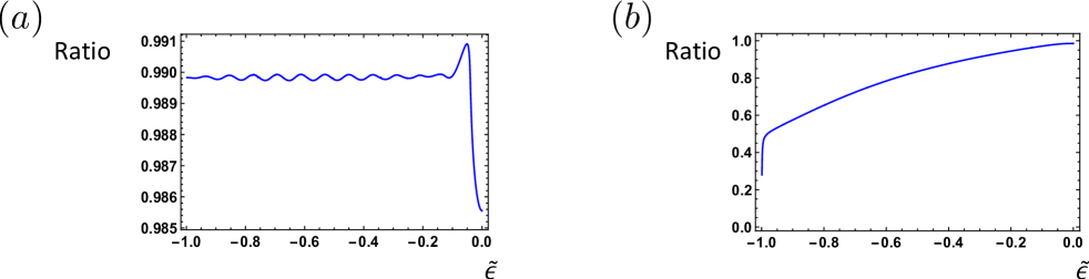
Figure 9: Ratios $t_{\rm opt}^{(|\psi(0)\rangle)}(x)/t_{\rm opt}^{(\rho_{0})}(x)$. In this figure, we set $n=1000$ and $m=2$ and assume that the first and second marked items $\tilde{x}_{1}$ and $\tilde{x}_{2}$ are in the sets $\mathcal{X}_{1,0}$ and $\mathcal{X}_{1,\tilde{\epsilon}}$, respectively. (a) The case of $x=\tilde{x}_{1}$. That is, the ratio of the smallest argument of the local maximum of the success probability of finding $\tilde{x}_{1}$ with the initial state $|\psi(0)\rangle$ to that with $\rho_{0}$. (b) The case of $x=\tilde{x}_{2}$.

We next consider the query complexity. For any $i$, let $t_{\rm opt}^{(|\psi(0)\rangle)}(\tilde{x}_{i})$ and $t_{\rm opt}^{(\rho_{0})}(\tilde{x}_{i})$ be the numbers of queries such that $P_{\rm suc}^{(\tilde{x}_{i})}(\vec{\epsilon},t_{\rm opt}^{(|\psi(0)\rangle)}(\tilde{x}_{i}))=P_{\rm opt}^{(\tilde{x}_{i})}(\tilde{\epsilon})$ and $H_{\rm suc}^{(\tilde{x}_{i})}(\vec{\epsilon},t_{\rm opt}^{(\rho_{0})}(\tilde{x}_{i}))=H_{\rm opt}^{(\tilde{x}_{i})}(\tilde{\epsilon})$, respectively. We numerically calculate the dependence of the ratios $t_{\rm opt}^{(|\psi(0)\rangle)}(\tilde{x}_{1})/t_{\rm opt}^{(\rho_{0})}(\tilde{x}_{1})$ and $t_{\rm opt}^{(|\psi(0)\rangle)}(\tilde{x}_{2})/t_{\rm opt}^{(\rho_{0})}(\tilde{x}_{2})$ on the priority parameter $\tilde{\epsilon}$ in Fig. 9. Unlike Fig. 8, the ratio of the query complexity is less than $1$ for all $\tilde{\epsilon}$ owing to the coherence between the two marked items in both cases of $i=1$ and $2$. This phenomenon would imply that the coherence accelerates our quantum algorithm.

The ratios in Figs. 8(a) and 9(a) sharply increase as $\tilde{\epsilon}$ decreases in the vicinity of $\tilde{\epsilon}=0$. These regions of $\tilde{\epsilon}$ almost overlap each other. Since $P_{\rm opt}^{(\tilde{x}_{1})}(\tilde{\epsilon})$ rapidly increases to almost $1$ in this region of Fig. 8(a), we qualitatively conclude that the rapid increase of $P_{\rm opt}^{(\tilde{x}_{1})}(\tilde{\epsilon})$ causes the faster increase of $t_{\rm opt}^{(|\psi(0)\rangle)}(\tilde{x}_{1})$ than that of $t_{\rm opt}^{(\rho_{0})}(\tilde{x}_{1})$, and hence we observe the sharp increase in Fig. 9(a).

III.4 Comparison with algorithm in Ref. PS08

In this section, we compare the performance of our quantum algorithm with that of the algorithm in Ref. PS08 . For simplicity, we concretely consider the same situation as Sec. III.2 with $n=8$ and $m=2$. In this case, the algorithm in Ref. PS08 uses the oracle operator

$$O_{f}^{({\rm PS})}(\epsilon)\equiv I^{(8)}-2\left(\sqrt{1+\epsilon}|\tilde{x}_{1}\rangle+\sqrt{-\epsilon}|\tilde{x}_{2}\rangle\right)\left(\sqrt{1+\epsilon}\langle\tilde{x}_{1}|+\sqrt{-\epsilon}\langle\tilde{x}_{2}|\right)$$ (38)

with $-1\leq\epsilon\leq 0$, and thus its final state is $[DO_{f}^{({\rm PS})}(\epsilon)]^{t}|\psi(0)\rangle$. The query complexity $t$ of this algorithm is the closet integer to

$$\cfrac{\cos^{-1}{\left(\sqrt{\cfrac{1+\epsilon}{n}}+\sqrt{-\cfrac{\epsilon}{n}}\right)}}{2\sin^{-1}{\left(\sqrt{\cfrac{1+\epsilon}{n}}+\sqrt{-\cfrac{\epsilon}{n}}\right)}}.$$ (39)

Therefore, when $n=8$, we can numerically show $t=1$ in the range of $-0.99\leq\epsilon\leq-0.01$. As a result, the final state becomes

$$DO_{f}^{({\rm PS})}(\epsilon)|\psi(0)\rangle=\left(\cfrac{1}{2}-\sqrt{-\epsilon(1+\epsilon)}\right)|\psi(0)\rangle+\left(\sqrt{\cfrac{1+\epsilon}{2}}+\sqrt{-\cfrac{\epsilon}{2}}\right)\left(\sqrt{1+\epsilon}|\tilde{x}_{1}\rangle+\sqrt{-\epsilon}|\tilde{x}_{2}\rangle\right).$$ (40)

By direct calculation, the probabilities $Q_{\rm suc}^{(\tilde{x}_{1})}(\epsilon)$ and $Q_{\rm suc}^{(\tilde{x}_{2})}(\epsilon)$ of the algorithm in Ref. PS08 finding the marked items $\tilde{x}_{1}$ and $\tilde{x}_{2}$ are

$$Q_{\rm suc}^{(\tilde{x}_{1})}(\epsilon)=\cfrac{\left[1+2\sqrt{-\epsilon(1+\epsilon)}+4(1+\epsilon)\right]^{2}}{32}$$ (41)

and

$$Q_{\rm suc}^{(\tilde{x}_{2})}(\epsilon)=\cfrac{\left[1+2\sqrt{-\epsilon(1+\epsilon)}-4\epsilon\right]^{2}}{32},$$ (42)

respectively.

On the other hand, under the same condition, our oracle operator in Eq. (15) becomes

$$\tilde{O}_{f}(\tilde{\epsilon})=I^{(8)}-2|\tilde{x}_{1}\rangle\langle\tilde{x}_{1}|-(1+e^{i\pi\tilde{\epsilon}})|\tilde{x}_{2}\rangle\langle\tilde{x}_{2}|.$$ (43)

By setting $t=2$, the final state of our algorithm becomes

$$\left[D\tilde{O}_{f}(\tilde{\epsilon})\right]^{2}|\psi(0)\rangle=-\cfrac{7+6e^{i\pi\tilde{\epsilon}}+3e^{2i\pi\tilde{\epsilon}}}{16}|\psi(0)\rangle+\cfrac{5-e^{i\pi\tilde{\epsilon}}}{4\sqrt{2}}|\tilde{x}_{1}\rangle+\cfrac{\left(1+e^{i\pi\tilde{\epsilon}}\right)\left(1+3e^{i\pi\tilde{\epsilon}}\right)}{8\sqrt{2}}|\tilde{x}_{2}\rangle.$$ (44)

Here, we define $P_{\rm suc}^{(\tilde{x}_{j})}(\tilde{\epsilon})\equiv P_{\rm suc}^{(\tilde{x}_{j})}(\vec{\epsilon},2)$ for all $1\leq j\leq 2$. The probabilities $P_{\rm suc}^{(\tilde{x}_{1})}(\tilde{\epsilon})$ and $P_{\rm suc}^{(\tilde{x}_{2})}(\tilde{\epsilon})$ of our algorithm finding the marked items $\tilde{x}_{1}$ and $\tilde{x}_{2}$ are

$$P_{\rm suc}^{(\tilde{x}_{1})}(\tilde{\epsilon})=\cfrac{373-210\cos{(\tilde{\epsilon}\pi)}-99\cos^{2}{(\tilde{\epsilon}\pi)}}{512}$$ (45)

and

$$P_{\rm suc}^{(\tilde{x}_{2})}(\tilde{\epsilon})=\cfrac{61+30\cos{(\tilde{\epsilon}\pi)}-27\cos^{2}{(\tilde{\epsilon}\pi)}}{512},$$ (46)

respectively.

To compare the two algorithms, we calculate the overall success probabilities $Q_{\rm suc}(\epsilon)\equiv Q_{\rm suc}^{(\tilde{x}_{1})}(\epsilon)+Q_{\rm suc}^{(\tilde{x}_{2})}(\epsilon)$ and $P_{\rm suc}(\tilde{\epsilon})\equiv P_{\rm suc}^{(\tilde{x}_{1})}(\tilde{\epsilon})+P_{\rm suc}^{(\tilde{x}_{2})}(\tilde{\epsilon})$ under the following conditions:

1. $-0.99\leq\epsilon\leq-0.01$

2. $-0.99\leq\tilde{\epsilon}\leq-0.01$

3. $Q_{\rm suc}^{(\tilde{x}_{1})}(\epsilon)/Q_{\rm suc}^{(\tilde{x}_{2})}(\epsilon)=P_{\rm suc}^{(\tilde{x}_{1})}(\tilde{\epsilon})/P_{\rm suc}^{(\tilde{x}_{2})}(\tilde{\epsilon})=R$ for a fixed real value $R$.

When $R=16.81$, $\epsilon=(62\sqrt{679}-1879)/22730$ and $\tilde{\epsilon}=\cos^{-1}{((11905-4\sqrt{24935893})/11829)}/\pi$ hold, and thus $Q_{\rm suc}((62\sqrt{679}-1879)/22730)\simeq 0.885$ and $P_{\rm suc}(\cos^{-1}{((11905-4\sqrt{24935893})/11829)}/\pi)\simeq 0.972$. On the other hand, when $R=4$, $\epsilon=(2\sqrt{7}-19)/74$ and $\tilde{\epsilon}=\cos^{-1}{((55-4\sqrt{181})/3)}/\pi$ hold, and thus $Q_{\rm suc}((2\sqrt{7}-19)/74)\simeq 0.991$ and $P_{\rm suc}(\cos^{-1}{((55-4\sqrt{181})/3)}/\pi)\simeq 0.67$. In short, when $R=16.81$ and $R=4$, our algorithm is superior and inferior to the algorithm in Ref. PS08 , respectively. From these observations, we can anticipate that when we would like to achieve a high ratio $R$, our algorithm would be preferred, but when $R$ is sufficiently low, the existing algorithm is preferable. It would be indispensable for a more detailed comparison to clarify how efficiently these two types of oracle operators can be constructed. Although the clarification is beyond the scope of this paper, the construction of our oracle operator was explored in Ref. SBCJKMMPBS24 .

IV Conclusion & Discussion

We have generalized Grover’s algorithm so that it finds multiple marked items with probabilities according to their priority. Our quantum algorithm can also be considered as the original Grover’s algorithm with correlated phase errors. We have elaborately analyzed the case where there are two kinds of priority parameters $0$ and $-1\leq\tilde{\epsilon}\leq 0$. We have finally compared our quantum algorithm with the existing algorithm PS08 and have concluded that which algorithm performs better depends on the priority parameters.

As an outlook, it would be interesting to analyze our quantum algorithm even in the case where more than two kinds of priority parameters. When there are $k$ kinds of priority parameters, our analytical approach in Sec. III.2 requires to solve a $(k+1)$th-degree equation. Since it is, in general, hard to solve equations with more than fourth degree, the more thorough analysis may necessitate a different approach.

In the original Grover’s algorithm, if the number $t$ of queries exceeds the optimal value in Eq. (11), the success probability tragically decreases. In this sense, the original algorithm needs to know the number $m$ of marked items. This issue was affirmatively solved by generalizing Grover’s algorithm so that it works even if the exact value of $m$ is unknown BBHT99 ; YLC14 ; CBD23 . It is open whether the same generalization can be achieved for our quantum algorithm.

Recently, several quantum algorithms, which include a quantum algorithm for unstructured search, were understood in a unified way by using the quantum singular value transformation (QSVT) MRTC21 . It would also be interesting to try to understand our quantum algorithm in the framework of the QSVT.

Although we consider only the noise on the oracle operator, other noise models such as the random Gaussian noise on quantum states PR99 , the unitary noise on the Hadamard gate SMB03 , and the coherent phase noise on (the generalized) Grover’s diffusion operator LYW23 were also investigated. To understand the noise robustness of the original Grover’s algorithm more deeply, it would be effective to combine our noise model with them.

DATA AVAILABILITY STATEMENT

The data that support the findings of this study are available upon reasonable request to the authors.

Appendix A DERIVATION OF EQS. (23) AND (25)

Let $|\phi\rangle=\alpha|0_{L}\rangle+\beta|1^{\prime}_{L}\rangle+\gamma|1^{\prime\prime}_{L}\rangle$ be a normalized eigenvector of $D\tilde{O}_{f}(\tilde{\epsilon})$ associated with the eigenvalue $\lambda$. Since we can assume that $\gamma$ is real without loss of generality, $|\alpha|^{2}+|\beta|^{2}+\gamma^{2}=1$. From $D\tilde{O}_{f}(\tilde{\epsilon})|\phi\rangle=\lambda|\phi\rangle$, we obtain the following system of equations:

$$\left\{\begin{array}[]{lll}\left[\cos{\left(\theta\right)}-\lambda\right]\alpha-\cfrac{\sin{\left(\theta\right)}}{\sqrt{2}}\beta-e^{i\pi\tilde{\epsilon}}\cfrac{\sin{\left(\theta\right)}}{\sqrt{2}}\gamma&=&0\\ \cfrac{\sin{\left(\theta\right)}}{\sqrt{2}}\alpha+\left[\cfrac{1+\cos{\left(\theta\right)}}{2}-\lambda\right]\beta-e^{i\pi\tilde{\epsilon}}\cfrac{1-\cos{\left(\theta\right)}}{2}\gamma&=&0\\ \cfrac{\sin{\left(\theta\right)}}{\sqrt{2}}\alpha-\cfrac{1-\cos{\left(\theta\right)}}{2}\beta+\left[e^{i\pi\tilde{\epsilon}}\cfrac{1+\cos{\left(\theta\right)}}{2}-\lambda\right]\gamma&=&0.\end{array}\right.$$ (50)

Since $D\tilde{O}_{f}(\tilde{\epsilon})$ is a unitary operator, $|\lambda|=1$. On the other hand, from $1\leq m\leq n/2$, we have $0\leq\cos{\left(\theta\right)}<1$ because $\cos{\left(\theta\right)}=1-2\sin^{2}{\left(\theta/2\right)}=1-2m/n$. Therefore, $\lambda\neq\cos{\left(\theta\right)}$, and hence the first equality in Eq. (50) implies

$$\alpha=\cfrac{\sin{\left(\theta\right)}\left(\beta+e^{i\pi\tilde{\epsilon}}\gamma\right)}{\sqrt{2}\left[\cos{\left(\theta\right)}-\lambda\right]}.$$ (51)

By substituting Eq. (51) into the second equality in Eq. (50),

$$\cfrac{\sin{\left(\theta\right)}}{\sqrt{2}}\cfrac{\sin{\left(\theta\right)}\left(\beta+e^{i\pi\tilde{\epsilon}}\gamma\right)}{\sqrt{2}\left[\cos{\left(\theta\right)}-\lambda\right]}+\left[\cfrac{1+\cos{\left(\theta\right)}}{2}-\lambda\right]\beta-e^{i\pi\tilde{\epsilon}}\cfrac{1-\cos{\left(\theta\right)}}{2}\gamma=0$$ (52)

$$\Rightarrow \cfrac{\sin^{2}{\left(\theta\right)}+\left[1+\cos{\left(\theta\right)}-2\lambda\right]\left[\cos{\left(\theta\right)}-\lambda\right]}{2\left[\cos{\left(\theta\right)}-\lambda\right]}\beta+e^{i\pi\tilde{\epsilon}}\cfrac{\sin^{2}{\left(\theta\right)}-\left[1-\cos{\left(\theta\right)}\right]\left[\cos{\left(\theta\right)}-\lambda\right]}{2\left[\cos{\left(\theta\right)}-\lambda\right]}\gamma=0$$ (53)

$$\Rightarrow \cfrac{\left(1-\lambda\right)\left[1+\cos{\left(\theta\right)}\right]+2\lambda\left[\lambda-\cos{\left(\theta\right)}\right]}{2\left[\cos{\left(\theta\right)}-\lambda\right]}\beta+e^{i\pi\tilde{\epsilon}}\cfrac{\left(1+\lambda\right)\left[1-\cos{\left(\theta\right)}\right]}{2\left[\cos{\left(\theta\right)}-\lambda\right]}\gamma=0.$$ (54)

To prove that the coefficient of $\beta$ in Eq. (54) is not $0$, we show $\left(1-\lambda\right)\left[1+\cos{\left(\theta\right)}\right]+2\lambda\left[\lambda-\cos{\left(\theta\right)}\right]\neq 0$ for any $\lambda$ and $\theta$ under the condition $0\leq\cos{\left(\theta\right)}<1$. If $\left(1-\lambda\right)\left[1+\cos{\left(\theta\right)}\right]+2\lambda\left[\lambda-\cos{\left(\theta\right)}\right]=0$, then

$$\lambda=\cfrac{1+3\cos{\left(\theta\right)}\pm\sqrt{\left[1+3\cos{\left(\theta\right)}\right]^{2}-8\left[1+\cos{\left(\theta\right)}\right]}}{4}=\cfrac{1+3\cos{\left(\theta\right)}\pm i\sqrt{\left[1-\cos{\left(\theta\right)}\right]\left[7+9\cos{\left(\theta\right)}\right]}}{4}$$ (55)

$$\Rightarrow |\lambda|^{2}=\cfrac{\left[1+3\cos{\left(\theta\right)}\right]^{2}+\left[1-\cos{\left(\theta\right)}\right]\left[7+9\cos{\left(\theta\right)}\right]}{16}=\cfrac{1+\cos{\left(\theta\right)}}{2}.$$ (56)

Therefore, $|\lambda|\neq 1$, which contradicts to the fact that $D\tilde{O}_{f}(\tilde{\epsilon})$ is a unitary operator. In conclusion, $\left(1-\lambda\right)\left[1+\cos{\left(\theta\right)}\right]+2\lambda\left[\lambda-\cos{\left(\theta\right)}\right]\neq 0$. Now, we can immediately obtain

$$\beta=-e^{i\pi\tilde{\epsilon}}\cfrac{(1+\lambda)\left[1-\cos{\left(\theta\right)}\right]}{(1-\lambda)\left[1+\cos{\left(\theta\right)}\right]+2\lambda\left[\lambda-\cos{\left(\theta\right)}\right]}\gamma$$ (57)

from Eq. (54). By substituting Eq. (57) into Eq. (51),

$$\alpha = \cfrac{\sin{\left(\theta\right)}}{\sqrt{2}\left[\cos{\left(\theta\right)}-\lambda\right]}\left\{-e^{i\pi\tilde{\epsilon}}\cfrac{(1+\lambda)\left[1-\cos{\left(\theta\right)}\right]}{(1-\lambda)\left[1+\cos{\left(\theta\right)}\right]+2\lambda\left[\lambda-\cos{\left(\theta\right)}\right]}+e^{i\pi\tilde{\epsilon}}\right\}\gamma$$ (58)

$$= e^{i\pi\tilde{\epsilon}}\cfrac{\sqrt{2}(1-\lambda)\sin{\left(\theta\right)}}{(1-\lambda)\left[1+\cos{\left(\theta\right)}\right]+2\lambda\left[\lambda-\cos{\left(\theta\right)}\right]}\gamma.$$ (59)

By using Eqs. (57) and (59),

$$|\alpha|^{2}+|\beta|^{2}+\gamma^{2}=1$$ (60)

$$\Rightarrow \cfrac{2|1-\lambda|^{2}\sin^{2}{\left(\theta\right)}}{|(1-\lambda)\left[1+\cos{\left(\theta\right)}\right]+2\lambda\left[\lambda-\cos{\left(\theta\right)}\right]|^{2}}\gamma^{2}+\cfrac{|1+\lambda|^{2}\left[1-\cos{\left(\theta\right)}\right]^{2}}{|(1-\lambda)\left[1+\cos{\left(\theta\right)}\right]+2\lambda\left[\lambda-\cos{\left(\theta\right)}\right]|^{2}}\gamma^{2}+\gamma^{2}=1$$ (61)

$$\Rightarrow \gamma=\cfrac{|(1-\lambda)\left[1+\cos{\left(\theta\right)}\right]+2\lambda\left[\lambda-\cos{\left(\theta\right)}\right]|}{\sqrt{2|1-\lambda|^{2}\sin^{2}{\left(\theta\right)}+|1+\lambda|^{2}\left[1-\cos{\left(\theta\right)}\right]^{2}+|(1-\lambda)\left[1+\cos{\left(\theta\right)}\right]+2\lambda\left[\lambda-\cos{\left(\theta\right)}\right]|^{2}}}$$ (62)

$$\Rightarrow \gamma=\cfrac{|1+\cos{\left(\theta\right)}-\lambda\left[1+3\cos{\left(\theta\right)}-2\lambda\right]|}{\sqrt{2|1-\lambda|^{2}\sin^{2}{\left(\theta\right)}+|1+\lambda|^{2}\left[1-\cos{\left(\theta\right)}\right]^{2}+|1+\cos{\left(\theta\right)}-\lambda\left[1+3\cos{\left(\theta\right)}-2\lambda\right]|^{2}}}.$$ (63)

Eq. (63) together with Eqs. (57) and (59) implies our objective Eq. (23).

We next derive Eq. (25). It is obtained from the characteristic equation

$${\rm det}\left(D\tilde{O}_{f}(\tilde{\epsilon})-\lambda I^{(3)}\right)=0.$$ (64)

The left-hand side of Eq. (64) is

$$\left[\cos{\left(\theta\right)}-\lambda\right]\left[\cfrac{1+\cos{\left(\theta\right)}}{2}-\lambda\right]\left[e^{i\pi\tilde{\epsilon}}\cfrac{1+\cos{\left(\theta\right)}}{2}-\lambda\right]+e^{i\pi\tilde{\epsilon}}\sin^{2}{\left(\theta\right)}\cfrac{1-\cos{\left(\theta\right)}}{2}+e^{i\pi\tilde{\epsilon}}\cfrac{\sin^{2}{\left(\theta\right)}}{2}\left[\cfrac{1+\cos{\left(\theta\right)}}{2}-\lambda\right]$$ (68)

$$+\cfrac{\sin^{2}{\left(\theta\right)}}{2}\left[e^{i\pi\tilde{\epsilon}}\cfrac{1+\cos{\left(\theta\right)}}{2}-\lambda\right]-e^{i\pi\tilde{\epsilon}}\left[\cfrac{1-\cos{\left(\theta\right)}}{2}\right]^{2}\left[\cos{\left(\theta\right)}-\lambda\right]$$

$$= \left[\lambda^{2}-\cfrac{1+3\cos{\left(\theta\right)}}{2}\lambda+\cos{\left(\theta\right)}\cfrac{1+\cos{\left(\theta\right)}}{2}\right]\left[e^{i\pi\tilde{\epsilon}}\cfrac{1+\cos{\left(\theta\right)}}{2}-\lambda\right]+e^{i\pi\tilde{\epsilon}}\sin^{2}{\left(\theta\right)}\cfrac{1-\cos{\left(\theta\right)}}{2}+e^{i\pi\tilde{\epsilon}}\sin^{2}{\left(\theta\right)}\cfrac{1+\cos{\left(\theta\right)}}{2}$$

$$-e^{i\pi\tilde{\epsilon}}\cfrac{\sin^{2}{\left(\theta\right)}}{2}\lambda-\cfrac{\sin^{2}{\left(\theta\right)}}{2}\lambda-e^{i\pi\tilde{\epsilon}}\left[\cfrac{1-\cos{\left(\theta\right)}}{2}\right]^{2}\cos{\left(\theta\right)}+e^{i\pi\tilde{\epsilon}}\left[\cfrac{1-\cos{\left(\theta\right)}}{2}\right]^{2}\lambda$$

$$= -\lambda^{3}+\left[\cfrac{1+3\cos{\left(\theta\right)}}{2}+e^{i\pi\tilde{\epsilon}}\cfrac{1+\cos{\left(\theta\right)}}{2}\right]\lambda^{2}-\left[\cos{\left(\theta\right)}\cfrac{1+\cos{\left(\theta\right)}}{2}+e^{i\pi\tilde{\epsilon}}\cfrac{1+3\cos{\left(\theta\right)}}{2}\cfrac{1+\cos{\left(\theta\right)}}{2}\right]\lambda$$

$$+e^{i\pi\tilde{\epsilon}}\cos{\left(\theta\right)}\left[\cfrac{1+\cos{\left(\theta\right)}}{2}\right]^{2}+e^{i\pi\tilde{\epsilon}}\sin^{2}{\left(\theta\right)}-\left(1+e^{i\pi\tilde{\epsilon}}\right)\cfrac{\sin^{2}{\left(\theta\right)}}{2}\lambda-e^{i\pi\tilde{\epsilon}}\left[\cfrac{1-\cos{\left(\theta\right)}}{2}\right]^{2}\cos{\left(\theta\right)}+e^{i\pi\tilde{\epsilon}}\left[\cfrac{1-\cos{\left(\theta\right)}}{2}\right]^{2}\lambda$$

$$= -\lambda^{3}+\left[\cfrac{1+3\cos{\left(\theta\right)}}{2}+e^{i\pi\tilde{\epsilon}}\cfrac{1+\cos{\left(\theta\right)}}{2}\right]\lambda^{2}$$

$$-\left\{\cos{\left(\theta\right)}\cfrac{1+\cos{\left(\theta\right)}}{2}+e^{i\pi\tilde{\epsilon}}\left[\cfrac{3\cos^{2}{\left(\theta\right)}+4\cos{\left(\theta\right)}+1}{4}-\cfrac{\cos^{2}{\left(\theta\right)}-2\cos{\left(\theta\right)}+1}{4}\right]\right\}\lambda$$

$$+e^{i\pi\tilde{\epsilon}}\cos{\left(\theta\right)}\left[\cfrac{\cos^{2}{\left(\theta\right)}+2\cos{\left(\theta\right)}+1}{4}-\cfrac{\cos^{2}{\left(\theta\right)}-2\cos{\left(\theta\right)}+1}{4}\right]+e^{i\pi\tilde{\epsilon}}\sin^{2}{\left(\theta\right)}-\left(1+e^{i\pi\tilde{\epsilon}}\right)\cfrac{\sin^{2}{\left(\theta\right)}}{2}\lambda$$

$$= -\lambda^{3}+\left[\cfrac{1+3\cos{\left(\theta\right)}}{2}+e^{i\pi\tilde{\epsilon}}\cfrac{1+\cos{\left(\theta\right)}}{2}\right]\lambda^{2}-\left[\cfrac{\cos^{2}{\left(\theta\right)}+\cos{\left(\theta\right)}}{2}+\cfrac{\sin^{2}{\left(\theta\right)}}{2}+e^{i\pi\tilde{\epsilon}}\cfrac{1+3\cos{\left(\theta\right)}}{2}\right]\lambda+e^{i\pi\tilde{\epsilon}}$$ (69)

$$= -\lambda^{3}+\left[\cfrac{1+3\cos{\left(\theta\right)}}{2}+e^{i\pi\tilde{\epsilon}}\cfrac{1+\cos{\left(\theta\right)}}{2}\right]\lambda^{2}-\left[\cfrac{1+\cos{\left(\theta\right)}}{2}+e^{i\pi\tilde{\epsilon}}\cfrac{1+3\cos{\left(\theta\right)}}{2}\right]\lambda+e^{i\pi\tilde{\epsilon}}$$ (70)

$$= -\lambda^{3}+a(\theta,\tilde{\epsilon})\lambda^{2}-e^{i\pi\tilde{\epsilon}}a^{\ast}(\theta,\tilde{\epsilon})\lambda+e^{i\pi\tilde{\epsilon}},$$ (71)

where $a(\theta,\tilde{\epsilon})$ is defined in Eq. (26). By substituting Eq. (71) into Eq. (64), we immediately obtain Eq. (25).

Appendix B APPROXIMATION OF SUCCESS PROBABILITIES OF OUR ALGORITHM

Under the same situation as Sec. III.2 with $1\leq m\leq n/2$, we derive the approximation of the success probabilities $\sum_{x\in\mathcal{X}_{1,0}}P_{\rm suc}^{(x)}(\vec{\epsilon},t)$ and $\sum_{x\in\mathcal{X}_{1,\tilde{\epsilon}}}P_{\rm suc}^{(x)}(\vec{\epsilon},t)$ of our quantum algorithm. To this end, we transform the orthonormal basis from $\{|0_{L}\rangle,|1^{\prime}_{L}\rangle,|1^{\prime\prime}_{L}\rangle\}$ to $\{|0_{L}\rangle,|+_{L}\rangle,|-_{L}\rangle\}$ with $|\pm_{L}\rangle\equiv(|1^{\prime}_{L}\rangle\pm|1^{\prime\prime}_{L}\rangle)/\sqrt{2}$. From Eq. (22), the matrix form of $D\tilde{O}_{f}(\tilde{\epsilon})$ in this transformed basis is

$$\begin{pmatrix}\cos{\left(\theta\right)}&-\cfrac{1+e^{i\pi\tilde{\epsilon}}}{2}\sin{\left(\theta\right)}&-\cfrac{1-e^{i\pi\tilde{\epsilon}}}{2}\sin{\left(\theta\right)}\\ \sin{\left(\theta\right)}&\cfrac{1+e^{i\pi\tilde{\epsilon}}}{2}\cos{\left(\theta\right)}&\cfrac{1-e^{i\pi\tilde{\epsilon}}}{2}\cos{\left(\theta\right)}\\ 0&\cfrac{1-e^{i\pi\tilde{\epsilon}}}{2}&\cfrac{1+e^{i\pi\tilde{\epsilon}}}{2}\\ \end{pmatrix}=\begin{pmatrix}\cos{\left(\theta\right)}&-\sin{\left(\theta\right)}&0\\ \sin{\left(\theta\right)}&\cos{\left(\theta\right)}&0\\ 0&0&1\\ \end{pmatrix}+\cfrac{1-e^{i\pi\tilde{\epsilon}}}{2}\begin{pmatrix}0&\sin{\left(\theta\right)}&-\sin{\left(\theta\right)}\\ 0&-\cos{\left(\theta\right)}&\cos{\left(\theta\right)}\\ 0&1&-1\\ \end{pmatrix}.$$ (72)

Let

$$G\equiv\begin{pmatrix}\cos{\left(\theta\right)}&-\sin{\left(\theta\right)}&0\\ \sin{\left(\theta\right)}&\cos{\left(\theta\right)}&0\\ 0&0&1\\ \end{pmatrix}$$ (73)

and

$$E\equiv\begin{pmatrix}0&\sin{\left(\theta\right)}&-\sin{\left(\theta\right)}\\ 0&-\cos{\left(\theta\right)}&\cos{\left(\theta\right)}\\ 0&1&-1\\ \end{pmatrix}.$$ (74)

When $|\tilde{\epsilon}|$ is sufficiently small, $(1-e^{i\pi\tilde{\epsilon}})/2\simeq-i\pi\tilde{\epsilon}/2+\pi^{2}\tilde{\epsilon}^{2}/4$, and hence

$$\left[D\tilde{O}_{f}(\tilde{\epsilon})\right]^{t}\simeq G^{t}+\left(-i\cfrac{\pi}{2}\tilde{\epsilon}+\cfrac{\pi^{2}}{4}\tilde{\epsilon}^{2}\right)\sum_{j=0}^{t-1}G^{j}EG^{t-j-1}-\cfrac{\pi^{2}}{4}\tilde{\epsilon}^{2}\sum_{j=0}^{t-2}\sum_{k=0}^{t-j-2}G^{j}EG^{k}EG^{t-j-k-2}.$$ (75)

Note that in Eq. (75), when $t<2$, the third term is zero, and when $t=0$, the second term is also zero.

To achieve our purpose, it is sufficient to calculate $|\langle 1^{\prime}_{L}|[D\tilde{O}_{f}(\tilde{\epsilon})]^{t}|\psi(0)\rangle|^{2}$ and $|\langle 1^{\prime\prime}_{L}|[D\tilde{O}_{f}(\tilde{\epsilon})]^{t}|\psi(0)\rangle|^{2}$. To this end, we first derive the matrix form of $G^{l}E$ and calculate $G^{l}|\psi(0)\rangle$ for any $0\leq l\leq t$. Since $G$ is a rotation matrix, we obtain

$$G^{l}E=\begin{pmatrix}\cos{\left(l\theta\right)}&-\sin{\left(l\theta\right)}&0\\ \sin{\left(l\theta\right)}&\cos{\left(l\theta\right)}&0\\ 0&0&1\\ \end{pmatrix}\begin{pmatrix}0&\sin{\left(\theta\right)}&-\sin{\left(\theta\right)}\\ 0&-\cos{\left(\theta\right)}&\cos{\left(\theta\right)}\\ 0&1&-1\\ \end{pmatrix}=\begin{pmatrix}0&\sin{\left(\left(l+1\right)\theta\right)}&-\sin{\left(\left(l+1\right)\theta\right)}\\ 0&-\cos{\left(\left(l+1\right)\theta\right)}&\cos{\left(\left(l+1\right)\theta\right)}\\ 0&1&-1\\ \end{pmatrix}$$ (76)

and

$$G^{l}|\psi(0)\rangle=\begin{pmatrix}\cos{\left(l\theta\right)}&-\sin{\left(l\theta\right)}&0\\ \sin{\left(l\theta\right)}&\cos{\left(l\theta\right)}&0\\ 0&0&1\\ \end{pmatrix}\begin{pmatrix}\cos{\left(\cfrac{\theta}{2}\right)}\\ \sin{\left(\cfrac{\theta}{2}\right)}\\ 0\\ \end{pmatrix}=\begin{pmatrix}\cos{\left(\left(l+\cfrac{1}{2}\right)\theta\right)}\\ \sin{\left(\left(l+\cfrac{1}{2}\right)\theta\right)}\\ 0\\ \end{pmatrix}.$$ (77)

From Eqs. (75), (76), and (77),

$$\langle 1^{\prime}_{L}|[D\tilde{O}_{f}(\tilde{\epsilon})]^{t}|\psi(0)\rangle$$ (79)

$$\simeq \cfrac{1}{\sqrt{2}}\begin{pmatrix}0&1&1\\ \end{pmatrix}\left[\begin{pmatrix}\cos{\left(\left(t+\cfrac{1}{2}\right)\theta\right)}\\ \sin{\left(\left(t+\cfrac{1}{2}\right)\theta\right)}\\ 0\\ \end{pmatrix}\right.$$

$$+\left(-i\cfrac{\pi}{2}\tilde{\epsilon}+\cfrac{\pi^{2}}{4}\tilde{\epsilon}^{2}\right)\sum_{j=0}^{t-1}\begin{pmatrix}0&\sin{\left(\left(j+1\right)\theta\right)}&-\sin{\left(\left(j+1\right)\theta\right)}\\ 0&-\cos{\left(\left(j+1\right)\theta\right)}&\cos{\left(\left(j+1\right)\theta\right)}\\ 0&1&-1\\ \end{pmatrix}\begin{pmatrix}\cos{\left(\left(t-j-\cfrac{1}{2}\right)\theta\right)}\\ \sin{\left(\left(t-j-\cfrac{1}{2}\right)\theta\right)}\\ 0\\ \end{pmatrix}$$

$$+\cfrac{\pi^{2}}{4}\tilde{\epsilon}^{2}\sum_{j=0}^{t-2}\sum_{k=0}^{t-j-2}\left[1+\cos{\left((k+1)\theta\right)}\right]\left.\begin{pmatrix}0&\sin{\left(\left(j+1\right)\theta\right)}&-\sin{\left(\left(j+1\right)\theta\right)}\\ 0&-\cos{\left(\left(j+1\right)\theta\right)}&\cos{\left(\left(j+1\right)\theta\right)}\\ 0&1&-1\\ \end{pmatrix}\begin{pmatrix}\cos{\left(\left(t-j-k-\cfrac{3}{2}\right)\theta\right)}\\ \sin{\left(\left(t-j-k-\cfrac{3}{2}\right)\theta\right)}\\ 0\\ \end{pmatrix}\right]\ \ \ \ \$$

$$= \cfrac{\sin{\left(\left(t+\cfrac{1}{2}\right)\theta\right)}}{\sqrt{2}}+\left(-i\cfrac{\pi}{2}\tilde{\epsilon}+\cfrac{\pi^{2}}{4}\tilde{\epsilon}^{2}\right)\sum_{j=0}^{t-1}\cfrac{1-\cos{\left(\left(j+1\right)\theta\right)}}{\sqrt{2}}\sin{\left(\left(t-j-\cfrac{1}{2}\right)\theta\right)}$$

$$+\cfrac{\pi^{2}}{4}\tilde{\epsilon}^{2}\sum_{j=0}^{t-2}\sum_{k=0}^{t-j-2}\left[1+\cos{\left(\left(k+1\right)\theta\right)}\right]\cfrac{1-\cos{\left(\left(j+1\right)\theta\right)}}{\sqrt{2}}\sin{\left(\left(t-j-k-\cfrac{3}{2}\right)\theta\right)}.$$

For simplicity, we define

$$s_{1} \equiv \sum_{j=0}^{t-1}\left[1-\cos{\left(\left(j+1\right)\theta\right)}\right]\sin{\left(\left(t-j-\cfrac{1}{2}\right)\theta\right)}$$ (80)

$$= \cfrac{\sin^{2}{\left(\cfrac{t\theta}{2}\right)}}{\sin{\left(\cfrac{\theta}{2}\right)}}-\cfrac{1}{2}\sum_{j=0}^{t-1}\left[\sin{\left(\left(t+\cfrac{1}{2}\right)\theta\right)}+\sin{\left(\left(t-2j-\cfrac{3}{2}\right)\theta\right)}\right]$$ (81)

$$= \cfrac{\sin^{2}{\left(\cfrac{t\theta}{2}\right)}}{\sin{\left(\cfrac{\theta}{2}\right)}}-\cfrac{t}{2}\sin{\left(\left(t+\cfrac{1}{2}\right)\theta\right)}+\cfrac{\sin{\left(t\theta\right)}\sin{\left(\cfrac{\theta}{2}\right)}}{2\sin{\left(\theta\right)}}$$ (82)

and

$$s_{2}\equiv\sum_{j=0}^{t-2}\sum_{k=0}^{t-j-2}\left[1+\cos{\left(\left(k+1\right)\theta\right)}\right]\left[1-\cos{\left(\left(j+1\right)\theta\right)}\right]\sin{\left(\left(t-j-k-\cfrac{3}{2}\right)\theta\right)}.$$ (83)

From Eq. (79),

$$\sum_{x\in\mathcal{X}_{1,0}}P_{\rm suc}^{(x)}(\vec{\epsilon},t)=\left|\langle 1^{\prime}_{L}|[D\tilde{O}_{f}(\tilde{\epsilon})]^{t}|\psi(0)\rangle\right|^{2} \simeq \cfrac{\left|\sin{\left(\left(t+\cfrac{1}{2}\right)\theta\right)}+\cfrac{\pi^{2}}{4}\left(s_{1}+s_{2}\right)\tilde{\epsilon}^{2}-i\cfrac{\pi}{2}s_{1}\tilde{\epsilon}\right|^{2}}{2}$$ (84)

$$\simeq \cfrac{\sin^{2}{\left(\left(t+\cfrac{1}{2}\right)\theta\right)}+\cfrac{\pi^{2}}{4}\left[2\left(s_{1}+s_{2}\right)\sin{\left(\left(t+\cfrac{1}{2}\right)\theta\right)}+s_{1}^{2}\right]\tilde{\epsilon}^{2}}{2}.\ \ \ \ \$$ (85)

In a similar manner,

$$\langle 1^{\prime\prime}_{L}|[D\tilde{O}_{f}(\tilde{\epsilon})]^{t}|\psi(0)\rangle$$ (87)

$$\simeq \cfrac{1}{\sqrt{2}}\begin{pmatrix}0&1&-1\\ \end{pmatrix}\left[\begin{pmatrix}\cos{\left(\left(t+\cfrac{1}{2}\right)\theta\right)}\\ \sin{\left(\left(t+\cfrac{1}{2}\right)\theta\right)}\\ 0\\ \end{pmatrix}\right.$$

$$+\left(-i\cfrac{\pi}{2}\tilde{\epsilon}+\cfrac{\pi^{2}}{4}\tilde{\epsilon}^{2}\right)\sum_{j=0}^{t-1}\begin{pmatrix}0&\sin{\left(\left(j+1\right)\theta\right)}&-\sin{\left(\left(j+1\right)\theta\right)}\\ 0&-\cos{\left(\left(j+1\right)\theta\right)}&\cos{\left(\left(j+1\right)\theta\right)}\\ 0&1&-1\\ \end{pmatrix}\begin{pmatrix}\cos{\left(\left(t-j-\cfrac{1}{2}\right)\theta\right)}\\ \sin{\left(\left(t-j-\cfrac{1}{2}\right)\theta\right)}\\ 0\\ \end{pmatrix}$$

$$+\cfrac{\pi^{2}}{4}\tilde{\epsilon}^{2}\sum_{j=0}^{t-2}\sum_{k=0}^{t-j-2}\left[1+\cos{\left((k+1)\theta\right)}\right]\left.\begin{pmatrix}0&\sin{\left(\left(j+1\right)\theta\right)}&-\sin{\left(\left(j+1\right)\theta\right)}\\ 0&-\cos{\left(\left(j+1\right)\theta\right)}&\cos{\left(\left(j+1\right)\theta\right)}\\ 0&1&-1\\ \end{pmatrix}\begin{pmatrix}\cos{\left(\left(t-j-k-\cfrac{3}{2}\right)\theta\right)}\\ \sin{\left(\left(t-j-k-\cfrac{3}{2}\right)\theta\right)}\\ 0\\ \end{pmatrix}\right]\ \ \ \ \$$

$$= \cfrac{\sin{\left(\left(t+\cfrac{1}{2}\right)\theta\right)}}{\sqrt{2}}-\left(-i\cfrac{\pi}{2}\tilde{\epsilon}+\cfrac{\pi^{2}}{4}\tilde{\epsilon}^{2}\right)\sum_{j=0}^{t-1}\cfrac{1+\cos{\left(\left(j+1\right)\theta\right)}}{\sqrt{2}}\sin{\left(\left(t-j-\cfrac{1}{2}\right)\theta\right)}$$

$$-\cfrac{\pi^{2}}{4}\tilde{\epsilon}^{2}\sum_{j=0}^{t-2}\sum_{k=0}^{t-j-2}\left[1+\cos{\left(\left(k+1\right)\theta\right)}\right]\cfrac{1+\cos{\left(\left(j+1\right)\theta\right)}}{\sqrt{2}}\sin{\left(\left(t-j-k-\cfrac{3}{2}\right)\theta\right)},$$

and thus

$$\sum_{x\in\mathcal{X}_{1,\tilde{\epsilon}}}P_{\rm suc}^{(x)}(\vec{\epsilon},t)=\left|\langle 1^{\prime\prime}_{L}|[D\tilde{O}_{f}(\tilde{\epsilon})]^{t}|\psi(0)\rangle\right|^{2} \simeq \cfrac{\left|\sin{\left(\left(t+\cfrac{1}{2}\right)\theta\right)}-\cfrac{\pi^{2}}{4}\left(s_{3}+s_{4}\right)\tilde{\epsilon}^{2}+i\cfrac{\pi}{2}s_{3}\tilde{\epsilon}\right|^{2}}{2}$$ (88)

$$\simeq \cfrac{\sin^{2}{\left(\left(t+\cfrac{1}{2}\right)\theta\right)}+\cfrac{\pi^{2}}{4}\left[-2\left(s_{3}+s_{4}\right)\sin{\left(\left(t+\cfrac{1}{2}\right)\theta\right)}+s_{3}^{2}\right]\tilde{\epsilon}^{2}}{2},\ \ \ \ \ \ \$$ (89)

where

$$s_{3}\equiv\sum_{j=0}^{t-1}\left[1+\cos{\left(\left(j+1\right)\theta\right)}\right]\sin{\left(\left(t-j-\cfrac{1}{2}\right)\theta\right)}=\cfrac{\sin^{2}{\left(\cfrac{t\theta}{2}\right)}}{\sin{\left(\cfrac{\theta}{2}\right)}}+\cfrac{t}{2}\sin{\left(\left(t+\cfrac{1}{2}\right)\theta\right)}-\cfrac{\sin{\left(t\theta\right)}\sin{\left(\cfrac{\theta}{2}\right)}}{2\sin{\left(\theta\right)}}$$ (90)

and

$$s_{4}\equiv\sum_{j=0}^{t-2}\sum_{k=0}^{t-j-2}\left[1+\cos{\left(\left(k+1\right)\theta\right)}\right]\left[1+\cos{\left(\left(j+1\right)\theta\right)}\right]\sin{\left(\left(t-j-k-\cfrac{3}{2}\right)\theta\right)}.$$ (91)

To evaluate how largely the marked items in $\mathcal{X}_{1,0}$ are prioritized than the other marked items in $\mathcal{X}_{1,\tilde{\epsilon}}$, it would be informative to calculate the gap $\sum_{x\in\mathcal{X}_{1,0}}P_{\rm suc}^{(x)}(\vec{\epsilon},t)-\sum_{x\in\mathcal{X}_{1,\tilde{\epsilon}}}P_{\rm suc}^{(x)}(\vec{\epsilon},t)$. From Eqs. (85) and (89),

$$\sum_{x\in\mathcal{X}_{1,0}}P_{\rm suc}^{(x)}(\vec{\epsilon},t)-\sum_{x\in\mathcal{X}_{1,\tilde{\epsilon}}}P_{\rm suc}^{(x)}(\vec{\epsilon},t)$$ (92)

$$= \left|\langle 1^{\prime}_{L}|[D\tilde{O}_{f}(\tilde{\epsilon})]^{t}|\psi(0)\rangle\right|^{2}-\left|\langle 1^{\prime\prime}_{L}|[D\tilde{O}_{f}(\tilde{\epsilon})]^{t}|\psi(0)\rangle\right|^{2}$$

$$\simeq \cfrac{\pi^{2}}{4}\left[(s_{1}+s_{3}+s_{2}+s_{4})\sin{\left(\left(t+\cfrac{1}{2}\right)\theta\right)}+\cfrac{(s_{1}+s_{3})(s_{1}-s_{3})}{2}\right]\tilde{\epsilon}^{2}$$

$$= \cfrac{\pi^{2}}{4}\left\{\left[2\cfrac{\sin^{2}{\left(\cfrac{t\theta}{2}\right)}}{\sin{\left(\cfrac{\theta}{2}\right)}}+\left(s_{2}+s_{4}\right)\right]\sin{\left(\left(t+\cfrac{1}{2}\right)\theta\right)}+\cfrac{2\cfrac{\sin^{2}{\left(\cfrac{t\theta}{2}\right)}}{\sin{\left(\cfrac{\theta}{2}\right)}}\left[-t\sin{\left(\left(t+\cfrac{1}{2}\right)\theta\right)}+\cfrac{\sin{\left(t\theta\right)}\sin{\left(\cfrac{\theta}{2}\right)}}{\sin{\left(\theta\right)}}\right]}{2}\right\}\tilde{\epsilon}^{2}$$

$$= \cfrac{\pi^{2}}{4}\left\{\left[-(t-2)\cfrac{\sin^{2}{\left(\cfrac{t\theta}{2}\right)}}{\sin{\left(\cfrac{\theta}{2}\right)}}+\left(s_{2}+s_{4}\right)\right]\sin{\left(\left(t+\cfrac{1}{2}\right)\theta\right)}+\cfrac{\sin^{2}{\left(\cfrac{t\theta}{2}\right)}\sin{\left(t\theta\right)}}{\sin{\left(\theta\right)}}\right\}\tilde{\epsilon}^{2}$$ (95)

$$= \cfrac{\pi^{2}}{4}\left[\cfrac{t\sin{\left(\theta\right)}-\sin{\left(t\theta\right)}\cos{\left(\theta\right)}}{2\sin{\left(\theta\right)}\sin{\left(\cfrac{\theta}{2}\right)}}\sin{\left(\left(t+\cfrac{1}{2}\right)\theta\right)}+\cfrac{\sin^{2}{\left(\cfrac{t\theta}{2}\right)}\sin{\left(t\theta\right)}}{\sin{\left(\theta\right)}}\right]\tilde{\epsilon}^{2},$$ (96)

where we have used

$$s_{2}+s_{4} = 2\sum_{j=0}^{t-2}\sum_{k=0}^{t-j-2}\left[1+\cos{\left(\left(k+1\right)\theta\right)}\right]\sin{\left(\left(t-j-k-\cfrac{3}{2}\right)\theta\right)}$$ (97)

$$= 2\sum_{j=0}^{t-2}\sum_{k=0}^{t-j-2}\left[1+\cos{\left(\left(j+1\right)\theta\right)}\right]\sin{\left(\left(t-j-k-\cfrac{3}{2}\right)\theta\right)}$$ (98)

$$= 2\sum_{j=0}^{t-2}\left[1+\cos{\left(\left(j+1\right)\theta\right)}\right]\cfrac{\sin^{2}{\left(\cfrac{t-j-1}{2}\theta\right)}}{\sin{\left(\cfrac{\theta}{2}\right)}}$$ (99)

$$= \cfrac{4}{\sin{\left(\cfrac{\theta}{2}\right)}}\sum_{j=0}^{t-2}\cos^{2}{\left(\cfrac{j+1}{2}\theta\right)}\sin^{2}{\left(\cfrac{t-j-1}{2}\theta\right)}$$ (100)

$$= \cfrac{1}{\sin{\left(\cfrac{\theta}{2}\right)}}\sum_{j=0}^{t-2}\left[\sin{\left(\cfrac{t\theta}{2}\right)}+\sin{\left(\cfrac{t-2(j+1)}{2}\theta\right)}\right]^{2}$$ (101)

$$= \cfrac{(t-1)\sin^{2}{\left(\cfrac{t\theta}{2}\right)}+2\sin{\left(\cfrac{t\theta}{2}\right)}\left[\sum_{j=0}^{t-2}\sin{\left(\cfrac{t-2(j+1)}{2}\theta\right)}\right]+\left[\sum_{j=0}^{t-2}\cfrac{1-\cos{\left(\left(t-2j-2\right)\theta\right)}}{2}\right]}{\sin{\left(\cfrac{\theta}{2}\right)}}$$ (102)

$$= \cfrac{(t-1)\sin^{2}{\left(\cfrac{t\theta}{2}\right)}+\left[\cfrac{t-1}{2}-\cfrac{\sin{\left(\left(t-1\right)\theta\right)}}{2\sin{\left(\theta\right)}}\right]}{\sin{\left(\cfrac{\theta}{2}\right)}}$$ (103)

$$= (t-2)\cfrac{\sin^{2}{\left(\cfrac{t\theta}{2}\right)}}{\sin{\left(\cfrac{\theta}{2}\right)}}+\cfrac{t\sin{\left(\theta\right)}-\sin{\left(t\theta\right)}\cos{\left(\theta\right)}}{2\sin{\left(\theta\right)}\sin{\left(\cfrac{\theta}{2}\right)}}$$ (104)

to derive Eq. (96). Since $0<\sin{(\theta/2)}\leq\cos{(\theta/2)}$ from $1\leq m\leq n/2$, Eq. (96) implies that $\sum_{x\in\mathcal{X}_{1,0}}P_{\rm suc}^{(x)}(\vec{\epsilon},t)>\sum_{x\in\mathcal{X}_{1,\tilde{\epsilon}}}P_{\rm suc}^{(x)}(\vec{\epsilon},t)$ holds when $\tilde{\epsilon}\neq 0$ by setting $t$ so that (i) ${\rm min}\left\{\sin{\left(t\theta\right)},\cos{\left(t\theta\right)}\right\}\geq 0$ and (ii) $t>1/\tan{(\theta)}$.

Appendix C REASON FOR SELECTING $\rho_{0}$

The purpose in Sec. III.3 is to examine the effect of the coherence in the input state. Therefore, a quantum state that is almost the same as the coherent state $|\psi(0)\rangle$ except for the coherence would be proper as an incoherent state to be compared. From Eq. (33), we notice that the two marked items $\tilde{x}_{1}$ and $\tilde{x}_{2}$ are treated equally in $|\psi(0)\rangle$. Furthermore, all the probability amplitudes are real, and the probability of incorrect answers (i.e., $|0_{L}\rangle$) being observed is written as a non-negative integer over the database size $1000$. To mimic these properties of $|\psi(0)\rangle$ in an incoherent state, we assume that $\rho_{0}$ is given as

$$\cfrac{1}{2}\left(\sqrt{\cfrac{a}{1000}}|0_{L}\rangle+\sqrt{1-\cfrac{a}{1000}}|\tilde{x}_{1}\rangle\right)\left(\sqrt{\cfrac{a}{1000}}\langle 0_{L}|+\sqrt{1-\cfrac{a}{1000}}\langle\tilde{x}_{1}|\right)$$ (105)

$$+ \cfrac{1}{2}\left(\sqrt{\cfrac{a}{1000}}|0_{L}\rangle+\sqrt{1-\cfrac{a}{1000}}|\tilde{x}_{2}\rangle\right)\left(\sqrt{\cfrac{a}{1000}}\langle 0_{L}|+\sqrt{1-\cfrac{a}{1000}}\langle\tilde{x}_{2}|\right)$$

with $0\leq a\leq 1000$ being a non-negative integer.

We show that $\rho_{0}$ in Eq. (36) is the quantum state closest to $|\psi(0)\rangle$ under this assumption. The fidelity between the quantum state in Eq. (105) and $|\psi(0)\rangle$ in Eq. (33) is

$$\left[\sqrt{\cfrac{a}{1000}\times\cfrac{499}{500}}+\sqrt{\cfrac{1}{1000}\left(1-\cfrac{a}{1000}\right)}\right]^{2}=\cfrac{\left(\sqrt{998a}+\sqrt{1000-a}\right)^{2}}{10^{6}}.$$ (106)

Eq. (106) is maximized when $\sqrt{998a}+\sqrt{1000-a}$ is maximized, and hence the fidelity takes its maximum value $(997003+6\sqrt{110778})/10^{6}\simeq 0.999$ at $a=999$. In this case, the quantum state in Eq. (105) becomes Eq. (36).

References

- (1) D. Deutsch and R. Jozsa, Rapid solution of problems by quantum computation, Proc. R. Soc. A 439, 553 (1992).
- (2) A. Y. Kitaev, Quantum measurements and the Abelian Stabilizer Problem, arXiv:quant-ph/9511026.
- (3) L. K. Grover, Quantum Mechanics Helps in Searching for a Needle in a Haystack, Phys. Rev. Lett. 79, 325 (1997).
- (4) D. R. Simon, On the Power of Quantum Computation, SIAM J. Comput. 26, 1474 (1997).
- (5) P. W. Shor, Polynomial-time algorithms for prime factorization and discrete logarithms on a quantum computer, SIAM J. Comput. 26, 1484 (1997).
- (6) A. W. Harrow, A. Hassidim, and S. Lloyd, Quantum Algorithm for Linear Systems of Equations, Phys. Rev. Lett. 103, 150502 (2009).
- (7) F. Magniez, A. Nayak, J. Roland, and M. Santha, Search via Quantum Walk, SIAM J. Comput. 40, 142 (2011).
- (8) S. Lloyd, S. Garnerone, and P. Zanardi, Quantum algorithms for topological and geometric analysis of data, Nat. Commun. 7, 10138 (2016).
- (9) J. M. Martyn, Z. M. Rossi, A. K. Tan, and I. L. Chuang, Grand Unification of Quantum Algorithms, PRX Quantum 2, 040203 (2021).
- (10) I. L. Chuang, N. Gershenfeld, and M. Kubinec, Experimental Implementation of Fast Quantum Searching, Phys. Rev. Lett. 80, 3408 (1998).
- (11) I. L. Chuang, L. M. K. Vandersypen, X. Zhou, D. W. Leung, and S. Lloyd, Experimental realization of a quantum algorithm, Nature (London) 393, 143 (1998).
- (12) J. A. Jones, M. Mosca, and R. H. Hansen, Implementation of a quantum search algorithm on a quantum computer, Nature (London) 393, 344 (1998).
- (13) L. M. K. Vandersypen, M. Steffen, G. Breyta, C. S. Yannoni, M. H. Sherwood, and I. L. Chuang, Experimental realization of Shor’s quantum factoring algorithm using nuclear magnetic resonance, Nature (London) 414, 883 (2001).
- (14) P. Walther, K. J. Resch, T. Rudolph, E. Schenck, H. Weinfurter, V. Vedral, M. Aspelmeyer, and A. Zeilinger, Experimental one-way quantum computing, Nature (London) 434, 169 (2005).
- (15) O. Hosten, M. T. Rakher, J. T. Barreiro, N. A. Peters, and P. G. Kwiat, Counterfactual quantum computation through quantum interrogation, Nature (London) 439, 949 (2006).
- (16) Y. Zheng, C. Song, M.-C. Chen, B. Xia, W. Liu, Q. Guo, L. Zhang, D. Xu, H. Deng, K. Huang, Y. Wu, Z. Yan, D. Zheng, L. Lu, J.-W. Pan, H. Wang, C.-Y. Lu, and X. Zhu, Solving Systems of Linear Equations with a Superconducting Quantum Processor, Phys. Rev. Lett. 118, 210504 (2017).
- (17) R. Robertson, E. Doucet, E. Spicer, and S. Deffner, Simon’s algorithm in the NISQ cloud, arXiv:2406.11771.
- (18) G. Brassard, P. HØyer, and A. Tapp, Quantum aryptanalysis of hash and claw-free functions, in Proc. of the 3rd Latin American Symposium (Springer, Campinas, 1998), p. 163.
- (19) A. Y. Wei, P. Naik, A. W. Harrow, and J. Thaler, Quantum algorithms for jet clustering, Phys. Rev. D 101, 094015 (2020).
- (20) Y. Du, M.-H. Hsieh, T. Liu, and D. Tao, A Grover-search based quantum learning scheme for classification, New J. Phys. 23, 023020 (2021).
- (21) D. Bulger, W. P. Baritompa, and G. R. Wood, Implementing Pure Adaptive Search with Grover’s Quantum Algorithm, Journal of Optimization Theory and Applications 116, 517 (2003).
- (22) W. P. Baritompa, D. W. Bulger, and G. R. Wood, Grover’s Quantum Algorithm Applied to Global Optimization, SIAM Journal on Optimization 15, 1170 (2005).
- (23) C. Dürr, M. Heiligman, P. HOyer, and M. Mhalla, Quantum Query Complexity of Some Graph Problems, SIAM J. Comput. 35, 1310 (2006).
- (24) A. Bärtschi and S. Eidenbenz, Grover Mixers for QAOA: Shifting Complexity from Mixer Design to State Preparation, in Proc. of the 2020 IEEE International Conference on Quantum Computing and Engineering (IEEE, Denver, 2020), p. 72.
- (25) L. K. Grover, A fast quantum mechanical algorithm for database search, in Proc. of the 28th Annual Symposium on Theory of Computing (ACM, Philadelphia, 1996), p. 212.
- (26) C. H. Bennett, E. Bernstein, G. Brassard, and U. Vazirani, Strengths and Weaknesses of Quantum Computing, SIAM J. Comput. 26, 1510 (1997).
- (27) M. Boyer, G. Brassard, P. Høyer, and A. Tapp, Tight Bounds on Quantum Searching, Fortschr. Phys. 46, 493 (1998).
- (28) P. Høyer, Arbitrary phases in quantum amplitude amplification, Phys. Rev. A 62, 052304 (2000).
- (29) G. L. Long, Grover algorithm with zero theoretical failure rate, Phys. Rev. A 64, 022307 (2001).
- (30) G. Brassard, P. Hoyer, M. Mosca, and A. Tapp, Quantum amplitude amplification and estimation, Contemp. Math. 305, 53 (2002).
- (31) T. Roy, L. Jiang, and D. I. Schuster, Deterministic Grover search with a restricted oracle, Phys. Rev. Research 4, L022013 (2022).
- (32) T. Roy, L. Jiang, and D. I. Schuster, Erratum: Deterministic Grover search with a restricted oracle, Phys. Rev. Research 5, 029002 (2023).
- (33) H. Buhrman, R. Cleve, R. De Wolf, and C. Zalka, Bounds for small-error and zero-error quantum algorithms, in Proc. of the 40th Annual Symposium on Foundations of Computer Science (IEEE, New York, 1999), p. 358.
- (34) L. Panchi and L. Shiyong, Grover quantum searching algorithm based on weighted targets, Journal of Systems Engineering and Electronics 19, 363 (2008).
- (35) K. Roy and M.-K. Kim, Applying Quantum Search Algorithm to Select Energy-Efficient Cluster Heads in Wireless Sensor Networks, Electronics 12, 63 (2023).
- (36) O. Regev and L. Schiff, Impossibility of a Quantum Speed-Up with a Faulty Oracle, in Proc. of the 35th International Colloquium on Automata, Languages and Programming (Springer, Reykjavik, 2008), p. 773.
- (37) A. Rosmanis, Quantum Search with Noisy Oracle, arXiv:2309.14944.
- (38) P. Høyer, M. Mosca, and R. de Wolf, Quantum Search on Bounded-Error Inputs, in Proc. of the 30th International Colloquium on Automata, Languages and Programming (Springer, Eindhoven, 2003), p. 291.
- (39) G. L. Long, Y. S. Li, W. L. Zhang, and C. C. Tu, Dominant gate imperfection in Grover’s quantum search algorithm, Phys. Rev. A 61, 042305 (2000).
- (40) N. Shenvi, K. R. Brown, and K. B. Whaley, Effects of a random noisy oracle on search algorithm complexity, Phys. Rev. A 68, 052313 (2003).
- (41) G. L. Long, Y. S. Li, W. L. Zhang, and L. Niu, Phase matching in quantum searching, Phys. Lett. A 262, 27 (1999).
- (42) P. Li and S. Li, Phase matching in Grover’s algorithm, Phys. Lett. A 366, 42 (2007).
- (43) F. M. Toyama, W. van Dijk, Y. Nogami, M. Tabuchi, and Y. Kimura, Multiphase matching in the Grover algorithm, Phys. Rev. A 77, 042324 (2008).
- (44) H. Tonchev and P. Danev, Robustness of different modifications of Grovers algorithm based on generalized Householder reflections with different phases, arXiv:2401.03602.
- (45) A. Ambainis, A. Bačkurs, N. Nahimovs, and A. Rivosh, Grover’s Algorithm with Errors, in Proc. of the 8th Doctoral Workshop on Mathematical and Engineering Methods in Computer Science (Springer, Znojmo, 2012), p. 180.
- (46) D. Kravchenko, N. Nahimovs, and A. Rivosh, Grover’s Search with Faults on Some Marked Elements, International Journal of Foundations of Computer Science 29, 647 (2018).
- (47) S. Dowarah, C. Zhang, V. Khemani, and M. H. Kolodrubetz, Phases and phase transition in Grover’s algorithm with systematic noise, arXiv:2406.10344.
- (48) C. Lavor, L.R.U. Manssur, and R. Portugal, Grover’s Algorithm: Quantum Database Search, arXiv:quant-ph/0301079.
- (49) P. R. Giri and V. E. Korepin, A review on quantum search algorithms, Quantum Inf. Process. 16, 315 (2017).
- (50) T. Baumgratz, M. Cramer, and M. B. Plenio, Quantifying Coherence, Phys. Rev. Lett. 113, 140401 (2014).
- (51) Z. Sun, G. Boyd, Z. Cai, H. Jnane, B. Koczor, R. Meister, R. Minko, B. Pring, S. C. Benjamin, and N. Stamatopoulos, Low Depth Phase Oracle Using a Parallel Piecewise Circuit, arXiv:2409.04587.
- (52) T. J. Yoder, G. H. Low, and I. L. Chuang, Fixed-Point Quantum Search with an Optimal Number of Queries, Phys. Rev. Lett. 113, 210501 (2014).
- (53) S. R. Chowdhury, S. Baruah, and B. Dikshit, Phase matching in quantum search algorithm, EPL 141, 58001 (2023).
- (54) B. Pablo-Norman and M. Ruiz-Altaba, Noise in Grover’s quantum search algorithm, Phys. Rev. A 61, 012301 (1999).
- (55) D. Shapira, S. Mozes, and O. Biham, Effect of unitary noise on Grover’s quantum search algorithm, Phys. Rev. A 67, 042301 (2003).
- (56) J. Leng, F. Yang, and X.-B. Wang, Improving D2p Grover’s algorithm to reach performance upper bound under phase noise, Phys. Rev. Research 5, 023202 (2023).