Robust Table Integration in Data Lakes

Abstract.

In this paper, we investigate the challenge of integrating tables from data lakes, focusing on three core tasks: 1) pairwise integrability judgment, which determines whether a tuple pair in a table is integrable, accounting for any occurrences of semantic equivalence or typographical errors; 2) integrable set discovery, which aims to identify all integrable sets in a table based on pairwise integrability judgements established in the first task; 3) multi-tuple conflict resolution, which resolves conflicts among multiple tuples during integration. We train a binary classifier to address the task of pairwise integrability judgment. Given the scarcity of labeled data in data lakes, we propose a self-supervised adversarial contrastive learning algorithm to perform classification, which incorporates data augmentation methods and adversarial examples to autonomously generate new training data. Upon the output of pairwise integrability judgment, each integrable set can be considered as a community—a densely connected sub-graph where nodes and edges correspond to tuples in the table and their pairwise integrability, respectively—we proceed to investigate various community detection algorithms to address the integrable set discovery objective. Moving forward to tackle multi-tuple conflict resolution, we introduce an innovative in-context learning methodology. This approach capitalizes on the knowledge embedded within pretrained large language models to effectively resolve conflicts that arise when integrating multiple tuples. Notably, our method minimizes the need for annotated data, making it particularly suited for scenarios where labeled datasets are scarce. Since no suitable test collections are available for our tasks, we develop our own benchmarks using two real-word dataset repositories: Real and Join. We conduct extensive experiments on these benchmarks to validate the robustness and applicability of our methodologies in the context of integrating tables within data lakes.

1. Introduction

Data lakes are large repositories that store various types of raw data (Nargesian et al., 2019; Hai et al., 2016). Recently, there has been a growing interest in performing table discovery tasks (Khatiwada et al., 2023; Fan et al., 2023b, a; Zhu et al., 2019; Nargesian et al., 2018) to find unionable, joinable or similar tables in large data lakes. The integration of data lake tables into a more unified and comprehensive structure can potentially be used to create new knowledge and insights that would otherwise be inaccessible from using the tables in isolation. However, unifying the tables poses significant challenges since the tables usually come from a variety of different resources. To enable table integration in data lakes, four core tasks must be resolved: 1) Schema alignment, which aligns attributes across multiple tables; 2) Pairwise integrability judgment, which judges whether two tuples should be integrated; 3) Integrable set discovery, which identifies all integrable sets, each containing a set of integrable tuples; 4) Multi-tuple conflict resolution, which resolves conflicts that may arise during the integration process.

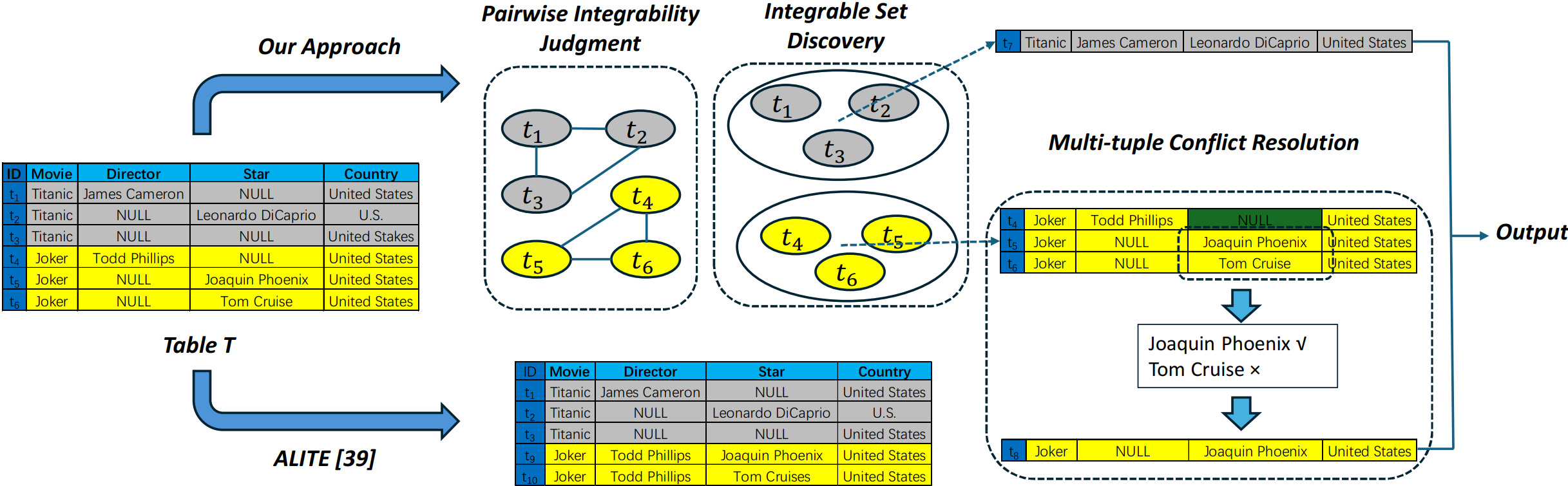
Figure 1. An example illustrating limitations in ALITE and our proposed approach.

Recently, a pioneering work called ALITE (Khatiwada et al., 2022) made the first attempt to integrate tables in data lakes. ALITE first focuses on the task of schema alignment, so the input tables can be safely combined into an intermediate table $T$, where the tuple’s value on attributes from other tables are denoted by missing values. Then, ALITE proceeds to integrate tuples in $T$ using a straightforward approach: if all the non-missing values on the shared attributes of two tuples are identical, they are integrated into a new tuple by substituting missing values with corresponding non-missing values from either tuple. While ALITE provides a solid foundation for subsequent tasks, it overlooks two critical yet commonly encountered cases in practice: 1) handling semantic equivalence and typographical errors, and 2) resolving conflicts during tuple integration.

Case 1: Semantic Equivalence and Typographical Errors. The tuples marked in grey in Fig. 1 are instances of semantic equivalence and typographical errors. Consider two tuples $t_{1}$ and $t_{2}$ in Table $T$ with values for the attribute Country as “United States” and “U.S.” respectively, which are semantically equivalent since they refer to the same entity. Ideally, $t_{1}$ and $t_{2}$ should be integrated. Furthermore, the value of the attribute Country in tuple $t_{3}$ is “United Stakes”, a typographical error of “United States” in $t_{1}$. Ideally, $t_{1}$ and $t_{3}$ should also be integrated. However, ALITE does not address issues like semantic equivalence or typographical errors, thereby limiting its effectiveness in integrating such cases.

Case 2: Conflicts are another key problem in multi-tuple integration, which requires careful resolution. As illustrated in Fig. 1, tuple $t_{4}$ can be integrated with either $t_{5}$ or $t_{6}$. However, when attempting to determine the missing value for the attribute Star in $t_{4}$, using the corresponding attribute values from $t_{5}$ or $t_{6}$ leads to conflicting possibilities: “Joaquin Phoenix” vs “Tom Cruise”. To resolve this conflict, an ideal solution should select the correct value, “Joaquin Phoenix” to fill the Star attribute in $t_{4}$. Unfortunately, ALITE does not provide mechanisms for conflict resolution. Hence, both pairs $(t_{4},t_{5})$ and $(t_{5},t_{6})$ are integrated independently, resulting in tuples $t_{9}$ and $t_{10}$, respectively. This fragmented approach can introduce incomplete or contradictory information into the integrated table, potentially impacting downstream tasks adversely.

To overcome these limitations, we propose a novel approach to integrate data lake tables that comprehensively tackles the three interconnected tasks: pairwise integrability judgment, integrable set discovery, and multi-tuple conflict resolution, whose workflow is illustrated at the top of Fig. 1.

In addressing the task of pairwise integrability judgment, our objective is to accurately predict the integrability of each tuple pair within a table $T$, even in the presence of semantic equivalence and typographical errors. Our solution starts from training a binary classifier, where a major challenge lies in the scarcity of labeled data specific to data lake tables. To mitigate this challenge, we adopt a strategy where semantic equivalence and typographical errors are treated as minor perturbations of each tuple $t$. We then employ data augmentation techniques along with adversarial examples to simulate these perturbations. This allows us to automatically generate a sufficient amount of training data to train a binary classifier, thereby overcoming the limitation imposed by the scarcity of labeled data.

For the task of integrable set discovery, we address it from two perspectives: 1) Each integrable set can be considered as a maximal clique in a graph constructed from table $T$, and hence, our objective is to find maximal cliques in an undirected graph. To this end, we propose to employ the well-known Bron-Kerbosch algorithm (Regneri, 2007) to find these integrable sets. 2) Recognizing that predictions from pairwise integrability judgment may contain errors, leading integrable sets may not strictly conform to a clique structure. Hence, we relax the connectivity criteria and view an integrable set as a densely connected subgraph, akin to a community. To handle this, we propose to employ community detection methods tailored for identifying such structures.

Finally, to solve the task of multi-tuple conflict resolution, we depart from conventional conflict resolution approaches in data fusion (Dong and Naumann, 2009; Li et al., 2014), which typically rely on extensive labeled data. Instead, we propose a novel method called in-context learning for conflict resolution (ICLCR). This method leverages the extensive knowledge embedded in pre-trained large language models (LLMs), which require only a few labeled demonstration examples to predict conflict resolution outcomes. This approach significantly reduces the dependency on large labeled datasets while maintaining comparable performance level. The effectiveness of our approach is closely linked to the number and quality of the demonstration examples. However, the input size limitations of an LLM limit the number of demonstration examples that can be used. To overcome this limitation, we propose an effective strategy for compressing demonstration examples, reducing the average number of tokens to represent an example, thereby enabling inclusion of more examples in a single input. Additionally, we introduce targeted strategies for selecting demonstration examples that are most relevant to the conflict resolution task, further enhancing the overall performance of our model.

In summary, our approach exhibits significant potential to enhance table integration within data lakes, offering the following contributions:

• To solve the task of pairwise integrability judgment, we propose a novel Self-Supervised Adversarial Contr- astive Learning framework, SSACL, to train a binary classifier with limited labeled data, to predict pairwise integrability of tuple pairs (Sec. 3).

• To solve the task of integrable set discovery, we propose two different yet related approaches. We explore existing solutions relevant to these problems to effectively support the task of integrable set discovery. (Sec. 4).

• To solve the task of multi-tuple conflict resolution, we develop an in-context learning-based method, namely In-context Learning for Conflict Resolution (ICLCR), which demonstrates promising performance with limited labeled data (Sec. 5).

• Since no suitable benchmarks exist to evaluate our problem, we have taken the initiative to create our owns and make it public. (Sec. 6).

• We conduct an extensive evaluation of our methods and compare it against suitable baselines on the new benchmarks. When comparing against the best-performing competitors, our SSACL exhibits a relative improvement of $4.2\%$ in terms of F1 on the task of pairwise integrability judgment, and ICLCR achieves a relative improvement of $18.9\%$ in Accuracy on the task of multi-tuple conflict resolution. Furthermore, both SSACL and ICLCR, when using limited labeled data, experience a decrease in performance of less than $10\%$, compared with when they are trained with a sufficient amount of labeled data. We also find that among all the methods proposed for integrable set discovery, Graph Neural Network (GNN) achieves the best performance. (Sec. 7).

2. Problem Formulation

In this section, we introduce the problem definition for the three tasks: pairwise integrability judgment, integrable set discovery, and multi-tuple conflict resolution. We assume the schema of the input tables to be integrated from data lakes have already been aligned, and they have been joined into an intermediate table $T$ using an outer union operator.

Definition 2.1.

Pairwise integrability judgment. Given a tuple pair $(t_{i},t_{j})$ that may be semantically equivalent or contain typographical errors, a function $f(t_{i},t_{j})$ outputs a $1$ or $0$, which indicates whether $t_{i}$ and $t_{j}$ are integrable or not.

After obtaining the pairwise integrability for all tuple pairs in table $T$, the next task is to identify all of the integrable sets in $T$, as defined in Def. 2.2.

Definition 2.2.

Integrable set discovery. Given a table $T$ and a pairwise integrability judgment function $f$, multiple disjoint integrable sets may be produced, denoted as $\mathcal{S}=\{S_{1},S_{2},...,S_{|\mathcal{S}|}\}$. Each integrable set $S$ ($S\in\mathcal{S}$) contains a collection of tuples that meet two conditions:

• Consistency. For any two tuples $t_{i}\in S,t_{j}\in S$, $f(t_{i},t_{j})=1$ should always hold.

• Maximality. For each tuple $t_{i}\notin S$, there should exist at least one tuple $t_{j}\in S$ such that $f(t_{i},t_{j})=0$.

For each integrable set $S\in\mathcal{S}$ that was discovered using Definition 2.2, all tuples in $S$ are considered to be integrable into a single tuple, and denoted as $t_{new}$. This integration process involves filling the attributes of $t_{new}$ with the correct value. However, when a certain attribute $t_{new}$ has multiple distinct values that originate from different tuples in $S$, we refer to it as a conflict, and multi-tuple conflict resolution formally addresses this condition.

Definition 2.3.

Multi-tuple conflict resolution. Given an integrable set $S$, a tuple $t_{new}$ is produced by integrating all tuples in $S$, such that: for each attribute $a$ in $t_{new}$, where a conflict exists, the correct value $v^{*}$ is chosen from the candidate set $C=\{t[a]|t\in S\land t[a]\neq NULL\}$ to complete the attribute value $t_{new}[a]$.

It is worth highlighting that the definition of pairwise integrability judgment shares similar spirit with entity resolution (Tu et al., 2022; Ebraheem et al., 2018), which aims to judge whether two tuples refer to the same entity. However, in our context, two tuples can be integrated even if they do not strictly correspond to the same entity. For instance, a tuple representing a movie and another representing a director can be integrated into a new tuple representing the director, where the movie acts as an attribute of the director tuple. Further distinctions between pairwise integrability judgment and entity resolution will be discussed in Sec. 8.

3. Pairwise Integrability Judgment

3.1. Key Idea

From Def. 2.1, it is clear that the pairwise integrability judgment function $f$ is a binary classifier, which outputs a $1$ or $0$ to indicate whether two tuples can be integrated. Thus, our goal is to derive a pairwise integrability judgment function $f$ using a machine learning model. For simplicity, we use $f$ to denote the pairwise integrability judgment function and a binary classifier interchangeably. However, a significant hurdle exists due to the unavailability of labeled data in data lake environments, and manually labeling data is prohibitively expensive.

To overcome this hurdle, we propose a novel approach – self-supervised adversarial contrastive learning (SSACL), which is designed to automatically generate training data for both positive and negative instances. For a given tuple $t$, although the negative instances (tuples that cannot be integrated with $t$) can be obtained using negative sampling (Awasthi et al., 2022; Armandpour et al., 2019), the key challenge is how to generate positive instances (tuples that can be integrated with $t$), particularly tuples that are semantically equivalent to tuple $t$ or exhibit typographical errors. To address this challenge, for each tuple $t$, we introduce a slight perturbation function $p$ to generate a positive instance $t^{+}$, i.e., $t^{+}=p(t)$. This slight perturbation function $p$ induces minimal semantic divergence from $t$ to $t^{+}$. Specifically, we employ two strategies to simulate $p$: data augmentation (Bayer et al., 2022; Feng et al., 2021; Wang et al., 2023) and adversarial examples (Ilyas et al., 2019; Zhang and Li, 2019; Goodfellow et al., 2014), which will be described in Sec. 3.2 and Sec. 3.5, respectively.

Naturally, for a tuple pair $(t,t^{+})$, $f(\boldsymbol{emb}(t),\boldsymbol{emb}(t^{+}))=1$ should hold. Once the model $f$ has been sufficiently trained on positive instances $(t,t^{+})$, accurately inferring the integrability of two tuples is plausible, even when the tuples are semantically equivalent or contain typographical errors. Furthermore, the binary classifier is trained using the contrastive learning framework, with the objective of producing embeddings where positive tuple pairs are closer together in the embedding space and negative tuple pairs are farther apart.

Fig. 2 presents the architecture for our proposed SSACL, which has the following main components:

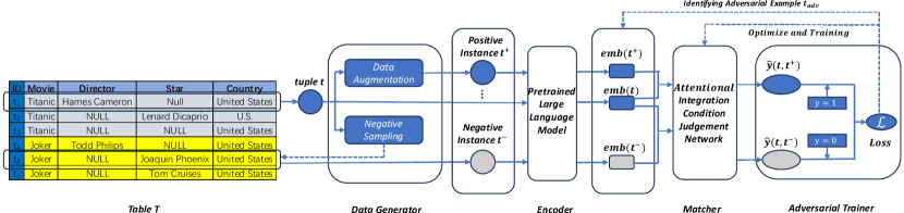
Figure 2. Architecture of our proposed SSACL

• The Data Generator introduces data augmentation and negative sampling to generate positive instances $t^{+}$ and negative instances $t^{-}$ for each tuple $t$, to form a training data set $\mathcal{D}_{train}$ (Sec. 3.2).

• The Encoder transforms each tuple $t\in\mathcal{D}_{train}$ generated from the data generator to a compact and semantically meaningful representation $\boldsymbol{emb}(t)$ (Sec. 3.3).

• The Matcher aims to match two tuples, which includes embeddings from the encoder as input, and outputs 1 or 0 to determine whether they are integrable or not (Sec. 3.4).

• The Adversarial Trainer is designed to create additional positive training instances using adversarial examples. Additionally, it can be used to optimize the parameters of matcher (Sec. 3.5).

3.2. Data Generator

A data generator automatically generates training data for pairwise integrability judgment. Specifically, for each tuple $t$, we use data augmentation techniques to produce a collection of perturbed tuples, $\mathcal{P}_{t}=\{t^{+}_{i}|t^{+}_{i}=p_{i}(t)\}$, where $p_{i}$ corresponds to a specific perturbation function. Consequently, every tuple pair $(t,t^{+}_{i})$ is a positive training instance for the matcher. Obviously, deciding how to create the slight perturbations $p_{i}$ impacts the quality of the training data, which in turn affects the performance of the training model $f$. So, the selection of perturbation functions should be comprehensive. Perturbation functions are carefully selected to adhere to two key principles (Shorten et al., 2021; Feng et al., 2021): (1) The perturbations should preserve the semantics of the original tuple $t$ or make minimal changes; (2) The perturbation functions should ideally cover a diverse range of possibilities to effectively represent multiple real-world scenarios. To achieve this, we develop a variety of perturbation functions which are organized into three types: attribute-level, word-level, and character-level.

Attribute-level. There are two kinds of attribute-level perturbations, namely attribute removal and attribute substitution.

• Attribute removal. This is applied to both numerical and text attributes. We randomly select an attribute value $a$ of a tuple $t$, and create a new tuple $t^{+}$ by removing its attribute value, $t^{+}[a]==NULL$. In all cases, $a$ is expected to be non-null.

• Attribute substitution. This is applied to text attributes only. We randomly select an attribute $a$ of a tuple $t$, and create a new tuple $t^{+}$ by using backtranslation methods (Edunov et al., 2018; Shorten et al., 2021), which generate a semantically equivalent description for $t[a]$, and use this new description to replace the original value $t[a]$. Backtranslation is a widely used data augmentation method in NLP to generate a sentence with similar semantics to the original sentence. The method first translates the sentence into a target language and then reverses the translation using a reverse model.

Word-level. There are three types of word-level perturbations – word removal, word substitution, and word swapping – all of them are applied to text attributes only.

• Word Removal. For a tuple attribute value, we randomly select a word and delete it.

• Word Substitution. For a tuple attribute value, we randomly select a word, and use WordNet (Miller, 1995) to find synonyms or hypernyms to form a candidate set. Finally, we randomly select a word from the candidate set to substitute the original term.

• Word Swapping. For a tuple attribute value, we randomly select two neighboring words, and swap their positions.

Character-level. For character-level perturbations, we simulate common typographical errors to create new tuples, which can be applied to both text attributes and numerical attributes. More details on how to simulate common typographical errors can be found in Table 1.

Specifically, for each original tuple $t$, we randomly select $N_{pos}$ perturbation functions to perturb the tuples $t^{+}$. In other words, we create $N_{pos}$ positive training instances for each original tuple $t$, and for negative training instances, we adopt the widely used strategy of negative sampling (Awasthi et al., 2022; Armandpour et al., 2019) to uniformly select $\mathcal{N}_{neg}$ tuples ($t$ to be excluded) at random in the training table for each tuple $t$.

Table 1. Typographical errors for textual Attributes

Error type	Description
char swap	Swap two random consecutive word characters in the text.
missing char	Skip a random word character in the text.
extra char	Add an extra, keyboard-neighbor, letter next to a random word character.
nearby char	Replace a random word character with keyboard-neighbor letter.
similar char	Replace a random word character with another visually similar character .
skipped space	Skip a random space from the text.
random space	Add a random space in the text.
repeated char	Repeat a random word character.
unichar	Replace a random consecutive repeated letter with a single letter.

Table 2. Typographical errors for numerical attributes

Error type	Description
digit swap	Swap two random consecutive digits in the number.
missing digit	Skip a random digit in the number.
extra digit	Add an extra, keyboard-neighbor, digit next to a random digit in the number.
nearby digit	Replace a random digit in the number with a keyboard-neighbor digit.
similar digit	Replace a random digit with another visually similar digit.
repeated digit	Repeat a random digit in the number.
unidigit	Replace a random consecutive repeated digit with a single digit.

3.3. Encoder

Given a tuple $t$, an encoder learns a compact and semantically meaningful embedding $\boldsymbol{emb}(t)$ to represent $t$. In this paper, we adopt attribute-level representations for each tuple, enabling us to perform fine-grained comparisons for the attribute values from any two tuples. Specifically, for each tuple, $t$, the encoder encodes the following representation:

(1) $$\boldsymbol{emb}(t)=[\boldsymbol{emb}(t[a_{1}]),\boldsymbol{emb}(t[a_{2}]),...,\boldsymbol{emb}(t[a_{m}])].$$

Here, $m$ denotes the number of attributes in Table $T$, $t[a_{i}]$ represents the value of the attribute $a_{i}$ in the tuple $t$, and $\boldsymbol{emb}(t[a_{i}])$ denotes the corresponding embedding. Note that for a tuple $t$, there may be missing attributes. To handle such cases, we use a special token $[NULL]$ to mark missing values, which will also be mapped to an embedding. Furthermore, for each tuple $t$, we also create a masking vector $\boldsymbol{Mask}(t)$ that has $m$ dimensions:

(2) $$\boldsymbol{Mask}(t)=[d_{1},d_{2},...,d_{m}],$$

where we set the $i\cdot$th element of the masking vector $d_{i}$ to 0 if the corresponding attribute value for tuple $t$ is missing; otherwise, we set it to 1. The masking vectors are discussed further in Sec. 3.4.

To obtain $\boldsymbol{emb}(t[a_{i}])$, we first serialize an attribute value $t[a_{i}]$ into a sequence of words. Then, for each word $w$ in the sequence, we generate an embedding using a pretrained language model. There are two different embedding methods, namely word-level embeddings such as word2vec (Mikolov et al., 2013) and GloVE (Pennington et al., 2014), and subword-level embeddings such as FastText (Bojanowski et al., 2017) and BERT (Kenton and Toutanova, 2019). Word2vec encodes each term individually and uses an embedding vector to represent it, whereas GloVE tokenizes a word into a sequence of subwords and represents each subword using an embedding. In this work, we use a subword-level embedding method. This choice is driven by their capability to handle unknown and uncommon terms, while also exhibiting greater resilience to typographical errors.

For every sequence of tokens, the respective token embeddings are aggregated into a single embedding vector. We adopt a transformer-based architecture (Kenton and Toutanova, 2019) for this aggregation process. This choice stems from their proven ability to adeptly capture contextual information embedded in sequences in the transformer. As a result, we obtain an embedding $\boldsymbol{emb}(t[a_{i}])$ tuned for the matcher, which we will discuss in Section 3.4.

3.4. Matcher

Given the embedding representation for two tuples $\boldsymbol{emb}(t_{1})$ and $\boldsymbol{emb}(t_{2})$, the matcher outputs 1 or 0, indicating whether the two tuples should be integrated. One straightforward way to achieve this is to compute the cosine similarity between $\boldsymbol{emb}(t_{1})$ and $\boldsymbol{emb}(t_{2})$, or concatenate the two embeddings into a Multi-layer Perceptron (MLP). A common drawback emerges from the uniform treatment of every attribute, which ignores any potential variations in the contributions to the semantic correctness for a given tuple.

To overcome this drawback, we propose an Attentional Integrability Judgment Network (AIJNet), which assigns different weights to the attributes in the matching process. Specifically, for two embeddings $\boldsymbol{emb}(t_{1})$ and $\boldsymbol{emb}(t_{2})$, we first concatenate both into a single embedding: $\boldsymbol{emb}(t_{1},t_{2})=[\boldsymbol{emb}(t_{1}),\boldsymbol{emb(t_{2})}]$ . Next, we consider the varying importance of each attribute and reformulate the representation of the tuple pair $(t_{1},t_{2})$ using a self-attention mechanism (Vaswani et al., 2017):

(3) $$\boldsymbol{emb}^{*}(t_{1},t_{2})_{i}=\sum_{j=1}^{2m}\text{softmax}\left(\boldsymbol{Mask}(t_{1},t_{2})_{j}\frac{\boldsymbol{Q}_{i}\cdot\boldsymbol{K}_{j}^{T}}{\sqrt{d_{k}}}\right)\cdot\boldsymbol{V}_{j}.$$

Here, $\boldsymbol{emb}^{*}(t_{1},t_{2})$ is the final representation of the tuple pair $(t_{1},t_{2})$, $d_{k}$ represents the size of each attribute embedding, and $\boldsymbol{Mask}(t_{1},t_{2})$, is the concatenation of $\boldsymbol{Mask}(t_{1})$ and $\boldsymbol{Mask}(t_{2})$, is used to mask the impact of a missing attribute value relative to other attributes. $\boldsymbol{Q},\boldsymbol{K},\boldsymbol{V}$ are the query matrix, the key matrix, and the value matrix, respectively, which are computed using a linear transformation (Vaswani et al., 2017).

Finally, $\boldsymbol{emb}^{*}(t_{1},t_{2})$ is the input, and we use an MLP to output a binary decision $y$, indicating whether $t_{1}$ and $t_{2}$ can be integrated.

3.5. Adversarial Trainer

The adversial trainer serves dual purposes: (1) Establish a contrastive training objective optimized using an SGD-based algorithm; (2) Identify adversarial examples to further enrich the training set. Next, we will explain this idea in detail.

Objective Function. In this work, we use a binary noise contrastive estimation (NCE) loss function (Khosla et al., 2020) for the training objective, which is formulated as:

(4) $$\mathcal{L}=\sum_{i=1}^{N}(\sum_{j=1}^{N_{pos}}log~f(t_{i},t^{+}_{ij})+\sum_{j=1}^{N_{neg}}log~f(t_{i},t^{-}_{ij})).$$

Here, $N$ is the total number of tuples in the training table, and $t_{ij}^{+}$ and $t^{-}_{ik}$ denote one positive instance and negative instance for the tuple $t_{i}$, respectively. The optimization of the NCE loss function enables the model to make similar tuples that are close in the embedding space while scattering dissimilar tuples.

Adversarial Examples and Training. We propose the use of adversarial examples (Ilyas et al., 2019; Zhang and Li, 2019) to further enrich the pool of positive training instances for our model. Technically speaking, an adversarial example is typically viewed as a perturbed version of the original input example, which results in a significant impact in a decision made by a machine learning model. Conversely, perturbations in data augmentation that operate on the original tuples while perturbations in adversarial training directly impact the embedding vectors, expressed as:

(5) $$p(\boldsymbol{emb}(t_{i}))=\boldsymbol{emb}(t_{i})+\boldsymbol{r},$$

where $\boldsymbol{r}$ denotes the perturbation vector. Since the adversarial example has the most significant impact on model performance, this can also be expressed as the following objective function:

(6) $$max_{\boldsymbol{r}}\mathcal{L}(f(t_{i},t_{i}^{adv}),y_{i}),s.t.||\boldsymbol{r}||_{2}<\epsilon.$$

Here, $\epsilon$ is a small value that constrains the magnitude of the perturbation, $y_{i}$ is set to 1 since the pair of original tuples and the corresponding adversarial example $(t_{i},t^{adv}_{i})$ should consistently result in a positive prediction.

Since $r$ is very small, the loss function is approximately equivalent to the following equation derived using a first-order Taylor approximation (Nocedal and Wright, 2006):

(7) $$\mathcal{L}(f((t_{i},t_{i}^{adv}),y_{i})\approx\mathcal{L}(f((t_{i},t_{i}),y_{i})+\nabla_{t_{i}}\mathcal{L}(f((t_{i},t_{i}),y_{i})^{T}\boldsymbol{r}.$$

When using a Lagrange Multiplier Method (Boyd and Vandenberghe, 2004) to solve Eq. 6 and Eq. 7, we get:

(8) $$\boldsymbol{r}=-\epsilon\frac{\nabla_{t_{i}}\mathcal{L}(f((t_{i},t_{i}),y_{i})}{||\nabla_{t_{i}}\mathcal{L}(f((t_{i},t_{i}),y_{i})||^{2}}$$

Consequently, for each tuple $t$, we can derive an adversarial example $t_{i}^{adv}$. This process is repeated in each training epoch, with $(t_{i},t_{i}^{adv})$ being added to the positive training instance pool.

Once we have trained the model $f$, it can be employed to assess the pairwise integrability of any tuple pair in the table $T$. Similarly to entity resolution, this process can be expedited through the use of blocking techniques (Ebraheem et al., 2018; Thirumuruganathan et al., 2021). These techniques partition tuples into distinct blocks, allowing for pairwise comparisons exclusively within each block, thereby enhancing computational efficiency.

4. Integrable Set Discovery

Given the integrability of any two tuples in Table $T$, determined using a binary classifier, this section introduces how to derive all possible integrable sets within $T$. Most existing studies, such as ALITE (Khatiwada et al., 2022), are limited to integrating two tuples in each step of the algorithm. This restricts their ability to include additional tuples that could potentially resolve conflicts within larger sets. In contrast, our objective is to integrate multiple tuples simultaneously, enabling the detection and resolution of conflicts as they arise. Therefore, our goal is to identify all integrable sets within Table $T$, where each integrable set refers to a set of tuples that can be integrated, as defined in Def. 2.2. As discussed in Sec. 2.2, each integrable set found in table $T$ should meet the criteria of consistency and maximality. To achieve this, we can frame the task of integrable set discovery as the problem of identifying all maximal cliques in a graph, as described below.

Integrable Set Discovery by Finding Maximal Cliques. To discover integrable sets within each table $T$, we proceed with constructing an undirected graph $\mathcal{G}=\{\mathcal{V},\mathcal{E}\}$ from $T$ in two steps: 1) each tuple $t_{i}$ is represented as a node $v_{i}\in\mathcal{V}$; 2) for every tuple pair $(t_{i},t_{j})$, if the binary classifer $f(t_{i},t_{j})=1$, an edge $e_{ij}\in\mathcal{E}$ is created. Once $\mathcal{G}$ is constructed, the task of integrable set discovery transforms into finding all maximal cliques in $\mathcal{G}$. In graph theory, a clique is a subset of vertices in an undirected graph such that every pair of vertices in this subset is connected by an edge, and a maximal clique in a graph is a clique that cannot be extended by adding another adjacent vertex from the graph. Thus, there exists a one-to-one mapping from each integrable set in table $T$ to each maximal clique in graph $\mathcal{G}$.

This allows us to leverage graph algorithms designed for clique detection to efficiently find all possible integrable sets within $T$. One of the most commonly used algorithms is the Bron-Kerbosch algorithm (Regneri, 2007), which employs recursive backtracking and uses a pivot selection strategy to efficiently explore and prune the search space. Algorithm 1 outlines the key steps of the Bron-Kerbosch algorithm, in which three sets $R$, $P$, and $X$ are used: $R$ denotes the current clique being constructed; $P$ denotes the set of the candidate vertices that can potentially be added to $R$; $X$ denotes the set of vertices that have already been excluded from consideration. The algorithm proceeds as follows: If both $P$ and $X$ are empty, then $R$ is a maximal clique, and the algorithm will output $R$ (Lines 2-4). Then, we select a pivot vertex $v_{i}$ from $P\cup X$ (Line 5). For each vertex $v_{j}\in P$ that is not adjacent to $v_{i}$, we add $v_{j}$ to $R$ and intersect both $P$ and $X$ with the neighbors of $v_{j}$ (Lines 6-7). After exploring all vertices in $P$ that are not adjacent to $v_{i}$, each vertex $v$ is moved to $X$ and the algorithm continues (Lines 8-9).

1

2Function BronKerbosch($R,P,X$):

3    if $P$ is empty and $X$ is empty then

4       Output: $R$;

5      

6    end if

7   $u\leftarrow$ ChoosePivot($P\cup X$);

8    foreach $v\in P\setminus N(u)$ do

9       BronKerbosch($R\cup\{v\},P\cap N(v),X\cap N(v)$);

10       $P\leftarrow P\setminus\{v\}$;

11       $X\leftarrow X\cup\{v\}$;

12      

13    end foreach

14   

15

16

Algorithm 1 Bron-Kerbosch Algorithm

Integrable Set Discovery using Community Detection. In theory, Algorithm 1 can accurately identify all integrable sets from table $T$ if the integrability of any tuple pair in $T$ can be correctly predicted. However, Algorithm 1 is not empirically robust for our problem. Consider an integrable set $S$ exists and a tuple $t_{i}\in S$ should be integrable with any other tuple $t_{j}\in S$. If SSACL incorrectly determines the integrability of $t_{i}$ and any other tuple $t_{j}\in S$, Algorithm 1 may fail to add $t_{i}$ into $S$, even if the integrability of $t_{i}$ and other tuples $t_{k}\in St_{k}\neq t_{j}$ can be correctly decided. To address this issue, we relax the topographical requirement of an integrable set in graph $\mathcal{G}$ in practice. Instead of requiring that each tuple pair in an integrable set is judged as integrable by SSACL, we focus on ensuring that each tuple within an integrable set is integrable with any other tuple in the same set. This approach transforms the task of multi-tuple conflict resolution into a community detection problem, which aims to identify densely interconnected groups or clusters of nodes within the graph. In this work, we have chosen a collection of representative community detection methods and applied them to address the task integrable set discovery, as outlined below:

• The Louvain (Blondel et al., 2008) algorithm is a modularity-based method that iteratively optimizes the modularity to find a partition of the network that maximizes the quality of the community structure.

• Newman-Girvan (Newman and Girvan, 2004) algorithm is a hierarchical clustering method that hierarchically removes edges with “high betweenness centrality” to identify communities.

• Infomap (Rosvall and Bergstrom, 2008) is an information theoretic approach that minimizes the description length of a random walk path through the network to uncover communities.

• Spectral Clustering (Ng et al., 2001) uses eigenvectors from a graph Laplacian matrix to partition nodes into clusters.

• Graph Neural Network (GNN) (Bruna and Li, 2017) is a DL-based representative learning approach that aims to leverage graph neural networks to learn meaningful representations of nodes based on the topographical structure and attributes, which are then used to cluster nodes into different communities.

As we shall see shortly in Sec. 7, we will evaluate the effectiveness and efficiency of each method above in addressing the task of integrable set discovery.

5. Multi-tuple Conflict Resolution

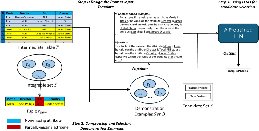
Figure 3. The workflow of ICLCR

5.1. Key Idea

Based on pairwise integrability judgment, we obtain a collection of integrable sets $\mathcal{S}$. For each integrable set $S\in\mathcal{S}$, we integrate all of the tuples contained in $S$ in a single tuple $t_{new}$, which provides more comprehensive information than each individual tuple $t\in S$. Thus, the question now is how to determine the correct attribute value $t_{new}[a]$ for an attribute $a$, which can fall into one of three potential categories:

• Non-missing Attributes. An attribute $a$ is considered non-missing if $t[a]\neq NULL$ for any $t\in S$. To populate $t_{new}[a]$, we randomly select a tuple $t\in S$ and use its attribute value $t[a]$. This approach is appropriate because, in the context of pairwise integrability judgment, all tuple values for a non-missing attribute $a$ possess equivalent semantics within the integrable set.

• Missing Value Attributes. An attribute $a$ is considered as a missing value attribute if $t[a]==NULL$ for all $t\in S$. In this case, $t_{new}[a]$ is assigned a $NULL$ value. This choice is made due to the absence of any reliable information to populate $t_{new}[a]$.

• Partially Missing Attribute. An attribute $a$ is considered partially missing if at least one tuple $t_{i}\in S$ has $t_{i}[a]==NULL$ and at least one tuple $t_{j}\in S$ has $t_{j}[a]\neq NULL$. Given the heterogeneous nature of the data in the input tables, non-null values for multiple tuples on the attribute $a$ may conflict with each other, resulting in a candidate set $C(a)=\{t[a]|t\in S\land t[a]\neq NULL\}$. To resolve this, we must select the correct value $v^{*}\in C$ to fill $t_{new}[a]$.

The first two types of attributes can be resolved easily, and hence we focus on how to fill partially missing attributes. This can be formulated as a conflict resolution problem, as articulated in Definition 2.3. Existing solutions for conflict resolution in the context of a data fusion problem rely on truth discovery approaches (Li et al., 2012, 2014; Zhi et al., 2015), which first estimate the trustworthiness of a data source, and subsequently choose the value from the most reliable source to fill a missing value. However, truth discovery approaches typically rely on a lot of training data or metadata (i.e., paper citation and reviews) in order to estimate the reliability of the source. This imposes limitations on the applicability of these methods, as practical scenarios often lack access to sufficient labeled data, and obtaining such data requires considerable human curation and financial burdens.

To address this problem, we propose a novel method for conflict resolution, namely In-context Learning for Conflict Resolution (ICLCR). This method draws inspiration from the recent success of in-context learning (ICL) within the field of natural language processing (Min et al., 2022; Xie et al., 2021; Akyürek et al., 2022) . ICL-based methods solve downstream tasks by leveraging contextual information provided by an input prompt, removing the necessity for explicit task-specific training. This approach allows large language models (LLMs) to dynamically adapt their behavior based on a few labeled demonstration examples and instructions embedded in the prompt. Intuitively, applying ICL-based methods to our conflict resolution problem should effectively mitigate the issue of insufficient amount of labeled data. These methods primarily utilize large language models (LLMs) that are pretrained on the extensive corpora, and therefore accumulate a broad spectrum of knowledge. Conversely, in private domains not covered by the training corpora, ICL-based methods require only a few examples to adapt and perform effectively.

However, applying in-context learning (ICL) methods to our conflict resolution problem presents several challenges. Technically, the effectiveness of these methods heavily depends on the selection of demonstration examples. While ICL-based methods typically require only a small number of demonstration examples, including more examples can provide LLMs with richer contextual information for handling downstream tasks effectively. However, the constrained input size of current LLMs limits the number of demonstration examples that can be feasibly incorporated. Thus, a key challenge is to maximize the number of demonstration examples within the given input size constraints. Furthermore, given the restricted number of demonstration examples that can be selected, it becomes crucial to prioritize those that are most relevant to the specific aspects of the downstream task. This ensures that the model can effectively learn and generalize from the provided examples, thereby enhancing its ability to resolve conflicts accurately.

To address the above challenges in leveraging ICL-based methods for conflict resolution, ICLCR relies on two key strategies: demonstration example compression and selection. Specifically, in demonstration example compression, non-relevant attributes that contribute minimal information to the prediction of target attributes are ignored when transforming a tuple into a natural language sentence. This reduces the number of tokens to express each demonstration example. Furthermore, in demonstration example selection, we judiciously choose the demonstration examples that are semantically similar to the target, ensuring that the most relevant examples are included.

Fig. 3 illustrates the workflow of our proposed ICLCR, which mainly consists of three steps that apply in-context learning to solve the conflict resolution problem:

• Step 1: Designing the Prompt Input aims to transform the task of conflict resolution into a prompt input that can be resolved using an LLM.

• Step 2: Compressing and Selecting Demonstration Examples aims to select the most instructive tuples from the intermediate table $T$ as the demonstration examples.

• Step 3: Using LLMs for Candidate Selection mainly adopts a pre-trained LLM to predict which values in the candidate set has the largest possibility given the prompt input.

5.2. Designing the Prompt Input Template

The first step is to transform the problem of conflict resolution into a prompt input (or context) $P$ with several demonstration examples, which can be formally expressed as $P=\{x_{1},y_{1},x_{2}$, $y_{2},...,x_{k},y_{k},\hat{x},\hat{y}\}$, where $x_{i}$ and $y_{i}$ denotes an answer and a question in the form of natural language sentence, respectively, jointly constituting a demonstration example $d_{i}$. $\hat{x}$ is the target question and $\hat{y}$ is the undecided answer.

In this problem, for an integrable set $S$, to fill a partially missing attribute $a_{par}$ in $t_{new}$, at most $k$ tuples are selected as demonstration examples to instruct LLMs to make prediction for $t_{new}[a_{par}]$. To enable LLMs to understand the demonstrate example, we need to transform each selected tuple $t$ into a natural language sentence composed of $x_{i}$ and $y_{i}$. To accomplish this, for each demonstration tuple $t_{i}$, we adopt the following template to transform it into a natural language sentence:

Demonstration Example Template. For a tuple, if the values of an attribute __ is __ , the attribute __ is __, …, respectively, then the value of the attribute __ should be __.

In detail, to transform a tuple $t_{i}$ into a demonstration example $d_{i}$ in terms of making prediction on $a_{par}$ in an integrable set $S$, each of its non-missing attribute names (except for the partially-missing attribute $a_{par}$ in $S$) and the corresponding values should be used to fill the blank in the “if” clause, forming $x_{i}$, and the name of the partially attribute $a_{par}$ and the value on $a_{par}$ of $t_{i}$ are used to fill the blank in the “then” clasue, forming $y_{i}$. Similarly, each of its non-missing attribute names of $a_{new}$ and the corresponding values should be used to fill the blank in the “if” clause, forming $\hat{x}$, while the blank for the attribute value in the “then” clause should be left out, which will be answered by an LLM. Thus, all demonstration examples along with the target question constitute the prompt input $P$. Next, we further illustrate how to judiciously select demonstration examples to populate the input prompt $P$.

5.3. Compressing and Selecting Demonstration Examples

Demonstration examples are labeled data that instruct LLMs how to make predictions for a given task. The choice of demonstration examples, denoted as $D$, has a significant impact on the effectiveness of in-context learning. Intuitively, the model performance of ICLCR is closely relevant to two factors: 1) the number of demonstration examples $N$ in the prompt input $P$; 2) the relevance of the demonstration examples in $D$ to the target question $q$ transformed from $t_{new}$. To address these two issues, in this paper, we propose effective demonstration example compression and selection strategies in Section 5.3.1 and Section 5.3.2, respectively.

5.3.1. Demonstration Example Compression

Since the input size of an LLM is limited, it is impossible to include as many demonstration examples in the prompt input $P$ as desired. Thus, a key challenge here is how to include as many demonstration examples in the prompt input $P$ as possible. To address this problem, we propose a demonstration example compression strategy. Intuitively, if we want to include as many demonstration examples in $P$ as possible, one solution is to minimize the average number of tokens to express a demonstration example in the natural language sentence while maintaining the information about the target attribute. Note that when we transform a tuple $t_{i}$ into a demonstration example $d_{i}$, the length of $d_{i}$ is roughly proportional to the number of the non-missing attributes in $t_{i}$. Note that not all non-missing attributes contribute to the prediction of $a_{par}$. For example, the ID number is not relevant and can be ignored if we want to make a prediction on the position of a person. Thus, if we can remove all the non-relevant attributes for $a_{par}$, the average length of demonstration examples can be greatly reduced, and more demonstration examples can be included in the prompt input $P$ to instruct LLMs to achieve better performance. Note that even in the case where the maximum number of demonstration examples that can be included in the prompt input is larger than the number of available labeled demonstration examples, the proposed demonstration example compression strategy is still helpful because it reduces the length of prompt input, and the inference time of LLMs can be reduced, improving the overall efficiency.

Then, to quickly and effectively decide whether a non-missing attribute $a_{non}$ is not relevant when predicting $a_{par}$, the mutual information (MI) metric can be used, which is widely used to capture the relationship and dependency between two variables. Formally, given two variables $X$ and $Y$, their mutual information is calculated using

(9) $$~I(X;Y)=\sum_{x\in X}\sum_{y\in Y}p(x,y)\log\left(\frac{p(x,y)}{p(x)p(y)}\right),$$

where $p(x,y)$ denotes the joint distribution possibility for $X=x$ and $Y=y$, and $p(x)$ and $p(y)$ denote the marginal distribution for $X$ and $Y$, respectively. Specifically, a large $I(X;Y)$ indicates that there is a strong dependence between $X$ and $Y$ and when $I(X;Y)$ is close to 0, it means that there is no dependency between the two variables.

In this paper, we utilize Eq. 9 to calculate the dependency between a non-missing attribute $a_{non}$ and a partially-missing attribute $a_{par}$. Since Eq. 9 only applies to discrete variables, we process different attribute types as follows: 1) Categorical and text attributes are transformed into discrete values based on their distinct values; 2) Numerical attributes are converted into discrete values by binning them into intervals. Then, we apply a small value $\beta=0.1$ as the threshold to decide if the two attributes are dependent. Specifically, if $I(a_{par};a_{non})<\beta$, we remove the corresponding description for the non-missing attribute $a_{non}$ in the demonstration example template.

5.3.2. Demonstration Example Selection

The choice of demonstration examples also provide important performance improvements for the LLMs during conflict resolution. It is desirable to choose the tuples that are most relevant to the new tuple $t_{new}$ as demonstration examples. In this paper, we investigate three different demonstration selection strategies, namely a random selection strategy, a $K$-NN selection strategy, and a weighted $k$-NN selection strategy, respectively.

Random Selection. An intuitive and simple strategy is to randomly choose $k$ tuples from the intermediate table $T$ as demonstration examples. However, since the demonstration examples are randomly selected from $T$, it is likely that they contain limited information to help make a prediction for $a_{par}$ and $t_{new}$.

$k$-NN Selection. To address problem faced by random selection above, we select tuples that are semantically close to $t_{new}$ as demonstration examples. To accomplish this goal, we compute the cosine similarity using an embedding-based representations of a candidate tuple $t$ and the new tuple $t_{new}$. Specifically, for each integrable set $S\in\mathcal{S}$, an initial $t_{new}$ is derived by collating all available values from non-null attributes within the integrable set, which produces a set of multiple $t_{new}$ of size $|\mathcal{S}|$. Furthermore, we encode each $t_{new}$ using Eq. 1 to generate an encoded representation $\boldsymbol{emb}(t_{new})$, and then compute the average embedding $\overline{\boldsymbol{emb}(t_{new})}$ for all $\boldsymbol{emb}(t_{new})$ of size $|\mathcal{S}|$. Next, we perform a $k$-NN search to identify the $k$ tuples from table $T$ that are the most similar to $\overline{\boldsymbol{emb}(t_{new})}$ to the demonstration examples.

Weighted $k$-NN Selection. While the $k$-NN selection strategy is able to select relevant demonstration examples, as described in Sec. 5.3.1, different attributes in a candidate tuple $t$ can have different degrees of impact when predicting $a_{par}$, which cannot be determined using $k$-NN selection alone. To this end, we further improve $k$-NN selection by weighting different attributes using their normalized mutual information with the non-missing attribute $a_{par}$ when we aggregate the attribute representations into the tuple representation.

5.4. Using LLMs for Candidate Selection

With the design of the prompt input template and the selected demonstration examples, we can obtain the entire prompt input $P$, and ask a pre-trained LLM to answer the question – filling in $\hat{y}$. Here, the set of candidate values $C$ for $\hat{y}$ is composed of tuples whose values on $a_{par}$ are not missing. Then, a large language model (LLM) is used to predict which candidate value $v\in C$ has the highest likelihood of appearing in the prompt input $P$. This can be defined as $max_{v\in C}P_{LLM}(\hat{y}=v|P)$. In Sec. 7, we investigate the performance of various LLMs for the conflict resolution task.

6. Data Preparation and Evaluation

This section describes how to create the benchmarks, followed by the evaluation framework used in our experiments.

An ideal benchmark must exhibit two critical characteristics: (1) Every dataset should contain semantic equivalence cases, typographical errors, and conflicts, all of which we aim to address; (2) A dataset should be accompanied by definitive ground-truth annotations that label integrable sets and candidate values during conflict resolution, in order to facilitate a thorough effectiveness evaluation of our proposed solution. Given the presence of the first characteristics, directly using the test collection proposed for ALITE (Khatiwada et al., 2022), the most closely related work to ours, is not sufficient since errors and conflicts are not supported in ALITE. Thus, we have created our own benchmarks by injecting semantic equivalences, typographical errors, and conflicts, and recording ground-truth annotations for the evaluation. In Sec. 6.3, we also discuss why benchmarks from related tasks, such as entity resolution and conflict resolution, are not suitable for our problem.

6.1. Benchmark Creation

We create our benchmarks using two dataset repositories from ALITE (Khatiwada et al., 2022), Real and Join (Khatiwada et al., 2022). Both dataset repositories contain multiple datasets, each of which contains a set of input tables to be integrated.

Furthermore, we perform an outer-union operator (Khatiwada et al., 2022; Bleiholder et al., 2010) to join the tables in each dataset and produce a single intermediate table $T$, which is used to create our benchmarks. For each dataset repository, all the datasets are divided into three categories according to the size of the number of intermediate tables $T$, namely Small, Medium, and Large. Larger datasets generally contain more tuples, making them intuitively more difficult to handle. Table 3 provides additional statistics of the two dataset repositories used in the benchmark.

Table 3. The statistics of the two dataset repositories

		#Datasets	#Avg. Input Tables	#Avg. Columns	#Avg. Tuples
Real	Small	4	9.5	27	1524.2
	Medium	4	9	18	6902.5
	Large	3	9.3	12	48617.5
Join	Small	9	5	9.2	4578.2
	Medium	9	12.5	8.5	33704.4
	Large	10	15.8	13.7	77351.2

6.1.1. Noise Injection

First, we inject noise into the clean table $T$, so as to simulate semantic equivalence and typographical errors using a pre-define error rate. Since the datasets used in the literature for data cleaning (Abedjan et al., 2016; Peng et al., 2022) have a noise rate between 5% and 40%, we set the default noise rate to 30% in our experiments. Furthermore, we test three different settings for the ratio between semantic equivalence and typographical errors, 10%$/$20% (SE-heavy, short for semantic equivalence-heavy), 15%$/$15% (Balanced), and 20%$/$10% (TE-heavy, short for typographical error-heavy). Unless specified otherwise, we use the balanced noise case by default.

• Semantic Equivalence. Backtranslation (Edunov et al., 2018; Shorten et al., 2021) has been widely employed to generate sentences that maintain similar semantic meaning to the original sentence in the field of natural language processing. Once a cell is chosen for noise injection, we use backtranslation (Edunov et al., 2018; Shorten et al., 2021) to generate an alternative description with similar meaning to replace the original value. If the backtranslated description is the same as the original one, we randomly select a word in the original description and use WordNet (Miller, 1995) to generate a synonym or hypernym to replace it. We only inject this type of noise in text attributes.

• Typographical Errors. We simulate typographical errors in a comprehensive way, such as character swapping and character deletion. We inject typographical errors for both text and numerical attributes.

6.1.2. Conflict Generation

To generate conflicts, for each integrable set in $T$ (we will introduce how to obtain the ground-truth integrable set below), we choose one partially-missing text attribute $a$ (introduced in Sec. 5), and a tuple $t$ that has a non-null value for the attribute $a$. We use tuple $t$ as a template to generate the conflict tuples. Specifically, we assume that the conflict tuples come from different resources, each of which has a reliability score $r$ between 0 and 1. Then, we randomly replace $t[a]$ with another value from the other values in the attribute $a$ with a probability $1-r$. Using this strategy, we create 3-5 conflict tuples for each integrable set. We set $r_{i}$ to a random value between 30%-80%.

6.1.3. Ground-truth

We also need to create the ground-truth for our benchmarks. For multi-tuple integration, we use ALITE (Khatiwada et al., 2022) to integrate tuples in an error-free and conflict-free manner. During the integration, we track tuple pairs that are integrated, which are considered to be part of the ground-truth. Then based on the results from from ALITE, we use the Bron-Kerbosch algorithm to find the integrable sets in $T$. Note that the Bron-Kerbosch algorithm produces correct results in this case, as the input of pairwise integrability is the ground truth. Thus, in our benchmarks, the ground-truth can be generated by obtaining the tuples that form the integrable sets. For conflict resolution, the template tuple value $t[a]$ for the attribute $a$ is the ground-truth since we create the conflict tuples based on the tuple $t$.

6.2. Evaluation Metrics

Metrics for The Task of Pairwise Integrability Judgment.  Pairwise integrability judgment serves a similar purpose to the entity resolution task (Ebraheem et al., 2018; Li et al., 2020; Mudgal et al., 2018), so we use F1 to evaluate our results, and is expressed as the harmonic mean of $Recall$ and $Precision$, denoted as $F_{1}=2\times\frac{Recall\times Precision}{Recall+Precision}$. Here, $Recall=\frac{T_{P}}{T_{P}+F_{N}},Precision=\frac{T_{P}}{T_{P}+F_{P}}$, where $T_{P}$ denotes the number of integrable tuple pairs that are determined to be integrable, $F_{N}$ represents the number of integrable tuple pairs that are incorrectly determined to be non-integrable, and $F_{P}$ indicates the number of tuple pairs that are not integrable but determined to be integrable.

Metric for The Task of Integrable Set Discovery.  Given a set of ground-truth integrable sets $\mathcal{R}=\{R_{1},R_{2},...,R_{n}\}$ and a set of integrable sets $\mathcal{S}=\{S_{1},S_{2}$, $...,S_{m}\}$, we use the Similarity between $\mathcal{R}$ and $\mathcal{S}$ as the evaluation metric. Similarity is defined as the maximum weighted matching score in a bipartite graph, which has two disjoint sets of vertices $\mathcal{R}$ and $\mathcal{S}$, and a set of edges $(R_{i},S_{j})$ between any two vertices from $\mathcal{R}$ ($R_{i}\in\mathcal{R}$) and $\mathcal{S}$ ($S_{j}\in\mathcal{S}$), respectively. The weight of each edge $(R_{i},S_{j})$ is computed using Jaccard similarity, whenre $J=\frac{|R_{i}\cap S_{j}|}{|R_{i}\cup S_{j}|}$.

Metric for The Task of Multi-tuple Conflict Resolution.  We evaluate several methods in terms of Accuracy, which is the ratio computed by dividing the number of correctly filled attributes by the total number of conflict attributes available.

6.3. Further Discussion on Other Benchmarks

Although previous work (Li et al., 2012; Mudgal et al., 2018; Ebraheem et al., 2018) on entity resolution and conflict resolution provide test collections, they cannot be used in our experiments for the following reasons: (1) In most entity resolution benchmarks (Ebraheem et al., 2018; Li et al., 2020), a tuple can be matched with another tuple, which means each integrable set contains only two tuples and there is no need for conflict resolution. (2) Since $T$ is obtained using an outer-union operator (Khatiwada et al., 2022; Bleiholder et al., 2010) by using several tables of different schemas, it usually produces many missing values, while in test collections for entity resolution, there are usually a small number of missing values. This makes it difficult to compare directly using these methods. (3) Most entity resolution studies have only a few attributes in the test collection. For example, DBLP-scholar (Tu et al., 2023; Li et al., 2020), one of the most widely used test collection for entity resolution, has only five attributes, while the average number of attributes in the datatsets in Real and Join dataset repositories are 19.6 and 10.6 per table on average, respectively.

7. Experiments

First, we evaluate the effectiveness of the proposed methods for the three core tasks studied in this work: pairwise integrability judgment, integrable set discovery, and multi-tuple conflict resolution (Sec. 7.2). Second, considering that the proposed SSACL and ICLCR are designed to be effective using limited labeled data, we assess the performance under this constraint (Sec. 7.3). Third, we investigate the impact of various choices of LLM on SSACL and ICLCR (Sec.7.4), since both utilize large language models (LLMs) as a core component. Fourth, we conduct an ablation study and a hyper-parameter study to thoroughly analyze the behavior of SSACL and ICLCR (Sec. 7.5 and Sec. 7.6). Finally, since the task of pairwise integrability judgment shares a similar spirit with entity resolution (ER), we also report the performance of SSACL using representative ER datasets (Sec. 7.7).

7.1. Experimental Setup

7.1.1. Environment

We implement all the algorithms in Python 3.9 and run the experiments on an Ubuntu sever equipped with an Intel(R) Core(R) 13700KF CPU and RTX 4090 GPU.

Table 4. F1 and Similarity with balanced noise

Methods	Metrics	Real				Join
		Overall	Small	Medium	Large	Overall	Small	Medium	Large
ALITE	F1	0.209	0.214	0.198	0.234	0.183	0.197	0.174	0.183
	Similarity	0.146	0.153	0.149	0.135	0.125	0.131	0.117	0.128
Unicorn	F1	0.723	0.795	0.705	0.669	0.799	0.834	0.806	0.758
	Similarity	0.568	0.613	0.571	0.521	0.641	0.667	0.654	0.601
SSACL-AE	F1	0.741	0.809	0.729	0.686	0.801	0.827	0.813	0.765
	Similarity	0.584	0.617	0.587	0.550	0.656	0.671	0.683	0.616
SSACL-DA	F1	0.726	0.801	0.707	0.664	0.804	0.837	0.803	0.760
	Similarity	0.571	0.615	0.569	0.525	0.645	0.672	0.652	0.605
SSACL	F1	0.763	0.831	0.744	0.715	0.827	0.856	0.84	0.787
	Similarity	0.610	0.648	0.608	0.574	0.670	0.697	0.682	0.632

Table 5. F1 and Similarity when using SE-heavy noise

Methods	Metrics	Real				Join
		Overall	Small	Medium	Large	Overall	Small	Medium	Large
ALITE	F1	0.198	0.205	0.201	0.227	0.174	0,187	0.169	0.172
	Similarity	0.134	0.145	0.139	0.126	0.124	0.117	0.104	0.113
Unicorn	F1	0.758	0.819	0.739	0.716	0.817	0.841	0.829	0.782
	Similarity	0.594	0.636	0.593	0.555	0.657	0.667	0.684	0.621
SSACL-AE	F1	0.764	0.822	0.745	0.723	0.824	0.845	0.835	0.787
	Similarity	0.609	0.648	0.607	0.574	0.666	0.678	0.695	0.626
SSACL-DA	F1	0.759	0.822	0.741	0.715	0.819	0.842	0.832	0.783
	Similarity	0.597	0.637	0.595	0.557	0.660	0.672	0.686	0.619
SSACL	F1	0.780	0.842	0.761	0.737	0.841	0.867	0.852	0.804
	Similarity	0.627	0.667	0.624	0.591	0.687	0.699	0.714	0.650

Table 6. F1 and Similarity when using TE-heavy noise

Methods	Metrics	Real				Join
		Overall	Small	Medium	Large	Overall	Small	Medium	Large
ALITE	F1	0.183	0.192	0.187	0.173	0.186	0.192	0.187	0.174
	Similarity	0.145	0.147	0.139	0.152	0.132	0.141	0.127	0.135
Unicorn	F1	0.697	0.771	0.681	0.64	0.755	0.776	0.773	0.718
	Similarity	0.562	0.601	0.557	0.629	0.617	0.629	0.652	0.581
SSACL-AE	F1	0.717	0.777	0.714	0.664	0.771	0.795	0.792	0.727
	Similarity	0.571	0.611	0.565	0.536	0.628	0.637	0.658	0.59
SSACL-DA	F1	0.704	0.774	0.683	0.643	0.758	0.775	0.776	0.72
	Similarity	0.564	0.599	0.564	0.63	0.62	0.631	0.657	0.584
SSACL	F1	0.733	0.802	0.716	0.681	0.793	0.818	0.811	0.751
	Similarity	0.585	0.623	0.585	0.547	0.647	0.656	0.676	0.611

7.1.2. Model Configuration

We use DeBERTa (He et al., 2020) to create pretrained word embeddings, with an embedding size of $768$ by default. When training SSACL, the encoder parameters are fixed, and we only optimize the parameters for the matcher during model training. Specifically, we use Adam (Kingma, 2014) to optimize the model with a learning rate of $10^{-6}$ for $30$ training epochs. By default, the number of positive instances $N_{pos}$ is set to $6$ while the number of negative instances $N_{neg}$ is set to $20$. For ICLCR, we employ the LLM, LLaMA2 (Touvron et al., 2023), to make predictions by default. Furthermore, the number of demonstration examples is set to $35$ by default. This method does not require additional training time.

7.2. Effectiveness Study

7.2.1. Pairwise integrability judgment

To verify the effectiveness of our proposed SSACL on the task of pairwise integrability judgment, we include the following baselines:

• Unicorn (Tu et al., 2023) – This method unifies six data matching tasks and achieves state-of-the-art performance for the task of entity resolution.

• ALITE (Khatiwada et al., 2022) – ALITE matches tuples only when their values are exactly the same in their common non-missing attributes.

• SSACL-AE – A variant of SSACL, which only uses data augmentation to generate additional training examples.

• SSACL-DA – A variant of SSACL, which only uses adversarial examples to generate additional training examples.

As described in Sec. 6.2, we use F1 to evaluate their performance on the task of pairwise integrability judgment. For a fair comparison, all compared methods except for ALITE are trained using supervised learning since ALITE utilizes exact matching to judge the pairwise integrability. Specifically, we divide each dataset into training data and test data with a ratio of 70% and 30%. While the former is used to train the models, the latter is used to evaluate their performance.

Tables 4, 5 and 6 present the F1 scores for all of the compared methods using balanced noise, SE-heavy noise and typographical error-heavy noise, respectively, for both dataset repositories, Real and Join. The highest scores are shown in bold. Observe that: Overall effectiveness. At first, we can see that for all sizes of datasets and different noise configurations, our proposed SSACL achieves the best performance. Specifically, on average, a relative improvement of SSACL over Unicorn in terms of F1 is 4.6% and 3.8% on Real and Join, respectively. Second, SSACL-AE and SSACL-DA also exhibits promising performance. Specifically, on average, SSACL-AE outperforms Unicorn with an average relative improvement of 2.7% and 2.4% on Real and Join, respectively. Furthermore, SSACL-DA marginally outperforms Unicorn in most cases. Lastly, and unsurprisingly, ALITE does not perform well since any type of noise will degrade the exact matching algorithm it uses. The above results confirm the effectiveness of our proposed SSACL, and we attribute the improvements to two factors: 1) the design of AIJNet in Sec. 3, which is able to distinguish the important attributes when matching two tuples; 2) The effectiveness of the proposed data augmentation and adversarial training methods in generating additional useful training examples.

Effectiveness on datasets using different noise configurations. By testing how these methods behave on the three different types of datasets, we find that as the ratio of typographical errors increases, the F1 score for all of the methods decrease. For example, the average F1 of SSACL in the case of balanced noise on Real is $0.763$, and SSACL achieves an average F1 of $0.780$ in the case of SE-heavy noise on the same dataset repository, meaning there is a relative increase of $2.22\%$, compared with the average F1 achieved in the balanced noise case. In contrast, the average F1 achieved by SSACL for the TE-heavy noise case on Real is $0.733$, indicating that there is a relative decrease of $4.94\%$ compared to the average F1 achieved in the case of balanced noise on the same dataset repository, which demonstrates that, compared to semantic equivalence, typographical errors are much more difficult to correctly resolve. One possible reason is that both Unicorn and our methods use LLMs to produce tuple representations, which is able to support semantic equivalence to some extent, but may not effectively address typographical errors.

Impact on the task integrable set discovery. Since the result of pairwise integrability judgment has an impact on the effectiveness of integrable set discovery, we also demonstrate how the Similarity scores for integrable set discovery change if we adopt different approaches to the pairwise integrability judgment. Observe that in Table 4, 5 and 6, the Similarity scores present a similar trend for F1 scores, which demonstrates that an accurate prediction in pairwise integrability judgment will also improve integrable set discovery.

7.2.2. Integrable set discovery

We conduct an empirical study to explore which of the methods proposed in Sec. 4 are effective for the task integrable set discovery. To achieve this, we compare the following methods: the Bron-Kerbosch algorithm (BK) (Regneri, 2007), Louvain (Blondel et al., 2008), the Newman-Girvan algorithm (Newman and Girvan, 2004) (NG), Informap (Rosvall and Bergstrom, 2008), Spectral Clustering (SC) (Newman, 2013), and a Graph Neural Network(GNN) (Bruna and Li, 2017), which were briefly introduced in Sec. 2.2.

Table 7 demonstrates that the effectiveness of the compared methods for the two datasets, in terms of Similarity. Observe that:

• We can see that for all methods, a GNN achieves the best performance in terms of Similarity, outperforming all other methods by a large margin. Specifically, when compared against the second best method, spectral clustering, the relative improvement for a GNN on Real and Join are 6.6% and 7.5% on average, respectively. We attribute this improvement to the fact that a GNN learns more accurate node representations by employing a non-linear aggregation operation, which effectively aggregates information from neighboring nodes.

• All community detection methods outperform the maximal clique identification method, the Bron-Kerbosch algorithm (BK). Even Louvain, which achieves the lowest Similarity for all of the community detection algorithm, outperforms the Bron-Kerbosch algorithm with a relative improvement of 21.7% and 27.6% on Real and Join, respectively. This verifies that maximal clique identification methods are not robust for the task integrable set discovery, since it strictly requires that every tuple pair in the integrable set should be decided to be integrable by the pairwise integrability judgment method, which is difficult in practice.

Table 7. Effectiveness of integrable set discovery approaches for the Real and Join datasets

Methods	Real				Join
	Overall	Small	Medium	Large	Overall	Small	Medium	Large
BK	0.386	0.393	0.372	0.364	0.399	0.384	0.426	0.371
Louvain	0.465	0.486	0.474	0.423	0.507	0.53	0.517	0.461
GN	0.479	0.512	0.498	0.447	0.522	0.558	0.543	0.487
SC	0.572	0.586	0.568	0.564	0.623	0.639	0.619	0.615
Infomap	0.562	0.573	0.547	0.513	0.613	0.625	0.596	0.559
GNN	0.610	0.648	0.608	0.574	0.67	0.697	0.683	0.632

Table 8. Effectiveness of multi-tuple conflict resolution approaches on the Real and Join datasets

Methods	Real				Join
	Overall	Small	Medium	Large	Overall	Small	Medium	Large
Random	0.273	0.294	0.256	0.261	0.304	0.291	0.334	0.287
Major	0.326	0.341	0.314	0.326	0.368	0.405	0.339	0.376
SlimFast	0.640	0.676	0.632	0.617	0.657	0.639	0.675	0.664
ICLCR	0.736	0.742	0.729	0.754	0.757	0.745	0.754	0.761

7.2.3. Multi-tuple conflict resolution

For task multi-tuple conflict resolution, we compare our proposed ICLCR against the following methods:

• Random – A simple baseline that resolves conflicts by uniformly selecting a value from the candidate set at random.

• Major – A baseline that resolves conflicts by selecting the most frequent value from the candidate set using kNN.

• SlimFast (Rekatsinas et al., 2017) – A state-of-the-art truth discovery model for conflict resolution for single fact scenarios using weighted kNN.

To ensure a fair comparison, we balance the labeled data available for SlimFast and ICLCR. In SlimFast, the labeled data is used to train the model, whereas in ICLCR, the labeled data is used as demonstration examples. Specifically, for ICLCR, the maximum number of demonstration examples $N_{max}$ is achieved when the prompt input exactly reaches the maximum input size of the LLM. Thus, for each dataset, we first identify $N_{max}$, which is also used as the training data for SlimFast.

Table 8 demonstrates the effectiveness for all of the methods using the Real and Join datasets. Observe that: our proposed ICLCR achieves the highest Accuracy in every case. Specifically, the overall Accuracy of ICLCR for Real and Join is 0.736 and 0.757, respectively, surpassing SlimFast by margins of 15.1% and 22.6%, respectively. Furthermore, both Random and Major perform poorly, as they rely on heuristics for the candidate value selection. This highlights the effectiveness of the ICLCR method, which can be attributed to the fact that ICLCR fully leverages knowledge embedded in an LLM, and gains insights from the selected demonstration examples to make the prediction.

7.3. Label Efficiency Study

7.3.1. Pairwise integrability judgment

As introduced in Sec. 3, one significant advantage of SSACL is its ability to be efficiently trained using limited labeled data, or in a fully self-supervised manner. Therefore, we also conduct an experiment to verify the effectiveness of SSACL using minimal labeled data. We compare the performance of SSACL in both supervised and self-supervised settings. Furthermore, since SSACL’s ability to perform self-supervised learning primarily stems from the proposed data augmentation and adversarial training techniques, we also explore different approaches to self-supervised learning. Specifically, we compare the following training for SSACL:

• SL – it trains SSACL in a supervised manner, as introduced in Sec. 7.2.1.

• SSL – it trains SSACL in a self-supervised manner, using both data augmentation and adversarial training to generate the training examples.

• SSL-AE – its trains SSACL in a self-supervised manner, using only data augmentation to generate training examples.

Note that we can not only use adversarial training to generate training examples for self-supervised training, since the adversarial training examples are identified from an existing positive training pair.

Table 9. Effectiveness of SSACL on pairwise integrability judgment using different training strategies

Methods	Metrics	Real				Join
		Overall	Small	Medium	Large	Overall	Small	Medium	Large
SL	F1	0.718	0.774	0.696	0.674	0.785	0.813	0.784	0.741
	Similarity	0.570	0.611	0.566	0.535	0.627	0.662	0.643	0.594
SSL-AE	F1	0.709	0.767	0.688	0.664	0.764	0.791	0.775	0.731
	Similarity	0.563	0.597	0.561	0.529	0.622	0.647	0.631	0.588
SSL	F1	0.763	0.831	0.744	0.715	0.827	0.856	0.84	0.787
	Similarity	0.610	0.648	0.608	0.574	0.67	0.697	0.682	0.632

Table 9 shows the experimental results. Unsurprisingly, SL achieves the best performance for all cases since it uses enough training examples to train SSACL. However, SSL also achieves comparable performance. Specifically, on average, the relative performance of SSL over SL is 0.932% and 0.947% on Real and Join, respectively. This demonstrates the effectiveness of our proposed method when automatically generating labeled data, which enables our model to achieve comparable performance to the model trained using labeled data. Furthermore, SSL also performs slightly better than SSL-AE, which confirms the value of introducing adversarial examples to enhance model training. Overall, the experimental results verify the ability of SSACL to train using minimal labeled data.

7.3.2. Multi-tuple conflict resolution

As introduced in Sec. 5, the main advantage of ICLCR is that the model can perform well even with limited labeled data. To verify this, we study if ICLCR can maintain competitive performance even when using a constrained number of demonstration examples in this experiment. Specifically, we test the performance of ICLCR on the R11 dataset, progressively increasing the number of demonstration examples $k$ from 0 to 50. The results are presented in Fig. 4. We also illustrate Accuracy of SlimFast and ICLCR using a sufficient amount labeled data for supervised training (as introduced in Sec. 8) in the figure as a reference.

When $k=0$, ICLCR does not rely on any demonstration examples to make predictions. However, it still achieves an accuracy of 0.525. This outcome is encouraging, considering that it is only 10.2% lower than the accuracy of SlimFast, and requires no labeled data. This demonstrates that even when there are no demonstration examples, ICLCR can still leverage the knowledge of a large training corpus in an LLM to achieve relatively high performance. That is, zero shot performance using an LLM is still competitive. As $k$ increases, a consistent improvement in model performance is observed, as the increased number of demonstration examples guide ICLCR decisions, enhancing the prediction accuracy. When $k=35$, ICLCR achieves a 97.2% accuracy, compared to ICLCR using a complete set of labeled data (Sec. 8). This improvement trend illustrates that by increasing the number of demonstration examples, ICLCR can acquire new knowledge from examples and improve the performance for the task multi-tuple conflict resolution. This further verifies the effectiveness of ICLCR in a scenario where the availability of labeled data is limited.

Figure 4. Impact of the number of demonstration examples $k$ on the Accuracy of ICLCR

Table 10. Impact of using different pre-trained LLMs for integrable set discovery

		BERT	RoBERTa	DistilBERT	XLNet	DeBERTa
Real	F1	0.758	0.760	0.742	0.751	0.763
	Similarity	0.607	0.609	0.582	0.598	0.610
Join	F1	0.824	0.823	0.801	0.817	0.827
	Similarity	0.665	0.668	0.637	0.654	0.670

7.4. Impact of The Choice of Pre-trained LLMs

7.4.1. Pairwise integrability judgment

For the task of pairwise integrability judgment, we primarily use pre-trained large language models (LLMs) to initialize the word embeddings for tokens in a tuple. In this section, we investigate how different choices of LLM impact the method performance for both tasks of pairwise integrability judgment and integrable set discovery. Specifically, we include five widely used LLMs in the comparison, namely BERT (Devlin et al., 2019), RoBERTa (Liu et al., 2019), DistilBERT (Sanh et al., 2019), XLNet (Yang et al., 2019), and DeBERTa (He et al., 2020), and the comparison result is shown in Table 10. Among all the pre-trained LLMs tested, DeBERTa achieves the best performance for the two dataset repositories, Real and Join, in terms of F1 and Similarity. One possible reason for this is that DeBERTa employs a new positional encoding strategy that captures relative position information of the tokens in a sequence. Additionally, BERT and RoBERTa also perform well on the two tasks, exhibiting similar performance. Lastly, DistilBERT achieves the worst F1 and Similarity scores, possibly because it has a much smaller model, where the information included is distilled from larger models.

7.4.2. Multi-tuple conflict resolution

In ICLCR, we primarily employ large language models (LLMs) to select the candidate value that has the highest probability for the given prompt input. In this section, we conduct experiments to investigate how the different choice of LLMs has an impact on the performance on task integrable set discovery. To achieve this, we select three open-source and representative LLMs, T5 (Raffel et al., 2020), GPT-3 (Brown et al., 2020), and LLaMA2 (Touvron et al., 2023) since they are widely used in the field of in-context learning. Furthermore, we evaluate thee performance using four datasets of medium size from Real, namely R5-R8. The results are shown in Table 11. We can see that LLaMA2 achieves the highest accuracy for three of the datasets, and achieves the second best accuracy for the remaining dataset. One possible reason is that LLaMA2 adopts a combination of optimization techinques, such as pre-normalization and a SwiGLU activation function, to improve effectiveness.

Table 11. Imapct of Using Different LLMs for the Task multi-tuple conflict resolution

	T5	GPT-3	LLaMA2
R5	0.782	0.804	0.801
R6	0.724	0.755	0.764
R7	0.791	0.821	0.836
R8	0.774	0.783	0.792

7.5. Hyper-parameters

7.5.1. Impact of The Number of Positive and Negative Instances

In this experiment, we investigate the impact of two key hyper-parameters – the number of positive instances $N_{pos}$ and the number of negative instances $N_{neg}$, on the model performance of SSACL. We use $R11$, the largest dataset from Real, to evaluate the model performance as this hyper-parameter is varied. The experimental results are shown in Fig. 5.

Observe that: As $N_{pos}$ increases, the performance of SSACL consistently improves. This is because the proposed data augmentation methods generate more diverse types of positive instances, enabling the model to capture a range of semantic equivalence and typographical errors. However, when $N_{pos}$ exceeds a certain threshold, namely 6, the model performance improvements are marginal. Since increasing $N_{pos}$ also requires additional model training time, we recommend setting $N_{pos}$ to 6.

In contrast to $N_{pos}$, whose improvements are easy to see, increasing $N_{neg}$ yields better models only within a range from 3 to 21. Within this range, a greater $N_{neg}$ improves the model. However, as $N_{neg}$ exceeds 21, the model performance suddenly begins to deteriorate. This phenomenon can be attributed to the likelihood of including positive instances as negative training data when $N_{neg}$ becomes exceptionally large, thereby reducing model performance. Therefore, we recommend to set $N_{neg}$ to 20.

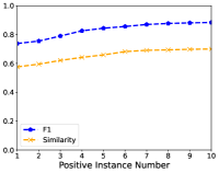
(a)

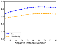
(b)

Figure 5. The Impact of Positive and Negative Instance Number on F1 and Similarity

7.6. Ablation Study

7.6.1. Effectiveness of Demonstration Example Compression Strategy

In this experiment, we investigate the impact of the proposed demonstration example compression strategy on the performance of ICLCR. In particular, we compare the standard ICLCR against ICLCR-DEC, a version of ICLCR that does not include the demonstration example compression strategy to increase the maximum number of demonstration examples $k_{max}$ for the prompt input. As shown in Table 12, ICLCR outperforms ICLCR-DEC, with a relative improvement of 3.47% and 3.89% on Real and Join, respectively, which demonstrates the effectiveness of the proposed demonstration example compression strategy.

Table 12. Impact of the demonstration compression strategy on multi-tuple conflict resolution

	Overall	Small	Medium	Large	Overall	Small	Medium	Large
ICLCR-DEC	0.691	0.698	0.690	0.711	0.712	0.697	0.707	0.719
ICLCR	0.736	0.742	0.729	0.754	0.757	0.745	0.754	0.761

7.6.2. Impact of Demonstration Example Selection Strategies

We also compare three different demonstration example selection strategies, Random, $k$-NN, and weighted $k$-NN in ICLCR to investigate the impact on model performance. As shown in Table 13, we can first observe that random selection of demonstration examples does not fully exploit the performance of ICLCR. This is shown by ICLCR performing worse with a random selection strategy, compared to the two $k$-NN strategies, which demonstrates the importance of selecting relevant demonstration examples to instruct the LLM for prediction in ICLCR. Furthermore, ICLCR with the weighted $k$-NN selection strategy achieves the highest Accuracy in every case. On average, ICLCR with the weighted $k$-NN selection strategy outperforms ICLCR with $k$-NN selection strategy by 1.52% and 1.45% on Real and Join, respectively. This is because the weighted $k$-NN selection strategy considers the importance of different attributes for a target attribute.

Table 13. The impact of the demonstration selection strategies on multi-tuple conflict resolution

Methods	Real				Join
	Overall	Small	Medium	Large	Overall	Small	Medium	Large
Random	0.714	0.723	0.713	0.737	0.739	0.723	0.734	0.742
$k$-NN	0.725	0.734	0.720	0.744	0.746	0.737	0.745	0.751
Weighted $k$-NN	0.736	0.742	0.729	0.754	0.757	0.745	0.754	0.761

7.6.3. Pairwise integrability judgment

Overall, it takes SSACL and Unicorn 103ms and 126ms to judge the integrability for each tuple pair on average. The average inference time of the two methods are similar, since both of them rely on a pre-trained large language model to construct the tuple representations and make prediction.

7.6.4. Integrable set discovery

In this experiment, we conduct an efficiency study to compare the time costs of various methods on integrable set discovery. Table 14 shows the running time cost for these methods using the J11 dataset. Observe that the GNN incurs the highest time costs due to the computationally intensive aggregation operations used. Considering that GNN delivers optimal performance for integrable set discovery and the time required for integrable set discovery is significantly less than pairwise integrability judgment, GNNs are still the preferred choice for integrable set discovery.

Table 14. The efficiency of different integrable set discovery methods on R11 dataset

Methods	Time (Hours)
BK	3.41
Louvain	2.62
GN	3.37
SC	3.64
Infomap	2.35
GNN	3.91

7.6.5. Multi-tuple conflict resolution

On average, it takes ICLCR and SlimFast 35ms and 157ms to make predictions for each integrable set in the dataset $J11$. Our approach is more costly for two reasons: (1) ICLCR relies on an LLM to make the predictions, which has higher model complexity than SlimFast; (2) Our model is based on in-context learning, which requires the model to input each text test case as well as any demonstration examples. Thus, a larger input size has higher running time costs. However, considering that the relative performance improvement for ICLCR over SlimFast is high, the additional time cost is an acceptable trade-off.

7.7. Additional Experiment on The Task of Entity Resolution

As discussed in Sec. 8, despite challenges encountered, such as representative noise and missing values, entity resolution and pairwise integrability judgment share similar goals. Hence, we conduct an additional experiment to compare the proposed SSACL with state-of-the-art ER methods on the entity resolution problem, using five widely used ER datasets: DBLP-Scholar (DS), DBLP-ACM (DA), Walmart-Amazon (WA), Amazon-Goolge (AG), and Itunes-Amazon (IA). Since the original ER datasets are error-free, we create two modified versions of the datasets for each original ER dataset: (1) We apply the noise injection method introduced in Sec. 6.1 to create the new versions of the ER dataset; (2) Following (Mudgal et al., 2018), the “imperfect” datasets are generated by randomly emptying attributes and appending their values to other randomly selected attributes. We compare our proposed SSACL against both Unicorn (a state-of-the-art supervised method) and sudowoodo (Wang et al., 2023) (a state-of-the-art unsupervised method).

Table 15,  16, and  17 show the F1 Scores for all of the methods using the three different variants of the ER datasets, respectively. Observe that: (1) Unicorn undoubtedly achieves the best performance, since it is the only method that is trained using high-quality labeled data. However, its performance drops sharply on the “imperfect” datasets when compared against SSACL. Specifically, Unicorn exhibits an average performance decrease of $10.0\%$ and $6.6\%$ when shifting from complete datasets to imperefect datasets containing typographical errors, semantic equivalence, and attribute replacement, respectively, while the average performance decreases for SSACL is $3.7\%$ and $1.1\%$, respectively. (2) On imperfect datasets with typographical errors and semantic equivalence, our method SSACL outperforms Sudowoodo, with an average improvement of $2.03\%$. (3) On imperfect datasets with the attribute replacement, SSACL achieves a comparable performance with that of Sudowoodo. (3) Even on the complete datasets, the performance of SSACL is similar to Sudowoodo.

In summary, our SSACL is robust to noisy data, while maintaining a promising performance on complete data for the entity resolution task.

Table 15. Relative performance of five ER datasets containing typographical errors and semantic equivalence using F1.

	Sudowoodo	Unicorn	SSACL
DS	76.3	83.4	78.2
WA	64.1	71.8	65.6
DA	86.4	89.0	87.4
AG	59.7	64.0	61.2
IA	82.7	90.3	85.4

Table 16. Relative performance of five ER datasets with attribute replacement using F1.

	Sudowoodo	Unicorn	Ours
DS	81.8	87.7	80.3
WA	68.1	75.4	67.2
DA	90.3	92.3	91.7
AG	63.7	67.2	64.1
IA	83.2	90.3	84.4

Table 17. Relative performance using five ER datasets using F1.

	Sudowoodo	Unicorn	Ours
DS	84.7	93.1	82.5
WA	71.6	82.9	68.4
DA	93.8	98.5	92.9
AG	65.4	70.4	63.2
IA	87.3	97.6	85.6

8. Related Work

Entity Resolution.  The most relevant work for pairwise integrability judgment is entity resolution, which determines whether two entities refer to the same entity. Existing methods can be divided into four categories: rule-based methods (Fan et al., 2009; Singh et al., 2017a, b), crowdsourcing methods (Chai et al., 2016, 2018; Fan et al., 2015; Cui et al., 2021; Yang et al., 2018), conventional machine learning (ML)-based methods (Bilenko and Mooney, 2003; Tejada et al., 2002; McCallum and Wellner, 2004), and deep learning (DL)-based methods (Ebraheem et al., 2018; Li et al., 2020; Mudgal et al., 2018; Tu et al., 2022, 2023; Li et al., 2023; Yao et al., 2022; Wang et al., 2023; Wu et al., 2020; Thirumuruganathan et al., 2021).

Currently, DL-based methods are considered state-of-the-art and often demonstrate the best overall performance. In particular, DeepER (Ebraheem et al., 2018) uses Long Short-Term Memory (LSTM), a type of recurrent neural network, to learn tuple representations using pre-trained word embeddings such as GloVe (Pennington et al., 2014). Then, a multi-layer perceptron (MLP) is used to evaluate the similarity between the two tuple representations. DeepMatcher (Mudgal et al., 2018) categorizes ER problems into three types – structured ER, textual ER, and “dirty” ER – and provides a comprehensive and systematic solution designs for each. Ditto (Li et al., 2020) leverages domain knowledge and data augmentation, to futher enhance the performance of entity resolution. EMBDI (Cappuzzo et al., 2020) represents the relational database as a compact graph and learns local embeddings that are effective for data integration tasks including entity resolution. DADER (Tu et al., 2022) systematically investigates the problem of domain adaption for entity resolution, addressing scenarios where an ER model trained from a source dataset is applied to a target dataset using little or no labeled data. HierGAT uses contextual embeddings to learn more accurate tuple representations, and then employs a hierarchical graph attention transformer network to automatically identify the most discriminative words and attributes in a tuple. Unicorn (Tu et al., 2023) introduces a unified framework for entity resolution and five other data matching tasks, and also proposes a multi-task learning framework that enables task performance to be improved holistically.

Apart from these supervised ER methods which require high-quality labeled data to train the models, there is also work that investigates how to train an effective machine learning model using limited labeled data in an unsupervised manner. ZeroER (Wu et al., 2020) tackles Entity Resolution without labeled examples, matching the performance of supervised methods by using Gaussian Mixture Models and adaptive regularization. It also incorporates transitivity into its generative model, enhancing accuracy on benchmark ER datasets. Sudowoodo (Wang et al., 2023) is a versatile data integration and preparation framework using contrastive representation learning to perform tasks like entity resolution and error correction without labeled data. It learns similarity-aware data representations, which can be fine-tuned with minimal labels, achieving state-of-the-art results across various data integration and preparation tasks.

While entity resolution is similar to pairwise integrability judgment, there are several important distinctions: (1) As introduced in Sec. 2, pairwise integrability judgment represents a broader concept than entity resolution, since two tuples that do not refer to the same entity can still be integrable. (2) Pairwise integrability judgment matches tuples containing representative noise, which include issues such as typographical errors and semantic equivalence. (3) Entities in entity resolution are typically derived from comprehensive information, whereas the tuples in our task usually involve missing values – a common occurrence in large data lakes, especially when using an outer union operator. This disparity demands a different type of comparison at the attribute-level for two tuples, as opposed to a tuple-level assessment based on prior knowledge.

Data Fusion.  Data fusion (Meng et al., 2020; Bleiholder and Naumann, 2009; Azzalini et al., 2023) determines how to merge multiple tuples, which map to the same entity but originate from other resources, into a unified and comprehensive representation. At the core of data fusion lies the challenge of addressing conflicts when multiple values exist for a particular attribute. Although a few simple, yet intuitive methods, such as using the mean or median values for numerical values or using majority voting for categorical data can be employed, they often reduce the quality of the data produced.

Existing solutions (Rekatsinas et al., 2017; Broelemann et al., 2017; Xiao et al., 2016; Li et al., 2014) for data fusion predominantly rely on the concept of truth discovery, which involves assessing the reliability of each data source and selecting the value using the most reliable source. Generally speaking, those methods can be categorized into three groups: probability-based methods (Zhang et al., 2016; Fang, 2017; Lin and Chen, 2018), optimization-based methods (Wang et al., 2017; Li et al., 2016), and machine learning (ML)-based methods (Xiao et al., 2016; Broelemann et al., 2017; Rekatsinas et al., 2017). Among all the methods, ML-based truth discovery methods achieve the best performance. Specifically, LTD-RBM (Broelemann et al., 2017) proposes a novel truth discovery methods based on Restricted Boltzmann Machine (RBM), which is able to handle both continuous and discret values. LTD-RBM also provides an effective and robust inference procedure based on Contrastive Divergence and Gibbs Sampling. ETCIBoot (Xiao et al., 2016) enhances traditional truth discovery techniques by providing confidence intervals alongside truth estimates, offering a measure of certainty. ETCIBoot involves updating source weights, estimating truths, and constructing confidence intervals using bootstrapping. This approach is particularly beneficial in scenarios with varying data density, ensuring more reliable and informative truth discovery. SLiMFast (Rekatsinas et al., 2017) frames Data Fusion as a statistical learning problem using discriminative probabilistic models. It includes components for compilation, optimization, and data fusion, focusing on estimating data source accuracy and predicting true values through statistical learning and probabilistic inference. Uniquely, SLiMFast combines cross-source conflicts with domain-specific features to improve source accuracy estimation.

However, estimating source reliability for truth discovery methods heavily depends on labeled data, metadata (such as paper citations and webpage views), or domain knowledge. Unfortunately, such data is usually scarce in data lakes, which motivates us to develop an effective conflict resolution method even with limited labeled data.

8.1. Large Language Models.

Large Language Models (LLMs) (He et al., 2020; Devlin et al., 2019; Touvron et al., 2023) are advanced machine learning models designed to understand and generate human language. They are built on deep neural networks such as Transformers (Vaswani et al., 2017), and are trained on vast amounts of text data. Due to their success in textual data, there is a growing interest in applying LLMs to tabular data. Specifically, there are two primary approaches to leveraging LLMs for tasks involving tabular data.

The first approach involves using LLMs to learn semantic and comprehensive representations for tabular data. Depending on the characteristics of the downstream tasks, these representations are learned at different levels, such as row-level, column-level, and table-level. For example, recent work on entity resolution, such as Ditto (Li et al., 2020) and Unicorn (Tu et al., 2023), applies LLMs to learn row-level representations. In contrast, recent column annotation methods, such as DuDuo (Suhara et al., 2022), typically utilize LLMs to learn column-level representations. Furthermore, for dataset discovery tasks (Fan et al., 2023b), LLMs are often employed to learn representations for entire tables to find similar tables. The second approach involves utilizing LLMs as decision models. In this case, LLMs are not part of the encoding process but are instead used to make final decisions. The downstream task is first transformed into a natural language query, which the LLM then answers. For example, RPT (Tang et al., 2021) uses a generative large language model to address various data preparation tasks, such as error correction, data transformation, and data annotation.

Both techniques are employed in this work. Specifically, like most entity resolution work, SSACL uses LLMs to learn tuple representations, while ICLCR uses LLMs to make final predictions for the conflict resolution task.

9. Conclusion

In this paper, we solve three core tasks for data integration in data lake tables, pairwise integrability judgment, integrable set discovery, and multi-tuple conflict resolution. To solve the task pairwise integrability judgment, we develop a binary classifier, which is able to determine whether any two tuples should be integrated even when they are semantically equivalent, or contain typographical errors. Then we cast the problem of integrable set discovery to finding maximal cliques or densely connected subgraphs, i.e., communities, in a graph, and explore a collection of representative algorithms to solve it. For the task multi-tuple conflict resolution, we propose a novel in-context learning (ICL)-based algorithm, which enables us to leverage the extensive knowledge embedded in pretrained large language models to make predictions. Finally, our methods show promising performance improvements using limited labeled data.

References

- (1)
- Abedjan et al. (2016) Ziawasch Abedjan, Xu Chu, Dong Deng, Raul Castro Fernandez, Ihab F Ilyas, Mourad Ouzzani, Paolo Papotti, Michael Stonebraker, and Nan Tang. 2016. Detecting data errors: Where are we and what needs to be done? VLDB 2016 9, 12 (2016), 993–1004.
- Akyürek et al. (2022) Ekin Akyürek, Dale Schuurmans, Jacob Andreas, Tengyu Ma, and Denny Zhou. 2022. What learning algorithm is in-context learning? Investigations with linear models. In ICLR 2022.
- Armandpour et al. (2019) Mohammadreza Armandpour, Patrick Ding, Jianhua Huang, and Xia Hu. 2019. Robust negative sampling for network embedding. In AAAI 2019, Vol. 33. 3191–3198.
- Awasthi et al. (2022) Pranjal Awasthi, Nishanth Dikkala, and Pritish Kamath. 2022. Do more negative samples necessarily hurt in contrastive learning?. In ICML 2022. PMLR, 1101–1116.
- Azzalini et al. (2023) Fabio Azzalini, Davide Piantella, Emanuele Rabosio, and Letizia Tanca. 2023. Enhancing domain-aware multi-truth data fusion using copy-based source authority and value similarity. The VLDB Journal 32, 3 (2023), 475–500.
- Bayer et al. (2022) Markus Bayer, Marc-André Kaufhold, and Christian Reuter. 2022. A survey on data augmentation for text classification. Comput. Surveys 55, 7 (2022), 1–39.
- Bilenko and Mooney (2003) Mikhail Bilenko and Raymond J Mooney. 2003. Adaptive duplicate detection using learnable string similarity measures. In SIGKDD 2003. 39–48.
- Bleiholder and Naumann (2009) Jens Bleiholder and Felix Naumann. 2009. Data fusion. ACM computing surveys (CSUR) 41, 1 (2009), 1–41.
- Bleiholder et al. (2010) Jens Bleiholder, Sascha Szott, Melanie Herschel, Frank Kaufer, and Felix Naumann. 2010. Subsumption and complementation as data fusion operators. In EDBT 2010. 513–524.
- Blondel et al. (2008) Vincent D Blondel, Jean-Loup Guillaume, Renaud Lambiotte, and Etienne Lefebvre. 2008. Fast unfolding of communities in large networks. Journal of statistical mechanics: theory and experiment 2008, 10 (2008), P10008.
- Bojanowski et al. (2017) Piotr Bojanowski, Edouard Grave, Armand Joulin, and Tomas Mikolov. 2017. Enriching word vectors with subword information. TACL 5 (2017), 135–146.
- Boyd and Vandenberghe (2004) Stephen Boyd and Lieven Vandenberghe. 2004. Convex Optimization. Cambridge University Press, Cambridge, UK.
- Broelemann et al. (2017) Klaus Broelemann, Thomas Gottron, and Gjergji Kasneci. 2017. LTD-RBM: Robust and fast latent truth discovery using restricted Boltzmann machines. In ICDE 2017. IEEE, 143–146.
- Brown et al. (2020) Tom Brown, Benjamin Mann, Nick Ryder, Melanie Subbiah, Jared D Kaplan, Prafulla Dhariwal, Arvind Neelakantan, Pranav Shyam, Girish Sastry, Amanda Askell, et al. 2020. Language models are few-shot learners. NIPS 2020 33 (2020), 1877–1901.
- Bruna and Li (2017) Joan Bruna and X Li. 2017. Community detection with graph neural networks. stat 1050 (2017), 27.
- Cappuzzo et al. (2020) Riccardo Cappuzzo, Paolo Papotti, and Saravanan Thirumuruganathan. 2020. Creating embeddings of heterogeneous relational datasets for data integration tasks. In SIGMOD 2020. 1335–1349.
- Chai et al. (2016) Chengliang Chai, Guoliang Li, Jian Li, Dong Deng, and Jianhua Feng. 2016. Cost-effective crowdsourced entity resolution: A partial-order approach. In SIGMOD 2016. 969–984.
- Chai et al. (2018) Chengliang Chai, Guoliang Li, Jian Li, Dong Deng, and Jianhua Feng. 2018. A partial-order-based framework for cost-effective crowdsourced entity resolution. The VLDB Journal 27 (2018), 745–770.
- Cui et al. (2021) Lizhen Cui, Jing Chen, Wei He, Hui Li, Wei Guo, and Zhiyuan Su. 2021. Achieving approximate global optimization of truth inference for crowdsourcing microtasks. Data Science and Engineering 6, 3 (2021), 294–309.
- Devlin et al. (2019) Jacob Devlin, Ming-Wei Chang, Kenton Lee, and Kristina Toutanova. 2019. BERT: Pre-training of Deep Bidirectional Transformers for Language Understanding. In NAACL 2019. 4171–4186. https://doi.org/10.18653/v1/N19-1423
- Dong and Naumann (2009) Xin Luna Dong and Felix Naumann. 2009. Data fusion: resolving data conflicts for integration. VLDB 2009 2, 2 (2009), 1654–1655.
- Ebraheem et al. (2018) Muhammad Ebraheem, Saravanan Thirumuruganathan, Shafiq Joty, Mourad Ouzzani, and Nan Tang. 2018. Distributed representations of tuples for entity resolution. VLDB 2018 11, 11 (2018), 1454–1467.
- Edunov et al. (2018) Sergey Edunov, Myle Ott, Michael Auli, and David Grangier. 2018. Understanding Back-Translation at Scale. In EMNLP 2018. 489–500.
- Fan et al. (2023a) Grace Fan, Jin Wang, Yuliang Li, and Renée J Miller. 2023a. Table Discovery in Data Lakes: State-of-the-art and Future Directions. In Companion of the 2023 International Conference on Management of Data. 69–75.
- Fan et al. (2023b) Grace Fan, Jin Wang, Yuliang Li, Dan Zhang, and Renée J Miller. 2023b. Semantics-Aware Dataset Discovery from Data Lakes with Contextualized Column-Based Representation Learning. VLDB 2023 16, 7 (2023), 1726–1739.
- Fan et al. (2015) Ju Fan, Guoliang Li, Beng Chin Ooi, Kian-lee Tan, and Jianhua Feng. 2015. icrowd: An adaptive crowdsourcing framework. In SIGMOD 2015. 1015–1030.
- Fan et al. (2009) Wenfei Fan, Xibei Jia, Jianzhong Li, and Shuai Ma. 2009. Reasoning about record matching rules. VLDB 2009 2, 1 (2009), 407–418.
- Fang (2017) Xiu Susie Fang. 2017. Truth discovery from conflicting multi-valued objects. In WWW 2017 Companion. 711–715.
- Feng et al. (2021) Steven Y Feng, Varun Gangal, Jason Wei, Sarath Chandar, Soroush Vosoughi, Teruko Mitamura, and Eduard Hovy. 2021. A Survey of Data Augmentation Approaches for NLP. In Findings of the Association for Computational Linguistics: ACL-IJCNLP 2021. 968–988.
- Goodfellow et al. (2014) Ian J Goodfellow, Jonathon Shlens, and Christian Szegedy. 2014. Explaining and harnessing adversarial examples. arXiv preprint arXiv:1412.6572 (2014).
- Hai et al. (2016) Rihan Hai, Sandra Geisler, and Christoph Quix. 2016. Constance: An intelligent data lake system. In SIGMOD 2016. 2097–2100.
- He et al. (2020) Pengcheng He, Xiaodong Liu, Jianfeng Gao, and Weizhu Chen. 2020. DeBERTa: Decoding-enhanced BERT with Disentangled Attention. arXiv preprint arXiv:2006.03654 (2020).
- Ilyas et al. (2019) Andrew Ilyas, Shibani Santurkar, Dimitris Tsipras, Logan Engstrom, Brandon Tran, and Aleksander Madry. 2019. Adversarial examples are not bugs, they are features. NIPS 2019 32 (2019).
- Kenton and Toutanova (2019) Jacob Devlin Ming-Wei Chang Kenton and Lee Kristina Toutanova. 2019. BERT: Pre-training of Deep Bidirectional Transformers for Language Understanding. In NAACL 2019. 4171–4186.
- Khatiwada et al. (2023) Aamod Khatiwada, Grace Fan, Roee Shraga, Zixuan Chen, Wolfgang Gatterbauer, Renée J Miller, and Mirek Riedewald. 2023. SANTOS: Relationship-based Semantic Table Union Search. SIGMOD 2023 1, 1 (2023), 1–25.
- Khatiwada et al. (2022) Aamod Khatiwada, Roee Shraga, Wolfgang Gatterbauer, and Renée J Miller. 2022. Integrating Data Lake Tables. VLDB 2022 16, 4 (2022), 932–945.
- Khosla et al. (2020) Prannay Khosla, Piotr Teterwak, Chen Wang, Aaron Sarna, Yonglong Tian, Phillip Isola, Aaron Maschinot, Ce Liu, and Dilip Krishnan. 2020. Supervised contrastive learning. NIPS 2020 33 (2020), 18661–18673.
- Kingma (2014) DP Kingma. 2014. Adam: a method for stochastic optimization. In ICLR 2014.
- Li et al. (2014) Qi Li, Yaliang Li, Jing Gao, Lu Su, Bo Zhao, Murat Demirbas, Wei Fan, and Jiawei Han. 2014. A confidence-aware approach for truth discovery on long-tail data. VLDB 2015 8, 4 (2014), 425–436.
- Li et al. (2012) Xian Li, Xin Luna Dong, Kenneth Lyons, Weiyi Meng, and Divesh Srivastava. 2012. Truth Finding on the Deep Web: Is the Problem Solved? VLDB 2013 6, 2 (2012).
- Li et al. (2020) Yuliang Li, Jinfeng Li, Yoshihiko Suhara, AnHai Doan, and Wang-Chiew Tan. 2020. Deep entity matching with pre-trained language models. VLDB 2021 14, 1 (2020), 50–60.
- Li et al. (2023) Yuliang Li, Jinfeng Li, Yoshi Suhara, AnHai Doan, and Wang-Chiew Tan. 2023. Effective entity matching with transformers. The VLDB Journal (2023), 1–21.
- Li et al. (2016) Yaliang Li, Qi Li, Jing Gao, Lu Su, Bo Zhao, Wei Fan, and Jiawei Han. 2016. Conflicts to harmony: A framework for resolving conflicts in heterogeneous data by truth discovery. TKDE 28, 8 (2016), 1986–1999.
- Lin and Chen (2018) Xueling Lin and Lei Chen. 2018. Domain-aware multi-truth discovery from conflicting sources. VLDB 2018 11, 5 (2018), 635–647.
- Liu et al. (2019) Yinhan Liu, Myle Ott, Naman Goyal, Jingfei Du, Mandar Joshi, Danqi Chen, Omer Levy, Mike Lewis, Luke Zettlemoyer, and Veselin Stoyanov. 2019. RoBERTa: A Robustly Optimized BERT Pretraining Approach. arXiv preprint arXiv:1907.11692 (2019).
- McCallum and Wellner (2004) Andrew McCallum and Ben Wellner. 2004. Conditional models of identity uncertainty with application to noun coreference. NIPS 2004 17 (2004).
- Meng et al. (2020) Tong Meng, Xuyang Jing, Zheng Yan, and Witold Pedrycz. 2020. A survey on machine learning for data fusion. Information Fusion 57 (2020), 115–129.
- Mikolov et al. (2013) Tomas Mikolov, Ilya Sutskever, Kai Chen, Greg S Corrado, and Jeff Dean. 2013. Distributed representations of words and phrases and their compositionality. NIPS 2013 26 (2013).
- Miller (1995) George A Miller. 1995. WordNet: a lexical database for English. Commun. ACM 38, 11 (1995), 39–41.
- Min et al. (2022) Sewon Min, Xinxi Lyu, Ari Holtzman, Mikel Artetxe, Mike Lewis, Hannaneh Hajishirzi, and Luke Zettlemoyer. 2022. Rethinking the Role of Demonstrations: What Makes In-Context Learning Work?. In EMNLP 2022. 11048–11064.
- Mudgal et al. (2018) Sidharth Mudgal, Han Li, Theodoros Rekatsinas, AnHai Doan, Youngchoon Park, Ganesh Krishnan, Rohit Deep, Esteban Arcaute, and Vijay Raghavendra. 2018. Deep learning for entity matching: A design space exploration. In SIGMOD 2018. 19–34.
- Nargesian et al. (2019) Fatemeh Nargesian, Erkang Zhu, Renée J Miller, Ken Q Pu, and Patricia C Arocena. 2019. Data lake management: challenges and opportunities. VLDB 2019 12, 12 (2019), 1986–1989.
- Nargesian et al. (2018) Fatemeh Nargesian, Erkang Zhu, Ken Q Pu, and Renée J Miller. 2018. Table union search on open data. VLDB 2018 11, 7 (2018), 813–825.
- Newman (2013) Mark EJ Newman. 2013. Spectral methods for community detection and graph partitioning. Physical Review E 88, 4 (2013), 042822.
- Newman and Girvan (2004) M. E. J. Newman and M. Girvan. 2004. Finding and evaluating community structure in networks. Physical Review E 69, 2 (2004), 026113.
- Ng et al. (2001) Andrew Y. Ng, Michael I. Jordan, and Yair Weiss. 2001. On spectral clustering: Analysis and an algorithm. In NIPS 2001. 849–856.
- Nocedal and Wright (2006) Jorge Nocedal and Stephen J. Wright. 2006. Numerical Optimization (2e ed.). Springer, New York, NY, USA.
- Peng et al. (2022) Jinfeng Peng, Derong Shen, Nan Tang, Tieying Liu, Yue Kou, Tiezheng Nie, Hang Cui, and Ge Yu. 2022. Self-supervised and Interpretable Data Cleaning with Sequence Generative Adversarial Networks. VLDB 2023 16, 3 (2022), 433–446.
- Pennington et al. (2014) Jeffrey Pennington, Richard Socher, and Christopher D Manning. 2014. Glove: Global vectors for word representation. In EMNLP 2014. 1532–1543.
- Raffel et al. (2020) Colin Raffel, Noam Shazeer, Adam Roberts, Katherine Lee, Sharan Narang, Michael Matena, Yanqi Zhou, Wei Li, and Peter J Liu. 2020. Exploring the limits of transfer learning with a unified text-to-text transformer. JMLR 21, 1 (2020), 5485–5551.
- Regneri (2007) Michaela Regneri. 2007. Finding all cliques of an undirected graph. In Seminar current trends in IE WS jun.
- Rekatsinas et al. (2017) Theodoros Rekatsinas, Manas Joglekar, Hector Garcia-Molina, Aditya Parameswaran, and Christopher Ré. 2017. Slimfast: Guaranteed results for data fusion and source reliability. In SIGMOD 2017. 1399–1414.
- Rosvall and Bergstrom (2008) Martin Rosvall and Carl T Bergstrom. 2008. Maps of random walks on complex networks reveal community structure. Proceedings of the National Academy of Sciences 105, 4 (2008), 1118–1123.
- Sanh et al. (2019) Victor Sanh, Lysandre Debut, Julien Chaumond, and Thomas Wolf. 2019. DistilBERT, a distilled version of BERT: smaller, faster, cheaper and lighter. arXiv preprint arXiv:1910.01108 (2019).
- Shorten et al. (2021) Connor Shorten, Taghi M Khoshgoftaar, and Borko Furht. 2021. Text data augmentation for deep learning. Journal of big Data 8 (2021), 1–34.
- Singh et al. (2017a) Rohit Singh, Vamsi Meduri, Ahmed Elmagarmid, Samuel Madden, Paolo Papotti, Jorge-Arnulfo Quiané-Ruiz, Armando Solar-Lezama, and Nan Tang. 2017a. Generating concise entity matching rules. In SIGMOD 2017. 1635–1638.
- Singh et al. (2017b) Rohit Singh, Venkata Vamsikrishna Meduri, Ahmed Elmagarmid, Samuel Madden, Paolo Papotti, Jorge-Arnulfo Quiané-Ruiz, Armando Solar-Lezama, and Nan Tang. 2017b. Synthesizing entity matching rules by examples. VLDB 2018 11, 2 (2017), 189–202.
- Suhara et al. (2022) Yoshihiko Suhara, Jinfeng Li, Yuliang Li, Dan Zhang, Çağatay Demiralp, Chen Chen, and Wang-Chiew Tan. 2022. Annotating columns with pre-trained language models. In SIGMOD 2022. 1493–1503.
- Tang et al. (2021) Nan Tang, Ju Fan, Fangyi Li, Jianhong Tu, Xiaoyong Du, Guoliang Li, Sam Madden, and Mourad Ouzzani. 2021. RPT: relational pre-trained transformer is almost all you need towards democratizing data preparation. VLDB 2021 14, 8 (2021), 1254–1261.
- Tejada et al. (2002) Sheila Tejada, Craig A Knoblock, and Steven Minton. 2002. Learning domain-independent string transformation weights for high accuracy object identification. In SIGKDD 2002. 350–359.
- Thirumuruganathan et al. (2021) Saravanan Thirumuruganathan, Han Li, Nan Tang, Mourad Ouzzani, Yash Govind, Derek Paulsen, Glenn Fung, and AnHai Doan. 2021. Deep learning for blocking in entity matching: a design space exploration. VLDB 2021 14, 11 (2021), 2459–2472.
- Touvron et al. (2023) Hugo Touvron, Thibaut Lavril, Gautier Izacard, Xavier Martinet, Marie-Anne Lachaux, Timothée Lacroix, Baptiste Rozière, Naman Goyal, Eric Hambro, Faisal Azhar, et al. 2023. Llama: Open and efficient foundation language models. arXiv preprint arXiv:2302.13971 (2023).
- Tu et al. (2022) Jianhong Tu, Ju Fan, Nan Tang, Peng Wang, Chengliang Chai, Guoliang Li, Ruixue Fan, and Xiaoyong Du. 2022. Domain adaptation for deep entity resolution. In SIGMOD 2022. 443–457.
- Tu et al. (2023) Jianhong Tu, Ju Fan, Nan Tang, Peng Wang, Guoliang Li, Xiaoyong Du, Xiaofeng Jia, and Song Gao. 2023. Unicorn: A unified multi-tasking model for supporting matching tasks in data integration. SIGMOD 2023 1, 1 (2023), 1–26.
- Vaswani et al. (2017) Ashish Vaswani, Noam Shazeer, Niki Parmar, Jakob Uszkoreit, Llion Jones, Aidan N Gomez, Łukasz Kaiser, and Illia Polosukhin. 2017. Attention is all you need. NIPS 2017 30 (2017).
- Wang et al. (2023) Runhui Wang, Yuliang Li, and Jin Wang. 2023. Sudowoodo: Contrastive self-supervised learning for multi-purpose data integration and preparation. In ICDE 2023. IEEE, 1502–1515.
- Wang et al. (2017) Yaqing Wang, Fenglong Ma, Lu Su, and Jing Gao. 2017. Discovering truths from distributed data. In ICDM 2017. IEEE, 505–514.
- Wu et al. (2020) Renzhi Wu, Sanya Chaba, Saurabh Sawlani, Xu Chu, and Saravanan Thirumuruganathan. 2020. Zeroer: Entity resolution using zero labeled examples. In SIGMOD 2020. 1149–1164.
- Xiao et al. (2016) Houping Xiao, Jing Gao, Qi Li, Fenglong Ma, Lu Su, Yunlong Feng, and Aidong Zhang. 2016. Towards confidence in the truth: A bootstrapping based truth discovery approach. In SIGKDD 2016. 1935–1944.
- Xie et al. (2021) Sang Michael Xie, Aditi Raghunathan, Percy Liang, and Tengyu Ma. 2021. An Explanation of In-context Learning as Implicit Bayesian Inference. In ICLR 2021.
- Yang et al. (2018) Jingru Yang, Ju Fan, Zhewei Wei, Guoliang Li, Tongyu Liu, and Xiaoyong Du. 2018. Cost-effective data annotation using game-based crowdsourcing. VLDB 2018 12, 1 (2018), 57–70.
- Yang et al. (2019) Zhilin Yang, Zihang Dai, Yiming Yang, Jaime Carbonell, Ruslan Salakhutdinov, and Quoc V. Le. 2019. XLNet: Generalized Autoregressive Pretraining for Language Understanding. In NIPS 2019. 5753–5763. https://doi.org/10.48550/arXiv.1906.08237
- Yao et al. (2022) Dezhong Yao, Yuhong Gu, Gao Cong, Hai Jin, and Xinqiao Lv. 2022. Entity resolution with hierarchical graph attention networks. In SIGMOD 2022. 429–442.
- Zhang et al. (2016) Hengtong Zhang, Qi Li, Fenglong Ma, Houping Xiao, Yaliang Li, Jing Gao, and Lu Su. 2016. Influence-aware truth discovery. In CIKM 2016. 851–860.
- Zhang and Li (2019) Jiliang Zhang and Chen Li. 2019. Adversarial examples: Opportunities and challenges. TNNLS 31, 7 (2019), 2578–2593.
- Zhi et al. (2015) Shi Zhi, Bo Zhao, Wenzhu Tong, Jing Gao, Dian Yu, Heng Ji, and Jiawei Han. 2015. Modeling truth existence in truth discovery. In SIGMOD 2015. 1543–1552.
- Zhu et al. (2019) Erkang Zhu, Dong Deng, Fatemeh Nargesian, and Renée J Miller. 2019. Josie: Overlap set similarity search for finding joinable tables in data lakes. In SIGMOD 2019. 847–864.