Joint Coverage and Electromagnetic Field Exposure Analysis in Downlink and Uplink for RIS-assisted Networks

Abstract

RIS have shown the potential to improve signal-to-interference-plus-noise ratio (SINR) related coverage, especially at high-frequency communications. However, assessing electromagnetic filed exposure (EMFE) and establishing EMFE regulations in RIS-assisted large-scale networks are still open issues. This paper proposes a framework to characterize SINR and EMFE in such networks for downlink and uplink scenarios. Particularly, we carefully consider the association rule with the presence of RISs, accurate antenna pattern at base stations (BSs), fading model, and power control mechanism at mobile devices in the system model. Under the proposed framework, we derive the marginal and joint distributions of SINR and EMFE in downlink and uplink, respectively. The first moment of EMFE is also provided. Additionally, we design the compliance distance (CD) between a BS/RIS and a user to comply with the EMFE regulations. To facilitate efficient identification, we further provide approximate closed-form expressions for CDs. From numerical results of the marginal distributions, we find that in the downlink scenario, deploying RISs may not always be beneficial, as the improved SINR comes at the cost of increased EMFE. However, in the uplink scenario, RIS deployment is promising to enhance coverage while still maintaining EMFE compliance. By simultaneously evaluating coverage and compliance metrics through joint distributions, we demonstrate the feasibility of RISs in improving uplink and downlink performance. Insights from this framework can contribute to establishing EMFE guidelines and achieving a balance between coverage and compliance when deploying RISs.

I Introduction

Radio frequency (RF) radiation emitted by base stations (in downlink) and mobile devices (in uplink) generates EMFE in cellular networks. If not controlled, EMFE can have potential adverse thermal effects on exposed tissues, endangering population health. Regulatory authorities (e.g., International Commission on Non-Ionizing Radiation Protection (ICNIRP) [2] and Federal Communications Commission (FCC) [3]) have implemented regulations to ensure EMFE within a safe limit in current cellular networks. This includes the establishment of the CD between a BS and a user. If a user enters an area centered at a BS with a radius of the CD, the corresponding EMFE may exceed the safe limit and user safety cannot be guaranteed. Hence, the assessment of EMFE and the establishment of EMFE regulations are crucial in developing future cellular networks [4].

A novel technology, reconfigurable intelligent surface (RIS), consisting of numerous passive elements, can reflect incident waves into specific directions by dynamically adjusting the element phases [5]. This enables RISs to establish a cascaded line-of-light (LoS) link between a BS and a user and provide directional transmission gain (i.e., RIS gain), effectively alleviating blockage effects and compensating path loss. Hence, RISs hold significant promise for extending coverage of future cellular networks, especially at high-frequency communizations [6]. The potential impact of RISs on EMFE has also attracted great attention. Under the constraints of EMFE, researchers optimized the BS beamforming and/or RIS phases to maximize the SINR or capacity in a single cell with a RIS [7, 8] or multiple RISs [9]. On the other hand, under the constraints of SINR, spectral efficiency, or throughput, researchers designed RIS phases to minimize uplink and/or downlink exposure in a single cell with a RIS [10, 11, 12] or multiple RISs [13]. The authors in [14] extended the analysis to multi-cell scenarios, where BSs and RISs are deployed at specific locations. These studies highlight the necessity of considering the impact of RISs on EMFE and underscore the importance of jointly assessing this impact alongside SINR. However, these studies either focus on small-scale analysis (neglecting EMFE and interference from neighboring cells) or fail to adequately characterize the spatial randomness of transmission nodes and obstacles, as well as the spatial characteristics of transmission links.

Comprehensive large-scale analysis on RIS-assisted multi-cell networks with spatial randomness is an unexplored yet critical research area. RISs, with the capability of concentrating the energy of incident waves into a specific direction, introduce potential EMFE risks, particularly in that concentrated direction. In this context, several crucial questions arise: Does deploying large-scale RISs exacerbate EMFE? Should a specific CD be established for a RIS? How do RISs impact network SINR and EMFE in downlink/uplink simultaneously? What deployment strategy can enhance SINR while effectively mitigating EMFE? We aim to answer these questions by providing marginal/joint distributions of downlink/uplink SINR and EMFE in large-scale RIS-assisted networks under a random spatial network model.

I-A Related Works

SG is a useful tool for modeling large-scale network topologies with randomly distributed nodes and analyzing performance metrics [15, 16]. This tool has recently been applied to model RIS-assisted cellular networks and analyze the distribution of SINR. The authors in [17] modeled the locations of RISs, BSs, and users as homogeneous Poisson point processes and modeled RIS orientations under a line Boolean model. Considering that RISs can provide cascaded LoS links when the direct link between a user and its nearest BS is non-line-of-sight (NLoS) [18, 19, 20], the statistics of cascaded links are characterized by the reflection probability of the RIS, the association probability, and the distance distributions. The authors in [21, 19, 20] derived the complementary cumulative distribution function (CCDF) of SINR of the networks consisting of BSs with uniform linear arrays and RISs. Under a practical channel state information (CSI) assumption that the channel angle information is known, a simplified but not accurate antenna model (flat-top pattern) was adopted to characterize directional transmission gain. The above works have demonstrated the feasibility of RISs in improving downlink communication quality. Additionally, considering the fixed transmit power at mobile devices, RISs can enhance uplink coverage [22].

In large-scale networks without RISs, researchers have characterized the cumulative distribution function (CDF) of EMFE using tools from stochastic geometry (SG) for omnidirectional antennas [23, 24] and directional antennas [25, 26]. Under the distance-dependent power control mechanism at the mobile devices, the authors in [23, 24] evaluated uplink EMFE. Assuming the perfect CSI (including not only angle information) for beamforming, the downlink EMFE for multi-antenna BSs was analyzed [25]. The authors in [26] analyzed the CDF of downlink EMFE (measured by received power density at the typical user) from macro-cell BSs and small-cell BSs under a flat-top/sectored antenna patterns based on the channel angle information. Moreover, the BS CD (i.e., the minimum allowable separation between a BS and a user which ensures that the corresponding EMFE must not exceed the maximum allowable limit with a predefined probability) was identified by solving an optimization problem related to the CDF of downlink EMFE in [23].

To understand the trade-off between increasing SINR and reducing EMFE, investigating their joint distribution is crucial. Previous research has conducted similar joint analyses of downlink SINR and received power in simultaneous wireless information and power transfer networks, where the directional transmission is characterized by the flat-top pattern for analytical simplicity [27, 28]. Recently, works in [29, 30, 31] jointly characterized SINR and EMFE (received power density) in the downlink and/or uplink of networks with omnidirectional antennas and an uplink power control mechanism. The downlink joint analysis was extended to the scenarios with the multi-antenna BSs under the perfect CSI assumption [32]. These joint analyses are valuable in demonstrating whether deployment strategies aimed at improving SINR could inadvertently exacerbate EMFE.

Extending the above EMFE analysis to large-scale RIS-assisted networks is not direct and is lacking in the literature. First, to accurately assess EMFE, it is crucial to characterize the spatial statistics of the transmission links, including the traditional direct link and the RIS-involved cascaded link, and their correlations. Moreover, RISs are often deployed alongside multi-antenna BSs to leverage directional beamforming gains. This requires precise modeling of the directional antenna pattern to accurately capture the spatial power distribution, a challenge not fully addressed in existing studies. Another missing but crucial aspect is the setup of the CD between a RIS and a user. This distance needs to be carefully managed to ensure public safety in the practical deployment of RISs. Moreover, the impact of RISs on the traditional distance-dependent power control mechanism in the uplink remains unclear. Compared with the direct link, the path loss in the cascaded link can be compensated by not only transmit power but also the RIS gain, making uplink power control dependent on both the distance and RIS gain. Incorporating this RIS-assisted mechanism into the modeling and analysis is essential but has not been thoroughly explored in the literature. Furthermore, a joint analysis of SINR and EMFE to fully understand the impact of large-scale RIS deployment is also underdeveloped.

I-B Contributions

Motivated by the above discussions, this paper proposes a general framework for characterizing the marginal and joint distributions of SINR and EMFE in RIS-assisted networks and establishing CDs under EMFE regulations, where the precise directional antenna modeling and the refinement of the power control mechanism are incorporated. Specifically, the random locations of BSs, RISs, and users are modeled PPP. Moreover, based on the channel angle information, each multi-antenna BS adopts analog beamforming to align the beam direction towards its associated user (or RIS) in the direct (or cascaded) link, and the phases of a RIS are designed to reflect the beam from its associated BS towards its associated user. The main contributions are listed as follows.

• We provide a general system model of RIS-assisted networks, including an accurate antenna pattern for analog beamforming, a line Boolean model for blockage effects, the Nakagami-m fading model for LoS and NLoS conditions, and the RIS involved power control mechanism at mobile devices. Based on this model, we provide the spatial characteristics of transmission links by analyzing the interdependent distance distributions within a triangle formed by the associated BS, RIS, and user.

• We derive the marginal distributions of downlink SINR and EMFE, along with the expectation of EMFE. Specifically, to address the complexity introduced by a complicated beam pattern when capturing the spatial signal power distribution, we adopt a discrete antenna pattern for accurate and tractable performance analysis. Furthermore, by capturing the correlation between SINR and EMFE, e.g., path loss under the interdependent distance distributions and small-scale fading under LoS/NLoS conditions, we derive the joint distribution of downlink SINR and EMFE.

• We extend our analysis to the marginal and joint distributions of uplink SINR and EMFE. Compared with the direct link, the path loss in the cascaded link can be compensated by the RIS gain and the transmit power. This RIS-assisted power control mechanism further complicates the characterization of uplink interference since the dynamic transmit power of an interfering user is related to the type and distances of the serving (direct/cascaded) link between the interfering user and its own associated BS. We propose an approximation method to simplify the analysis while maintaining accuracy.

• To design the CDs for RISs, we formulate optimization problems based on the CDF of downlink EMFE. Note that the EMFE induced by a RIS (intermediate reflective node) depends on the distance to its associated BS. Given the intricate nature of the CDF of downlink EMFE, which involves the serving and interfering signal power density distributions and the interdependent distance distribution, deriving a closed-form expression for CDs is challenging. To streamline the CD identification, we provide a closed-form approximation by focusing on the dominant EMFE caused by serving signals.

The above analytical framework, including the marginal/joint distribution of uplink/downlink SINR and EMFE as well as the CD identification, offers a holistic understanding of how RISs affect coverage and compliance performance, guiding the deployment of SINR-efficient and EMFE-safe RIS-assisted networks. The remainder of this paper is organized as follows. In Sec. II, we introduce the system model. We provide the modeling of the downlink SINR and EMFE and define corresponding performance metrics in Sec. III. We then analyze those metrics in Sec. IV. We also present the modeling of the uplink SINR and EMFE in Sec. V and provide uplink analysis in Sec. VI. Sec. VII discusses the numerical results. Finally, Sec. VIII summarizes the paper. A summary of notations is provided in Table I. We use the superscript “^′” to distinguish downlink and uplink variables.

TABLE I: Table of notations.

Notation	Description
$\Psi_{\rm b}$; $\Psi_{\rm u}$	PPP modeling the locations of BSs; users.
$\Psi_{\rm r}$; $\Psi_{\rm o}$	PPP modeling the locations of RISs; obstacles.
$\lambda_{l}$	The density of $\Psi_{l}$, $l\in\{\rm b,u,r,o\}$.
$\mu$	The fraction of obstacles equipped with RISs.
$N_{\rm b}$; $N_{\rm r}$	The element number of each BS antenna; RIS.
$G_{\rm b}$; $G_{\rm r}$	Maximum gain provided by BS antenna or RIS.
$\Delta$	Spatial AoD deviation off the aligned direction.
${\rm DL,CL,DN}$	Direct LoS, cascaded LoS, and direct NLoS.
$q,\mathcal{S}$	Type of serving links, $q\in\mathcal{S}=\{\rm DL,CL,DN\}$.
$\mathcal{A}_{q}$	Association probability of each type of serving link.
$v$	LoS or NLoS, $v\in\{\rm L,N\}$.
$\epsilon$	Power control factor.
$\lambda_{f}$	Wavelength ($\lambda_{f}$) of the center carrier frequency ($f$).
$\mathcal{E}$	Antenna effective area $\mathcal{E}={\lambda_{f}^{2}}/{4\pi}$.
$\zeta$	Reference path loss $\zeta=({\lambda_{f}}/{4\pi})^{2}$.
$\beta$	Blockage parameter.
$\alpha_{\rm L}$; $\alpha_{\rm N}$	Path-loss exponents in LoS and NLoS links.
$m_{v}$, $m_{q}$	Shaping parameter of Nakagami-m fading model.
$H_{q}$; $H^{\prime}_{q}$	Small-scale fading coefficient in downlink; uplink.
$\Upsilon$, $\gamma$; $\Upsilon^{\prime}$, $\gamma^{\prime}$	SINR and threshold in downlink; uplink.
$\sigma^{2}$; $\sigma^{\prime 2}$	Noise power in downlink; uplink.
$p_{\rm b}$; $p_{\rm u}$	Transmit power of a BS or a user.
$\mathcal{W}$, $\omega$; $\mathcal{W}^{\prime}$, $\omega^{\prime}$	EMFE and constraint in downlink; uplink.
$\mathcal{W}_{1}$; $\mathcal{W}_{2}$	Downlink exposure from serving or interfering signals.
$\bar{F}_{T}$; $F_{T}$ ; $f_{T}$	CCDF of $T$; CDF of $T$; PDF of $T$.
$F^{-1}_{T}$	Inverse function of $F_{T}$.
$J_{\Upsilon,\mathcal{W}}(\gamma,\omega)$	Joint probability $\mathbb{P}({\Upsilon}>\gamma,\mathcal{W}\leq\omega)$.

II System Model

This section presents the RIS-assisted network model, association rule, antenna pattern, and channel model.

II-A Network Model

We consider a RIS-assisted cellular network in Fig. 1, where the locations of the $N_{\rm b}$-antenna BSs and the single-antenna users follow two independent homogeneous PPP in $\mathbb{R}^{2}$: $\Psi_{\rm b}=\{\mathbf{b}_{i}\}$ with density $\lambda_{\rm b}$ and $\Psi_{\rm u}=\{\mathbf{u}_{i}\}$ with density $\lambda_{\rm u}$, respectively. We consider the fully-loaded case of $\lambda_{\rm u}>\lambda_{\rm b}$ and each BS serves one user at each resource block. Using the line Boolean model, we model the obstacles as line segments with length $\ell$ and orientation $\varphi$. The centers of line segments represent the locations of obstacles, forming a homogeneous PPP $\Psi_{\rm o}=\{\mathbf{o}_{i}\}$ with density $\lambda_{\rm o}$. A RIS with $N_{\rm r}$ elements is deployed on one side of an obstacle [17]. The obstacles equipped with RISs form a subset $\Psi_{\rm r}=\{\mathbf{r}_{i}\}\subset\Psi_{\rm o}$ with density $\lambda_{\rm r}=\mu\lambda_{\rm o}$, where $0\leq\mu\leq 1$ is the fraction of RIS-equipped obstacles. We define the following three types of serving links between a user and its associated BS in the downlink/uplink.

Definition 1 (Direct LoS (DL) Link).

No obstacle obstructs the straight line between the user and the BS.

Definition 2 (Cascaded LoS (CL) Link).

A cascaded LoS link exists when a RIS satisfies the following two conditions [17]. (i) LoS condition: there is no obstacle obstructing either the straight line between the RIS and the user or between the RIS and the BS. (ii) Reflection condition: both the user and the BS are located on the front side of the RIS.

Definition 3 (Direct NLoS (DN) Link).

At least one obstacle obstructs the straight line between the user and the BS. Signals can be propagated via multiple paths provided by scatters.

In the following, we use $q$ to indicate the type of serving link, where $q\in\mathcal{S}\overset{\bigtriangleup}{=}\{\rm DL,CL,DN\}$.

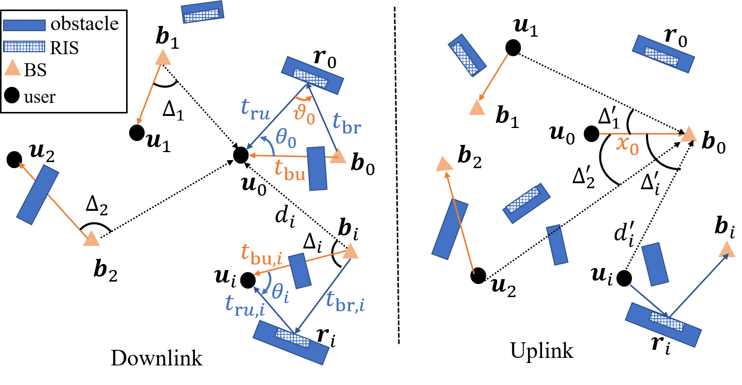
Figure 1: RIS-assisted downlink and uplink communications.

II-B Association Rule

Generally, a user located at $\mathbf{u}_{i}$ is associated with its nearest BS located at $\mathbf{b}_{i}$ with BS-user distance $t_{{\rm bu},i}=||\mathbf{b}_{i}-\mathbf{u}_{i}||$. The BS directly transmits (or receives) signals to (or from) the typical user in the downlink (or uplink) if the direct LoS link exists. However, in the absence of the direct LoS link, NLoS propagation introduces significant attenuation, especially for high-frequency signals, necessitating an alternative association strategy. We consider that the user establishes a connection with its nearest RIS (located at $\mathbf{r}_{i}$) that can provide a cascaded LoS link between the BS and the user, i.e., this RIS satisfies the conditions in Definition 2. Although this rule may not always be optimal, we adopt it to strike a balance between model practicality and analytical simplicity [21, 20]. The distance between $\mathbf{r}_{i}$ and $\mathbf{u}_{i}$ (or $\mathbf{b}_{i}$) is denoted by RIS-user distance $t_{{\rm ru},i}=||\mathbf{r}_{i}-\mathbf{u}_{i}||$ (or BS-RIS distance $t_{{\rm br},i}=||\mathbf{b}_{i}-\mathbf{r}_{i}||$). Moreover, we consider that the link between a BS and its connected RIS is LoS [19, 34]. If neither a direct LoS nor a cascaded LoS link is available, the direct NLoS link is used for downlink/uplink transmission.

From Slivnyak’s theorem [35], the statistics observed at a random point of a PPP are the same as those observed at the origin. Without loss of generality, the following analysis focuses on the typical user located $\mathbf{u}_{0}$ and the tagged BS located at $\mathbf{b}_{0}$ [16]. For notation simplicity, we abbreviate $t_{{\rm bu},0}$, $t_{{\rm ru},0}$, and $t_{{\rm br},0}$ as $t_{\rm bu}$, $t_{\rm ru}$, and $t_{\rm br}$, respectively. As depicted in Fig. 1, by defining the angle from the user-BS link to the user-RIS link as $\theta_{0}$, we can express $t_{\rm br}$ as

$$t_{\rm br}=\sqrt{t_{\rm bu}^{2}+t_{\rm ru}^{2}-2t_{\rm bu}t_{\rm ru}\cos\theta_{0}}.$$ (1)

II-C Antenna Pattern

A BS equipped with a ULA with $N_{\rm b}$ antennas can provide directional beams via analog beamforming. Assume that the beam direction of a BS is aligned at the physical AoD $\phi_{\rm p}^{*}$, which is uniformly distributed, i.e., $\phi_{\rm p}^{*}\sim\mathcal{U}[0,2\pi]$. We define $\phi_{\rm s}^{*}={d}\cos(\phi_{\rm p}^{*})/{\lambda_{f}}$ as the spatial AoD, where $\lambda_{f}$ is the wavelength and $d={\lambda_{f}}/{2}$ is the antenna spacing, i.e., $\phi_{\rm s}^{*}=\frac{1}{2}\cos(\phi_{\rm p}^{*})\in[-\frac{1}{2},\frac{1}{2}]$. The beam gain observed at another physical AoD $\phi_{\rm p}\sim\mathcal{U}[0,2\pi]$ or spatial AoD $\phi_{\rm s}=\frac{1}{2}\cos(\phi_{\rm p})$ is [36]

$$G_{\rm ULA}(\phi_{\rm s}-\phi_{\rm s}^{*})=G_{\rm ULA}(\Delta)=\frac{\sin^{2}(\pi N_{\rm b}\Delta)}{N_{\rm b}\sin^{2}(\pi\Delta)}.$$ (2)

where $\Delta=\phi_{\rm s}-\phi_{\rm s}^{*}\in[-1,1]$ is the spatial AoD deviation off the aligned direction. Note that $G_{\rm ULA}(\cdot)$ is a periodic and even function with $G_{\rm ULA}(\Delta)=G_{\rm ULA}(|\Delta\pm 1|)$.

In the downlink/uplink serving link, a BS aligns the beam direction towards its associated user (or RIS) in the direct (or cascaded) link to provide the maximum antenna gain $G_{\rm b}=G_{\rm ULA}(0)=N_{\rm b}$ [18]. As for the downlink interfering link from a BS at $\mathbf{b}_{i}$ to the typical user at $\mathbf{u}_{0}$ ($i\neq 0$), we define $\Delta_{i}$ as the spatial AoD deviation off the aligned direction $\mathbf{b}_{i}$-$\mathbf{u}_{i}$ observed at $\mathbf{b}_{i}$-$\mathbf{u}_{0}$. The beam gain in the downlink interfering link is $G_{\rm ULA}(\Delta_{i})$. Likewise, the beam gain in the uplink interfering link from user at $\mathbf{u}_{i}$ to the tagged BS at $\mathbf{b}_{0}$ ($i\neq 0$) is $G_{\rm ULA}(\Delta^{\prime}_{i})$, where $\Delta^{\prime}_{i}$ is the spatial AoD deviation off the aligned direction $\mathbf{u}_{0}$-$\mathbf{b}_{0}$ observed at $\mathbf{u}_{i}$-$\mathbf{b}_{0}$, as shown in Fig. 1. For analytical tractability in interference characterization, previous works adopted a flat-top antenna pattern to approximate (2), e.g., [21, 19]. However, the oversimplified flat-top pattern leads to deviations in the network performance analysis [36]. To strike a balance between accuracy and tractability, we adopt the following discrete multi-lobe antenna model in [37] for the subsequent interference analysis, i.e., when $\Delta\in[-\frac{1}{2},\frac{1}{2}]$,

$$G_{\rm B}(\Delta)=\begin{cases}G_{0},&\text{ if }|\Delta|\leq\frac{1}{N_{\rm b}},\\ G_{n},&\text{ if }\frac{n}{N_{\rm b}}<|\Delta|\leq\frac{n+1}{N_{\rm b}},\\ G_{\tilde{N}_{\rm b}+1},&\text{otherwise},\end{cases}$$ (3)

where $G_{n}=\frac{\delta}{2}G_{\rm ULA}(\frac{2n+1}{2N_{\rm b}})$, for $n\in\{1,2,...,\tilde{N}_{\rm b}\}$, $G_{0}=\frac{\delta}{2}G_{\rm ULA}(0)$, and $G_{\tilde{N}_{\rm b}+1}=0$, where $\delta$ is a constant compensation factor for roll-off characteristics in (2), and $\tilde{N}_{\rm b}=\left\lfloor\frac{N_{\rm b}}{2}\right\rfloor-1$. Moreover, for $\Delta\in[-1,-\frac{1}{2})$, $G_{\rm B}(\Delta)=G_{\rm B}(|\Delta+1|)$, and for $\Delta\in(\frac{1}{2},1]$, $G_{\rm B}(\Delta)=G_{\rm B}(|\Delta-1|)$. The accuracy of the discrete antenna model will be verified in Sec. VII.

II-D Channel Model

By modeling the obstacles as line segments, the LoS probability of a link with distance $t$ can be expressed as [38]

$$\mathcal{P}_{\rm L}(t)=\exp\left(-\beta t\right),$$ (4)

where $\beta=\frac{2\lambda_{\rm o}L_{\rm o}}{\pi}$ and $L_{\rm o}=\mathbb{E}[\ell]$ is the average length of line segments (obstacles). The corresponding NLoS probability is $\mathcal{P}_{\rm N}(t)=1-\mathcal{P}_{\rm L}(t)$. The path loss is $\zeta t^{-\alpha_{\rm L}}$ or $\zeta t^{-\alpha_{\rm N}}$, where $\zeta=(\frac{\lambda_{f}}{4\pi})^{2}$ represents the reference path loss and $\alpha_{v}$ ($v\in\{\rm L,N\}$) is the path-loss exponent [27, 31]. We model the small-scale fading as independent Nakagami-m fading with shaping parameter $m_{\rm L}$ ($m_{\rm N}$) for each LoS (NLoS) link, where we assume $m_{\rm L},m_{\rm N}\in\mathbb{N}$ (integers) for analytical simplicity [39]. The CDF and probability density function (PDF) of the small-scale fading coefficient, denoted by $H_{v}$, $v\in\left\{\rm L,\rm N\right\}$, are [40]

$$F_{H_{v}}(h) =\frac{\Gamma_{l}(m_{v},m_{v}h)}{\Gamma(m_{v})},$$ (5a)

$$f_{H_{v}}(h) =\frac{m_{v}^{m_{v}}h^{m_{v}-1}}{\Gamma(m_{v})}e^{-m_{v}h},$$ (5b)

where $\Gamma_{l}\left(m,mg\right)=\int_{0}^{mg}x^{m-1}e^{-x}\mathrm{d}x$ is the lower incomplete Gamma function, $\Gamma\left(m\right)=\int_{0}^{\infty}x^{m-1}e^{-x}\mathrm{d}x$ is the Gamma function, and $\mathbb{E}[H_{v}]=1$. Specifically, in the downlink, we denote the small-scale fading coefficient in the direct LoS/NLoS link between $\mathbf{b}_{0}$ and $\mathbf{u}_{0}$ as $H_{{\rm D}v}$, $v\in\{\rm L,N\}$. $H_{{\rm D}v}$ follows the distribution in (5) with shaping parameter $m_{{\rm D}v}=m_{v}\in\mathbb{N}$. The small-scale fading coefficient in the downlink cascaded LoS link between $\mathbf{b}_{0}$ and $\mathbf{u}_{0}$ is denoted by $H_{{\rm CL}}=H_{\rm bu}H_{\rm ru}$, where $H_{\rm bu}$ and $H_{\rm ru}$ are the small-scale fading coefficients in BS-RIS and RIS-user links. Since the BS-RIS link has strong LoS [19, 34], the shaping parameter of $H_{\rm bu}$ tends to be infinite, i.e., $H_{\rm bu}$ is approximately constant unit. Therefore, we consider that $H_{{\rm CL}}$ follows the same distribution as $H_{\rm ru}$ with shaping parameter $m_{{\rm CL}}=m_{\rm L}\in\mathbb{N}$ in (5) [19]. Similarly, we denote the small-scale fading coefficient in the uplink serving link as $H^{\prime}_{q}$, $q\in\mathcal{S}$, with the same distribution as $H_{q}$.

III Downlink SINR and EMFE

In this section, we present the modeling of downlink SINR and EMFE at the typical user, along with performance metrics to independently characterize the statistics of SINR and EMFE. Moreover, we propose a joint metric to capture their correlation.

III-A Downlink SINR

This subsection quantifies the downlink SINR by analyzing the serving and interference signal power at the typical user.

III-A1 Received Serving Signal Power

When the serving link is direct LoS/NLoS, the tagged BS at $\mathbf{b}_{0}$ aligns the beam with the typical user at $\mathbf{u}_{0}$, providing maximum antenna gain $G_{\rm b}$ [36, 18]. In this case, the received serving signal power at the typical user is

$$P_{{\rm D}v}=p_{\rm b}G_{\rm b}\zeta t_{\rm bu}^{-\alpha_{v}}H_{{\rm D}v}=P^{\rm a}_{{\rm D}v}H_{{\rm D}v},v\in\{\rm L,N\},$$ (6)

where $p_{\rm b}$ is the BS transmit power and $P^{\rm a}_{{\rm D}v}\overset{\bigtriangleup}{=}p_{\rm b}G_{\rm b}\zeta t_{\rm bu}^{-\alpha_{v}}$. When the serving link is cascaded LoS, the BS at $\mathbf{b}_{0}$ aligns the beam direction with its associated RIS at $\mathbf{r}_{0}$ to provide maximum antenna gain $G_{\rm b}$. By appropriately designing the RIS phases, the RIS reflects the incident wave towards the typical user at $\mathbf{u}_{0}$ with maximum RIS gain $G_{\rm r}=N_{\rm r}^{2}$ [18, 21, 19]. The corresponding received serving signal power at the typical user is

$$P_{\rm CL} =p_{\rm b}G_{\rm b}G_{\rm r}\zeta(t_{\rm ru}t_{\rm br})^{-\alpha_{\rm L}}H_{{\rm CL}}=P^{\rm a}_{\rm CL}H_{{\rm CL}},$$ (7)

where $P^{\rm a}_{\rm CL}\overset{\bigtriangleup}{=}p_{\rm b}G_{\rm b}G_{\rm r}\zeta(t_{\rm ru}t_{\rm br})^{-\alpha_{\rm L}}$.

III-A2 Received Interfering Signal Power

The interference experienced by the typical user is dominated by the received interfering signal power from BSs. A BS located at $\mathbf{b}_{i}$ may interfere with the typical user at $\mathbf{u}_{0}$ via a LoS (or NLoS) link with probability $\mathcal{P}_{\rm L}(d_{i})$ (or $\mathcal{P}_{\rm N}(d_{i})$), where $d_{i}=||\mathbf{b}_{i}-\mathbf{u}_{0}||$. Therefore, we have $\Psi_{\rm b}=\Psi_{\rm b,L}\cup\Psi_{\rm b,N}$, where the link between the BS at $\mathbf{b}_{i}\in\Psi_{\rm b,L}$ (or $\Psi_{\rm b,N}$) and the typical user is LoS (or NLoS). The density of $\Psi_{{\rm b},v}$ is $\lambda_{\rm b}\mathcal{P}_{v}(d_{i})$, where $v\in\{\rm L,N\}$. The interference from BSs in $\Psi_{{\rm b},v}$, ${v\in\{\rm L,N\}}$, is

$$I_{{\rm b},v}=\sum_{i,\mathbf{b}_{i}\in\Psi_{{\rm b},v}\setminus\{\mathbf{b}_{0}\}}{p_{\rm b}G_{\rm B}(\Delta_{i})\zeta d_{i}^{-\alpha_{v}}H_{v,i}},$$ (8)

where $G_{\rm B}(\Delta_{i})$ is antenna gain of the BS at $\mathbf{b}_{i}$, $d_{i}=||\mathbf{b}_{i}-\mathbf{u}_{0}||$, $H_{v,i}$ is the small-scale fading coefficient of the interfering link, and $H_{v,i}$ follows the distribution in (5). Therefore, the aggregate interference from BSs is $I_{\rm B}=I_{\rm b,L}+I_{\rm b,N}$.

III-A3 Downlink SINR and Coverage Probability

The probability that the downlink SINR ($\Upsilon$) is above a predefined threshold ($\gamma$) is defined as the downlink coverage probability, denoted by $\bar{F}_{\Upsilon}(\gamma)$. Namely, $\bar{F}_{\Upsilon}(\gamma)$ is the CCDF of $\Upsilon$, i.e.,

$$\bar{F}_{\Upsilon}(\gamma) =\mathbb{P}\left({\Upsilon}>\gamma\right).$$ (9)

Considering that the serving link may be direct LoS, cascaded LoS, or direct NLoS, the corresponding downlink SINR, denoted by $\Upsilon_{q}$, is

$${\Upsilon}_{q}=\frac{P_{q}}{\sigma^{2}+I_{\rm B}},q\in\mathcal{S},$$ (10)

where $\sigma^{2}$ is the noise power in the downlink. Then, based on the total probability law, we can express (9) as

$$\bar{F}_{\Upsilon}(\gamma) =\sum_{q\in\mathcal{S}}\mathbb{P}\left({\Upsilon_{q}}>\gamma\right)\mathcal{A}_{q},$$ (11)

where $\mathcal{A}_{q}$ is the association probability, e.g., $\mathcal{A}_{\rm DL}$ is the probability that the typical user is associated with the tagged BS via the direct LoS link, which will be analyzed in Sec. IV-A.

III-B Downlink EMFE

In the RIS-assisted downlink communication, EMFE is introduced by BS transmission and RIS reflection, which can be quantified by the received power density at the typical user [23].

III-B1 Received Power Density

Based on the received serving signal power $P_{q}$ given in (6) and (7), the received serving signal power density at the typical user is

$$\mathcal{W}_{1,q} =\frac{P_{q}}{\mathcal{E}}=\frac{P^{\rm a}_{q}H_{q}}{\mathcal{E}},$$ (12)

where $q\in\mathcal{S}$ is the serving link type, $\mathcal{E}=\frac{\lambda_{f}^{2}G_{\rm u}}{4\pi}$ is the antenna effective area of the typical user, and $G_{\rm u}\!=\!1$ for the single-antenna user. Similarly, from (8), the received interfering signal power density at the typical user is

$$\mathcal{W}_{2} =\frac{I_{\rm B}}{\mathcal{E}}=\frac{I_{\rm b,L}+I_{\rm b,N}}{\mathcal{E}}=\mathcal{W}_{\rm b,L}+\mathcal{W}_{\rm b,N},$$ (13)

where $\mathcal{W}_{{\rm b},v}\overset{\bigtriangleup}{=}\frac{I_{{\rm b},v}}{\mathcal{E}}$. Therefore, considering the type of the serving link $q\in\mathcal{S}$, the aggregate downlink EMFE, denoted by $\mathcal{W}_{q}~\left[\rm W/m^{2}\right]$, is

$$\mathcal{W}_{q} =\mathcal{W}_{1,q}+\mathcal{W}_{2}=\frac{P_{q}+I_{\rm B}}{\mathcal{E}}.$$ (14)

III-B2 Downlink EMFE Constraint and Compliance Probability

The probability that the downlink EMFE ($\mathcal{W}$) is below a constraint level ($\omega$), i.e., the CDF of EMFE, is defined as the downlink compliance probability, denoted by $F_{\mathcal{W}}(\omega)$. The lower the EMFE, the higher the compliance probability. Similar to (11), the downlink compliance probability can be written as

$$F_{\mathcal{W}}(\omega) =\mathbb{P}(\mathcal{W}\leq\omega)=\sum_{q\in\mathcal{S}}\mathbb{P}({\mathcal{W}_{q}}\leq\omega)\mathcal{A}_{q}.$$ (15)

Regulatory authorities have imposed a constraint on EMFE, requiring it to remain below the maximum allowed value $\mathcal{W}_{\max}$ with high probability $\rho$ [41], i.e., $F_{\mathcal{W}}(\mathcal{W}_{\max})\geq\rho$. We can express the EMFE constraint as

$$F^{-1}_{\mathcal{W}}(\rho)\leq\mathcal{W}_{\max},$$ (16)

where $F^{-1}_{\mathcal{W}}(\rho)$ is the inverse function of $F_{\mathcal{W}}(\omega)$ in (15). From [3], $\mathcal{W}_{\max}=10~\rm W/m^{2}$ and $\rho=0.95$. In particular, we define $F^{-1}_{\mathcal{W}}(0.95)$ as 95-th percentile of EMFE, which means the probability that the EMFE exceeds $F^{-1}_{\mathcal{W}}(0.95)$ is below 5%.

III-C Joint Metric of Downlink SINR and EMFE

From the above discussion, we observe that the statistical characteristics of downlink SINR ($\Upsilon$) and EMFE ($\mathcal{W}$) are correlated via the distance, the small-scale fading, and the type of the serving link. Therefore, instead of independently analyzing the downlink SINR or EMFE distribution by the downlink coverage or compliance probability, we define a joint metric as follows.

Definition 4 (Joint Coverage and Compliance Probability).

The probability that both (i) SINR is above a predefined threshold, and (ii) EMFE is below a constraint level, is defined as the joint coverage and compliance probability, abbreviated as joint probability. A high joint probability is achieved when SINR is high and EMFE is low.

The downlink joint probability, denoted by $J_{\Upsilon,\mathcal{W}}(\gamma,\omega)$, is

$$\begin{split}J_{\Upsilon,\mathcal{W}}(\gamma,\omega)&=\mathbb{P}({\Upsilon}>\gamma,\mathcal{W}\leq\omega)\\ &=\sum_{q\in\mathcal{S}}\mathbb{P}(\Upsilon_{q}>\gamma,\mathcal{W}_{q}\leq\omega)\mathcal{A}_{q}.\end{split}$$ (17)

From Definition 4, the joint probability allows for a quantified assessment of both SINR and EMFE. This is particularly useful in cases where deployment strategies are designed to improve SINR while potentially exacerbating EMFE. Using the joint probability, alternative strategies can be explored to balance SINR and EMFE.

IV Downlink Performance Analysis

This section derives the expressions for the downlink performance metrics. We first provide the association probabilities and the distance distributions of different serving links. Then, we derive the downlink coverage and compliance probabilities independently, i.e., the marginal distributions of $\Upsilon$ and $\mathcal{W}$. We also derive the first moment of $\mathcal{W}$. Based on the EMFE distribution, we investigate the CD. Finally, we derive the joint distribution of $\Upsilon$ and $\mathcal{W}$.

IV-A Association Probability

IV-A1 Association with a Direct LoS Link

From Sec. II-B, the probability that the typical user located at $\mathbf{u}_{0}$ is associated with the BS located at $\mathbf{b}_{0}$ via the direct LoS link is the LoS probability of the direct link, i.e., $\mathcal{A}_{\rm DL}=\mathcal{P}_{\rm L}(t_{\rm bu})$.

IV-A2 Association with a Cascaded LoS Link

Recall that there are two independent conditions of the cascade LoS link in Definition 2. For a RIS located at $\mathbf{r}$, a cascaded LoS link between the typical user at $\mathbf{u}_{0}$ and the tagged BS at $\mathbf{b}_{0}$ exists if the RIS satisfies (i) LoS condition of the BS-RIS and RIS-user links and (ii) reflection condition. Considering that the BS-RIS link is strong LoS [19, 34], the probability that the RIS satisfies condition (i) is the LoS probability of the user-RIS link, i.e., $\mathcal{P}_{\rm L}(t)$, where $t=||\mathbf{r}-\mathbf{u}_{0}||$. The probability of the RIS satisfying condition (ii) is [17, Appendix A]

$$\mathcal{P}_{\rm R}(t_{\rm bu},t,\theta)\!=\!\!\frac{1}{2}\!-\!\frac{1}{2\pi}\arccos\!\left(\!\!\frac{t-t_{\rm bu}\cos\theta}{\sqrt{t_{\rm bu}^{2}\!+\!t^{2}\!-\!2t_{\rm bu}t\cos\theta}}\!\!\right)\!,$$ (18)

where $\theta\sim\mathcal{U}(-\pi,\pi)$ is the angle from the user-BS link to the user-RIS link. Then, the probability that the RIS at $\mathbf{r}$ can create a cascaded LoS link between $\mathbf{u}_{0}$ and $\mathbf{b}_{0}$ is

$$a(t_{\rm bu},t,\theta)=\mathcal{P}_{\rm L}(t_{\rm ru})\mathcal{P}_{\rm R}(t_{\rm bu},t,\theta).$$ (19)

To establish a cascaded LoS link between $\mathbf{u}_{0}$ and $\mathbf{b}_{0}$, it is necessary that at least one RIS in $\Psi_{\rm r}$ satisfies the above two conditions. Therefore, the probability of the existence of a cascaded LoS link between $\mathbf{u}_{0}$ and $\mathbf{b}_{0}$ is [17, Lemma 2]

$$\mathcal{P}_{\rm CL}(t_{\rm bu})=1-\exp\left(-\lambda_{\rm r}\int_{0}^{\infty}\bar{a}(t_{\rm bu},t)t\,{\rm d}t\right),$$ (20)

where $\bar{a}(t_{\rm bu},t)=\int_{-\pi}^{\pi}a(t_{\rm bu},t,\theta)\mathrm{d}\theta$. As discussed in Sec. II-B, the serving link is cascaded LoS if the direct LoS link is unavailable and if the cascaded LoS link exists. Hence, we have $\mathcal{A}_{\rm CL}=\mathcal{P}_{\rm N}(t_{\rm bu})\mathcal{P}_{\rm CL}(t_{\rm bu})$.

IV-A3 Association with a Direct NLoS Link

The probability of associating with a direct NLoS link is $\mathcal{A}_{\rm DN}=1-\mathcal{A}_{\rm DL}-\mathcal{A}_{\rm CL}=\mathcal{P}_{\rm N}(t_{\rm bu})(1-\mathcal{P}_{\rm CL}(t_{\rm bu}))$.

IV-B Beam Gain Distribution

With the discrete antenna model $G_{\rm B}(\Delta)$ in (3), we discretize the antenna gain as a constant $G_{n}$, $n\in\{1,2,...,\tilde{N}_{\rm b}\}$, at different intervals of $\Delta$. For the subsequent interference analysis, we provide the probability of the antenna gain being $G_{n}$ based on the distribution of $\Delta$ in the following.

We denote the PDF of $\Delta$ as $f_{\Delta}(\cdot)$. As defined in Sec. II-C, $\Delta=\phi_{\rm s}-\phi_{\rm s}^{*}=\frac{1}{2}\cos(\phi_{\rm p})-\frac{1}{2}\cos(\phi_{\rm p}^{*})$. Based on the uniform distribution of the physical AoDs $\phi_{\rm p}$ and $\phi_{\rm p}^{*}$ in $[0,2\pi]$, the probability density function (PDF) of $\Delta$ is

$$f_{\Delta}(y)=\begin{cases}\int_{-\frac{1}{2}}^{\frac{1}{2}}f_{\Phi}(x)f_{\Phi}(y+x)\mathrm{d}x,&\text{for }y\in[-1,1],\\ 0,&\text{otherwise},\end{cases}$$ (21)

where $f_{\Phi}(\cdot)$ is the PDF of $\phi_{\rm s}$ and $\phi_{\rm s}^{*}$. Based on the uniform distribution of $\phi_{\rm p}$, we have $f_{\Phi}(x)=\frac{2}{\pi\sqrt{1-4x^{2}}}$ for $x\in[-\frac{1}{2},\frac{1}{2}]$.

Lemma 1.

Under the discrete antenna model $G_{\rm B}(\Delta)$ in (3), the probability that the beam gain is $G_{n}$ is given by

$$p_{n} =2\int_{\frac{n}{N_{\rm b}}}^{\frac{n+1}{N_{\rm b}}}f_{\Delta}(y)\mathrm{d}y+2\int_{1-\frac{n+1}{N_{\rm b}}}^{1-\frac{n}{N_{\rm b}}}f_{\Delta}(y)\mathrm{d}y,$$ (22)

where $n\in\{0,1,...,\tilde{N}_{\rm b}\}$ and $\tilde{N}_{\rm b}=\left\lfloor\frac{N_{\rm b}}{2}\right\rfloor-1$. The probability that the beam gain is $G_{\tilde{N}_{b}+1}=0$ is $p_{\tilde{N}_{b}+1}=1-\sum_{n=0}^{\tilde{N}_{b}}p_{n}$.

Proof:

From (3), when $\Delta\in(\frac{n}{N_{\rm b}},\frac{n+1}{N_{\rm b}}]\cup[1-\frac{n+1}{N_{\rm b}},1-\frac{n}{N_{\rm b}})\cup(\frac{n}{N_{\rm b}}-1,\frac{n+1}{N_{\rm b}}-1]\cup[-\frac{n+1}{N_{\rm b}},-\frac{n}{N_{\rm b}})$, we have $G_{\rm B}(\Delta)=G_{n}$. Based on $f_{\Delta}(\cdot)$ in (21), we obtain (22). ∎

Note that $p_{n}$ depends on the antenna number $N_{\rm b}$. Given $N_{\rm b}$, $p_{n}$ can be numerically calculated offline, which will greatly simplify the subsequent interference analysis.

IV-C Serving Link Distance Distribution

From Sec. II-B, the typical user is served by its nearest BS. Based on the null probability of a PPP, the PDF of the BS-user distance $t_{\rm bu}$ in the direct link is [16]

$$f_{T_{\rm bu}}(t_{\rm bu}) =2\pi\lambda_{\rm b}t_{\rm bu}\exp(-\pi\lambda_{\rm b}t_{\rm bu}^{2}).$$ (23)

We provide the distribution of RIS-user distance $t_{\rm ru}$ in the following lemma.

Lemma 2.

Conditioned on the BS-user distance $t_{\rm bu}$, the PDF of the RIS-user distance $t_{\rm ru}$ in the cascaded link is

$$f_{T_{\rm ru}|t_{\rm bu}}(t_{\rm ru})=\frac{\lambda_{\rm r}t_{\rm ru}\bar{a}(t_{\rm bu},t_{\rm ru})\exp(-\lambda_{\rm r}\int_{0}^{t_{\rm ru}}\bar{a}(t_{\rm bu},t)t\mathrm{d}t)}{\mathcal{P}_{\rm CL}(t_{\rm bu})}.$$ (24)

Proof:

Based on the reflection probability in (19) and the void probability of a PPP, we can finish the derivation [1]. ∎

Given $t_{\rm ru}$ and $t_{\rm bu}$, the distribution of BS-RIS distance $t_{\rm br}$ is dependent on $\theta_{0}\sim\mathcal{U}(-\pi,\pi)$, as shown in (1).

IV-D Downlink SINR Analysis

Let $\mathcal{T}_{q}$ be the set of random variables relevant to the distances of different types of the serving link, i.e., $\mathcal{T}_{\rm DL}=\mathcal{T}_{\rm DN}=\{t_{\rm bu}\}$, $\mathcal{T}_{\rm CL}=\{t_{\rm bu},t_{\rm ru},t_{\rm br}\}$. Then, we can define the conditional coverage probability as the CCDF of ${\Upsilon}_{q}$ conditioned on $\mathcal{T}_{q}$, denoted by $\bar{F}_{{\Upsilon}_{q}|\mathcal{T}_{q}}(\gamma)$. For Nakagami-m parameter $m_{q}\in\mathbb{N}$, $q\in\mathcal{S}$, $\bar{F}_{{\Upsilon}_{q}|\mathcal{T}_{q}}(\gamma)$ is given by [39, 20]

$$\bar{F}_{{\Upsilon}_{q}|\mathcal{T}_{q}}(\gamma)=\mathbb{P}({\Upsilon}_{q}>\gamma|\mathcal{T}_{q})$$

$$\overset{(a)}{=}\sum_{k=0}^{m_{q}-1}\frac{s_{q}^{k}}{k!}\left(-1\right)^{k+1}\frac{\mathrm{d}^{k}}{\mathrm{d}^{k}s_{q}}\mathcal{L}_{I_{\rm B}|t_{\rm bu}}(s_{q})$$

$$\overset{(b)}{\approx}\sum_{k=1}^{m_{q}}\!\binom{m_{q}}{k}(-1)^{k+1}\!\exp(-k\beta_{q}s_{q}\sigma^{2})\mathcal{L}_{I_{\rm B}|t_{\rm bu}}(k\beta_{q}s_{q}),$$ (25)

where $s_{q}=\frac{m_{q}\gamma}{P^{\rm a}_{q}}$, $P^{\rm a}_{q}$ is given in (6) and (7), $\beta_{q}=\left(m_{q}!\right)^{\frac{-1}{m_{q}}}$, $\mathcal{L}_{I_{\rm B}|t_{\rm bu}}(s)=\mathbb{E}\left[\exp\left(-sI_{\rm B}\right)\right]$ is derived in the following lemma, the calculation in (a) would be quite complex due to the high order of derivations of the Laplace transform, and (b) provides an approximate expression to simplify the computation by using the upper bound of the CDF of the Gamma distribution [39, Appendix F].

Lemma 3.

The Laplace transform of $I_{\rm B}$ conditioned on $t_{\rm bu}$ is

$$\mathcal{L}_{I_{{\rm B}}|t_{\rm bu}}(s) =\!\!\!\prod_{v\in\{\rm L,N\}}\!\!\exp\bigg{(}\!\!-2\pi\lambda_{\rm b}\times$$

$$\int_{t_{\rm bu}}^{\infty}\!\!\![1-\kappa_{v}({sp_{\rm b}\zeta}{d_{i}^{-\alpha_{v}}})]d_{i}\mathcal{P}_{v}(d_{i})\mathrm{d}d_{i}\bigg{)},$$ (26)

where $\kappa_{v}(x)=\sum_{n=0}^{\tilde{N}_{\rm b}+1}p_{n}\left(1+\frac{xG_{n}}{m_{v}}\right)^{-m_{v}}$, $G_{n}$ is given in (3), $p_{n}$ is given in (22), and $\mathcal{P}_{v}(\cdot)$ is the LoS (or NLoS) probability for $v={\rm L}$ (or $v={\rm N}$).

Proof:

See Appendix A. ∎

With the conditional coverage probability $\bar{F}_{{\Upsilon}_{q}|\mathcal{T}_{q}}(\gamma)$, we derive the downlink coverage probability as follows.

Theorem 1 (Downlink Coverage Probability).

The CCDF of the downlink SINR ($\Upsilon$) in (11) is

$$\begin{split}&\bar{F}_{\Upsilon}(\gamma)=\mathbb{E}_{t_{\rm bu},t_{\rm ru},t_{\rm br}}\bigg{[}\sum_{q\in\mathcal{S}}\mathcal{A}_{q}\bar{F}_{{\Upsilon}_{q}|\mathcal{T}_{q}}(\gamma)\bigg{]}\\ &\overset{(a)}{=}\mathbb{E}_{t_{\rm bu},t_{\rm ru},\theta_{0}}\bigg{[}\sum_{q\in\mathcal{S}}\mathcal{A}_{q}\bar{F}_{{\Upsilon}_{q}|\mathcal{T}_{q}}(\gamma)\bigg{]}\\ &=\int_{0}^{\infty}\bigg{[}\mathcal{A}_{\rm DL}\bar{F}_{{\Upsilon}_{\rm DL}|t_{\rm bu}}(\gamma)\\ &+\int_{0}^{\infty}\int_{-\pi}^{\pi}\mathcal{A}_{\rm CL}\bar{F}_{{\Upsilon}_{\rm CL}|t_{\rm bu},t_{\rm ru},\theta_{0}}(\gamma){\frac{1}{2\pi}f_{T_{\rm ru}|t_{\rm bu}}(t_{\rm ru})\mathrm{d}\theta_{0}\mathrm{d}t_{\rm ru}}\\ &+\mathcal{A}_{\rm DN}\bar{F}_{{\Upsilon}_{\rm DN}|t_{\rm bu}}(\gamma)\bigg{]}f_{T_{\rm bu}}(t_{\rm bu})\mathrm{d}t_{\rm bu},\end{split}$$ (27)

where (a) is from (1), and $\bar{F}_{{\Upsilon}_{\rm CL}|t_{\rm bu},t_{\rm ru},\theta_{0}}$ is obtained by substituting (1) into (IV-D).

To simplify the expressions in the subsequent analysis, we do not expand the expectation operation over $t_{\rm bu}$, $t_{\rm ru}$, and $t_{\rm br}$, i.e., $\mathbb{E}_{t_{\rm bu},t_{\rm ru},t_{\rm br}}[\cdot]$ can be conducted in the same way as (27).

IV-E Downlink EMFE Analysis

The CDF of $\mathcal{W}_{q}$ conditioned on $\mathcal{T}_{q}$, i.e., conditional compliance probability, denoted by $F_{\mathcal{W}_{q}|\mathcal{T}_{q}}(\omega)$, $q\in\mathcal{S}$, is given by [23, Appendix C]

$$F_{\mathcal{W}_{q}|\mathcal{T}_{q}}(\omega)=\mathbb{P}(\mathcal{W}_{q}\leq\omega|\mathcal{T}_{q})$$

$$\overset{(a)}{=}\frac{1}{2}-\int_{0}^{\infty}\frac{1}{\pi x}{\rm Im}\big{[}e^{-{j}x\omega}\mathcal{L}_{\mathcal{W}_{q}|\mathcal{T}_{q}}(-{j}x)\big{]}{\rm d}x.$$ (28)

where (a) is from Gil-Pelaez’s inversion theorem [42], ${\rm Im}(s)$ is the imaginary part of $s$, $j$ is the imaginary unit with $j^{2}=-1$, and $\mathcal{L}_{\mathcal{W}_{q}|\mathcal{T}_{q}}(s)=\mathbb{E}\left[\exp(-s\mathcal{W}_{q})\right]$ is derived below.

Lemma 4.

The Laplace transform of $\mathcal{W}_{q}$ conditioned on $\mathcal{T}_{q}$ is

$$\mathcal{L}_{\mathcal{W}_{q}|\mathcal{T}_{q}}(s) =\left(1+\frac{sP^{\rm a}_{q}}{m_{q}\mathcal{E}}\right)^{-m_{q}}\ \!\!\!\!\!\!\mathcal{L}_{\mathcal{W}_{2}|t_{\rm bu}}(s),$$ (29)

where $\mathcal{L}_{\mathcal{W}_{2}|t_{\rm bu}}(s)=\mathcal{L}_{\mathcal{W}_{\rm b,L}|t_{\rm bu}}(s)\mathcal{L}_{\mathcal{W}_{\rm b,N}|t_{\rm bu}}(s)$,

$$\begin{split}&\mathcal{L}_{\mathcal{W}_{{\rm b},v}|t_{\rm bu}}(s)\!=\!\exp\bigg{(}\!\!\!-\!2\pi\lambda_{\rm b}\!\!\int_{t_{\rm bu}}^{\infty}\!\!\!\![1-\kappa_{v}(\frac{sp_{\rm b}}{4\pi d_{i}^{\alpha_{v}}})]d_{i}\mathcal{P}_{v}(d_{i})\mathrm{d}d_{i}\!\!\bigg{)},\end{split}$$

$v\in\{L,N\}$, and $\kappa_{v}(\cdot)$ is given in Lemma 3.

Proof:

From (14), we have

$$\mathcal{L}_{\mathcal{W}_{q}|\mathcal{T}_{q}}(s) =\mathbb{E}\left[\exp(-s\mathcal{W}_{q})\right]=\mathbb{E}\left[\exp\left(-s(\mathcal{W}_{1,q}+\mathcal{W}_{2})\right)\right]$$

$$=\mathbb{E}\left[\exp\left(-s\mathcal{W}_{1,q}\right)\right]\times\mathbb{E}\left[\exp\left(-s\mathcal{W}_{2}\right)\right]$$

$$\overset{(a)}{=}\left(1+\frac{sP^{\rm a}_{q}}{m_{q}\mathcal{E}}\right)^{-m_{q}}\ \!\!\!\!\!\!\mathcal{L}_{\mathcal{W}_{2}|t_{\rm bu}}(s),$$ (30)

where (a) is from (5) and $\mathcal{L}_{\mathcal{W}_{2}|t_{\rm bu}}(s)\triangleq\mathbb{E}\left[\exp\left(-s\mathcal{W}_{2}\right)\right]$. We can derive $\mathcal{L}_{\mathcal{W}_{2}|t_{\rm bu}}(s)$ using the same methods in Appendix A, which is omited here. ∎

By averaging (IV-E) over distances $t_{\rm bu}$, $t_{\rm ru}$, or $t_{\rm br}$ with the distributions derived in Sec. IV-C, we obtain the CDF of the EMFE $\mathcal{W}$ in (15) and $\mathbb{E}[\mathcal{W}]$ in the following theorem.

Theorem 2 (Downlink EMFE).

The CDF of overall EMFE $\mathcal{W}$ in (15) is

$$F_{\mathcal{W}}(\omega)=\mathbb{E}_{t_{\rm bu},t_{\rm ru},t_{\rm br}}\bigg{[}\sum_{q\in\mathcal{S}}\mathcal{A}_{q}F_{\mathcal{W}_{q}|\mathcal{T}_{q}}(\omega)\bigg{]},$$ (31)

where $\mathcal{A}_{q}$ is given in Sec. IV-A, $F_{\mathcal{W}_{q}|\mathcal{T}_{q}}(\omega)$ is given in (IV-E), and $\mathbb{E}_{t_{\rm bu},t_{\rm ru},t_{\rm br}}[\cdot]$ can be conducted in the same way as (27). Moreover, the first moment of $\mathcal{W}$ is $\mathbb{E}[\mathcal{W}]=\mathbb{E}[\mathcal{W}_{1}]+\mathbb{E}[\mathcal{W}_{2}]$, where $\mathbb{E}[\mathcal{W}_{1}]$ and $\mathbb{E}[\mathcal{W}_{2}]$ are related to the received serving and interfering signal power density, respectively, i.e.,

$$\mathbb{E}[\mathcal{W}_{1}] =\mathbb{E}_{t_{\rm bu},t_{\rm ru},t_{\rm br}}\bigg{[}\sum_{q\in\mathcal{S}}\frac{P^{\rm a}_{q}}{\mathcal{E}}\mathcal{A}_{q}\bigg{]},$$ (32a)

$$\mathbb{E}[\mathcal{W}_{2}] =\frac{\lambda_{\rm b}p_{\rm b}\bar{g}_{\rm B}}{2}\bigg{(}\mathbb{E}_{t_{\rm bu}}\bigg{[}t_{\rm bu}^{2-\alpha_{\rm L}}{\rm E}_{\alpha_{\rm L}-1}(\beta t_{\rm bu})\bigg{]}+$$

$$\quad\mathbb{E}_{t_{\rm bu}}\bigg{[}\frac{t_{\rm bu}^{2-\alpha_{\rm N}}}{\alpha_{\rm N}-2}-t_{\rm bu}^{2-\alpha_{\rm N}}{\rm E}_{\alpha_{\rm N}-1}(\beta t_{\rm bu})\bigg{]}\bigg{)},$$ (32b)

where $P^{\rm a}_{q}$ is given in (6) and (7), $\bar{g}_{\rm B}=\mathbb{E}_{\Delta}[G_{\rm B}(\Delta)]=\sum_{n=0}^{\tilde{N}_{\rm b}}G_{n}p_{n}$ is from Lemma 1, $\beta=\frac{2\lambda_{\rm o}L_{\rm o}}{\pi}$, ${\rm E}_{n}(x)=\int_{1}^{\infty}\frac{\exp\left(-xt\right)}{t^{n}}\mathrm{d}t$ can be evaluated by a built-in function ${\rm expint}(n,x)$ in Matlab.

Proof:

See Appendix B. ∎

The first-moment analysis of downlink EMFE reveals that a lower BS density ($\lambda_{\rm b}$) decreases the average EMFE from interfering links, i.e., $\mathbb{E}[\mathcal{W}_{2}]$, due to the reducing number of radiating sources. Moreover, by noting that $\mathbb{E}[\mathcal{W}_{2}]$ is primarily influenced by its first term in (32) (i.e., received interfering power density via LoS links) and ${\rm E}_{n}(x)$ is a decreasing function, we find that a higher obstacle density ($\lambda_{\rm o}$), i.e., larger $\beta$, results in a lower value of $\mathbb{E}[\mathcal{W}_{2}]$. These insights underscore the less significant impact of received interfering power density in EMFE, especially in environments with dense obstacles or sparse BSs.

IV-F Compliance Distance

The CD around a BS, denoted by $\tau_{\rm bu}$, represents the minimum allowable separation between a BS and a user, ensuring compliance with the EMFE constraint in (16). Specifically, if the serving BS is located at a distance of $\tau_{\rm bu}$ to the typical user, the corresponding EMFE must not exceed the maximum allowable limit $\mathcal{W}_{\max}$ with high probability $\rho$ [23]. For safety, the worst-case EMFE from BSs, i.e., $\mathcal{W}_{\rm DL}$, should be considered in designing $\tau_{\rm bu}$. Mathematically,

$$\tau_{\rm bu}\triangleq\inf_{t_{\rm bu}\in\mathbb{R}}\left\{t_{\rm bu}:F_{\mathcal{W}_{\rm DL}|t_{\rm bu}}(\mathcal{W}_{\max})\geq\rho\right\}.$$ (33)

From (16), $\tau_{\rm bu}$ satisfies $F^{-1}_{\mathcal{W}_{\rm DL}|\tau_{\rm bu}}(\rho)=\mathcal{W}_{\max}$. Clearly, access to the area centered around a BS with a radius of $\tau_{\rm bu}$ is strictly prohibited as individuals within that area have a high possibility of experiencing EMFE larger than $\mathcal{W}_{\max}$. Conversely, areas beyond the radius of $\tau_{\rm bu}$ are permissible as the EMFE remains within the acceptable limit $\mathcal{W}_{\max}$ with a high probability.

It is worth considering whether a similar CD should be set to account for the EMFE from RIS reflection. As shown in Sec. III-B, if the typical user at $\mathbf{u}_{0}$ establishes a cascaded link with the BS at $\mathbf{b}_{0}$ aided by the RIS at $\mathbf{r}_{0}$, the RIS can potentially lead to significant EMFE. In this case, the aggregate downlink EMFE is $\mathcal{W}_{\rm CL}$ in (14). Therefore, we define the CD for the RIS, denoted by $\tau_{\rm ru}$, as

$$\tau_{\rm ru}\triangleq\inf_{t_{\rm ru}\in\mathbb{R}}\left\{t_{\rm ru}:F_{\mathcal{W}_{\rm CL}|t_{\rm ru}}(\mathcal{W}_{\max})\geq\rho\right\},$$ (34)

where $F_{\mathcal{W}_{\rm CL}|t_{\rm ru}}(\omega)=\mathbb{E}_{t_{\rm bu},t_{\rm br}}[F_{\mathcal{W}_{\rm CL}|t_{\rm bu},t_{\rm ru},t_{\rm br}}(\omega)]$. Furthermore, due to the passive nature of the RIS and its limited signal processing capability, the RIS is usually controlled by the BS [5]. As a result, the BS-RIS distance $t_{\rm br}$ is known in practical scenarios. Moreover, when $t_{\rm ru}$ and $t_{\rm br}$ are given,

$$t_{\rm bu}=\sqrt{t_{\rm ru}^{2}+t_{\rm br}^{2}-2t_{\rm ru}t_{\rm br}\cos\vartheta_{0}},$$ (35)

where $\vartheta_{0}$ is the included angle between RIS-user and RIS-BS links, as shown in Fig. 1. Therefore, we propose a metric for designing the conditional CD of the RIS as follows.

$$\hat{\tau}_{\rm ru}(t_{\rm br})\triangleq\!\!\inf_{t_{\rm ru}\in\mathbb{R}}\!\!\left\{t_{\rm ru}\!:\!F_{\mathcal{W}_{\rm CL}|t_{\rm ru},t_{\rm br}}(\mathcal{W}_{\max})\geq\rho\right\},$$ (36)

where $F_{\mathcal{W}_{\rm CL}|t_{\rm ru},t_{\rm br}}(\omega)=\mathbb{E}_{\vartheta_{0}}[F_{\mathcal{W}_{\rm CL}|\vartheta_{0},t_{\rm ru},t_{\rm br}}(\omega)]$, where $F_{\mathcal{W}_{\rm CL}|\vartheta_{0},t_{\rm ru},t_{\rm br}}(\omega)$ is obtained by substituting (35) into (IV-D). Specifically, $\hat{\tau}_{\rm ru}$ is the minimum allowable separation between the RIS and the user conditioned on $t_{\rm br}$. For clarity, we refer to $\tau_{\rm ru}$ and $\hat{\tau}_{\rm ru}$ as average and conditional CDs of the RIS, respectively. From (16), $\tau_{\rm ru}$ and $\hat{\tau}_{\rm ru}$ satisfy $F^{-1}_{\mathcal{W}_{\rm CL}|\tau_{\rm ru}}(\rho)=\mathcal{W}_{\max}$ and $F^{-1}_{\mathcal{W}_{\rm CL}|\hat{\tau}_{\rm ru},t_{\rm br}}(\rho)=\mathcal{W}_{\max}$.

From the above discussion, $\tau_{\rm bu}$, $\hat{\tau}_{\rm ru}$, and $\tau_{\rm bu}$ can be identified as the optimal solutions of the optimization problems formulated in (33), (34), and (36), respectively. These optimization problems can be solved by efficient one-dimension search algorithms such as bi-sectional [43] or golden section methods [44]. To facilitate more efficient identification on CDs, we further provide approximate closed-form expressions for $\tau_{\rm bu}$, $\hat{\tau}_{\rm ru}$ and $\tau_{\rm bu}$. It is important to note that the exposure is primarily dominated by the received serving power density, especially when the serving link distances are short. Moreover, the CDs are typically quite short [23]. Based on these observations, we ignore the exposure caused by the interfering signals, i.e., $\mathcal{W}_{2}$, which allows us to derive approximate CDs as follows.

Proposition 1 (Compliance Distance).

Considering that the EMFE caused by the serving signals is dominant when the serving link distances are quite short, the BS CD, conditional RIS CD, and average RIS CD can be approximated as

$$\tau_{\rm bu}\approx\bigg{(}\frac{p_{\rm b}G_{\rm b}}{4\pi\mathcal{W}_{\max}}F_{H_{\rm L}}^{-1}(\rho)\bigg{)}^{\frac{1}{\alpha_{\rm L}}},$$ (37)

$$\hat{\tau}_{\rm ru}(t_{\rm br})\approx\bigg{(}\frac{p_{\rm b}G_{\rm b}G_{\rm r}t_{\rm br}^{-\alpha_{\rm L}}}{4\pi\mathcal{W}_{\max}}F_{H_{\rm L}}^{-1}(\rho)\bigg{)}^{\frac{1}{\alpha_{\rm L}}},$$ (38)

$$\tau_{\rm ru}\approx\bigg{(}\frac{p_{\rm b}G_{\rm b}G_{\rm r}}{4\pi\mathcal{W}_{\max}}F_{\alpha_{\rm L}}^{-1}(\rho)\bigg{)}^{-\alpha_{\rm L}},$$ (39)

where $F_{H_{\rm L}}^{-1}(\rho)$ is the inverse function of $F_{H_{\rm L}}(h)$ given in (5a), $F_{\alpha_{\rm L}}^{-1}(\rho)$ is the inverse function of $F_{\alpha_{\rm L}}(h)$, and

$$F_{\alpha_{\rm L}}(h)\!=\!\frac{\alpha_{\rm L}(m_{\rm L}h)^{m_{\rm L}}}{\Gamma(m_{\rm L})}\!\!\int_{0}^{\infty}\!\!t^{m_{\rm L}\alpha_{\rm L}-1}e^{-m_{\rm L}ht^{\alpha_{\rm L}}-\pi\lambda_{\rm b}t^{2}}\mathrm{d}t.$$ (40)

For a special case of $\alpha_{\rm L}=2$,

$$\tau_{\rm ru}\approx\sqrt{\frac{\pi\lambda_{\rm b}\rho^{\frac{1}{m_{\rm L}}}p_{\rm b}G_{\rm b}G_{\rm r}}{m_{\rm L}(1-\rho^{\frac{1}{m_{\rm L}}})4\pi\mathcal{W}_{\max}}}.$$ (41)

Proof:

See Appendix C. ∎

Note that $F_{H_{\rm L}}^{-1}(\rho)$ can be evaluated by the built-in function in MATLAB, i.e., ${\rm gammaincinv}$. In addition, $F_{\alpha_{\rm L}}(h)$ depends on the path loss exponent $\alpha_{\rm L}$ and the Nakagami-m shaping parameter $m_{\rm L}$. Therefore, $F_{\alpha_{\rm L}}^{-1}(\rho)$ can be easily evaluated offline. The accuracy of (37)-(39) will be verified in Sec. VII. With Proposition 1, we can efficiently determine CDs by using powerful math tools. Moreover, Proposition 1 provides intuitive insights into the relationship between the CDs and system parameters, offering valuable guidance for system design. For example, from (37)-(39), the CDs are proportional to the transmit power and the number of BS antennas (or the number of RIS elements) and are inversely proportional to the path loss exponent. For the conditional RIS CD in (38), a decrease in $t_{\rm br}$ necessitates an increase in the CD. This is because a shorter BS-RIS distance results in higher incident signal power at the RIS, requiring a larger CD to ensure that the EMFE constraint is met. Moreover, from (41), we observe that the average RIS CD is also influenced by the BS density $\lambda_{\rm b}$. Higher BS densities may lead to a shorter length of the cascaded link, thereby affecting $\tau_{\rm ru}$.

IV-G Joint Downlink SINR and EMFE Analysis

The following theorem derives the joint distribution of downlink SINR and EMFE in (17).

Theorem 3 (Downlink Joint Probability).

The joint probability that $\Upsilon>\gamma$ and $\mathcal{W}\leq\omega$ in (17) is

$$J_{\Upsilon,\mathcal{W}}(\gamma,\omega)=\mathbb{E}_{t_{\rm bu},t_{\rm ru},t_{\rm br}}\bigg{[}\sum_{q\in\mathcal{S}}\mathcal{A}_{q}J_{{\Upsilon}_{q},\mathcal{W}_{q}|\mathcal{T}_{q}}(\gamma,\omega)\bigg{]},$$ (42)

where $J_{\Upsilon_{q},\mathcal{W}_{q}|\mathcal{T}_{q}}(\gamma,\omega)$ is given by

$$\begin{split}&J_{\Upsilon_{q},\mathcal{W}_{q}|\mathcal{T}_{q}}(\gamma,\omega)=\mathbb{P}(\Upsilon_{q}>\gamma,\mathcal{W}_{q}\leq\omega|\mathcal{T}_{q})=U(\gamma,\omega)\times\\ &\Bigg{(}\frac{1}{2}F_{H_{q}}(h)\bigg{|}^{\frac{\mathcal{E}\omega}{P^{\rm a}_{q}}}_{\frac{\sigma^{2}\gamma}{P^{\rm a}_{q}}}-\int_{0}^{\infty}\frac{1}{\pi x}{\rm Im}\bigg{[}\big{(}\Xi^{q}_{1}(-jx)\exp(jx\sigma^{2})\\ &\quad+\Xi^{q}_{2}(jx)\exp(-jx\mathcal{E}\omega)\big{)}\mathcal{L}_{I_{\rm B}|t_{\rm bu}}(-jx)\bigg{]}{\rm d}x\Bigg{)},\end{split}$$ (43)

where $U(\gamma,\omega)=\mathbbm{1}(\mathcal{E}\omega-\sigma^{2}\gamma\geq 0)$ is an indicator function, $f(h)|^{H_{2}}_{H_{1}}=f(H_{2})-f(H_{1})$, $P^{\rm a}_{q}$ is given in (6) and (7), and

$$\begin{split}&\Xi^{q}_{1}(-jx)=-\exp\left(-\frac{jxP^{\rm a}_{q}+m_{q}\gamma}{\gamma}h\right)\sum_{k=0}^{m_{q}-1}\frac{(m_{q}h)^{k}}{k!}\times\\ &\left(1-\frac{jxP^{\rm a}_{{\rm r,}q}}{\gamma(k+1)}\sum_{\iota=0}^{k}\frac{h^{-\iota}}{(\frac{jxP^{\rm a}_{q}+m_{q}\gamma}{\gamma})^{\iota+1}}A^{\iota+1}_{k+1}\right)\bigg{|}_{\frac{\sigma^{2}\gamma}{P^{\rm a}_{q}}}^{\frac{P_{1}}{P^{\rm a}_{q}}},\end{split}$$ (44a)

$$\begin{split}&\Xi^{q}_{2}(jx)=-\exp\left(-(m_{q}-jxP^{\rm a}_{q})h\right)\sum_{k=0}^{m_{q}-1}\frac{(m_{q}h)^{k}}{k!}\times\\ &\left(1+\frac{jxP^{\rm a}_{q}}{k+1}\sum_{\iota=0}^{k}\frac{h^{-\iota}}{(m_{q}-jxP^{\rm a}_{{\rm r,}q})^{\iota+1}}A^{\iota+1}_{k+1}\right)\bigg{|}^{\frac{\mathcal{E}\omega}{P^{\rm a}_{q}}}_{\frac{P_{1}}{P^{\rm a}_{q}}},\end{split}$$ (44b)

where $m_{q}\in\mathbb{N}$, $P_{1}=\frac{\gamma(\mathcal{E}\omega+\sigma^{2})}{1+\gamma}$, and $A^{\iota+1}_{k+1}=\frac{(k+1)!}{(k-\iota)!}$.

Proof:

See Appendix D. ∎

V Uplink SINR and EMFE

This section focuses on the uplink communication from the users to the BSs. We provide the SINR at the tagged BS and the EMFE at the typical user. We also define the performance metrics to characterize the marginal and joint distributions of uplink SINR and EMFE.

V-A Uplink SINR

In this subsection, we introduce the uplink transmit power at the typical user, the received power at the tagged BS, and the interference from other users.

V-A1 Power Control Mechanism

Generally, the user deploys a distance-dependent power control mechanism to compensate for the path loss [16]. The transmit power of the typical user engaged in the direct LoS link is

$$p_{\rm u,DL}(t_{\rm bu})=\begin{cases}{p_{0}t_{\rm bu}^{\alpha_{\rm L}\epsilon}},&\text{ if }t_{\rm bu}<T_{\max},\\ p_{\rm max},&{\rm otherwise},\end{cases}$$ (45)

where $p_{0}$ is a constant, $\epsilon\in(0,1]$ is the power control factor, $p_{\rm max}$ is the maximum transmit power of the user, and $T_{\max}=\left(p_{\rm max}/p_{0}\right)^{1/(\alpha_{\rm L}\epsilon)}$. The transmit power of the typical user engaged in the direct NLoS link is

$$p_{\rm u,DN}(t_{\rm bu})=\begin{cases}{p_{0}t_{\rm bu}^{\alpha_{\rm N}\epsilon}},&\text{ if }t_{\rm bu}<(T_{\max})^{\frac{\alpha_{\rm L}}{\alpha_{\rm N}}},\\ p_{\rm max},&{\rm otherwise}.\end{cases}$$ (46)

With the aid of the RIS at $\mathbf{r}_{0}$, the path loss in the cascaded LoS link can be compensated by the transmit power and the RIS gain $G_{\rm r}$. Therefore, the uplink power control is not only dependent on the distance but also on the RIS gain, i.e., the transmit power of the typical user engaged in the cascaded LoS link is

$$p_{\rm u,CL}(t_{\rm br},t_{\rm ru})=\begin{cases}{p_{0}\big{(}(t_{\rm br}t_{\rm ru})^{\alpha_{\rm L}}G_{\rm r}^{-1}\big{)}^{\epsilon}},&\!\!\!\text{if }t_{\rm br}t_{\rm ru}<T_{\max}G_{\rm r}^{\frac{1}{\alpha_{\rm L}}},\\ p_{\rm max},&\!\!\!{\rm otherwise}.\end{cases}$$ (47)

V-A2 Received Serving Signal Power

Under the power control mechanism, the received serving signal power at the tagged BS via different types of serving links is

$$P^{\prime}_{\rm DL} =p_{\rm u,DL}(t_{\rm bu})G_{\rm b}\zeta t_{\rm bu}^{-\alpha_{\rm L}}H^{\prime}_{{\rm DL}},$$ (48a)

$$P^{\prime}_{\rm CL} =p_{\rm u,CL}(t_{\rm br},t_{\rm ru})G_{\rm r}G_{\rm b}\zeta(t_{\rm ru}t_{\rm br})^{-\alpha_{\rm L}}H^{\prime}_{{\rm CL}},$$ (48b)

$$P^{\prime}_{\rm DN} =p_{\rm u,DL}(t_{\rm bu})G_{\rm b}\zeta t_{\rm bu}^{-\alpha_{\rm N}}H^{\prime}_{{\rm DN}},$$ (48c)

where $H^{\prime}_{q}$, $q\in\mathcal{S}$, is the small-scaling fading coefficient.

V-A3 Active Users and Uplink Interference

Considering that only a single user is associated with a BS at each resource block, the number of active users is equal to the number of BSs. The locations of interfering users (i.e., all active users except the typical user) form set $\Psi_{{\rm iu}}$. In the uplink case, an interfering user may lie closer to the tagged BS than the typical user [16, 45]. Specifically, an interfering user located at $\mathbf{u}_{i}\in\Psi_{{\rm iu}}$ interferes with the tagged BS with probability $1-\exp(-\pi\lambda_{\rm b}{d^{\prime}_{i}}^{2})$ [16], where $d^{\prime}_{i}=||\mathbf{u}_{i}-\mathbf{b}_{0}||$. Therefore, $\Psi_{{\rm iu}}$ is a non-homogeneous PPP with distance-dependent density $\lambda_{\rm iu}(d^{\prime}_{i})=\lambda_{\rm b}(1-\exp(-\pi\lambda_{\rm b}{d^{\prime}_{i}}^{2}))$ relative to the tagged BS. Furthermore, we divide $\Psi_{\rm iu}=\Psi_{\rm iu,L}\cup\Psi_{\rm iu,N}$, where the link between the interfering user at $\mathbf{u}_{i}\in\Psi_{{\rm iu},v}$ and the tagged BS at $\mathbf{b}_{0}$ is LoS ($v={\rm L}$) or NLoS ($v={\rm N}$). Moreover, different from the downlink case where an interfering BS has a constant transmit power, the transmit power of an interfering user depends on the type of its serving link, i.e., $q\in\mathcal{S}$. Therefore, we have $\Psi_{{\rm iu},v}=\sum_{q\in\mathcal{S}}\Psi_{{\rm iu},v,q}$. For example, if an interfering user is located at $\mathbf{u}_{i}\in\Psi_{{\rm iu},v,{\rm CL}}$, where $q={\rm CL}$, the transmit power of the user is $p_{\rm u,CL}(t_{{\rm br},i},t_{{\rm ru},i})$. Under this model, the uplink interference at the tagged BS is

$$I_{\rm U} =\sum_{v\in\{\rm L,N\}}\sum_{q\in\mathcal{S}}\sum_{i,\mathbf{u}_{i}\in\Psi_{{\rm iu},v,q}}\!\!\!\!p_{{\rm u},q}\times G_{\rm B}(\Delta^{\prime}_{i})\zeta{d^{\prime}_{i}}^{-\alpha_{v}}H^{\prime}_{v,i},$$ (49)

where ${d^{\prime}_{i}}=||\mathbf{u}_{i}-\mathbf{b}_{0}||$, $H^{\prime}_{v,i}$ is the small-scale fading coefficient between $\mathbf{u}_{i}$ and $\mathbf{b}_{0}$, and $G_{\rm B}(\Delta^{\prime}_{i})$ is the antenna gain of BS $\mathbf{b}_{0}$ at $\Delta^{\prime}_{i}$ (defined in Sec. II-C).

V-A4 Uplink SINR and Coverage Probability

The uplink SINR, denoted by $\Upsilon^{\prime}_{q},q\in\mathcal{S}$, is

$${\Upsilon}^{\prime}_{q}=\frac{P^{\prime}_{q}}{\sigma^{\prime 2}+I_{\rm U}}.$$ (50)

where $\sigma^{\prime 2}$ is the noise power at a BS. We define the uplink coverage probability at a predefined threshold $\gamma^{\prime}$ as

$$\bar{F}_{\Upsilon^{\prime}}(\gamma^{\prime}) =\mathbb{P}\left\{{{\Upsilon}^{\prime}}>\gamma^{\prime}\right\}=\sum_{q\in\mathcal{S}}\mathbb{P}\left\{{{\Upsilon}^{\prime}_{q}}>\gamma^{\prime}\right\}\mathcal{A}_{q},$$ (51)

where $\mathcal{A}_{q}$ is the association probability given in Sec. IV-A.

V-B Uplink EMFE

Recall that the downlink exposure is induced by BSs and RISs (at distances in meters to the typical user), and the received power density can be used as a metric to measure the downlink exposure. Difference from the downlink exposure, the uplink exposure is dominated by the typical user’s personal mobile device (at a distance in centimeters to the typical user) [46, 23, 24]. Therefore, we use another metric, specific absorption rate (SAR), to access the uplink exposure. Specifically, SAR is the power absorbed per mass of the exposed tissue, which relies on user-specific properties such as age (adult or child), usage (data or voice call), and posture (standing or sitting). Mathematically, SAR is the product of the transmitted power of the device and the reference SAR per transmit power [47].

Considering that the type of the uplink serving link is $q\in\mathcal{S}$, the corresponding uplink EMFE, denoted by $\mathcal{W}^{\prime}_{q}~\left[\rm W/kg\right]$, can be quantified by SAR as [47]

$$\mathcal{W}^{\prime}_{{\rm DL}} ={\rm SAR}_{\rm ref}\times p_{\rm u,DL}(t_{\rm bu}),$$ (52a)

$$\mathcal{W}^{\prime}_{{\rm CL}} ={\rm SAR}_{\rm ref}\times p_{\rm u,CL}(t_{\rm ru},t_{\rm br}),$$ (52b)

$$\mathcal{W}^{\prime}_{{\rm DN}} ={\rm SAR}_{\rm ref}\times p_{\rm u,DN}(t_{\rm bu}),$$ (52c)

where ${\rm SAR}_{\rm ref}\,\left[\rm\frac{W}{kg}/W\right]$ is the reference SAR. We define the uplink compliance probability at a constraint level $\omega^{\prime}$ as

$$F_{\mathcal{W}^{\prime}}(\omega^{\prime}) =\mathbb{P}({\mathcal{W}^{\prime}}\leq\omega^{\prime})=\sum_{q\in\mathcal{S}}\mathbb{P}({\mathcal{W}^{\prime}_{q}}\leq\omega^{\prime})\mathcal{A}_{q}.$$ (53)

V-C Joint Metric of Uplink SINR and EMFE

From Definition 4, we define the joint metric on the uplink SINR and EMFE as

$$J_{\Upsilon^{\prime},\mathcal{W}^{\prime}}(\gamma^{\prime},\omega^{\prime}) =\mathbb{P}(\Upsilon^{\prime}>\gamma^{\prime},\mathcal{W}^{\prime}\leq\omega^{\prime})$$

$$=\sum_{q\in\mathcal{S}}\mathbb{P}(\Upsilon^{\prime}_{q}>\gamma,\mathcal{W}^{\prime}_{q}\leq\omega^{\prime})\mathcal{A}_{q}.$$ (54)

VI Uplink Performance Analysis

This section provides the expressions of the uplink performance metrics. Since the association rules are the same in both uplink and downlink cases, we can apply the association probability and the serving distance distributions in Sec. IV-A and Sec. IV-C to the uplink analysis. We first provide the Laplace transform of the uplink interference for deriving the coverage probability. Then, we derive the uplink compliance probability and the first moment of uplink EMFE, followed by the joint analysis of SINR and EMFE.

VI-A Laplace Transform of Uplink Interference

As shown in Sec. IV-D, the Laplace transform of interference is a fundamental step to derive the coverage probability. This subsection characterizes the uplink interference $I_{\rm U}$ in (49) by its Laplace transform, which, however, is complicated due to the dynamic transmit power. For analytical tractability, we compute the average transmit power of an interfering user, which is used to simplify the Laplace transform of $I_{\rm U}$. Specifically, the transmit power of an interfering user is related to the type and distances of the serving link between the user and its associated BS. From Slivnyak’s theorem [35], the distributions of $t_{{\rm bu},i}$, $t_{{\rm ru},i}$, or $t_{{\rm br},i}$ are the same as $t_{\rm bu}$, $t_{\rm ru}$, or $t_{\rm br}$, respectively. Hence, we can compute the average transmit power of an interfering user as

$$\bar{p}_{\rm u} =\mathbb{E}_{t_{{\rm bu},i},t_{{\rm ru},i},t_{{\rm br},i}}\bigg{[}\sum_{q\in\mathcal{S}}\mathcal{A}_{q}p_{{\rm u},q}\bigg{]}.$$ (55)

Then, the uplink interference in (49) can be approximated as $I_{\rm U}=I_{\rm u,L}+I_{\rm u,N}$, where

$$I_{{\rm u},v}\approx\sum_{i,\mathbf{u}_{i}\in{\Psi_{{\rm iu},v}}}{\bar{p}_{\rm u}G_{\rm b}(\Delta^{\prime}_{i})\zeta{d^{\prime}_{i}}^{-\alpha_{v}}H^{\prime}_{v,i}},v\in\{\rm L,N\}.$$ (56)

Lemma 5.

The Laplace transform of $I_{\rm U}$ is $\mathcal{L}_{I_{\rm U}}(s)=\mathcal{L}_{I_{\rm u,L}}(s)\mathcal{L}_{I_{\rm u,N}}(s)$, where $\mathcal{L}_{I_{{\rm u},v}}(s)$ is given by

$$\begin{split}&\mathcal{L}_{I_{{\rm u},v}}(s)=\mathbb{E}\left[\exp\left(-sI_{{\rm u},v}\right)\right]\approx\exp\bigg{(}\!\!\!-\!2\pi\times\\ &\!\!\int_{0}^{\infty}\!\!\!\![1-\kappa_{v}(\frac{s\bar{p}_{\rm u}G_{n}\zeta}{{d^{\prime}_{i}}^{\alpha_{v}}})]d^{\prime}_{i}\lambda_{\rm iu}(d^{\prime}_{i})\mathcal{P}_{v}(d^{\prime}_{i})\mathrm{d}d^{\prime}_{i}\bigg{)},\end{split}$$ (57)

where $\kappa_{v}(\cdot)$ is given in Lemma 3 and $\lambda_{\rm iu}(d^{\prime}_{i})=\lambda_{\rm b}(1-\exp(-\pi\lambda_{\rm b}{d^{\prime}_{i}}^{2}))$ is given in Sec. V-A3.

Proof.

By approximating the dynamic transmit power of an interfering user as a constant $\bar{p}_{u}$, we can derive the Laplace transform of uplink interference by using the methods in Appendix A. The accuracy of this approximation will be validated in Sec. VII-B. ∎

VI-B Uplink SINR Analysis

With the approximated Laplace transform of uplink interference, we can derive the uplink coverage probability as follows.

Theorem 4 (Uplink Coverage Probability).

The CCDF of the uplink SINR $\Upsilon^{\prime}$ in (51) is

$$\bar{F}_{\Upsilon^{\prime}}(\gamma^{\prime})=\mathbb{E}_{t_{\rm bu},t_{\rm ru},t_{\rm br}}\bigg{[}\sum_{q\in\mathcal{S}}\mathcal{A}_{q}\bar{F}_{{\Upsilon}^{\prime}_{q}|\mathcal{T}_{q}}(\gamma^{\prime})\bigg{]}.$$ (58)

where

$$\bar{F}_{{\Upsilon}^{\prime}_{q}|\mathcal{T}_{q}}(\gamma^{\prime})=\mathbb{P}({\Upsilon}^{\prime}_{q}>\gamma^{\prime}|\mathcal{T}_{q})$$

$$\overset{(a)}{\approx}\sum_{k=1}^{m_{q}}\binom{m_{q}}{k}\left(-1\right)^{k+1}\exp(-k\beta_{q}s^{\prime}_{q}\sigma^{\prime 2})\mathcal{L}_{I_{\rm U}}\left(k\beta_{q}s^{\prime}_{q}\right),$$ (59)

where (a) is from the methods introduced in the derivation of (IV-D), $m_{q}\in\mathbb{N}$, $s^{\prime}_{\rm DL}={m_{\rm L}\gamma^{\prime}}\big{(}{p_{\rm u,DL}(t_{\rm bu})G_{\rm b}\zeta t_{\rm bu}^{-\alpha_{\rm L}}}\big{)}^{-1}$, $s^{\prime}_{\rm CL}={m_{\rm L}\gamma^{\prime}}\big{(}{p_{\rm u,CL}(t_{\rm ru},t_{\rm br})G_{\rm b}\zeta t_{\rm ru}^{-\alpha_{\rm L}}t_{\rm br}^{-\alpha_{\rm L}}}\big{)}^{-1}$, and $s^{\prime}_{\rm DN}=\ {m_{\rm N}\gamma^{\prime}}\big{(}{p_{\rm u,DN}(t_{\rm bu})G_{\rm b}\zeta t_{\rm bu}^{-\alpha_{\rm N}}}\big{)}^{-1}$.

VI-C Uplink EMFE Analysis

Note that the uplink EMFE in (52) is the product of the reference SAR and the transmit power, which is a function of $t_{\rm bu}$, $t_{\rm ru}$, or/and $t_{\rm br}$. Conditioned on serving link distances, the uplink EMFE is a constant. Hence, the CDF of $\mathcal{W}^{\prime}_{q}$ conditioned on $\mathcal{T}_{q}$, denoted by $F_{\mathcal{W}^{\prime}_{q}|\mathcal{T}_{q}}(\omega^{\prime})=\mathbb{P}(\mathcal{W}^{\prime}_{q}\leq\omega^{\prime}|\mathcal{T}_{q})$, $q\in\mathcal{S}$, is

$$F_{\mathcal{W}^{\prime}_{q}|\mathcal{T}_{q}}(\omega^{\prime}) =\mathbbm{1}(\mathcal{W}^{\prime}_{q}\leq\omega^{\prime}).$$ (60)

Theorem 5 (Uplink EMFE).

The CDF of the uplink EMFE $\mathcal{W}^{\prime}$ in (53) is

$$F_{\mathcal{W}^{\prime}}(\omega^{\prime})=\mathbb{E}_{t_{\rm bu},t_{\rm ru},t_{\rm br}}\bigg{[}\sum_{q\in\mathcal{S}}\mathcal{A}_{q}F_{\mathcal{W}^{\prime}_{q}|\mathcal{T}_{q}}(\omega^{\prime})\bigg{]}.$$ (61)

The first moment of $\mathcal{W}^{\prime}$ is $\mathbb{E}[\mathcal{W}^{\prime}]=\mathbb{E}_{t_{\rm bu},t_{\rm ru},t_{\rm br}}\bigg{[}\sum_{q\in\mathcal{S}}{\mathcal{W}^{\prime}_{q}}\mathcal{A}_{q}\bigg{]}$.

VI-D Joint Uplink SINR and EMFE Analysis

The joint analysis of the SINR and EMFE in the uplink is given as follows.

Theorem 6 (Uplink Joint Probability).

The joint probability that $\Upsilon^{\prime}>\gamma^{\prime}$ and $\mathcal{W}^{\prime}\leq\omega^{\prime}$ is

$$J_{\Upsilon^{\prime},\mathcal{W}^{\prime}}(\gamma^{\prime},\omega^{\prime})\!=\!\mathbb{E}_{t_{\rm bu},t_{\rm ru},t_{\rm br}}\bigg{[}\sum_{q\in\mathcal{S}}\mathcal{A}_{q}J_{{\Upsilon}^{\prime}_{q},\mathcal{W}^{\prime}_{q}|\mathcal{T}_{q}}(\gamma^{\prime},\omega^{\prime})\bigg{]},\!$$ (62)

where $J_{\Upsilon^{\prime}_{q},\mathcal{W}^{\prime}_{q}|\mathcal{T}_{q}}(\gamma^{\prime},\omega^{\prime})=\bar{F}_{{\Upsilon}^{\prime}_{q}|\mathcal{T}_{q}}(\gamma^{\prime})F_{\mathcal{W}^{\prime}_{q}|\mathcal{T}_{q}}(\omega^{\prime})$.

Proof:

The proof can be completed by following the similar steps in (D) in Appendix D and thus is omitted here. ∎

TABLE II: Default values of system parameters.

Parameters	Values	Parameters	Values
$\lambda_{\rm b}$	$10^{-5}\rm{/m^{2}}$	$\lambda_{\rm u}$	$20\!\times\!10^{-5}\rm{/m^{2}}$
$\lambda_{\rm o}$	$50\!\times\!10^{-5}\rm{/m^{2}}$	$L_{\rm o}$	$15~\rm m$
$(\alpha_{\rm L},\alpha_{\rm N})$ [48]	$(2.09,3.75)$ [49]	$(m_{\rm L},m_{\rm N})$	$(3,1)$
$(N_{\rm b},N_{\rm r})$	$(8,16)$	$f$	$28~\rm GHz$
$\delta$	$1/\sqrt{2}$	$(\mu,\epsilon)$	$(0.12,0.6)$
$p_{\rm b}$	$10~\rm W$	$t_{\rm bu}$	$100~\rm m$
$\sigma^{2}$ [50]	$8\times 10^{-12}~\rm W$	$\sigma^{\prime 2}$ [50]	$8\times 10^{-13}~\rm W$
$(p_{0},p_{\max})$ [23]	$(0.008,200)~{\rm mW}$	$\rho$	$0.95$
${\rm SAR}_{\rm ref}$ [47]	$0.0053~\rm\frac{W}{kg}/W$	$\mathcal{W}_{\max}$	$10~\rm W/m^{2}$

VII Results and Discussions

This section provides the numerical results of the expressions derived throughout the paper. We perform Monte-Carlo simulations using the actual antenna pattern in (2). The default values of system parameters are summarized in Table II, unless otherwise specified. The noise power can be calculated as $-174~{\rm dBm/Hz}+10\log_{10}BW+10~{\rm dB}$ [50], where we consider bandwidth $BW=20~\rm MHz$ in downlink and $BW=20~\rm MHz$ in uplink. Moreover, the distance between the typical user and its serving BS is fixed with a default value of $t_{\rm bu}=100~\rm m$.

VII-A Downlink Performance Evaluation

VII-A1 Marginal Probability

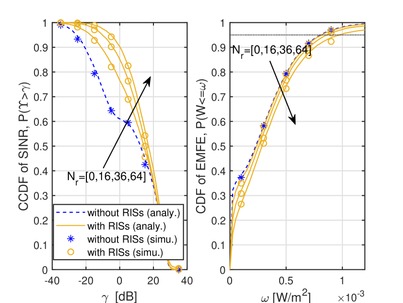
Figure 2: Marginal distributions of downlink SINR ($\Upsilon$) and EMFE ($\mathcal{W}$) for different values of the number of RIS elements ($N_{\rm r}$): coverage and compliance probabilities at $t_{\rm bu}=100~\rm m$.

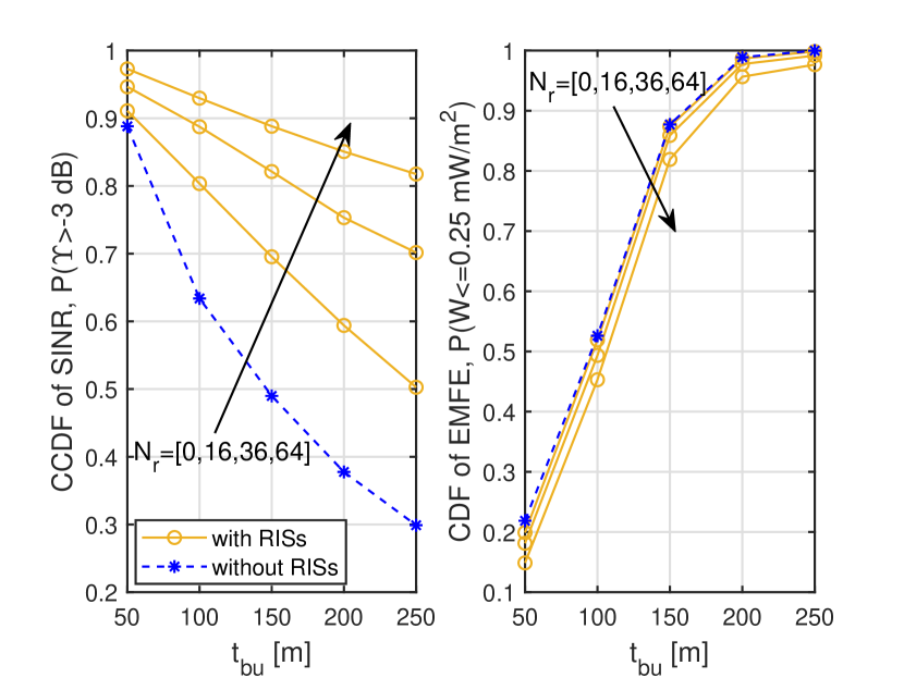
Figure 3: Impact of the BS-UE distance ($t_{\rm bu}$) on the marginal distributions of downlink SINR ($\Upsilon$) and EMFE ($\mathcal{W}$) at $\gamma=-3~\rm dB$ and $\omega=0.25~\rm mW/m^{2}$.

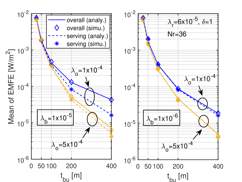
Figure 4: Mean of downlink EMFE caused by the serving signals and by the overall (serving and interfering) signals at different BS densities ($\lambda_{\rm b}$) and obstacle densities ($\lambda_{\rm o}$).

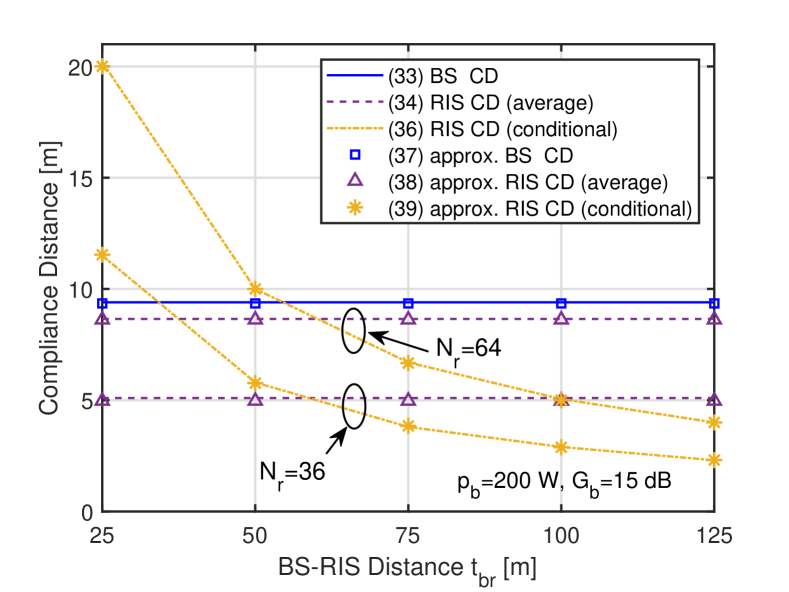
Figure 5: The conditional RIS CD $\hat{\tau}_{\rm ru}(t_{\rm br})$, the average RIS CD $\tau_{\rm ru}$, and the BS CD $\tau_{\rm bu}$ based on (33)-(36) and (37)-(39).

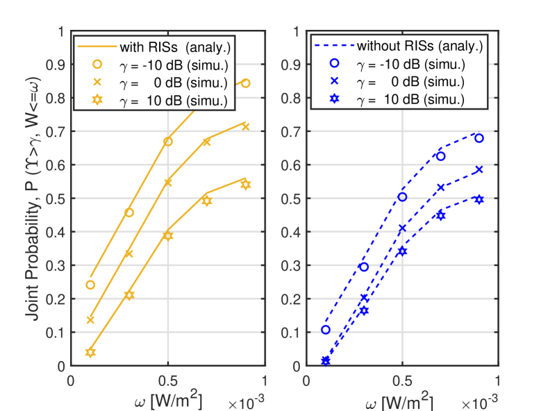
Figure 6: Joint distribution of downlink SINR and EMFE for different values of $\gamma$ and $\omega$ with RISs (left) and without RIS (right).

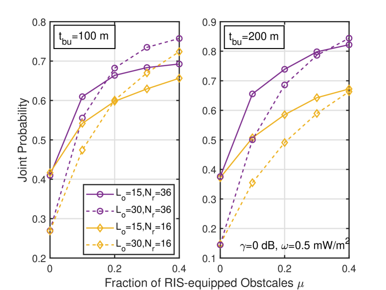
Figure 7: Joint metric on downlink SINR and EMFE for different values of $\mu$, $N_{\rm r}$, and $L_{\rm o}$ at $t_{\rm bu}=100~\rm m$ (left) and $t_{\rm bu}=200~\rm m$ (right).

Fig. 4 plots the CCDF of SINR (coverage probability) and the CDF of EMFE (compliance probability) in downlink for different values of the number of RIS elements ($N_{\rm r}$), where the curve of $N_{\rm r}=0$ refers to the network without RISs. The simulation results closely match the analytical results, which validates Theorems 1 and 2. Moreover, we see that deploying RISs significantly improves coverage performance, while slightly degrading compliance performance. For example, compared with the network without RISs, deploying RISs with $N_{\rm r}=64$ has roughly $40\%$ coverage enhancement at $\gamma=0~\rm dB$ and increases the 95-th percentile of EMFE from $0.8~\rm mW/m^{2}$ to $1~\rm mW/m^{2}$. The reason is that in the RIS-assisted network when the direct link between the typical user and its serving BS is NLoS, RISs can provide a LoS link with less attenuation than the NLoS link. Moreover, larger $N_{\rm r}$ provides higher RIS gain ($G_{\rm r}$) to compensate for the path loss in the cascaded (BS-RIS-user) link. This results in the increased received serving signal power and power density, thereby increasing SINR and EMFE.

Fig. 4 shows impact of the BS-UE distance ($t_{\rm bu}$) on the coverage probability and the compliance probability at $\gamma=-3~\rm dB$ and $\omega=0.25~\rm mW/m^{2}$ in downlink. The coverage probability gradually decreases with the increase of $t_{\rm bu}$ due to the increased path loss and NLoS probability of the serving link. For example, in the networks without RISs, the coverage probability is approximately $0.89$ when $t_{\rm bu}=50~\rm m$, whereas it drops to $0.3$ at $t_{\rm bu}=250~\rm m$. The small coverage range is a well-known challenge at millimeter wave (mmWave) communications ($f=28~\rm GHz$) [6]. Interestingly, exploiting RIS technologies can extend the coverage range. For example, to achieve a coverage probability greater than $0.8$ at $\gamma=-3~\rm dB$, $t_{\rm bu}$ should be less than roughly $75~\rm m$ at the network without RISs; whereas $t_{\rm bu}$ can increase to $100~\rm m$ at the RIS-assisted network with $N_{\rm r}=16$, and even to $250~\rm m$ at the network with RISs with $N_{\rm r}=64$. Moreover, we also see that when the typical user is closer to its serving BS, i.e., decreasing $t_{\rm bu}$, the compliance probability decreases in both networks with and without RISs. Therefore, to ensure the compliance probability is high enough for safety constraints, the minimum value of $t_{\rm bu}$ is worth consideration, which will be shown in the next subsection.

Fig. 4 presents mean values of downlink EMFE caused by serving signals and by overall (serving and interfering) signals, respectively. The close match between simulation and analytical results validates (32) in Theorem 2. From the left sub-figure, we see that the gap between EMFE caused by the serving signals and that caused by the overall signals gradually diminishes as the BS-UE distance $t_{\rm bu}$ shortens. This indicates that the received serving power density increasingly dominates EMFE at shorter distances, thereby justifying the reasonability of the approximation in Proposition 1. We observe that a higher obstacle density tends to reduce the overall EMFE since more interfering links are blocked. Additionally, a comparison between the left and right sub-figures reveals that a lower BS density also mitigates the overall EMFE by reducing the number of radiating sources. These findings collectively emphasize the dominant role of the received serving power density in EMFE in environments with short serving links, dense obstacles, or sparse BSs.

VII-A2 Compliance Distance (CD)

Fig. 7 presents the conditional RIS CD $\hat{\tau}_{\rm ru}$ (conditioned on BS-RIS distance $t_{\rm br}$), the average RIS CD $\tau_{\rm ru}$, and the BS CD $\tau_{\rm bu}$, under the conservative setting, where we consider the maximum transmit power ($200~\rm W$) and the maximum antenna gain ($15~\rm dB$) at BSs [23]. Specifically, $\hat{\tau}_{\rm ru}$, $\tau_{\rm ru}$, and $\tau_{\rm bu}$ are the minimum distances between a RIS/BS and a user to ensure that the 95-th percentile of EMFE remains within the safe limit $\mathcal{W}_{\max}$. Comparing the CDs based on (33)-(36) by the bi-sectional method with that based on (37)-(39) in Proposition 1, we verify the accuracy of the approximate expressions for CDs. Moreover, consistent with the observations from Proposition 1, we see that the conditional and average RIS CDs increases with $N_{\rm r}$. This is because increasing $N_{\rm r}$ exacerbates the EMFE level (as shown in Fig. 4), requiring a larger fence (i.e., a longer CD) around the RIS. Particularly, at $N_{\rm r}=64$, the average RIS CD is $\tau_{\rm ru}\approx 8~\rm m$, which is comparable to the BS CD $\tau_{\rm bu}\approx 9.5~\rm m$, implying that setting the RIS CD is as necessary as setting the BS CD. We also see that the conditional CD $\hat{\tau}_{\rm ru}$ is greater than the average CD $\tau_{\rm ru}$ at small values of BS-RIS distance $t_{\rm br}$; while $\hat{\tau}_{\rm ru}<\tau_{\rm ru}$ at large values of $t_{\rm br}$. Intuitively, when the RIS is closer to the BS, the path loss in the BS-RIS link significantly decreases, resulting in stronger incident and reflected power at the RIS. Therefore, the fence around the RIS should be enlarged to prevent users from entering areas with excessive EMFE.

VII-A3 Joint Probability

Fig. 7 shows the joint distribution of the downlink SINR ($\Upsilon$) and EMFE ($\mathcal{W}$), i.e., $\mathcal{J}_{\Upsilon,\mathcal{W}}(\gamma,\omega)$. We can see that the simulation results closely match the analytical results, which validates Theorem 3. Compared with the network without RISs, the RIS-assisted network has a higher probability of achieving a given SINR threshold $\gamma$ and adhering to a specified EMFE constraint level $\omega$ simultaneously. For example, under the constraint of SINR at $\gamma=0~\rm dB$, the probability that EMFE is less than $\omega=0.5~\rm mW/m^{2}$ is up to $0.55$ in the network with RISs, while only $0.4$ in the network without RISs. It can be concluded from Fig. 4 and 7 that the benefits of deploying RISs in enhancing coverage performance outweigh the compromises in EMFE compliance performance.

Fig. 7 shows the impact of the fraction of RIS-equipped obstacles $\mu$, the number of RIS elements $N_{\rm r}$, and the average length of obstacles $L_{\rm o}$ on the downlink performance at $\gamma=0\,\rm dB$ and $\omega=0.5\,\rm mW/m^{2}$. A larger $\mu$, i.e., a higher RIS density, increases the existence probability of the cascade LoS link in (19) and reduces the length of the cascade LoS link. Consequently, the received serving signal power and power density strengthen, positively impacting the SINR while negatively impacting the EMFE. We see that increasing $\mu$ improves system performance at $L_{\rm o}=15\,\rm m$ and $N_{\rm r}=16$, implying that the positive effect of increasing $\mu$ in coverage dominates. Interestingly, there is a different trend at low and high fractions of RISs-equipped obstacles as $L_{\rm o}$ increases. This is because the increased $L_{\rm o}$ not only decreases the LoS probability in the serving link but also in the interfering link, resulting in a decrease in both received power and the received power density in the serving link and the interfering link. The lowered received power density and reduced interference positively impact EMFE and SINR, while the decreased received power in the serving link negatively impacts SINR. For example, for $t_{\rm bu}=100~\rm m$, when $\mu\in[0,0.17)$, the detrimental impact of increasing $L_{\rm o}$ dominates, leading to performance degradation; contrarily, when $\mu\in(0.2,0.4]$, the density of RISs is sufficient to provide cascaded LoS links, compensating for the decreased LoS probability in the serving link. Thus, increasing $L_{\rm o}$ results in enhanced performance. These observations reveal the interdependence of the RIS deployment and the obstacle environment on the SINR and EMFE, providing valuable insights into RIS configuration to balance the trade-off between coverage and compliance performance.

VII-B Uplink Performance Evaluation

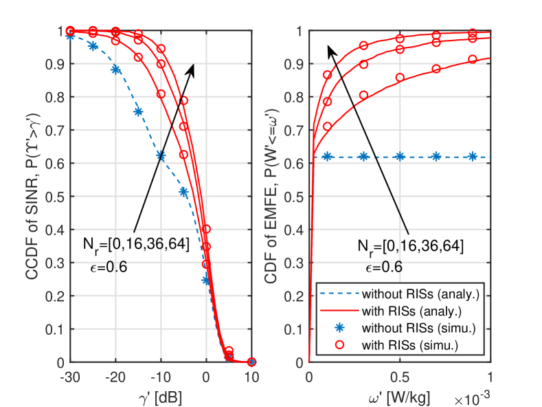
Figure 8: Marginal distributions of uplink SINR ($\Upsilon^{\prime}$) and EMFE ($\mathcal{W}^{\prime}$).

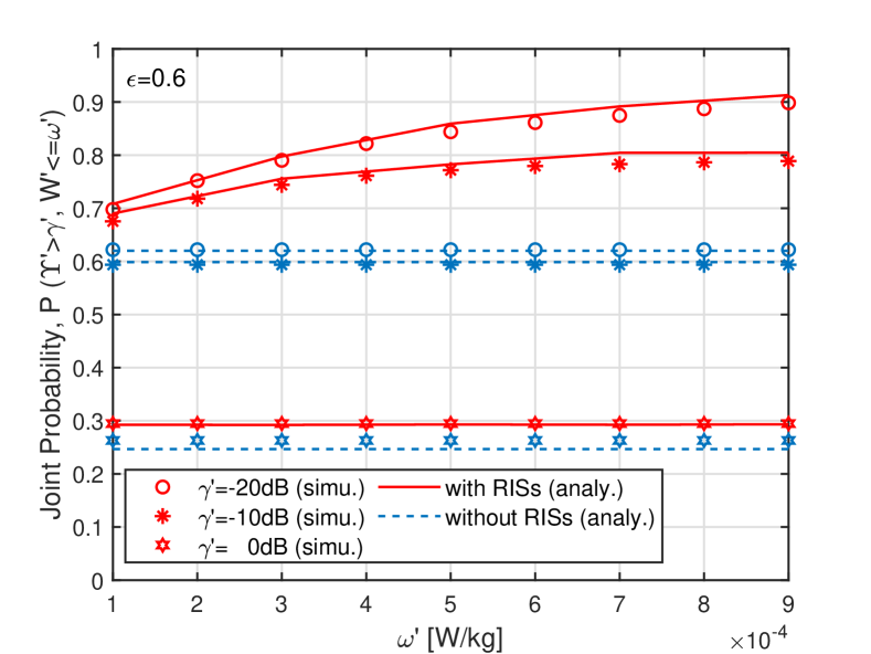
Figure 9: Joint distribution of uplink SINR and EMFE for different values of $\gamma^{\prime}$ and $\omega^{\prime}$.

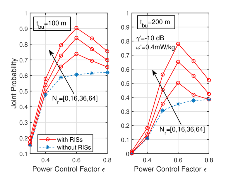
Figure 10: Joint metric on uplink SINR and EMFE for different power control factors $\epsilon$.

VII-B1 Marginal Probability

Fig. 10 plots the CCDF of SINR (coverage probability) and the CDF of EMFE (compliance probability) in the uplink for different values of $N_{\rm r}$. The simulation results closely match the analytical results, which validates Theorems 4 and 5. Additionally, it verifies the applicability of Lemma 5 in approximating the uplink interference. We see that in the network without RISs, the compliance probability is constant within $\omega^{\prime}\in[0.1,1]~\rm mW/kg$. This is because of the fixed BS-user distance $t_{\rm bu}$. From (60), the uplink compliance probability conditioned on $t_{\rm bu}$ in the direct LoS/NLoS link is either $0$ or $1$ at a given $\omega^{\prime}$. Thus, combining the association probability with the conditional compliance probability at a fixed $t_{\rm bu}$, the overall compliance probability is shown in the blue dashed curve at the right side of Fig. 10. Moreover, compared with the network without RISs, we see that deploying RISs with $N_{\rm r}=64$ not only improves the uplink coverage performance by roughly $43\%$ at $\gamma^{\prime}=-10~\rm dB$ but also improves the uplink compliance performance by roughly $43\%$ at $\omega^{\prime}=0.3~\rm mW/kg$. The reason behind the uplink coverage improvement is similar to that in the downlink case. The improvement in uplink compliance performance can be explained by the uplink power control mechanism in Sec. V-A1, which is different from the downlink case with constant transmit power. As indicated by (47), based on the power control factor $\epsilon$, RIS-assisted uplink transmission utilizes the RIS gain to partially compensate for path loss in the cascaded LoS link. With large enough $N_{\rm r}$ to provide high RIS gain, the transmit power in the cascaded LoS link can be reduced, mitigating the uplink EMFE.

VII-B2 Joint Probability

Fig. 10 shows the joint distribution of the uplink SINR ($\Upsilon^{\prime}$) and EMFE ($\mathcal{W}^{\prime}$), i.e., $\mathcal{J}_{\Upsilon^{\prime},\mathcal{W}^{\prime}}(\gamma^{\prime},\omega^{\prime})$. The high level of agreement between the simulation and analytical results confirms the validity of Theorem 6. We observe that for a given SINR threshold $\gamma^{\prime}=-10~\rm dB$, the probability that the uplink EMFE is below $\omega^{\prime}=0.4~\rm mW/kg$ increases by roughly $15\%$ after deploying $16$-element RISs. This observation aligns with the insights from Fig. 10, which shows deploying RISs is effective in increasing uplink SINR and mitigating uplink EMFE. Therefore, it can be expected that deploying RISs improves joint coverage and compliance performance in the uplink. Moreover, the gap between the joint probability in the network with and without RISs is small at the high SINR threshold $\gamma^{\prime}=0~\rm dB$. This can be explained by Fig. 10. Specifically, deploying $16$-element RISs slightly increases the coverage probability at $0~\rm dB$. Moreover, the probability that the SINR is greater than $0~\rm dB$ is quite small, which dominantly influences the joint distribution of SINR and EMFE in the high SINR regime. Therefore, the joint probability at $\gamma^{\prime}=0~\rm dB$ slightly increases by deploying RISs.

Fig. 10 shows the impact of the power control factor $\epsilon$ on the uplink joint performance at $\gamma^{\prime}=-10\,\rm dB$ and $\omega^{\prime}=0.4\,\rm mW/kg$. With an increase in $\epsilon$, the uplink exposure (measured by the transmit power of the typical user) intensifies. This is because the transmit power of a user is proportional to $\epsilon$, as shown in (45)-(47). Moreover, the increased transmit power strengthens the serving signal power while the interference from interfering users also increases. Under the default values of system parameters given in Table II, we find a trade-off value of $\epsilon$ at $0.6$ for the RIS-assisted networks, which provides the optimal balance between the benefits of increased serving signal power and the negative impact of increased EMFE and interference. The finding emphasizes the importance of the power control factor in designing and optimizing RIS-assisted networks.

VIII Conclusions

This paper provides a framework for modeling RIS-assisted networks for the downlink and uplink and for analyzing the impact of RIS deployment on both SINR and EMFE independent or jointly. From the numerical results, both the downlink and uplink joint distributions show that the RIS-assisted network has better performance than the network without RISs. Specifically, after deploying $16$-element RISs, the joint performance increases by roughly $15\%$ at given thresholds $\gamma=0~\rm dB$ and $\omega=0.5~\rm mW/m^{2}$ in downlink (or $\gamma^{\prime}=-10~\rm dB$ and $\omega^{\prime}=0.4~\rm mW/kg$ in uplink). These affirm the feasibility of the RIS deployment. However, to further enable the practical deployment, it is crucial to consider EMFE regulations tailored to RIS as the marginal distribution indicates a higher downlink EMFE with RIS deployment. For example, for the CD design, when the distance between a $64$-element RIS and a BS is as close as only $25~\rm m$, users should be strictly prohibited from entering the area centered at the RIS with a radius of $20~\rm m$ because of the excessive EMFE within this area. Moreover, the adjustable parameters (e.g., the densities and the sizes of antennas and RISs, and the power control factor) enable the performance evaluation of different configurations of RIS-assisted networks. For example, we find a trade-off value of the power control factor, which maximizes the joint uplink performance under a specific network configuration. Overall, our study sheds light on RIS deployment strategies to strike a balance between SINR enhancement and EMFE management.

For future works, it would be interesting to extend the proposed framework to different types of RISs, e.g., simultaneously transmitting and reflecting (STAR)-RIS [51]. Moreover, beam misalignment, which could potentially affect SINR adversely and EMFE favorably, is also a future research direction. Fully understanding the impact of beam misalignment caused by, e.g., the fixed codebook with finite directional beams and the imperfect channel angle information, could provide valuable insights into determining optimal codebook size and the precision required for channel estimation.

Appendix A Proof of Lemma 3

The Laplace transform of $I_{\rm B}$ conditioned on $t_{\rm bu}$ is

$$\mathcal{L}_{I_{\rm B}|t_{\rm bu}}(s) =\mathbb{E}\left[\exp\left(-sI_{\rm B}\right)\right]=\mathbb{E}\left[\exp\left(-s(I_{\rm b,L}+I_{\rm b,N})\right)\right]$$

$$=\prod_{v\in\{\rm L,N\}}\mathbb{E}_{\Psi_{{\rm b},v},H_{v,i}}\left[\exp\left(-sI_{{\rm b},v}\right)\right].$$ (63)

Define $\mathcal{L}_{I_{{\rm b},v}|t_{\rm bu}}(s)=\mathbb{E}_{\Psi_{{\rm b},v},H_{v,i}}\left[\exp\left(-sI_{{\rm b},v}\right)\right]$. Then,

$$\mathcal{L}_{I_{{\rm b},v}|t_{\rm bu}}(s)$$

$$=\mathbb{E}_{\Psi_{{\rm b},v},H_{v,i}}\left[\exp\left(-s\!\!\!\!\!\!\sum_{i,\mathbf{b}_{i}\in\Psi_{{\rm b},v}\setminus\{\mathbf{b}_{0}\}}\!\!\!\!\!\!{p_{\rm b}G_{\rm B}(\Delta_{i})\zeta d_{i}^{-\alpha_{v}}H_{v,i}}\right)\right]$$

$$=\mathbb{E}_{\Psi_{{\rm b},v}}\left[\prod_{i,\mathbf{b}_{i}\in\Psi_{{\rm b},v}\setminus\{\mathbf{b}_{0}\}}\!\!\!\!\!\!\mathbb{E}_{H_{v,i}}[\exp\left(-s{p_{\rm b}G_{\rm B}(\Delta_{i})\zeta d_{i}^{-\alpha_{v}}H_{v,i}}]\right)\right]$$

$$\overset{(a)}{=}\mathbb{E}_{\Psi_{{\rm b},v}}\left[\prod_{i,\mathbf{b}_{i}\in\Psi_{{\rm b},v}\setminus\{\mathbf{b}_{0}\}}\left(\frac{m_{v}}{m_{v}+sp_{\rm b}G_{\rm B}(\Delta_{i})\zeta d_{i}^{-\alpha_{v}}}\right)^{m_{v}}\right]$$

$$\overset{(b)}{=}\exp\bigg{(}-2\pi\lambda_{\rm b}\int_{t_{\rm bu}}^{\infty}[1-\hat{\kappa}_{v}(d_{i})]d_{i}\mathcal{P}_{v}(d_{i})\mathrm{d}d_{i}\bigg{)},$$ (64)

where $\hat{\kappa}_{v}(d_{i})=\mathbb{E}_{\Delta_{i}}\left[\left(1+\frac{sp_{\rm b}G_{\rm B}(\Delta_{i})\zeta}{m_{v}d_{i}^{\alpha_{v}}}\right)^{-m_{v}}\right]$, (a) is from the PDF of small-scale fading coefficient $H_{v,i}$ in (5), and (b) is from the probability generating functional (PGFL) of the PPP [16] with the density of $\Psi_{{\rm b},v}$ being $\lambda_{\rm b}\mathcal{P}_{v}(d_{i})$. Based on $f_{\Delta}(\cdot)$ in (21), we can further express $\hat{\kappa}_{v}(d_{i})$ as

$$\begin{split}\hat{\kappa}_{v}(d_{i})&=\int_{-1}^{1}\!\!\left(1+\frac{sp_{\rm b}G_{\rm B}(\Delta_{i})\zeta}{m_{v}d_{i}^{\alpha_{v}}}\right)^{-m_{v}}f_{\Delta}(\Delta_{i})\mathrm{d}\Delta_{i}\\ &\overset{(a)}{=}\sum_{n=0}^{\tilde{N}_{\rm b}+1}p_{n}\left(1+\frac{sp_{\rm b}G_{n}\zeta}{m_{v}d_{i}^{\alpha_{v}}}\right)^{-m_{v}},\end{split}$$ (65)

where $p_{n}$ is given in (22) and (a) is from Lemma 1. Substituting (65) and (A) into (A), we finish the proof.

Appendix B Proof of Theorem 2

The CDF of the overall EMFE $\mathcal{W}$ can be derived based on the conditional compliance probability in (IV-E). The first moment of $\mathcal{W}$ is defined as

$$\begin{split}&\mathbb{E}[\mathcal{W}]=\mathbb{E}\bigg{[}\sum_{q\in\mathcal{S}}{\mathcal{W}_{q}}\mathcal{A}_{q}\bigg{]}\overset{(a)}{=}\mathbb{E}\bigg{[}\sum_{q\in\mathcal{S}}\mathcal{W}_{1,q}\mathcal{A}_{q}+\mathcal{W}_{2}\bigg{]}\\ &\overset{(b)}{=}\mathbb{E}\bigg{[}\sum_{q\in\mathcal{S}}\mathcal{W}_{1,q}\mathcal{A}_{q}+\mathcal{W}_{\rm b,L}+\mathcal{W}_{\rm b,N}\bigg{]}\\ &=\mathbb{E}_{t_{\rm bu},t_{\rm ru},t_{\rm br}}\bigg{[}\sum_{q\in\mathcal{S}}\mathcal{A}_{q}\mathbb{E}_{H_{q}}[\mathcal{W}_{1,q}]\bigg{]}+\\ &~\quad\mathbb{E}_{t_{\rm bu}}\bigg{[}\mathbb{E}_{\Psi_{{\rm b,L}},\phi_{i},H_{{\rm L},i}}[\mathcal{W}_{\rm b,L}]+\mathbb{E}_{\Psi_{{\rm b,N}},\phi_{i},H_{{\rm N},i}}[\mathcal{W}_{\rm b,N}]\bigg{]},\end{split}$$ (66)

where (a) is from (14), and (b) is from (13). With (12) and $\mathbb{E}[H_{q}]=1$, we have

$$\mathbb{E}_{H_{q}}[\mathcal{W}_{1,q}]=\mathbb{E}_{H_{q}}\bigg{[}{P^{\rm a}_{q}H_{q}}{\mathcal{E}^{-1}}\bigg{]}={P^{\rm a}_{q}}{\mathcal{E}^{-1}}.$$ (67)

From (13), (8), and ${\mathcal{E}}/{\zeta}=4\pi$, we have

$$\mathbb{E}_{\Psi_{{\rm b,L}},\Delta_{i},H_{{\rm L},i}}[\mathcal{W}_{\rm b,L}]$$

$$=\mathbb{E}_{\Psi_{{\rm b,L}},\Delta_{i},H_{{\rm L},i}}\bigg{[}\sum_{i,\mathbf{b}_{i}\in\Psi_{{\rm b,L}}\setminus\{\mathbf{b}_{0}\}}\!\!\!\!\frac{p_{\rm b}G_{\rm B}(\Delta_{i})H_{{\rm L},i}}{4\pi d_{i}^{\alpha_{\rm L}}}\bigg{]}$$

$$\overset{(a)}{=}\int_{t_{\rm bu}}^{\infty}\mathbb{E}_{\Delta_{i},H_{{\rm L},i}}\bigg{[}\frac{p_{\rm b}G_{\rm B}(\Delta_{i})H_{{\rm L},i}}{4\pi d_{i}^{\alpha_{\rm L}}}\bigg{]}2\pi\lambda_{\rm b}\mathcal{P}_{\rm L}(d_{i})d_{i}\mathrm{d}d_{i}$$

$$=\int_{t_{\rm bu}}^{\infty}\frac{p_{\rm b}\mathbb{E}_{\Delta}[G_{\rm B}(\Delta)]\mathbb{E}[H_{{\rm L}}]}{2d_{i}^{\alpha_{\rm L}}}\lambda_{\rm b}\mathcal{P}_{\rm L}(d_{i})d_{i}\mathrm{d}d_{i}$$

$$\overset{(b)}{=}\frac{\lambda_{\rm b}p_{\rm b}\bar{g}_{\rm B}}{2}\int_{t_{\rm bu}}^{\infty}\frac{\exp\left(-\beta t\right)}{t^{\alpha_{\rm L}-1}}\mathrm{d}t,$$ (68)

where (a) applies Campbell Theorem [15] with the density of $\Psi_{{\rm b,L}}$ being $\lambda_{\rm b}\mathcal{P}_{\rm L}(d_{i})$, (b) replaces $d_{i}$ with $t$, (b) is also from $\mathcal{P}_{\rm L}(t)$ in (4), $\mathbb{E}[H_{{\rm L}}]=1$, and $\bar{g}_{\rm B}=\mathbb{E}_{\Delta}[G_{\rm B}(\Delta)]=\sum_{n=0}^{\tilde{N}_{\rm b}}G_{n}p_{n}$ is from Lemma 1, Similarly, considering that the density of $\Psi_{{\rm b,N}}$ is $\lambda_{\rm b}\mathcal{P}_{\rm N}(d_{i})=\lambda_{\rm b}(1-\mathcal{P}_{\rm L}(d_{i}))$, we have

$$\mathbb{E}_{\Psi_{{\rm b,N}},\Delta_{i},H_{{\rm N},i}}[\mathcal{W}_{\rm b,N}]=\frac{\lambda_{\rm b}p_{\rm b}\bar{g}_{\rm B}}{2}\!\!\int_{t_{\rm bu}}^{\infty}\frac{1-\exp\left(-\beta t\right)}{t^{\alpha_{\rm N}-1}}\mathrm{d}t.$$ (69)

Note that $\int_{a}^{\infty}\frac{\exp\left(-\beta t\right)}{t^{n}}\mathrm{d}t=a^{1-n}{\rm E}_{n}(\beta a)$, and ${\rm E}_{n}(x)=\int_{1}^{\infty}\frac{\exp\left(-xt\right)}{t^{n}}\mathrm{d}t$. Substituting (67)-(69) into (66), we prove (32).

Appendix C Proof of Proposition 1

From (14) and (IV-E), considering the dominant downlink EMFE from the serving link, we approximate the BS CD in (33) as

$$\begin{split}\tau_{\rm bu}&=\inf_{t_{\rm bu}\in\mathbb{R}}\left\{t_{\rm bu}:\mathbb{P}(\mathcal{W}_{1,\rm DL}+\mathcal{W}_{2}\leq\mathcal{W}_{\max}|t_{\rm bu})\geq\rho\right\}\\ &\approx\inf_{t_{\rm bu}\in\mathbb{R}}\left\{t_{\rm bu}:\mathbb{P}(\mathcal{W}_{1,\rm DL}|t_{\rm bu}\leq\mathcal{W}_{\max}|t_{\rm bu})\geq\rho\right\}\\ &\triangleq\inf_{t_{\rm bu}\in\mathbb{R}}\left\{t_{\rm bu}:F_{\mathcal{W}_{1,\rm DL}|t_{\rm bu}}(\mathcal{W}_{\max})\geq\rho\right\}.\end{split}$$ (70)

From (12), we have

$$F_{\mathcal{W}_{1,\rm DL}|t_{\rm bu}}(\omega) =\mathbb{P}(\mathcal{W}_{1,\rm DL}\leq\omega|t_{\rm bu})=\mathbb{P}\bigg{(}\frac{P^{\rm a}_{\rm DL}H_{\rm DL}}{\mathcal{E}}\leq\omega|t_{\rm bu}\bigg{)}$$

$$=\mathbb{P}\bigg{(}H_{\rm DL}\leq\frac{\mathcal{E}\omega}{P^{\rm a}_{\rm DL}}|t_{\rm bu}\bigg{)}=F_{H_{\rm L}}\bigg{(}\frac{\mathcal{E}\omega}{P^{\rm a}_{\rm DL}}\bigg{)},$$ (71)

where $F_{H_{\rm L}}(\cdot)$ is the PDF of $H_{\rm DL}$ given in (5a) and $P^{\rm a}_{\rm DL}$ is given in (6). With (C) and (6), (70) can be further expressed as

$$\begin{split}\tau_{\rm bu}&\approx\inf_{t_{\rm bu}\in\mathbb{R}}\left\{t_{\rm bu}:F_{H_{\rm L}}\bigg{(}\frac{\mathcal{E}\mathcal{W}_{\max}}{p_{\rm b}G_{\rm b}\zeta t_{\rm bu}^{-\alpha_{\rm L}}}\bigg{)}\geq\rho\right\}\\ &=\bigg{(}\frac{p_{\rm b}G_{\rm b}\zeta}{\mathcal{E}\mathcal{W}_{\max}}F_{H_{\rm L}}^{-1}(\rho)\bigg{)}^{\frac{1}{\alpha_{\rm L}}}\!\!\!\!=\!\!\bigg{(}\frac{p_{\rm b}G_{\rm b}}{4\pi\mathcal{W}_{\max}}F_{H_{\rm L}}^{-1}(\rho)\bigg{)}^{\frac{1}{\alpha_{\rm L}}}.\end{split}$$ (72)

Similar to (C), we define the CDF of the EMFE from the cascaded LoS link as

$$F_{\mathcal{W}_{1,\rm CL}|t_{\rm ru},t_{\rm br}}(\omega) =\mathbb{P}(\mathcal{W}_{1,\rm CL}\leq\omega|t_{\rm ru},t_{\rm br})=F_{H_{\rm L}}\bigg{(}\frac{\mathcal{E}\omega}{P^{\rm a}_{\rm CL}}\bigg{)},$$

where $P^{\rm a}_{\rm CL}$ is given in (7). Then, we approximate the conditional RIS CD in (36) as

$$\hat{\tau}_{\rm ru}(t_{\rm br}) \approx\inf_{t_{\rm ru}\in\mathbb{R}}\left\{t_{\rm ru}:F_{\mathcal{W}_{1,\rm CL}|t_{\rm ru},t_{\rm br}}(\mathcal{W}_{\max})\geq\rho\right\}$$

$$=\bigg{(}\frac{p_{\rm b}G_{\rm b}G_{\rm r}t_{\rm br}^{-\alpha_{\rm L}}}{4\pi\mathcal{W}_{\max}}F_{H_{\rm L}}^{-1}(\rho)\bigg{)}^{\frac{1}{\alpha_{\rm L}}}.$$ (73)

Similarly, for the average RIS CD,

$$\begin{split}\tau_{\rm ru}&\approx\inf_{t_{\rm ru}\in\mathbb{R}}\left\{t_{\rm ru}:\mathbb{E}_{t_{\rm br}}[F_{\mathcal{W}_{1,\rm CL}|t_{\rm ru},t_{\rm br}}(\mathcal{W}_{\max})]\geq\rho\right\}.\end{split}$$ (74)

The approximation in (74) implies that $\tau_{\rm ru}$ satisfies

$$\mathbb{E}_{t_{\rm br}}\bigg{[}F_{H_{\rm L}}\bigg{(}\frac{4\pi\mathcal{W}_{\max}}{p_{\rm b}G_{\rm b}G_{\rm r}(\tau_{\rm ru}t_{\rm br})^{-\alpha_{\rm L}}}\bigg{)}\bigg{]}=\rho.$$ (75)

In (74) and (75), given $t_{\rm ru}$, we observe from (1) that $t_{\rm br}$ is a random variable whose distribution depends on $t_{\rm bu}$ and $\theta_{0}$. This greatly complicates the calculation of $\mathbb{E}_{t_{\rm br}}[F_{H_{\rm L}}(h_{0}t_{\rm br}^{\alpha_{\rm L}})]$, where

$$h_{0}={4\pi\mathcal{W}_{\max}}{(p_{\rm b}G_{\rm b}G_{\rm r}\tau_{\rm ru}^{-\alpha_{\rm L}})^{-1}}.$$ (76)

To simplify the calculation of $\mathbb{E}_{t_{\rm br}}[\cdot]$ , we notice that $t_{\rm br}$ satisfies the triangle inequality $|t_{\rm bu}-t_{\rm ru}|\leq t_{\rm br}\leq t_{\rm bu}+t_{\rm ru}$. Considering that the value of $\tau_{\rm ru}$ is generally small, when $t_{\rm ru}=\tau_{\rm ru}$, we can expect that $t_{\rm br}\approx t_{\rm bu}$. Inspired by this, we use the PDF of $t_{\rm bu}$, i.e., $f_{T_{\rm bu}}(\cdot)$ in (23), to approximate the distribution of $t_{\rm br}$. Then, $\mathbb{E}_{t_{\rm br}}[F_{H_{\rm L}}(h_{0}t_{\rm br}^{\alpha_{\rm L}})]$ in (75) becomes

$$\mathbb{E}_{t_{\rm br}}[F_{H_{\rm L}}(h_{0}t_{\rm br}^{\alpha_{\rm L}})]\overset{(a)}{\approx}\int_{0}^{\infty}F_{H_{\rm L}}(h_{0}t_{\rm br}^{\alpha_{\rm L}})f_{T_{\rm bu}}(t_{\rm br})\mathrm{d}t_{\rm br}$$

$$\overset{(b)}{=}\int_{0}^{\infty}\frac{\Gamma_{l}(m_{\rm L},m_{\rm L}h_{0}t^{\alpha_{\rm L}})}{\Gamma(m_{\rm L})}2\pi\lambda_{\rm b}t\exp(-\pi\lambda_{\rm b}t^{2})\mathrm{d}t$$

$$\overset{(c)}{=}-\frac{\Gamma_{l}(m_{\rm L},m_{\rm L}h_{0}t^{\alpha_{\rm L}})}{\Gamma(m_{\rm L})}\exp(-\pi\lambda_{\rm b}t^{2})\bigg{|}_{0}^{\infty}+$$

$$\qquad\int_{0}^{\infty}\exp(-\pi\lambda_{\rm b}t^{2})\mathrm{d}\frac{\Gamma_{l}(m_{\rm L},m_{\rm L}h_{0}t^{\alpha_{\rm L}})}{\Gamma(m_{\rm L})}$$

$$\overset{(d)}{=}\frac{\alpha_{\rm L}(m_{\rm L}h_{0})^{m_{\rm L}}}{\Gamma(m_{\rm L})}\!\!\int_{0}^{\infty}\!\!t^{m_{\rm L}\alpha_{\rm L}-1}e^{-m_{\rm L}h_{0}t^{\alpha_{\rm L}}-\pi\lambda_{\rm b}t^{2}}\mathrm{d}t$$

$$\triangleq F_{\alpha_{\rm L}}(h_{0}),$$ (77)

where (a) is from $t_{\rm br}\approx t_{\rm bu}$ when $t_{\rm ru}=\tau_{\rm ru}$ is small, (b) replaces $t_{\rm br}$ with $t$, (b) is also from (5a) and (23), (c) is from integration by parts, (d) is from $\mathrm{d}\Gamma_{l}(m,x)=\mathrm{d}\int_{0}^{x}z^{m-1}e^{-z}\mathrm{d}z=x^{m-1}e^{-x}$. From (C) and (75), we have $h_{0}=F_{\alpha_{\rm L}}^{-1}(\rho)$, where $F_{\alpha_{\rm L}}^{-1}(\rho)$ is the inverse function of $F_{\alpha_{\rm L}}(h_{0})$. Then, with (76), we obtain (39). Furthermore, when $\alpha_{\rm L}=2$, we obtain

$$F_{\alpha_{\rm L}=2}(h_{0}) =\frac{2(m_{\rm L}h_{0})^{m_{\rm L}}}{\Gamma(m_{\rm L})}\int_{0}^{\infty}t^{2m_{\rm L}-1}e^{-(m_{\rm L}h_{0}+\pi\lambda_{\rm b})t^{2}}\mathrm{d}t$$

$$\overset{(a)}{=}\frac{(m_{\rm L}h_{0})^{m_{\rm L}}}{\Gamma(m_{\rm L})}\int_{0}^{\infty}z^{m_{\rm L}-1}e^{-(m_{\rm L}h_{0}+\pi\lambda_{\rm b})z}\mathrm{d}z$$

$$\overset{(b)}{=}\frac{(m_{\rm L}h_{0})^{m_{\rm L}}}{\Gamma(m_{\rm L})(m_{\rm L}h_{0}+\pi\lambda_{\rm b})^{m_{\rm L}}}\int_{0}^{\infty}x^{m_{\rm L}-1}e^{-x}\mathrm{d}x$$

$$\overset{(c)}{=}{(m_{\rm L}h_{0})^{m_{\rm L}}}{(m_{\rm L}h_{0}+\pi\lambda_{\rm b})^{-m_{\rm L}}},$$ (78)

where (a) replaces $t^{2}$ with $z$, (b) replaces $(m_{\rm L}h_{0}+\pi\lambda_{\rm b})z$ with $x$, and (c) is from $\Gamma(m)=\int_{0}^{\infty}x^{m-1}e^{-x}\mathrm{d}x$. Then, $F_{\alpha_{\rm L}=2}(h_{0})=\rho$ implies that

$$\begin{split}h_{0}=\frac{\pi\lambda_{\rm b}\rho^{\frac{1}{m_{\rm L}}}}{m_{\rm L}\big{(}1-\rho^{\frac{1}{m_{\rm L}}}\big{)}}~{\rm for}~\alpha_{\rm L}=2.\end{split}$$ (79)

Substituting (79) into (76), we obtain (41).

Appendix D Proof of Theorem 3

Certain techniques for deriving the joint metric have been explored in [28, 30, 29], which can be adapted for deriving Theorem 3 in our work. Specifically, when the serving link is direct LoS, the downlink joint probability conditioned on $t_{\rm bu}$ is

$$J_{\Upsilon_{\rm DL},\mathcal{W}_{\rm DL}|t_{\rm bu}}(\gamma,\omega)=\mathbb{P}({\Upsilon_{\rm DL}}>\gamma,{\rm\mathcal{W}_{\rm DL}}\leq\omega|t_{\rm bu})$$

$$\overset{(a)}{=}\mathbb{P}(\frac{P_{\rm DL}}{\sigma^{2}+I_{\rm B}}>\gamma,\frac{P_{\rm DL}+I_{\rm B}}{\mathcal{E}}\leq\omega)$$

$$\overset{(b)}{=}\mathbbm{1}(\mathcal{E}\omega-\sigma^{2}\gamma\geq 0)\mathbb{P}(I_{\rm B}<\frac{P_{\rm DL}}{\gamma}-\sigma^{2},I_{\rm B}\leq\mathcal{E}\omega-P_{\rm DL})$$

$$\overset{(c)}{=}\mathbbm{1}(\mathcal{E}\omega-\sigma^{2}\gamma\geq 0)\times$$

$$\quad\begin{cases}\mathbb{P}(I_{\rm B}<\frac{P_{\rm DL}}{\gamma}-\sigma^{2}),&\text{ if }\sigma^{2}\gamma\leq P_{\rm DL}<P_{1},\\ \mathbb{P}(I_{\rm B}\leq\mathcal{E}\omega-P_{\rm DL}),&\text{ if }P_{1}\leq P_{\rm DL}<\mathcal{E}\omega,\\ 0,&\text{ otherwise,}\end{cases}$$ (80)

where $P_{1}=\frac{\gamma(\mathcal{E}\omega+\sigma^{2})}{1+\gamma}$, (a) is from (14), and (b) and (c) is from the non-negativity of interference (i.e., $I_{\rm B}\geq 0$) [29]. Specifically, either $P_{\rm DL}<\sigma^{2}\gamma$ or $P_{\rm DL}>\mathcal{E}\omega$ leads to $I_{\rm B}<0$. Therefore, when $\mathcal{E}\omega<\sigma^{2}\gamma$, $J_{\Upsilon_{\rm DL},\mathcal{W}_{\rm DL}|t_{\rm bu}}(\gamma,\omega)=0$. Moreover, when $\mathcal{E}\omega\geq\sigma^{2}\gamma$, $\sigma^{2}\gamma\leq P_{1}<\mathcal{E}\omega$. Let $U(\gamma,\omega)=\mathbbm{1}(\mathcal{E}\omega-\sigma^{2}\gamma\geq 0)$. Substituting (6) into (D), we have

$$J_{\Upsilon_{\rm DL},\mathcal{W}_{\rm DL}|t_{\rm bu}}(\gamma,\omega)=U(\gamma,\omega)\times$$

$$\Bigg{(}\mathbb{E}\left[\mathbbm{1}(\frac{\sigma^{2}\gamma}{P^{\rm a}_{\rm DL}}\leq H_{\rm DL}<\frac{P_{1}}{P^{\rm a}_{\rm DL}})\mathbb{P}(I_{\rm B}<\frac{P^{\rm a}_{\rm DL}H_{\rm DL}}{\gamma}-\sigma^{2})\right]$$

$$~+\mathbb{E}\left[\mathbbm{1}(\frac{P_{1}}{P^{\rm a}_{\rm DL}}\leq H_{\rm DL}<\frac{\mathcal{E}\omega}{P^{\rm a}_{\rm DL}})\mathbb{P}(I_{\rm B}<\mathcal{E}\omega-P^{\rm a}_{\rm DL}H_{\rm DL})\right]\Bigg{)}$$

$$=U(\gamma,\omega)\times\Bigg{(}\underbrace{\int_{\frac{\sigma^{2}\gamma}{P^{\rm a}_{\rm DL}}}^{\frac{P_{1}}{P^{\rm a}_{\rm DL}}}F_{I_{\rm B}|t_{\rm bu}}\bigg{(}\frac{P^{\rm a}_{\rm DL}h}{\gamma}-\sigma^{2}\bigg{)}f_{H_{\rm L}}(h)\mathrm{d}h}_{\mathcal{J}^{\rm DL}_{1}}$$

$$~+\underbrace{\int^{\frac{\mathcal{E}\omega}{P^{\rm a}_{\rm DL}}}_{\frac{P_{1}}{P^{\rm a}_{\rm DL}}}F_{I_{\rm B}|t_{\rm bu}}\bigg{(}\mathcal{E}\omega-P^{\rm a}_{\rm DL}h\bigg{)}f_{H_{\rm L}}(h)\mathrm{d}h}_{\mathcal{J}^{\rm DL}_{2}}\Bigg{)},$$ (81)

where $F_{I_{\rm B}|t_{\rm bu}}(p)=\mathbb{P}(I_{\rm B}\leq p|t_{\rm bu})$ is the CDF of $I_{\rm B}$ conditioned on $t_{\rm bu}$ and $f_{H_{\rm L}}(h)$ is the PDF of $H_{\rm DL}$ given in (5). It is worth noting that for a continuous variable $H$, the CDF of $H$ is $F_{H}(h)=\mathbb{P}(H\leq h)=\mathbb{P}(H<h)$. Therefore, the replacement between “$<$” and “$\leq$” in (D) does not affect the results. In the following, we derive $F_{I_{\rm B}|t_{\rm bu}}(p)$ and $f_{H_{\rm L}}(h)$ to obtain the final expression of (D). From Gil-Pelaez theorem, the CDF of $I_{\rm B}$ is

$$\begin{split}F_{I_{\rm B}|t_{\rm bu}}(p)&=\frac{1}{2}-\int_{0}^{\infty}\frac{1}{\pi x}{\rm Im}\left[e^{-jxp}\mathcal{L}_{I_{\rm B}|t_{\rm bu}}(-jx)\right]{\rm d}x,\end{split}$$ (82)

where $\mathcal{L}_{I_{\rm B}|t_{\rm bu}}(\cdot)$ is given in (A). By noting that shaping parameter $m_{\rm L}$ is an integer, the CDF of $H_{\rm DL}$ in (5) can be further expressed as

$$F_{H_{\rm L}}(h)\overset{(a)}{=}1-\frac{\Gamma_{u}(m_{\rm L},m_{\rm L}h)}{\Gamma(m_{\rm L})}\overset{(b)}{=}1-e^{-m_{\rm L}h}\sum_{k=0}^{m_{\rm L}-1}\frac{(m_{\rm L}h)^{k}}{k!},$$ (83)

where $\Gamma_{u}\left(m,mg\right)=\int_{mg}^{\infty}x^{m-1}e^{-x}\mathrm{d}x$, (a) is from $\Gamma_{l}\left(m,mg\right)=\Gamma\left(m\right)-\Gamma_{u}\left(m,mg\right)$, and (b) is from the fact that $\frac{\Gamma_{u}\left(m,g\right)}{\Gamma\left(m\right)}=\exp(-g){\textstyle\sum_{k=0}^{m-1}}\frac{g^{k}}{k!}$ for $m\in\mathbb{N}$. Then, we can obtain the PDF of $H_{\rm DL}$ as $f_{H_{\rm L}}(h)=\frac{\mathrm{d}F_{H_{\rm L}}(h)}{\mathrm{d}h}$, i.e.,

$$f_{H_{\rm L}}(h)=-\!\!\!\sum_{k=0}^{m_{\rm L}-1}\frac{m_{\rm L}^{k}}{k!}\left(-m_{\rm L}e^{-m_{\rm L}h}h^{k}+ke^{-m_{\rm L}h}h^{k-1}\right).$$ (84)

Substituting (82)-(84) into $\mathcal{J}^{\rm DL}_{1}$, we have

$$\mathcal{J}^{\rm DL}_{1}=\frac{1}{2}F_{H_{\rm L}}\bigg{(}\frac{P_{1}}{P^{\rm a}_{\rm DL}}\bigg{)}-\frac{1}{2}F_{H_{\rm L}}\bigg{(}\frac{\sigma^{2}\gamma}{P^{\rm a}_{\rm DL}}\bigg{)}-$$

$$\quad\int_{0}^{\infty}\frac{1}{\pi x}{\rm Im}\left[\Xi^{\rm DL}_{1}(-jx)\exp(jx\sigma^{2})\mathcal{L}_{I_{\rm B}|t_{\rm bu}}(-jx)\right]{\rm d}x,$$ (85)

where $\Xi^{\rm DL}_{1}(-jx)=\int_{\frac{\sigma^{2}\gamma}{P^{\rm a}_{\rm DL}}}^{\frac{P_{1}}{P^{\rm a}_{\rm DL}}}\exp\left(-jx\frac{P^{\rm a}_{\rm DL}h}{\gamma}\right)f_{H_{\rm L}}(h)\mathrm{d}h$. Substituting (84) into $\Xi^{\rm DL}_{1}(-jx)$, we have

$$\Xi^{\rm DL}_{1}(-jx)=\exp\left(-jx\frac{P^{\rm a}_{\rm DL}h}{\gamma}\right)(F_{H_{\rm L}}(h)-1)\bigg{|}_{\frac{\sigma^{2}\gamma}{P^{\rm a}_{\rm DL}}}^{\frac{P_{1}}{P^{\rm a}_{\rm DL}}}-jx\frac{P^{\rm a}_{\rm DL}}{\gamma}\times$$

$$\quad\sum_{k=0}^{m_{\rm L}-1}\frac{m_{\rm L}^{k}}{k!}\int_{\frac{\sigma^{2}\gamma}{P^{\rm a}_{\rm DL}}}^{\frac{P_{1}}{P^{\rm a}_{\rm DL}}}h^{k}\exp\left(-\frac{jxP^{\rm a}_{\rm DL}+m_{\rm L}\gamma}{\gamma}h\right)\mathrm{d}h.$$ (86)

Note that

$$\int_{a_{1}}^{a_{2}}\!\!h^{k}\exp(-bh)\mathrm{d}h=-\frac{\exp(-bh)}{k+1}\sum_{\iota=0}^{k}\frac{h^{k-\iota}}{b^{\iota+1}}A^{\iota+1}_{k+1}\bigg{|}_{a_{1}}^{a_{2}},$$ (87)

where $A^{\iota+1}_{k+1}=\frac{(k+1)!}{(k-\iota)!}$. Base on (87), we can further express (D) as (44a). Similarly, $\mathcal{J}^{\rm DL}_{2}=\frac{1}{2}F_{H_{\rm L}}\big{(}\frac{P_{1}}{P^{\rm a}_{{\rm DL}}}\big{)}-\frac{1}{2}F_{H_{\rm L}}\big{(}\frac{\mathcal{E}\omega}{P^{\rm a}_{{\rm DL}}}\big{)}-\int_{0}^{\infty}\frac{1}{\pi x}{\rm Im}\left[\Xi^{\rm DL}_{2}(jx)\exp(-jx\mathcal{E}\omega)\mathcal{L}_{I_{\rm B}|t_{\rm bu}}(-jx)\right]{\rm d}x$, where $\Xi^{\rm DL}_{2}(jx)=\int^{\frac{\mathcal{E}\omega}{P^{\rm a}_{{\rm DL}}}}_{\frac{P_{1}}{P^{\rm a}_{{\rm DL}}}}\exp\left(jxP^{\rm a}_{{\rm DL}}h\right)f_{H_{\rm L}}(h)\mathrm{d}h$ can be calculated as (44b) by using the same methods in the calculation of $\Xi^{{\rm DL}}_{1}(-jx)$. Substituting $\mathcal{J}^{\rm DL}_{1}$ and $\mathcal{J}^{\rm DL}_{2}$ into (D), we finish the derivation of $J_{\Upsilon_{\rm DL},\mathcal{W}_{\rm DL}|t_{\rm bu}}(\gamma,\omega)$. Following the above steps, we can derive $J_{\Upsilon_{\rm DN},\mathcal{W}_{\rm DN}|t_{\rm bu}}(\gamma,\omega)$ and $J_{\Upsilon_{\rm CL},\mathcal{W}_{\rm CL}|t_{\rm bu},t_{\rm ru},t_{\rm br}}(\gamma,\omega)$. With (17), we complete the proof of Theorem 3.

References

- [1] L. Chen, A. Elzanaty, M. A. Kishk, and Y.-J. A. Zhang, “RIS-assisted downlink mmWave cellular networks: Exacerbate or mitigate EMF exposure?” in 2024 IEEE Wireless Communications and Networking Conference (WCNC), Dubai, United Arab Emirates, Apr. 2024, pp. 1–6.
- [2] International Commission on Non-Ionizing Radiation Protection (ICNIRP), “ICNIRP guidelines on limiting exposure to time-varying electric, magnetic and electromagnetic fields (100 kHz to 300 GHz),” https://www.icnirp.org/cms/upload/publications/ICNIRPrfgdl2020.pdf, Mar. 2020.
- [3] “Evaluating compliance with FCC guidelines for human exposure to radiofrequency electromagnetic fields,” Federal Communications Commission Office of Engineering & Technology, OET bulletin, 1997.
- [4] L. Chiaraviglio, A. Elzanaty, and M.-S. Alouini, “Health risks associated with 5G exposure: A view from the communications engineering perspective,” IEEE Open J. Commun. Soc., vol. 2, pp. 2131–2179, Aug. 2021.
- [5] Q. Wu, S. Zhang, B. Zheng, C. You, and R. Zhang, “Intelligent reflecting surface-aided wireless communications: A tutorial,” IEEE Trans. Commun., vol. 69, no. 5, pp. 3313–3351, May 2021.
- [6] J. G. Andrews, T. Bai, M. N. Kulkarni, A. Alkhateeb, A. K. Gupta, and R. W. Heath, “Modeling and analyzing millimeter wave cellular systems,” IEEE Trans. Commun., vol. 65, no. 1, pp. 403–430, Jan. 2017.
- [7] A. Subhash, A. Kammoun, A. Elzanaty, S. Kalyani, Y. H. Al-Badarneh, and M.-S. Alouini, “Max-min SINR optimization for RIS-aided uplink communications with green constraints,” IEEE Wireless Communications Letters, vol. 12, no. 6, pp. 942–946, June 2023.
- [8] ——, “Optimal phase shift design for fair allocation in RIS-aided uplink network using statistical CSI,” IEEE J. Sel. Areas Commun., vol. 41, no. 8, pp. 2461–2475, Aug. 2023.
- [9] Y. Yu, R. Ibrahim, and D.-T. Phan-Huy, “EMF-aware MU-MIMO beamforming in RIS-aided cellular networks,” in GLOBECOM 2022 - 2022 IEEE Global Communications Conference, Rio de Janeiro, Brazil, Dec. 2022, pp. 2340–2345.
- [10] H. Ibraiwish, A. Elzanaty, Y. H. Al-Badarneh, and M.-S. Alouini, “EMF-aware cellular networks in RIS-assisted environments,” IEEE Communications Letters, vol. 26, no. 1, pp. 123–127, Jan. 2022.
- [11] H. L. d. Santos, C. J. Vaca-Rubio, R. Kotaba, Y. Song, T. Abrão, and P. Popovski, “EMF exposure mitigation in RIS-assisted multi-beam communications,” available online: https://arxiv.org/abs/2305.05229.
- [12] M. Chemingui, A. Elzanaty, and R. Tafazolli, “EMF-efficient MU-MIMO networks: Harnessing aerial RIS technology,” arXiv preprint, 2024.
- [13] S. Aghashahi, A. Tadaion, Z. Zeinalpour-Yazdi, M. B. Mashhadi, and A. Elzanaty, “EMF-aware energy efficient MU-SIMO systems with multiple RISs,” IEEE Transactions on Vehicular Technology, vol. 73, no. 5, pp. 7339–7344, May 2024.
- [14] B. Yin, W. Joseph, and M. Deruyck, “RIS-aided mmwave network planning toward connectivity enhancement and minimal electromagnetic field exposure,” IEEE Access, vol. 11, pp. 115 911–115 923, Oct. 2023.
- [15] H. ElSawy, A. Sultan-Salem, M.-S. Alouini, and M. Z. Win, “Modeling and analysis of cellular networks using stochastic geometry: A tutorial,” IEEE Communications Surveys & Tutorials, vol. 19, no. 1, pp. 167–203, Firstquarter 2017.
- [16] J. G. Andrews, A. K. Gupta, and H. S. Dhillon, “A primer on cellular network analysis using stochastic geometry,” available online: https://arxiv.org/abs/1604.03183.
- [17] M. A. Kishk and M.-S. Alouini, “Exploiting randomly located blockages for large-scale deployment of intelligent surfaces,” IEEE J. Sel. Areas Commun., vol. 39, no. 4, pp. 1043–1056, Apr. 2020.
- [18] Y. Zhu, G. Zheng, and K.-K. Wong, “Stochastic geometry analysis of large intelligent surface-assisted millimeter wave networks,” IEEE J. Sel. Areas Commun., vol. 38, no. 8, pp. 1749–1762, Aug. 2020.
- [19] X. Shi, N. Deng, N. Zhao, and D. Niyato, “Coverage enhancement in millimeter-wave cellular networks via distributed IRSs,” IEEE Trans. Commun., vol. 71, no. 2, pp. 1153–1167, Feb. 2023.
- [20] L. Chen, X. Yuan, and Y.-J. A. Zhang, “Coverage analysis of RIS-assisted mmWave cellular networks with 3D beamforming,” IEEE Trans. Commun., vol. 72, no. 6, pp. 3618–3633, June 2024.
- [21] M. Nemati, J. Park, and J. Choi, “RIS-assisted coverage enhancement in millimeter-wave cellular networks,” IEEE Access, vol. 8, pp. 188 171–188 185, Oct. 2020.
- [22] Y. Wang, L. Xiang, J. Zhang, and X. Ge, “Connectivity analysis for large-scale intelligent reflecting surface aided mmwave cellular networks,” in 2022 IEEE 33rd Annual International Symposium on Personal, Indoor and Mobile Radio Communications (PIMRC), Kyoto, Japan, Sept. 2022, pp. 432–438.
- [23] L. Chen, A. Elzanaty, M. A. Kishk, L. Chiaraviglio, and M.-S. Alouini, “Joint uplink and downlink EMF exposure: Performance analysis and design insights,” IEEE Trans. Wirel. Commun., vol. 22, no. 10, pp. 6474–6488, Oct. 2023.
- [24] Y. Qin, M. A. Kishk, A. Elzanaty, L. Chiaraviglio, and M.-S. Alouini, “Unveiling passive and active EMF exposure in large-scale cellular networks,” IEEE Open J. Commun. Soc., vol. 5, pp. 2991–3006, Apr. 2024.
- [25] M. A. Hajj, S. Wang, and J. Wiart, “Characterization of EMF exposure in massive MIMO antenna networks with max-min fairness power control,” in 2022 16th European Conference on Antennas and Propagation (EuCAP), Madrid, Spain, Mar. 2022, pp. 1–5.
- [26] N. A. Muhammad, N. Seman, N. I. A. Apandi, C. T. Han, Y. Li, and O. Elijah, “Stochastic geometry analysis of electromagnetic field exposure in coexisting sub-6 GHz and millimeter wave networks,” IEEE Access, vol. 9, pp. 112 780–112 791, Aug. 2021.
- [27] T. Tu Lam, M. Di Renzo, and J. P. Coon, “System-level analysis of SWIPT MIMO cellular networks,” IEEE Communications Letters, vol. 20, no. 10, pp. 2011–2014, Oct. 2016.
- [28] M. Di Renzo and W. Lu, “System-level analysis and optimization of cellular networks with simultaneous wireless information and power transfer: Stochastic geometry modeling,” IEEE Transactions on Vehicular Technology, vol. 66, no. 3, pp. 2251–2275, Mar. 2017.
- [29] Q. Gontier, C. Wiame, S. Wang, M. Di Renzo, J. Wiart, F. Horlin, C. Tsigros, C. Oestges, and P. De Doncker, “Joint metrics for EMF exposure and coverage in real-world homogeneous and inhomogeneous cellular networks,” IEEE Trans. Wirel. Commun., vol. 23, no. 10, pp. 13 267–13 284, Oct. 2024.
- [30] Q. Gontier, C. Wiame, J. Wiart, F. Horlin, C. Tsigros, C. Oestges, and P. De Doncker, “On the uplink and downlink EMF exposure and coverage in dense cellular networks: A stochastic geometry approach,” 2023, available online: https://arxiv.org/abs/2312.08978.
- [31] C. Wiame, S. Demey, L. Vandendorpe, P. De Doncker, and C. Oestges, “Joint data rate and EMF exposure analysis in Manhattan environments: Stochastic geometry and ray tracing approaches,” IEEE Transactions on Vehicular Technology, vol. 73, no. 1, pp. 894–908, Jan. 2024.
- [32] C. Wiame, C. Oestges, and L. Vandendorpe, “Joint data rate and EMF exposure analysis in user-centric cell-free massive MIMO networks,” available online: https://arxiv.org/abs/2301.11127.
- [33] S. Lee and K. Huang, “Coverage and economy of cellular networks with many base stations,” IEEE Communications Letters, vol. 16, no. 7, pp. 1038–1040, July 2012.
- [34] A. M. Salhab and M. H. Samuh, “Accurate performance analysis of reconfigurable intelligent surfaces over Rician fading channels,” IEEE Wireless Communications Letters, vol. 10, no. 5, pp. 1051–1055, May 2021.
- [35] M. Haenggi, Stochastic Geometry for Wireless Networks. Cambridge University Press, 2012.
- [36] X. Yu, J. Zhang, M. Haenggi, and K. B. Letaief, “Coverage analysis for millimeter wave networks: The impact of directional antenna arrays,” IEEE J. Sel. Areas Commun., vol. 35, no. 7, pp. 1498–1512, July 2017.
- [37] K. Cho and C. G. Kang, “Coverage analysis of cellular network with bidirectional beamforming,” in Proc. International Conference on Information and Communication Technology Convergence (ICTC), Jeju Island, Korea, Oct. 2018, pp. 754–756.
- [38] T. Bai, R. Vaze, and R. W. Heath, “Using random shape theory to model blockage in random cellular networks,” in Proc. International Conference on Signal Processing and Communications (SPCOM), Bangalore, Karnataka, India, July 2012, pp. 1–5.
- [39] M. Alzenad and H. Yanikomeroglu, “Coverage and rate analysis for vertical heterogeneous networks (VHetNets),” IEEE Trans. Wirel. Commun., vol. 18, no. 12, pp. 5643–5657, Dec. 2019.
- [40] M. K. Simon and M.-S. Alouini, Digital communication over fading channels. John Wiley & Sons, 2005, vol. 95.
- [41] “Electromagnetic field compliance assessments for 5G wireless networks,” International Telecommunication Union (ITU), Standard, May 2019.
- [42] J. Gil-Pelaez, “Note on the inversion theorem,” Biometrika, vol. 38, no. 3-4, pp. 481–482, 1951.
- [43] A. Eiger, K. Sikorski, and F. Stenger, “A bisection method for systems of nonlinear equations,” ACM Transactions on Mathematical Software (TOMS), vol. 10, no. 4, pp. 367–377, 1984.
- [44] J. Kiefer, “Sequential minimax search for a maximum,” Proceedings of the American mathematical society, vol. 4, no. 3, pp. 502–506, 1953.
- [45] S. Singh, X. Zhang, and J. G. Andrews, “Joint rate and SINR coverage analysis for decoupled uplink-downlink biased cell associations in HetNets,” IEEE Trans. Wirel. Commun., vol. 14, no. 10, pp. 5360–5373, Oct. 2015.
- [46] S. Kuehn, S. Pfeifer, B. Kochali, N. Kuster, and C. Bern, “Modelling of total exposure in hypothetical 5G mobile networks for varied topologies and user scenarios,” Final Report of Project CRR, vol. 816, 2019.
- [47] G. Vermeeren, D. Plets, W. Joseph, L. Martens, C. Oliveira, D. Sebastião, M. Ferreira, F. Cardoso, L. Correia, M. Koprivica et al., “Low EMF exposure future networks D2. 8 global wireless exposure metric definition,” LEXNET Consortium, Moulineaux, France, Tech. Rep. D, vol. 2, 2015.
- [48] 3GPP, “Further advancements for E-UTRA physical layer aspects,” 3rd Generation Partnership Project (3GPP), TR 36.814 V.9.2.0, March 2017.
- [49] M. M. Azari, F. Rosas, A. Chiumento, and S. Pollin, “Coexistence of terrestrial and aerial users in cellular networks,” in 2017 IEEE Globecom Workshops (GC Wkshps), Singapore, Dec. 2017, pp. 1–6.
- [50] C. Saha and H. S. Dhillon, “Millimeter wave integrated access and backhaul in 5G: Performance analysis and design insights,” IEEE J. Sel. Areas Commun., vol. 37, no. 12, pp. 2669–2684, Dec. 2019.
- [51] Y. Liu, J. Xu, Z. Wang, X. Mu, J. Zhang, and P. Zhang, “Simultaneously transmitting and reflecting (STAR) RISs for 6G: fundamentals, recent advances, and future directions,” Frontiers of Information Technology & Electronic Engineering, vol. 24, no. 12, pp. 1689–1707, Jan. 2023.